Unitary interaction geometries in few-body systems

Abstract

We consider few-body systems in which only a certain subset of the particle-particle interactions is resonant. We characterize each subset by a unitary graph in which the vertices represent distinguishable particles and the edges resonant 2-body interactions. Few-body systems whose unitary graph is connected will collapse unless a repulsive 3-body interaction is included. We find two categories of graphs, distinguished by the kind of 3-body repulsion necessary to stabilize the associated system. Each category is characterized by whether the graph contains a loop or not: for tree-like graphs (graphs containing a loop) the 3-body force renormalizing them is the same as in the 3-body system with two (three) resonant interactions. We show numerically that this conjecture is correct for the 4-body case as well as for a few 5-body configurations. We explain this result in the 4-body sector qualitatively by imposing Bethe-Peierls boundary conditions on the pertinent Faddeev-Yakubovsky decomposition of the wave function.

I Introduction

Systems in which the 2-body scattering length is considerably larger than the range of the interaction are called unitary or resonant. They show properties that are independent of the details of their interparticle interaction (provided it has a finite range) Braaten and Hammer (2006), which is why it is referred to as universality. The reason is the presence of an exceedingly large separation of scales: the ratio between the scattering length and any other length scale of the system basically tends to infinity. As a consequence, unitary 2-body systems can be described by a parameter-free (or universal) theory.

The consequences of universality beyond the 2-body case are more interesting and counterintuitive. 3-boson systems for which the 2-boson interaction is resonant exhibit a characteristic geometric spectrum in which the ratio of the binding energies of the $n$-th and $(n+1)$-th excited states is approximately $(22.7)^{2}$. This spectrum – usually referred to as the Efimov effect – was predicted in the seventies Efimov (1970) and confirmed experimentally a decade and a half ago Kraemer et al. (2006). Similar geometric spectra have been predicted for larger boson clusters Carlson et al. (2017), systems of non-identical particles Helfrich et al. (2010); Wang et al. (2012); Blume and Yan (2014), mass-imbalanced $P$- and even $D$-wave 3-body states Helfrich and Hammer (2011), etc. From the point of view of symmetry, what is happening here is that the continuous scale invariance of universal 2-body systems becomes anomalous and breaks in the 3-body case as a consequence of the quantization process, yet it survives as discrete scale invariance. The unitary 3-body system is thus no longer parameter-free. It acquires a 3-body parameter that can be identified with the binding energy of the fundamental 3-body bound state.

This raises the question of what happens with systems of four or more particles in the unitary limit. We know Bazak et al. (2019) that the 4-body parameter is not needed to predict the ground state of the 4-bosons system and it only appears as a perturbative correction together with finite range corrections. However, this is not necessarily the case for all 4-body systems if not all particles interact resonantly. For 4-body systems of the $AABB$ type, with $A$ and $B$ denoting two different species of particles (either bosons or distinguishable) and where only the $AB$ interaction is resonant, the 3-body parameters that are required to define the $AAB$ and $ABB$ subsystems are insufficient to determine the binding energy of the ground state Contessi et al. (2021). Expressed differently, the $AABB$ system is a rare example in which a 4-body parameter is required.

Conversely, not all universal few-body systems acquire a 3-body parameter. The $P$-wave 3-body system with equal mass particles (or, equivalently, the $AAB$ system if $A$ are fermions and $m_{A}=m_{B}$) does not collapse or exhibit the Efimov effect. For specific mass imbalances, this system forms 3-body bound states whose binding energies depend only on the 2-body scattering length Kartavtsev and Malykh (2007) and only when the mass imbalance is large enough will it require a 3-body parameter and display a geometric spectrum. Another example is the $AABB$ system when the two species are fermions, in which case there will be no bound state Petrov et al. (2004).

Going back to the non-fermionic case (here we consider distinguishable particles), the present manuscript generalizes the methods and findings of Ref. Contessi et al. (2021) as follows: instead of considering different types of 2-species clusters, we will focus on the geometry of their resonant interactions. In particular, we will characterize few-body systems in terms of a unitary graph, here defined as a graph whose vertices and lines represent, respectively, the particles and resonant interactions of the system. Provided the graph is connected, the few-body system requires the definition of a 3-body parameter. If the graph is a tree, the required 3-body parameter will be that of the 3-body system with two unitary pairs (e.g. the $AAB$ or $ABB$ systems we discussed in the previous paragraph). If the graph contains a cycle (a loop), the 3-body parameter of the unitary 3-boson system will be needed instead. We have tested the previous two statements explicitly in the 4- and 5-body systems.

Furthermore, we expect that all the few-body system represented by connected graphs will display the Efimov effect. We conjecture that the geometric ratios between the binding energies of the $n$-th and $(n+1)$-th bound state will be $(1986.1)^{2}$ and $(22.7)^{2}$ for tree-like graphs and graphs containing cycles respectively. These ratios represent the ones that are found in the 3-body systems when there are two and three unitary pairs Naidon and Endo (2017). The key assumption for this conjecture is that all systems with the same Efimov ratios are renormalized by the same 3-body force. We provide a heuristic argument explaining the scaling behavior to be expected in certain $N>3$ systems as well as the type of 3-body force required to renormalize the corresponding unitary graphs.

II Theory and methodology

II.1 Description of the $N$-body system

We consider non-relativistic $N$-body systems described by the Schrödinger equation

$$\left(-\frac{\hbar^{2}}{2m}\sum_{i}^{N}\vec{\partial}_{i}+\hat{v}\right)~{}\Psi_{N}=E_{N}~{}\Psi_{N}\;\;,\qquad$$ (1)

where $\Psi_{N}=\Psi_{N}(\vec{r}_{1},\ldots,\vec{r}_{N})$ is the wave function, $\vec{\partial}_{i}=\frac{{d}}{d\vec{r}_{i}}$ the derivative with respect to the coordinate of particle $i$, $\hat{v}$ is the potential and $E_{N}$ the center-of-mass energy of the $N$-body system. We limit the discussion to distinguishable, equal-mass $m$ particles, and hence no permutation symmetry is enforced on the wave function $\psi_{1,\ldots,N}$.

For a general $N$-body system, the interaction potential $\hat{v}$ may include contain up to $N$-body forces. But for the unitary systems under scrutiny in the present manuscript it suffices to include 2- and 3-body forces, as higher order body forces are not required for their description. That is, we have:

$$\hat{v}=\sum_{i<j}v_{ij}+\sum_{i<j<k}w_{ijk}\,,$$ (2)

with $v_{ij}$ and $w_{ijk}$ the 2- and 3-body potentials

Unitary 2-body systems are insensitive to the range of their interaction, which is never probed. As a consequence, the 2-body potential is effectively reduced to a contact-range potential, i.e. a Dirac Delta in r-space. This type of potential is singular and has to be regularized, e.g., by including a cutoff in the calculations. For concreteness we choose a Gaussian regulator in coordinate space:

$$v_{ij}=v(\boldsymbol{r}_{i},\boldsymbol{r}_{j})=c_{ij}(\lambda)\,e^{-\lambda^{2}\,\frac{(\boldsymbol{r}_{i}-\boldsymbol{r}_{j})^{2}}{4}}\;\;,\qquad$$ (3)

where $\lambda$ is the cutoff (i.e., the auxiliary range we introduce to make numerical calculations easier) and $c_{ij}$ a coupling constant. This coupling depends on the cutoff (that is, $c_{ij}=c_{ij}(\lambda)$) in such a way as to keep the 2-body system at unitarity for arbitrary values of the cutoff $\lambda$, provided the interaction of the particle pair $ij$ is unitary in the first place. The coupling and cutoff dependence is identical for every unitary 2-body subsystem, and thus we write

$$c_{ij}(\lambda)=c(\lambda)\,f_{ij}\,,$$ (4)

with $f_{ij}=0$ or $1$ for non-unitary and unitary $ij$, respectively. The cutoff dependence of regularized contact interactions is well known van Kolck (1999) and becomes $c(\lambda)\propto\lambda^{2}$ in our specific case (i.e., in our normalization of the regularized Dirac Delta, see Eq. (12) for a more detailed explanation).

In practice we will calibrate $c(\lambda)$ by setting the $S$-wave scattering length $a_{0}$ to exceed $10^{5}$ for each value of $\lambda$ considered. The description of the system is independent of the cutoff, as expected in a renormalized theory.

Unitary 3-body systems are, however, not insensitive to the range of the interaction. The reason is that the continuous scale invariance of the 2-body system becomes anomalous in the 3-body system and reduces to a discrete scale invariance. To be explicit, while the 2-body system is invariant with respect to $\vec{r}\to\kappa\vec{r}$ transformations for arbitrary $\kappa$, in the 3-body system, this symmetry only survives for $\kappa=\kappa_{0}$ with $\kappa_{0}$ a specific real number (e.g., the famous $\kappa_{0}\approx 22.7$ scaling factor for the Efimov effect in the 3-boson system Efimov (1970)).

In practical terms, this manifests as a cutoff dependence of the ground state of the 3-body system, whose binding energy will diverge as $\lambda^{2}$ (the reason is that $\lambda$ is the only momentum scale in the system). The inclusion of a 3-body force stabilizes the energy of the 3-body ground state and removes the unphysical cutoff dependence Bedaque et al. (1999, 2000). With a Gaussian regulator the 3-body force reads

$$w_{ijk}=w(\boldsymbol{r}_{i},\boldsymbol{r}_{j},\boldsymbol{r}_{k})=d_{ijk}(\lambda)\,e^{-\lambda^{2}\left[\frac{(\boldsymbol{r}_{i}-\boldsymbol{r}_{j})^{2}}{4}+\frac{(\boldsymbol{r}_{i}-\boldsymbol{r}_{k})^{2}}{4}\right]}\,,$$

(5)

where $d_{ijk}(\lambda)$ and its running are determined by the condition of reproducing the ground state (or an arbitrary excited state) of the $ijk$ 3-body system (this requires that at least two pairs of particles within the $ijk$ set are unitary). If we assume that the ground-state energy of every bound 3-body subsystem is the same, we can make the additional simplification

$$d_{ijk}(\lambda)=d(\lambda)\,g_{ijk}\,,$$ (6)

with $g_{ijk}=0$ or $1$ depending on the particular $ijk$ 3-body subsystem under consideration (we will specify this in the following lines).

II.2 Characterization of the few-body configurations as unitary graphs

We are interested in few-body systems where not all of the $N$ particles interact resonantly, but only a subset of them. Without loss of generality, the rest of the pairs (i.e., the non-unitary ones) are considered to be non-interacting: in principle their interaction can be treated as a perturbative correction around the unitary limit set by the unitary pairs. The reason is that the scattering lengths of the non-unitary pairs are arbitrarily smaller than the scattering lengths of the unitary pairs. However, owing to the breakdown of continuous scale invariance for $N\geq 3$, for the previous expansion to be valid there is the additional proviso that the ratio between the 3-body scale (e.g., the characteristic length scale or size of the 3-body bound state) and any scale associated with the residual non-resonant interactions (e.g., the scattering length of the non-unitary pairs of particles) should be large.

Here, we describe (partially) unitary $N$-body systems in terms of a unitary graph, a graph in which vertices correspond to particles and lines to unitary interactions. The sets of 3- and 4-body configurations we consider and their names are shown in fig. (2) and  fig. (6). These are all the possible connected graphs with three and four vertices. For the graphs with three vertices (fig. (2)) we denote them as

1. delta or $\Delta$ (for its resemblance to the Greek letter), which is also the fully connected graph with three nodes and

2. lambda or $\Lambda$ (again, relating to the Greek letter).

For 4-vertex graphs (fig. (6)) we introduce

1. the full (the fully connected graph with four nodes),

2. the circle-slash or simply slash (which is also referred to as the diamond in the literature Brandstädt et al. (1999)),

3. the circle,

4. the line (self-explanatory),

5. the paw, as it is often referred to (other names are the 3-pan graph or the (3,1)-tadpole graph), and

6. the star, which we previously named dandelion in Contessi et al. (2021), and also referred to as the claw Brandstädt et al. (1999).

A few of the previous graphs are easily generalizable to the $N$-body case. But, if not stated otherwise, we will be referring to the 4-body version of the graph. In some cases, we might indicate the $N$-body generalizations by adding the number of points in the graph to its name, e.g., the 5-full, the 6-circle, the 7-line, or the 8-star graphs.

The $N$-body potential $\hat{v}$ associated with these systems/graphs is fully determined by the set of $ij$ pairs and $ijk$ triplets for which the 2- and 3-body interaction is non-zero, i.e., the $ij$ and $ijk$ for which the $f_{ij}$ and $g_{ijk}$ factors defined in Eqs. (4) and (6) are equal to one, $f_{ij}=1$ and $g_{ijk}=1$. For the 2-body forces this is trivial: $f_{ij}=1$ if the pair $ij$ are connected by a line when we look at the corresponding unitary graph (and $f_{ij}=0$ if the pair is not connected).

For the 3-body forces, the characterization of the $ijk$ triplets for which $g_{ijk}=1$ is relatively simple for the $\Delta$ and $\Lambda$ three body systems: $g_{123}=1$. However, it becomes more involved in the 4-body case, at least in principle (in practice, concrete calculations accept a very convenient simplification that we will comment later). The explicit definition of the $g_{ijk}$ coefficients depends on whether or not a particular graph contains a $\Delta$ subgraph:

• if it contains a $\Delta$ subgraph, $g_{ijk}=1$ if and only if $f_{ij}=1$, $f_{jk}=1$ and $f_{ik}=1$, i.e., if the particle pairs $ij$, $jk$ and $ik$ are all unitary

• while if there is no $\Delta$ subgraph, it will be only necessary that two of the $ij$, $jk$ and $ik$ pairs are unitary.

That is, there is a 3-body force for each $\Delta$ triplet, or if there is none, for each $\Lambda$ triplet. Alternatively, we might define the two following sets of relevant 2- and 3-body interactions for the previous graphs:

$$\mathcal{F}_{\rm graph} = \left\{(i,j):i,j\in\{1,\ldots,N\},~{}i<j,f_{ij}\neq 0\right\}\,,\qquad\,$$ (7)

$$\mathcal{G}_{\rm graph} = \Big{\{}(i,j,k):i,j,k\in\{1,\ldots,N\},~{}i<j<k,$$ (8)

$$\quad g_{ijk}\neq 0\Big{\}}\,,$$

With $\mathcal{F}_{\rm graph}$ and $\mathcal{G}_{\rm graph}$ it is possible to redefine the potential as

$$\hat{v}=\sum_{(i,j)\in\mathcal{F}_{\rm graph}}v_{ij}+\sum_{(i,j,k)\in\mathcal{G}_{\rm graph}}w_{ijk}\,,\qquad$$ (9)

where the definitions of $v_{ij}$ and $w_{ijk}$ do not involve dependence on the indices for the couplings:

$$v_{ij} = c(\lambda)\,e^{-\lambda^{2}\frac{(\boldsymbol{r}_{i}-\boldsymbol{r}_{j})^{2}}{4}}\,,$$ (10)

$$w_{ijk} = d(\lambda)\,e^{-\lambda^{2}\left[\frac{(\boldsymbol{r}_{i}-\boldsymbol{r}_{j})^{2}}{4}+\frac{(\boldsymbol{r}_{i}-\boldsymbol{r}_{k})^{2}}{4}\right]}\,.$$ (11)

That is, with the definition of $\mathcal{F}_{\rm graph}$ and $\mathcal{G}_{\rm graph}$ we can now dispense of the $f_{ij}$ and $g_{ijk}$ factors previously found in Eqs. (4) and (6).

However, numerically we observe that the inclusion of the 3-body force on all the triplets, even the not strictly necessary ones to avoid collapse, does not affect the predictions for the 4-body ground-state energies. We can explain this by the fact that contact range three-body forces have little impact on non-collapsing triplets of particles. Thus, for practical reasons, all numerical simulations consider the 3-body interaction acting on all triplets (i.e., $g_{ijk}=1$ for all $i,j,k$). For instance, the 4-line results were obtained with a 3-body interaction between the two edges and one of the interior nodes.

II.3 Practical implementation

For all calculations in this work, we set $\hbar=c=1$, and the particle mass to unity: $m=1$. The parameter $\lambda$ and all energies are given in mass units $[m]$. The coupling strength $c(\lambda)$ is chosen to induce an $S$-wave scattering length of $1/a_{0}=10^{-5}\,m$ for $\lambda<100~{}m$. We calibrated the 3-body coupling $d(\lambda)$ as to generate a 3-body ground state with binding energy $E_{3}=-0.01~{}m$. This numerical value for $E_{3}$ was chosen for both 3-body configurations of fig. (2), that is, for the $\Lambda$ (two resonant pairs) and $\Delta$ (three resonant pairs) configurations.

All conclusions in this work are drawn from the dependence of the ground-state solution of Eq. (1) on the cutoff $\lambda$ and on the unitary graph representing the $N$-body system. We calibrate $c(\lambda)$ by solving the 2-body Schrödinger equation at zero energy with a standard Numerov integration algorithm. For the 3-body coupling $d(\lambda)$ and for the calculations of the ground-state energies $E_{N}$ for $N\geq 3$, we use two different variational methods, both of which optimize a set of Gaussian basis functions: the stochastic-variational method (SVM) Suzuki and Varga (1998) and the refined-resonating-group method (RGM) Hofmann (1986). All $N\geq 3$ calculations employed the SVM, and we used the RGM as an additional verification of the values of $E_{N}$ in the 3- and 4-body systems for a subset of cutoffs.

II.4 Cutoff dependence of the couplings

With the parameters and methods specified, we obtain the expected, above-mentioned cutoff dependence for the 2-body strength: $c(\lambda)\propto\lambda^{2}$ (see fig. (1)). In our notation, the $c$ absorbs factors stemming from the Gaussian regularization of the Dirac Delta, i.e.,

$$v_{ij} = C(\lambda)\,\delta_{\lambda}(\vec{r}_{i}-\vec{r}_{j})$$ (12)

$$= C(\lambda)\,\frac{\lambda^{3}\,e^{-\lambda^{2}\frac{(\vec{r}_{i}-\vec{r}_{j})^{2}}{4}}}{8\pi^{3/2}}\,,$$

from which the relation between $c(\lambda)$ and the more commonly used $C(\lambda)$

$$c(\lambda)=\frac{\lambda^{3}}{8\pi^{3/2}}\,C(\lambda)\,,$$ (13)

is obtained. If we take into account that $C(\lambda)=-\frac{2\pi^{2}}{m\lambda}\theta^{-1}$ König et al. (2017), with $\theta$ a regulator-dependent number, it is apparent that we should indeed have $c(\lambda)\propto\lambda^{2}$.

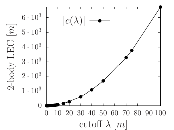
Figure 1: Cutoff $\lambda$ dependence of the coupling strength $c$ of a Gaussian-regulated contact interaction between a pair of particles with an $S$-wave scattering length $a_{0}\approx 10^{5}\,m^{-1}$.

If we use the 2-body potential with the coupling of fig. (1) and in the absence of a 3-body force, the calculated 3-body ground-state energy diverges as the square of the cutoff, i.e., $E_{3}\propto\lambda^{2}$. This is explicitly shown in fig. (5) for the two configurations of fig. (2) – the $\Delta$ and $\Lambda$ configurations – where a parabolic fit to these numerical results finds that

$$E_{3\Lambda}\simeq-0.000118\,\lambda^{2}\quad\text{and}\quad E_{3\Delta}\simeq-0.0596\,\lambda^{2}\,.\qquad$$ (14)

That is, we find a more rapid collapse of the fully resonant $\Delta$ configuration compared with the $\Lambda$ configuration.

These 3-body collapses are avoided by including the 3-body contact terms in Eq. (5). The coupling $d(\lambda)$ is calibrated under the condition that the energy of the 3-body ground state remains constant with the cutoff. By choosing $E_{3\Delta}=E_{3\Lambda}=-0.01~{}m$ for both the delta and lambda configurations, we find numerically the $d_{\Delta}(\lambda)$ and $d_{\Lambda}(\lambda)$ behaviors of fig. (3).

Even though we limit ourselves to the calculation of the ground state of the $\Delta$ and $\Lambda$ trimers, the excited states of these systems do in principle display the Efimov effect Efimov (1970). The discrete scale invariance that characterizes the Efimov effect manifests differently for the $\Delta$ and $\Lambda$ 3-body systems Naidon and Endo (2017): while for the delta configuration, we have the well-known scaling $E^{(n+1)}_{3\Delta}/E^{(n)}_{3\Delta}\simeq(22.7)^{2}$, for the lambda configuration, the scaling is $E^{(n+1)}_{3\Lambda}/E^{(n)}_{3\Lambda}\simeq(1986.1)^{2}$ instead. The superscript $(n)$ indicates the $n$-th excited state of the trimer. We have not checked these two geometric factors that characterize the Efimov spectra specifically in this work. Yet, the $\Delta$ configuration collapses more rapidly than the $\Lambda$, which reflects the smaller discrete scaling factor of the former ($22.7$ for the $\Delta$) compared to the later ($1986.1$ for the $\Lambda$).

lambda($\Lambda$)	delta($\Delta$)

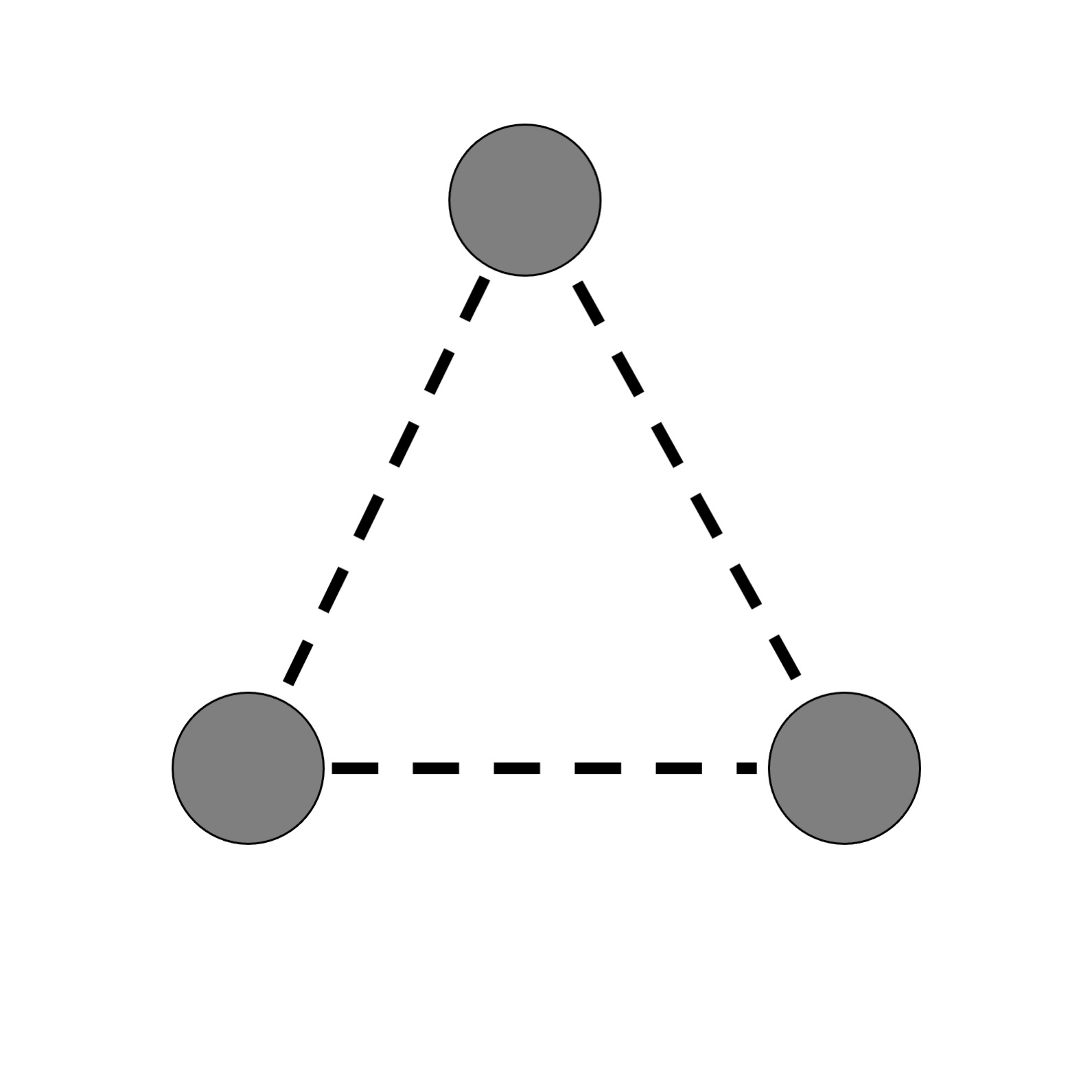
Figure 2: 3-body systems with 2 ($\Lambda$) and 3 ($\Delta$) resonant pairs: the gray circles and dashed lines represent the distinguishable particles and their unitary interactions, respectively.

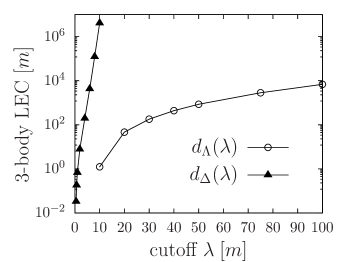
Figure 3: The running of the 3-body coupling strength $d(\lambda)$ which renormalizes the fully resonant (filled triangles) and the 2-pair resonant (empty circles) 3-body systems to a single bound state with $E_{3}=0.01~{}m$.

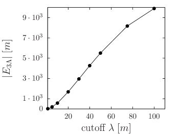
Figure 4: Divergent behavior of ground-state energy $E_{3\Delta}$ of the $\Delta$ 3-body system (three resonant pairs) when we include the 3-body force that renormalized the $\Lambda$ 3-body system (two resonant pairs).

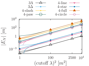
Figure 5: Regulator dependence of the 3- and 4-body ground-state binding energies without any collapse-preventing 3-body interaction. The lines highlight the $\propto\lambda^{2}$ dependence of the binding energies of the states.

III The 4-body sector

III.1 Renormalization

Next, we consider all unitary 4-body systems in which the resonant 2-body interactions form a connected graph. There are six such configurations which we list in fig. (6).

In the absence of 3-body forces, the ground-state energy of each of these 4-body configurations exhibits the quadratic collapse with respect to the regulator $\lambda$ that we encountered in the 3-body case, Eq. (14). The reason is the presence of at least one $\Delta$ or $\Lambda$ subgraph in each of the connected 4-body graphs. These subgraphs will collapse in the absence of 3-body forces as discussed in the previous section.

The inclusion of a 3-body force (see Sec. II) solves the problematic collapse. However, there is an ambiguity regarding which 3-body force to use: as shown in the previous section, the 3-body coupling $d(\lambda$) defined in Eq. (5) has two possible solutions depending on whether the 3-body systems is $\Delta$- or $\Lambda$-shaped. In our calculations, only one choice for the running of $d$ with $\lambda$ was able to properly renormalize the system and generate a finite binding energy. Our numerical results for employing the two runnings in the various graphs (fig. (6)) are summarized graphically in fig. (7). From these results, we infer the following correspondence between a unitary graph and the running of the 3-body force:

• the full, slash, paw and circle graphs require $d_{\Delta}(\lambda)$,

• the line and the star graphs require $d_{\Lambda}(\lambda)$.

This is a rather intuitive result, except for the circle: naively, we would expect that the renormalization of a 4-body system will only require a $\Delta$-type 3-body coupling $d_{\Delta}(\lambda)$ if its unitary graph contains one or more $\Delta$-shaped subgraphs. Conversely, if there are only $\Lambda$-type subgraphs, a $d_{\Lambda}(\lambda)$ coupling should suffice. This is indeed what happens in five of the six configurations where, as we will see, this behavior can be understood in terms of a relatively simple heuristic argument grounded on the Bethe-Peierls boundary conditions for each of these systems. The circle is a remarkable exception: numerically we find that it requires $d_{\Delta}(\lambda)$ – the 3-body coupling that renormalizes the $\Delta$-shaped 3-body system – although it does not contain $\Delta$ subgraphs.

In the upper panel of fig. (7) we show the cutoff dependence of the 4-body binding energy for the configurations that require $d_{\Delta}(\lambda)$. The quantitative ratios we find are:

$$E_{{\rm 4-full}} = 4.4(1)\,E_{3\Delta}\,,$$ (15)

$$E_{{\rm 4-slash}} = 1.8(1)\,E_{3\Delta}\,,$$ (16)

$$E_{{\rm 4-paw}} \approx 1.0\,E_{3\Delta}\,,$$ (17)

$$E_{{\rm 4-circle}} \approx 0.2\,E_{3\Delta}\,,\qquad$$ (18)

where for the full configuration we reproduce the well-known relation between the binding energy of the unitary 3- and 4-boson system. For the circle, the 4-body binding energy is smaller than the 3-body $\Delta$-type configuration. This is not a problem because the circle cannot decay into a 3-body $\Delta$ bound system and a free particle. Notice that the line and star configurations are not shown in the upper panel of fig. (7) simply because when $d_{\Delta}(\lambda)$ is applied to them it happens to be too repulsive to allow for a bound state below the 3-body threshold.

Now, if we use the $d_{\Lambda}(\lambda)$ coupling instead, only the line and star configurations converge, while the full, slash, paw, and circle collapse (see lower panel of fig. (7)). For the line and star configurations, we find

$$E_{{\rm 4-star}} = 11(1)\,E_{3\Lambda}\,,$$ (19)

$$E_{{\rm 4-line}} = 8(1)\,E_{3\Lambda}\,.\qquad$$ (20)

These ratios are not of order one. They are also certainly larger than the respective ratios for the full, slash, paw, and circle.

III.2 Combinatorial approximation to binding

The renormalized binding energy ratios that we have calculated reveal an intriguing pattern: they are proportional to the number of interacting triplets in that system. First, we consider the $\Delta$-like configurations (except the 4-circle, which is the 4-body system that behaves in a more peculiar way). The number of interacting triplets is

$$4\,:\,2\,:\,1\,,$$ (21)

for the full, slash, and paw configurations, respectively. This is to be compared with the ratios of their binding energies:

$$4.4(1)\,:\,1.8(1)\,:\,1\,.$$ (22)

For the $\Lambda$-like configurations (star and line) the number of interacting triplets is

$$3\,:\,2\,,$$ (23)

while the ratios of their binding energies are

$$2.8(6)\,:\,2\,,$$ (24)

and thus in agreement with the ratios of interacting triplets. The uncertainties result from propagating the errors in the binding energies of the different configurations.

Another prediction that can be derived from the combinatorial argument is noteworthy: the binding energy of the $N$-body full configuration. For this prediction, we have to first consider the paw configuration, i.e., a $\Delta$ graph with a fourth particle interacting resonantly with one of the particles forming the $\Delta$. Owing to the resonant nature of this interaction, the naïve expectation is that the binding energy of the odd particle with the $\Delta$ 3-body subsystem will be just below the $\Delta$ plus free particle threshold, which is precisely what is expressed by Eq. (17). In fact, this argument could be extended for an $N$-body system composed of a $\Delta$ followed by a line of $N-3$ particles – the $N$-paw or the $(3,N-3)$-tadpole graph – for which the binding energy will approximately be that of the $\Delta$ 3-body system:

$$E_{N{\rm-paw}}\approx 1.0\,E_{3\Delta}\,.$$ (25)

It is possible that this relation becomes less accurate as the tail of the tadpole, i.e., the chain of particles attached to the $\Delta$ subgraph, becomes longer.

If we return now to the full $N$-body system, the previous assumption together with the combinatorial hypothesis leads to the following ansatz:

$$E_{N{\rm-full}} \approx \begin{pmatrix}N\\ 3\end{pmatrix}\,E_{N{\rm-paw}}\approx\frac{N(N-1)(N-2)}{6}\,E_{3\Delta}$$ (26)

$$\approx \{1,4,10,20,35,56\,\dots\}\,E_{3\Delta}$$

$$\quad\mbox{for $N=3,4,5,6,7,8\,\dots$}\,,$$

where in the second line we specified the values for different numbers of particles. This approximation eventually breaks as $N$ increases. For contact-range forces, in general, we expect that for high enough $N$ the binding energy of these systems will display saturation, that is, a binding energy proportional to the number of particles $N$. As the ground state of the full $N$-body system is as bound as the unitary $N$-boson system , we can compare our results with the ratios obtained for the latter, which have been extensively studied in the literature. If we use the ratios obtained in Ref. von Stecher (2010)

$$E_{N{\rm-full}} = \{1.0,4.7,10.6,18.6,27.9,38.9\,\dots\}\,E_{3\Delta}$$ (27)

$$\quad\mbox{for $N=3,4,5,6,7,8\,\dots$}\,,$$

then we see that even though the combinatorial argument works well for $N\leq 6$ eventually its uncertainties end up increasing with $N$ (about $18,6,7,21,31\%$ for $N=4,5,6,7,8$). If we use instead the more recent calculation of Bazak et al. (2016), the ratios for $N=3,4,5$ will be in better agreement with our approximation

$$E_{N{\rm-full}} = \{1.0,4.2,9.5,16.3\,\dots\}\,E_{3\Delta}$$ (28)

$$\quad\mbox{for $N=3,4,5,6\,\dots$}\,,$$

though we are limited to $N\leq 6$ in this case. Finally, as the number of particles grows, saturation properties emerge (i.e., $E_{N{\rm-full}}$ becomes proportional to $N$, as has been shown in Carlson et al. (2017)) and our combinatorial approximation will cease to be valid.

full	slash
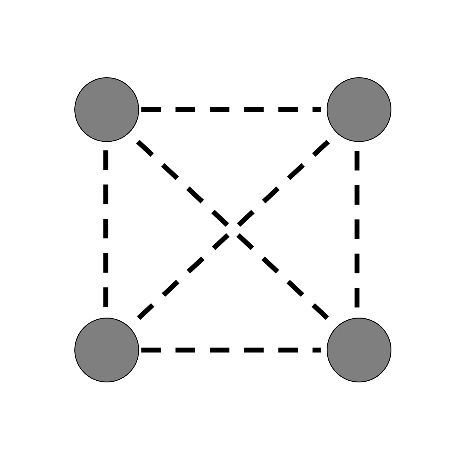
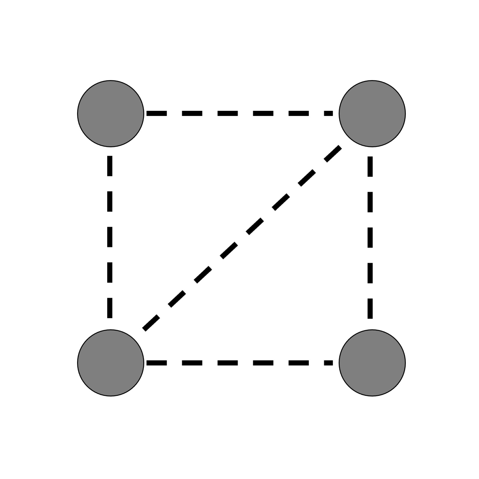
circle	line
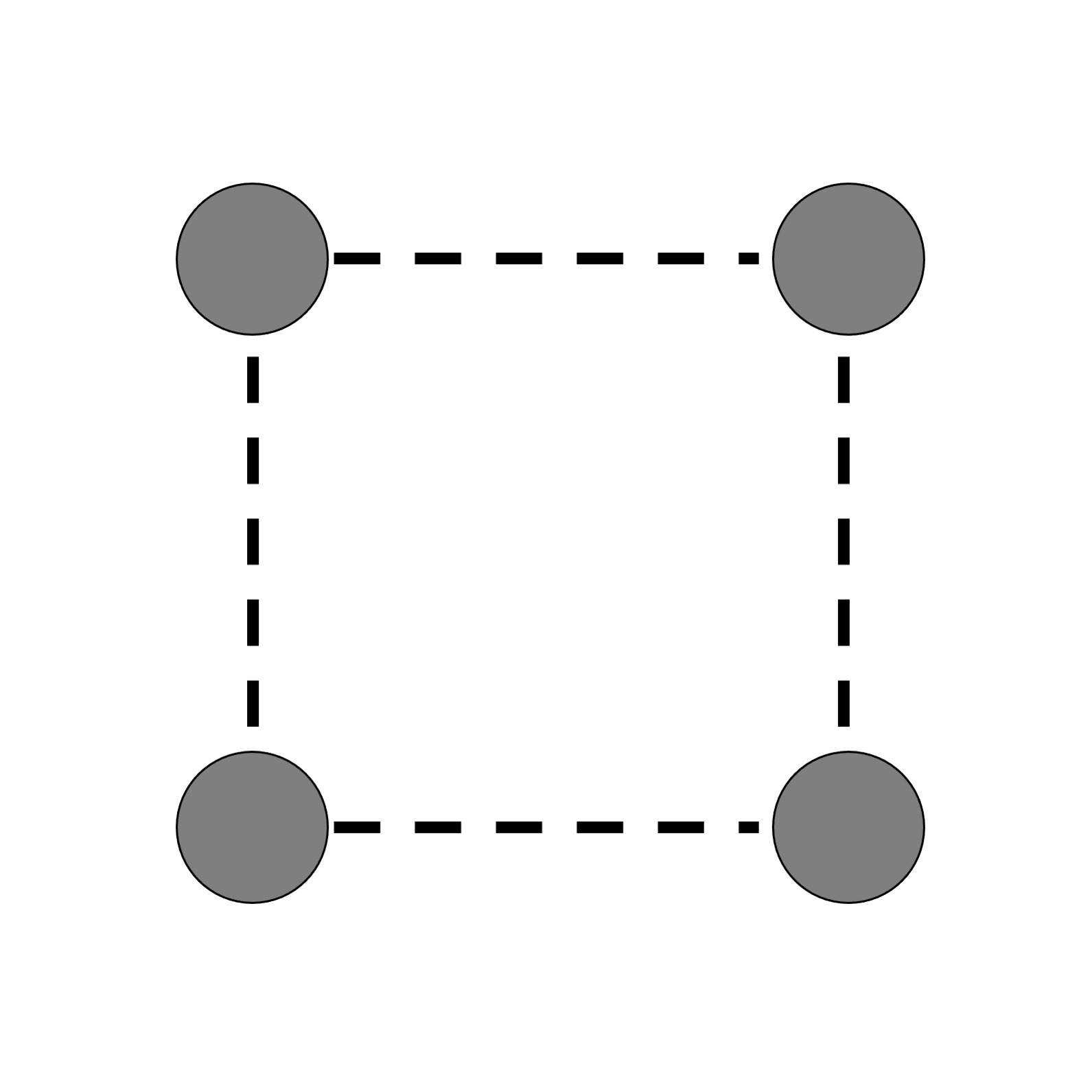
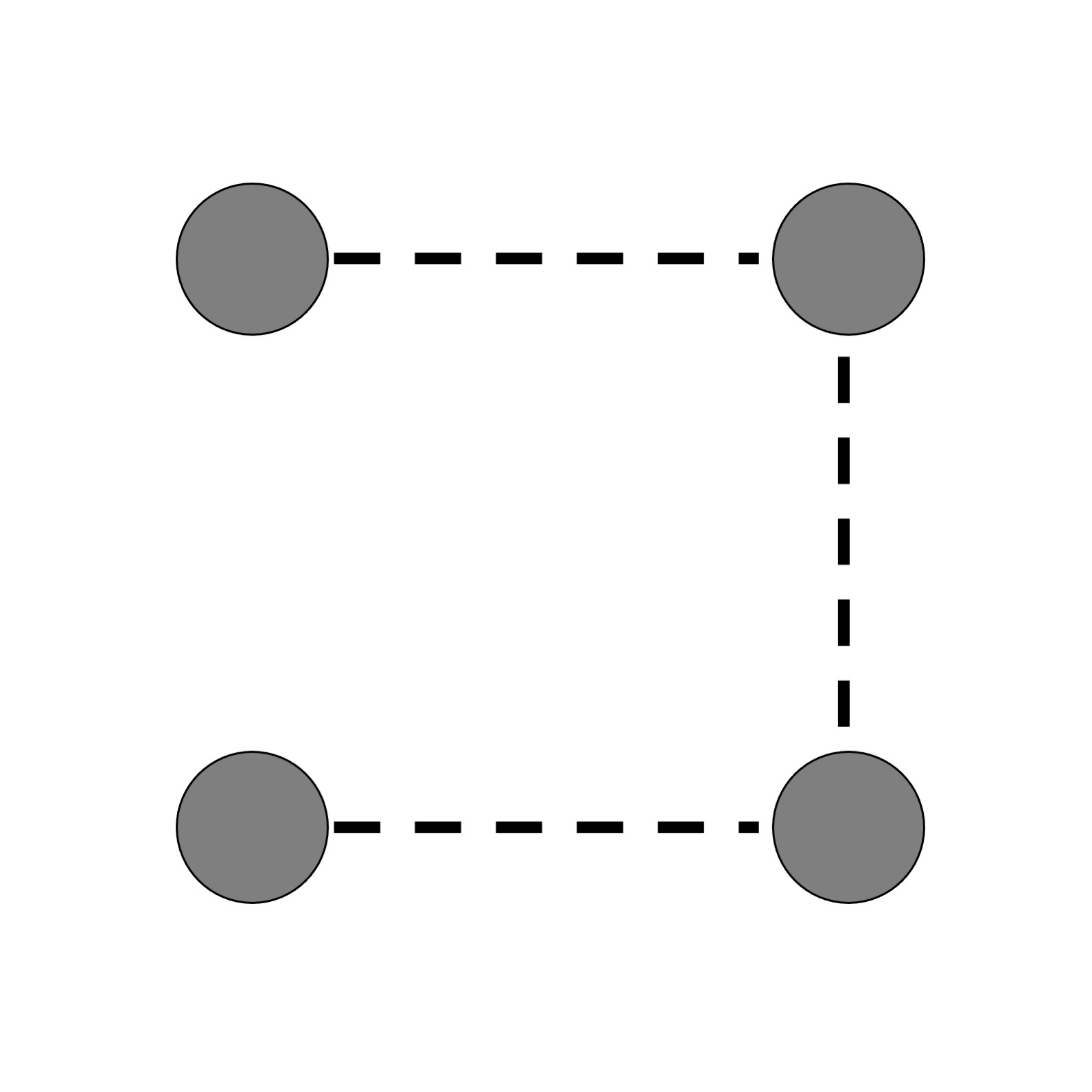
paw	star

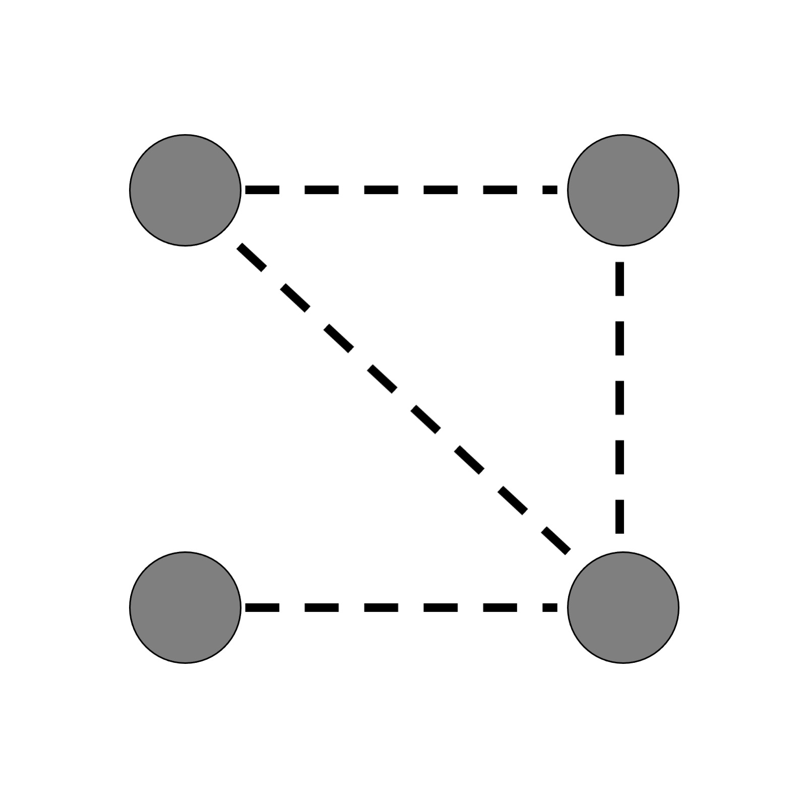
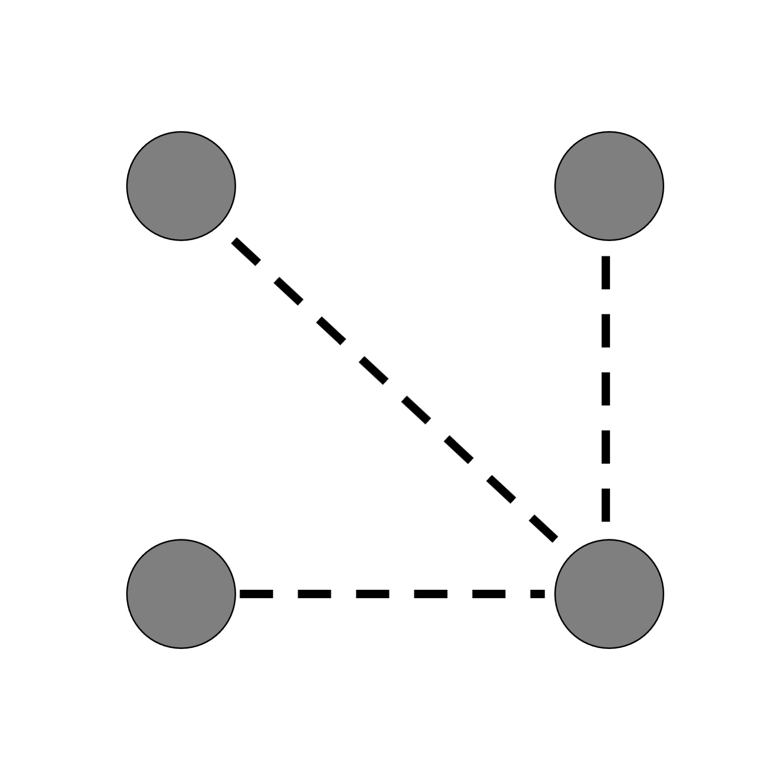
Figure 6: Configurations of 4 distinguishable particles (gray vertices) for which their resonant pair interactions (dashed lines) form a connected graph.

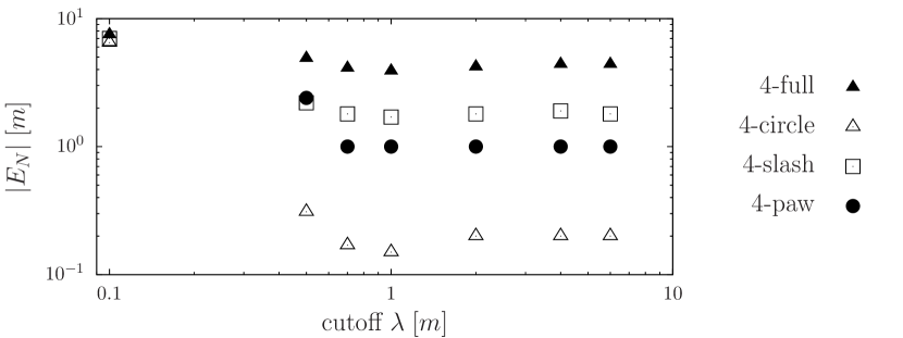
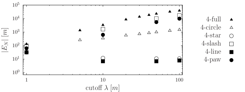
Figure 7: Regulator dependence of the ground-state energy of the six 4-body configurations if the running of the 3-body counter-term is set in the fully-resonant 3-body system (upper panel, $d_{\Delta}$) and in the 2-pair-resonant 3-body system (lower panel, $d_{\Lambda}$).

IV The 5-circle and the unitary loop conjecture

Next, we consider 5-body unitary systems. In this case there are a large number of connected unitary graphs – 21 configurations – and for practical reasons we will focus on a few unitary geometries only.

The specific 5-body configurations we study are the 5-full, 5-circle, and 5-star graphs as shown in fig. (8). The reasons for this selection are

• to verify that the 5-full and 5-star configurations are renormalized by the $d_{\Delta}(\lambda)$ and $d_{\Lambda}(\lambda)$ couplings, respectively, and

• to further confirm the exceptional status of the circle in the 5-body case, i.e., the fact that its proper renormalization requires the $d_{\Delta}(\lambda)$ coupling despite not containing any $\Delta$ subgraph.

The two hypotheses do indeed hold: in the case of the 5-full and 5-circle configurations we numerically find the binding energies to be

$$E_{{\rm 5-full}}\approx 10.8\,E_{3\Delta}\,,$$ (29)

$$E_{{\rm 5-circle}}\approx 0.06\,E_{3\Delta}\,.$$ (30)

We note, again, that the 5-circle cannot decay into other bound states. Hence, there is no problem with its binding energy being smaller than the 3-body $\Delta$ system. For the 5-star we have instead

$$E_{{\rm 5-star}}\approx 30\,E_{3\Lambda}\,,$$ (31)

which follows the trend of binding energies much larger than one, cf., the 4-star and 4-line, Eqs. (19) and (20).

Both findings, those regarding the 4- and 5-circle, suggest the following conjecture: few-body systems whose unitary interactions form a graph containing a closed loop will be renormalized by the 3-body force that renormalizes the 3-body $\Delta$-shaped system (which, incidentally, can also be labeled as the 3-circle). Intuitively, this observations should hold for unitary systems containing 3-, 4-, or 5-circle subgraphs: if the circle component is not renormalized properly, neither will be the system of which it is a part of. However, even though the general idea does not seem implausible, we have not found a rigorous proof yet.

5-full	5-star	5-circle

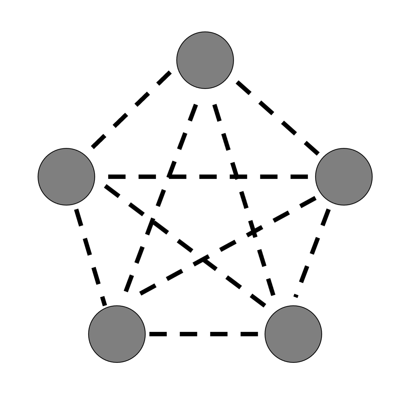
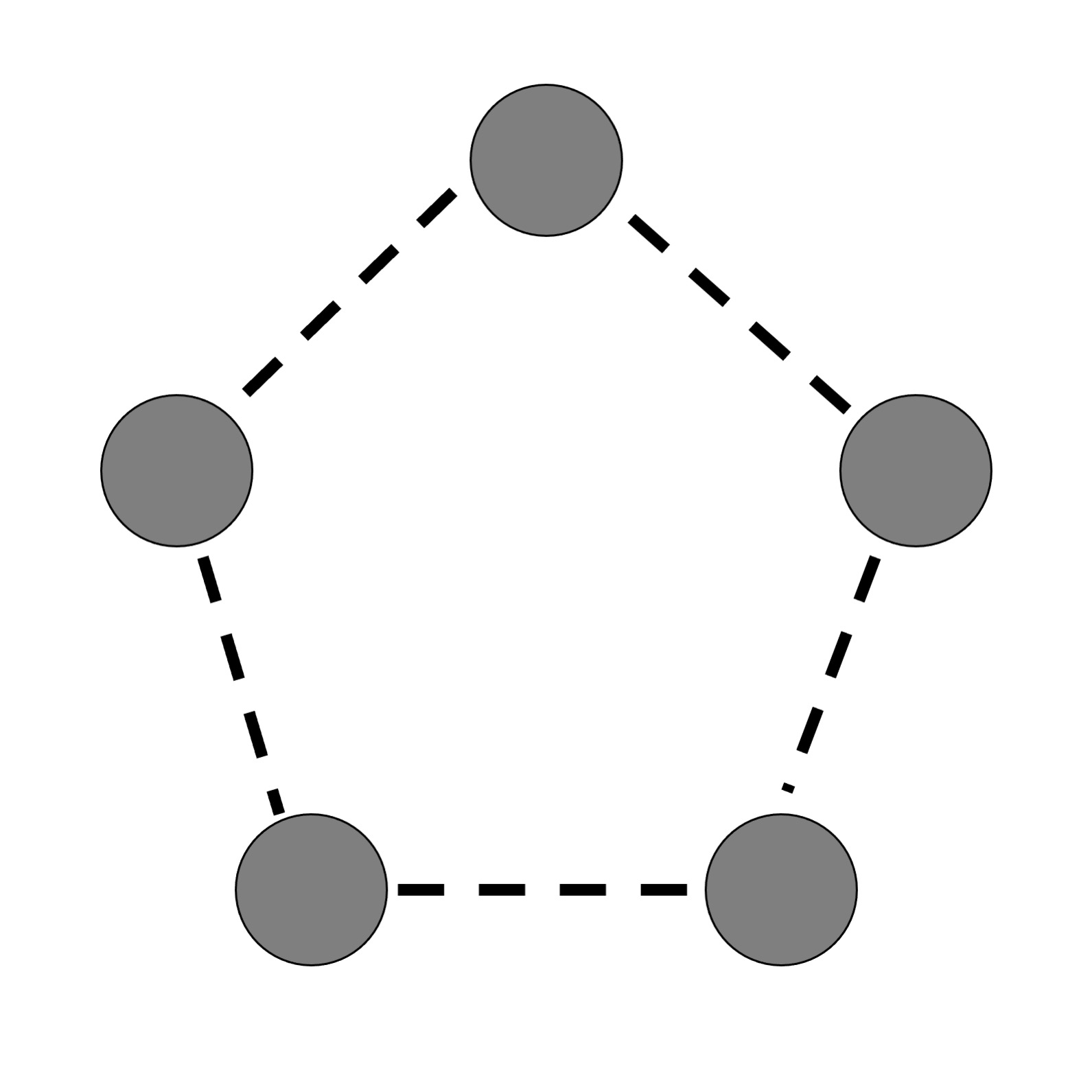
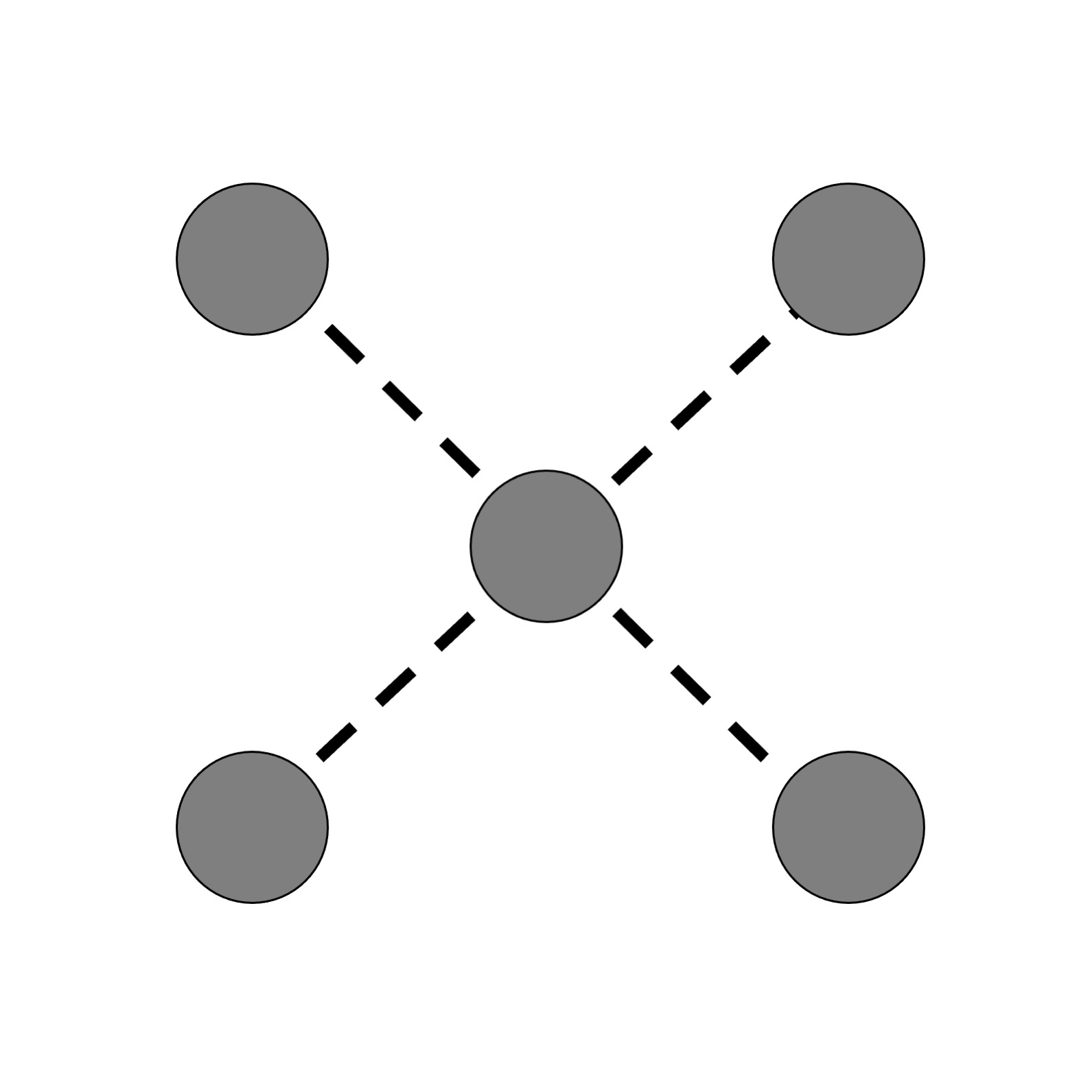
Figure 8: The three connected 5-body shapes considered in this work.

V Explaining the two 4-body renormalization patterns

The renormalization of the 4-body unitary systems falls into two distinct patterns: $\Delta$- and $\Lambda$-like. Here we present a heuristic argument of why this is the case. We stress that this is not a rigorous derivation of those renormalization patterns, and yet, the explanation we provide, though incomplete, helps to clarify in which cases we should expect each type of 3-body force.

For understanding the patterns we will consider a zero-range 2-body resonant interaction. That is, we will be considering the $\lambda\to\infty$ (or zero-range) limit, in which a 2-body resonant interaction is reduced to a boundary condition of the wave function at the origin, that is:

$$\frac{d}{dr_{lk}}\left[r_{lk}\Psi_{N}\right]\Big{|}_{r_{lk}=0}=0\,,$$ (32)

for each $l$, $k$ particle pair for which the interaction is resonant ($\vec{r}_{l}$ and $\vec{r}_{k}$ are single-particle coordinates and $\vec{r}_{lk}=\vec{r}_{l}-\vec{r}_{k}$). The Faddeev-component expansion of the $N$-body wave function

$$\Psi_{N}=\sum_{ij}\psi_{ij}(\vec{r}_{ij},\dots)\,,$$ (33)

yields

$$\frac{d}{dr_{lk}}\left[r_{lk}\psi_{lk}\right]+\sum_{ij\neq lk}\psi_{ij}(\vec{r}_{ij},\dots)\Big{|}_{r_{lk}=0}=0\,.$$ (34)

In general, this set of equations will simplify owing to symmetries that reduce the number of independent Faddeev components. For instance, in the $N$-boson system or in the full $N$-body unitary system, all the Faddeev components will be identical, i.e., $\psi_{ij}=\psi$; in the first case this happens because of Bose-Einstein symmetry and in the second because of symmetry under the permutation group.

In the 3-body system it is well-known how to derive the Efimov scaling from the boundary condition in Eq. (32). Though we will not present here the full derivation (which can be found in Fedorov and Jensen (1993)), we will try to understand the general patterns leading to the different types of discrete scaling in the 3-body system (i.e., the standard $22.7$ discrete scaling for the 3-boson system and the $1986.1$ scaling for the heteronuclear case with equal masses). In the $\Delta$ case, if we particularize the boundary condition for $lk=12$ as a reference, we get

$$\frac{d}{dr_{12}}\left[r_{12}\psi(\vec{r}_{12},\vec{\rho}_{3})\right]\Big{|}_{r_{12}=0}$$

$$\quad+\psi(\vec{r}_{23},\vec{\rho}_{1})\Big{|}_{r_{12}=0}+\psi(\vec{r}_{31},\vec{\rho}_{2})\Big{|}_{r_{12}=0}=0\,,$$ (35)

where we have already taken into account that the three Faddeev components of the wave function are formally identical, and $\vec{\rho}_{k}=\vec{r}_{k}-(\vec{r}_{i}+\vec{r}_{j})/2$ (plus the condition $i\neq j\neq k$) being one of the Jacobi coordinates. After suitable manipulations, the previous boundary condition will lead to the standard Efimov effect with a discrete scaling of $22.7$. In the $\Lambda$ system, we obtain instead

$$\frac{d}{dr_{12}}\left[r_{12}\psi(\vec{r}_{12},\vec{\rho}_{3})\right]\Big{|}_{r_{12}=0}+\psi(\vec{r}_{31},\vec{\rho}_{2})\Big{|}_{r_{12}=0}=0\,,$$

(36)

which translates into a discrete scaling of $1986.1$. The specific steps leading from Eqs. (35) and (36) to the respective discrete scale symmetry of these two systems are well-known (see, e.g., Ref. Naidon and Endo (2017)).

This argument can be easily extended to the 4-body system. We will illustrate the idea with the 4-full system for which

$$\frac{d}{dr_{12}}\left[r_{12}\psi(\vec{r}_{12},\dots)\right]\Big{|}_{r_{12}=0}$$

$$\quad+\sum_{ij\neq 12}\psi(\vec{r}_{ij},\dots)\Big{|}_{r_{12}=0}=0\,.$$ (37)

Superficially, this boundary condition does not seem to be equivalent to the corresponding ones in the 3-body case. A more careful inspection reveals that this is not the case. Indeed, the six Faddeev components can be subdivided further depending on the different choices of Jacobi coordinates (i.e., into Faddeev-Yakubovsky components). To provide a concrete example, we might expand the $ij=12$, $23$, and $13$ components as

$$\psi(\vec{r}_{12},\dots) = \psi_{K}(\vec{r}_{12},\vec{\rho}_{3},\vec{\sigma}_{4})+\psi_{K}(\vec{r}_{12},\vec{\rho}_{4},\vec{\sigma}_{3})$$ (38)

$$+ \psi_{H}(\vec{r}_{12},\vec{h}_{12-34},\vec{r}_{34})\,,$$

$$\psi(\vec{r}_{23},\dots) = \psi_{K}(\vec{r}_{23},\vec{\rho}_{1},\vec{\sigma}_{4})+\psi_{K}(\vec{r}_{23},\vec{\rho}_{4},\vec{\sigma}_{1})$$ (39)

$$+ \psi_{H}(\vec{r}_{23},\vec{h}_{23-14},\vec{r}_{14})\,,$$

$$\psi(\vec{r}_{31},\dots) = \psi_{K}(\vec{r}_{31},\vec{\rho}_{2},\vec{\sigma}_{4})+\psi_{K}(\vec{r}_{31},\vec{\rho}_{4},\vec{\sigma}_{2})$$ (40)

$$+ \psi_{H}(\vec{r}_{31},\vec{h}_{31-24},\vec{r}_{24})\,,$$

where we use the customary subscripts $K$ and $H$ to indicate the K- and H-components. For the $K$ set of Jacobi coordinates, we have $\vec{\rho}_{k(ij)}=\vec{r}_{k}-(\vec{r}_{i}+\vec{r}_{j})/2$ (though usually the $ij$ subscript will be dropped, as it always corresponds to that of the first coordinate $\vec{r}_{ij}$) and $\vec{\sigma}_{l}=\vec{r}_{l}-(\vec{r}_{i}+\vec{r}_{j}+\vec{r}_{k})/3$ with $i\neq j\neq k\neq l$, while for the $H$ set we only have one new coordinate: $\vec{h}_{ij-kl}=(\vec{r}_{i}+\vec{r}_{j})/2-(\vec{r}_{l}+\vec{r}_{l})/2$.

The bottom line is that the original $12$ boundary condition can be subdivided into two different types of boundary conditions. One type involves the K-components only: for instance, if we separate the Faddeev-Yakubovsky components that contain the $\sigma_{4}$ Jacobi coordinate, we get

$$\frac{d}{dr_{12}}\left[r_{12}\,\psi_{K}(\vec{r}_{12},\vec{\rho}_{3},\vec{\sigma}_{4})\right]\Big{|}_{r_{12}=0}$$

$$\quad+\psi_{K}(\vec{r}_{23},\vec{\rho}_{1},\vec{\sigma}_{4})\Big{|}_{r_{12}=0}+\psi_{K}(\vec{r}_{31},\vec{\rho}_{2},\vec{\sigma}_{4})\Big{|}_{r_{12}=0}=0\,.$$

(41)

If we ignore the $\vec{\sigma}_{4}$ coordinate (which does not play a direct role in the boundary condition), one realizes that this type of boundary condition is equivalent to the one in the $\Delta$ system (Eq.  (35)). We thus expect it to generate the same type of Efimov scaling, namely $22.7$, which also implies that the 3-body force that renormalizes the $\Delta$ would renormalize the complete system. We also notice that any few-body configuration containing a $\Delta$ subsystem should contain a version of the boundary condition above, implying the $22.7$ discrete scaling factor and its eventual renormalizability by means of the $d_{\Delta}(\lambda)$ 3-body force. In addition, there will be a different boundary condition for the H-components, which we do not write down here: this second boundary condition is not trivial to interpret, but we suspect that it is related to the existence of two different universal solutions for the 4-boson system Hammer and Platter (2007).

The extension to the other 4-body systems that contain at least a $\Delta$ subsystem (i.e., a closed loop of three resonant interactions) is laborious (as not all the Faddeev components are identical) but straightforward. It eventually leads to the boundary condition of Eq. (41)  from which we expect to obtain the same discrete scaling as the $\Delta$ (i.e., $22.7$). It is thus no surprise that these systems will be renormalized by the $\Delta$ 3-body force.

The extension to the 4-star is trivial, the most important difference being the reduced number of Faddeev components (4 instead of 6). If we assume that only the $1j$ interactions with $j=2,3,4$ are resonant, we have the boundary condition

$$\frac{d}{dr_{12}}\left[r_{12}\psi(\vec{r}_{12},\dots)\right]\Big{|}_{r_{12}=0}$$

$$\quad+\sum_{j\neq 1}\psi(\vec{r}_{1j},\dots)\Big{|}_{r_{12}=0}=0\,.$$ (42)

After expanding the Faddeev components into Faddeev-Yakubovsky ones, we will end up with the following boundary condition for the K-components

$$\frac{d}{dr_{12}}\left[r_{12}\,\psi_{K}(\vec{r}_{12},\vec{\rho}_{3},\vec{\sigma}_{4})\right]\Big{|}_{r_{12}=0}$$

$$\quad+\psi_{K}(\vec{r}_{31},\vec{\rho}_{2},\vec{\sigma}_{4})\Big{|}_{r_{12}=0}=0\,.$$ (43)

This condition is formally identical to the one in the $\Lambda$-shaped 3-body system except for the additional coordinate $\vec{\sigma}_{4}$ (which, again, does not play a direct role in the boundary condition). Thus the conclusion is that its discrete scaling behavior should be identical to that of the $\Lambda$-shaped 3-body system from which it follows that it is also renormalized by the $\Lambda$ 3-body force, $d_{\Lambda}(\lambda)$. Again, though laborious, this argument can be extended to any $N$-body system for which the unitary graph is a tree.

Now the problem lies with $N$-body systems that contain a unitary loop with more than three lines, e.g., the 4-circle. The boundary condition for the 4-circle reads

$$\frac{d}{dr_{12}}\left[r_{12}\,\psi(\vec{r}_{12},\dots)\right]\Big{|}_{r_{12}=0}$$

$$\quad{+\psi(\vec{r}_{23},\dots)+\psi(\vec{r}_{34},\dots)+\psi(\vec{r}_{41},\dots)}\,\Big{|}_{r_{12}=0}$$

$$\quad=0\,,$$ (44)

which, if expanded and matched in terms of K-type Jacobi coordinates and Faddeev-Yakubovsky components, will result in a variation of the boundary condition of the 4-star, i.e., in Eq. (43). However, our concrete calculations with the 4-circle show otherwise. This indicates that our argument is incomplete for the 4-circle, which points toward some overlooked factors in the previous arguments. We conjecture that the missing factor is most probably a non-optimal choice of Jacobi coordinates and Faddeev-Yakubovsky components, which ignores the cyclical permutation symmetry of this system. Basically, what we have been able to show is that the Bethe-Peierls boundary condition for the 4-circle contains a boundary subcondition similar to that of the $\Lambda$-shaped 3-body system, Eq. (36). Yet, this does not preclude the possibility that a different choice of coordinates and components might uncover the presence of the more stringent boundary condition of the $\Delta$-shaped 3-body system. Indeed we know this to be the case owing to our numerical finding that the 4-circle requires the $d_{\Delta}(\lambda)$ 3-body force for its proper renormalization. This situation also repeats itself for the 5-circle, which leads us to the conjecture that all unitary clusters containing a closed unitary interaction loop should have the same scaling as in the standard Efimov effect, i.e., $22.7$.

Nonetheless, some unclear signals come from previous works in this sense. In ref. Naidon (2018), the 4-circle has been studied using the same renormalization scheme as for the lambda system. The energy of the 4-circle was found to be unnaturally large, $\sim$400 E₃, and thereby indicative for a collapsing system and an associated new scale. However, in the mass-imbalanced 4-circle the Efimovian excitation structure was found compatible with the mass-imbalanced lambda-system discrete scaling, in contradiction with our conjecture. This may be explained by a transition of the Efimovian structure from Delta to Lambda-like induced by an increasing mass ratio. This explanation is consistent with the more recent ref. Frederico et al. (2019) where it was found that the geometric scaling of the 4-body two-species system with a mass imbalance is smaller than the corresponding scaling of its 3-body counterpart. However, the arguments in Frederico et al. (2019) depend explicitly on the existence of a large difference in masses between the two species and are thus not directly applicable to our 4-circle configuration. We conclude that, despite there are no yet clear contradictions in the studies published up to now, more attention to the spectral structure of the 4-circle is needed.

VI Conclusions

We have analyzed partially unitary few-body systems in which all particles have the same mass but not all interparticle interactions are resonant, only a subset of them. Each of these few-body systems can be characterized by a unitary graph, whose vertices and lines represent particles and resonant interactions, respectively. The resonant interactions can be modeled, without loss of generality, by zero-range potentials, which are singular and require regularization and renormalization. Here, we analyzed the renormalization of the ground states of systems with $N=3$ and $4$ particles (plus a few illustrative $N=5$ configurations).

From a series of numerical calculations and qualitative arguments, we conjecture a relation between the geometry of the unitary graph representing the partially unitary system and its renormalization. Partially unitary few-body systems do display Thomas collapse, i.e., the binding energies of these systems diverge as the range of their interactions approach zero. As in the 3-body case, this collapse is avoided by the inclusion of a zero-range, repulsive 3-body force which stabilizes the binding energy of the ground state. The type of 3-body force renormalizing a partially unitary 4-body system (of which there are six, see fig. (6)) depends on the properties of the unitary graph of the latter:

• unitary tree-like graphs require the 3-body force that renormalizes the 3-body system with two resonant pairs (which we have called the $\Lambda$ system),

• unitary graphs containing closed loops are renormalized instead by the 3-body force of the 3-body system with three resonant pairs (which we have called the $\Delta$ system).

We have deduced (and verified) this renormalization pattern numerically for each of the 4-body unitary graphs. We conjecture that this pattern extends to partially unitary systems with $N>4$, though we have only verified this generalization numerically for three selected $N=5$ systems.

Furthermore, we have proposed a heuristic argument that exploits the representation of a resonant pair in terms of a Bethe-Peierls boundary condition to show that the different 4-body unitary graphs are indeed expected to be renormalized by the 3-body force of the $\Lambda$- or $\Delta$-shaped systems. More specifically, what we have shown is that the resonant 2-body interaction imposes a constraint on the 4-body wave function that is identical to the analogous constraint for the 3-body system (modulo the presence of an additional coordinate for the extra particle). Incidentally, this is the same constraint that generates the characteristic discrete scale invariance of $22.7$ and $1986.1$ for the $\Delta$- and $\Lambda$-shaped 3-body systems. Hence, we conjecture that the discrete scaling properties of a particular unitary graph will follow one of these two patterns (depending on whether they are renormalized by the 3-body force of the $\Delta$- or $\Lambda$-shaped systems). However, the argument fails for the particular case of cyclic graphs – the $N$-circles in the naming convention we follow – which indicates that our explanation of this behavior is incomplete, representing an intriguing open problem which is left to future work.

References

- Braaten and Hammer (2006) E. Braaten and H. W. Hammer, Phys. Rept. 428, 259 (2006), eprint cond-mat/0410417.
- Efimov (1970) V. Efimov, Phys. Lett. 33B, 563 (1970).
- Kraemer et al. (2006) T. Kraemer, M. Mark, P. Waldburger, J. G. Danzl, C. Chin, B. Engeser, A. D. Lange, K. Pilch, A. Jaakkola, H.-C. Nägerl, et al., Nature 440, 315 (2006).
- Carlson et al. (2017) J. Carlson, S. Gandolfi, U. van Kolck, and S. Vitiello, Phys. Rev. Lett. 119, 223002 (2017), eprint 1707.08546.
- Helfrich et al. (2010) K. Helfrich, H. W. Hammer, and D. S. Petrov, Phys. Rev. A81, 042715 (2010), eprint 1001.4371.
- Wang et al. (2012) Y. Wang, W. B. Laing, J. von Stecher, and B. D. Esry, Phys. Rev. Lett. 108, 073201 (2012), URL https://link.aps.org/doi/10.1103/PhysRevLett.108.073201.
- Blume and Yan (2014) D. Blume and Y. Yan, Phys. Rev. Lett. 113, 213201 (2014), URL https://link.aps.org/doi/10.1103/PhysRevLett.113.213201.
- Helfrich and Hammer (2011) K. Helfrich and H. W. Hammer, J. Phys. B44, 215301 (2011), eprint 1107.0869.
- Bazak et al. (2019) B. Bazak, J. Kirscher, S. König, M. Pavón Valderrama, N. Barnea, and U. van Kolck, Phys. Rev. Lett. 122, 143001 (2019), eprint 1812.00387.
- Contessi et al. (2021) L. Contessi, J. Kirscher, and M. P. Valderrama, Phys. Lett. A 408, 127479 (2021), eprint 2103.14711.
- Kartavtsev and Malykh (2007) O. I. Kartavtsev and A. V. Malykh, Journal of Physics B: Atomic, Molecular and Optical Physics 40, 1429 (2007), URL https://dx.doi.org/10.1088/0953-4075/40/7/011.
- Petrov et al. (2004) D. S. Petrov, C. Salomon, and G. V. Shlyapnikov, Phys. Rev. Lett. 93, 090404 (2004), URL https://link.aps.org/doi/10.1103/PhysRevLett.93.090404.
- Naidon and Endo (2017) P. Naidon and S. Endo, Rept. Prog. Phys. 80, 056001 (2017), eprint 1610.09805.
- van Kolck (1999) U. van Kolck, Nucl. Phys. A 645, 273 (1999), eprint nucl-th/9808007.
- Bedaque et al. (1999) P. F. Bedaque, H. W. Hammer, and U. van Kolck, Phys. Rev. Lett. 82, 463 (1999), eprint nucl-th/9809025.
- Bedaque et al. (2000) P. F. Bedaque, H. W. Hammer, and U. van Kolck, Nucl. Phys. A676, 357 (2000), eprint nucl-th/9906032.
- Brandstädt et al. (1999) A. Brandstädt, V. B. Le, and J. P. Spinrad, Graph Classes: A Survey (Society for Industrial and Applied Mathematics, 1999), eprint https://epubs.siam.org/doi/pdf/10.1137/1.9780898719796, URL https://epubs.siam.org/doi/abs/10.1137/1.9780898719796.
- Suzuki and Varga (1998) Y. Suzuki and K. Varga, Stochastic variational approach to quantum-mechanical few-body problems, Lecture Notes in Physics Monographs (Springer, Berlin, 1998), URL https://cds.cern.ch/record/1631377.
- Hofmann (1986) H. Hofmann, in Proceedings of Models and Methods in Few-Body Physics, Lisboa, Portugal, edited by L. Ferreira, A. Fonseca, and L. Streit (1986), p. 243.
- König et al. (2017) S. König, H. W. Grießhammer, H. W. Hammer, and U. van Kolck, Phys. Rev. Lett. 118, 202501 (2017), eprint 1607.04623.
- von Stecher (2010) J. von Stecher, J. Phys. B 43, 101002 (2010), eprint 0909.4056.
- Bazak et al. (2016) B. Bazak, M. Eliyahu, and U. van Kolck, Phys. Rev. A 94, 052502 (2016), eprint 1607.01509.
- Sloane and Inc. (2020) N. J. A. Sloane and T. O. F. Inc., The on-line encyclopedia of integer sequences (2020), URL http://oeis.org/?language=english.
- Stein and Stein (1963) M. L. Stein and P. R. Stein (1963), URL https://www.osti.gov/biblio/4180737.
- Fedorov and Jensen (1993) D. V. Fedorov and A. S. Jensen, Phys. Rev. Lett. 71, 4103 (1993), URL https://link.aps.org/doi/10.1103/PhysRevLett.71.4103.
- Hammer and Platter (2007) H. W. Hammer and L. Platter, Eur. Phys. J. A 32, 113 (2007), eprint nucl-th/0610105.
- Naidon (2018) P. Naidon, Few Body Syst. 59, 64 (2018).
- Frederico et al. (2019) T. Frederico, W. Paula, A. Delfino, M. T. Yamashita, and L. Tomio, Few Body Syst. 60, 46 (2019).