Choosing Public Datasets for Private Machine Learning via Gradient Subspace Distance

Abstract

Differentially private stochastic gradient descent privatizes model training by injecting noise into each iteration, where the noise magnitude increases with the number of model parameters. Recent works suggest that we can reduce the noise by leveraging public data for private machine learning, by projecting gradients onto a subspace prescribed by the public data. However, given a choice of public datasets, it is not a priori clear which one may be most appropriate for the private task. We give an algorithm for selecting a public dataset by measuring a low-dimensional subspace distance between gradients of the public and private examples. We provide theoretical analysis demonstrating that the excess risk scales with this subspace distance. This distance is easy to compute and robust to modifications in the setting. Empirical evaluation shows that trained model accuracy is monotone in this distance.

1 Introduction

Recent work has shown that machine learning (ML) models tend to memorize components of their training data [model-memorize-data], and in fact attackers can often recover training samples from published models through carefully designed attacks [extract-gpt2, membership-infer]. This is a critical privacy issue when models are trained on private data. A popular approach to address this issue is to adopt Differential Privacy (DP) [dwork-dp] as a rigorous privacy criterion that provably limits the amount of information attackers can infer about any single training point. Differentially private stochastic gradient descent (DPSGD) [DP-SGD, dpsgd2, dpsgd3] is one of the most commonly used methods to train a ML model (differentially) privately. It makes two main modifications to vanilla SGD: 1) clipping per-sample gradients to ensure a bound on their $\ell_{2}$ norms; 2) adding Gaussian noise to the gradient.

One downside of adopting DP in ML is that we need to sacrifice utility of the trained model to guarantee privacy. Specifically, DPSGD noises the gradient at each step, with noise drawn from a spherical Gaussian distribution, $\mathcal{N}\left(\mathbf{0},\sigma^{2}\mathbb{I}_{p\times p}\right)$, where $p$ is the model dimension (i.e., the number of model parameters) and the variance $\sigma^{2}$ scales the noise. In order to bound the privacy leakage, the magnitude of noise introduced in each step must scale with the square root of the number of parameters $p$. Consequently, for many large models, the noise introduced may overwhelm the signal contributed by the original gradients, significantly diminishing the utility.

Several works have proposed methods to improve the utility of private machine learning [bypass, aws, cvpr, donot, KairouzRRT21]. One fruitful direction uses public data, i.e., data that is not subject to any privacy constraint. There are primarily two types of approaches that incorporate public data in private training. The first involves transfer learning, where we pretrain the model on a public dataset and then (privately) finetune the model on a sensitive dataset for our target task [cvpr, DP-SGD, YuNBGIKKLMWYZ22, LiTLH22]. Another approach is based on pre-conditioning, which exploits the empirical observation that during training, the stochastic gradients (approximately) stay in a lower-dimensional subspace of the $p$-dimensional gradient space. Consequently, some works find this subspace using the public data, and then project the sensitive gradients to this (public) subspace before privatization [bypass, aws, donot, KairouzRRT21]. This reduces the magnitude of the introduced noise and generally improves utility over DPSGD without supplementary data.

However, this raises a natural question: which public dataset should one select for a particular private task? It may be ideal if a fraction of the private dataset is public, as using it would incur minimal penalty due to distribution shift. But otherwise, it is unclear when one should prefer one public dataset over another. Our main contribution is an algorithm that quantifies a public dataset’s fitness for use in private ML.

Table 1: GEP evaluation AUC and corresponding distance in descending order. We use the same model setting for private training and distance computation. ”-” means DP-SGD training without using any public data.

. AUC Private Dataset Public Dataset Distance 69.02% ChestX-ray14 ChestX-ray14 0.15 66.62% KagChest 0.36 64.90% - - 48.80% CIFAR-100 0.55

We demonstrate its efficacy in both transfer learning and pre-conditioning settings. To summarize our contributions:

1. We introduce Gradient Subspace Distance (GSD), an algorithm to quantify the difference between private and public datasets. GSD is an easily computable quantity that measures the distance between two datasets.

2. We find GSD is useful for selecting public datasets in both pre-conditioning and transfer learning settings. As a representative example, Table 1 shows the utility of a privately trained model using a public dataset increases monotonously as GSD decreases. Our theoretical analysis demonstrates that the excess risk of Gradient Embedding Perturbation (GEP) (a private training algorithm that leverages public data for gradient pre-conditioning) scales with the GSD.

3. We show that GSD is transferable. The ordering of GSD for several choices of public dataset remains fixed across architectures, both simple (e.g., 2-layer CNN) and complex. Using these simple architectures as a proxy, we can efficiently compute GSDs which are still useful for privately training large models.

2 Related Work

Transfer Learning.

In the differentially private setting, it is now common to pre-train a model on public data, and then privately fine-tune on private data. This can result in comparable utility as in the non-private setting, evidenced for both language models [donot, YuNBGIKKLMWYZ22, LiTLH22] and vision tasks [cvpr, DeBHSB22, MehtaTKC22]. In many cases, due to computational requirements, it may be challenging to pre-train a large model on a public dataset. Instead, many practitioners will turn to pre-trained weights, which obviate the computational burden, but give less flexibility to choose an appropriate training dataset. As a result, we use second-phase pre-training, in which we perform a second phase of pre-training with a modestly-sized public dataset. This has been proven to be useful in non-private setting [dontstop].

Pre-conditioning.

Empirical evidence and theoretical analysis indicate that while training deep learning models, gradients tend to live in a lower-dimensional subspace [subspace1, subspace2, subspace3, aws, precondtheo]. This has led to methods for private ML which project the sensitive gradients onto a subspace estimated from the public gradients. By using a small amount of i.i.d. public data, [bypass] demonstrate that this approach can improve the accuracy of differentially private stochastic gradient descent in high-privacy regimes and achieve a dimension-independent error rate. Similarly, [donot] proposed GEP, a method that utilizes public data to identify the most useful information carried by gradients, and then splits and clips them separately.

Domain Adaptation.

We aim to quantify the similarity between private and public datasets. One related area of research is distribution shift, or domain adaptation [distshiftsurvey, distshiftsurvey2, distshiftsurvey3, distshiftsurvey4, Ben-DavidBCKPV10, Ben-DavidBCP06, tent]. At a high level, research in this area examines the problem of when the distributions of test and training data differ, which aligns with our goals. However, most work in this area focuses on reducing the gap between in- and out-of-distribution test errors, where target data is used repeatedly for accuracy improvement. Most of the work along this line assumes that the target data is also public or doesn’t consider privacy, and is thus inappropriate for the private learning setting. To the best of our knowledge, the only work with a similar focus to us is Task2Vec [task2vec], which uses the Fisher information matrix to represent a dataset as a vector, allowing for the measurement of a distance between two datasets. However, it is not suitable for private learning tasks as our empirical evaluation shows that Task2Vec fails to accurately rank the utility of public datasets.

3 Preliminaries

Notation.

We use $p$ to denote the model dimension, i.e., the number of parameters in the model. $k$ is a parameter we will use to denote the dimension of the lower-dimensional space we choose. $m$ refers to the number of examples in a batch. We use superscripts and subscripts interchangeably to denote private or public data, like $x_{priv}$, $V^{pub}$.

Definition 1 (Differential Privacy [dwork-dp]).

A randomized algorithm $\mathcal{A}$ is $(\varepsilon,\delta)$-differential private if for any pair of datasets D, D’ that differ in exactly one data point and for all subsets E of outputs, we have:

$$\Pr[\mathcal{A}(D)\in E]\leq e^{\varepsilon}\Pr[\mathcal{A}(D^{\prime})\in E]+\delta.$$

Definition 2 (Principal Angles [principleangles]).

Let $V_{1}$ and $V_{2}$ be two orthonormal matrices of $\mathbb{R}^{p\times k}$. The principal angles $0\leq\theta_{1}\leq\cdot\cdot\cdot\leq\theta_{k}\leq\pi/2$ between two subspaces span($V_{1}$) and span($V_{2}$), are defined recursively by

$$\cos\theta_{k}=\max\limits_{\mathbf{u_{k}}\in span(V_{1})}\max\limits_{\mathbf{v_{k}}\in span(V_{2})}\mathbf{u_{k}^{\prime}v_{k}},\ \ \textit{subject to}$$

$$\mathbf{u_{k}^{\prime}u_{k}}=1,\mathbf{v_{k}^{\prime}v_{k}}=1,\mathbf{u_{k}^{\prime}u_{i}}=0,\mathbf{v_{k}^{\prime}v_{i}}=0,i=1,...,k-1$$

That is, the first principal angle $\theta_{1}$ is the smallest angle between all pairs of unit vectors over two subspaces, the second $\theta_{2}$ is the second smallest angle, and the rest are similarly defined.

Definition 3 (Projection Metric [projectionmetric, projectionmetric2]).

The projection metric between two $k$-dimensional subspaces $V_{1}$, $V_{2}$ is defined as:

$$d\left(V_{1},V_{2}\right)=\left(\sum_{i=1}^{k}\sin^{2}\theta_{i}\right)^{1/2}=\left(k-\sum_{i=1}^{k}\cos^{2}\theta_{i}\right)^{1/2}$$

where the $\theta_{i}$’s are the principal angles between $V_{1}$ and $V_{2}$.

Definition 4 (($\rho,\eta$)-close).

A randomized algorithm $\mathcal{A}(.)$ that outputs an approximate distance between to subspaces span($V_{1}$) and span($V_{2}$), $\hat{d}\left(V_{1},V_{2}\right)$, is an ($\rho,\eta$)-close approximation to the true subspace distance $d\left(V_{1},V_{2}\right)$, if they satisfy:

$$\Pr\left[|\hat{d}\left(V_{1},V_{2}\right)-d\left(V_{1},V_{2}\right)|\leq\rho\right]\geq 1-\eta.$$

Gradient Embedding Perturbation (GEP).

Our theoretical analysis is based on GEP [donot], a private learning algorithm that leverages public data for gradient pre-conditioning. Here we briefly introduce their algorithm. GEP involves three steps: 1) it computes an orthonormal basis for the lower-dimensional subspace; 2) it projects the private gradients to the subspace derived from step 1, thus dividing the private gradients into two parts: embedding gradients that contain most of the information carried by the gradient, and the remainder are called residual gradients; 3) it clips two parts of the gradients separately and perturbs them to achieve differential privacy. The full algorithm is in Appendix A.

4 Gradient Subspace Distance

Suppose we have a task that consists of a private dataset $X^{priv}$ and a differentially private deep learning algorithm $A$ that can leverage public data to improve model utility. We have a collection of potential choices of public dataset $[X_{1}^{pub},X_{2}^{pub},\cdots]$. We want a metric that can prescribe which public dataset to use with algorithm $A$ on the private task $X^{priv}$, in order to achieve the highest utility.

Algorithm 1 Gradient Subspace Distance (GSD)

  Input: Private examples $x_{priv}$, public examples $x_{pub}$, loss function $\mathcal{L}$, model weights $\mathbf{w}_{0}$, dimension $k$

  Output: Distance between two image datasets $\boldsymbol{d}$

1:  // Compute per-sample gradient matrix for private and public examples

2:  $G_{priv}=\nabla\mathcal{L}(\mathbf{w}_{0},x_{priv})$

3:  $G_{pub}=\nabla\mathcal{L}(\mathbf{w}_{0},x_{pub})$

4:  // Compute top-$k$ subspace of the gradient matrix

5:   $U^{priv},S^{priv},V^{priv}\leftarrow\mathbf{SVD}(G_{priv})$

6:  $U^{pub},S^{pub},V^{pub}\leftarrow\mathbf{SVD}(G_{pub})$

7:  // Compute the distance between two subspaces

8:  $\boldsymbol{d}=\mathbf{ProjectionMetric}(V_{k}^{priv},V_{k}^{pub})$

We present the pseudo-code of our algorithm, Gradient Subspace Distance (GSD) in Algorithm 1. At a high level, our method involves the following two steps: finding the gradient subspace of the public and private data examples, and computing their gradient subspace distance. The algorithm uses the same model $A$ and a batch of randomly labeled data examples from private and public datasets. Following standard DPSGD, the algorithm will first compute and store per-example gradients from each data example, that is $G_{priv},G_{pub}\in\mathbb{R}^{m\times p}$. Then it computes the top-$k$ singular vectors of both the private and public gradient matrix by performing singular value decomposition (SVD). Finally we use projection metric to derive the subspace distance $\boldsymbol{d}$ by taking the right singular vectors $V_{k}^{pub},V_{k}^{priv}$ from the previous step.

GSD is naturally suited to the aforementioned pre-conditioning methods. In each iteration, these methods project the private gradients to a low-dimensional subspace, which ideally contains most of the signal of the gradients. Since repeatedly selecting the top subspace of the gradients themselves is not a privacy-preserving operation, we instead choose a public dataset to use as a proxy. Thus intuitively, a public dataset with a “similar top subspace” should be suitable. This is what GSD tries to capture, and the best dataset should be the one with minimum GSD.

However, following this intuition only gets us so far: taking it literally would measure distances between the public and private datasets at each step throughout the training process, an impractical procedure that would introduce significant overhead. Remarkably, we instead find that a simple alternative is effective: compute the distance only once at initialization (Section 4.2). This requires only a single minibatch of each dataset, and as we show in our experiments, is surprisingly robust to changes in model architecture (Section 6.3). Most importantly, we show that it is also effective for transfer learning settings (Section 6.2), where subspace projections are not used at all, thus demonstrating that GSD more generally captures dataset similarity and fitness-for-use of public datasets.

Finally, we note that, as stated, Algorithm 1 is not differentially private, as it interacts with the unprotected gradients of the private data. We discuss differentially private methods for GSD computation in Section 4.3. Nonetheless, we expect non-private computation of GSD to have minimal privacy implications, comparable to the cost of non-private hyperparameter selection, which is usually disregarded in private ML and considered to be minimal [PapernotS22, MohapatraSHKT22].

4.1 Excess Risk Scales with GSD

In this section, we theoretically prove that the excess risk of the GEP algorithm [donot] is bounded by the Gradient Subspace Distance (GSD) under standard statistical learning assumptions. Recall that GEP is a canonical example of a private learning algorithm that employs public data to precondition the gradients, and is described in Appendix A. We first show that the reconstruction error $\|\mathbf{G}_{priv}-\mathbf{G}_{priv}V_{k}^{pub}V_{k}^{pub\top}\|_{2}$ is bounded by GSD. Then we show that the convergence bound of excess risk is determined by the reconstruction error.

Lemma 1 indicates that the reconstruction error of the private gradient matrix using public examples at step $t$ is bounded by GSD, the subspace distance between the public and private gradient subspaces. A larger GSD may yield a larger reconstruction error at each step.

Lemma 1.

For GEP, let $\mathbf{G}_{priv}$, $V_{k}^{pub}$, $V_{k}^{priv}$ be the gradient matrix and top-$k$ gradient subspace from public examples at step t, respectively. Then we have the spectral norm of reconstruction error

$$\left\|\mathbf{R}\right\|_{2}\leq\sqrt{2}s_{1,t}\mathbf{GSD}(V_{k}^{priv},V_{k}^{pub})+s_{k+1,t}$$ (1)

where $\mathbf{R}=\mathbf{G}_{priv}-\mathbf{G}_{priv}V_{k}^{pub}V_{k}^{pub\top}$ is the reconstruction error of private gradient matrix $\mathbf{G}_{priv}$ using public examples, $s_{1,t}\geq...\geq s_{k,t}\geq...$ are the singular values of $\mathbf{G}_{priv}$, $\mathbf{GSD}(V_{k}^{priv},V_{k}^{pub})$ is the gradient subspace distance given by our algorithm.

Proof.

We have

$$\mathbf{R} =\mathbf{G}_{priv}-\mathbf{G}_{priv}\Pi_{k}^{pub}$$ (2)

$$=\mathbf{G}_{priv}-\mathbf{G}_{priv}\Pi_{k}^{priv}+\mathbf{G}_{priv}\Pi_{k}^{priv}-\mathbf{G}_{priv}\Pi_{k}^{pub}$$

$$\Rightarrow\quad\left\|\mathbf{R}\right\|_{2}-\left\|\mathbf{G}_{priv}(\Pi_{k}^{pub}-\Pi_{k}^{priv})\right\|_{2}\leq\left\|\mathbf{G}_{priv}\left(\mathbb{I}-\Pi_{k}^{priv}\right)\right\|_{2}\\$$ (3)

$$\Rightarrow\quad\left\|\mathbf{R}\right\|_{2}\leq\underbrace{\left\|\mathbf{G}_{priv}(\Pi_{k}^{pub}-\Pi_{k}^{priv})\right\|_{2}}_{D_{1}}+\underbrace{\left\|\mathbf{G}_{priv}\left(\mathbb{I}-\Pi_{k}^{priv}\right)\right\|_{2}}_{D_{2}}\\$$ (4)

where $\Pi_{k}^{pub}=V_{k}^{pub}V_{k}^{pub\top}$ denotes the orthogal projection to the subspace of span($V_{k}^{pub}$), $\Pi_{k}^{priv}=V_{k}^{priv}V_{k}^{priv\top}$ denotes the orthogal projection to the subspace of span($V_{k}^{priv}$).

For $D_{2}$, recall that the Eckart–Young–Mirsky theorem [young] shows that the best rank-$k$ approximation of $\mathbf{G}_{priv}$ is given by its top-$k$ reconstruction using SVD. Therefore, we have

$$D_{2} =\left\|\mathbf{G}_{priv}\left(\mathbb{I}-\Pi_{k}^{priv}\right)\right\|_{2}$$ (5)

$$=\left\|\sum_{i=1}^{p}s_{i}u_{i}v_{i}^{\top}-\sum_{i=1}^{k}s_{i}u_{i}v_{i}^{\top}\right\|_{2}$$

$$=\left\|\sum_{i=k+1}^{p}s_{i}u_{i}v_{i}^{\top}\right\|_{2}$$

$$=s_{k+1}$$

For $D_{1}$, the definition of projection metric (Definition 3) shows that

$$\mathbf{GSD}^{2}(V_{k}^{priv},V_{k}^{pub}) =k-(\cos^{2}\theta_{1}+...+\cos^{2}\theta_{k})$$ (6)

$$\stackrel{{\scriptstyle(a)}}{{=}}k-\operatorname{Tr}\left(V_{k}^{priv\top}V_{k}^{priv}V_{k}^{pub\top}V_{k}^{pub}\right)$$

$$\stackrel{{\scriptstyle(b)}}{{=}}\frac{1}{2}\left\|\Pi_{k}^{pub}-\Pi_{k}^{priv}\right\|_{F}^{2}$$

(a) and (b) hold according to Equation 5.4 in [projmetric3].

Therefore, we have

$$D_{1} =\left\|\mathbf{G}_{priv}(\Pi_{k}^{pub}-\Pi_{k}^{priv})\right\|_{2}$$ (7)

$$\leq\left\|\mathbf{G}_{priv}\right\|_{2}\left\|\Pi_{k}^{pub}-\Pi_{k}^{priv}\right\|_{2}$$

$$\leq s_{1}\left\|\Pi_{k}^{pub}-\Pi_{k}^{priv}\right\|_{F}$$

$$=\sqrt{2}s_{1}\mathbf{GSD}(V_{k}^{priv},V_{k}^{pub})$$

Combining $D_{1}$ and $D_{2}$, we have

$$\left\|\mathbf{R}\right\|_{2} \leq\left\|\mathbf{G}_{priv}(\Pi_{k}^{pub}-\Pi_{k}^{priv})\right\|_{2}+\left\|\mathbf{G}_{priv}\left(\mathbb{I}-\Pi_{k}^{priv}\right)\right\|_{2}$$ (8)

$$\leq\sqrt{2}s_{1,t}\mathbf{GSD}(V_{k}^{priv},V_{k}^{pub})+s_{k+1,t}$$

Thus we know that GSD bounds the reconstruction error at step $t$. ∎

Lemma 1 shows that the excess risk is affected by the GSD at each step. A larger GSD will result in a larger excess risk, which is often evaluated by the error rate in the experiments.

Theorem 1.

Assume that the loss $L(\mathbf{w})=\frac{1}{n}\sum_{i=1}^{n}\ell\left(\mathbf{w},z_{i}\right)$ is 1-Lipschitz, convex, and $\beta$-smooth. Let $\mathbf{w}^{*}=\mathrm{argmin}_{w\in\mathcal{W}}L(\mathbf{w})$. The excess risk of GEP obeys

$$\mathbb{E}[L(\overline{\boldsymbol{\mathbf{w}}})]-L\left(\boldsymbol{\mathbf{w}}^{*}\right)\leq O\left(\frac{\sqrt{k\log(1/\delta)}}{n\varepsilon}\right)+O\left(\frac{\sqrt{p\log(1/\delta)}}{n\varepsilon}\overline{\boldsymbol{\mathbf{d}}}\right)$$ (9)

where GEP is $(\varepsilon,\delta)$-DP (see Appendix A). Here we set $\eta=\frac{1}{\beta},T=\frac{n\beta\varepsilon}{\sqrt{p}}$, $\overline{\boldsymbol{\mathbf{w}}}=\frac{1}{T}\sum_{t=1}^{T}\mathbf{w}_{t}$, $\overline{\boldsymbol{\mathbf{d}}}=\frac{1}{T}\sum_{t=1}^{T}d^{2}_{t}$, $d_{t}=\sqrt{2}s_{1,t}\mathbf{GSD}+s_{k+1,t}$, and GSD, $s$ are the gradient subspace distance and singular values of the gradient matrix at step t.

Proof.

Theorem 3.3 in [donot] (see Appendix A) shows that the excess risk of GEP obeys

$$\mathbb{E}[L(\overline{\boldsymbol{\mathbf{w}}})]-L\left(\boldsymbol{\mathbf{w}}^{*}\right)\leq O\left(\frac{\sqrt{k\log(1/\delta)}}{n\varepsilon}\right)+O\left(\frac{\overline{r}\sqrt{p\log(1/\delta)}}{n\varepsilon}\right)$$ (10)

where $\overline{r}=\frac{1}{T}\sum_{t=0}^{T-1}r^{2}_{t}$ and $r_{t}=\|\mathbf{G}_{priv}-\mathbf{G}_{priv}V_{k}^{pub}V_{k}^{pub\top}\|_{2}$ is the reconstruction error at step $t$.

From Lemma 1 we know that $r_{t}\leq d_{t}$ at each step $t$, thus completing the proof. ∎

4.2 Ordering of GSD is Preserved over Training

Theorem 1 shows that the excess risk, measured by the error on the test set, can be predicted by GSD, assuming that we have fresh private examples at each step. However, this will cause significant privacy leakage and computational overhead if we repeatedly compute this distance using the whole private dataset.

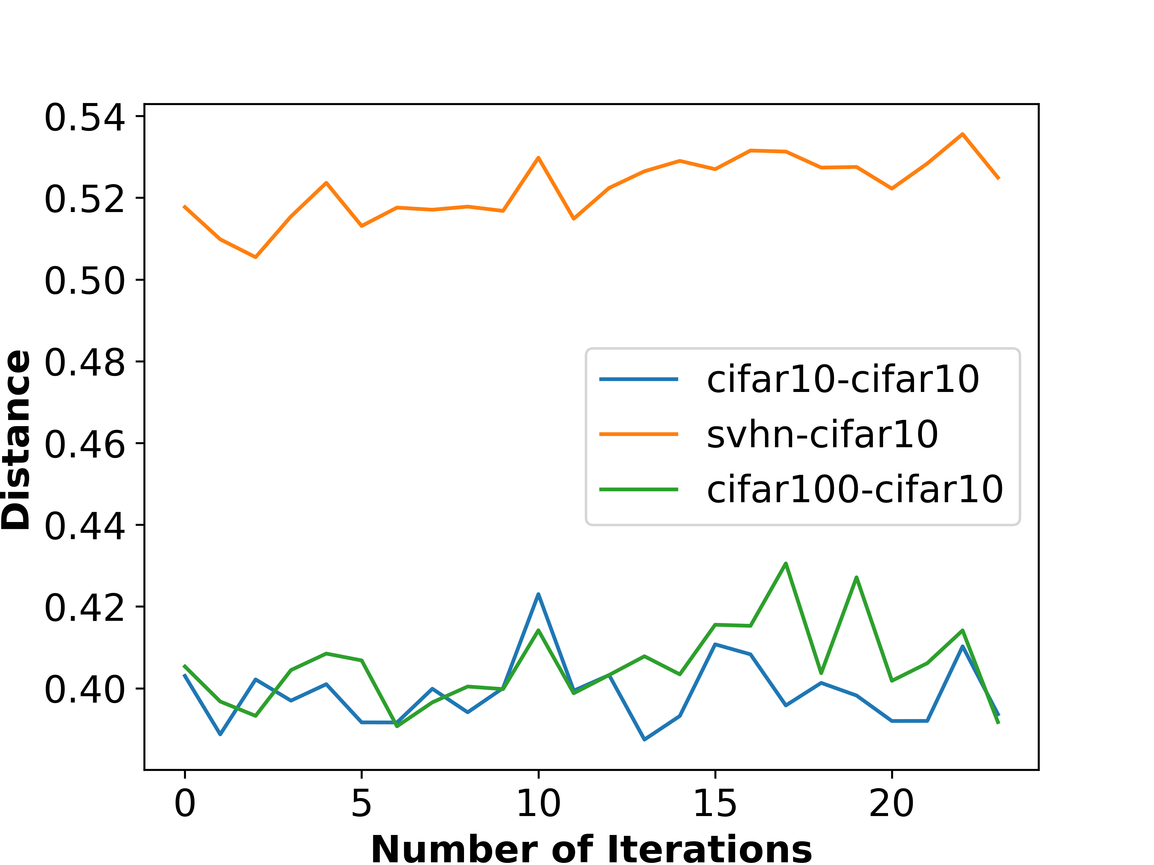
(a) Distance in 1 Epoch

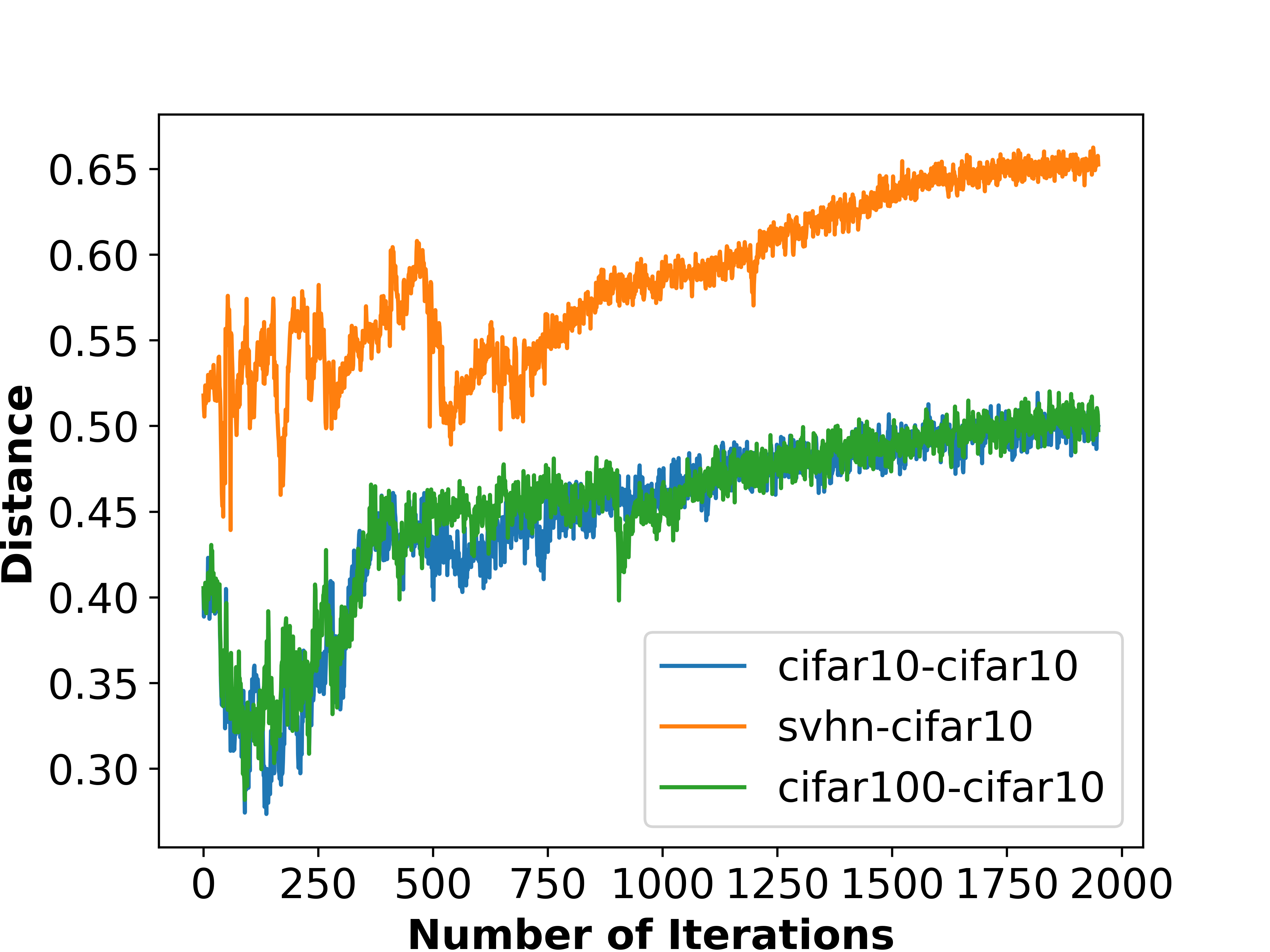
(b) Distance over 100 Epoch

Figure 1: The trend of distance during the process of training a ResNet20 model on CIFAR-10 using vanilla SGD. We follow a standard SGD training procedure and compute the distance between the current private batch and public examples at each iteration.

We empirically measure the GSD for each of the public datasets throughout the training process, as shown in Figure 1. This demonstrates that the relative ordering of the distances is preserved at almost all times. As a result, it suffices to compute each of the GSDs only once at initialization, requiring only one batch of examples from the private dataset and one pass through the model, incurring minimal data exposure and computational overhead. We can then select the dataset with the smallest GSD for use as our public dataset.

4.3 Private Distance Measurement

While Algorithm 1 has relatively low data exposure (requiring only a single batch of private examples), it is not differentially private. In this section, we give a general algorithm that computes GSD differential-privately: Differentially Private Gradient Subspace Distance (DP-GSD, Algorithm 2). As GSD needs top-$k$ singular vectors from private examples, we derive these singular vectors in a differentially private manner, and the rest of the algorithm remains DP because of post-processing.

Algorithm 2 Differentially Private Gradient Subspace Distance (DP-GSD)

  Input: $m$ private examples $x_{priv}$, $m$ public examples $x_{pub}$, loss function $\mathcal{L}$, model weights $\mathbf{w}_{0}$, dimension $k$, privacy parameter $\varepsilon,\delta$, clip norm $c$

  Output: Distance between two image datasets $\boldsymbol{d}$

1:  // Compute per-sample gradient matrix for private and public examples

2:  $G_{priv}=\nabla\mathcal{L}(\mathbf{w}_{0},x_{priv})$

3:  $G_{pub}=\nabla\mathcal{L}(\mathbf{w}_{0},x_{pub})$

4:  // Privately compute top-$k$ subspace of the private gradient matrix

5:  Clip per-row: $G_{priv}=\mathbf{Clip}(G_{priv},c)$

6:  Compute $V_{k}^{priv}\leftarrow\mathbf{DPPCA}(G_{priv},k,\varepsilon,\delta)$

7:  // Compute top-$k$ subspace of the public gradient matrix

8:  $U^{pub},S^{pub},V^{pub}\leftarrow\mathbf{SVD}(G_{pub})$

9:  // Compute the distance between two subspaces

10:  $\boldsymbol{d}=\mathbf{ProjectionMetric}(V_{k}^{priv},V_{k}^{pub})$

At a high level, DP-GSD makes one adaptation to GSD: we compute top-$k$ subspace of the private per-sample gradient matrix in a differentially private manner. $\mathbf{DPPCA}$ in line 6 of Algorithm 2 can be any Differentially Private Principle Component Analysis (DPPCA), e.g., input perturbation [dppca1], subspace perturbation [analysegauss], exponential mechanism [dppca1] and stochastic methods [liu2022dppca]. We give a theoretical analysis of the privacy and utility guarantee of DP-GSD based on the techniques of [dppca1], given in Algorithm 3.

Algorithm 3 Differentially Private Principle Component Analysis (DPPCA)

  Input: $m\times p$ data matrix $X$, dimension $k$, privacy parameter $\varepsilon$

  Output: $\hat{V}_{k}$: Top-$k$ subspace of $X$

1:  Set $A=\frac{1}{m}X^{\top}X$

2:  Sample $\hat{V}_{k}=\mathbf{BMF}\left(\frac{m\varepsilon}{2}A\right)$

To achieve DP, DPPCA randomly samples a $k$-dimensional distribution from the matrix Bingham distribution, which has the following density function:

$$f(V|A,k,p)=\frac{1}{{}_{1}F_{1}\left(\frac{1}{2}k,\frac{1}{2}p,A\right)}\exp\left(\operatorname{tr}\left(V^{T}AV\right)\right)$$ (11)

where $V$ is the $p\times k$ subspace and ${}_{1}F_{1}\left(\frac{1}{2}k,\frac{1}{2}p,A\right)$ is a normalization factor. We use $\mathbf{BMF}(V)$ in Algorithm 3 to denote this distribution. Thus, we have the following privacy and utility guarantees (proofs in Appendix D):

Theorem 2.

(Privacy Guarantee) Let Algorithm 3 be an implementation of $\mathbf{DPPCA}$ in DP-GSD, then DP-GSD is $\varepsilon/c^{2}$-differentially priate.

Theorem 3.

(Utility Guarantee) Let Algorithm 3 be an implementation of $\mathbf{DPPCA}$ in DP-GSD, then for $k=1$, the distance given by DP-GSD, $\hat{d}(V^{priv}_{k},V^{pub}_{k})$ is $(\rho,\eta)$-close to the distance given by GSD, $d(V^{priv}_{k},V^{pub}_{k})$, if we have

$$m>\frac{pc^{2}}{\varepsilon\alpha(1-\sqrt{1-\rho^{2}})}\left(4\frac{\log(1/\eta)}{p}+2\log\frac{8\lambda_{1}}{\rho^{2}\alpha}\right)$$ (12)

where $\lambda_{1}$ is the top eigenvalue, $\alpha=\lambda_{1}-\lambda_{2}$ is the eigen-gap, $p$ is the model dimension, $c$ is clip norm and $\varepsilon$ is the privacy parameter.

5 Second-Phase Pre-training

The standard method of private transfer learning consists of two phases: pre-training on a public dataset and fine-tuning on a private task. However, with large training sets and models, the computational burden of pre-training is prohibitive for most practitioners. Consequently, it is common to instead use pre-trained weights (obtained through pre-training on a fixed dataset) rather than run pre-training on a public dataset of choice. While this is computationally convenient, it limits the choice of pre-training datasets, and thus limits the accuracy in downstream fine-tuning.

$$\underbrace{f(\mathbf{W}_{0};x)\xrightarrow[]{\mathbf{X}^{pub,1}}f(\mathbf{W}_{PT};x)}_{\texttt{Load pre-trained weights}}\underbrace{\xrightarrow[\theta]{X_{pub,2}}f(\mathbf{W}_{PT},\theta_{0};x)}_{\texttt{Second-phase pre-training}}\underbrace{\xrightarrow[]{X_{priv}}f(\mathbf{W}_{PT},\hat{\theta};x)}_{\texttt{Private fine-tuning}}$$

Figure 2: Second-phase pre-training pipeline. We first choose a large model and download its pre-trained weights. Then we use an appropriate parameter-efficient fine-tuning mechanism and get trainable parameters $\theta$. We train $\theta$ on a public dataset and get $\theta_{0}$, called second-phase pre-training. Finally, we pass $\theta_{0}$ as the initial weights for private fine-tuning on the target task.

To alleviate this issue, we consider second-phase pre-training, in which a set of pre-trained weights are pre-trained on a second public dataset. We can then (privately) fine-tune the model on a sensitive dataset for the downstream task of interest. While this paradigm has previously been considered in the non-private setting [dontstop], to the best of our knowledge, we are the first to explore second phase pre-training in the differentially private setting. Pre-trained models may be significantly out of distribution with respect to the downstream task. Due to the noise introduced, the ability to adapt during fine-tuning may be diminished under differential privacy. Thus, the additional public data may be valuable for reducing the distribution shift. Second-phase pre-training is illustrated in Figure 2.

5.1 Second-Phase Pre-training Step by Step

Now we formally define second-phase pre-training. Suppose $f(\mathbf{W}_{pt};x)$ where $\mathbf{W}_{pt}$ denotes pre-trained weights and $x$ is input. To do second-phase pre-training, we first use a parameter-efficient fine-tuning mechanism and create new trainable parameters. Then we train these parameters on some public datasets. This step can be described by:

$$f_{2pt}\left(\mathbf{W}_{pt},\mathbf{\theta};x_{pub}\right)\rightarrow\mathbf{\theta}_{0}$$ (13)

where $x_{pub}$ are the public datasets and $\mathbf{\theta}$ are the new trainable parameters, which are of far lower dimensionality than $\mathbf{W}$. We get the parameter vector $\mathbf{\theta}_{0}$ after this second-phase pre-training step. Finally, we initialize $\mathbf{\theta}=\mathbf{\theta}_{0}$ and privately fine-tune it by running DPSGD on the private task:

$$f_{ft}\left(\mathbf{W}_{pt},\mathbf{\theta}_{0};x_{priv}\right)\rightarrow\hat{\mathbf{\theta}}$$ (14)

Our experiments show that second-phase pre-training can give additional accuracy improvements, even when we only have a small number of public data examples. Furthermore, our distance measurement GSD remains a good indicator for choosing good public data for the second phase pre-training.

5.2 Parameter Efficiency in Private Fine-tuning

In both private and non-private settings, approaches frequently depart from the default of fine-tuning all model weights. For example, one can freeze parameters and fine-tune only specific layers, or introduce new parameters entirely. The resulting number of tunable parameters is almost always chosen to be smaller than during pre-training, leading to parameter efficient methods. This can be beneficial in terms of portability and resource requirements, and the fine-tuned model utility frequently matches or compares favorably to full fine-tuning. Parameter efficiency may be further advantageous in the differentially private setting, as it reduces the magnitude of noise one must introduce (though findings on the downstream impact on utility remain inconclusive). In the settings we consider, we will empirically find that parameter-efficient methods result in better utility.

In general, there are two ways of parameter-efficient fine-tuning. One approach is to select a subset of layers or parameters for fine-tuning. For instance, [bias-term] proposed fine-tuning only the bias terms of a model, which is both computationally and parameter-efficient while retaining similar accuracy compared to other methods. Another study by [firstlast] found that fine-tuning the first and last layers of a model consistently improves its accuracy. The other approach is to freeze all existing parameters and add new trainable parameters during fine-tuning. Some examples include Adapter [adapter], Compacter [compacter] and LoRA [lora]. [YuNBGIKKLMWYZ22, LiTLH22] demonstrated that private fine-tuning using parameter-efficient methods on large language models can be both computationally efficient and accurate.

6 Experiments

We explore the predictive power of GSD in both pre-conditioning and transfer learning settings. Specifically, we use GSD to choose a public dataset for GEP [donot] (representative of pre-conditioning methods) and second-phase pre-training (representative of transfer learning settings). We use a variety of datasets, including Fashion MNIST [fmnist], SVHN [svhn], and CIFAR-10 [cifar10], as three canonical vision tasks. Based on the recommendations of [TramerKC22], we also evaluate our methods on datasets closer to privacy-sensitive applications. In particular, we also work with two medical image dataset: ChestX-ray14 [chestxray] and HAM10000 [ham]. A variety of datasets are chosen as public data respectively. We evaluate our algorithms using both CNN-based (e.g., ResNet152 [resnet], DenseNet121 [densenet]) and Transformer-based (ViTs [vit]) architectures. A variety of parameter-efficient fine-tuning mechanisms are considered, including freezing layers and LoRA [lora]. Further details on our experimental setup appear in Appendix B.

We compute GSD non-privately using Algorithm 1, for two reasons. First, as discussed in Section 4, the privacy leakage due to hyperparameter selection is considered to be minimal and often disregarded in private ML. We thus treat selection via GSD similarly. Second, beyond being a tool for public dataset selection, it is interesting in its own right to understand properties of GSD, including how it determines downstream utility across a variety of settings.

Ideally, we would like our distance measure GSD to be model agnostic: it should depend only the two datasets, not on any particular model. This is not the case, since, as stated, our algorithms take gradients of the two datasets on the model of interest. However, we show that GSD is robust to changes in model architecture. We evaluate GSD on a 2-layer CNN (which we call a “probe network”), and show that relative ordering of GSDs is preserved, even though the architecture is far simpler than the models of interest.

We also compare our algorithm with Task2Vec [task2vec], which has a similar goal as GSD. At a high level, Task2Vec represents a task (i.e., dataset) by transforming it into a vector so that the similarity between different datasets can be prescribed by the distance between two vectors. Although experiments show that Task2Vec matches taxonomic relations for datasets like iNaturalist [inatural], our empirical evaluation shows that it is outperformed by GSD in the differentially private setting.

6.1 Results for Pre-conditioning

We compute GSD and evaluate using GEP for the chosen datasets. The evaluation results are in Table 2. We find that, across several different private and public datasets, final accuracy is monotone as GSD decreases. Unexpectedly, we find that GSD between CIFAR-10 and CIFAR-100 is less than between CIFAR-10 and CIFAR-10. Nonetheless, this is predictive of final performance, where we see using CIFAR-100 as a public dataset is better than CIFAR-10, despite the fact that the private dataset is also CIFAR-10.

Table 2: GEP evaluation accuracy and corresponding distance in descending order. We use the same model for private training and GSD computation. ”-” means DP-SGD without public data.

. Accuracy Private Dataset Public Dataset Distance 58.63% CIFAR-10 CIFAR-100 0.20 57.64% CIFAR-10 0.24 56.75% SVHN 0.28 52.16% - - 91.32% SVHN SVHN 0.25 89.29% CIFAR-100 0.31 89.08% MNIST-M 0.39 83.21% - - 85.25% FMNIST FMNIST 0.34 84.54% FLOWER 0.43 83.91% MNIST 0.50 79.77% - -

For ChestX-ray14, we use AUC instead of prediction accuracy because of high class imbalance. The evaluation results are given in Table 1. Once again, lower GSD implies higher model utility. We see that ChestX-ray14 is the best public dataset, but the second best is another chest x-ray dataset. Furthermore, using a significantly different dataset (CIFAR-100) as the public dataset results in worse utility than using no public dataset at all. Therefore, it may be prudent for a practitioner to compute GSD in order to measure data suitability before proceeding to use it.

6.2 Results for Second-Phase Pre-training

Table 3: Second-Phase evaluation results and corresponding distance in descending order. We use DenseNet121 and choose two convolutional layers and the last layer for second-phase pre-training and private fine-tuning. Detailed settings can be found in Appendix B. We use the same model setting for private training and distance computation. ”-” means DP-SGD training.

. AUC Private Dataset Public Dataset Distance 87.06% HAM10000 HAM10000 0.50 85.53% KagSkin 0.68 85.40% - - 84.92% CIFAR-100 0.73 84.88% KagChest 0.73

We compute the GSD and evaluate using second-phase pre-training for the chosen datasets. The evaluation results are given in Table 3 and Table 4. As before, we consistently find that smaller GSD leads to larger utility. Like ChestX-ray14, HAM10000 is highly imbalanced, so we again use AUC. However, unlike ChestX-ray14, which contains roughly 100,000 images, HAM10000 is relatively small (only 10000 skin lesion images). We assume that we can only collect 300 images from it and treat them as public. As shown in Table 3, even this small public dataset can boost the utility through second-phase pre-training. While even the worst public dataset does not dramatically hurt utility (in contrast to the pre-conditioning setting), GSD can still be a good indicator of the utility of public datasets. Similar results apply when we evaluate second-phase pre-training and GSD on ChestX-ray14 using ViTs, as shown in Table 4.

Table 4: Second-Phase evaluation results and corresponding distance in descending order. We use ViT and LoRA fine-tuning. We use the same model setting for private training and distance computation. Detailed settings can be found in Appendix B. ”-” means DP-SGD training.

. AUC Private Dataset Public Dataset Distance 72.99% ChestX-ray14 ChestX-ray14 0.44 71.86% KagChest 0.59 70.93% - - 70.84% CIFAR-100 0.98

6.3 Transferability: Simple Models Remain Predictive

Table 5: Transferability evaluation results. The left-most column denotes each pair of private-public datasets, e.g. (Xray, Xray) means we take ChestX-ray14 as a private dataset, split part of its testset and take those images as public. Detailed settings can be found in Appendix B. The first row denotes different model architectures. ”Probe” is a simple CNN with around 30,000 parameters. ResNet152^∗ and ResNet152^∗∗ use different parameter-efficient fine-tuning settings. We use the same model for each Distance-Accuracy. The results show that this distance given by GSD is generally robust across different algorithms (pre-conditioning or second-phase pre-training) and different model architectures (from simple Probe to ViT). A smaller distance indicates that this public dataset is more similar to the private one, thus leveraging this public dataset for private learning will result in better accuracy.

Probe ResNet152^∗ ResNet152^∗∗ DenseNet121 ViT Task Pre-conditioning Second-phase Second-phase Second-phase Distance — Accuracy (Xray, Xray) 0.39 0.15 — 69.02% 0.31 — 67.48% 0.33 — 67.53% 0.44 — 72.99% (Xray, Chest) 0.52 0.36 — 66.62% 0.34 — 67.27% 0.37 — 67.40% 0.59 — 71.86% (Xray, CIFAR) 0.58 0.55 — 48.80% 0.39 — 66.57% 0.40 — 67.28% 0.98 — 70.84% (HAM, HAM) 0.42 - 0.48 — 86.83% 0.50 — 87.06% 0.50 — 84.94% (HAM, Skin) 0.55 - 0.65 — 85.95% 0.68 — 85.53% 0.76 — 81.23% (HAM, CIFAR) 0.67 - 0.70 — 85.49% 0.73 — 84.92% 0.97 — 77.07% (HAM, Chest) 0.76 - 0.70 — 85.41% 0.73 — 84.88% 0.93 — 78.65%

Our empirical evaluation suggests that GSD is transferable over different architectures. In previous experiments, we used the same model architecture for both GSD and the (private) learning algorithm. We find that the relative GSD ordering of different public datasets is robust across different architectures. For example, GSD(ChestX-ray14, KagChest) is consistently smaller than GSD(ChestX-ray14, CIFAR-100), no matter what model architecture or parameter-efficient fine-tuning mechanism we choose. Inspired by this finding, we measure GSD with a very simple CNN, which we call a “probe network.” It consists of two convolutional layers and one linear layer, with roughly 30,000 parameters. Evaluation results are given in Table 5. They demonstrate that even using a simple CNN, GSD can still derive accurate distance measurement with regard to the utility of public data for private learning tasks. The similarity described by GSD is thus robust against the choice of model architecture.

6.4 Task2Vec May Give Wrong Prediction

Result.

We evaluate the similarity between each public-private dataset pair using Task2Vec. Task2Vec gives similarity results of mixed quality: to highlight one notable failure case, we consider the ChestX-ray14 private dataset in Table 6. The closest dataset is itself. However, following this, CIFAR-100 is as close as KagChest, while it is qualitatively very different from ChestX-ray14 and provides low utility when used as the public dataset. In contrast, GSD orders the quality of these datasets in a manner consistent with their quality. We find similar discrepancies for HAM10000, results are given in the Appendix C.

Table 6: Results for GSD vs. Task2Vec. We evaluate ChestX-ray14 using GEP and compute the distance using Task2Vec and GSD. As suggested by Task2Vec, CIFAR-100 should be as close to ChestX-ray14 as KagChest, while it actually provides low utility.

	AUC	Task2Vec	GSD
ChestX-ray14	69.02%	0.052	0.15
KagChest	66.62%	0.16	0.36
-	64.90%	-	-
CIFAR-100	48.80%	0.16	0.55

7 Conclusion

A recent line of work explores the power of public data in private machine learning. However, evaluating the quality of the data is still a question that must be addressed. We propose a new distance GSD to predict utility of public datasets in private ML. We empirically demonstrate that lower GSD of a public dataset is strongly predictive of higher downstream utility. Our algorithms require minimal data and are computationally efficient. Additionally, transferability of GSD demonstrates that it is generally model agnostic, allowing one to decouple the public dataset selection and private learning. We further demonstrate that GSD is effective for predicting utility in settings involving both pre-conditioning and second-phase pre-training, and that GSD compares favorably to other measures of dataset distance.

Appendix A Missing Preliminaries

Gradient Embedding Perturbation (GEP).

Our theoretical analysis is based on GEP, the state-of-the-art private learning algorithm that leverages public data. Here we briefly introduce their algorithm. GEP involves three steps: 1) it computes a set of the orthonormal basis for the lower-dimensional subspace; 2) GEP projects the private gradients to the subspace derived from step 1, thus dividing the private gradients into two parts: embedding gradients that contain most of the information carried by the gradient, and the remainder are called residual gradients; 3) GEP clips two parts of the gradients separately and perturbs them to achieve differential privacy.

Algorithm 4 Gradient Embedding Perturbation (GEP)

  Input: Private dataset $X_{priv}$, public examples $x_{pub}$, loss function $\mathcal{L}$, model weights $\boldsymbol{\theta}_{0}$, dimension $k$, learning rate $\eta$, number of iterations $T$, noise multiplier $\sigma_{1},\sigma_{2}$, clip norm $S_{1},S_{2}$

  Output: Differentially private model $\boldsymbol{\theta}_{T}$

1:  for $t=1$ to $T$ do

2:     Compute per-sample gradient matrix $G^{priv}_{t}$ and public gradient matrix $G^{pub}_{t}$

3:     // Compute an orthonormal basis for the public subspace

4:     Initialize $V^{pub}_{k}\in\mathbb{R}^{k\times p}$ randomly.

5:     for $i=1$ to $T_{power}$ do

6:        Compute $A=G^{pub}_{t}V^{pub\top}_{k}$ and $V^{pub}_{k}=A^{\top}V^{pub\top}_{k}$

7:        Orthogonalize $V^{pub}_{k}$ and normalize row vectors.

8:     end for

9:     Delete $G^{pub}_{t}$ to free memory.

10:     // Project the private gradients onto public subspace

11:     Compute gradient embedding $W_{t}=G^{priv}_{t}V^{pub\top}_{k,t}$ and clip its rows with $S_{1}$ to obtain $\hat{W}$.

12:     Compute residual gradients $R_{t}=G^{priv}_{t}-W_{t}V^{pub}_{k,t}$ and clip its rows with $S_{2}$ to obtain $\hat{R}$.

13:     // Perturb gradient embedding and residual gradient separately

14:     Perturb embedding with noise $\boldsymbol{z}_{t}^{(1)}\sim\mathcal{N}\left(0,\sigma_{1}^{2}\boldsymbol{I}_{k\times k}\right)$: $w_{t}:=$sum over rows of $\hat{W}_{t}$, $\hat{w}_{t}:=w_{t}+\boldsymbol{z}_{t}^{(1)}$

15:     Perturb residual gradient with noise $\boldsymbol{z}_{t}^{(2)}\sim\mathcal{N}\left(0,\sigma_{2}^{2}\boldsymbol{I}_{k\times k}\right)$: $r_{t}:=$sum over rows of $\hat{R}_{t}$, $\hat{r}_{t}:=r_{t}+\boldsymbol{z}_{t}^{(2)}$

16:     $\hat{v}_{t}:=(\hat{w}_{t}^{\top}V^{pub}_{k}+\hat{r}_{t})/n$

17:     // Update weights

18:     $\boldsymbol{\theta}_{t+1}=\boldsymbol{\theta}_{t}-\eta\hat{v}_{t}$

19:  end for

Theorem 4.

(Theorem 3.2 in [donot]) GEP (Algorithm 4) is $(\varepsilon,\delta)-DP$ for any $\varepsilon<2\log(1/\delta)$ and $\delta\in(0,1)$ when $\sigma\geq 2\sqrt{2T\log(1/\delta)}/\varepsilon$.

Theorem 5.

(Theorem 3.3 in [donot]) Assume that the loss $L(\mathbf{w})=\frac{1}{n}\sum_{i=1}^{n}\ell\left(\mathbf{w},z_{i}\right)$ is 1-Lipschitz, convex, and $\beta$-smooth. Let $\mathbf{w}^{*}=\mathrm{argmin}_{w\in\mathcal{W}}L(\mathbf{w})$. The excess risk of GEP obeys

$$\mathbb{E}[L(\overline{\boldsymbol{\mathbf{w}}})]-L\left(\boldsymbol{\mathbf{w}}^{*}\right)\leq O\left(\frac{\sqrt{k\log(1/\delta)}}{n\varepsilon}\right)+O\left(\frac{\overline{r}\sqrt{p\log(1/\delta)}}{n\varepsilon}\right)$$ (15)

where $\eta=\frac{1}{\beta},T=\frac{n\beta\varepsilon}{\sqrt{p}}$, $\overline{\boldsymbol{\mathbf{w}}}=\frac{1}{T}\sum_{t=1}^{T}\mathbf{w}_{t}$, $\overline{r}=\frac{1}{T}\sum_{t=1}^{T}r^{2}_{t}$, $r_{t}=\|\mathbf{G}_{priv}-\mathbf{G}_{priv}V_{k}^{pub}V_{k}^{pub\top}\|_{2}$ is the reconstruction error at step t.

Appendix B Experiments Setting

Model Architecture.

As to pre-conditioning experiments, for Fashion MNIST, we use a simple convolutional neural network with around 26000 parameters as in Table 7a. For SVHN and CIFAR-10, we use ResNet20 which contains roughly 260,000 parameters. Batch normalization layers are replaced by group normalization layers for different private training, aligning with GEP settings. For ChestX-ray14, we use ResNet152 which has been pretrained on ImageNet1k, a subset of the full ImageNet [imagenet] dataset. We privately fine-tune its classification layer, which contains around 28,000 parameters. We use the same model architecture for subspace distance computation and GEP private training. As to second-phase experiments, we evaluate ChestX-ray14, HAM10000 on ResNet152, DenseNet121, and ViT using various parameter-efficient fine-tuning techniques, we list them in Table 8. We use a simple 2-layer CNN for the probe network, shown in Table 7b.

Table 7: Self-designed model architectures.

.

Layer	Parameters
Conv2d	16 filters of 8x8, stride=2
Maxpooling2d	stride=2
Conv2d	32 filters 4x4, stride=2
Linear	32 units
Softmax	10 units

(a) Model architecture for Fashion MNIST.

Layer	Parameters
Conv2d	64 filters of 8x8, stride=5
Maxpooling2d	stride=2
Conv2d	16 filters 4x4, stride=3
Maxpooling2d	stride=2
Linear	144 units
Sigmoid	num_classes

(b) Model architecture for Probe Network.

Table 8: Parameter-efficient fine-tuning mechanisms for different models.

. Model Fine-tuning mechanism ResNet152 fc + layer3.32.conv1.weight DenseNet121 classifier + features.denseblock3.denselayer23.conv1.weight + features.denseblock3.denselayer24.conv1.weight ViT LoRA ($\alpha=8,r=8$)

Table 9: Choices of public dataset for private dataset. The four datasets in the first row are private datasets. The datasets listed in the first columns are choices of public datasets. ’X’ means we choose the two corresponding datasets as a pair of private/public dataset.

. CIFAR-10 SVHN Fashion MNIST ChestX-ray14 HAM10000 CIFAR-10 X CIFAR-100 X X X X SVHN X X MNIST_M X Fashion MNIST X FLOWER X MNIST X ChestX-ray14 X KagChest X X HAM10000 X KagSkin X

Dataset Choice.

CIFAR-10, SVHN and Fashion MNIST are commonly used for evaluation purposes in Computer Vision. ChestX-ray14 consists of frontal view X-ray images with 14 different classes of lung disease. In our evaluation, there are 78,466 training examples and 20433 testing examples in ChestX-ray14. HAM10000 is composed of 10,000 dermatoscopic images of pigmented lesions. Our choices of public datasets for the four private datasets are described in Table 9. Among them, MNIST-M [mnistm] consists of MNIST digits placed on randomly selected backgrounds taken from color photos in the BSDS500 dataset. FLOWER [flower] consists of 102 flower categories. KagChest [kagchest] imagees were selected from retrospective cohorts of pediatric patients of one to five years old from Guangzhou Women and Children’s Medical Center, Guangzhou. It is easy to be obtained from Kaggle so we name it KagChest. Similarly for the KagSkin [kagskin], which images of benign skin moles and malignant skin moles. We split the first 300 (for ChestX-ray14, this number is 2000) images in the testset and take them as public. The next 300 (again, for ChestX-ray14, this number is 2000) images are the chose private examples.

Hyperparameter Setting.

We use $\varepsilon=2$ and $\delta=1e-5$ for all the evaluations. For distance computation, we choose $k=16$. We follow the hyperparameter setting in the GEP paper for evaluation. In the GEP paper, they didn’t evaluate GEP on the ChestX-ray14 dataset. In our evaluation, we choose $k=100$ and clip norms are 3 and 1 for original and residual gradients, respectively. The learning rate for the SGD optimizer is set to 0.05. All other hyperparameters are set as default. For second-phase pre-training, we use those public examples to perform supervised learning on trainable parameters. We use Adam optimizer and set $\eta=3e-3$ for Transformer-based models and $\eta=5e-5$ for CNN-based models. For private fine-tuning, we use SGD optimizer and set $\eta=0.8$ and clip norm $=0.1$.

Appendix C More Experiments

C.1 Gradients are in a lower-dimensional subspace.

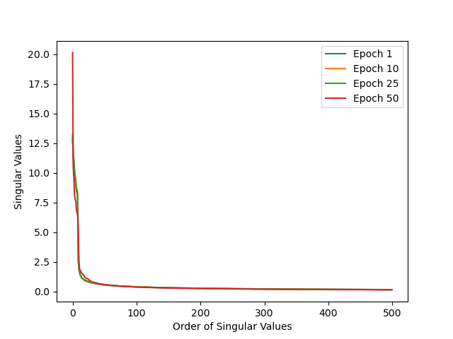
(a) CIFAR-10

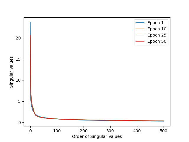
(b) ChestX-ray14

Figure 3: Top 500 singular values in the training procedure using vanilla SGD. Model architectures are in the Appendix B. Only a small fraction of singular values are extremely large while the rest are close to 0, meaning that most of the gradients lie in a lower-dimensional subspace, which corresponds to the top singular vectors.

.

We evaluate the empirical observation that the stochastic gradients stay in a lower-dimensional subspace during the training procedure of a deep learning model [subspace1, subspace2], as shown in Figure 3b. Results show that only a tiny fraction of singular values are enormous. At the same time, the rest are close to 0, meaning that most of the gradients lie in a lower-dimensional subspace, corresponding to the top singular vectors.

C.2 More Second-Phase Pre-training Evaluation.

We evaluate second-phase pre-training and GSD on ChestX-ray14 and HAM10000 using ResNet152, DenseNet121, and ViT. Aside from the results we presented, we show the rest of the results here.

Table 10: Second-Phase evaluation results and corresponding distance on ChestX-ray14 in descending order. Detailed settings can be found in Appendix B. We use the same model setting for private training and distance computation. ”-” means vanilla DP-SGD training.

AUC	Private Dataset	Public Dataset	Distance
67.48%	ChestX-ray14	ChestX-ray14	0.31
67.27%		KagChest	0.34
66.82%		-	-
66.57%		CIFAR-100	0.39

(a) ResNet152

AUC	Private Dataset	Public Dataset	Distance
67.53%	ChestX-ray14	ChestX-ray14	0.33
67.47%		-	-
67.40%		KagChest	0.37
67.28%		CIFAR-100	0.40

(b) DenseNet121

Table 11: Second-Phase evaluation results and corresponding distance on HAM10000 in descending order. Detailed settings can be found in Appendix B. We use the same model setting for private training and distance computation. ”-” means vanilla DP-SGD training.

AUC	Private Dataset	Public Dataset	Distance
86.83%	HAM10000	HAM10000	0.48
85.95%		KagSkin	0.65
85.55%		-	-
85.49%		CIFAR-100	0.70
85.41%		KagChest	0.70

(a) ResNet152

AUC	Private Dataset	Public Dataset	Distance
84.94%	HAM10000	HAM10000	0.50
81.23%		KagSkin	0.76
78.65%		KagChest	0.93
77.07%		CIFAR-100	0.97
73.67%		-	-

(b) ViT

C.3 More vs. Task2Vec.

We evaluate the similarity between each public-private dataset pair using Task2Vec. The results on HAM10000 public dataset are presented here using cluster map in Figure 4. The closest datasets are itself, and the HAM10000 public dataset. However, following this, the closest dataset is KagChest, which is qualitatively very different from HAM10000 (chest x-rays versus skin lesions) and provides low utility when used as the public dataset (see Table 5). In particular, KagSkin (another skin disease dataset) is qualitatively closer to HAM10000 and provides higher utility when used as a public dataset, yet Task2Vec assigns it a greater distance than KagChest. In contrast, GSD orders the quality of these datasets in a manner consistent with their quality.

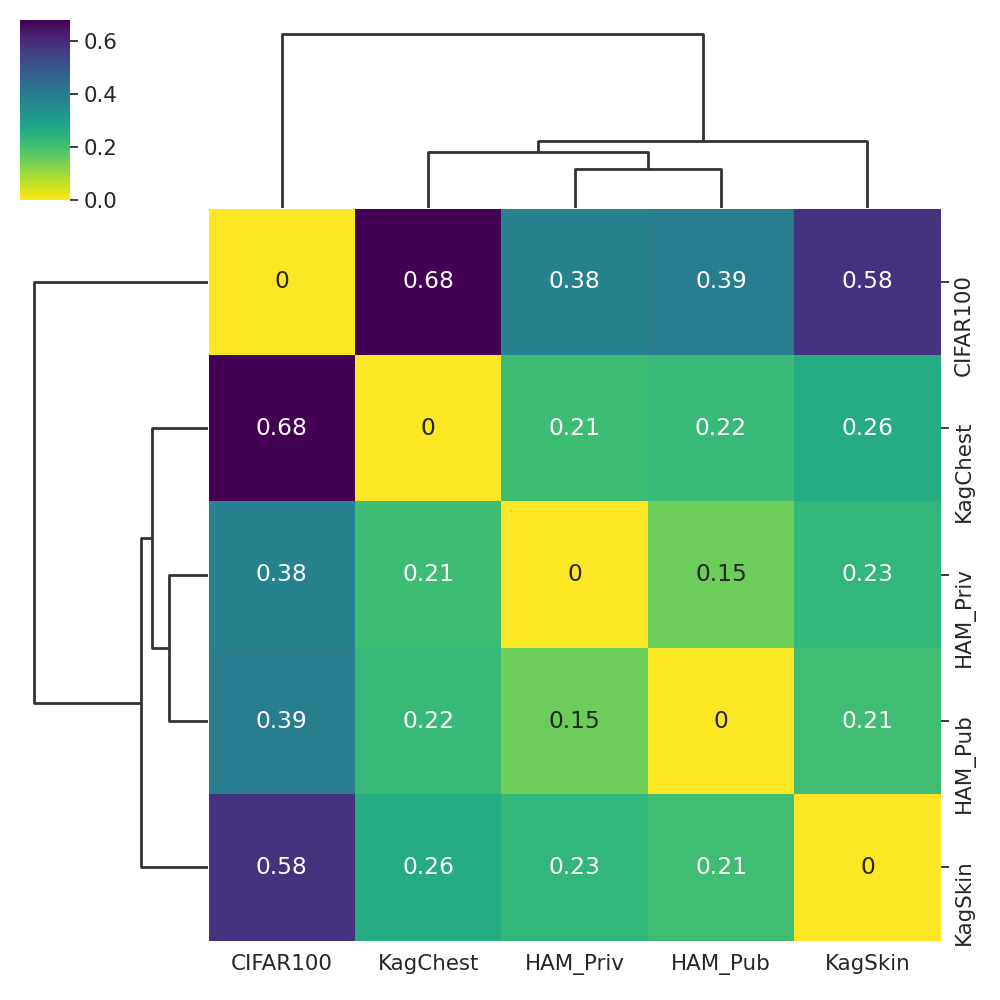
(a) Clustermap given by Task2Vec

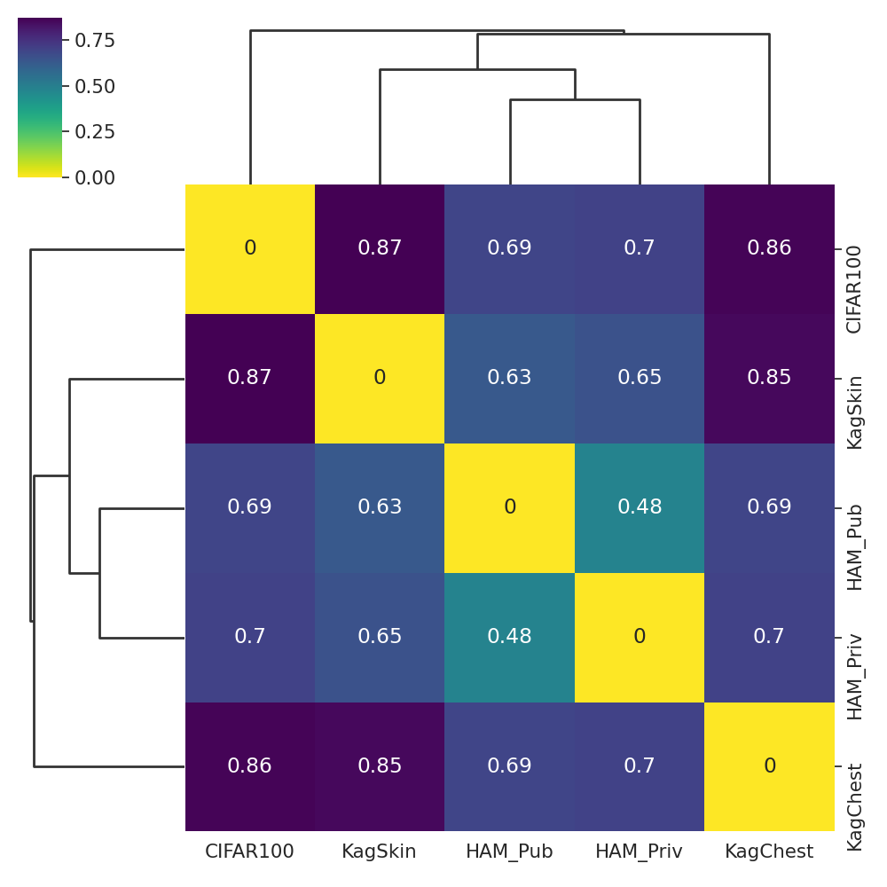
(b) Clustermap given by GSD

Figure 4: Clustermaps given by Task2Vec (left) and GSD(right) for HAM10000 and corresponding public datasets. The lines on the top and the left denote the similarity of a pair of datasets. The numbers in the grid are the similarity distance for a pair of datasets. Although Task2Vec gives the correct prediction for (HAM_public, HAM_private) pair, it incorrectly predicts the second-close similarity, where it believes KagChest is the second-close dataset for HAM10000, while they should be totally irrelevant.

Appendix D Missing Proofs

In this section, we present proofs from Section 4.3.

Algorithm 5 Differentially Private Gradient Subspace Distance (DP-GSD)

  Input: $m$ private examples $x_{priv}$, $m$ public examples $x_{pub}$, loss function $\mathcal{L}$, model weights $\mathbf{w}_{0}$, dimension $k$, privacy parameter $\varepsilon,\delta$, clip norm $c$

  Output: Distance between two image datasets $\boldsymbol{d}$

1:  // Compute per-sample gradient matrix for private and public examples

2:  $G_{priv}=\nabla\mathcal{L}(\mathbf{w}_{0},x_{priv})$

3:  $G_{pub}=\nabla\mathcal{L}(\mathbf{w}_{0},x_{pub})$

4:  // Privately compute top-$k$ subspace of the private gradient matrix

5:  Clip per-row: $G_{priv}=\mathbf{Clip}(G_{priv},c)$

6:  Compute $V_{k}^{priv}\leftarrow\mathbf{DPPCA}(G_{priv},k,\varepsilon,\delta)$

7:  // Compute top-$k$ subspace of the public gradient matrix

8:  $U^{pub},S^{pub},V^{pub}\leftarrow\mathbf{SVD}(G_{pub})$

9:  // Compute the distance between two subspaces

10:  $\boldsymbol{d}=\mathbf{ProjectionMetric}(V_{k}^{priv},V_{k}^{pub})$

Algorithm 6 Differentially Private Principle Component Analysis (DPPCA)

  Input: $m\times p$ data matrix $X$, dimension $k$, privacy parameter $\varepsilon$

  Output: $\hat{V}_{k}$: Top-$k$ subspace of $X$

1:  Set $A=\frac{1}{m}X^{\top}X$

2:  Sample $\hat{V}_{k}=\mathbf{BMF}\left(\frac{m\varepsilon}{2}A\right)$

Lemma 2.

(Theorem 6 in [dppca1]) DPPCA (Algorthim 3) is $\varepsilon$-differentially private.

Theorem 2 (Privacy Guarantee).

Let Algorithm 3 be an implementation of $\mathbf{DPPCA}$ in DP-GSD, then DP-GSD is $\varepsilon/c^{2}$-differentially priate.

Proof.

Let $x_{priv}$ be $m$ private examples. $G_{priv}=\mathbf{Clip}(\nabla\mathcal{L}(\mathbf{w}_{0},x_{priv}),c)\in\mathcal{R}^{m\times p}$ is per-sample gradient matrix and $A=\frac{1}{m}G_{priv}G_{priv}^{\top}$. We sample top-$k$ eigenvectors from the matrix Bingham distribution [matrixbingham]:

$$f(V|A,k,p)=\frac{1}{{}_{1}F_{1}\left(\frac{1}{2}k,\frac{1}{2}p,A\right)}\exp\left(\operatorname{tr}\left(V^{T}AV\right)\right)$$ (16)

with $A=\frac{m\varepsilon}{2c^{2}}A$. We show that this is the exponential mechanism applied to the score function $q(V;x)=mv^{T}Av$.

Consider the neighboring data $X^{\prime}_{priv}=[x_{1},...,x^{\prime}_{i},...,x_{m}]$ that differ from $X_{priv}$ with one data example $x^{\prime}_{i}$. Let $G^{\prime}_{priv}=\mathbf{Clip}(\nabla\mathcal{L}(\mathbf{w}_{0},x^{\prime}_{priv}),c)$ and $A^{\prime}=\frac{1}{m}G_{priv}^{{}^{\prime}\top}G^{\prime}_{priv}$. We have

$$\Delta q=\max\left|mv^{T}Av-mv^{T}A^{\prime}v\right| \leq\left|v^{T}(g_{i}g_{i}^{T}-g^{\prime}_{i}g^{{}^{\prime}\top}_{i})v\right|$$ (17)

$$\leq\left\|v^{T}g_{i}|\|^{2}-\|v^{T}g^{\prime}_{i}\|^{2}\right|$$

$$\leq\left\|v^{T}\nabla\mathcal{L}(\mathbf{w}_{0},x_{i})|\|^{2}-\|v^{T}\nabla\mathcal{L}(\mathbf{w}_{0},x^{\prime}_{i})\|^{2}\right|$$

$$\leq c^{2}$$

Therefore, from 2, we know that $\mathbf{DPPCA}$ in DP-GSD (Algorithm 2) is $\varepsilon/c^{2}$-differentially private. Thus, DP-GSD is $\varepsilon/c^{2}$-differentially private because of post-processing. ∎

Lemma 3.

(Theorem 7 in [dppca1]) Let $k=1$, the private gradient subspace $V^{priv}_{k}$ in GSD and the private gradient subspace $\hat{V}^{priv}_{k}$ from Algorithm 3 satisfy

$$\operatorname{Pr}\left(\left|\left\langle V^{priv}_{k},\hat{V}^{priv}_{k}\right\rangle\right|>\rho\right)\geq 1-\eta$$ (18)

if we have

$$m>\frac{p}{\varepsilon\alpha(1-\rho)}\left(4\frac{\log(1/\eta)}{p}+2\log\frac{8\lambda_{1}}{\left(1-\rho^{2}\right)\alpha}\right)$$ (19)

where $\lambda_{1}$ is the top eigenvalue, $\alpha=\lambda_{1}-\lambda_{2}$ is the eigen-gap, $p$ is the model dimension and $\varepsilon$ is the privacy parameter.

Theorem 3 (Utility Guarantee)

Let Algorithm 3 be an implementation of $\mathbf{DPPCA}$ in DP-GSD, then for $k=1$, the distance given by DP-GSD, $\hat{d}(V^{priv}_{k},V^{pub}_{k})$ is $(\rho,\eta)$-close to the distance given by GSD, $d(V^{priv}_{k},V^{pub}_{k})$, if we have

$$m>\frac{pc^{2}}{\varepsilon\alpha(1-\sqrt{1-\rho^{2}})}\left(4\frac{\log(1/\eta)}{p}+2\log\frac{8\lambda_{1}}{\rho^{2}\alpha}\right)$$ (20)

where $\lambda_{1}$ is the top eigenvalue, $\alpha=\lambda_{1}-\lambda_{2}$ is the eigen-gap, $p$ is the model dimension, $c$ is clip norm and $\varepsilon$ is the privacy parameter.

Proof.

Let $V^{priv}_{k}$ be the private gradient subspace in GSD and $\hat{V}^{priv}_{k}$ be the private gradient subspace in DP-GSD, $d(V^{priv}_{k},\hat{V}^{priv}_{k})$ be the projection metric distance between two subspaces. From Lemma 3, we have

$$\operatorname{Pr}\left(\left|\left\langle V^{priv}_{k},\hat{V}^{priv}_{k}\right\rangle\right|>\mu\right)=\operatorname{Pr}\left(d(V^{priv}_{k},\hat{V}^{priv}_{k})\leq\sqrt{1-\rho^{2}}\right)\geq 1-\eta$$ (21)

$$\xrightarrow[]{(a)}\operatorname{Pr}\left(\left|\hat{d}(V^{priv}_{k},V^{pub}_{k})-d(V^{priv}_{k},V^{pub}_{k})\right|\leq\sqrt{1-\mu^{2}}\right)\geq 1-\eta$$

(a) holds because of the triangle inequality of projection metric [projectionmetric]. Substituting $\sqrt{1-\mu^{2}}$ with $\rho$, we have $\hat{d}(V^{priv}_{k},V^{pub}_{k})$ is $(\rho,\eta)$-close to $d(V^{priv}_{k},V^{pub}_{k})$. ∎

References

- [ACG+16] Martin Abadi, Andy Chu, Ian Goodfellow, H. Brendan McMahan, Ilya Mironov, Kunal Talwar, and Li Zhang. Deep learning with differential privacy. In Proceedings of the 2016 ACM SIGSAC Conference on Computer and Communications Security, CCS ’16, page 308–318, New York, NY, USA, 2016. Association for Computing Machinery.
- [ALT+19] Alessandro Achille, Michael Lam, Rahul Tewari, Avinash Ravichandran, Subhransu Maji, Charless C. Fowlkes, Stefano Soatto, and Pietro Perona. Task2vec: Task embedding for meta-learning. In 2019 IEEE/CVF International Conference on Computer Vision, ICCV 2019, Seoul, Korea (South), October 27 - November 2, 2019, pages 6429–6438. IEEE, 2019.
- [BBC+10] Shai Ben-David, John Blitzer, Koby Crammer, Alex Kulesza, Fernando Pereira, and Jennifer Wortman Vaughan. A theory of learning from different domains. Mach. Learn., 79(1-2):151–175, 2010.
- [BBCP06] Shai Ben-David, John Blitzer, Koby Crammer, and Fernando Pereira. Analysis of representations for domain adaptation. In Bernhard Schölkopf, John C. Platt, and Thomas Hofmann, editors, Advances in Neural Information Processing Systems 19, Proceedings of the Twentieth Annual Conference on Neural Information Processing Systems, Vancouver, British Columbia, Canada, December 4-7, 2006, pages 137–144. MIT Press, 2006.
- [BST14] Raef Bassily, Adam D. Smith, and Abhradeep Thakurta. Private empirical risk minimization: Efficient algorithms and tight error bounds. In 55th IEEE Annual Symposium on Foundations of Computer Science, FOCS 2014, Philadelphia, PA, USA, October 18-21, 2014, pages 464–473. IEEE Computer Society, 2014.
- [BWZK22] Zhiqi Bu, Yu-Xiang Wang, Sheng Zha, and George Karypis. Differentially private bias-term only fine-tuning of foundation models, 2022.
- [CCCPT22] Yannis Cattan, Christopher A. Choquette-Choo, Nicolas Papernot, and Abhradeep Thakurta. Fine-tuning with differential privacy necessitates an additional hyperparameter search, 2022.
- [Chi03] Yasuko Chikuse. Statistics on special manifolds, volume 174. Springer Science & Business Media, 2003.
- [CHS02] J. H. Conway, R. H. Hardin, and N. J. A. Sloane. Packing lines, planes, etc.: Packings in grassmannian space. 2002.
- [CSS13] Kamalika Chaudhuri, Anand D. Sarwate, and Kaushik Sinha. A near-optimal algorithm for differentially-private principal components. J. Mach. Learn. Res., 14(1):2905–2943, 2013.
- [CTW+21] Nicholas Carlini, Florian Tramèr, Eric Wallace, Matthew Jagielski, Ariel Herbert-Voss, Katherine Lee, Adam Roberts, Tom Brown, Dawn Song, Úlfar Erlingsson, Alina Oprea, and Colin Raffel. Extracting training data from large language models. In 30th USENIX Security Symposium (USENIX Security 21), pages 2633–2650. USENIX Association, August 2021.
- [DBH+22] Soham De, Leonard Berrada, Jamie Hayes, Samuel L Smith, and Borja Balle. Unlocking high-accuracy differentially private image classification through scale. arXiv preprint arXiv:2204.13650, 2022.
- [DBK+20] Alexey Dosovitskiy, Lucas Beyer, Alexander Kolesnikov, Dirk Weissenborn, Xiaohua Zhai, Thomas Unterthiner, Mostafa Dehghani, Matthias Minderer, Georg Heigold, Sylvain Gelly, Jakob Uszkoreit, and Neil Houlsby. An image is worth 16x16 words: Transformers for image recognition at scale. CoRR, abs/2010.11929, 2020.
- [DDS+09] J. Deng, W. Dong, R. Socher, L.-J. Li, K. Li, and L. Fei-Fei. ImageNet: A Large-Scale Hierarchical Image Database. In CVPR09, 2009.
- [DMNS06] Cynthia Dwork, Frank McSherry, Kobbi Nissim, and Adam Smith. Calibrating noise to sensitivity in private data analysis. In Shai Halevi and Tal Rabin, editors, Theory of Cryptography, pages 265–284, Berlin, Heidelberg, 2006. Springer Berlin Heidelberg.
- [DTTZ14] Cynthia Dwork, Kunal Talwar, Abhradeep Thakurta, and Li Zhang. Analyze gauss: optimal bounds for privacy-preserving principal component analysis. In David B. Shmoys, editor, Symposium on Theory of Computing, STOC 2014, New York, NY, USA, May 31 - June 03, 2014, pages 11–20. ACM, 2014.
- [EAS98] Alan Edelman, Tomás A. Arias, and Steven Thomas Smith. The geometry of algorithms with orthogonality constraints. SIAM J. Matrix Anal. Appl., 20(2):303–353, 1998.
- [EY36] Carl Eckart and Gale Young. The approximation of one matrix by another of lower rank. Psychometrika, 1(3):211–218, 1936.
- [Fan19] Claudio Fanconi. Skin cancer: Malignant vs. benign, June 2019.
- [FJR15] Matt Fredrikson, Somesh Jha, and Thomas Ristenpart. Model inversion attacks that exploit confidence information and basic countermeasures. In Proceedings of the 22nd ACM SIGSAC Conference on Computer and Communications Security, CCS ’15, page 1322–1333, New York, NY, USA, 2015. Association for Computing Machinery.
- [GAW+22] Aditya Golatkar, Alessandro Achille, Yu-Xiang Wang, Aaron Roth, Michael Kearns, and Stefano Soatto. Mixed differential privacy in computer vision. CoRR, abs/2203.11481, 2022.
- [GL96] Gene H. Golub and Charles F. Van Loan. Matrix Computations, Third Edition. Johns Hopkins University Press, 1996.
- [GMS+20] Suchin Gururangan, Ana Marasovic, Swabha Swayamdipta, Kyle Lo, Iz Beltagy, Doug Downey, and Noah A. Smith. Don’t stop pretraining: Adapt language models to domains and tasks. In Dan Jurafsky, Joyce Chai, Natalie Schluter, and Joel R. Tetreault, editors, Proceedings of the 58th Annual Meeting of the Association for Computational Linguistics, ACL 2020, Online, July 5-10, 2020, pages 8342–8360. Association for Computational Linguistics, 2020.
- [GMT14] Virginie Gabrel, Cécile Murat, and Aurélie Thiele. Recent advances in robust optimization: An overview. European journal of operational research, 235(3):471–483, 2014.
- [GRD18] Guy Gur-Ari, Daniel A. Roberts, and Ethan Dyer. Gradient descent happens in a tiny subspace. CoRR, abs/1812.04754, 2018.
- [GUA+16] Yaroslav Ganin, Evgeniya Ustinova, Hana Ajakan, Pascal Germain, Hugo Larochelle, François Laviolette, Mario Marchand, and Victor S. Lempitsky. Domain-adversarial training of neural networks. J. Mach. Learn. Res., 17:59:1–59:35, 2016.
- [HAS+18] Grant Van Horn, Oisin Mac Aodha, Yang Song, Yin Cui, Chen Sun, Alexander Shepard, Hartwig Adam, Pietro Perona, and Serge J. Belongie. The inaturalist species classification and detection dataset. In 2018 IEEE Conference on Computer Vision and Pattern Recognition, CVPR 2018, Salt Lake City, UT, USA, June 18-22, 2018, pages 8769–8778. Computer Vision Foundation / IEEE Computer Society, 2018.
- [HGJ+19] Neil Houlsby, Andrei Giurgiu, Stanislaw Jastrzebski, Bruna Morrone, Quentin De Laroussilhe, Andrea Gesmundo, Mona Attariyan, and Sylvain Gelly. Parameter-efficient transfer learning for NLP. In Kamalika Chaudhuri and Ruslan Salakhutdinov, editors, Proceedings of the 36th International Conference on Machine Learning, volume 97 of Proceedings of Machine Learning Research, pages 2790–2799. PMLR, 09–15 Jun 2019.
- [HL08] Jihun Ham and Daniel D. Lee. Grassmann discriminant analysis: a unifying view on subspace-based learning. In William W. Cohen, Andrew McCallum, and Sam T. Roweis, editors, Machine Learning, Proceedings of the Twenty-Fifth International Conference (ICML 2008), Helsinki, Finland, June 5-9, 2008, volume 307 of ACM International Conference Proceeding Series, pages 376–383. ACM, 2008.
- [HLvdMW17] Gao Huang, Zhuang Liu, Laurens van der Maaten, and Kilian Q. Weinberger. Densely connected convolutional networks. In 2017 IEEE Conference on Computer Vision and Pattern Recognition, CVPR 2017, Honolulu, HI, USA, July 21-26, 2017, pages 2261–2269. IEEE Computer Society, 2017.
- [HysW+22] Edward J Hu, yelong shen, Phillip Wallis, Zeyuan Allen-Zhu, Yuanzhi Li, Shean Wang, Lu Wang, and Weizhu Chen. LoRA: Low-rank adaptation of large language models. In International Conference on Learning Representations, 2022.
- [HZRS16] Kaiming He, Xiangyu Zhang, Shaoqing Ren, and Jian Sun. Deep residual learning for image recognition. In 2016 IEEE Conference on Computer Vision and Pattern Recognition, CVPR 2016, Las Vegas, NV, USA, June 27-30, 2016, pages 770–778. IEEE Computer Society, 2016.
- [KGC+18] Daniel S. Kermany, Michael Goldbaum, Wenjia Cai, Carolina C.S. Valentim, Huiying Liang, Sally L. Baxter, Alex McKeown, Ge Yang, Xiaokang Wu, Fangbing Yan, Justin Dong, Made K. Prasadha, Jacqueline Pei, Magdalene Y.L. Ting, Jie Zhu, Christina Li, Sierra Hewett, Jason Dong, Ian Ziyar, Alexander Shi, Runze Zhang, Lianghong Zheng, Rui Hou, William Shi, Xin Fu, Yaou Duan, Viet A.N. Huu, Cindy Wen, Edward D. Zhang, Charlotte L. Zhang, Oulan Li, Xiaobo Wang, Michael A. Singer, Xiaodong Sun, Jie Xu, Ali Tafreshi, M. Anthony Lewis, Huimin Xia, and Kang Zhang. Identifying medical diagnoses and treatable diseases by image-based deep learning. Cell, 172(5):1122–1131.e9, 2018.
- [KH+09] Alex Krizhevsky, Geoffrey Hinton, et al. Learning multiple layers of features from tiny images. 2009.
- [KRRT20] Peter Kairouz, Mónica Ribero, Keith Rush, and Abhradeep Thakurta. Dimension independence in unconstrained private ERM via adaptive preconditioning. CoRR, abs/2008.06570, 2020.
- [KRRT21] Peter Kairouz, Mónica Ribero, Keith Rush, and Abhradeep Thakurta. (nearly) dimension independent private ERM with adagrad rates via publicly estimated subspaces. In Proceedings of the 34th Annual Conference on Learning Theory, COLT ’21, pages 2717–2746, 2021.
- [LGZ+20] Xinyan Li, Qilong Gu, Yingxue Zhou, Tiancong Chen, and Arindam Banerjee. Hessian based analysis of SGD for deep nets: Dynamics and generalization. In Carlotta Demeniconi and Nitesh V. Chawla, editors, Proceedings of the 2020 SIAM International Conference on Data Mining, SDM 2020, Cincinnati, Ohio, USA, May 7-9, 2020, pages 190–198. SIAM, 2020.
- [LKJO22] Xiyang Liu, Weihao Kong, Prateek Jain, and Sewoong Oh. DP-PCA: Statistically optimal and differentially private PCA. In Alice H. Oh, Alekh Agarwal, Danielle Belgrave, and Kyunghyun Cho, editors, Advances in Neural Information Processing Systems, 2022.
- [LLH+22] Xuechen Li, Daogao Liu, Tatsunori Hashimoto, Huseyin A. Inan, Janardhan Kulkarni, Yin Tat Lee, and Abhradeep Guha Thakurta. When does differentially private learning not suffer in high dimensions? CoRR, abs/2207.00160, 2022.
- [LTLH22] Xuechen Li, Florian Tramèr, Percy Liang, and Tatsunori Hashimoto. Large language models can be strong differentially private learners. In Proceedings of the 10th International Conference on Learning Representations, ICLR ’22, 2022.
- [LWAF21] Zelun Luo, Daniel J. Wu, Ehsan Adeli, and Li Fei-Fei. Scalable differential privacy with sparse network finetuning. In IEEE Conference on Computer Vision and Pattern Recognition, CVPR 2021, virtual, June 19-25, 2021, pages 5059–5068. Computer Vision Foundation / IEEE, 2021.
- [MHR21] Rabeeh Karimi Mahabadi, James Henderson, and Sebastian Ruder. Compacter: Efficient low-rank hypercomplex adapter layers. In Marc’Aurelio Ranzato, Alina Beygelzimer, Yann N. Dauphin, Percy Liang, and Jennifer Wortman Vaughan, editors, Advances in Neural Information Processing Systems 34: Annual Conference on Neural Information Processing Systems 2021, NeurIPS 2021, December 6-14, 2021, virtual, pages 1022–1035, 2021.
- [MSH+22] Shubhankar Mohapatra, Sajin Sasy, Xi He, Gautam Kamath, and Om Thakkar. The role of adaptive optimizers for honest private hyperparameter selection. In Proceedings of the Thirty-Sixth AAAI Conference on Artificial Intelligence, volume 36 of AAAI ’22, pages 7806–7813, 2022.
- [MTKC22] Harsh Mehta, Abhradeep Thakurta, Alexey Kurakin, and Ashok Cutkosky. Large scale transfer learning for differentially private image classification. arXiv preprint arXiv:2205.02973, 2022.
- [NWC+11] Yuval Netzer, Tao Wang, Adam Coates, Alessandro Bissacco, Bo Wu, and Andrew Y Ng. Reading digits in natural images with unsupervised feature learning. 2011.
- [NZ08] Maria-Elena Nilsback and Andrew Zisserman. Automated flower classification over a large number of classes. In Indian Conference on Computer Vision, Graphics and Image Processing, Dec 2008.
- [PS22] Nicolas Papernot and Thomas Steinke. Hyperparameter tuning with renyi differential privacy. In Proceedings of the 10th International Conference on Learning Representations, ICLR ’22, 2022.
- [SCS13] Shuang Song, Kamalika Chaudhuri, and Anand D. Sarwate. Stochastic gradient descent with differentially private updates. In IEEE Global Conference on Signal and Information Processing, GlobalSIP 2013, Austin, TX, USA, December 3-5, 2013, pages 245–248. IEEE, 2013.
- [SSSS17] Reza Shokri, Marco Stronati, Congzheng Song, and Vitaly Shmatikov. Membership inference attacks against machine learning models. In 2017 IEEE Symposium on Security and Privacy (SP), pages 3–18, 2017.
- [TKC22] Florian Tramèr, Gautam Kamath, and Nicholas Carlini. Considerations for differentially private learning with large-scale public pretraining. arXiv preprint arXiv:2212.06470, 2022.
- [Tsc18] Philipp Tschandl. The HAM10000 dataset, a large collection of multi-source dermatoscopic images of common pigmented skin lesions, 2018.
- [WD18] Mei Wang and Weihong Deng. Deep visual domain adaptation: A survey. Neurocomputing, 312:135–153, 2018.
- [WPL+17] Xiaosong Wang, Yifan Peng, Le Lu, Zhiyong Lu, Mohammadhadi Bagheri, and Ronald Summers. Chestx-ray8: Hospital-scale chest x-ray database and benchmarks on weakly-supervised classification and localization of common thorax diseases. In 2017 IEEE Conference on Computer Vision and Pattern Recognition(CVPR), pages 3462–3471, 2017.
- [WSL+21] Dequan Wang, Evan Shelhamer, Shaoteng Liu, Bruno Olshausen, and Trevor Darrell. Tent: Fully test-time adaptation by entropy minimization. In International Conference on Learning Representations, 2021.
- [XRV17] Han Xiao, Kashif Rasul, and Roland Vollgraf. Fashion-mnist: a novel image dataset for benchmarking machine learning algorithms. CoRR, abs/1708.07747, 2017.
- [YNB+22] Da Yu, Saurabh Naik, Arturs Backurs, Sivakanth Gopi, Huseyin A Inan, Gautam Kamath, Janardhan Kulkarni, Yin Tat Lee, Andre Manoel, Lukas Wutschitz, Sergey Yekhanin, and Huishuai Zhang. Differentially private fine-tuning of language models. In Proceedings of the 10th International Conference on Learning Representations, ICLR ’22, 2022.
- [YZCL21] Da Yu, Huishuai Zhang, Wei Chen, and Tie-Yan Liu. Do not let privacy overbill utility: Gradient embedding perturbation for private learning. In 9th International Conference on Learning Representations, ICLR 2021, Virtual Event, Austria, May 3-7, 2021. OpenReview.net, 2021.
- [Zha19] Lei Zhang. Transfer adaptation learning: A decade survey. CoRR, abs/1903.04687, 2019.
- [ZQD+19] Fuzhen Zhuang, Zhiyuan Qi, Keyu Duan, Dongbo Xi, Yongchun Zhu, Hengshu Zhu, Hui Xiong, and Qing He. A comprehensive survey on transfer learning. CoRR, abs/1911.02685, 2019.
- [ZWB21] Yingxue Zhou, Steven Wu, and Arindam Banerjee. Bypassing the ambient dimension: Private {sgd} with gradient subspace identification. In International Conference on Learning Representations, 2021.