Robust Hicksian Welfare Analysis
under Individual Heterogeneity

Welfare effects of price changes are often estimated with cross-sections; these do not identify demand with heterogeneous consumers. We develop a theoretical method addressing this, utilizing uncompensated demand moments to construct local approximations for compensated demand moments, robust to unobserved preference heterogeneity. Our methodological contribution offers robust approximations for average and distributional welfare estimates, extending to price indices, taxable income elasticities, and general equilibrium welfare. Our methods apply to any cross-section; we demonstrate them via UK household budget survey data. We uncover an insight: simple non-parametric representative agent models might be less biased than complex parametric models accounting for heterogeneity.

Keywords: nonparametric welfare analysis, individual heterogeneity, Hicksian demand, compensating variation, exact consumer surplus, deadweight loss, price indices

JEL classification: C14, C31, D11, D12, D63, H22, I31

1 Introduction

The assessment of how price changes affect consumer welfare is crucial for evaluating policies such as tax reforms and trade liberalization. Ideally, this assessment requires tracking individual consumption choices, enabling the estimation of individual demand functions and therefore preferences. These preferences can be used for subsequent welfare analysis. However, one often encounters a challenge: data are typically available as cross-sections. These cross-sections only offer one consumption bundle per consumer, insufficient for nonparametric identification of the underlying demand model.

One common approach assumes that all observations come from the same individual, (e.g., Hausman, 1981; Vartia, 1983) implying that the average demand function matches that of a representative agent. This works well when consumer preferences are similar but can misrepresent welfare impacts when there is substantial preference heterogeneity. An alternative approach is to impose parametric assumptions on heterogeneity, which may lead to bias due to model misspecification.

A natural question is: Can one non-parametrically account for preference heterogeneity using only cross-sectional data? This paper answers this question affirmatively. Higher moments of uncompensated demand can be used to develop local approximations to moments of compensated demand that are robust to unobserved preference heterogeneity. Our theoretical contribution derives a relationship between the moments of demand, conditional on prices and income, and the moments of compensated demand, leveraging the Slutsky equation.

Our primary methodological contribution concerns the estimation of the welfare effect of a price change through the compensating variation. Our theoretical results allow us to exploit the information cross-sectional data contains about income effects, essential for accurate welfare calculations. Specifically, we exploit the covariance between the amount demanded and the marginal propensity to consume. Our contribution is to show that under standard assumptions, this covariance can be estimated using the variance of demand, which, in turn, can be estimated from cross-sectional data. Our approach can significantly improve welfare estimates, especially in cases where the analyst lacks accurate a priori knowledge of income effects’ magnitude. Additionally, the results enable inference on the distribution of welfare under various forms of preference heterogeneity, providing a comprehensive assessment of the impact of price changes across different segments of the population.

Following the literature, we use data on households’ consumption bundles and income from multiple waves of the UK Household Budget Survey (e.g., Blundell et al., 2003, 2008; Hoderlein, 2011; Kitamura and Stoye, 2018). We estimate the effects of increases in the prices of food and services on consumer welfare. Our results show that the worst-case bounds based on theoretical restrictions on income effects can be wide in empirical applications. For both food and services, the bounds even contain the first-order approximation, in which behavioral adjustments to prices are assumed away. Our robust estimate provides a practical alternative that is easy to implement and exploits all information in cross-sectional data.

This paper extends the application of our core theoretical insights beyond consumer welfare analysis to construct methodologies for general equilibrium analysis and public economics. We illustrate the versatility of our approach; measuring the welfare impact of technological changes or trade shocks, computing changes in cost-of-living indices with heterogeneous preferences, and estimating the elasticity of taxable income.

While classical demand theory suggests that intuitive index number formulas can yield precise welfare measures under homothetic assumptions, recent research highlights the bias introduced by this assumption (Fajgelbaum and Khandelwal, 2016, Atkin et al., 2020, Baqaee et al., 2022, Jaravel and Lashkari, 2023). We provide a theoretical framework for decomposing estimation bias in welfare estimates into bias from homotheticity and bias from neglecting heterogeneity.

Empirical evaluations reveal the significance of accounting for non-homothetic preferences, leading to substantial differences in welfare estimates. However, once non-homothetic preferences are considered, the importance of preference heterogeneity diminishes. Nonparametric estimates for a representative consumer seem to be less biased than complex homothetic demand models incorporating preference heterogeneity.

For instance, in our dataset, a non-homothetic representative agent model is 1.4% and 25.5% deviated from the true second-order welfare effect for food and services, respectively. In contrast, a homothetic model allowing for preference heterogeneity exhibits deviations of 32.4% and 34.6%. These findings suggest that for certain essential commodities, such as food, nonparametric estimates based on a representative consumer approach can offer a more accurate reflection of welfare impacts than complex models that integrate preference heterogeneity.

Finally, we also consider the distributional impact of these price changes. Based on our robust estimates for the variance of the welfare effects, our analysis suggest that distributional estimates based on either first-order approximations or the assumption of additively separable unobservables might significantly overstate the spread of welfare impacts. Based on these approaches, a social planner who cares about inequality might therefore evaluate price changes in an overly pessimistic manner.

Related literature.

The literature on welfare analysis encompasses various approaches. The representative agent approach, developed by Hausman (1981) and Vartia (1983), assumes that all observations come from the same individual. Hausman and Newey (1995) estimated point estimates for a representative consumer using nonparametric regression. Foster and Hahn (2000) and Blundell et al. (2003) established conditions under which these point estimates provide first-order approximations to the true welfare impact.

More recently, Hausman and Newey (2016) showed that average welfare impact cannot be point-identified from cross-sectional data. However, they showed that when income effects are bounded, average welfare estimates from observationally equivalent models closely align. They also provided worst-case bounds for these effects. While their method is robust, it may yield wide bounds in cases of uncertain income effect magnitude. Building upon their insights, we aim to enhance the precision of point estimates and narrow the bounds, indicating that the non-identification issue has limited practical implications for welfare analysis. Moreover, our approach naturally extends to settings with an arbitrary number of goods.

Schlee (2007) gives conditions on preferences such that estimates from the representative agent approach serve as upper bounds for the true value. Other studies employ revealed preference inequalities to derive bounds. For instance, Cosaert and Demuynck (2018) exploit the weak axiom of stochastic revealed preference and derive bounds for a sample of repeatedly observed heterogeneous consumers. Similarly, Kitamura and Stoye (2019) conduct a similar analysis for random utilities. Furthermore, papers like Allen and Rehbeck (2019, 2020a, 2020b) use the law of demand to establish bounds on welfare estimates. Deb, Kitamura, Quah, and Stoye (2022) introduce revealed preferences over prices which can be used to construct counterfactuals.

Chambers and Echenique (2021) provide bounds by characterizing allocations that cannot be rejected as Pareto optimal. Kang and Vasserman (2022) study settings in which only a few aggregate demand bundles are observed and assess the additional power provided by the assumptions on the curvature of demand. These bounding approaches typically deliver wide bounds, which could limit their usefulness for policy analysis.

Hoderlein and Vanhems (2018) derived point estimates under the assumption that demand is monotonic in unobserved scalar heterogeneity. However, this identification assumption is restrictive, as it implies that the relative position of an individual in the conditional distribution of demand remains unchanged when prices or income change. This assumption is unrealistic when income effects vary widely across individuals. Moreover, their results are only applicable to settings with two goods.

Alternatively, Dagsvik and Karlström (2005), de Palma and Kilani (2011), and Bhattacharya (2015, 2018), Bhattacharya and Komarova (2021) obtain results for the discrete choice setting. They show that the distribution of the compensating variation can be written in terms of choice probabilities. These choice probabilities are point-identified from cross-sectional data, even when heterogeneity is unrestricted. However, if choice is ordered, identification breaks down due to the lack of variation in relative prices. Since continuous choice under a linear budget constraint can be seen as a limiting case of ordered discrete choice, their finding is consistent with the non-identification result in Hausman and Newey (2016).

One advantage of our approach is its applicability even when researchers do not observe the entire demand distribution but only some coarse moments. Moreover, our moment-based results scale naturally to the many-good case, whereas a quantile-based approach does not. Kitamura and Stoye (2018) provide tests based on revealed preference inequalities for finitely many demand distributions at different prices. On the contrary, our results assume differentiable demands, but are valid at the population level.

Our empirical contributions on non-homotheticity fall in a recent tradition of trying to understand the effects on non homothetic models on the effect of price indices across income levels (Fajgelbaum and Khandelwal, 2016, Baqaee et al., 2022, Jaravel and Lashkari, 2023). Interestingly, we consistently find that once we do away with homotheticity, the effect of preference heterogeneity within income levels is small, especially for essential goods like food.

Lastly, our results contribute to the growing literature on quantifying the value of information and providing robustness guarantees. Papers such as Bergemann and Bonatti (2019), Bergemann et al. (2022) have focused on this area. In the context of welfare measurement, we find that the value of a full specification of the actual demand system, in addition to observations, can be limited.

2 Exposition of our approach

Our primary goal is to show how compensated moments can be used to measure welfare impacts of a price change, specifically the compensating variation (CV), and how to estimate these from cross sections. We assume that preferences in a population are indexed by $\omega\in\Omega$ and drawn from a distribution. A researcher observes the consumption bundle $q^{\omega}$ for each individual’s choices only once. We illustrate the intuition behind our results by considering the setting where both uncompensated and compensated demand are linear in price.

Individual welfare.

Let $q^{\omega}(p,y)$ denote uncompensated demand and $h^{\omega}(p,u)$ compensated demand for a given type $\omega$ and $u$ denote utility. Assuming that both demands are linear in price, the welfare impact of a change in price from $p_{0}$ to $p_{1}$ at income $y$ is measured by the CV:

$$CV^{\omega}(p_{0},p_{1},y)=\int_{p_{0}}^{p_{1}}h^{\omega}(p,u_{i})dp.$$

Because $h(p,u)$ is linear, we can rewrite CV as follows:

$$\begin{split}CV^{\omega}(p_{0},p_{1},y)&=\int_{p_{0}}^{p_{1}}\left[h^{\omega}(p_{0},u)+(p-p_{0})\frac{\partial h^{\omega}(p_{0},u)}{\partial p}\right]dp\\ &=\Delta ph^{\omega}(p_{0},u)+\frac{(\Delta p)^{2}}{2}\frac{\partial h^{\omega}(p_{0},u)}{\partial p},\end{split}$$ (1)

where $\Delta p=p_{1}-p_{0}$. Observe that $h^{\omega}(p_{0},u)=q^{\omega}(p_{0},y)$. Moreover, Slutsky’s equation allows us to decompose the change in compensated demand into two terms, the substitution effect and the income effect (IE):

$$\underbrace{\frac{\partial h^{\omega}(p,u)}{\partial p}}_{\text{substitution effect}}=\underbrace{\frac{\partial q^{\omega}(p,y)}{\partial p}}_{\text{price effect}}+\underbrace{q^{\omega}(p,y)\frac{\partial q^{\omega}(p,y)}{\partial y}}_{\text{income effect}}.$$ (2)

Substituting Expression (2) into (1), we get the following expression for CV:

$$CV^{\omega}(p_{0},p_{1},y)=\Delta p\underbrace{q^{\omega}(p_{0},y)}_{\text{\text{initial demand}}}+\frac{(\Delta p)^{2}}{2}\underbrace{\left[\frac{\partial q^{\omega}(p,y)}{\partial p}\right.}_{\text{price effect}}+\underbrace{\left.q^{\omega}(p_{0},y)\frac{\partial q^{\omega}(p_{0},y)}{\partial y}\right]}_{\text{income effect}}.$$ (3)

First-order and bounds-based approaches.

We now introduce two existing approaches to estimating CV as benchmarks. The first-order approach to estimating welfare assumes away the second order-term, such that the welfare impact is simply the price changes times the initial bundle of type $\omega$:

$$CV^{\omega}(p_{0},p_{1},y)\approx\widetilde{CV}^{\omega}(p_{0},p_{1},y)=\Delta pq^{\omega}(p_{0},y).$$ (4)

This approximation does not need any demand function estimation but might constitute an imprecise approximation when demand is responsive in prices and income.

Alternatively, if one has outside knowledge of the size of the income effect, one could follow a bounds-based approach. Suppose $B^{l}\leq\frac{\partial q^{\omega}(p_{0},y)}{\partial y}\leq B^{u}$ uniformly for every individual $\omega$. Then using Expression (3), the welfare impact can be bounded from below and above as:

$$\begin{gathered}\widetilde{\widetilde{CV}}^{\omega}(p_{0},p_{1},y;B^{l})\leq CV^{\omega}(p_{0},p_{1},y)\leq\widetilde{\widetilde{CV}}^{\omega}(p_{0},p_{1},y;B^{u}),\end{gathered}$$ (5)

where

$$\begin{split}\widetilde{\widetilde{CV}}^{\omega}(p_{0},p_{1},y;B)&=\Delta pq^{\omega}(p_{0},y)+\frac{(\Delta p)^{2}}{2}\left[\frac{\partial q^{\omega}(p,y)}{\partial p}+q^{\omega}(p_{0},y)B\right].\end{split}$$ (6)

This is a local version of the partial identification result developed in Hausman and Newey (2016).

Since both Expressions (4) and (6) only involve terms that are additive in (derivatives of) an individual’s demand, under both approaches, average welfare can be deduced from knowledge of the first conditional moment of demand $M_{1}(p,y)=\mathbb{E}[q^{\omega}(p,y)\mid p,y]$.

Our approach.

The question is whether we can do better than both approaches. Our approach aims to improve welfare estimates by incorporating knowledge of $\text{Cov}\left(q^{\omega},\frac{\partial q^{\omega}}{\partial y}\right)$, which can be inferred from cross-sectional data through the second conditional moment of demand. Specifically, we have:

$$\text{Cov}\left(q^{\omega}(p,y),\frac{\partial q^{\omega}(p,y)}{\partial y}\right) =\mathbb{E}\left[q^{\omega}(p,y)\frac{\partial q^{\omega}(p,y)}{\partial y}\right]-\mathbb{E}[q^{\omega}(p,y)]\mathbb{E}\left[\frac{\partial q^{\omega}(p,y)}{\partial y}\right]$$

$$=\frac{1}{2}\frac{\partial}{\partial y}\left[M_{2}(p,y)-(M_{1}(p,y))^{2}\right],$$

where $M_{2}(p,y)=\mathbb{E}[(q^{\omega}(p,y))^{2}\mid p,y]$. The second equality follows through an application of the chain rule and the interchange of limits. The conditional moments of demand $M_{1}$ and $M_{2}$ are identifiable from cross-sectional data.

Let $\overline{CV}(p_{0},p_{1},y)$ denote the approximation to welfare if one would wrongly assume that there is only one individual. One interpretation of our approach is that we use the variance of demand to correct it for the discard of preference heterogeneity, leading to the following proposition:

Proposition 1.

In the linear case, the true compensating variation $CV^{\omega}(p_{0},p_{1},y)$ can be estimated by:

$$CV^{\omega}(p_{0},p_{1},y)=\overline{CV}^{\omega}(p_{0},p_{1},y)+\frac{(\Delta p)^{2}}{2}\text{Cov}\left(q^{\omega}(p,y),\frac{\partial q^{\omega}(p,y)}{\partial y}\right),$$

which is identified from the first two moments.

Proof.

This proposition is a special case of Corollary 1 in Section 5. ∎

Intuitively, our method utilizes the information provided by the second moment of demand, capturing the ”spread” of income effects, to improve our estimate of average welfare. This example highlights the advantages of our approach over the previous ones, as they either yield wide bounds or biased estimates.

3 Conceptual framework

Our conceptual framework allows for unrestricted, unobserved heterogeneity in preferences. For ease of exposition, we suppress all observed individual characteristics; all results in this paper can be thought of as conditional on these covariates.

3.1 Consumer demand

We consider the standard model of utility maximization under a linear budget constraint. Let $\Omega$ be the universe of preference types. Every preference type $\omega\in\Omega$ can be considered an individual with preferences over bundles of $(k+1)$ goods $\mathbf{q}$. We assume that the set of bundles is compact and convex and denote it as $\mathcal{Q}\subseteq\mathbb{R}_{++}^{k+1}$. Preferences are assumed to be representable by smooth, strictly quasi-concave utility functions $u^{\omega}:\mathcal{Q}\to\mathbb{R}$. This formulation allows utility functions to differ arbitrarily across individuals. Prices are denoted $\mathbf{p}\in\mathcal{P}\subset\mathbb{R}_{++}^{k+1}$ and income, $y\in\mathcal{Y}\subset\mathbb{R}_{++}$. We call a pair $(\mathbf{p},y)$ a budget set.

Individual demand functions $\mathbf{q}^{\omega}(\mathbf{p},y):\mathcal{P}\times\mathcal{Y}\to\mathcal{Q}$ arise from individuals maximizing their utility subject to a linear budget constraint,

$$\mathbf{q}^{\omega}(\mathbf{p},y)=\operatorname*{arg\,max}_{\mathbf{p}\cdot\mathbf{q}\leq y:\mathbf{q}\in\mathcal{Q}}u^{\omega}(\mathbf{q}).$$

For every uncompensated (Marshallian) demand function $\mathbf{q}^{\omega}$, there exists a compensated (Hicksian) demand function $\mathbf{h}^{\omega}(\mathbf{p},u):\mathcal{P}\times\mathbb{R}\to\mathcal{Q}$ defined as

$$\mathbf{h}^{\omega}(\mathbf{p},u)=\operatorname*{arg\,min}_{\mathbf{q}\in\mathcal{Q}}\{\mathbf{p}\cdot\mathbf{\mathbf{q}}|u^{\omega}(\mathbf{q})\geq u\}.$$

The Slutsky equation

$$\frac{\partial}{\partial\mathbf{p}}\mathbf{q}^{\omega}(\mathbf{p},y)=\frac{\partial}{\partial\mathbf{p}}\mathbf{h}^{\omega}(\mathbf{p},u)-\frac{\partial}{\partial y}\mathbf{q}^{\omega}(\mathbf{p},y)\mathbf{q}^{\omega}(\mathbf{p},y)^{\intercal},$$ (7)

provides a link between both demand functions.

The indirect utility function $v^{\omega}(\mathbf{p},y):\mathcal{P}\times\mathcal{Y}\to\mathbb{R}$ is defined as

$$v^{\omega}(\mathbf{p},y)=\max_{\mathbf{p}\cdot\mathbf{q}\leq y:\mathbf{q}\in\mathcal{Q}}u^{\omega}(\mathbf{q}),$$

which represents the maximum utility level obtained at the budget set $(\mathbf{p},y)$. The expenditure function $e^{\omega}(\mathbf{p},u):\mathcal{P}\times\mathbb{R}\to\mathcal{Y}$ is defined as

$$e^{\omega}(\mathbf{p},u)=\min_{u\leq u^{\omega}(\mathbf{q}):\mathbf{q}\in\mathcal{Q}}\mathbf{p}\cdot\mathbf{q},$$

representing the minimum amount of income needed to achieve utility level $u$ at prices $\mathbf{p}$. Shephard’s lemma provides a connection between the expenditure function and compensated demand, given by the equation:

$$\begin{split}\frac{\partial}{\partial\mathbf{p}}e^{\omega}(\mathbf{p},u)=\mathbf{h}^{\omega}(\mathbf{p},u).\end{split}$$ (8)

We assume that preference types are distributed with some distribution $F(\omega)$, which admits a density. Our main identifying assumption is that this distribution is independent of prices and income: i.e., $F(\omega\mid\mathbf{p},y)=F(\omega)$. The exogeneity of budget sets is a strong but standard assumption in the literature on nonparametric identification. (e.g., see Hausman and Newey, 2016; Blomquist, Newey, Kumar, and Liang, 2021). To the best of our knowledge, theoretical results for cross-sections do not allow for general forms of endogeneity under general preference heterogeneity. Some forms of endogeneity, however, can be mitigated by a control function approach (Blundell and Powell, 2003). We use this approach to account for endogenous expenditure in our empirical illustration in Section 7.

Using Walras’ law, one can omit the demand and price for the $(k+1)$st good without loss of generality. For simplicity of exposition, in the remainder of the main text we will therefore focus on a setting with two goods, since in that case all results can be expressed in terms of a single demand function and a single price. However, it’s important to note that our main findings are equally applicable to situations with many goods. The discussion of the many-good case is relegated to Appendix C.1.

3.2 Moments of demand

In the two-good case, integrating out unobserved preference heterogeneity, we can express the $n$th (non-central) conditional moment of (uncompensated) demand as

$$\begin{split}M_{n}(p,y)&=\mathbb{E}_{\omega}[q^{\omega}(p,y)^{n}\mid p,y]\\ &=\int q^{\omega}(p,y)^{n}dF(\omega\mid p,y)\\ &=\int q^{\omega}(p,y)^{n}dF(\omega).\end{split}$$ (9)

These moments are nonparametrically identified from cross-sectional data, as they are conditional expectation functions.

In the remainder of the paper, unless stated otherwise, expectations are always conditional on a budget set $(p,y)$: i.e., for a random variable $z(p,y)$, we will write $\mathbb{E}[z(p,y)]=\mathbb{E}[z(p,y)\mid p,y]$. For the sake of brevity, we will call these “conditional moments” simply “moments”.

Finally, technical conditions are relegated to Appendix A. In particular, we assume that the conditions for the dominated convergence theorem hold such that derivative and integral operators can be interchanged.

4 Moments of compensated demand

In this section, we show that the moments of compensated demand can be approximated through the moments of uncompensated demand. Figure 4.1 gives a schematic overview of our main argument.

module y sep=2.5cm, back arrow disabled=true,module minimum width=4cm,text width =10cm,uniform color list=blue!30 for 3 items [flow diagram:vertical]Moments of demand, Average income effects, First-order approximation
moments of compensated demand

Figure 4.1: Schematic overview of our main argument

The subsequent lemma establishes a connection between the (transformations of) income effects and the moments of demand.

Lemma 1.

For every $n\in\mathbb{N}_{+}$, it holds that

$$\mathbb{E}\left[(q^{\omega}(p,y))^{n-1}\frac{\partial}{\partial y}q^{\omega}(p,y)\right]=\frac{1}{n}\frac{\partial}{\partial y}M_{n}(p,y).$$

Proof.

Using the definition of the moments in Expression (9), we know that

$$\begin{split}\frac{\partial}{\partial y}M_{n}(p,y)=\frac{\partial}{\partial y}\left(\int q^{\omega}(p,y)^{n}dF(\omega)\right).\end{split}$$

Interchanging the derivative and integral operators gives us

$$\begin{split}\frac{\partial}{\partial y}M_{n}(p,y)&=\int\frac{\partial}{\partial y}q^{\omega}(p,y)^{n}dF(\omega)\\ &=n\int q^{\omega}(p,y)^{n-1}\frac{\partial}{\partial y}q^{\omega}(p,y)dF(\omega)\\ &=n\leavevmode\nobreak\ \mathbb{E}\left[q^{\omega}(p,y)^{n-1}\frac{\partial}{\partial y}q^{\omega}(p,y)\right].\end{split}$$

∎

We use this knowledge of income effects to compute a linear approximation to the moments of compensated demand.

Theorem 1.

The first-order approximation of the $n$th moment of compensated demand depends only on the $n$th and $(n+1)$st moments of (uncompensated) demand:

$$\mathbb{E}[h(p_{0}+\Delta p,u_{0})^{n}]=M_{n}(p_{0},y)+\left[\frac{1}{n}\frac{\partial}{\partial p}M_{n}(p_{0},y)+\frac{1}{n+1}\frac{\partial}{\partial y}M_{n+1}(p_{0},y)\right]\Delta p+O((\Delta p)^{2}).$$

Proof.

We only consider the case for the average compensated demand for clarity of exposition. For the higher moments, refer to Appendix B. We combine the Slutsky equation (7) and Lemma 1 to derive the expectation of the price derivative of compensated demand. Specifically, we have:

$$\begin{split}\mathbb{E}\left[\frac{\partial}{\partial p}h^{\omega}(p_{0},y)\right]&=\mathbb{E}\left[\frac{\partial}{\partial p}q^{\omega}(p_{0},y)+q^{\omega}(p_{0},y)\frac{\partial}{\partial y}q^{\omega}(p_{0},y)\right]\\ &=\frac{\partial}{\partial p}M_{1}(p_{0},y)+\frac{1}{2}\frac{\partial}{\partial y}M_{2}(p_{0},y),\end{split}$$

for every $(p_{0},y)\in\mathcal{P}\times\mathcal{Y}$. This allows us to derive a first-order approximation to average compensated demand around $t=0$:

$$\begin{split}\mathbb{E}[h^{\omega}(p_{0}+\Delta p,v^{\omega}_{0})]&=M_{1}(p_{0},y)+\left(\frac{\partial}{\partial p}M_{1}(p_{0},y)+\frac{1}{2}\frac{\partial}{\partial y}M_{2}(p_{0},y)\right)\Delta p+O((\Delta p)^{2}).\end{split}$$

∎

This theorem informs us that the first term of the series expansion for all moments of compensated demand can be identified in the neighbourhood of a budget set. In the following theorem, we show that, in some sense, this is the best approximation that can be obtained from cross-sectional data.

Theorem 2.

The $k$th-order approximation of the $n$th moment of compensated demand is not identified from the moments of (compensated) demand for $k\geq 2$.

Proof.

For clarity of exposition, we only consider the case for the average compensated demand and $k=2$. In that case, one must identify $\mathbb{E}\left[\frac{\partial^{2}}{\partial p^{2}}h^{\omega}(p_{0},v^{\omega}_{0})\right]$, i.e., the expected second price derivative of compensated demand. By differentiating the identity $h^{\omega}(p_{0},v_{0}^{\omega})=q^{\omega}(p_{0},e^{\omega}(p_{0},v_{0}^{\omega}))$ twice with respect to price, taking expectations, and interchanging differentiation and integration, one obtains that

$$\begin{split}\mathbb{E}\left[\frac{\partial^{2}}{\partial p^{2}}h^{\omega}(p,v^{\omega}_{1})\right]&=\frac{\partial^{2}}{\partial p^{2}}M_{1}(p_{0},y)+\frac{1}{2}\frac{\partial^{2}}{\partial p\partial y}M_{2}(p_{0},y)+\frac{1}{3}\frac{\partial^{2}}{\partial y^{2}}M_{3}(p_{0},y)\\ &\qquad-\mathbb{E}\left[q^{\omega}(p_{0},y)\left(\frac{\partial}{\partial y}q^{\omega}(p_{0},y)\right)^{2}\right].\end{split}$$

As a direct consequence of Lemma 2 in the Appendix, the final term cannot be identified from cross-sectional data. In other words, it is possible for two observationally equivalent models to yield different values for $\mathbb{E}\left[q^{\omega}(p_{0},y)\left(\frac{\partial}{\partial y}q^{\omega}(p_{0},y)\right)^{2}\right]$. ∎

Remark 1.

It is no coincidence that $\mathbb{E}\left[q^{\omega}(p_{0},y)\left(\frac{\partial}{\partial y}q^{\omega}(p_{0},y)\right)^{2}\right]$ is not identified from cross-sectional data. Using the law of iterated expectations, we can write

$$\mathbb{E}\left[q^{\omega}(p_{0},y)\left(\frac{\partial}{\partial y}q^{\omega}(p_{0},y)\right)^{2}\right]=\mathbb{E}\left[q^{\omega}(p_{0},y)\mathbb{E}\left[\left(\frac{\partial}{\partial y}q^{\omega}(p_{0},y)\right)^{2}\mid q^{\omega}(p_{0},y)\right]\right].$$

This highlights that this term is equal to the (non-centered) covariance between the demand bundle and the second moment of the income effect at that demand bundle. Therefore, failure to identify the third-order approximation of average welfare is due to cross-sectional data being uninformative about how the variance of the income effect varies across demand bundles.

Direct application of Theorem 2.1 in Hoderlein and Mammen (2007) shows that in nonseparable models, cross-sectional data identifies local average structural derivatives (e.g., $\mathbb{E}\left[\frac{\partial}{\partial y}q^{\omega}(p_{0},y)\mid q^{\omega}(p_{0},y)\right]$) but not transformations of these local average structural derivative (e.g., $\mathbb{E}\left[(\frac{\partial}{\partial y}q^{\omega}(p_{0},y))^{2}\mid q^{\omega}(p_{0},y)\right]$). This is why $\mathbb{E}\left[\frac{\partial}{\partial p}h^{\omega}(p_{0},v^{\omega}_{0})\right]$ is identified, but $\mathbb{E}\left[\frac{\partial^{2}}{\partial p^{2}}h^{\omega}(p_{0},v^{\omega}_{0})\right]$ is not. The same reasoning holds for the higher-order approximations, mutatis mutandis.

Finally, in some applications it will prove useful to restate the results of Theorem 1 in terms of budget shares. Let $w^{\omega}(\log p_{0},\log y)=\frac{p_{0}q^{\omega}(p_{0},y)}{y}$ denote the associated uncompensated budget share and $w^{\omega}_{h}(\log p_{0},v_{0}^{\omega})=\frac{p_{0}h^{\omega}(\log p_{0},v_{0}^{\omega})}{y}$ the compensated budget share. Furthermore, let $W_{n}(\log p_{0},\log y)=\mathbb{E}[w^{\omega}(\log p_{0},\log y)^{n}]$ be the $n$th moment of the uncompensated budget share.

Corollary 1.

The second-order approximation of the $n$th moment of the compensated budget share depends only on the $n$th and $(n+1)$st moments of the (uncompensated) budget share:

$$\begin{split}\mathbb{E}[w_{h}^{\omega}(p_{0}+\Delta p,v_{0}^{\omega})^{n}]&\approx W_{n}(p_{0},y)\\ &\quad+\left(\frac{1}{n}\frac{\partial}{\partial\log p}W_{n}(p_{0},y)+\frac{1}{n+1}\frac{\partial}{\partial\log y}W_{n+1}(p_{0},y)+W_{n+1}(p_{0},y)\right)\frac{\Delta p}{p_{0}}.\end{split}$$

5 Robust approximation to welfare changes

We now formalize and extend the procedure that underpins the illustrative example in Section 2.

Our main object of interest is the compensating variation (CV), which quantifies the impact of price changes on individual welfare. It measures how much income an individual is willing to give up after the price change to be offered the initial price vector. Formally, for a price change from $p_{0}$ to $p_{1}$, it is defined as

$$\begin{split}CV^{\omega}(p_{0},p_{1},y)&=e^{\omega}(p_{1},v^{\omega}(p_{0},y))-e^{\omega}(p_{1},v^{\omega}(p_{1},y))\\ &=e^{\omega}(p_{1},v^{\omega}(p_{0},y))-y.\end{split}$$

When $p_{1}>p_{0}$, we have that $CV^{\omega}(p_{0},p_{1},y)>0$. Notice that the compensating variation is stochastic from the analyst’s viewpoint because individuals’ preference types cannot be observed. We let $\Delta p=p_{1}-p_{0}$.

In Section 5.1, we derive results for small price changes, where “triangles are good approximations”. This allows us to obtain a first-order approximation of compensated demand in terms of observable objects, which then lets us derive a second-order approximation to all moments of the CV. In addition, we show that cross-sectional data is uninformative about higher-order approximations. Figure 5.1 gives a schematic overview of our main argument.

In Section 5.2, we extend the analysis to settings where price changes can be large, requiring us to move away from the use of triangles. We allow demand to vary non-linearly in prices while remaining linear in income. We demonstrate that cross-sectional data identifies a second-order approximation of the average CV but does not provide information about higher-order moments.

module y sep=2.5cm, back arrow disabled=true,module minimum width=4cm,text width =10cm,uniform color list=blue!30 for 2 items [flow diagram:vertical]First-order approximation
moments of compensated demand, Second-order approximation moments of CV

Figure 5.1: Schematic overview of our main argument

5.1 Local approximation

We demonstrate that the moments of CV can be approximated up to the second order using the moments of demand. Using Shephard’s lemma, we calculate changes in expenditures by integrating compensated demand. This yields a second-order approximation to the equivalent variation (EV). This is summarized in the following theorem.

Theorem 3.

The second-order approximation of the $n$th moment of the CV depends only on the $n$th and $(n+1)$st moment of demand.

$$\mathbb{E}[CV^{\omega}(p_{0},p_{1},y)^{n}]=(\Delta p)^{n}\left(M_{n}(p_{0},y)+\frac{\Delta p}{2}\left[\frac{\partial M_{n}(p_{0},y)}{\partial p}+\frac{n}{n+1}\frac{\partial M_{n+1}(p_{0},y)}{\partial y}\right]+O((\Delta p)^{2})\right).$$

Proof.

We only consider the case for the average CV for clarity of exposition. For the other moments, refer to Appendix B. By applying Shephards’ lemma (8), we can express the CV in terms of compensated demand as follows:

$$CV^{\omega}(p_{0},p_{1},y)=\int_{0}^{1}h^{\omega}(p(t),v^{\omega}(p_{0},y))dp,$$

where $p(t)$ is a continuous price path from $p_{0}$ to $p_{1}$ with $p(0)=p_{0}$ and $p(1)=p_{1}$. Since this integral is path independent due to Slutsky symmetry, without loss of generality we assume a linear price path, i.e., $p(t)=p_{0}+t\Delta p$. Therefore, we have:

$$CV^{\omega}(p_{0},p_{1},y)=\Delta p\int_{0}^{1}h^{\omega}(p_{0}+t\Delta p,v^{\omega}_{0})dt,$$

and hence

$$\mathbb{E}[CV^{\omega}(p_{0},p_{1},y)]=\Delta p\int_{0}^{1}\mathbb{E}[h^{\omega}(p_{0}+t\Delta p,v^{\omega}_{0})]dt,$$ (10)

where $v^{\omega}_{0}=v^{\omega}(p_{0},y)$.

Plugging this approximation from Theorem 1 into Expression (10) gives us

$$\begin{split}\mathbb{E}[CV^{\omega}(p_{0},p_{1},y)]&=\Delta p\int_{0}^{1}\left[M_{1}(p_{0},y)+t\Delta p\left(\frac{\partial}{\partial p}M_{1}(p_{0},y)+\frac{1}{2}\frac{\partial}{\partial y}M_{2}(p_{0},y)\right)+O((\Delta p)^{2})\right]dt\\ &=\Delta pM_{1}(p_{0},y)+\frac{(\Delta p)^{2}}{2}\left(\frac{\partial}{\partial p}M_{1}(p_{0},y)+\frac{1}{2}\frac{\partial}{\partial y}M_{2}(p_{0},y)\right)+O((\Delta p)^{3}).\end{split}$$

∎

Specifically, the second-order approximation to the average CV only uses information from the mean and the variance, the first two moments of demand. This theorem informs us that the first two terms of the series expansion for all moments of the compensating variation can be identified in the neighbourhood of a budget set. In the following theorem, we show that, in some sense, this is the best approximation that can be obtained from cross-sectional data.

Theorem 4.

The $k$th-order approximation of the $n$th moment of the CV for $k\geq 3$ is not identified from the moments of demand.

Proof.

For clarity of exposition, we only consider the case for the average CV and $k=3$. Suppose the true series expansion of the CV at some budget set $(p_{1},y)$ can be expressed as:

$$\mathbb{E}[CV^{\omega}(p_{0},p_{1},y)]=a_{0}+a_{1}\Delta p+a_{2}(\Delta p)^{2}+a_{3}(\Delta p)^{3}.$$

By extending the argument in the proof of Theorem 3, to recover $a_{3}$, one must identify $\mathbb{E}\left[D_{p}^{2}h^{\omega}(p,v^{\omega}_{1})\right]$, i.e., the expected second price derivative of compensated demand. But Theorem 2 shows that this term is not identified. Consequently, the third-order approximation of the average CV is also not identifiable. ∎

Remark 1.

Since cross-sectional data identifies the local average structural derivatives $\mathbb{E}\left[\frac{\partial}{\partial p}q^{\omega}(p,y)\mid q^{\omega}(p,y)=\overline{q}\right]$ and $\mathbb{E}[\frac{\partial}{\partial y}q^{\omega}(p,y)\mid q^{\omega}(p,y)=\overline{q}]$, the approximation for the average CV developed in Theorem 3 could be made conditional on a given demand bundle $\overline{q}$. Formally, we have that

$$\begin{split}\mathbb{E}\left[\frac{\partial}{\partial p}h^{\omega}(p_{0},y)\mid q^{\omega}(p_{0},y)=\overline{q}\right]=\mathbb{E}\left[\frac{\partial}{\partial p}q^{\omega}(p_{0},y)+q^{\omega}(p_{0},y)\frac{\partial}{\partial y}q^{\omega}(p_{0},y)\mid q^{\omega}(p_{0},y)=\overline{q}\right]\\ =\mathbb{E}\left[\frac{\partial}{\partial p}q^{\omega}(p_{0},y)\mid q^{\omega}(p_{0},y)=\overline{q}\right]+\overline{q}\mathbb{E}\left[\frac{\partial}{\partial y}q^{\omega}(p_{0},y)\mid q^{\omega}(p_{0},y)=\overline{q}\right],\end{split}$$

where the right-hand side is identified. This expression shows that our method could be used to improve welfare estimates bundle by bundle if the entire demand model could be non-parametrically estimated. However, this may be demanding on the data in practice.

Remark 2.

Information on the income effects can also be used to construct informative bounds on changes in welfare. By the mean value theorem,

$$\mathbb{E}[CV^{\omega}(p_{0},p_{1},y)]=\Delta pM_{1}(p_{0},y)+\frac{(\Delta p)^{2}}{2}\left(\frac{\partial}{\partial p}M_{1}(p_{0},y)+\frac{1}{2}\frac{\partial}{\partial y}M_{2}(p_{0},y)\right)+\frac{(\Delta p)^{3}}{6}D_{p}^{2}\mathbb{E}[h^{\omega}(\overline{p},y)],$$

for some intermediate price $\overline{p}\in[p_{0},p_{1}]$.
If $\Delta p>0$ and if compensated demand is convex in prices, the second-order approximation yields a lower bound. Specifications with convex compensated demands include linear and CES demand systems.

On the other hand, if $\Delta p<0$ and if compensated demand is convex in prices, our approximation acts as an upper bound. When the good is also normal, we have that

$$CV^{\omega}(p_{0},p_{1},y)\geq CS^{\omega}(p_{0},p_{1},y),$$

such that

$$\mathbb{E}[CV^{\omega}(p_{0},p_{1},y)]\geq\mathbb{E}[CS^{\omega}(p_{0},p_{1},y)],$$

where $CS^{\omega}(p_{0},p_{1},y)=\Delta p\int_{0}^{1}q^{\omega}(p(t),y)dt$. Therefore, one can obtain two-sided bounds in this case. The above remark demonstrates that our approach can be leveraged beyond just approximations, specifically, to construct bounds.

5.2 Price path approximation

The second-order approximation in the previous section works well if price changes are small or if demand is approximately linear in prices and income. One can accommodate larger price changes by approximating demand along the entire price path. Although this approach further reduces the approximation error, we show that it does not do so with an order of magnitude. This again highlights the limits cross-sectional data impose on the identification of welfare effects.

To obtain an approximation along the price path, we rely on an insight from Hausman (1981) and Vartia (1983). They demonstrated that the CV could also be expressed as the solution to a first-order nonlinear ordinary differential equation (ODE).

Let $p(t):[0,1]\rightarrow\mathcal{P}$ be a continuous price path with $p(0)=p_{0}$ and $p(1)=p_{1}$. Further, define

$$s^{\omega}(t)=e^{\omega}(p(t),v^{\omega}_{0})-y,\quad t\in[0,1]$$

where $v^{\omega}_{0}$ is the indirect utility at price $p$ and income $y$. By differentiating this expression with respect to t, we obtain:

$$\begin{split}\frac{\partial s^{\omega}(t)}{\partial t}=\frac{\partial}{\partial p}e^{\omega}(p(t),v^{\omega}_{0})\frac{\partial p(t)}{\partial t}\quad t\in[0,1].\end{split}$$

By Shephard’s lemma (8), the right hand side reduces to $q^{\omega}(p(t),y+s^{\omega}(t))\frac{\partial p(t)}{\partial t}$, allowing us to write

$$\begin{split}\frac{\partial s^{\omega}(t)}{\partial t}=q^{\omega}(p(t),y+s^{\omega}(t))\frac{\partial p(t)}{\partial t},\quad t\in[0,1],\end{split}$$ (11)

with boundary condition $s^{\omega}(0)=0$. The CV solves this equation for $t=1$. If an individual’s demand function is known, the change in welfare can be therefore calculated exactly.

By reformulating the problem in this manner, we can utilize knowledge of how demand varies with prices along the path of the price change, rather than just at the initial price, to improve our welfare estimates.

Theorem 5.

Approximating demand along the price path, the average CV is identified up to the second order:

$$\begin{split}\mathbb{E}[CV^{\omega}(p_{0},p_{1},y)]&=\Delta p\int_{0}^{1}M_{1}(p(t),y)dt+\frac{(\Delta p)^{2}}{2}\int_{0}^{1}\frac{\partial}{\partial y}M_{2}(p(t),y)(1-t)dt+O((\Delta p)^{3}),\end{split}$$

where $p(t)=p_{0}+t\Delta p$ is the linear price path.

Proof.

First, we assume that individual-specific income effects are constant in prices and income: i.e., $a_{1}^{\omega}=\frac{\partial}{\partial y}q^{\omega}(p_{0},y)$ for all $\omega\in\Omega$. Using this assumption, we can write $q^{\omega}(p(t),y+s(t))=q^{\omega}(p(t),y)+a_{1}^{\omega}s(t)$. For a linear price path, Expression (11) therefore simplifies to the linear first-order ODE

$$\frac{\partial\widetilde{s}^{\omega}(t)}{\partial t}=[q^{\omega}(p(t),y)+a_{1}^{\omega}\widetilde{s}(t)]\Delta p,$$

which has explicit solution

$$\widetilde{s}^{\omega}(t)=\exp(a_{1}^{\omega}\Delta pt)\int_{0}^{t}\Delta p\exp(-a_{1}^{\omega}\Delta p\tau)q^{\omega}(p(\tau),y)d\tau.$$

The solution to this linearized ODE must be close to the (true) nonlinear ODE in Expression (11) when $\Delta p$ is small: i.e., $s^{\omega}(t)=\widetilde{s}^{\omega}(t)+O(\exp(\Delta p))$.

We therefore have that

$$\begin{split}CV^{\omega}(p_{0},p_{1},y)&=\widetilde{s}^{\omega}(1)+O(\exp(\Delta p))\\ &=\exp(a_{1}^{\omega}\Delta p)\int_{0}^{1}\Delta p\exp(-a_{1}^{\omega}\Delta pt)q^{\omega}(p(t),y)dt+O(\exp(\Delta p)),\\ \end{split}$$ (12)

and using $\exp(x)=1+x+O(x^{2})$, we obtain

$$\begin{split}CV^{\omega}(p_{0},p_{1},y)&=\Delta p\int_{0}^{1}\exp(a_{1}^{\omega}\Delta p(1-t))q^{\omega}(p(t),y)dt+O(\exp(\Delta p))\\ &=\Delta p\int_{0}^{1}[1+a_{1}^{\omega}\Delta p(1-t)]q^{\omega}(p(t),y)dt+O((\Delta p)^{3})\\ &=\Delta p\int_{0}^{1}q^{\omega}(p(t),y)dt+(\Delta p)^{2}\int_{0}^{1}q^{\omega}(p(t),y)a_{1}^{\omega}(1-t)dt+O((\Delta p)^{3})\\ &=\Delta p\int_{0}^{1}q^{\omega}(p(t),y)dt+\frac{(\Delta p)^{2}}{2}\int_{0}^{1}\frac{\partial}{\partial y}(q^{\omega}(p(t),y))^{2}(1-t)dt+O((\Delta p)^{3}).\\ \end{split}$$ (13)

Taking expectations on both sides leads to the expression

$$\begin{split}\mathbb{E}[CV^{\omega}(p_{0},p_{1},y)]&=\Delta p\int_{0}^{1}M_{1}(p(t),y)dt+\frac{(\Delta p)^{2}}{2}\int_{0}^{1}\frac{\partial}{\partial y}M_{2}(p(t),y)(1-t)dt+O((\Delta p)^{3}).\end{split}$$

∎

Note that we still allow for arbitrary heterogeneity across individuals. In addition, the relation between the demand for a good and its price is left unrestricted.

Remark 3.

Unfortunately, higher moments of the CV cannot be approximated using a similar approach to Theorem 5. To see this, consider the second moment of the CV. Raising both sides of Expression (12) to the second power yields

$$\begin{split}(CV^{\omega}(p_{0},p_{1},y))^{2}=(\Delta p)^{2}\int_{0}^{1}\int_{0}^{1}\exp(a_{1}^{\omega}\Delta p(2-t-t^{\prime}))q^{\omega}(p(t),y)q^{\omega}(p(t^{\prime}),y)dtdt^{\prime}.\\ \end{split}$$

Even the zeroth-order expansion of the exponential functions gives, after taking expectations, a term that contains $\mathbb{E}[q^{\omega}(p(t),y)q^{\omega}(p(t^{\prime}),y)]$. The covariance of individual demand at different prices is not identified from cross-sectional data unless demand is assumed to be a linear function of prices.

5.3 Comparison with other approaches

Representative agent approach.

The representative agent approach assumes that the whole cross-section of demand is generated by a single type of consumer. The following corollary highlights the difference with our approach for every moment of the CV.

Corollary 1.

The difference between our results and the representative approach amounts to

$$\begin{split}\mathbb{E}[CV^{\omega}(p_{0},p_{1},y)]-\mathbb{E}[\overline{CV}^{\omega}(p_{0},p_{1},y)]&=(\Delta p)^{n}\Bigg{(}M_{n}(p_{0},y)-M_{1}(p_{0},y)^{n}\\ &\quad+\frac{\Delta p}{2}\Bigg{[}\frac{\partial}{\partial p}(M_{n}(p_{0},y)-M_{1}(p_{0},y)^{n}))\\ &\quad+\frac{n}{n+1}\frac{\partial}{\partial y}(M_{n+1}(p_{0},y)-(M_{1}(p_{0},y))^{n+1})\Bigg{]}\Bigg{)}.\end{split}$$

Proof.

For a representative agent, it holds that $\mathbb{E}[q^{\omega}(p_{0},y)^{n}]=\mathbb{E}[q^{\omega}(p_{0},y)]^{n}$. The desired result then directly follows from Theorem 3. ∎

For $n=1$, the result simplifies to that of Proposition 1.

Hausman-Newey approach

Closest to our setup is Hausman and Newey (2016), who prove a negative result: average welfare is not identified from cross-sectional data. However, if a researcher has knowledge on the magnitude of income effects, they show that average welfare can be set-identified. Our approach is complementary in that it provides the best possible point estimate. Remark 4 shows how our approximation relates to their bounds and 5 shows how our approximation can be used to sharpen their bounds.

Remark 4.

Under the assumptions of Theorem 5, our approximation acts as a lower bound for the average CV. This can be readily seen from the fact that $\exp(x)\geq 1+x$; the second equality in Expression (13) can therefore be replaced by an inequality.

Moreover, our estimate is always below the upper bound as derived by Hausman and Newey (2016), as

$$\begin{split}CV^{\omega}_{B_{u}}&=\Delta p\int_{0}^{1}\exp(B_{u}\Delta p(1-t))q^{\omega}(p(t),y)dt\\ &\geq\Delta p\int_{0}^{1}[1+B_{u}\Delta p(1-t)]B_{u}\Delta p(1-t))q^{\omega}(p(t),y)dt\\ &\geq\Delta p\int_{0}^{1}[1+B_{u}\Delta p(1-t)]a^{\omega}\Delta p(1-t))q^{\omega}(p(t),y)dt.\end{split}$$

Remark 5.

Information on average income effects can also be exploited to tighten the identified set provided by Hausman and Newey (2016). This set is derived by means of uniform bounds on individuals’ income effects. Using Chebyshev inequalities, one can restrict the probability of extreme income effects from knowledge of these bounds and the observed average income effect. This, in turn, restricts the probability of extreme values for the CV. The resulting set is probabilistic in the sense that it comes along with a coverage probability for the true average CV to be within the set.

Formally, let $B^{\omega}(t,s)=\Delta p\frac{\partial}{\partial y}q^{\omega}(p(t),y+s)$ and let $B_{u}^{\omega}=\sup_{t,s}B^{\omega}(t,s)$ and $B_{l}^{\omega}=\inf_{t,s}B^{\omega}(t,s)$. Assuming income effects to be contained within $[\underline{B},\overline{B}]$ with $\underline{B}\geq 0$, and using Chebyshev’s inequality for bounded variables, we have that

$$\begin{split}\Pr[B_{u}^{\omega}\geq k]\geq\frac{\mathbb{E}[B_{u}^{\omega}]-k}{\overline{B}}\geq\frac{\sup_{t,s}\mathbb{E}[B^{\omega}(t,s)]-k}{\overline{B}},\end{split}$$

and

$$\Pr[B^{\omega}_{l}\geq z]\leq\frac{\mathbb{E}[B^{\omega}_{l}]}{z}\leq\frac{\inf_{t,s}\mathbb{E}[B^{\omega}(t,s)]}{z},$$

where both right-hand sides are identified from cross-sectional data. From Theorem 3 in Hausman and Newey (2016), we know that $CV^{\omega}_{B_{l}}(p_{0},p_{1},y)\leq CV^{\omega}(p_{0},p_{1},y)\leq CV^{\omega}_{B_{u}}(p_{0},p_{1},y)$ for $\Delta p>0$, such that

$$\begin{split}\mathbb{E}[CV^{\omega}]&\geq\mathbb{E}[CV^{\omega}_{B_{l}}]\\ &=\Pr[B_{l}^{\omega}\geq z]\mathbb{E}[CV^{\omega}_{B_{l}}\mid B_{l}^{\omega}\geq z]+\Pr[B_{l}^{\omega}<z]\mathbb{E}[CV^{\omega}_{B_{l}}\mid B_{l}^{\omega}<z]\\ &\geq\Pr[B_{l}^{\omega}\geq z]\mathbb{E}[CV^{\omega}_{B_{l}}\mid B_{l}^{\omega}=z]+\Pr[B_{l}^{\omega}<z]\mathbb{E}[CV^{\omega}_{B_{l}}\mid B_{l}^{\omega}=\underline{B}],\\ \end{split}$$

$$\begin{split}\mathbb{E}[CV^{\omega}]&\leq\mathbb{E}[CV^{\omega}_{B_{u}}]\\ &=\Pr[B_{u}^{\omega}\geq k]\mathbb{E}[CV^{\omega}_{B_{u}}\mid B_{u}^{\omega}\geq k]+\Pr[B_{u}^{\omega}<k]\mathbb{E}[CV^{\omega}_{B_{u}}\mid B_{u}^{\omega}<k]\\ &\leq\Pr[B_{u}^{\omega}\geq k]\mathbb{E}[CV^{\omega}_{B_{u}}\mid B_{u}^{\omega}=\overline{B}]+(1-\Pr[B_{u}^{\omega}\geq k])\mathbb{E}[CV^{\omega}_{B_{u}}\mid B_{u}^{\omega}=k],\end{split}$$

where the dependence of the CV on prices and income is suppressed for notational clarity. By varying $z$ and $k$, these bounds can be computed for arbitrary degrees of statistical coverage. Note that by setting $z=\overline{B}$ and $k=\underline{B}$, one obtains the bounds of Hausman and Newey (2016) as a special case.

6 Other applications

The results on the moments of compensated demand, developed in Section 4, can be also be used beyond the analysis of consumer welfare. In this section we briefly discuss three alternative applications.

6.1 Price indices

This section attaches itself to a growing literature raising the point that standard price index formulas suffer from a bias when preferences are non-homothetic (Baqaee et al., 2022, Jaravel and Lashkari, 2023, Fajgelbaum and Khandelwal, 2016). One suggestion to correct this bias is directly measuring substitution elasticities. We demonstrate how to use our approach to deliver unbiased average price indices.

We demonstrate that the covariance the above literature attempts to estimate can be computed from aggregate demand data, specifically its variance as a function of income levels. Our approach alleviates the need to observe individuals repeatedly to correct non-homothetic bias. We then decompose the bias into terms arising from heterogeneity and non-homothecity. Interestingly, in our empirical application in Section 7, we find that the non-homotheticity correction is empirically much larger than the heterogeneity correction.

We lean heavily on Jaravel and Lashkari (2023), and try to keep to their notation. They define $\chi^{\omega}(p_{0},p_{1},y)=e(p_{1},v(p_{0},y))$ and consider the price index:

$$\begin{split}\mathcal{P}^{\omega}(p_{0},p_{1},y)&=\frac{\chi^{\omega}(p_{0},p_{1},y)}{\chi^{\omega}(p_{0},p_{0},y)}\\ &=\int w_{i}^{\omega}(\chi(p_{0},p,y))\frac{d\log p_{i}}{dt},\end{split}$$

where $w_{i}$ denotes the budget share for good $i$. We generalize their approach to an economy with heterogenous preferences. We define the average price index

$$\mathbb{E}[\mathcal{P}^{\omega}(p_{0},p_{1},y)]=\int\mathbb{E}[w_{i}^{\omega}(\chi(p_{0},p,y))]\frac{d\log p_{i}}{dt}.$$ (14)

Proposition 2.

The second-order approximation to the average price index can be expressed as:

$$\mathbb{E}[\mathcal{P}^{\omega}(p_{1},p_{2},y)]\approx W_{1}(p_{0},y)\Delta\log p+\frac{(\Delta\log p)^{2}}{2}\left[\frac{\partial}{\partial\log p}W_{1}(p_{0},y)+\frac{1}{2}\frac{\partial}{\partial\log y}W_{2}(p_{0},y)+W_{2}(p_{0},y)\right]$$

Proof.

From Expression (14), we can write the term inside the expectation, $w_{i}^{\omega}(\chi(p_{0},p,y))$, as the compensated expenditure share $w^{\omega}_{h}(p_{0}+\Delta p,u_{0})$. Using Corollary 1, we have:

$$\mathbb{E}[w^{\omega}_{h}(\log(p_{0}+t\Delta p),v_{0}^{\omega})]=W_{1}(p_{0},y)+\left[\frac{\partial}{\partial\log p}W_{1}(p_{0},y)+\frac{1}{2}\frac{\partial}{\partial\log y}W_{2}(p_{0},y)+W_{2}(p_{0},y)\right]\frac{\Delta p}{p_{0}}t.$$

Integrating then gives the desired result. ∎

Proposition 2 allows us to decompose the second-order contribution in this approximation into components that capture the contributions of non-homothetic preferences and unobserved heterogeneity. This decomposition can be used to assess the relative importance of accounting for non-homothetic preferences and unobserved heterogeneity.

Corollary 1.

The approximation to the aggregate price index can be decomposed into

$$\begin{split}\mathbb{E}[\mathcal{P}^{\omega}(p_{1},p_{2},y)]\approx\underbrace{\Delta\log p\leavevmode\nobreak\ W_{1}(p_{0},y)}_{\text{first-order contribution}}+\underbrace{A_{1}+A_{2}+A_{3}+A_{4}}_{\text{second-order contribution}}\end{split}$$

and where

$$\begin{split}A_{1}&=\frac{(\Delta\log p)^{2}}{2}\left[\frac{\partial}{\partial\log p}W_{1}(p_{0},y)+W_{1}(p_{0},y)^{2}\right],\\ A_{2}&=\frac{(\Delta\log p)^{2}}{2}\left[\frac{1}{2}\frac{\partial}{\partial\log y}W_{1}(p_{0},y)^{2}\right],\\ A_{3}&=\frac{(\Delta\log p)^{2}}{2}\left[\text{Var}(w_{i}^{\omega}(p_{0},y))\right],\\ A_{4}&=\frac{(\Delta\log p)^{2}}{2}\left[\frac{1}{2}\frac{\partial}{\partial\log y}\text{Var}(w_{i}^{\omega}(p_{0},y)\right].\\ \end{split}$$

The $A_{1}$ term captures the second-order contribution for a homothetic RA. Adding $A_{2}$ accounts for this RA to have non-homothetic preferences. Together with $W_{1}(p_{0},y)$, $A_{1}$ and $A_{2}$ sum up to the standard RA approximation. $A_{3}$ captures preference heterogeneity for a homothetic population; that is $W_{1}(p_{0},y)$, $A_{1}$, and $A_{3}$ sum up to an approximation for a arbitrary population with homothetic preferences. The $A_{4}$ term allows this population to have non-homothetic preferences. Together, $A_{3}$ and $A_{4}$ sum up to the difference between our approximation and the RA approach.

Jaravel and Lashkari (2023) define $\frac{\partial\mathcal{P}(p_{0},p_{1},y)}{\partial y}$ as the ”homotheticity correction” and use the RA approach to estimate it. Using our approach, we can incorporate unobserved preference heterogeneity into this parameter:

$$\mathbb{E}\left[\frac{\partial\mathcal{P}^{\omega}(p_{0},p_{1},y)}{\partial\log y}\right]=\frac{\partial}{\partial y}\left[\underbrace{W_{1}(p_{0},y)\Delta\log p+\left(A_{1}+A_{2}\right)}_{\text{RA approach}}\quad+\underbrace{\left(A_{3}+A_{4}\right)}_{\text{heterogeneity correction}}\right].$$

Our methods allows computing the relative magnitude of both terms. Interestingly the non homotheticity term captures most of the deviation from a representative agent approach (80% for food and 66% for services). Further, perhaps more importantly, a non homothetic RA is much closer to the estimate than a homothetic population with heterogenous preferences. The relative contribution of each term for the UK household budget survey is presented in Table D.5 in the Appendix.

6.2 Tax reforms and nonlinear budget sets

A central theme in the public economics literature concerns the measurement of the impact of income tax reforms. If a reform is small, a sufficient statistic approach based on compensated elasticities delivers a good approximation to the welfare cost of taxation (Feldstein, 1999, Gruber and Saez, 2002, Chetty, 2009). In practice, however, most studies proceed by means of uncompensated elasticities, implicitly assuming that individuals have quasi-linear utilities (e.g., see Burns and Ziliak (2016) and the references therein). When this assumption is unwarranted, this can bias the efficiency estimates. Our method provides a means to account for income effects without increasing data requirements.

Again, consider a setting with two goods $q$ and $n$, where the latter acts as the numeraire. Following Kleven (2021), taxes depend on the consumption of $q$ through the mapping $t(q,\theta)$, where $\theta$ can be interpreted as a policy parameter. The budget constraint $q+n+t(q,\theta)=y$ is piecewise linear, so that marginal tax rate $\tau(\theta)=\frac{\partial t}{\partial q}$ is constant within brackets. The budget constraint can locally be re-expressed as

$$(1+\tau(\theta))q+n=y_{v},$$

where $y_{v}=y+\tau(\theta)q-t(q,\theta)$ serves as virtual income. For notational clarity, we will suppress the dependence of $\tau$ on $\theta$ in the sequel. Moreover, following the literature, we abstract away from individuals located at the kinks of the budget set.

We are interested in the effect of a small perturbation in the policy parameter $\theta$ on economic efficiency. From Proposition 2 of Kleven (2021), we have that

$$\begin{split}\Delta W&=\mathbb{E}\left[\frac{1}{1+\tau}q^{\omega}(1+\tau,y)\varepsilon^{\omega}(1+\tau,v_{\theta}^{\omega})-\frac{1}{y}q^{\omega}(1+\tau,y)\eta^{\omega}(1+\tau,y)\right]\tau\frac{d\tau}{d\theta}\\ &=\left(\frac{1}{1+\tau}\mathbb{E}\left[q^{\omega}(1+\tau,y)\varepsilon^{\omega}(1+\tau,v_{\theta}^{\omega})\right]-\frac{1}{y}\mathbb{E}[q^{\omega}(1+\tau,y)\eta^{\omega}(1+\tau,y)]\right)\tau\frac{d\tau}{d\theta},\\ \end{split}$$

where $\varepsilon^{\omega}$ is the compensated price elasticity and $\eta^{\omega}$ is the income elasticity. In our notation, where $p_{0}=1+\tau(\theta)$ and $\Delta p=\tau(\theta)\frac{d\tau(\theta)}{d\theta}$, this expression becomes

$$\Delta W=\left(\frac{1}{p_{0}}\mathbb{E}\left[q^{\omega}(p_{0},y)\varepsilon^{\omega}(p_{0},v_{0}^{\omega})\right]-\frac{1}{y}\mathbb{E}[q^{\omega}(p_{0},y)\eta^{\omega}(p_{0},y)]\right)\Delta p.$$ (15)

A similar insight as in Lemma 1 allows to nonparametrically identify and estimate the demand-weighted average compensated price and income elasticities that appear on the right-hand side.

Proposition 3.

The effect of a small perturbation in the policy parameter $\theta$ on economic efficiency equals

$$\begin{split}\Delta W=\left(\frac{\partial}{\partial p}M_{1}(p_{0},y)+\frac{1}{2}\frac{\partial}{\partial y}M_{2}(p_{0},y)-\frac{\partial}{\partial y}M_{1}(p_{0},y)\right)\Delta p,\end{split}$$

where $\Delta p=\tau(\theta)\frac{d\tau(\theta)}{d\theta}$.

Proof.

Similarly as before, it holds for the demand-weighted elasticities that

$$\begin{split}\mathbb{E}[q^{\omega}(p_{0},y)\varepsilon^{\omega}(p_{0},v_{0}^{\omega})]&=p_{0}\mathbb{E}\left[\frac{q^{\omega}(p_{0},y)}{h^{\omega}(p_{0},v_{0}^{\omega})}\frac{\partial}{\partial p}h^{\omega}(p_{0},v_{0}^{\omega})\right]\\ &=p_{0}\mathbb{E}\left[\frac{\partial}{\partial p}q^{\omega}(p_{0},y)+q^{\omega}(p_{0},y)\frac{\partial}{\partial y}q^{\omega}(p_{0},y)\right]\\ &=p_{0}\left(\frac{\partial}{\partial p}M_{1}(p_{0},y)+\frac{1}{2}\frac{\partial}{\partial y}M_{2}(p_{0},y)\right),\end{split}$$

and

$$\begin{split}\mathbb{E}\left[q^{\omega}(p_{0},y)\eta^{\omega}(p_{0},y)\right]&=y\mathbb{E}\left[\frac{q^{\omega}(p_{0},y)}{q^{\omega}(p_{0},y)}\frac{\partial}{\partial y}q^{\omega}(p_{0},y)\right]\\ &=y\mathbb{E}\left[\frac{1}{q^{\omega}(p_{0},y)}\frac{\partial}{\partial y}q^{\omega}(p_{0},y)\right]\\ &=y\frac{\partial}{\partial y}M_{1}(p_{0},y).\\ \end{split}$$

Plugging these expressions in Equation (15) gives the desired result. ∎

6.3 Macroeconomic changes in welfare and consumption

Another vital problem economists deal with is how to evaluate welfare effects of technical change for a whole society where prices are endogenous to collective choices. Baqaee and Burstein (2022) address this problem by suggesting a method to assign value to different production possibility frontiers (PPFs) rather than budget sets. They use a representative-agent, neoclassical economy with non-homothetic and unstable preferences. We show how to non-parametrically account for preference heterogeneity as described in Baqaee and Burstein (2021) if we assume preferences are stable over time.

We define a Hicksian RA and show that this agent locally captures the aggregate welfare effects in the economy. We then demonstrate how to use our moment based methods to approximate this consumer.

Definition 1.

Define the average expenditure level around a price $p_{0}$ as:

$$\overline{e}(p,p_{0})=\int e^{\omega}(p,v^{\omega}(p_{0}))dF(\omega),$$

as a function of prices $p$ at the original utility level $v^{\omega}(p_{0})$. The Hicksian RA is defined as an agent with preferences corresponding to $\overline{e}(p,p_{0})$.

Proposition 4 (Proposition 5 from Baqaee and Burstein, 2022).

Suppose a (true) representative agent populates the economy. To compute the relevant macroeconomic welfare changes, we only need to know their expenditure function $e(p,u:x)$.

The total welfare effect in the presence of heterogeneity corresponds to the welfare effect of the Hickian RA, as the welfare effect for each agent is additive in Hicksian budget shares. We now use our approach to approximate the Hicksian RA. From above:

$$\overline{e}(p,u^{*})=M_{0}(p_{0},y)(p-p_{0})+\left[\frac{\partial}{\partial p}M_{1}(p_{0},y)+\frac{1}{2}\frac{\partial}{\partial y}M_{2}(p_{0},y)\right]\frac{(p-p_{0})^{2}}{2}+O((\Delta p)^{3}).$$

We now show that we can use the approximation to expenditure functions to generate an approximation to the Hicksian RA, which allows an approximation to welfare.

This follows quite simply from the continuity of demand in preferences. We can put these together to develop a non parametric approximation for welfare arising from the approximate Hicksian RA.

Lemma 1 (Uniform Continuity of Preferences (Hildenbrand, 2015)).

Let $U_{1},U_{2}$ be preferences corresponding to expenditure functions $e_{1},e_{2}$. Further, assume they both satisfy the above condition.

$$|e_{1}-e_{2}|\leq\epsilon\implies|U_{1}-U_{2}|<\delta(\epsilon)$$

Putting together the above results, we can use our approach to approximate the Hicksian representative consumer and use their preferences to compute welfare changes using the proposition above from Baqaee and Burstein (2022).

7 Empirical application

We now apply our main results on consumer welfare to repeated cross-sectional data from the UK Family Expenditure Survey. In Section 7.1, we first describe the data and lay out the estimation procedure. Similar to Blundell et al. (2008) and Kitamura and Stoye (2018), Section 7.2 concerns consumers’ demand for food, nondurables, and services. We provide average welfare estimates for exogenous price shocks to these goods and contrast our results with those of the representative-agent approach and worst-case bounds in the spirit of Hausman and Newey (2016). We then decompose our estimate in terms of contributions of non-homothetic preferences and unobserved heterogeneity, and assess their relative importance. Finally, we provide robust estimates for the variance of the welfare effects. The spread of welfare losses (or gains) throughout the population is an important statistic for a social planner who cares about inequality. More details on the empirical application and additional results are provided in Appendix D.

7.1 Data and estimation

Data.

Our data consists of repeated cross-sections of household budget surveys from the UK. Following Blundell et al. (2008), Hoderlein (2011), and Kitamura and Stoye (2018), we use 25 waves of the Family Expenditure Survey (from 1975 till 1999). These budget surveys contain detailed observations on households’ expenditure, income, and demographic characteristics. Price data are taken from the annual Retail Prices Index.

We model households with a car and at least one child. To account for household economies of scale, household income and expenditure are equivalized according to the OECD equivalence scale. We only retain households that report positive income and expenditure. To further reduce the influence of outliers, we remove those households that are within the top 1% for both variables. The total number of observations in our estimation sample amounts to 26,294.

We aggregate households’ expenditure into three composite goods: (i) food, (ii) (other) non-durables, (iii) services. These composite goods represent a relevant grouping as the price responsiveness of food relative to services and to other non-durables is often of particular policy interest. Both in the sample period and more recently, there has been substantial volatility in relative food prices. This has distributional consequences as the impact of high food prices might be more severe for low-income households.

Food consists of expenditures on food and drinks, excluding alcoholic beverages. Non-durables encompasses expenditures on household consumables, clothing, footwear, alcoholic beverages, and tobacco goods, among others. Services covers domestic and personal services, entertainment, domestic fuels, passenger transport services, fuel for and maintenance of vehicles, and transport and courier services. In our analysis, we treat non-durable goods as the numeraire and its price will therefore be normalized to one.

Over the time period under consideration, there was substantial variation in budget shares and relative prices for the three composite goods (Blundell et al., 2008). Overall, the budget share of food fell over time, whereas that of services rose; the price of services increased relative to that of food and non-durables. This price variation allows us to recover the moments of demand and therefore our robust welfare estimate.

Estimation and inference.

To obtain estimates for average welfare and its spread across the population, we need to model the first three moments of demand. We recover these moments semiparametrically using a series approximation in prices and income. Such an approach is flexible in budget sets while avoiding the curse of dimensionality. Since we only change a single price at a time, it suffices to model the moments for every category separately (Hausman, 1981).

In particular, for every good $k\in\mathcal{K}=\{\text{food},\text{ services}\}$, we model the first three moments of its budget share through a third-order polynomial in the logarithm of prices $\mathbf{p}$ and expenditures $y$:

$$\begin{split}W_{kn}(\mathbf{p},y)&=\exp\left(\alpha_{nk}+\sum_{j\in\mathcal{K}}\sum_{s=1}^{3}\beta_{nkjs}(\log p_{j})^{s}+\sum_{s=1}^{3}\gamma_{nks}(\log y)^{s}\right),\end{split}$$ (16)

for $n=1,2,3$. The use of the exponential function ensures that budget shares (and their powers) are nowhere negative.

Following the literature, to account for endogenous expenditure, we use total household income $z$ as an instrument in a control function approach (Blundell and Powell, 2003, Blundell and Matzkin, 2014). In particular, we first regress total household expenditure on total household income and prices:

$$\log(y)=\delta_{0}+\delta_{1}\log(z)+\sum_{k\in\mathcal{K}}\delta_{2k}\log(p_{k})+e.$$

We then add the residual $\widehat{e}$ of this regression as an additional explanatory variable in the empirical counterparts to Expression (16). This approach helps to eliminate the bias induced by endogeneity in our nonlinear moment equations.

All confidence intervals are calculated at the 90% significance level. Confidence intervals for the welfare estimates are obtained through the nonparametric bootstrap with 200 replications.

7.2 Results

Moments of budget shares.

Figures 7.1 and 7.2 show the estimated first and second moments of the budget shares for food and services in terms of the logarithm of their own price and total household expenditure. Given our large sample size, we find that all moments are estimated with high precision throughout the support of the data.

Average budget shares for food increase in its relative price, which highlights the limited substitutability of this good within household budgets. Additionally, wealthier households tend to allocate a smaller proportion of their expenditures to food, indicating an inverse relationship between average budget shares and household expenditure. Consistent with increasing budget shares and prices for services over our sample period, we find that the average budget shares for services are increasing in both its own price as well as in household expenditure.

While the second moments follow a similar overall trend as the first moments, they are not mere rescaled versions of the latter. This is apparent from comparing the right panel of Figure 7.1 with that of Figure 7.2: the second moments exhibit a more pronounced convex pattern along their course. Figure D.1 in the Appendix presents similar figures for the estimated third moments of the budget shares.

Food

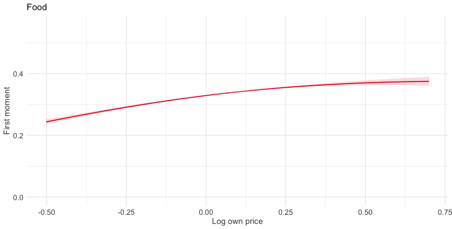
(a) Food: log own price

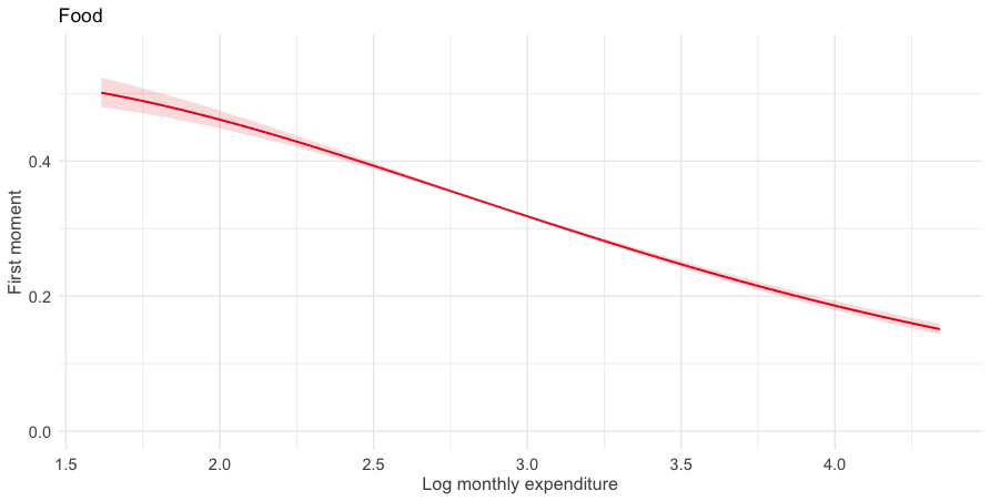
(b) Food: log household expenditure

Services

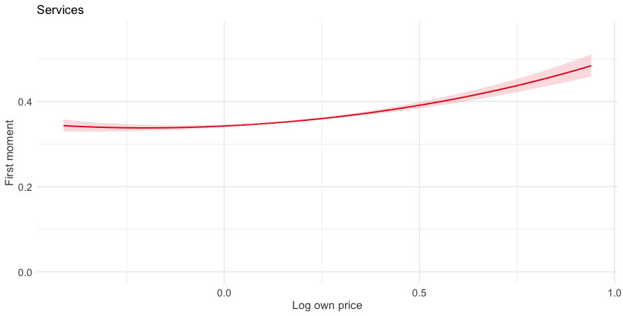
(c) Services: log own price

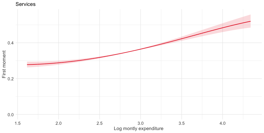
(d) Services: log household expenditure

Figure 7.1: First moments of budget shares

Food

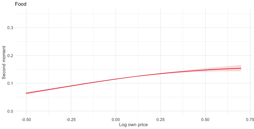
(a) Food: log own price

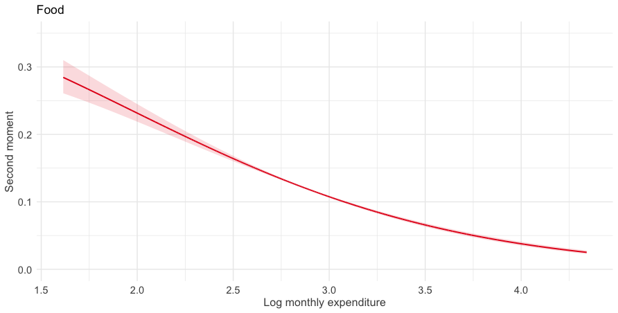
(b) Food: log household expenditure

Services

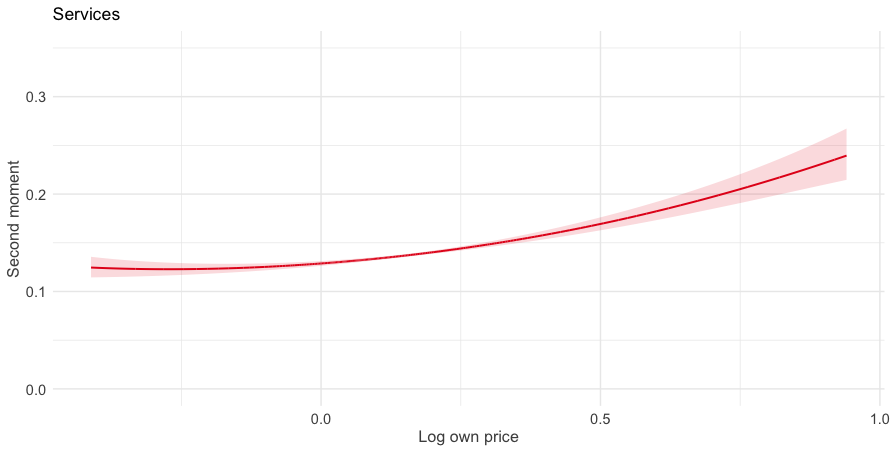
(c) Services: log own price

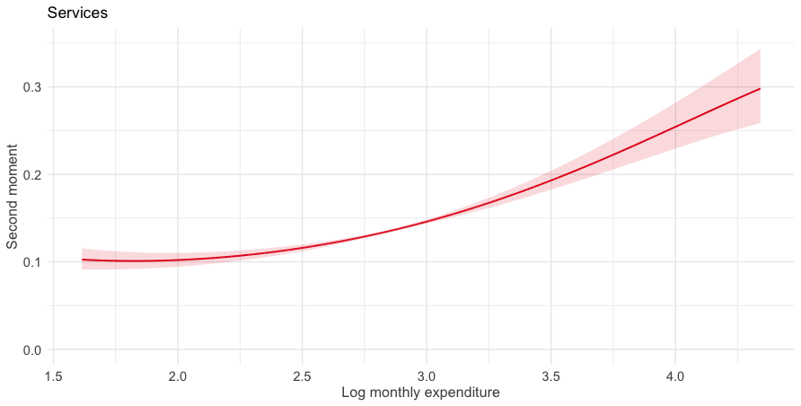
(d) Services: log household expenditure

Figure 7.2: Second moments of budget shares

Average welfare effects.

We first examine the average welfare impact of changes in the prices of food and services. In every of these two scenarios, the price of the other composite good is kept constant. To allow for meaningful interpersonal welfare comparisons, for every household we fix the vector of baseline prices to the sample median. Given the limited sampling variation in our moment estimates, all welfare effects are estimated with high statistical precision.

Our primary goal is to compare our robust welfare estimate with the approximation derived from the representative agent approach

$$\begin{split}\overline{CV}^{\omega}(p_{0},p_{1},y)&=\Delta pM_{1}(p_{0},y)+\frac{(\Delta p)^{2}}{2}\left(\frac{\partial}{\partial p}M_{1}(p_{0},y)+\frac{1}{2}\frac{\partial}{\partial y}(M_{1}(p_{0},y))^{2}\right),\end{split}$$

and the worst-case bounds, as detailed in Expression (5). To establish these bounds, we assume that every good $k$ is normal, such that $0\leq\frac{\partial q^{\omega}_{k}(p_{0},y)}{\partial y}\leq\frac{1}{p_{k0}}$ uniformly for every household $\omega$. The upper bound follows directly from the budget constraint and is attained when one additional unit of income is fully spent on good $k$.

Food

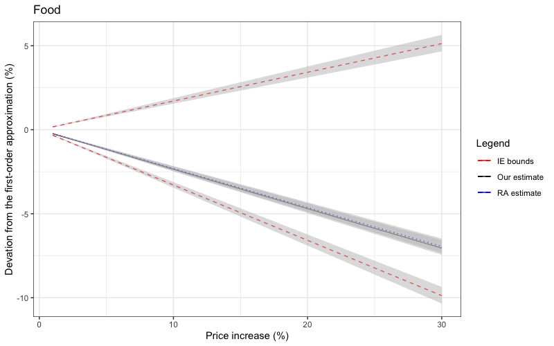
(a) Food: price increases

Services

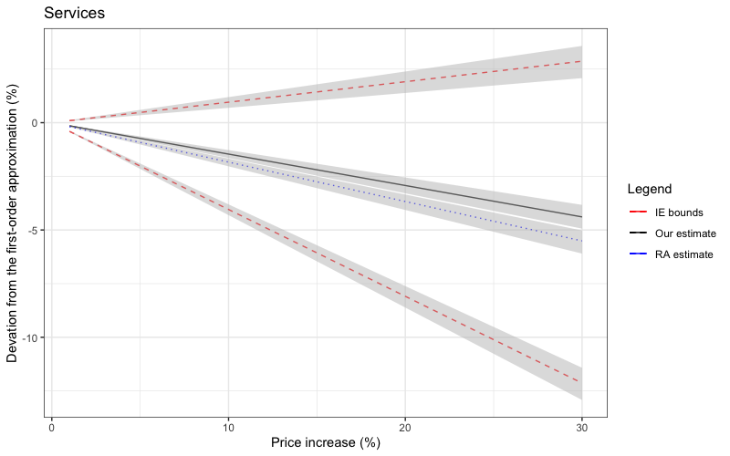
(b) Services: price increases

Figure 7.3: Robust local approximation to welfare — average

For price increases ranging from 0 to 30%, Figure 7.3 plots the deviation of our robust estimate, the representative-agent estimate, and the worst-case bounds with respect to the first-order approximation $\Delta pM_{1}(p_{0},y)$. Considering a 20% increase in food prices, we find that the first-order approximation (represented by the horizontal axis) overstates the true welfare impact by roughly 5%. Similarly, for a 20% price hike in services, the overestimation stands at approximately 2.5%. These results highlight the limitations of relying solely on the first-order approximation for assessing welfare impacts.

Interestingly, for both categories of composite goods, we see that the worst-case bounds encompass the first-order approximation, which assumes that individuals do not adjust their demand to prices. Given minimal knowledge on the magnitude of individuals’ income effects, these bounds are quite wide. In addition, we observe that for both categories the discrepancy between our estimate and that using the representative agent approach is relatively modest. This finding suggests that the bias introduced by the representative-agent approach, which is based on the assumption of homogeneous preferences among consumers, might be less significant in practice.

To assess heterogeneous welfare impacts across households, Table D.4 in the Appendix presents our robust estimate and the representative-agent estimate by decile of household expenditure. Our analysis reveals a noteworthy pattern: for food, we find that the relative deviation between our estimate and the first-order approach is larger for households with higher expenditure levels, while for services the reverse conclusion holds. This reflects that for household with lower levels of expenditure, it is hard to substitute away from food. On the other hand, the demand for services of households with high levels of expenditure is relative insensitive to price changes for these services. For services, our estimate and the representative-agent estimate differ the most for households with high expenditures. This indicates that for these households the covariance between demand and income effects is larger (and positive).

Table 7.1: Decomposition of the second-order contribution to the CV

		Food		Services
		Share (%)	90% CI	Share (%)	90% CI
$A_{1}$	RA/H	72.31	[69.33, 75.36]	150.90	[144.38, 159.45]
$A_{2}$	RA/NH	26.28	[23.36, 29.17]	-25.44	[-28.84, -21.80]
$A_{3}$	NRA/H	-4.66	[-4.94, -4.30]	-16.26	[-18.93, -14.32]
$A_{4}$	NRA/NH	6.06	[5.56, 6.66]	-9.20	[-13.71, -5.60]

(N)RA: (no) representative agent; (N)H: (non)-homothetic preferences

Finally, paralleling the approach in Corollary 1, we decompose the second-order contribution to welfare into components accounting for non-homothetic preferences and unobserved heterogeneity. The detailed breakdown of each component’s relative significance to the overall second-order contribution is presented in Table 7.1. A notable finding from this analysis is that for both categories of composite goods, incorporating behavioral responses, even within the constrained framework of a homothetic representative agent (i.e., $A_{1}$), forms the most substantial part of the second-order contribution. Interestingly, we find that the adjustment for non-homothetic preferences (i.e., $A_{1}+A_{2}$) plays a more crucial role than accounting for unobserved heterogeneity (i.e., $A_{1}+A_{3}$). This suggests that, in terms of bias reduction, nonparametric estimates that model a representative consumer may actually be more accurate compared to more complex models of homothetic demand that include preference heterogeneity. This conclusion is particularly relevant for essential goods like food, where the impact of non-homothetic preferences is more pronounced.

Variance of welfare effects.

We now turn to the spread of the welfare impacts throughout the population. As before, the price of the other composite good is kept constant in every of these two scenarios.

Our central aim is to derive a robust estimate for the variance in welfare impacts. Based on the approximation developed in Theorem 3, we can write

$$\begin{split}\text{Var}(CV^{\omega}(p_{0},p_{1},y))&=\mathbb{E}[CV^{\omega}(p_{0},p_{1},y)^{2}]-\mathbb{E}[CV^{\omega}(p_{0},p_{1},y)]^{2}\\ &\approx(\Delta p)^{2}\Bigg{[}\left(M_{2}(p_{0},y)+\frac{\Delta p}{2}\left[\frac{\partial M_{2}(p_{0},y)}{\partial p}+\frac{2}{3}\frac{\partial M_{3}(p_{0},y)}{\partial y}\right]\right)\\ &\quad-\left(M_{1}(p_{0},y)+\frac{\Delta p}{2}\left[\frac{\partial M_{1}(p_{0},y)}{\partial p}+\frac{1}{2}\frac{\partial M_{2}(p_{0},y)}{\partial y}\right]\right)^{2}\Bigg{]}.\end{split}$$

Unlike earlier, where the representative agent model served as a viable benchmark, it becomes inapplicable in the current context of estimating the variance of welfare impacts. The crux of the issue lies in the fundamental assumption of the representative agent model: the entire population is represented by a single, homogenized individual. This simplification leads to a degenerate distribution of welfare effects, rendering the variance of these effects undefined. As an alternative benchmark, we therefore consider the class of demand models that are additively separable in unobserved heterogeneity: i.e., $q^{\omega}(p_{0},y)=g(p_{0},y)+\varepsilon(\omega)$. For this class of models, it holds that

$$\begin{split}\text{Var}(CV_{AS}^{\omega}(p_{0},p_{1},y))&\approx(\Delta p)^{2}\Bigg{[}\left(M_{2}(p_{0},y)+\Delta p\left[M_{1}(p_{0},y)\frac{\partial M_{1}(p_{0},y)}{\partial p}+M_{2}(p_{0},y)\frac{\partial M_{1}(p_{0},y)}{\partial y}\right]\right)\\ &\quad-\left(M_{1}(p_{0},y)+\frac{\Delta p}{2}\left[\frac{\partial M_{1}(p_{0},y)}{\partial p}+M_{1}(p_{0},y)\frac{\partial M_{1}(p_{0},y)}{\partial y}\right]\right)^{2}\Bigg{]}.\end{split}$$

Juxtaposing these two estimates allows us to assess how restrictive this separability assumption is for estimating the variance of welfare impacts. The importance of this comparison stems from the fact that many parametric demand systems, widely used in welfare analysis, are built on the foundation of additive separability in unobservables. While this assumption simplifies the modeling process, it may also introduce constraints that can skew the understanding of welfare impacts.

For price increases ranging from 0 to 30%, Figure 7.4 plots the relative discrepancies of these variances with respect to the variance based on the first-order approximation. For food, we find that our robust estimate significantly undercuts that of the first-order approximation (again represented by the horizontal axis). This deviation is primarily attributed to the negative correlation between individuals’ behavioral responses and their demand, which effectively reduces the overall variance. Furthermore, we also find that the additively-separable estimate significantly overstates the variance of welfare effects. For example for a 20% increase in food prices, the gap in both estimates amounts to more than 13%p. Similarly for services, we find that the additively-separable estimate is considerably larger than our robust estimate, although to a lesser extent. In this case our robust estimate is statistically indistinguishable form the variance based on the first-order approximation. Taken together, our results suggest that both estimates based on first-order approximations and estimates based on the assumption of additive separability might significantly overstate the spread of welfare impacts in the population.

Food

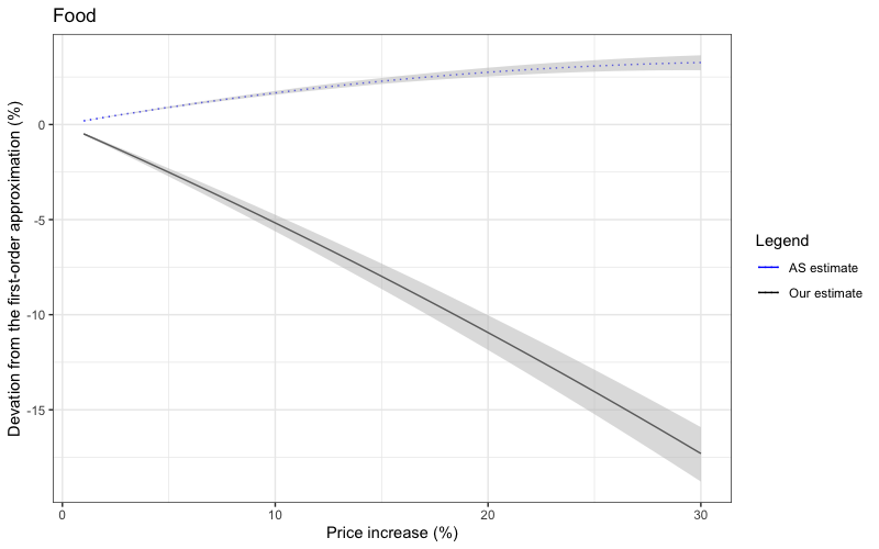
(a) Food: price increases

Services

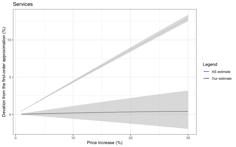
(b) Services: price increases

Figure 7.4: Robust local approximation to welfare — variance

8 Concluding remarks

In this paper, we introduce novel methods to approximate moments of compensated demand through moments of uncompensated demand. To do so, we show that the moments of demand contain information about the distribution of individuals’ income effects. We use this information to conduct more accurate counterfactual exercises in applied welfare analysis. We also demonstrate that better approximations cannot be found using cross-sections.

Going forward, there is room for future work in at least four directions. Firstly, it would be interesting to understand what additional power short panels on consumers would give to estimate the above counterfactuals; first steps in this direction has been made by Crawford (2019) and Cooprider, Hoderlein, and Alexander (2022). Secondly, another promising avenue of research is to extend our approach to general equilibrium models to improve, for example, the measurement of the welfare gains (and losses) from trade (Baqaee and Burstein, 2022). Thirdly, it would be fruitful to have a better understanding of welfare analysis in models that deviate from rationality. Recent contribution in this regard has been made by Apesteguia and Ballester (2015) and Aguiar and Serrano (2017). Finally, more work should be done on efficient estimation in settings with many goods. Recent advances in high-dimensional statistics can be used to overcome the curse of dimensionality, a problem which is further complicated by the potential endogeneity of budget sets. In this regard, extending the results by Chernozhukov, Hausman, and Newey (2019) seems to be a fruitful avenue for future research.

Appendix A Regularity conditions

Every individual’s demand function $\mathbf{q}^{\omega}$ needs to be infinitely differentiable in $\mathbf{p},y$ at all $\mathbf{p},y\in\mathcal{P}\times\mathcal{Y}$. This is ensured by the following condition.

Assumption 1.

Every individual’s preferences are continuous, strictly convex, and locally nonsatiated. The associated utility functions $u^{\omega}$ are infinitely differentiable everywhere.

The following condition ensures that the dominated convergence theorem holds. This allows us to interchange limits and integrals.

Assumption 2.

There exists a function $g:\Omega\rightarrow\mathbb{R}$ such that for all $\mathbf{p},y\in\mathcal{P}\times\mathcal{Y}$ and $n,m\in\mathbb{N}$ it holds that $\|\text{vec}(D_{p^{n},y^{B}}\mathbf{q}^{\omega}(\mathbf{p},y))\|\leq g(\omega)$ with $\int g(\omega)dF(\omega)<\infty$.

Finally, we require that all moments exist and are finite.

Assumption 3.

For all $n\in\mathbb{N}$, it holds that

$$\mathbb{E}\left[|\mathbf{T}^{\omega}_{n}(\mathbf{p},y)|\right]<\infty.$$

Appendix B Proofs omitted in the main text

B.1 Proof of Theorem 1

Using a first-order Taylor approximation around $t=0$, we have that

$$\begin{split}h^{\omega}(p_{0}+t\Delta p,v_{0}^{\omega})^{n}&=h^{\omega}(p_{0},v_{0}^{\omega})^{n}+\left(h^{\omega}(p_{0},v_{0}^{\omega})^{n-1}\frac{\partial}{\partial p}h^{\omega}(p_{0},v_{0}^{\omega})\right)t\Delta p+\eta\\ &=q^{\omega}(p_{0},y)^{n}+\left(q^{\omega}(p_{0},y)^{n-1}\left(\frac{\partial}{\partial p}q^{\omega}(p_{0},y)+q^{\omega}(p_{0},y)\frac{\partial}{\partial y}q^{\omega}(p_{0},y)\right)\right)t\Delta p+O((\Delta p)^{2}).\\ \end{split}$$

Taking expectations at both sides gives

$$\mathbb{E}[h^{\omega}(p_{0}+t\Delta p,v_{0}^{\omega})^{n}]=M_{n}(p_{0},y)+\left(\frac{1}{n}\frac{\partial}{\partial p}M_{n}(p_{0},y)+\frac{1}{n+1}\frac{\partial}{\partial y}M_{n+1}(p_{0},y)\right)t\Delta p+O((\Delta p)^{2}).$$

B.2 Proof of Corollary 1

Similarly to previous section, we can approximate

$$\begin{split}w_{h}^{\omega}(p_{0}+t\Delta p,v_{0}^{\omega})^{n}&\approx w_{h}^{\omega}(p_{0},v_{0}^{\omega})^{n}+\left(w_{h}^{\omega}(p_{0},v_{0}^{\omega})^{n-1}\frac{\partial}{\partial p}w_{h}^{\omega}(p_{0},v_{0}^{\omega})\right)t\Delta p\\ &=w^{\omega}(p_{0},y)^{n}+\frac{1}{y}\left(w^{\omega}(p_{0},y)^{n-1}\left(q^{\omega}(p_{0},y)+p_{0}\frac{\partial}{\partial p}h^{\omega}(p_{0},v_{0}^{\omega})\right)\right)t\Delta p\\ &=w^{\omega}(p_{0},y)^{n}+\frac{1}{y}\left(w^{\omega}(p_{0},y)^{n-1}\left(q^{\omega}(p_{0},y)+p_{0}\left(\frac{\partial q(p_{0},y)}{\partial p}+q(p_{0},y)\frac{\partial q(p_{0},y)}{\partial y}\right)\right)\right)t\Delta p.\end{split}$$

Differentiating the identity for the budget share with respect to price and income and rearranging gives

$$\begin{split}\frac{p_{0}}{y}\frac{\partial}{\partial p}q^{\omega}(p_{0},y)&=\frac{\partial}{\partial p}w^{\omega}(p_{0},y)-\frac{1}{y}q^{\omega}(p_{0},y),\\ \frac{p_{0}}{y}\frac{\partial}{\partial y}q^{\omega}(p_{0},y)&=\frac{\partial}{\partial y}w^{\omega}(p_{0},y)+\frac{p_{0}}{y^{2}}q^{\omega}(p_{0},y).\end{split}$$

These expressions, together with repeated application of the identity for the budget share yields

$$\begin{split}w_{h}^{\omega}(p_{0}+t\Delta p,v_{0}^{\omega})^{n}&\approx w^{\omega}(p_{0},y)^{n}+\left(\frac{1}{n}\frac{\partial}{\partial p}w^{\omega}(p_{0},y)^{n}+\frac{1}{n+1}\frac{y}{p_{0}}\frac{\partial}{\partial y}w^{\omega}(p_{0},y)^{n+1}+\frac{1}{p_{0}}w^{\omega}(p_{0},y)^{n+1}\right)t\Delta p\\ &=w^{\omega}(p_{0},y)^{n}+\left(\frac{1}{n}\frac{\partial}{\partial\log p}w^{\omega}(p_{0},y)^{n}+\frac{1}{n+1}\frac{\partial}{\partial\log y}w^{\omega}(p_{0},y)^{n+1}+w^{\omega}(p_{0},y)^{n+1}\right)t\frac{\Delta p}{p_{0}}.\end{split}$$

Taking expectations at both sides gives the desired result:

$$\begin{split}\mathbb{E}[w_{h}^{\omega}(p_{0}+t\Delta p,v_{0}^{\omega})^{n}]&\approx W_{n}(p_{0},y)+\left(\frac{1}{n}\frac{\partial}{\partial\log p}W_{n}(p_{0},y)+\frac{1}{n+1}\frac{\partial}{\partial\log y}W_{n+1}(p_{0},y)+W_{n+1}(p_{0},y)\right)t\frac{\Delta p}{p_{0}}.\end{split}$$

B.3 Proof for Theorem 3

We have that the $n$th moment of the CV is equal to

$$\begin{split}\mathbb{E}[CV^{\omega}(p_{0},p_{1},y)^{n}]&=(\Delta p)^{n}\mathbb{E}\left[\left(\int_{0}^{1}h^{\omega}(p_{0}+t\Delta p,v^{\omega}_{0})dt\right)^{n}\right]\\ &=(\Delta p)^{n}\mathbb{E}\left[\int_{0}^{1}\dots\int_{0}^{1}\prod_{i=1}^{n}h^{\omega}(p_{0}+t_{i}\Delta p,v^{\omega}_{0})dt_{1}\dots dt_{n}\right].\\ \end{split}$$

Using a first-order Taylor approximation around $t_{i}=0$ for all $i$, we have that

$$\begin{split}\prod_{i=1}^{n}h^{\omega}(p_{0}+t_{i}\Delta p,v_{0}^{\omega})&=h^{\omega}(p_{0},v_{0}^{\omega})^{n}+\Delta p\left(\sum_{i=1}^{n}t_{i}\right)h^{\omega}(p_{0},v_{0}^{\omega})^{n-1}\frac{\partial}{\partial p}h^{\omega}(p_{0},v_{0}^{\omega})+O((\Delta p)^{2})\\ &=q^{\omega}(p_{0},y)^{n}+\Delta p\left(\sum_{i=1}^{n}t_{i}\right)q^{\omega}(p_{0},y)^{n-1}\frac{\partial}{\partial p}h^{\omega}(p_{0},v_{0}^{\omega})+O((\Delta p)^{2}).\\ \end{split}$$

Putting things together, we have that

$$\begin{split}\mathbb{E}[CV^{\omega}(p_{0},p_{1},y)^{n}]&=(\Delta p)^{n}\mathbb{E}\Bigg{[}\int_{0}^{1}\dots\int_{0}^{1}q^{\omega}(p_{0},y)^{n}+\Delta p\left(\sum_{i=1}^{n}t_{i}\right)q^{\omega}(p_{0},y)^{n-1}\frac{\partial}{\partial p}h^{\omega}(p_{0},v_{0}^{\omega})\\ &\quad+O((\Delta p)^{2})dt_{1}\dots dt_{n}\Bigg{]}\\ &=(\Delta p)^{n}\left[M_{n}(p_{0},y)+\frac{\Delta p}{2}\left(\frac{\partial}{\partial p}M_{n}(p_{0},y)+\frac{n}{n+1}\frac{\partial}{\partial y}M_{n+1}(p_{0},y)\right)+O((\Delta p)^{2})\right],\end{split}$$

where the last equality follows from the Slutsky equation.

Appendix C Additional results

C.1 Results for welfare in the many-goods case

Moments of demand.

In the many-good case, one can express the $n$th moment of demand by means of the symmetric $n$ tensor $\mathbf{T}^{\omega}_{n}(\mathbf{p},y)$ for which the element $t^{\omega}_{i_{1},i_{2},\dots i_{n}}(\mathbf{p},y)=q^{\omega}_{i_{1}}(\mathbf{p},y)q^{\omega}_{i_{2}}(\mathbf{p},y)\dots q^{\omega}_{i_{n}}(\mathbf{p},y)$ with $i_{1},i_{2},\dots,i_{n}\in\{1,2,\dots,k\}$. We define the generalized tensor form of $\mathbf{T}^{\omega}_{n}(\mathbf{p},y)$ with respect a vector $\mathbf{v}\in\mathbb{R}^{k}$ as the multilinear function

$$\begin{split}\mathbf{v}(**)\mathbf{T}^{\omega}_{n}(\mathbf{p},y)&=\mathbf{T}^{\omega}_{n}(\mathbf{p},y)(\underbrace{\mathbf{v}\times\mathbf{v}\dots\times\mathbf{v}}_{\text{$n$ times}})\\ &=\sum_{i_{1},i_{2},\dots,i_{n}=1}^{k}t^{\omega}_{i_{1},i_{2},\dots,i_{n}}(\mathbf{p},y)v_{i_{1}}v_{i_{2}}\dots v_{i_{n}}.\end{split}$$

Again, by integrating out unobserved preference heterogeneity, we can express the $n$th (non-central) moment of demand as

$$\begin{split}\mathbf{M}_{n}(\mathbf{p},y)&=\mathbb{E}\left[\mathbf{T}^{\omega}_{n}(\mathbf{p},y)\right]\\ &=\int\mathbf{T}^{\omega}_{n}(\mathbf{p},y)dF(\omega\mid\mathbf{p},y).\\ \end{split}$$ (17)

We define a moment sequence as the (possibly infinite) sequence $\{\mathbf{M}_{i}(\mathbf{p},y)\}_{i=1}^{n}$ of the first $n$ moments of demand.

Welfare estimation.

We now analyze the distribution of the CV in the case where there are more than two goods. This requires what we refer to as a symmetrization procedure: i.e., to obtain an estimate of the average substitution effect, we need to impose Slutsky symmetry.

Lemma 1.

Analogously with the two-goods case, the following holds for three or more goods,

$$\mathbb{E}\left[\frac{\partial}{\partial p}\mathbf{h}^{\omega}(\mathbf{p},u)\right]=\frac{1}{2}\left(\frac{\partial}{\partial p}\mathbf{M}_{1}(\mathbf{p},y)+\frac{\partial}{\partial p}\mathbf{M}_{1}(\mathbf{p},y)^{\intercal}+\frac{\partial}{\partial y}\mathbf{M}_{2}(\mathbf{p},y)\right).$$

Proof.

Using the definition of the conditional moments in Expression (17), we know that

$$\begin{split}\frac{\partial}{\partial y}\mathbf{M}_{2}(\mathbf{p},y)&=\frac{\partial}{\partial y}\left(\int\mathbf{q}^{\omega}(\mathbf{p},y)(\mathbf{q}^{\omega}(\mathbf{p},y))^{\intercal}dF(\omega)\right).\end{split}$$

Interchanging the derivative and integral operators gives us

$$\begin{split}\frac{\partial}{\partial y}\mathbf{M}_{2}(\mathbf{p},y)&=\int\frac{\partial}{\partial y}(\mathbf{q}^{\omega}(\mathbf{p},y)(\mathbf{q}^{\omega}(\mathbf{p},y))^{\intercal})dF(\omega)\\ &=\int_{\omega}\left[\frac{\partial}{\partial y}\mathbf{q}^{\omega}(\mathbf{p},y)(\mathbf{q}^{\omega}(\mathbf{p},y))^{\intercal}+\mathbf{q}^{\omega}(\mathbf{p},y)(\frac{\partial}{\partial y}\mathbf{q}^{\omega}(\mathbf{p},y))^{\intercal}\right]dF(\omega).\end{split}$$

From the Slutsky equation (7), we have that

$$\frac{\partial}{\partial p}\mathbf{h}^{\omega}(\mathbf{p},u)=\frac{\partial}{\partial p}\mathbf{q}^{\omega}(\mathbf{p},y)+\frac{\partial}{\partial y}\mathbf{q}^{\omega}(\mathbf{p},y)(\mathbf{q}^{\omega}(\mathbf{p},y))^{\intercal},$$

which is symmetric due to Slutsky symmetry. Adding this equation to its transpose fetches us

$$2\frac{\partial}{\partial p}\mathbf{h}^{\omega}(\mathbf{p},u)=\frac{\partial}{\partial p}\mathbf{q}^{\omega}(\mathbf{p},y)+\left(\frac{\partial}{\partial p}\mathbf{q}^{\omega}(\mathbf{p},y)\right)^{\intercal}+\frac{\partial}{\partial y}\mathbf{q}^{\omega}(\mathbf{p},y)(\mathbf{q}^{\omega}(\mathbf{p},y))^{\intercal}+\mathbf{q}^{\omega}(\mathbf{p},y)\left(\frac{\partial}{\partial y}\mathbf{q}^{\omega}(\mathbf{p},y)\right)^{\intercal},$$

such that

$$\begin{split}\mathbb{E}\left[\frac{\partial}{\partial p}\mathbf{h}^{\omega}(\mathbf{p},u)\right]&=\frac{1}{2}\left[\frac{\partial}{\partial p}\mathbf{M}_{1}(\mathbf{p},y)+\left(\frac{\partial}{\partial p}\mathbf{M}_{1}(\mathbf{p},y)\right)^{\intercal}+\frac{\partial}{\partial y}\mathbf{M}_{2}(\mathbf{p},y)\right].\end{split}$$

∎

Using this symmetrization procedure, we can obtain second-order approximations for all moments of the compensating variation. The following theorem makes this formal.

Theorem 6.

In the many-good case, the second-order approximation of the $n$th moment of the compensating variation depends only on the $n$th and $(n+1)$th moment of demand. Formally, we have that

$$\mathbb{E}[CV^{\omega}(\mathbf{p}_{0},\mathbf{p}_{1},y)^{n}]=\mathbf{p}(**)\left\{\frac{1}{n}\left[\sum(\text{symmetrized moment derivative})\right]+\frac{n}{n+1}\frac{\partial}{\partial y}\mathbf{M}_{n+1}\right\}.$$

Proof.

The proof is similar to that of Theorem 3. With more than two goods, demand is a vector, which fetches us the formula

$$\mathbb{E}[CV^{\omega}(\mathbf{p}_{0},\mathbf{p}_{1},y)^{n}]=\mathbb{E}\left[\left(\int_{0}^{1}\Delta\mathbf{p}\cdot\mathbf{h}^{\omega}(\mathbf{p}_{0}+t\Delta\mathbf{p},v^{\omega}_{0})dt\right)^{n}\right].$$

Again, using the first-order expansion of compensated demand around $t=1$, we have that

$$\begin{split}\mathbb{E}[CV^{\omega}(\mathbf{p}_{0},\mathbf{p}_{1},y)^{n}]&\approx\left[\Delta\mathbf{p}\cdot\mathbf{h}^{\omega}(\mathbf{p}_{0},v^{\omega}_{0})\right]^{n}\\ &\quad+\sum_{1=1}^{n}(\Delta\mathbf{p}\cdot\mathbf{h}^{\omega}(\mathbf{p}_{0},v^{\omega}_{0}))^{i}\left[\Delta\mathbf{p}\frac{\partial}{\partial p}\mathbf{h}^{\omega}(\mathbf{p}_{0},v^{\omega}_{0})(\Delta\mathbf{p})^{\intercal}\right](\Delta\mathbf{p}\cdot\mathbf{h}^{\omega}(\mathbf{p}_{0},v^{\omega}_{0}))^{n-i-1}.\end{split}$$

Plugging in the Slutsky equation in the second term gives

$$\sum_{1=1}^{n}(\Delta\mathbf{p}\cdot\mathbf{q}^{\omega}(\mathbf{p}_{0},y))^{i}\left[\Delta\mathbf{p}(\frac{\partial}{\partial p}\mathbf{q}^{\omega}(\mathbf{p}_{0},y)+\frac{\partial}{\partial y}\mathbf{q}^{\omega}(\mathbf{p}_{0},y))(\Delta\mathbf{p})^{\intercal}\right](\Delta\mathbf{p}\cdot\mathbf{q}^{\omega}(\mathbf{p}_{0},y))^{n-i-1},$$

or after expanding,

$$\begin{split}&\sum_{1=1}^{n}(\Delta\mathbf{p}\cdot\mathbf{q}^{\omega}(\mathbf{p}_{0},y))^{i}(\Delta\mathbf{p}\frac{\partial}{\partial p}\mathbf{q}^{\omega}(\mathbf{p}_{0},y)(\Delta\mathbf{p})^{\intercal})(\Delta\mathbf{p}\cdot\mathbf{q}^{\omega}(\mathbf{p}_{0},y))^{n-i-1}\\ &+\sum_{1=1}^{n}(\Delta\mathbf{p}\cdot\mathbf{q}^{\omega}(\mathbf{p}_{0},y))^{i}(\frac{\partial}{\partial y}\mathbf{q}^{\omega}(\mathbf{p}_{0},y)(\Delta\mathbf{p})^{\intercal})(\Delta\mathbf{p}\cdot\mathbf{q}^{\omega}(\mathbf{p}_{0},y))^{n-i-1}.\end{split}$$

The analyst, however, observes

$$\frac{\partial}{\partial y}\mathbf{M}_{n+1}=\sum_{i=1}^{n}\mathbb{E}\left[\left(\bigotimes_{k=1}^{i}\mathbf{q}^{\omega}(\mathbf{p},y)\right)\bigotimes\frac{\partial}{\partial y}\left(\bigotimes_{k=1}^{n-i-1}\mathbf{q}^{\omega}(\mathbf{p},y)\right)\right].$$

As with the variance, one can be written in terms of the other by means of symmetrization, giving us

$$\Delta\mathbf{p}(**)\frac{1}{n}\sum_{k=1}^{n}\frac{\partial}{\partial p}\mathbf{M}_{n}(\mathbf{p},y)^{\intercal_{k}}+\frac{n}{n+1}\frac{\partial}{\partial y}(\mathbf{M}_{n+1})(\mathbf{p},y),$$

where (**) is the generalized tensor form and $\frac{1}{n}\sum_{k=1}^{n}\frac{\partial}{\partial p}\mathbf{M}_{n}(b)^{\intercal_{k}}$ is the symmetrized version of the tensor.

Notice that for higher-order tensors, in order to symmetrize them, we need to carry out a cyclic transformation which sends element $a_{i_{1},i_{2},\dots,i_{k+1}}\to a_{i_{k+1},i_{1},\dots,i_{k}}$. There are $k$ such transformations, hence they sum upto $k$.

∎

Remark 1.

When the prices of all goods change, the second-order approximation for the average compensating variation requires estimating the entire variance-covariance matrix, which might be burdensome. However, it is possible to bound the off-diagonal elements of this matrix from the marginal variances. In particular, one can impose the following restrictions:

$$\begin{split}\left[\mathbf{M}^{2}(\mathbf{p},y)\right]_{ij}&=\left[\mathbf{M}^{2}(\mathbf{p},y)\right]_{ji},\\ \mathbf{p}\cdot\frac{\partial}{\partial y}\mathbf{M}_{2}(\mathbf{p},y)&=\frac{\partial}{\partial y}\mathbf{M}_{2}(\mathbf{p},y)\cdot\mathbf{p}=0,\\ \left[\mathbf{M}^{2}(\mathbf{p},y)\right]_{ij}&\leq\sqrt{[\mathbf{M}^{2}(\mathbf{p},y)_{ii}\mathbf{M}^{2}(\mathbf{p},y)]_{jj}}.\end{split}$$

The first restriction follows the symmetry of the variance-covariance matrix, the second is the budget constraint, and the third is due to the Cauchy-Schwarz inequality. Note that the Cauchy-Schwarz inequality ensures that the off-diagonal elements have bounded support, even if we would only observe the diagonal elements.

C.2 Nonidentification of the third-order approximation to welfare

Lemma 2.

Then $\{\mathbb{E}[q^{\omega}(\mathbf{p},y)(\frac{\partial}{\partial y}q^{\omega}(\mathbf{p},y))^{n}])\}_{n=2}^{\infty}$ is not nonparametrically identified from cross-sectional data.

Proof.

We show nonidentification of $\{\mathbb{E}[q^{\omega}(\mathbf{p},y)(\frac{\partial}{\partial y}q^{\omega}(\mathbf{p},y))^{n}])\}_{n=2}^{\infty}$ by means of a counterexample. Suppose individual demand is linear in price and income

$$q^{\omega}(\mathbf{p},y)=\omega_{1}-p+\omega_{2}y,$$

and let $\omega_{1}\sim U(0,1)$, and $\Pr\left[\omega_{2}=1/3\right]=\Pr\left[\omega_{2}=2/3\right]=1/2$. Hausman and Newey (2016) show that for $y<3$, an observationally equivalent specification is the quantile demand

$$\widetilde{q}^{\widetilde{\omega}}(\mathbf{p},y)=\begin{cases}-p+\mathbb{I}[y<6\widetilde{\omega}](y/2+\widetilde{\omega})+\mathbb{I}[y\geq 6\widetilde{\omega}](y/3+2\widetilde{\omega}),&\widetilde{\omega}\leq 1/2,\\ -p+\mathbb{I}[y<6(1-\widetilde{\omega})](y/2+\widetilde{\omega})+\mathbb{I}[y\geq 6(1-\widetilde{\omega})](2y/3+2\widetilde{\omega}-1),&\widetilde{\omega}>1/2,\\ \end{cases}$$

where $\widetilde{\omega}\sim U(0,1)$.

For a budget set $(p,y)=(1,2)$, elementary calculations show that

$$\begin{split}\mathbb{E}\left[q^{\omega}(\mathbf{p},y)\left(\frac{\partial}{\partial y}q^{\omega}(\mathbf{p},y)\right)^{n}\right]&=\mathbb{E}[(\omega_{1}-p+\omega_{2}y)\omega_{2}^{n}\mid p=1,y=2]\\ &=(\mathbb{E}\left[\omega_{1}\right]-1)\mathbb{E}\left[\omega_{2}^{n}\right]+2\mathbb{E}\left[\omega_{3}^{n}\right]\\ &=-1/4[(1/3)^{n}+(2/3)^{n}]+[(1/3)^{n+1}+(2/3)^{n+1}]\\ &=1/12(1/3)^{n}+5/12(2/3)^{n}\end{split}$$ (18)

holds for the original demand specification. However, after differentiating the quantile demand with respect to income, we obtain

$$\widetilde{q}^{\widetilde{\omega}}(\mathbf{p},y)\left(\frac{\partial}{\partial y}\widetilde{q}^{\widetilde{\omega}}(\mathbf{p},y)\right)^{n}\mid_{p=1,y=2}=\begin{cases}\begin{split}\mathbb{I}[1/3<\widetilde{\omega}]\widetilde{\omega}(1/2)^{n}+\mathbb{I}[1/3\geq\widetilde{\omega}](-1/3+2\widetilde{\omega})(1/3)^{n}\end{split},&\widetilde{\omega}\leq 1/2,\\ \begin{split}\mathbb{I}[2/3>\widetilde{\omega}]\widetilde{\omega}(1/2)^{n}+\mathbb{I}[2/3\leq\widetilde{\omega}](-2/3+2\widetilde{\omega})(2/3)^{n}\end{split},&\widetilde{\omega}>1/2,\\ \end{cases}$$

such that

$$\begin{split}\mathbb{E}\left[\widetilde{q}^{\widetilde{\omega}}(\mathbf{p},y)\left(\frac{\partial}{\partial y}\widetilde{q}^{\widetilde{\omega}}(\mathbf{p},y)\right)^{n}\right]&=(1/3)^{n}\int_{0}^{1/3}(-1/3+2\widetilde{\omega})+(1/2)^{n}\int_{1/3}^{1/2}\widetilde{\omega}\\ &\quad+(1/2)^{n}\int_{1/2}^{2/3}\widetilde{\omega}+(2/3)^{n}\int_{2/3}^{1}(-2/3+2\widetilde{\omega})\\ &=1/6(1/2)^{n}+1/3(2/3)^{n}.\end{split}$$ (19)

Expressions (18) and (19) are only equal for $n=1$. Since two observationally equivalent models generate different results for $n\geq 2$, $\{\mathbb{E}[q^{\omega}(\mathbf{p},y)(\frac{\partial}{\partial y}q^{\omega}(\mathbf{p},y))^{n}])\}_{n=2}^{\infty}$ are not nonparametrically identified. ∎

C.3 Income effect bounds and the Hausman and Newey approach

This section discusses the reduction in bounds that our approach offers to the Hausman and Newey (2016) approach. If income effects are bounded, i.e., $A\leq IE^{\omega}\leq B,\forall\omega\in\Omega$, it holds that

$$\Delta p\int_{0}^{1}q^{\omega}(p(t),y)e^{A\Delta pt}dt\leq\mathbb{E}[CV]\leq\Delta p\int_{0}^{1}q^{\omega}(p(t),y)e^{B\Delta pt}dt.$$

We can rewrite the left-hand side as

$$\begin{split}\Delta p\int_{0}^{1}q^{\omega}(p(t),y)e^{A\Delta pt}dt&=\Delta p\int_{0}^{1}\left[q^{\omega}(p(t),y)\right]\left[1+A\Delta pt+O(\Delta p)^{2}\right]dt\\ &=\Delta p\int_{0}^{1}\left[q^{\omega}(p(t),y)dt\right]+(\Delta p)^{2}A\int_{0}^{1}\left[q^{\omega}(p(t),y)tdt\right]+O(\Delta p)^{3}.\end{split}$$

The second term can be further simplified by carrying out integration by parts:

$$\int_{0}^{1}\left[q^{\omega}(p(t),y)tdt\right]=\int_{0}^{1}\left[q^{\omega}(p(t),y)dt\right]-\bigintsss_{0}^{1}\left[\int_{0}^{s}\left\{q^{\omega}(p(s),y)ds\right\}\right]dt.$$

This implies that the range of the Hausman and Newey (2016) bounds amounts to

$$(A-B)(\Delta p)^{2}\left[\int_{0}^{1}\left[q^{\omega}(p(t),y)dt\right]-\bigintsss_{0}^{1}\left[\int_{0}^{s}\left\{q^{\omega}(p(s),y)ds\right\}\right]dt\right]+O(\Delta p)^{3}.$$

We know turn to the maximum plausible theoretical deviation. Let

$$CV(X)=\Delta p\int_{0}^{1}\left[q^{\omega}(p(t),y)dt\right]+(\Delta p)^{2}X\int_{0}^{1}\left[q^{\omega}(p(t),y)tdt\right].$$

Set $X=B=0$, such that

$$\begin{split}\frac{CV(A)-CV(B)}{CV(B)}=A\Delta p\times\left[1-\frac{\bigintsss_{0}^{1}\left[\int_{0}^{s}\left\{q^{\omega}(p(s),y)ds\right\}\right]dt}{\int_{0}^{1}\left[q^{\omega}(p(t),y)dt\right]}\right],\end{split}$$

which is observable and close to half when price effects are small. When $A=\frac{1}{p}$, we have

$$\frac{CV(A)-CV(B)}{CV(B)}=\frac{\Delta p}{p}\left[1-\frac{\bigintsss_{0}^{1}\left[\int_{0}^{s}\left\{q^{\omega}(p(s),y)ds\right\}\right]dt}{\int_{0}^{1}\left[q^{\omega}(p(t),y)dt\right]}\right]\approx\frac{1}{2}\frac{\Delta p}{p}.$$

This reflects the bounds in the first-order approach via the Hausman and Newey (2016) approach and the reduction of the uncertainty we offer. For example, if prices increase by $15\%$ we reduce the uncertainty in the estimates by around $7.5\%$.

C.4 A Hicksian representative agent

Lemma 3 (Integrability of Expenditure Functions).

Let $f(p)$ be a (smooth) function from prices to the real numbers with two properties: the Hessian matrix of $f$ is negative semidefinite, and all price derivatives are positive, then f (locally) corresponds to the expenditure function of some (unique) utility.

Proof.

Existence follows from the integrability conditions in Border (2003) and uniqueness follws as smoothness guarantees the lipshitz property and then we can appeal to Mas-Colell (1977). ∎

Corollary 1 (Existence and Uniqueness).

There exists a utility function $U^{*}$ such that $U^{*}$ generates $e^{total}(p,u^{*})$.

Proof.

We need to check that

$$\frac{e^{total}(p,u^{*})}{dp_{i}}>0$$

and

$$\mathcal{H}_{e^{total}}\quad\text{is Negative Semidefinite}.$$

As both derivaties and Hessians are additive, the properties of the individual expenditure functions are inherited by the sum hence both these properties hold. ∎

The hicksian RA generically exists because the only restriction demand theory places on expenditure functions is that they are increasing and convex in prices. Both of these are preserved under addition. This is starkly different from the Usual or Marshallian Representative agent.

Notice that even if a Marshallian RA exists, it may not correspond to a Hicksian RA. We show this in the next example.

Example 1.

Take an economy with two Cobb-Douglas agents and two goods.

$$q^{1}(p_{1},p_{2},y) =\left(\frac{\alpha y}{p_{1}},\frac{(1-\alpha)y}{p_{2}}\right)$$

$$q^{2}(p_{1},p_{2},y) =\left(\frac{(1-\alpha)y}{p_{1}},\frac{\alpha y}{p_{2}}\right),$$

The Marshiallian RA has preferences resulting from the aggregate demand function

$$q^{RA}(p_{1},p_{2},y)=\left(\frac{y}{2p_{1}},\frac{y}{2p_{2}}\right)$$

or

$$e^{RA}(p_{1},p_{2},u^{*})=u^{*}\left(p_{1}^{1/2},p_{2}^{1/2}\right),$$

whereas the Hicksian RA would have

$$e^{total}(p_{1},p_{2},u^{*})=\frac{u^{*}}{2}\left[p_{1}^{\alpha},p_{2}^{1-\alpha}+p_{1}^{1-\alpha}p_{2}^{\alpha}\right].$$

This shows an interesting link: the Marshallian RA takes the geometric mean of expenditure functions, whereas the Hicksian takes the arithmetic mean. By the AM-GM inequality it holds that

$$e^{RA}(p_{1},p_{2},u^{*})\leq e^{total}(p_{1},p_{2},u^{*}),$$

with equality only in the case where there is no heterogeneity.

Appendix D Empirical application

D.1 Descriptive statistics

Table LABEL:tab:descriptives provides descriptive statistics for our estimation sample. Both prices for food and services and household expenditure are normalized with respect to the price of non-durables.

As noted in the main text, there was substantial variation in budget shares and relative prices for the three composite goods in the period under consideration. Overall, the budget share of food fell over time, whereas that of services rose; the price of services increased relative to that of food and non-durables.

Table D.1: Descriptive statistics of the estimation sample

Variable	Year	${n}$	Min	${q_{1}}$	${\bar{x}}$	${q_{3}}$	Max
$w_{food}$	75	1,507	0.06	0.30	0.37	0.43	0.75
	76	1,280	0.01	0.30	0.36	0.43	0.69
	77	1,384	0.01	0.30	0.37	0.43	0.76
	78	1,258	0.05	0.30	0.36	0.42	0.71
	79	1,228	0.05	0.29	0.35	0.42	0.70
	80	1,246	0.01	0.28	0.35	0.41	0.73
	81	1,386	0.03	0.28	0.35	0.41	0.77
	82	1,383	0.05	0.27	0.33	0.40	0.94
	83	1,207	0.04	0.27	0.33	0.40	0.68
	84	1,159	0.05	0.26	0.33	0.39	0.68
	85	1,106	0.02	0.26	0.32	0.38	0.72
	86	1,029	0.03	0.25	0.32	0.38	0.64
	87	1,076	0.03	0.25	0.31	0.37	0.88
	88	994	0.03	0.25	0.32	0.38	0.63
	89	986	0.02	0.25	0.31	0.37	0.64
	90	867	0.01	0.25	0.31	0.38	0.57
	91	849	0.02	0.24	0.31	0.37	0.58
	92	906	0.04	0.24	0.30	0.36	0.65
	93	825	0.01	0.23	0.30	0.36	0.65
	94	830	0.06	0.24	0.30	0.35	0.61
	95	836	0.02	0.23	0.30	0.36	0.66
	96	795	0.04	0.23	0.30	0.36	0.67
	97	713	0.02	0.22	0.29	0.35	0.56
	98	724	0.03	0.23	0.30	0.36	0.67
	99	720	0.05	0.22	0.29	0.36	0.64
	all	26,294	0.01	0.26	0.33	0.39	0.94
$w_{services}$	75	1,507	0.04	0.23	0.31	0.38	0.76
	76	1,280	0.09	0.25	0.33	0.39	0.87
	77	1,384	0.08	0.24	0.32	0.39	0.85
	78	1,258	0.07	0.24	0.32	0.39	0.79
	79	1,228	0.05	0.25	0.33	0.39	0.92
	80	1,246	0.04	0.25	0.33	0.41	0.88
	81	1,386	0.05	0.26	0.35	0.41	0.92
	82	1,383	0.01	0.27	0.36	0.43	0.85
	83	1,207	0.05	0.27	0.35	0.42	0.91
	84	1,159	0.06	0.27	0.36	0.43	0.91
	85	1,106	0.04	0.27	0.36	0.43	0.93
	86	1,029	0.07	0.28	0.36	0.43	0.90
	87	1,076	0.04	0.27	0.36	0.43	0.89
	88	994	0.04	0.27	0.35	0.42	0.89
	89	986	0.05	0.27	0.37	0.44	0.96
	90	867	0.09	0.27	0.36	0.44	0.98
	91	849	0.07	0.28	0.37	0.45	0.94
	92	906	0.10	0.29	0.38	0.46	0.92
	93	825	0.09	0.29	0.39	0.46	0.93
	94	830	0.09	0.31	0.40	0.47	0.87
	95	836	0.11	0.30	0.40	0.48	0.93
	96	795	0.08	0.31	0.40	0.47	0.88
	97	713	0.11	0.30	0.40	0.47	0.91
	98	724	0.03	0.31	0.40	0.48	0.91
	99	720	0.07	0.31	0.40	0.48	0.85
	all	26,294	0.01	0.27	0.36	0.43	0.98
$\log(p_{food})$	75	1,507	0.00	0.00	0.00	0.00	0.00
	76	1,280	-0.07	0.05	0.08	0.11	0.32
	77	1,384	-0.03	0.11	0.14	0.18	0.36
	78	1,258	-0.08	0.06	0.10	0.14	0.44
	79	1,228	-0.05	0.09	0.13	0.16	0.37
	80	1,246	-0.10	0.05	0.10	0.14	0.38
	81	1,386	-0.14	0.02	0.09	0.14	0.56
	82	1,383	-0.29	0.01	0.10	0.19	0.58
	83	1,207	-0.30	-0.05	0.06	0.15	0.66
	84	1,159	-0.28	-0.03	0.08	0.18	0.67
	85	1,106	-0.42	-0.07	0.05	0.16	0.74
	86	1,029	-0.40	-0.10	0.03	0.16	0.88
	87	1,076	-0.41	-0.08	0.06	0.18	0.92
	88	994	-0.44	-0.08	0.05	0.18	0.87
	89	986	-0.41	-0.09	0.05	0.17	0.99
	90	867	-0.39	-0.07	0.07	0.20	1.15
	91	849	-0.39	-0.09	0.06	0.20	1.05
	92	906	-0.53	-0.14	0.04	0.19	1.02
	93	825	-0.63	-0.17	0.00	0.16	1.37
	94	830	-0.64	-0.18	-0.01	0.16	1.17
	95	836	-0.73	-0.17	0.02	0.20	0.95
	96	795	-0.59	-0.17	0.04	0.22	1.05
	97	713	-0.72	-0.16	0.03	0.21	1.25
	98	724	-0.80	-0.21	0.02	0.23	1.25
	99	720	-0.84	-0.19	0.04	0.26	1.65
	all	26,294	-0.84	-0.02	0.06	0.16	1.65
$\log(p_{services})$	75	1,507	0.00	0.00	0.00	0.00	0.00
	76	1,280	-0.09	0.03	0.07	0.10	0.27
	77	1,384	-0.21	0.00	0.04	0.08	0.29
	78	1,258	-0.32	-0.02	0.03	0.08	0.26
	79	1,228	-0.28	-0.03	0.02	0.08	0.36
	80	1,246	-0.16	0.02	0.08	0.14	0.48
	81	1,386	-0.13	0.07	0.15	0.22	0.56
	82	1,383	-0.43	0.07	0.17	0.26	0.67
	83	1,207	-0.28	0.08	0.20	0.30	0.76
	84	1,159	-0.24	0.08	0.20	0.31	0.84
	85	1,106	-0.38	0.05	0.17	0.29	0.95
	86	1,029	-0.45	0.04	0.17	0.30	1.03
	87	1,076	-0.36	0.02	0.18	0.33	1.07
	88	994	-0.46	0.02	0.17	0.32	1.25
	89	986	-0.49	0.03	0.18	0.32	1.16
	90	867	-0.39	0.05	0.21	0.36	1.33
	91	849	-0.42	0.05	0.22	0.37	1.32
	92	906	-0.53	0.03	0.23	0.42	1.40
	93	825	-0.55	0.02	0.23	0.43	1.66
	94	830	-0.53	0.05	0.24	0.43	1.45
	95	836	-0.53	0.03	0.23	0.44	1.13
	96	795	-0.63	-0.01	0.23	0.45	1.58
	97	713	-0.67	0.00	0.25	0.48	1.61
	98	724	-0.71	0.00	0.24	0.49	1.42
	99	720	-0.87	-0.02	0.24	0.50	2.04
	all	26,294	-0.87	0.00	0.15	0.27	2.04
$\log(y)$	75	1,507	1.71	2.56	2.84	3.10	4.20
	76	1,280	1.49	2.52	2.80	3.04	4.20
	77	1,384	1.67	2.53	2.79	3.04	4.17
	78	1,258	1.54	2.51	2.79	3.05	4.09
	79	1,228	1.45	2.58	2.89	3.16	4.49
	80	1,246	1.43	2.61	2.89	3.16	4.43
	81	1,386	1.48	2.56	2.86	3.13	4.66
	82	1,383	0.51	2.52	2.84	3.13	4.63
	83	1,207	1.33	2.50	2.83	3.14	4.34
	84	1,159	1.37	2.52	2.87	3.19	4.77
	85	1,106	1.09	2.53	2.87	3.19	4.90
	86	1,029	1.40	2.49	2.86	3.17	4.81
	87	1,076	0.68	2.51	2.89	3.25	4.79
	88	994	0.86	2.55	2.92	3.26	4.75
	89	986	1.38	2.59	2.94	3.27	4.73
	90	867	1.37	2.64	2.97	3.27	5.25
	91	849	1.35	2.55	2.94	3.29	5.30
	92	906	1.34	2.54	2.93	3.31	4.98
	93	825	1.36	2.51	2.90	3.28	4.92
	94	830	1.12	2.50	2.86	3.20	5.23
	95	836	1.19	2.51	2.88	3.26	4.41
	96	795	0.69	2.50	2.91	3.31	4.89
	97	713	0.44	2.57	2.96	3.36	4.76
	98	724	1.09	2.51	2.94	3.35	5.10
	99	720	1.08	2.54	2.97	3.41	5.82
	all	26,294	0.44	2.54	2.88	3.19	5.82

D.2 Estimates moments budget shares

Table D.2 shows the estimates for the first-stage regression of the control function approach. All variables load highly significant ($p<0.001$) on household expenditure.

(Intercept)	$1.82^{***}$
	$(0.02)$
$\log(z)$	$0.18^{***}$
	$(0.00)$
$\log(p_{food})$	$1.08^{***}$
	$(0.02)$
$\log(p_{services})$	$0.45^{***}$
	$(0.02)$
Num. obs.	$26,294$
${}^{***}p<0.001$; ${}^{**}p<0.01$; ${}^{*}p<0.05$

Table D.2: First-stage estimates for the control function approach

Table D.3 shows the estimates for the second-stage regressions. We use a semiparametric series approximation to model the first three moments of the budget shares. Again, most relevant parameters are highly significant ($p<0.001$).

	First moments		Second moments		Third moments
	Food	Services	Food	Services	Food	Services
(Intercept)	$-0.85^{***}$	$-0.76^{***}$	$-1.09^{***}$	$-0.67^{*}$	$-0.76^{*}$	$-0.05$
	$(0.11)$	$(0.15)$	$(0.22)$	$(0.30)$	$(0.34)$	$(0.47)$
$\log(p_{food})$	$0.39^{***}$	$-0.76^{***}$	$0.78^{***}$	$-1.38^{***}$	$1.19^{***}$	$-1.86^{***}$
	$(0.02)$	$(0.02)$	$(0.04)$	$(0.05)$	$(0.06)$	$(0.08)$
$\log(p_{food})^{2}$	$-0.36^{***}$	$-0.35^{***}$	$-0.67^{***}$	$-0.56^{***}$	$-0.93^{***}$	$-0.62^{***}$
	$(0.04)$	$(0.05)$	$(0.08)$	$(0.11)$	$(0.12)$	$(0.17)$
$\log(p_{food})^{3}$	$0.10^{*}$	$0.12$	$0.21^{*}$	$0.33^{*}$	$0.36^{*}$	$0.53^{**}$
	$(0.05)$	$(0.06)$	$(0.09)$	$(0.13)$	$(0.15)$	$(0.20)$
$\log(p_{services})$	$-0.01$	$0.13^{***}$	$0.01$	$0.33^{***}$	$0.06$	$0.55^{***}$
	$(0.02)$	$(0.03)$	$(0.04)$	$(0.06)$	$(0.07)$	$(0.09)$
$\log(p_{services})^{2}$	$-0.28^{***}$	$0.30^{***}$	$-0.59^{***}$	$0.53^{***}$	$-0.90^{***}$	$0.68^{***}$
	$(0.04)$	$(0.06)$	$(0.08)$	$(0.11)$	$(0.13)$	$(0.18)$
$\log(p_{services})^{3}$	$0.23^{***}$	$-0.05$	$0.46^{***}$	$-0.19$	$0.67^{***}$	$-0.34^{*}$
	$(0.04)$	$(0.05)$	$(0.07)$	$(0.10)$	$(0.11)$	$(0.16)$
$\log(y)$	$0.37^{***}$	$-0.74^{***}$	$0.24$	$-1.98^{***}$	$-0.35$	$-3.57^{***}$
	$(0.11)$	$(0.14)$	$(0.21)$	$(0.29)$	$(0.33)$	$(0.45)$
$\log(y)^{2}$	$-0.20^{***}$	$0.32^{***}$	$-0.25^{***}$	$0.74^{***}$	$-0.16$	$1.24^{***}$
	$(0.04)$	$(0.05)$	$(0.07)$	$(0.10)$	$(0.11)$	$(0.15)$
$\log(y)^{3}$	$0.01^{**}$	$-0.03^{***}$	$0.01$	$-0.07^{***}$	$-0.00$	$-0.12^{***}$
	$(0.00)$	$(0.01)$	$(0.01)$	$(0.01)$	$(0.01)$	$(0.02)$
$\widehat{e}$	$0.12^{***}$	$-0.25^{***}$	$0.26^{***}$	$-0.37^{***}$	$0.45^{***}$	$-0.41^{***}$
	$(0.02)$	$(0.02)$	$(0.03)$	$(0.05)$	$(0.05)$	$(0.07)$
Num. obs.	$26,294$	$26,294$	$26,294$	$26,294$	$26,294$	$26,294$
${}^{***}p<0.001$; ${}^{**}p<0.01$; ${}^{*}p<0.05$

Table D.3: Series approximation of the budget share moments

Similar to Figures 7.1 and 7.2 in the main text, Figure D.1 presents the course the third moments of the shares for food and services in terms of the logarithm of their own price and total household expenditure.

Food

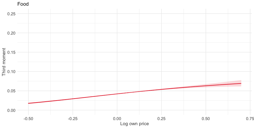
(a) Food: log own price

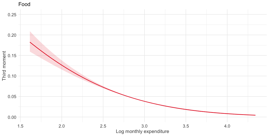
(b) Food: log household expenditure

Services

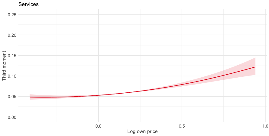
(c) Services: log own price

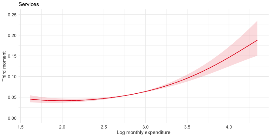
(d) Services: log household expenditure

Figure D.1: Third moments of budget shares

D.3 Estimates welfare changes

D.3.1 Estimation

From the estimated moments of the budget shares, we can calculate all required price and income derivatives needed to make the results in Theorem 3 and Corollary 1 operational. In particular, from the chain rule and the dominated convergence theorem, it holds that

$$\begin{split}\frac{\partial M_{k1}(\mathbf{p},y)}{\partial p_{k}}&=\frac{y}{p_{k}^{2}}\left[\frac{\partial W_{k1}(\mathbf{p},y)}{\partial\log p_{k}}-W_{k1}(\mathbf{p},y)\right],\\ \frac{\partial M_{k1}(\mathbf{p},y)}{\partial y}&=\frac{y}{p_{k}}\left[\frac{\partial W_{k1}(\mathbf{p},y)}{\partial\log y}+W_{k1}(\mathbf{p},y)\right],\\ \frac{\partial M_{k2}(\mathbf{p},y)}{\partial y}&=\frac{y}{p_{k}^{2}}\left[\frac{\partial W_{k2}(\mathbf{p},y)}{\partial\log y}+2W_{k2}(\mathbf{p},y)\right],\end{split}$$

and

$$\begin{split}\frac{\partial M_{k2}(\mathbf{p},y)}{\partial p_{k}}&=\frac{y^{2}}{p_{k}^{3}}\left[\frac{\partial W_{k2}(\mathbf{p},y)}{\partial\log p_{k}}-2W_{k2}(\mathbf{p},y)\right],\\ \frac{\partial M_{k3}(\mathbf{p},y)}{\partial y}&=\frac{y^{2}}{p_{k}^{3}}\left[\frac{\partial W_{k3}(\mathbf{p},y)}{\partial\log y}+3W_{k3}(\mathbf{p},y)\right].\end{split}$$

D.3.2 Heterogeneity by household expenditure

Table D.4 presents the relative deviation between our estimate and the first-order approach by decile of household expenditure.

	Food		Services
Expenditure decile	Estimate (%)	90% CI	Estimate (%)	90% CI
	Our estimate
1	-3.37	[-3.67, -3.09]	-4.13	[-4.56, -3.76]
2	-3.90	[-4.19, -3.65]	-3.84	[-4.26, -3.49]
3	-4.13	[-4.42, -3.87]	-3.68	[-4.11, -3.33]
4	-4.31	[-4.59, -4.05]	-3.54	[-3.98, -3.19]
5	-4.46	[-4.76, -4.20]	-3.41	[-3.85, -3.08]
6	-4.62	[-4.91, -4.36]	-3.26	[-3.67, -2.96]
7	-4.76	[-5.06, -4.51]	-3.11	[-3.51, -2.81]
8	-4.93	[-5.23, -4.68]	-2.92	[-3.31, -2.64]
9	-5.14	[-5.43, -4.89]	-2.67	[-3.03, -2.39]
10	-5.50	[-5.79, -5.26]	-2.23	[-2.65, -1.84]
	RA estimate
1	-3.43	[-3.75, -3.17]	-4.32	[-4.75, -3.94]
2	-3.98	[-4.27, -3.72]	-4.05	[-4.47, -3.70]
3	-4.23	[-4.51, -3.97]	-3.93	[-4.35, -3.58]
4	-4.42	[-4.70, -4.16]	-3.82	[-4.25, -3.48]
5	-4.58	[-4.87, -4.33]	-3.72	[-4.16, -3.38]
6	-4.75	[-5.04, -4.50]	-3.62	[-4.06, -3.28]
7	-4.91	[-5.20, -4.66]	-3.51	[-3.95, -3.17]
8	-5.08	[-5.37, -4.83]	-3.40	[-3.81, -3.07]
9	-5.29	[-5.58, -5.03]	-3.25	[-3.64, -2.95]
10	-5.64	[-5.94, -5.38]	-3.10	[-3.48, -2.74]

Table D.4: Relative deviation between our average estimate and the first-order approach by decile of household expenditure

D.4 Decomposition of the aggregate price index

Similar to Corollary 1, we can decompose the second-order contribution to average welfare into four terms:

$$\begin{split}\mathbb{E}[CV^{\omega}(p_{0},p_{1},y)]\approx\Delta pM_{1}(p_{0},y)+A_{1}+A_{2}+A_{3}+A_{4},\end{split}$$

where

$$\begin{split}A_{1}&=\frac{(\Delta p)^{2}}{2}\left(\frac{\partial}{\partial p}M_{1}(p_{0},y)+\frac{1}{y}(M_{1}(p_{0},y))^{2}\right),\\ A_{2}&=\frac{(\Delta p)^{2}}{2}\left[\frac{1}{2}\frac{\partial}{\partial y}(M_{1}(p_{0},y))^{2}-\frac{1}{y}(M_{1}(p_{0},y))^{2}\right],\\ A_{3}&=\frac{(\Delta p)^{2}}{2}\frac{1}{y}\left[M_{2}(p_{0},y)-(M_{1}(p_{0},y))^{2}\right],\\ A_{4}&=\frac{(\Delta p)^{2}}{2}\left[\frac{1}{2}\left(\frac{\partial}{\partial y}M_{2}(p_{0},y)-\frac{\partial}{\partial y}(M_{1}(p_{0},y))^{2}\right)-\frac{1}{y}\left(M_{2}(p_{0},y)-(M_{1}(p_{0},y))^{2}\right)\right].\\ \end{split}$$

To obtain this decomposition, we made use repeatedly of the fact that homothetic demands must satisfy $\frac{\partial}{\partial y}q^{\omega}(p_{0},y)=\frac{1}{y}q^{\omega}(p_{0},y)$.

Table D.5: Decomposition of the second-order contribution to the PI

		Food		Services
		Share (%)	90% CI	Share (%)	90% CI
$A_{1}$	RA/H	121.39	[119.67, 123.19]	80.11	[76.16, 82.52]
$A_{2}$	RA/NH	-25.40	[-27.18, -23.72]	13.48	[11.49, 16.59]
$A_{3}$	NRA/H	6.00	[5.70, 6.30]	6.62	[6.21, 7.16]
$A_{4}$	NRA/NH	-1.99	[-2.46, -1.49]	-0.20	[-0.71, 0.40]

(N)RA: (no) representative agent; (N)H: (non)-homothetic preferences

D.5 Decomposition variance CV

From Section 5.1, we know that the CV can be approximated as follows:

$$CV^{\omega}(p_{0},p_{1},y)=\Delta pq^{\omega}(p_{0},y)+\frac{(\Delta p)^{2}}{2}\left(\frac{\partial q^{\omega}(p_{0},y)}{\partial p}+q^{\omega}(p_{0},y)\frac{\partial q^{\omega}(p_{0},y)}{\partial y}\right)+O((\Delta p)^{3}).$$

We can therefore decompose the variance of the CV into

$$\begin{split}\text{Var}(CV^{\omega}(p_{0},p_{1},y))&\approx(\Delta p)^{2}\text{Var}(q^{\omega}(p_{0},y))+\frac{(\Delta p)^{4}}{4}\text{Var}\left(\frac{\partial q^{\omega}(p_{0},y)}{\partial p}+q^{\omega}(p_{0},y)\frac{\partial q^{\omega}(p_{0},y)}{\partial y}\right)\\ &+(\Delta p)^{3}\text{Cov}\left(q^{\omega}(p_{0},y),\frac{\partial q^{\omega}(p_{0},y)}{\partial p}+q^{\omega}(p_{0},y)\frac{\partial q^{\omega}(p_{0},y)}{\partial y}\right).\end{split}$$

When $\text{Var}(CV^{\omega}(p_{0},p_{1},y))<(\Delta p)^{2}\text{Var}(q^{\omega}(p_{0},y))$ and $\Delta p>0$, this implies that

$$\text{Cov}\left(q^{\omega}(p_{0},y),\frac{\partial q^{\omega}(p_{0},y)}{\partial p}+q^{\omega}(p_{0},y)\frac{\partial q^{\omega}(p_{0},y)}{\partial y}\right)<0.$$

References

- Aguiar and Serrano (2017) V. H. Aguiar and R. Serrano. Slutsky matrix norms: The size, classification, and comparative statics of bounded rationality. Journal of Economic Theory, 172:163–201, 2017.
- Allen and Rehbeck (2019) R. Allen and J. Rehbeck. Identification with additively separable heterogeneity. Econometrica, 87(3):1021–1054, 2019.
- Allen and Rehbeck (2020a) R. Allen and J. Rehbeck. Counterfactual and welfare analysis with an approximate model. arXiv preprint arXiv:2009.03379, 2020a.
- Allen and Rehbeck (2020b) R. Allen and J. Rehbeck. Satisficing, aggregation, and quasilinear utility. Available at SSRN 3180302, 2020b.
- Amini et al. (2021) A. Amini, Q. Sun, and N. Motee. Error Bounds for Carleman Linearization of General Nonlinear Systems, pages 1–8. 2021.
- Apesteguia and Ballester (2015) J. Apesteguia and M. A. Ballester. A measure of rationality and welfare. Journal of Political Economy, 123(6):1278–1310, 2015.
- Atkin et al. (2020) D. Atkin, B. Faber, T. Fally, and M. Gonzalez-Navarro. Measuring welfare and inequality with incomplete price information. Technical report, National Bureau of Economic Research, 2020.
- Baqaee and Burstein (2021) D. Baqaee and A. Burstein. Aggregate welfare and output with heterogeneous agents. Unpublished Note, 2021.
- Baqaee et al. (2022) D. Baqaee, A. T. Burstein, and Y. Mori. A new method for measuring welfare with income effects using cross-sectional data. NBER Working Paper, (w30549), 2022.
- Baqaee and Burstein (2022) D. R. Baqaee and A. Burstein. Welfare and output with income effects and taste shocks. The Quarterly Journal of Economics, 138(2):769–834, 2022.
- Bergemann and Bonatti (2019) D. Bergemann and A. Bonatti. Markets for information: An introduction. Annual Review of Economics, 11:85–107, 2019.
- Bergemann et al. (2022) D. Bergemann, A. Bonatti, and T. Gan. The economics of social data. The RAND Journal of Economics, 53(2):263–296, 2022.
- Bhattacharya (2015) D. Bhattacharya. Nonparametric Welfare Analysis for Discrete Choice. Econometrica, 83(2):617–649, 2015.
- Bhattacharya (2018) D. Bhattacharya. Empirical welfare analysis for discrete choice: Some general results. Quantitative Economics, 9(2):571–615, 2018.
- Bhattacharya and Komarova (2021) D. Bhattacharya and T. Komarova. Incorporating social welfare in program-evaluation and treatment choice. arXiv preprint arXiv:2105.08689, 2021.
- Blomquist et al. (2021) S. Blomquist, W. Newey, A. Kumar, and C.-Y. Liang. On bunching and identification of the taxable income elasticity. Journal of Political Economy, 129(8):2320–2343, 2021.
- Blundell and Matzkin (2014) R. Blundell and R. L. Matzkin. Control functions in nonseparable simultaneous equations models. Quantitative Economics, 5(2):271–295, 2014.
- Blundell and Powell (2003) R. Blundell and J. L. Powell. Endogeneity in Nonparametric and Semiparametric Regression Models, volume 2 of Econometric Society Monographs, page 312–357. Cambridge University Press, 2003.
- Blundell et al. (2008) R. Blundell, M. Browing, and I. Crawford. Best nonparametric bounds on demand responses. Econometrica, 76:1227–1262, 2008.
- Blundell et al. (2012) R. Blundell, J. L. Horowitz, and M. Parey. Measuring the price responsiveness of gasoline demand: Economic shape restrictions and nonparametric demand estimation. Quantitative Economics, 3(1):29–51, 2012.
- Blundell et al. (2003) R. W. Blundell, M. Browning, and I. A. Crawford. Nonparametric Engel Curves and Revealed Preference. Econometrica, 71(1):205–240, January 2003.
- Border (2003) K. C. Border. The integrability problem. Division of the Humanities and Social Sciences. California Institute of Technology, 2003.
- Burns and Ziliak (2016) S. K. Burns and J. P. Ziliak. Identifying the Elasticity of Taxable Income. The Economic Journal, 127(600):297–329, 03 2016.