Grid-Centric Traffic Scenario Perception for Autonomous Driving: A Comprehensive Review
Abstract
Grid-centric perception is a crucial field for mobile robot perception and navigation. Nonetheless, grid-centric perception is less prevalent than object-centric perception for autonomous driving as autonomous vehicles need to accurately perceive highly dynamic, large-scale outdoor traffic scenarios and the complexity and computational costs of grid-centric perception are high. The rapid development of deep learning techniques and hardware gives fresh insights into the evolution of grid-centric perception and enables the deployment of many real-time algorithms. Current industrial and academic research demonstrates the great advantages of grid-centric perception, such as comprehensive fine-grained environmental representation, greater robustness to occlusion, more efficient sensor fusion, and safer planning policies. Given the lack of current surveys for this rapidly expanding field, we present a hierarchically-structured review of grid-centric perception for autonomous vehicles. We organize previous and current knowledge of occupancy grid techniques and provide a systematic in-depth analysis of algorithms in terms of three aspects: feature representation, data utility, and applications in autonomous driving systems. Lastly, we present a summary of the current research trend and provide some probable future outlooks.
Index Terms:
Autonomous driving, grid-centric perception, occupancy flow, scene reconstruction, multi-modality fusionI Introduction
Safe operation of autonomous vehicles requires an accurate and comprehensive representation of the surrounding environment. Object-centric pipelines consisting of 3D object detection, multi-object tracking, and trajectory prediction are the dominant 3D automotive perception modules. Nevertheless, object-centric techniques may fail in open-world traffic scenarios where the shape or appearance of objects is not well-defined. These obstacles, also known as long-tail obstacles, include deformable obstacles, such as two-section trailers; special-shaped obstacles, such as overturned vehicles; obstacles of unknown categories, such as gravel on the road, garbage; partially obscured objects, etc. Thus, a more robust representation of these long-tail problems is urgently required. Grid-centric perception is believed to be a promising solution, as it is able to provide occupancy and motion of any position in 3D surrounding space without knowing an object. Lots of attention has been given to this area, recent progress demonstrates that it is still one of the most promising and challenging research topics in autonomous vehicles. To this end, we intend to provide a comprehensive review of grid-centric perception techniques.
forked edges,
for tree=
grow=east,
reversed=true,anchor=base west,
parent anchor=east,
child anchor=west,
base=left,
font=,
rectangle,
draw=hiddendraw, line width=0.6pt,
rounded corners,align=left,
minimum width=2.5em,
edge=black, line width=0.55pt,
l+=1.9mm,
s sep=7pt,
inner xsep=7pt,
inner ysep=8pt,
ver/.style=rotate=90, rectangle, draw=none, rounded corners=3mm, fill=red, text centered, text=white, child anchor=north, parent anchor=south, anchor=center, font=,,
level2/.style=rectangle, draw=none, fill=orange,
text centered, anchor=west, text=white, font=, text width = 7em,
level3/.style=rectangle, draw=none, fill=brown, fill opacity=0.8,text centered, anchor=west, text=white, font=, text width = 2.7cm, align=center,
level3_2/.style=rectangle, draw=none, fill=gray, fill opacity=0.8,text centered, anchor=west, text=white, font=, text width = 2.7cm, align=center,
level3_1/.style=rectangle, draw=none, fill=brown, fill opacity=0.8, text centered, anchor=west, text=white, font=, text width = 3.2cm, align=center,
level4/.style=rectangle, draw=red, text centered, anchor=west, text=black, font=, align=center, text width = 2.9cm,
level5/.style=rectangle, draw=red, text centered, anchor=west, text=black, font=, align=center, text width = 14.7em,
level5_1/.style=rectangle, draw=red, text centered, anchor=west, text=black, font=, align=center, text width = 26.1em,
level5_2/.style=rectangle, draw=red, text centered, anchor=west, text=black, font=, align=center, text width = 30.0em,
level5_3/.style=rectangle, draw=red, text centered, anchor=west, text=black, font=, align=center, text width = 35.0em,
,
where level=1text width=5em,font=,align=center,
where level=2text width=6em,font=,,
where level=3text width=6em,font=,where level=4text width=5em,font=,where level=5font=,[Grid-centric perception, ver
[OGM fundamentals
(Sec. -A ), level2 [Occupancy grid map (Sec. -A1); Continuous grid map (Sec. -A2) ; Dynamic grid map (Sec. -A3) , level5_3]]
[BEV 2D grid
(Sec. III), level2
[LiDAR BEV (Sec. III-A), level3
]
[Vision BEV (Sec. -B), level3
[Geometry-based PV2BEV (Sec. -B1); Network-based PV2BEV (Sec. -B2) , level5_1]
]
[Fusion (Sec. III-B), level3
[Multi-sensor fusion (Sec. III-B1); Multi-agent fusion (Sec. III-B2) , level5_1]
]]
[3D occupancy
(Sec. IV), level2
[LiDAR SSC (Sec: IV-A), level3
]
[Vision 3D (Sec: IV-B), level3
[Explicit voxel reconstruction (Sec. IV-B1); Implicit neural rendering (Sec. IV-B2) , level5_1]
]]
[Temporal tasks
(Sec. V ), level2 [Temporal BEV fusion(Sec. V-A); Short-term motion (Sec. V-B) ; Long-term occupancy flow (Sec. V-C) , level5_3]]
[Efficient learning
(Sec. VI), level2
[multitasking (Sec: VI-A), level3
[Joint BEV Seg&Motion (Sec. VI-A1); Joint 3D Det& BEV Seg (Sec. VI-A2);
More multitasking (Sec. VI-A3), level5_1]
]
[Label-efficient
(Sec: VI-B), level3
]
[Computation-efficient
(Sec: VI-C), level3
[Memory-efficient (Sec. VI-C1); Efficient PV2BEV (Sec. VI-C2) , level5_1]
]]
[Grid applications
in AD systems
(Sec. VII), level2
[Industrial design
(Sec: VII-A), level3
]
[Related perception tasks
(Sec: VII-B), level3
[SLAM (Sec. VII-B1); Map element detection (Sec. VII-B2) , level5_1]
]
[Grid-based Planning
(Sec: VII-C), level3
[Graph search (Sec. VII-C1); Collision detection (Sec. VII-C2)
States in RL (Sec. VII-C3); End-to-end planning (Sec. VII-C4) , level5_1]
]]
]
Grid mapping has been widely acknowledged as an essential prerequisite for the safe navigation of mobile robots and autonomous vehicles. Beginning with the well-established occupancy grid map (OGM), the surrounding area is partitioned into uniform grid cells. The value of each cell represents the belief of occupancy, which is crucial and efficient for collision avoidance. With the development of deep neural networks, grid-centric methods are developing rapidly and now generate a more comprehensive understanding of semantics and motion than conventional OGM. In summary, modern grid-centric methods are able to predict the belief of occupancy, semantic categories, future motion displacement, and instance information of each grid cell. The outputs of grid-centric methods are on the real-world scale, fixed to the ego pose coordinate. In this manner, the grid-centric perception becomes an important prerequisite that supports downstream driving tasks such as risk assessment and vehicle trajectory planning.
The significant advantages of grid-based representations over object-based representations are as follows: insensitive to obstacle’s geometric shape or semantic category, and stronger resistance to occlusion; ideal for multi-modal sensor fusion as a uniform space coordinate for different sensors to align with; robust uncertainty estimation, as each cell stores the joint probability of the existence of different obstacles. However, the primary drawback of grid-centric perception is the high complexity and computational burden.
Existing surveys about automotive perception including 3D object detection[1], 3D object detection from images[2], Neural Radiance Field(NeRF)[3], vision-centric BEV perception[4, 5], cover parts of the techniques in grid-centric perception. However, perception tasks, algorithms, and applications that center on grid representation are not thoroughly discussed in these evaluations. We present a comprehensive overview of grid-centric perception methods for autonomous vehicle applications, as well as an in-depth study and systematic comparison of grid-centric perception from various modalities and categories of approaches. We emphasize perception techniques based on real-time deep learning-based algorithms rather than offline mapping techniques such as multi-view stereo (MVS)[6, 7]. For feature representation, we cover both the explicit mapping of BEV and 3D grids, as well as emerging implicit mapping techniques like NeRF[8]. We investigate grid-centric perception in the context of the entire autonomous driving system, including its temporal tasks in temporally-consistent data sequences, multitasking, efficient learning, and connections to downstream tasks. The contributions of this paper is summarized as follows:
-
1.
To the best of our knowledge, we provide the first comprehensive review of the grid-centric perception methods from various perspectives for autonomous driving.
-
2.
We provide a structural and hierarchical overview of grid-centric perception techniques. Both academic and industry perspectives on the grid-centric perception of autonomous driving practices are analyzed.
-
3.
We summarize the observation of the current trend and provide future outlooks for grid-centric perceptions.
As illustrated in Fig. 1, this paper is organized in a hierarchically-structured taxonomy. In addition to the background and OGM basics, we focus on four core issues in the taxonomy, the spatial representation of features, the temporal expression of features, efficient algorithms, and the application of grid-centric perception within autonomous driving systems. Section. II introduces the background of grid-centric perception, including task definition, commonly used datasets, and metrics. Section. III discusses techniques for projecting multi-modal sensors to BEV feature space, as well as the associated 2D BEV grid tasks. Section. IV discusses representing full scene geometry in 3D voxel grids, including LiDAR-based semantic scene completion (SSC) and camera-based semantic scene reconstruction. Section. V introduces temporal modules designed for aggregation of historical grid features and short- or long-term panoptic occupancy prediction. Section VI presents efficient multi-task models and computation-efficient grid models and fast operators that are crucial for parallel computing on grids. Section. VII introduces practices of grid-centric perception in autonomous driving system from both academia and industry. Section. VIII presents several future outlooks for state-of-the-art grid-centric perception techniques. Section. IX concludes this paper. A review of well-established non-deep-learning OGM and its variants in the field of autonomous driving, including discrete occupancy grid, continuous occupancy grid, and dynamic occupancy grid, is provided in the supplementary materials. In order to avoid overlapping with recent vision BEV perception surveys[4, 5], the process of lifting image features to BEV is also briefly discussed in the supplementary materials.
II Background
This section introduces tasks formulation, commonly used datasets and metrics of grid-centric perception.
II-A Task Definition of Grid-Centric Perception
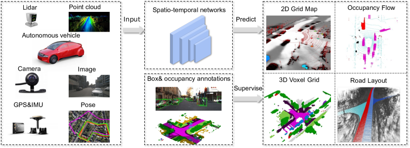
Grid-centric perception refers to the concept that, given the multi-modality input of on-board sensors, algorithms need to transform raw information to BEV or voxel grids and preform various perception tasks on each grid cells. A general formula of grid-centric perception can be represented as:
| (1) |
where is a set of the past and future grid-level representation, and represents one or more sensory inputs. How to represent grid attributes and grid features are two crucial problems in this task. An illustration of grid-centric perception process is shown in Fig. 2.
Sensory inputs. Autonomous vehicles rely heavily on multiple cameras, LiDAR sensors, and RADAR sensors for environmental perception. The camera system may consist of monocular cameras, stereo cameras, or both. It is relatively cheap and provides high-resolution images , including texture and color information. However, cameras cannot obtain direct 3D structural information and depth estimation. In addition, image quality is highly dependent on environmental conditions.
LiDAR sensors generate a 3D representation of the scene in the form of a point cloud , where is the number of points in the scene and each point contains the coordinates, as well as extra attributes such as reflective intensity. Due to depth perception, a broader field of view, and a greater detection range, LiDAR sensors are utilized more frequently in autonomous driving and are less susceptible to environmental conditions. Unfortunately, the applications are mainly limited by cost.
RADAR sensors are one of the most significant sensors in autonomous driving due to their low cost, long detection range, and ability to detect moving targets in adverse environments. RADAR sensors return points containing the relative locations and velocities of the targets. However, RADAR data is sparser and more sensitive to noise. Hence, autonomous vehicles frequently combine RADAR data with other sensory inputs to provide additional geometrical information. It is believed that 4D imaging radar will become a key enabler for low-cost L4-L5 autonomous driving with significant improvements. 4D imaging radar is able to generate dense pointclouds with a higher resolution and estimate the height of objects[13, 14]. Seldom are 4D radar applications applied in grid-centric perception.
Comparisons with 3D object detection. 3D object detection focuses on representing common road obstacles using 3D bounding boxes, whereas grid-centric detection segments low-level occupancy and semantic cues for road obstacles. Grid-centric perception has several advantages: It loosens the restriction on the shape of obstacles and can describe articulated objects with variable shapes; it relaxes the typicality requirements of obstacles. It can accurately describe occupancy and motion cues for novel classes and instances, thus enhancing the system’s robustness. In the object detection domain, novel classes and instances can be partially handled by open-set[15] or open-world[16, 17, 18] detection techniques, but remain a long-tailed problem for object-centric perception.
II-A1 Geometric Tasks
2D occupancy grid mapping. OGM is a straightforward and practical task for modeling occupied and free space in the surrounding environment. Occupancy, which represents the belief of occupancy probability divided by free probability, is the central idea of OGM.
3D occupancy mapping. 3D occupancy mapping is defined as modelling occupancy in a volumetric space. A basic task is to use a voxel grid of equal-sized cubic volumes to discretize the mapped area[19].
II-A2 Semantic Tasks
BEV segmentation. BEV segmentation is defined as semantic or instance segmentation of BEV grids. The commonly segmented categories include dynamic objects (vehicles, trucks, pedestrians and cyclists) and static road layouts and map elements (lanes, pedestrian crossing, drivable areas, walkway).
Semantic scene completion. SemanticKITTI[20] dataset first defines the task of outdoor semantic scene completion. Given single-scan LiDAR pointclouds, the SSC task is to predict the complete scene inside a certain volume. In the scene around the ego vehicle, the volume is represented by uniform voxel grids, each of which possesses the property of occupancy (empty or occupied) and its semantic label.
II-A3 Temporal Tasks
BEV motion. The definition of BEV Motion task is to predict the short-term future motion displacement of each grid cell. That is, how far each grid cell may move in a brief time frame. Dynamic Occupancy Grid (DOG) is a supplementary of OGM that can model dynamic grid cells with two-directional velocity and the velocity uncertainty.
Occupancy flow. Long-term occupancy prediction extends standard OGM to flow fields with mitigates some drawbacks of trajectory-set prediction and occupancy. Occupancy flow task need to predict the motion and position probability of all agents in the flow fields. Waymo’s open dataset occupancy and flow challenge at the CVPR2022 workshop111https://waymo.com/open/challenges/2022/occupancy-flow-prediction-challenge/ stipulates that, given a one-second history of real agents in a scene, the task must predict the flow fields of all agents in eight seconds.
Comparisons with scene flow. The purpose of optical or scene flow is to estimate the motion of image pixels or LiDAR points from the past to the present. The scene flow method operates on the original domain of data. Since the spatial distribution of point clouds is not regular and it is difficult to determine the matching relationship between the point clouds of two successive frames, it is not simple to extract its true value, and the scene flow of point clouds encounters real problems. In contrast, after discretizing the two-dimensional space, BEV motion can apply fast deep learning components (such as 2D convolutional networks) so that flow fields operate under the real-time requirements of autonomous driving.
| Dataset | Year | Size(hr.) | Scenes | LiDAR scans | RGB images | Ann. frames | Annotations | Classes | Night/Rain | Views | Stereo | Locations | Auxiliary |
|---|---|---|---|---|---|---|---|---|---|---|---|---|---|
| KITTI[21] | 2012 | 1.5 | 22 | 15k | 15k | 15k | 200k | 8 | No/No | 1 | Yes | Germany | - |
| Lyft L5[22] | 2019 | 2.5 | 366 | 46k | 323k | 46k | 1.3M | 9 | No/No | 6 | No | USA | Maps |
| Argoverse[23] | 2019 | 0.6 | 113 | 44k | 490k | 22k | 993k | 15 | Yes/Yes | 7 | Yes | USA | Maps |
| SemanticKITTI*[20] | 2019 | - | 22 | 43k | - | - | 4549M* | 28 | -/- | - | - | Germany | - |
| nuScenes[24] | 2020 | 5.5 | 1000 | 400k | 1.4M | 40k | 1,4M | 23 | Yes/Yes | 6 | No | SG,USA | Maps,RADAR data |
| Waymo Open[25] | 2020 | 6.4 | 1150 | 230k | 1M | 230k | 12M | 23(4)** | Yes/Yes | 5 | No | USA | - |
| KITTI-360[26] | 2021 | - | - | 80k | 300k | - | 68k | 37 | -/- | 3 | Yes | Germany | - |
| Argoverse 2[27] | 2021 | - | 1000 | - | - | - | - | 30 | Yes/Yes | 9 | Yes | USA | Maps |
| ONCE[28] | 2021 | 144 | - | 1M | 7M | - | 417k | 5 | Yes/Yes | 7 | No | China | - |
II-B Datasets
Grid-centric methods are mostly conducted on existing large-scale autonomous driving datasets with annotations of 3D object bounding boxes, LiDAR segmentation labels, annotations of 2D&3D lane and high definition maps. Most influential benchmarks for grid-centric perception include KITTI[21], nuScenes[24], Argoverse[23], Lyft L5[22], SemanticKITTI[20], KITTI-360[26], Waymo Open Dataset (WOD)[25] and Once dataset[28]. Note that grid-centric perception is usually not a standard challenge for each dataset, therefore test sets are held out and most methods report their results on the validation set. Table. I provides a summary of these benchmarks’ information.
Future development of datasets for grid-centric perception. Current driving datasets are mostly intended for benchmarking fully-supervised closed-world object-centric tasks, which may impede the unique advantages of grid-centric perception. Future datasets may require a more varied open-world driving situation in which potential obstacles cannot be represented as bounding boxes. Argoverse2[27] dataset is a next-generation dataset for its 10Hz densely-annotated 1k sensor sequences with 26 categories and super large-scale, unlabeled 6M LiDAR frames.
II-C Evaluation Metrics
Metrics for BEV segmentation. For binary segmentation in conventional OGM, which classifies grids as occupied and free, most previous works use accuracy for a simple metric. For semantic segmentation, the primary metric is Intersection-over-Union (IoU) for each class and mean Intersection over Union (mIoU) over all classes. IoU between prediction and label writes:
| (2) |
Metrics for BEV prediction. MotionNet[12] encodes motion information by associating each grid cell with a displacement vector in a BEV map and proposes metrics for motion prediction by classifying non-empty grid cells into three velocity ranges: static, slow() and fast(). In each velocity range, the mean and median distances between the predicted displacements and the ground-truth displacements have been utilized.
FIERY[29] uses the Video Panoptic Quality (VPQ)[30] metric for prediction of future instance segmentation and motion in a BEV map. This metric is defined as:
| (3) |
where , , are the true positive, false positive and false negative instance predictions at timestep , is the future predition horizon. Notice that a true positive prediction has IoU over 0.5 with the ground truth and the same instance id as the ground truth throughout time.
Metrics for occupancy flow challenge. Waymo’s Occupancy Flow Challenge evaluates the ability of algorithms to predict occupancy distribution across a longer time span (8s). Metrics of occupancy flow consist of occupancy metrics, flow metric, and joint metrics. The primary occupancy metrics are Area under the Curve (AUC) and Soft Intersection over Union (Soft-IoU) [31]which are used for binary segmentation. AUC for class (vehicle/pedestrian) estimates the area under the PR-curve. The Soft-IoU metric for each class writes:
| (4) |
where are ground-truth and predicted occupancy at time step .
For flow metric, End-Point Error (EPE) measures the mean L2 distance between the ground-truth flow field and predicted flow field as:
| (5) |
where a flow field at time t holds motion vector for each pixel.
The joint metrics measure the accuracy of flow and occupancy predictions at each time step , so is used to warp the ground-truth occupancy () as:
| (6) |
where applies the flow field as a function to transform the occupancy. If the joint prediction is accurate enough, should be close to the ground-truth . Therefore, flow-grounded AUC and flow-grounded Soft-IoU have been employed.
Metrics for 3D occupancy prediction. The primary metrics for semantic scene completion is mIoU over all semantic classes. IoU, Precision and Recall are used on the scene completion to assess the geometrical reconstruction quality. 3D occupancy prediction challenge measures the F-score as the harmonic mean of the completeness and the accuracy , F-score is computed as follows:
| (7) |
where is the percentage of predicted voxels that are within a distance threshold to the ground truth voxels, and is the percentage of ground truth voxels that are within a distance threshold to the predicted voxels. All metrics are only evaluated in annotated space due to semi-dense ground truth in most real-world datasets.
III Bird’s-Eye View 2D Grid Representation
BEV grid is a common representation of obstacle detection for on-road vehicles. The basic technique for grid-centric perception is to map raw sensor information to BEV grid cells, which differ in mechanisms for different sensor modalities. LiDAR point clouds are naturally represented in 3D space, so there is a long-standing tradition of extracting point or voxel features on BEV maps[32, 33]. Cameras are rich in semantic cues but lack geometric cues, which makes 3D reconstruction an ill-posed problem. Considering that the algorithms used to project image features from perspective view to BEV view (PV2BEV) have been comprehensively discussed in recent reviews[4, 5], we present recent advances of PV2BEV algorithms related to BEV grids in supplementary materials.
III-A LiDAR-based Grid Mapping
Feature extraction of LiDAR point clouds follows the following paradigms: point, voxel, pillar, range view, or hybrid feature from above[1]. This section focuses on the feature mapping of point clouds to BEV grids.
LiDAR data collected in 3D space can be easily transformed to BEV and fused with information from multi-view cameras. The sparse and variable density of LiDAR point clouds renders CNNs inefficient. Some methods [34, 35, 36] voxelize the point cloud into a uniform grid and encode each grid cell with hand-crafted features. MV3D[34], AVOD[35] generates the BEV representation by encoding each grid with height, intensity, and density features. BEV representation in PIXOR[36] is a combination of the 3D occupancy tensor and the 2D reflectance map, which keep the height information as channels. BEVDetNet[37] further reduces BEV-based model latency to 2ms on Nvidia Xavier embedded platform. For advanced temporal tasks on grids, MotionNet proposes a novel spatial-temporal encoder STPN[12] which aligns past point clouds to the current ego pose. The network design is shown in Fig. 4.
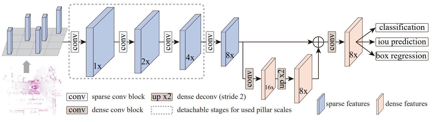
However, these fixed encoders are not successful in utilizing all the information contained within the point cloud. The learned features become a trend. VoxelNet[38] stacks voxel feature encoding (VFE) layers to encode point interactions within a voxel and generates a sparse 4D voxel-wise feature. And then VoxelNet uses a 3D convolutional middle layer to aggregate and reshape this feature and passes it through a 2D detection architecture. To avoid hardware-unfriendly 3D convolution, the pillar-based encoder in PointPillars[39] and EfficientPillarNet[40] learns features on pillars of the point cloud. The features can be scattered back to the original pillar positions to generate a 2D pseudo-image. PillarNet[41] further develops pillar representation by fusing densified pillar semantic features with spatial features in the neck module for final detection with orientation-decoupled IoU regression loss. The encoder for PillarNet[41] is illustrated in Fig. 3.
III-B Deep Fusion on Grids
Multi-sensor multi-modality fusion has been a long-standing issue for automotive perception. Fusion frameworks are often categorized into early fusion, deep fusion, and late fusion. Among them, deep fusion has demonstrated the best performance in an end-to-end framework. Grid-centric representation serves as a unified feature embedding space for deep fusion among multiple sensors and agents.
III-B1 Multi-sensor Fusion
Cameras are geometry-loss but semantics rich, while LiDARs are semantics-loss but geometry rich. Radars are geometry and semantics sparse but robust to different weather conditions. Deep fusion fuses latent features across modalities and compensates for the limitations of each sensor.
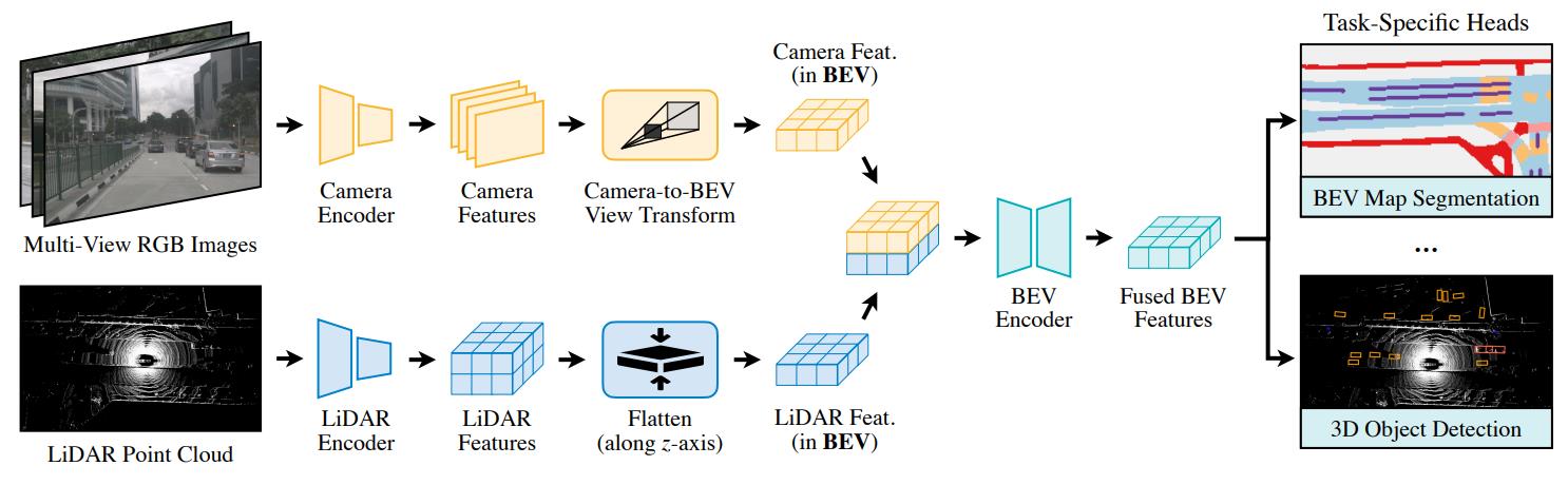
LiDAR-camera fusion. Some methods perform the fusion operation at a higher 3D level and support feature interaction in 3D space. UVTR[45] samples features from the image according to predicted depth scores and associates features of point clouds to voxels according to the accurate position. Thus, the voxel encoder for cross-modality interaction in voxel space can be introduced. AutoAlign[46] designs a cross-attention feature alignment module (CAFA) to enable the voxelized feature of point clouds to perceive the whole image and perform feature aggregation. Instead of learning the alignment through the network in AutoAlign[46], AutoAlignV2[47] includes a cross-domain DeformCAFA and employs the camera projection matrix to obtain the reference points in the image feature map. FUTR3D[48] and TransFusion[49] fuses features based on attention mechanism and queries. FUTR3D employs a query-based modality-agnostic feature sampler(MAFS) to extract multi-modal features according to 3D reference points. TransFusion relies on LiDAR BEV features and image guidance to generate object queries and fuses these queries with image features. A simple and robust approach is to unify fusion on BEV features. Two implementations of BEVFusion[50, 51], shown in Fig. 5 unify features from multi-modal inputs in a shared BEV space. DeepInteration[52] and MSMDFusion[53] designs multi-model interaction in BEV space and voxel space to better align spatial features from different sensors.
Camera-radar fusion. Radar sensors are originally designed for Advanced Driving Assistance System (ADAS) tasks, so their accuracy and density are insufficient for use in high-level autonomous driving tasks. OccupancyNet[54] and NVRadarNet[55] only use radars to perform real-time obstacle and free space detection. Camera-radar fusion is a promising low-cost perception solution that supplements semantics to radar geometry. Simple-BEV[56], RCBEVDet[57], and CramNet[58] have investigated different approaches for radar feature expression on BEV and fusion with vision BEV features. RCBEVDet[57] process the multi-frame aggregated radar point clouds with a PointNet++[59] network. CramNet[58] sets the camera features as query and radar features as value to retrieve radar features along the pixel ray in 3D space. Simple-BEV[56] voxelizes multi-frame radar point clouds as a binary occupancy image and uses meta-data as additional channels. RRF[60] yields a 3D feature volume from each camera by projection and sampling and then concatenates a rasterized radar BEV map. It finally gets a BEV feature map by reducing the vertical dimension.
Lidar-camera-radar fusion. LiDAR, radar, and camera fusion is a robust fusion strategy for all weathers. RaLiBEV[61] adopts an interactive transformer-based bev fusion that fuses LiDAR point clouds and radar range azimuth heatmaps. FishingNet[62] uses top-down semantic grids as a common output interface to conduct late fusion of the LiDAR, radars and cameras and performs short-term prediction of semantic grids.
III-B2 Multi-agent Fusion
Recent works on grid-centric perception are mostly based on single-agent systems, which have limitations in complex traffic scenes. Advancements in Vehicle-to-Vehicle(V2V) communication technologies enable vehicles to share their sensory information. CoBEVT[63] is the first multi-agent multi-camera perception framework that can generate BEV segmented maps cooperatively. In this framework, the ego vehicle geometrically warps the received BEV features according to the pose of the sender and then fuses them using a transformer with fused axial attention (FAX). Dynamic occupancy grid map (DOGM) also shows the capacity of reducing uncertainty in the fusion platform for multi-vehicle cooperative perception[64, 65, 66].
IV 3D Occupancy Mapping
While BEV grids simplify the vertical geometry of dynamic scenes, 3D grids are able to represent the full geometry of driving scenes with a rather low resolution, including the road surface and the shape of obstacles, at the expense of higher computation costs. LiDAR sensors are naturally suitable for 3D occupancy grids, but there are two major issues for point cloud input: The first challenge is inferring full scene geometry from points reflected at the surface of obstacles. The second is inferring dense geometry from sparse LiDAR inputs. Camera-based methods are emerging in 3D occupancy mapping. Images are naturally dense in pixels but need depth maps to be converted to 3D occupancy.
| Method | Year |
IoU |
Road(15.30%) |
Sidewalk(11.13%) |
Parking(1.12%) |
Other-ground(0.56%) |
Building(14.10%) |
Car(3.92%) |
Truck(0.16%) |
Bicycle(0.03%) |
Motorcycle(0.03%) |
Other-vehicle(0.20%) |
Vegetation(39.30%) |
Trunk(0.51%) |
Terrain(9.17%) |
Person(0.07%) |
Bicyclist(0.07%) |
Motorcyclist(0.05%) |
Fence(3.90%) |
Pole(0.29%) |
Traffic-sign(0.08%) |
mIoU |
|---|---|---|---|---|---|---|---|---|---|---|---|---|---|---|---|---|---|---|---|---|---|---|
| SSCNet[68]a | 2017 | 29.8 | 27.6 | 17.0 | 15.6 | 6.0 | 20.9 | 10.4 | 1.8 | 0.0 | 0.0 | 0.1 | 25.8 | 11.9 | 18.2 | 0.0 | 0.0 | 0.0 | 14.4 | 7.9 | 3.7 | 9.5 |
| SSCNet-full[67]b | - | 50.0 | 51.2 | 30.8 | 27.1 | 6.4 | 34.5 | 24.6 | 1.2 | 0.5 | 0.8 | 4.3 | 35.2 | 18.2 | 29.0 | 0.2 | 0.2 | 0.0 | 19.9 | 13.1 | 6.7 | 16.1 |
| TS3D[69]a | 2019 | 29.8 | 28.0 | 17.0 | 15.6 | 4.9 | 23.2 | 10.7 | 2.4 | 0.0 | 0.0 | 0.2 | 24.7 | 12.5 | 18.3 | 0.0 | 0.0 | 0.0 | 13.2 | 7.0 | 3.5 | 9.5 |
| TS3D+DNet[20] | - | 25.0 | 27.5 | 18.5 | 18.9 | 6.6 | 22.0 | 8.0 | 2.2 | 0.1 | 0.0 | 4.0 | 19.5 | 12.8 | 20.2 | 2.3 | 0.6 | 0.0 | 15.8 | 7.6 | 7.0 | 10.2 |
| TS3D+DNet+SATNet[20] | - | 50.6 | 62.2 | 31.6 | 23.3 | 6.5 | 34.1 | 30.7 | 4.8 | 0.0 | 0.0 | 0.1 | 40.1 | 21.9 | 33.1 | 0.0 | 0.0 | 0.0 | 24.0 | 16.9 | 6.9 | 17.7 |
| LMSCNet-singlescale[67] | 2020 | 56.7 | 64.8 | 34.7 | 29.0 | 4.6 | 38.1 | 30.9 | 1.5 | 0.0 | 0.0 | 0.8 | 41.3 | 19.9 | 32.0 | 0.0 | 0.0 | 0.0 | 21.3 | 15.0 | 0.8 | 17.6 |
| S3CNet[70] | 2020 | 45.6 | 42.0 | 22.5 | 17.0 | 7.9 | 50.2 | 31.2 | 6.7 | 41.5 | 45.0 | 16.1 | 39.5 | 34.0 | 21.2 | 45.9 | 35.8 | 16.0 | 31.3 | 31.0 | 24.3 | 29.5 |
| JS3C-Net[71] | 2021 | 56.6 | 64.7 | 39.9 | 34.9 | 14.1 | 39.4 | 33.3 | 7.2 | 14.4 | 8.8 | 12.7 | 43.1 | 19.6 | 40.5 | 8.0 | 5.1 | 0.4 | 30.4 | 18.9 | 15.9 | 23.8 |
| Local-DIFs[72] | 2022 | 57.7 | 67.9 | 42.9 | 40.1 | 11.4 | 40.4 | 34.8 | 4.4 | 3.6 | 2.4 | 4.8 | 42.2 | 26.5 | 39.1 | 2.5 | 1.1 | 0.0 | 29.0 | 21.3 | 17.5 | 22.7 |
| MonoScene[9] | 2022 | 34.2 | 54.7 | 27.1 | 24.8 | 5.7 | 14.4 | 18.8 | 3.3 | 0.5 | 0.7 | 4.4 | 14.9 | 2.4 | 19.5 | 1.0 | 1.4 | 0.4 | 11.1 | 3.3 | 2.1 | 11.1 |
| MotionSC (T=1)[42]c | 2022 | 56.9 | 66.0 | 36.5 | 29.6 | 7.0 | 39.0 | 31.4 | 1.0 | 0.0 | 0.0 | 3.6 | 40.0 | 19.0 | 30.0 | 0.0 | 0.0 | 0.0 | 23.4 | 20.0 | 3.4 | 18.4 |
| TPVFormer[73] | 2023 | 34.2 | 55.1 | 27.2 | 27.4 | 6.5 | 14.8 | 19.2 | 3.7 | 1.0 | 0.5 | 2.3 | 13.9 | 2.6 | 20.4 | 1.1 | 2.4 | 0.3 | 11.0 | 2.9 | 1.5 | 11.3 |
| VoxFormer[74] | 2023 | 44.2 | 53.6 | 26.5 | 19.7 | 0.4 | 19.5 | 26.5 | 7.3 | 1.3 | 0.6 | 7.8 | 26.1 | 6.1 | 33.1 | 1.9 | 2.0 | 0.0 | 7.3 | 9.2 | 4.9 | 13.4 |
| OccDpeth[75] | 2023 | 45.1 | 61.7 | 30.9 | 27.5 | 9.6 | 25.4 | 25.6 | 5.5 | 1.4 | 2.2 | 4.2 | 26.0 | 11.4 | 26.5 | 2.5 | 2.6 | 0.7 | 18.4 | 10.0 | 9.7 | 15.9 |
IV-A LiDAR-based Semantic Scene Completion
Semantic scene completion (SSC) is a task of explicitly inferring the occupancy and semantics of uniform-sized voxels. The definition of SSC given by SemanticKITTI[20] is to infer the occupancy and semantics of every voxel grid based on a single-frame LiDAR point cloud. The past survey[76] thoroughly investigates both indoor and outdoor SSC datasets and methods. This section focuses on advances in SSC methods for autonomous driving. Detailed class-wise performance of existing methods on SemanticKITTI, with either LiDAR or camera as inputs, is presented in Table.II.
SemanticKITTI[20] is the first real-world outdoor benchmark for SSC. It reports the results of four baseline approaches based on SSCNet[68] and TS3D[69]. Since SSC relies heavily on contextual information, early methods start from U-Net architecture. SSCNet adopts flipped Truncated Signed Distance Function(fTSDF) to encode a single depth map as input and passes it through a 3D dense CNN. Built on SSCNet, TS3D combines semantic information inferred from the RGB image and voxel occupancy as the input of a 3D dense CNN. Note that LiDAR point clouds are more common input for autonomous driving than RGB-D sequences. SemanticKITTI benchmark therefore applies TS3D and SSCNet without fTSDF as baselines using range images from LiDAR instead of depth maps from RGB-D. The other two baselines modify TS3D by directly using labels from LiDAR-based semantic segmentation method and exchanging the 3D backbone with SATNet[77].
The dense 3D CNN blocks in SSCNet and TS3D leads to high memory and computation need and dilation of the data manifold. One alternative to address this issue is to take advantage of the efficiency of 2D CNN. LMSCNet[67] uses a lightweight U-Net architecture with 2D backbone convolution and 3D segmentation heads. Turning the height dimension into a feature dimension becomes a common practice for traffic scenes where the data mainly varies longitudinally and laterally. Pillar-based LMSCNet achieves good performance at speed and has the capability to infer multiscale SSC. Similarly, Local-DIFs[72] creates a BEV feature map of the point cloud and passes it through 2D U-Net to output feature maps at three scales which make up the novel representation of the 3D scene, continuous Deep Implicit Functions (DIFs). By querying the function for corner points of all voxels, Local-DIFs can be evaluated on SemanticKITTI benchmark and performs well on geometric completion accuracy.
Another promising alternative is to use sparse 3D networks, such as SparseConv[78] used in JS3C-Net[71] and Minkowski[79] used in S3CNet[70], which only operate on non-empty voxels. JS3C-Net is a sparse LiDAR point cloud semantic segmentation framework which regards SSC as an auxiliary task. It includes a point-voxel interaction(PVI) module to enhance this multi-task learning and promote knowledge transfer between two tasks. For semantic segmentation, it utilizes a 3D sparse convolution U-Net. The cascaded SSC module predicts a coarse completion result, which is refined in PVI module. Experiments show that JS3C-Net achieves state-of-the-art results on both tasks. S3CNet constructs sparse 2D and 3D feature from a single LiDAR scan and passes them throngh sparse 2D and 3D U-Net style network in parallel. To avoid applying dense convolutions in decoder, S3CNet proposes a dynamic voxel late fusion of BEV and 3D predictions to further densify the scene and then applys a spatial propagation network to refine the result. In particular, it achieves impressive results in rare classes of SemanticKITTI.
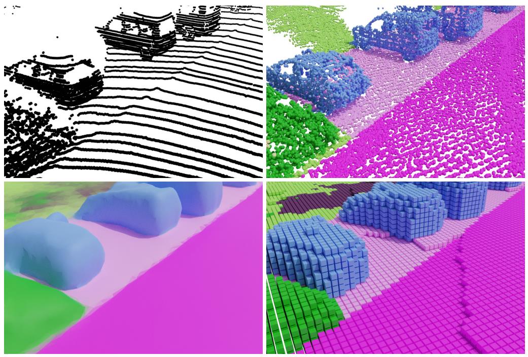
Limitation of label formulation. As existing outdoor SSC benchmarks[20, 26] generate labels from aggregation multi-frame semantic pointclouds, traces of dynamic objects are unavoidable interference in labels, dubbed sptaio-temporal tubes. Due to a large number of parked vehicles in SemanticKITTI, all existing SSC methods predict dynamic objects as if they are static and are punished by benchmark metrics. To address the problem of inaccuracies of ground truth and focus on SSC in the instant of the input, Local-DIFs[72] propose a dataset variant based on SemanticKITTI by only keeping the single instant scan on dynamic objects and removing free space points within the shadows of dynamic objects. Besides, Local-DIF can continuously represent scenes to avoid artifacts caused by discretization, as shown in Fig. 6. Wilson et al.[42] develops a synthetic outdoor dataset CarlaSC without occlusions and traces surrounding the ego vehicle in CARLA[80]. They propose a real-time dense local semantic mapping method, MotionSC[42] which conbines a spatial-temporal backbone of MotionNet[12] and the segmentation head of LMSCNet[67]. Note that MotionSC which ignores temporal information also performs well on SemanticKITTI benchmark. Recently, TPVFormer[73] replaces dense voxel grid labels with sparse LiDAR segmentation labels for supervision of dense semantic occupancy from surround-view cameras. Compared to voxel labels with fixed resolution, point cloud labels are more easily accessible (mature for annotation and auto-labeling), and they can serve as supervision for voxel grids with arbitrary perception range and resolution.
IV-B Camera-based Semantic Scene Reconstruction
IV-B1 Explicit Voxel-based Networks
Different from the offline mapping method represented by structure from motion (SFM), online perception which projects pixels into three-dimensional space is a new task. Camera-based SSC methods do not perform as well as other LiDAR-based methods on SemanticKITTI benchmark due to lack of geometrical information and the narrower FOV of the camera. The recent new labels for nuScenes helps better performance of vision-centric methods. MonoScene[9] is the first outdoor 3D voxel reconstruction framework based on monocular camera. It uses dense voxel labels from SSC task for evaluation metrics. It includes a module for 2D feature line of sight projection(FLoSP) to bridge 2D and 3D U-Net, as well as a 3D context relation prior(CRP) layer for enhancing learning of contextual information. VoxFormer[74] is a two-stage transformer-based framework, which starts from sparse visible and occupied queries from depth map and then propagate them to dense voxels with self-attention. OccDepth[75] is a stereo-based method which lifts stereo features to 3D space via a stereo soft feature assignment module. It uses a stereo depth network as teacher model to distill depth-augmented occupancy perception module as student model. Unlike above methods that require dense semantic voxel labels, TPVFormer[73] is a the first surround-view 3D reconstruction framework which only uses sparse LiDAR semantic labels as supervision. TPVFormer generalizes BEV to Tri-Perspective View (TPV), which means feature expression of 3D space through three slices perpendicular to the axis. It queries 3D points to decode occupancy with arbitrary resolution.
Vision-centric 3D occupancy prediction is still in its early stage of development. To promote the research of vision-centric 3D occupancy prediction, CVPR 2023 Workshops, end-to-end autonomous driving workshop222https://opendrivelab.com/e2ead/cvpr23 and vision-centric autonomous driving workshop333https://www.vcad.site/##/ hold 3D occupancy prediction as track 3 in autonomous driving challenges444https://opendrivelab.com/AD23Challenge.html##Track3.
IV-B2 Implicit Neural Rendering
Implicit neural representation (INR) is to represent all kinds of visual signals with continuous functions. As a groundbreaking new paradigm, Neural Radiance Field (NeRF) is attracting growing attention in the fields of computer graphics and computer vision due to its two unique features: self-supervised and photo-realistic. Although vanilla NeRF focuses on view rendering rather than 3D reconstruction, further researches explore NeRF’s ability to model 3D scenes, objects and surfaces. NeRF is widely used in human avatar and urban scene construction for driving simulators. Urban Radiance Field[81] reconstructs urban-level scenes with LiDAR supervision. Block-NeRF[82] divides the streets into blocks and trains each MLP block respectively.
The application of NeRF in 3D perception is still under-explored and challenging, as traffic scenarios perception requires fast, few-shot, generalizable NeRF with high depth estimation precision in unbounded scenes. SceneRF[83] introduces a probabilistic ray sampling strategy to represent continuous density volume with a mixture of gaussians and explicitly optimize depth. SceneRF[83] is the first self-supervised single-view large-scale scene reconstruction with NeRF. Behind the Scenes[84] proposes density fields to predict a volumetric scene representation with a single view input. The predicted density field, which detaches color with geometry, is able to predict not only ray termination depth but also BEV occupancy. It can also generalize well to unseen scenarios. CLONeR[85] fuses explicit occupancy grids and implicit neural representation with OGM using camera for colour and semantic cues and LiDAR for occupancy cues. In summary, hybrid representation of explicit voxel occupancy grid and implicit NeRF is a promising solution for modeling street-level scenes.
V Temporal Grid-Centric Perception
Since autonomous driving scenarios are temporally consecutive, leverage of multi-frame sensor data to get spatio-temporal features and decoding of motion cues are important issues for grid-centric perception. Sequential information are natural enhancement of observations of the real world. The main challenge of motion estimation is that, different from object-level perception which can easily associate newly detected objects with past trajectories, no explicit correspondence relation exists for grids, which increases the difficulty of accurate velocity estimation.
V-A Temporal Module for Sequential BEV Features
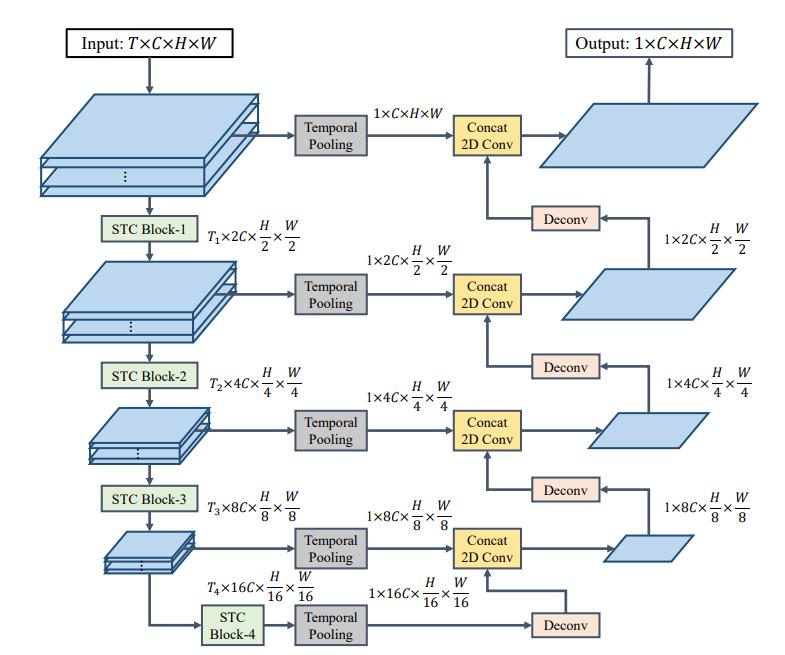
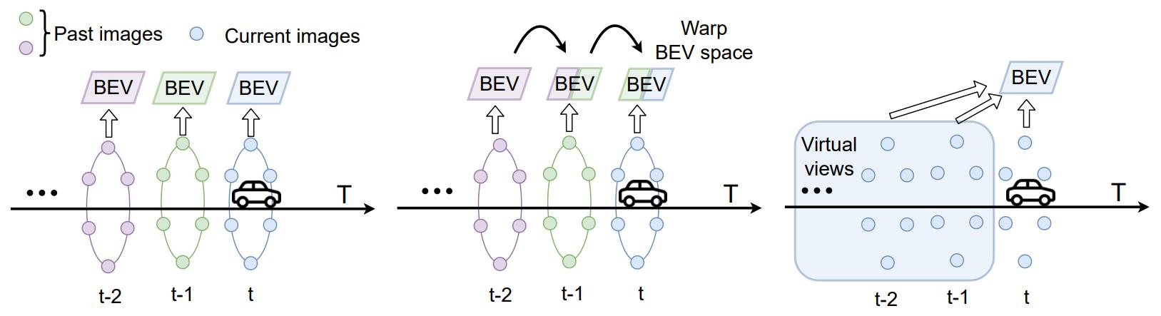
Most practices warp BEV features to the current frame by designing temporal fusion blocks. The core idea of wrapped-based method is to wrap and align BEV spaces at different timestamps based on ego-pose of vehicles. Different temporal aggregation methods are illustrated in Fig.7. Early arts[86, 87, 29] uses simple convolutional blockes for temporal aggregation. BEVDet4D[88] concatenates the wrapped spaces together. BEVFormer[89] uses deformable self-attention to fuse wrapped BEV spaces. UniFormer[90] argues wrapped-based methods are inefficient serial methods that do not support long-range fusion, and loses valuable information at the edge of perception range. To this end, UniFormer proposes attention in virtual views between current BEV and cached past BEV which can fuse larger perception range and better model long-range fusion.
V-B Short-term Motion Prediction
Tasks and Networks. With regard to different sensor modalities, short-term motion prediction is described into two formulations. For LiDAR-centric methods, the task is to predict motion displacement only on nonempty pillars during the next 1.0s. This formulation puts more emphasis on per-grid velocity. A basic network design consists of a spatial-temporal encoder and several BEV decoders. For vision-centric methods, the common task is to predict instance flow for the next 2.0s. This formulation focuses more on future occupancy state rather than grid velocity. A basic network design consists of an image encoder, a view projector, temporal aggregation modules, prediction modules and several BEV decoders.
Labels Generation. Common practices to generate the labels of grid flow (scene flow) comes from post-processing of adjacent frames of 3D bounding boxes with unique instance ids.
Backbone of spatial-temporal networks. Point clouds lies naturally in 3D space and can be aggregated on data level. The aggregation needs accurate positioning, which may be collected from high-precision GNSS equipments or point cloud registration method(e.g. ICP[91], NDT[92]), to convert the point cloud coordinates to the current ego vehicle coordinate system. The feature extraction backbone, with multi-frame point clouds as input, is able to simultaneously extract information in both spatial and temporal dimension to reduce computation load. A compact design is to voxelize pointclouds, treats pointclouds as pseudo BEV maps and vertical information as features on each BEV grids[12, 93, 94]. MotionNet proposes a light-weight and efficient spatio-temporal pyramid network (STPN) to extract spatio-temporal features. BE-STI proposes TeSE and SeTE to perform bidirectional enhancement of features. TeSE is for spatial understanding of each individual frame. SeTE is for high-quality motion cues by spatial discriminative features.
On the other hand, it is not practical to transform multi-frame images to current coordinate in raw data level. Therefore, spatial and temporal modules are designed seperately in vision-centric models. Spatial module design includes a universal image backbone and a view projector neck. The temporal module aligns temporally past multi-frame BEV features to the current ego pose mentioned in section V-A. Wrap-based methods, including FIERY[29], StretchBEV[95], BEVerse[96], ST-P3[97] are mainstream temporal backbone for feature representation.
Prediction module for vision-centric methods. Occupancy flow prediction needs state representation of future BEV features. Main components of prediction module are variants of recurrent neural networks (RNN). FIERY[29] proposes Spatial Gate Recurrent Unit (SpatialGRU) for propogating current BEV state to the near future. ST-P3[97] proposes Dual Pathway Probabilistic Future Modelling (DualGRU) which inputs two different distribution of current BEV states for stronger features of prediction. BEVerse[96] features iterative flow for efficient future prediction, which inputs last-frame BEV feature to current-frame prediction. StretchBEV adopts a variantional autoencoder from neural ordinary differential equations(Neural-ODE) to learn temporal dynamic through a generative approach.
Prediction head and loss design. LiDAR-centric methods. Decoders for motion inputs BEV feature from spatial-temporal backbones. The heads consists of 1-2 stacks of ConvBlock . The predicted heads in MotionNet[12] include cell classification head for category estimation, motion head for velocity estimation and state estimation head for classifying dynamic or static grids. BE-STI[94] features class-agnostic motion prediction head, which further exploits semantics to more accurate motion prediction. Loss design. In general, the spatial regression loss regresses the motion displacement in a L1 or MSE norm manner. Cross entropy loss is used for classification. As consistency is inherently guaranteed by sequential data, MotionNet[12] proposes a spatial consistency loss for cells belonging to the same object, and foreground temporal consistency loss for temporal constraint on motions between two consecutive frames. As a self-supervised framework, PillarMotion[93] proposes a self-supervised structural consistency loss to approximate pillar motion field and cross-sensory loss as an auxiliary regularization to complement the structural consistency given sparse LiDAR inputs.
Vision-centric methods. Existing methods follows the design in FIERY[29]. The prediction head consists of a lightweight BEV encoder (e.g. ResNet18[98]) and four BEV decoders. The five independent decoders output centerness, BEV segmentation, offset to the centers,and future flow vectors, respectively. The post-processing unit associates offsets with centers to form an instance from segmentation and outputs an instance flow from multi-frame instances. The spatial regression loss regresses the centers, offsets and future flows in a L1 or MSE norm manner. Cross entropy loss is used for classification. The probabilistic loss regresses the Kullback-Leibler divergence between BEV features.
V-C Long-term Occupancy Flow
We introduce non-end-to-end occupancy prediction in the farther future given ground-truth history objects as long-term occupancy flow task. The flow field on OGM domains combines two most commonly-used representations for motion forecasting: trajectory sets and occupancy grids. The main function of occupancy flow is to trace occupancy from far-future grids to current time locations using sequential flow vectors. DRF[99] uses auto-regressive sequential networks to predict occupancy residuals. ChauffeurNet[100] supplements safer trajectory planning with a multi-tasking learning of occupancy. Rules of the Road[101] proposes a dynamic framework to decode trajectories from occupancy flow. MP3[102] predict motion vectors and their corresponding possibility of each grid. The top three participants of the Waymo occupancy flow challenge are HOPE[103], VectorFlow[104], and STrajNet[105]. HOPE is a novel hierarchical spatio-temporal network with a multi-scale aggregator enriched with latent variables. VectorFlow[104] benefits from combining vectorized and rasterized representation. STrajNet[105] features interaction-aware transformer between trajectory features and rasterized features.
VI Efficient Learning for Grid-Centric Perception
Algorithms in autonomous driving scenarios are sensitive to multiple performance factors such as efficiency accuracy, memory, latency and label availability. For model efficiency, compared to previous modular system design where one module is responsible for one perception task, a multi-tasking model with a shared large backbone and several task-specific prediction heads are more welcomed in the industrial employment. For label efficiency, grid labels are expensive for annotation, which mainly comes from per-point annotation on LiDAR point clouds, so label-efficient learning techniques are urgently needed. For computation efficiency, since computing on grids are usually time and memory consuming, structures for efficient representation of voxel grids and operators for speeding up voxel-based operations are introduced.
VI-A Multi-task Models
Many researches reveal that predicting geometric, semantic and temporal tasks together in a multi-task model improves accuracy of each respective model. Recent advances handles more perception tasks other than grid-centric tasks in one base framework. A unified framework on BEV grids is efficient for an automotive perception system, this section introduces some commonly used multi-task learning frameworks.
VI-A1 Joint BEV Segmentation and Prediction
Accurate recognition of moving objects in BEV grids is an important prerequisite for BEV motion prediction. Therefore, past practices have demonstrated that accurate semantic recognition helps motion and velocity estimation. Common practices includes a spatial-temporal feature extraction backbone and task-specified heads, segmentation head to classify to which class the grid belongs, state head to classify stationary or dynamic grid, instance head which can predict offset of each grid to an instance center and motion head to predict short-term motion displacement. Vision-centric BEV models usually jointly optimize instances’ category, location and coverage, FIERY[29] introduces uncertainty loss[106] to balance the weight of segmentation, centerness, offset and flow losses.
Comparison with LiDAR and camera-based BEV Segmentation and Motion. An apparent difference is that LiDAR models estimate only grids accessible to laser scans. In other words, LiDAR-based methods have no completion ability for unobserved grid areas, or unobserved parts of dynamic objects. On the contrary, camera-based methods has techniques like probabilistic depth in LSS[107] which can infer some kinds of occluded geometry behind observations. Hallucinating Beyond Observation[108] is an example practice for inferring 3D shape of vehicles from images. Another difference is the generalization towards open-world unknown obstacles. MotionNet[12] states that although trained on closed-set labels, MotionNet has the ability to predict motion of unknown labels which are all categorized into the ’other’ class. However, camera-based methods are strict to classify well-defined semantics such as vehicle and pedestrian. Adaptability to open-world semantics of cameras remains an open question.
VI-A2 Joint 3D Object Detection and BEV Segmentation
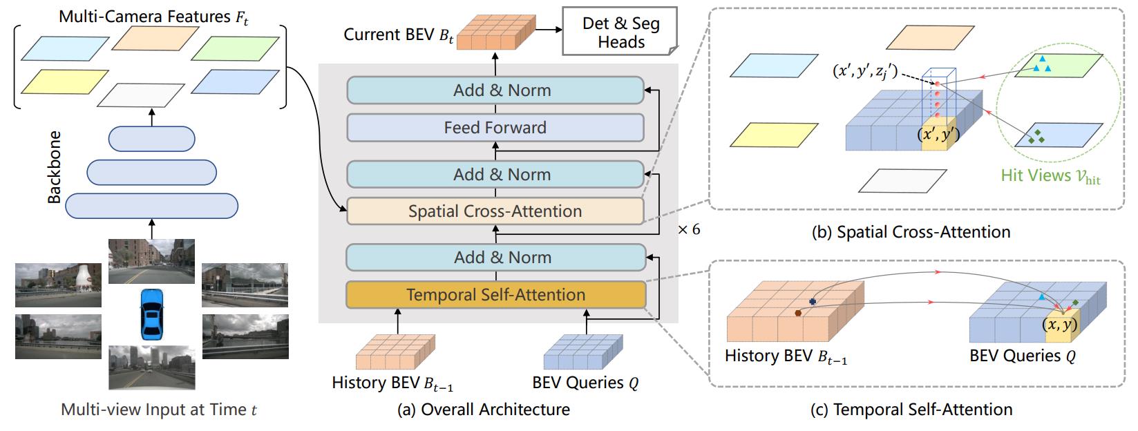
Joint 3D object detection and BEV segmentation is a popular combination which handles perception of dynamic objects and static road layout in one unified framework. It is also one of the tracks held by SSLAD2022 workshop challenge555https://sslad2022.github.io/pages/challenge.html. Given a shared BEV feature representation, common prediction heads for object detection are center head introduced in CenterPoint[109] and DETR head introduced in Deformable DETR[110], and common heads for segmentation are simple lightweight convolutional head (e.g.) and SegFormer[111] or Panoptic SegFormer[112] in BEVFormer[89], or can easily extend to more complicated segmentation techniques. The pipeline of BEVFormer is shown in Fig. 8. MEGVII proposes the first place solution[113] in SSLAD2022 multi-tasking challenge. They propose a multi-modal multi-task BEV model as a base. The model is pretrained on ONCE dataset and finetuned on AutoScenes dataset with techniques such as semi-supervised label correction and module-wise expotional moving average (EMA).
VI-A3 Multi-tasking for More Tasks
Recent researches places more major perception tasks in a BEV-based multi-tasking framework. BEVerse[96] shows a metaverse of BEV features with 3D object detection, road layout segmentation and occupancy flow prediction. Perceive Interact Predict[114] conducts end-to-end trajectory prediction based on interaction with map elements extracted online with shared BEV features. UniAD[115] is a comprehensive integration of object detection, tracking, trajectory prediction, map segmentation, occupancy and flow prediction, and planning, all in one vision-centric end-to-end framework. For more stable performance, UniAD is trained in two stages, tracking and mapping in the first stage and the whole model in the second stage.
Antagonism in multitask BEV models. A unified BEV feature representation and task-specified prediction heads compose an efficient framework design which is popular for industrial application. There remains a concern, whether the shared backbone strengthens each respective task. Joint BEV Segmentation and Motion researches[94] report a positive influence of multi-tasking: better segmentation leads to better motion prediction. However, most joint BEV detection and segmentation models[89, 114, 113] report the antagonism between two tasks. A reasonable explanations is that these two tasks are not relevant as they require features in different height, on the ground surface and above the ground. How shared BEV feature can generalizes well to fit each task needs adaption of specified feature maps remains an under-explored question.
VI-B Label-efficient Grid Perception
With the great success of large-scale pre-training in the field of natural language processing (NLP), self-supervised visual learning has received wider attention. In 2D domain, self-supervised models based on contrastive learning[116], based on masked image modeling[117, 118] are developing rapidly and is able to even surpass fully-supervised conterparts. In 3D domain, self-supervised pretraining have been conducted on LiDAR pointcloud[119, 120, 121, 122]. The core issue for self-supervised tasks is to design a predefined task for stronger feature representation. The predefined task may originate from temporal consistency, discriminative constractive learning and generative masked learning.
2D or 3D grids serve as satisfactory intermediate for self-supervised learning 3D geometry and motion. Voxel-MAE[123, 124] defines a voxel-based task which masks 90% of nonempty voxels and aims at completing them. This pretraining has boosted performance for downstream 3D object detection. Similarly, BEV-MAE[125] proposes to mask BEV grids and recover them as a predefined task. MAELi[126] distinguishes between free and occluded space and leverages a novel masking strategy to fit the inherent spherical projection of LiDARs. MAELi shows a significant improvement on performance of downstream detection tasks compared to other MIM-based pretraining. ALSO[127] sets a novel pre-defined task which predicts the 3D occupancy of query points which are sampled along each ray from the origin to the reflected point. For each ray two points close to the reflected point, one outside as free and one inside the surface as occupied, are sampled as query points. This pre-defined task is able to complete the obstacles’ surfaces and shows improvement in both 3D detection and LiDAR segmentation tasks.
The mutual supervision of LiDARs and cameras is effective for learning geometry and motion. PillarMotion[93] computes pillar motion in LiDAR branch, and optical flow compensated by ego pose. The optical flow leads to probabilistic motion masking. The optical flow and pillar flow undergo the cross-sensor regulation for a better structural consistency. Fine-tuning of PillarMotion also improves the semantics and motion of BEV grids.
For camera-based 3D vision, self-supervised monocular depth estimation has a long tradition. MonoDepth2[128] jointly predicts ego pose and depth map from monocular videos in a novel view synthesis manner. SurroundDepth[129] uses cross-view transformer(CVT) to capture clues between different cameras and uses pseudo depth from structure from motion operators. Instead of focusing on appearance and depth on image plane, NeRF[8] seems a promising approach for geometric self-supervision of camera-only 3D vision. As an early practice, SceneRF[83] studies novel view and depth synthesis by refining a MLP radiance field which can infer depth of source frame image with other frames in one sequence.
VI-C Computation-efficient Grid Perception
VI-C1 Memory-Efficient 3D Grid Mapping
Memory is the major bottleneck for 3D occupancy mapping in large-scale scenes with small resolution. There are several explicit mapping representations, such as voxel, mesh, surfel, voxel hashing, Truncated Signed Distance Fields (TSDF) and Euclidean Signed Distance Fields (ESDF). The vanilla voxel occupancy grid map queries storage by index, which needs high memory loads, so it is not usual in mapping methods. Mesh stores surface information about obstacles Surfel consists of points and patches, which include radii and normal vectors. Voxel hashing is a memory-efficient improvement of vanilla voxel methods, which only divides voxel on the scene surface measured by the camera, and stores the voxel block on the scene surface in the form of a hash table to facilitate the query of voxel block. Octomap[19] introduces an efficient probabilistic 3D mapping framework based on octrees. Octomap iteratively divides the cube space into eight small cubes, with the large cube becoming the parent node and the small cube becoming the child node, and the octopus tree can continuously expand down until it reaches a minimum resolution, called a leaf node. Octomap uses probabilistic descriptions to easily update node status based on sensor data.
Continuous mapping algorithms is another alternative for computation- and memory-efficient 3D occupancy description with arbitrary resolution. Gaussian Process Occupancy Maps (GPOM) uses the modified Gaussian process as a non-parametric Bayesian learning technique that introduces dependencies between points on the map for continuity. Hilbert Maps[130] projects the raw data into Hilbert space, where the logistic regression classifier is trained. BGKOctoMap-L[131] extends the traditional counting model CSM, and after smoothing it with a nuclear function, observations of surrounding voxels can be taken into account. AKIMap[132] is based on BGKOctoMap, and the point of improvement is that the kernel function is no longer radial based, adaptively changing direction and adapting to boundaries. DSP-map[133] generalizes particle-based map into continuous space and builds a continuous 3D local map adaptable for both indoor and outdoor applications. Broadly speaking, MLP structure in NeRF series is also an implicit continuous mapping for 3D geometry with almost no storage needs.
VI-C2 Efficient View Transformation from PV to BEV
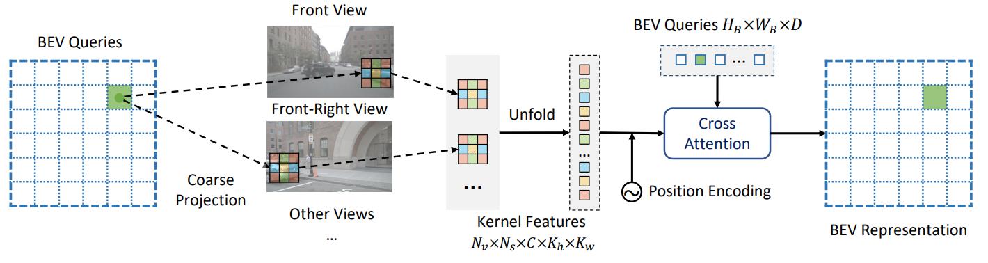
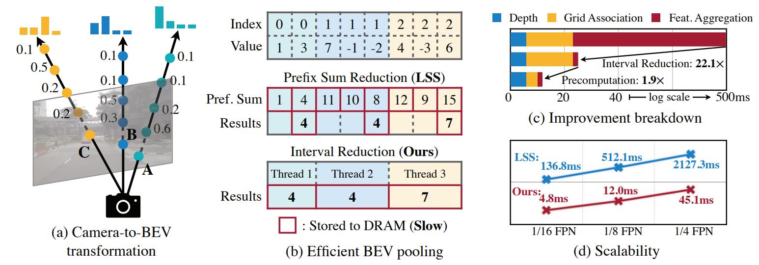
Vanilla LSS needs complex voxel computation on aligning probabilistic depth feature on BEV space, some arts[134, 50, 135] optimizes the computation cost of vanilla LSS[107] in designing efficient operators on voxel grids. LSS[107] leverages a cumsum traick which sorts frustum features to their unique BEV IDs, which is inefficient in sorting process over BEV grids. BEVFusion[50] proposes an efficient, exact without approximation, BEV pooling by precomputation of grid indices, and interval reduction via a specialized GPU kernel that parallelizes over BEV grids. BEVDepth[135] proposes efficient voxel pooling which assigns each frustum feature a CUDA thread and corresponds each pixel point to that thread. GKT[134] leverages the geometric priors to guide the transformer to focus on discriminative regions, and unfolds kernel features to generate BEV representation. For fast inference, GKT introduces a look-up table indexing for camera’s calibrated parameter-free configuration at runtime. Fast-BEV[136] is the first real-time BEV algorithm which proposes two acceleration designs based on M2BEV[137]. One is to pre-compute the projection index of BEV grids and the other is to project to the same voxel feature. Implementation details of GKT and BEVFusion are shown in Fig. 9, and Fig. 10.
VII Grid-Centric Perception in Driving Systems
Gird-centric perception provides other modules of autonomous driving with rich perceptual information. This section introduces a typical industrial design for a grid perception system, as well as several related perception fields and downstream planning tasks based on grid inputs.
VII-A Industrial Design of Grid-Centric Pipelines
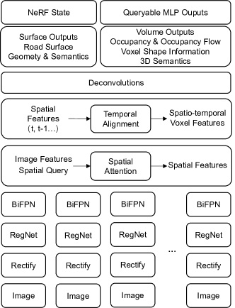
Tesla is a pioneer in the investigation of real-time occupancy networks with high performance and low latency at on embedded FSD computers. Tesla first introduces Occupancy Network[138] at the CVPR2022 Workshop on Autonomous Driving (WAD)[139], followed by the entire pipeline of grid-centric perception system at Tesla AI Day 2022[140]. The Occupancy Network’s model structure is depicted in Fig.11. First, the model’s backbone uses RegNet[141] and BiFPN[142] to obtain features from multiple cameras; then, the model performs an attention-based multi-camera fusion of 2D image features through spatial query with 3D spatial position. The model then executes temporal fusion by aligning and aggregating 3D feature space according to the provided ego pose. After fusing features across temporal horizons and deconvolution modules, the decoder decodes both volume and surface states. The combination of voxel grids and neural implicit representation is also noteworthy. Inspired by NeRF, the model concludes with an implicit queryable MLP decoder that accepts arbitrary coordinate values to decode information regarding the position of that space, i.e. occupancy, semantics, and flow. In this way, Occupancy Network is able to achieve arbitrary resolution for 3D occupancy mapping.
VII-B Related Perception Tasks
VII-B1 Simultaneous Localization and Mapping
The technique of Simultaneous Localization and Mapping (SLAM) is essential for mobile robots to navigate in an unknown environment. SLAM is highly related to geometry modeling. In the LiDAR SLAM field, High Order CRFs[143] proposes an incrementally constructed 3D scrolling OGM for efficiently representing large-scale scenarios. SUMA++[144] directly employs RangeNet++[145] for LiDAR segmentation, semantic ICP[91] only for stationary environments, and semantic-based dynamic filter for surfel map reconstruction. In the visual SLAM field, ORB-SLAM[146] stores maps with points, lines or planes. Diving the space into discrete grids is commonly used in dense and semantic mapping algorithms[147]. An new trend is to combine neural fields with SLAM with two advantages: NeRF models manipulate raw pixel value directly without feature extraction; NeRF model can differentiate both implicit and explicit representation, leading to a full-dense optimization of 3D geometry. NICE-SLAM[148] and NeRF-SLAM[149] are able to generate dense, hole-free maps. NeRF-SLAM generates a volumetric NeRF whose dense depth loss is weighted by the depth’s marginal covariance.
VII-B2 Map Element Detection
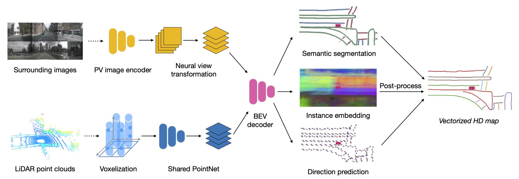
Detecting map elements is a crucial step in the production of high-definition maps. Traditional global map construction requires an offline global SLAM with a globally consistent pointcloud and centermeter-level localization. In recent years, a novel approach has been an end-to-end online learning approach based on BEV segmentation and post-processing techniques for local map learning, and then connecting local maps in different frames to produce a global high definition map[87]. The entire pipeline is depicted in Fig. 12.
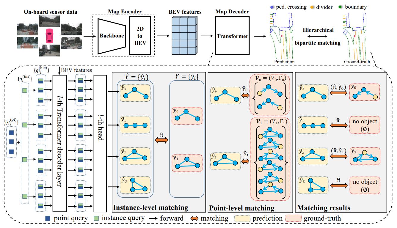
Typically, vectorized map elements are required for HD map-based applications, such as localization or planning. In HDMapNet[87], vectorized map elements can be generated through post-processing of BEV segmentation of map elements; however, end-to-end approaches have recently gained favor. End-to-end pipelines consist of feature extraction of on-board LiDARs and cameras introduced in Section III and transformer-based heads which regress vector element candidates as queries and interact with values in the BEV feature map. STSU[86] extracts road topology from a structured traffic scene by utilizing a Polyline-RNN[150] that extracts initial point estimates to form the centerline curves. VectorMapNet[151] directly predicts a sparse set of polylines primitives to represent the geometry of HD maps. InstaGram[152] proposes a hybrid architecture with CNN and graph neural network (GNN), which extracts vertex locations and implicit edge maps from BEV features. A GNN is utilized to vectorize and connect the HD map’s elements. As depicted in Fig. 13, MAPTR[153] proposes a hierarchical query embedding scheme to encode instance-level and point-level bipartite matching for map element learning.
VII-C Grid-Centric Perception for Planning
Occupancy grid typically conveys a description of risk or uncertainty in the scene’s comprehension, so it has a long history of serving as a prerequisite for the decision and planning module. In the field of robotics, grid-centric methods have higher-resolution details for collision avoidance when compared to object-centric methods. Recent advances enable grid-level motion prediction and end-to-end learning for planning.
VII-C1 Graph Search Based Planners on OGM
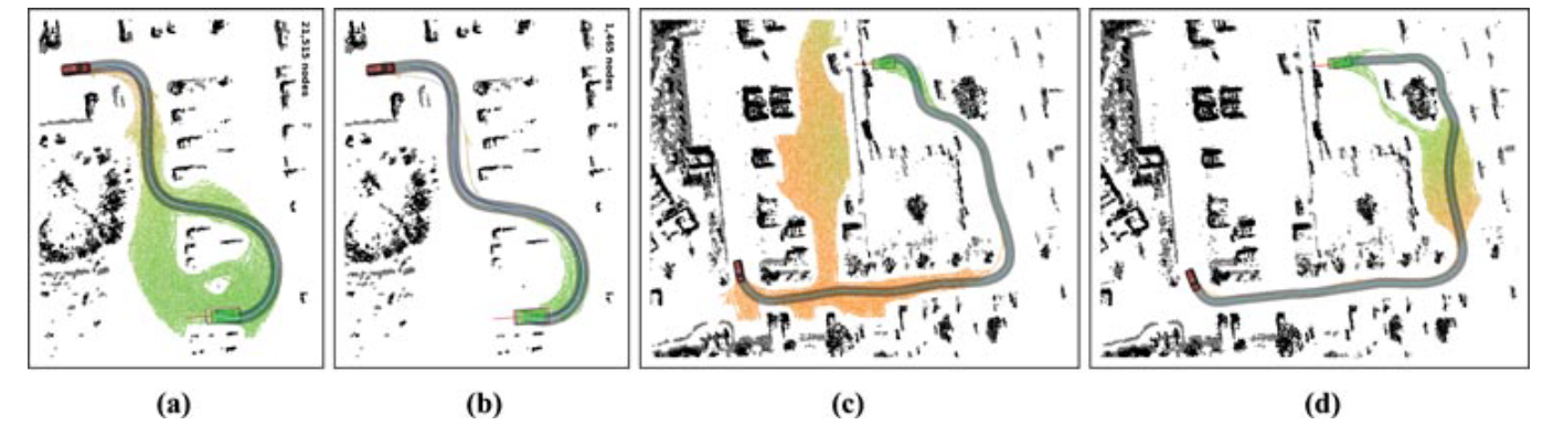
Motion Planning is intended to provide a trajectory comprised of a series of the vehicle’s states, while occupancy grid is a natural discrete presentation of the state space and the environment. To quantify the various state dimensions, additional OGM channels can be stacked. Therefore, the connections between the discrete grid cells constitute a graph, and the problem can be solved with graph searching algorithms[154], such as Dijkstra[155] and A*[156]. Junior[157] builds a four-dimensional grid including position, heading angle, and moving direction, and then proposes hybrid A* to find the shortest path for free-form scenarios such as parking lots and U-turns. The hybrid A* algorithm along with the result is illustrated in Fig. 14. Hall et al.[158] scans the expansion space in each row of OGM ahead of the ego vehicle in order to connect the nodes into a feasible trajectory with the lowest cost and deviation, which is a greedy strategy of graph searching in essence.
VII-C2 Collision Detection of Sampled Trajectories on OGM
In light of the vast amount of time required to search for a trajectory in the configuration space, sampling-based planners are proposed to sample a set of candidate trajectories and evaluate their feasibility and optimality. The collision avoidance constraint emphasizes the awareness of drivable space. Grid-centric representation provides more specific occupancy cues than element list representation, which increases the safety of collision detection.
Collision avoidance on 2D occupancy grid. OGM has long been recognized as a necessity for the collision avoidance of ground vehicles operating in outdoor environments. Fig. 15 illustrates a detection paradigm for 2D OGM collisions. Occupancy information is inherently stored as collision probability, but OGM/DOGM are discrete and dependent on grid size, making them unsuitable for continuous risk assessment. To this end, Dynamic Lambda-fields[159] proposes a framework for resolution-independent generic risk estimation.
Collision avoidance on 3D occupancy grid. Aerial robots require a comprehensive understanding of the full geometry of 3D voxel grids. To achieve this, Voxblox[161] incrementally builds ESDF from TSDF, which serves an efficient representation that is safe enough for collision avoidance of aerial robots and can run in real-time on a single CPU core.
Comparison of OGM-based planning for robotics and autonomous driving. OGM has many applications in robot navigation, but far fewer in autonomous driving planning. Siciliano et al.[162] noted that OGM is incapable of representing a single obstacle as a whole, resulting in problems with repeated expression and calculation. Therefore, although autonomous vehicles and robot decision-making planning are similar in essence, and OGM also has the robustness advantage in unknown scenarios, the autonomous vehicle faces a highly dynamic, complex element type road environment, and has high real-time requirements, so the shortcomings of OGM form a strong constraint in planning. Pertinent Boundry-based Unified Decision (PBUD)[163] system is therefore proposed as a unified planning framework with pertinent vector-space boundary generated from semantic and dynamic occupancy grid maps.
VII-C3 State Representation in RL Planners
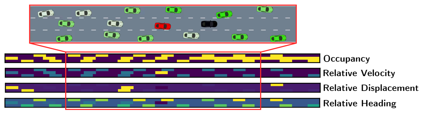
There has been extensive application of reinforcement learning (RL) algorithms, which formulate the planning problem as a Markov Decision Process. State is an essential component that must be accurately modeled for faster convergence and improved performance. The primitive element representation is incapable of maintaining permutation invariance and independence from the number of vehicles, whereas the occupancy grid representation can eliminate these constraints[164]. Mukadam et al.[165] utilize a history of binary occupancy grids to represent external environment information and concentrate it with the internal state as input. Numerous techniques[166, 167] extend the occupancy grid map with additional channels for other characteristics, such as velocities, headings, lateral displacements, and so on. As shown in Fig.16, kinematic parameters are integrated to provide the RL network with more information. Instead of a high-resolution grid representation, You et al.[168] focus on nine grid cells with the coarse-grained size of a vehicle.
VII-C4 End-to-end Planning
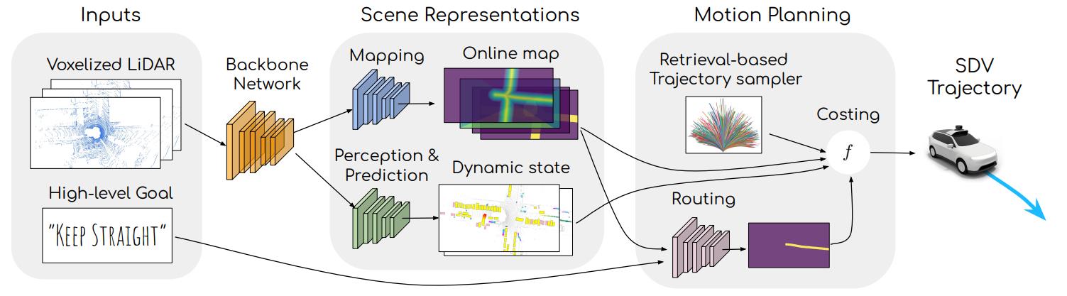
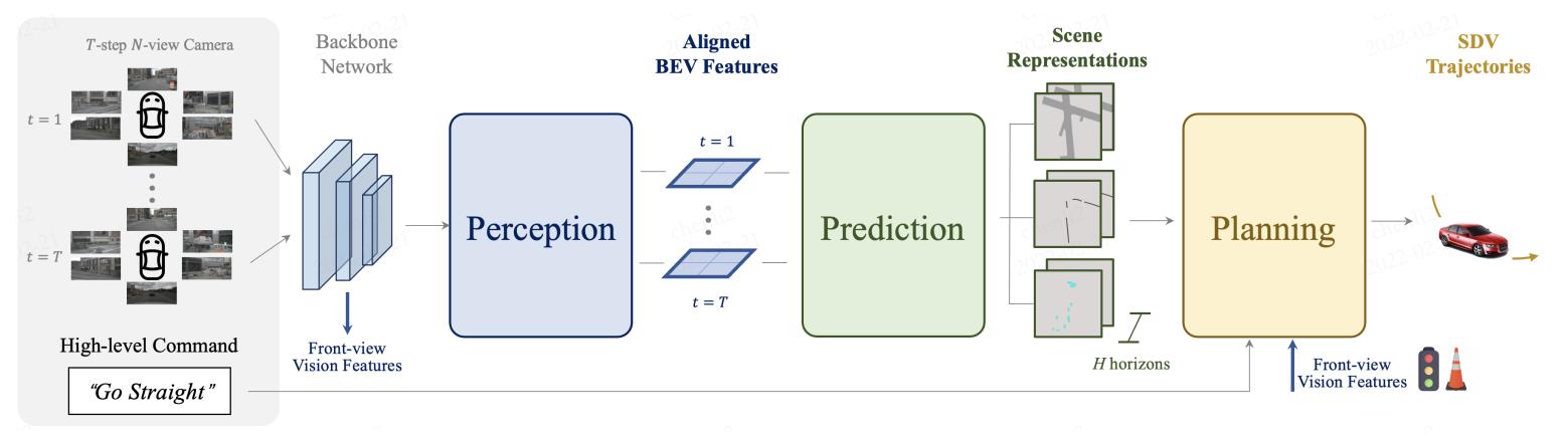
End-to-end planning on BEV features typically refers to the estimation of a cost map indicating a risk distribution over sampled template trajectories. Neural Motion Planner[169] conditions on LiDAR pointclouds and high-definition maps, extracts LiDAR BEV features, constructs cost-volume on BEV, and scores appropriate trajectories with minimal loss. LSS[107] interprets its camera-only end-to-end planning as ’shoot’. The shooting process is conceptualized as a classification of a collection of trajectories. MP3[102] uses occupancy flow in the context of a planning task but does not provide a direct analysis of the quality and performance of their motion forecasting technique. ST-P3[97] is the first framework to consider BEV motion in planning framework to improve intermediate interpretability. This is in response to the fact that past end-to-end planning methods did not consider future prediction. Two typical frameworks, MP3 planning with LiDAR and ST-P3 planning with cameras are shown in Fig. 17 and Fig. 18.
VIII Discussion
In this section, we present an in-depth summary of the current trend of grid-centric perception and provide a few future outlooks for the directions of further development.
VIII-A Observation of Current Trend
Compared with object-level perception tasks with predefined geometric primitives of on-road obstacles, grid-centric methods have no geometric assumptions, greater flexibility to describe objects with any shapes, and improved adaptation to occlusion situations. Grid-centric methods have become an integral component of today’s car perception systems. Three perspectives summarize the current trends.
Feature representation. Compared with the conventional OGM, deep learning has substantially improved the ability to describe the semantics and motion of grids. The ability to represent features is heavily dependent on the network structure. The representation of features from LiDAR, vision, and radar raw data to BEV grids has been investigated extensively. Grids are the natural foundation of spatial fusion, hence grid-based data-level fusion and feature-level fusion are effective in multi-sensor and multi-agent fusion scenarios. Deep learning-based 3D occupancy mapping has been extensively researched in lidar-based SSC methods, which generate dense scene geometry from a single LiDAR scan. However, vision-centric 3D occupancy prediction is becoming a trending topic, with both explicit mapping and implicit neural rendering being promising methods.
Data utility. Advanced automotive perception trains the neural networks on data sequences, or dubbed clips, rather than respective samples, so temporal information fusion and temporal tasks are vital for grid-centric perception. Occupancy flow has become an essential supplement for trajectory prediction as probabilistic parametric distribution on future occupancy reveals a better uncertainty description of future agents. Since autonomous driving perception operates on in-vehicle devices with very limited computing and storage resources, efficient learning and inference components must be designed. Industrial applications have implemented multi-task models and computation-efficient techniques. As grid labels are generally expensive, label-efficient learning, such as semi-, weakly-, or self-supervised learning, which is still in its infancy in 3D domains, is anticipated to accelerate the development of future solutions to handle open-world traffic scenarios.
Applications in driving systems. We also observe that grid-centric perception applications are playing an increasingly crucial role in autonomous driving systems as a whole. For the parallel tasks in the chain of autonomous driving, they share the requirements of geometry learning, where voxel or BEV grids have a great capacity for representation. There is a long history of grid-dependent planning for downstream tasks. An emerging trend is that end-to-end planning methods exhibit strong potential for conveying grid features to environment cognition modules and constructing more accurate safe fields.
VIII-B Future Outlooks
VIII-B1 Variable Granularity of Grids
In real-world driving scenarios, nearby surroundings usually have greater risk potentials than distant ones, necessitating increased vigilance as obstacles approach. In grid-centric perception, a natural demand is that nearby grids need higher resolution than distant grids. To step further, grids feature representations are still endowed with fixed granularity, which consumes more memory and computation on unnecessarily concerned areas (e.g. distant or occluded regions). Vision transformers and implicit representation are promising techniques for on-demand variable granularity. Another concern is to define the safe granularity for downstream tasks, as it is strongly tied to perception requirement analysis.
VIII-B2 4D NeRF for Dynamic Scenes
An important assumption of NeRF is the observation of static scenes. A common approach used in Urban Radiance Field[81] is to leverage other vision tasks(segmentation, detection) to filter out dynamic objects. AutoRF[170] uses monocular 3D object detection to learn radiance field representation on dynamic objects. Recent research has begun to investigate the 4D neural field that inherently considers the motion of dynamic scenes. Neural Scene Flow Field[171] first models the scene flow fields as a time-variant continuous function of appearance, geometry, and 3D scene motion. ENeRF[172] achieves photo-realistic real-time rendering of dynamic scenes for the first time and generalizes well to outdoor scenes. Due to the fact that the scenes of prior arts are not as complicated as traffic scenes in terms of scale and number of participants, an elegant 4D neural field suitable for highly complicated and dynamic traffic scenarios remains unexplored.
VIII-B3 Label-efficient Learning for Grid-Centric Perception
In comparison to object-centric perception, grid-centric perception requires more rigorous labeling. Dense voxel grids from multi-frame LiDAR semantic point cloud labels are rather expensive. In addition, LiDAR point clouds are constrained by a minimum angular resolution and a maximum height, meaning that distant obstacles may not be accurately marked. Label-efficient learning for 3D vision on grids is urgently needed. Weakly-supervised learning may involve learning from the occupancy of nearby objects and generalizing to remote obstacles. Self-supervised geometry learning and task-specified fine-tuning is another promising approach for label-efficient geometry learning.
VIII-B4 Open-world Occupancy for Vision-Centric Grids
The LiDAR has a straightforward geometric representation of line-of-sight and occupied regions. Once the ground is distinguished from other scene point clouds, the LiDAR-based general object detection (GOD) is able to detect unknown objects of any shape. Nevertheless, cameras lack accurate geometric cues of occupancy. Hence, the evaluation of space occupancy is highly dependent on semantic classification, and camera-based prediction is likely to fail when faced with novel semantic classes and novel instances. Self-supervised depth estimation is a preliminary method for obstacle detection without the need for semantics.
VIII-B5 Volumetric Flow Prediction
Grid flow is intended to be a concise and general representation of scene flow. BEV grid flow can only represent 2D motion, regardless of the possibility of 3D motion. Volumetric flow is a future further solution for accurate perception of 3D dynamic objects and stationary environments. Volumetric flow is capable of predicting motion flow vectors at any 3D location and knows that there are moving objects even if it doesn’t know their exact categories.
IX Conclusion
This paper provides a comprehensive review and analysis of the well-established and emergent grid-centric perception of autonomous driving. The background begins with an introduction of the problem definition, datasets, and evaluation metrics for grid-centric perception. For the most commonly used BEV 2D grids, feature representations for various sensors including LiDARs, cameras, and radars and multi-modal fusion are presented. In addition, we step further 3D grid representation, which includes LiDAR-based semantic scene completion and camera-based explicit reconstruction and implicit representation. For advances in temporal modules in grid-centric perception, we review sequential aggregation of historical information, short-term motion prediction, and long-term occupancy flow. Afterward, we provide a thorough investigation of efficient learning in grid-centric perception fields, which includes model-efficient multitask frameworks, label-efficient learning algorithms, memory-efficient 3D mapping structures, and computation-efficient voxel-based operators. We review the role of grid-centric perception in the whole autonomous driving system, industrial designs, related perception tasks, and connections with planning methods. Finally, we present a summary of current research trend and future outlooks for grid-centric perception. The authors hope that this paper will prospect the future development and deployment of grid-centric perception on autonomous driving vehicles.
Acknowledgments
This work was supported in part by the National Natural Science Foundation of China under Grants U22A20104 and 52102464, and Beijing Municipal Science and Technology Commission (GrantNo.Z221100008122011).
-A Occupancy Grid Mapping Fundamentals
-A1 Occupancy Grid Map
Originating from the field of robot environment representation[173], Occupancy Grid Map (OGM) are mainly used to deal with the uncertainty of radar measurements and model complex environments robustly and uniformly. Early robots are commonly equipped with single-scan laser or multi-scan LiDAR. Due to unavoidable errors in the radar measurement, OGM is proposed to divide the environment into discrete independent grids and estimate the occupancy probability of each grid through an inverse sensor model[174][175].
The classical OGM describes the grid state at time as binary opposite events: occupied or free, i.e. . When the measurement at time arrives, the OGM updates the state of the grids. For outdoor scenarios, multi-scan LiDAR needs a preprocessing of ground removal by RANSAC[176] algorithm and mature clustering techniques[177] to acquire the point clouds that only represent the non-ground scene as the input measurement. Afterward, an inverse sensor model assigns discrete binary occupancy probabilities to each grid based on the measurement at time , this result is known as the measurement grid map.
A simple example of an inverse sensor is shown in Fig. 19, the occupancy probability of the grid is a function of the distance , assuming that the measurement becomes more uncertain when the distance is greater. Therefore, the inverse sensor model assigns a larger occupancy probability to the grid near the reflection point, and a small occupancy probability to the grid in the area between the robot and the reflection point, which is called free space. This algorithm models each radar beam individually, which does not always match the actual situation. Researchers often design different inverse sensor models according to specific task needs[178][179], or use machine learning algorithms to derive model parameters[180].
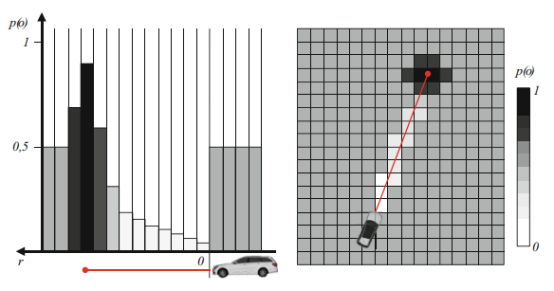
OGM updates the posterior occupancy probability following the Bayesian filtering mechanism. Given measurements at time from sensor inverse model, the binary state of each grid at time is estimated via a binary Bayesian filter(BBF)[175]:
| (8) | ||||
| (9) |
where and denote the probability of the occupied or free state, respectively.The preconditions for the establishment of Eqn. 8 include: the prior probabilities of occupancy state and free state are equal, measurements of grids are independent of each other, and the state does not change with time.
OGM has the following advantages: (a) a unified probabilistic form for environment perception with a solid theoretical foundation; (b) the ability to model complex obstacles of arbitrary shapes; (c) An intuitive and clear estimation of free space (driveable space); (d) A convenient framework for the fusion of different sensor data.
However, fixed-resolution OGM has obvious shortcomings which hinder its application in the field of autonomous driving. (a) Reasonable resolution for balancing precision and computation burden. (b) Sparse and noisy laser input leads to a large number of unknown regions[182]. An important premise for Eqn. 8 is that the measurement of the grid is completely independent, that is to say, when there is no radar ray reflection point in a grid, it will be regarded as an unknown state. The sparsity of the point cloud means that most of the grids in the environment are in unknown states. (c) Failure of static OGM to cope with dynamic scenes. Moving vehicles leave trails on static OGM.
-A2 Continuous Occupancy Map
The Continuous occupancy map is a split-new approach that uses continuous occupancy probability kernels which allows arbitrary resolutions of occupancy. A continuous occupancy map first divides the point cloud into free or occupied parts and updates the parameters in the kernel function according to these points or segments with known states, then using the obtained kernel function to estimate the occupancy state of any nearby location and realize the continuous occupation rate estimation of the whole space. Gaussian process occupancy maps (GPOMs)[183] use a modified Gaussian process classifier model as a non-parametric Bayesian technique while introducing correlations between points in the map to model the continuous probability representations of occupancy estimation with correlated variance maps in the real-world environment, especially those areas with sparse point clouds. But its time complexity is in the number of training points, which brings difficulties for real-time applications. Hilbert maps[130] project the original data into the Hilbert feature space based on the kernel feature approximation and use stochastic gradient descent to train a logistic regression classifier. This algorithm is robust to outliers and the update time is linear with the growth of data points, obtaining a favorable balance between the continuous occupancy estimation effect and real-time performance, but it cannot calculate the uncertainty of the estimation result like GPOM.
-A3 Dynamic Occupancy Map
In traffic scenarios, occupancy maps need to represent the occupancy of dynamic obstacles such as pedestrians and other vehicles and simultaneously estimate their motion state to further predict future trajectories and avoid driving risks.
The most intuitive method is to combine static grid map with multi-target tracking technology, which uses OGM to represent static obstacles and detection and tracking of moving objects (DATMO) to model dynamic obstacles. Early approaches obtain the range of dynamic obstacles by checking conflicts between grid map and the added observations and these conflicting regions would be used as input to the multi-target tracking algorithm and removed from the static grid map accordingly, yielding a robust static occupied raster map[184, 185, 186, 187, 188]. But the main issue with adopting two different environmental representations to model a unified scenario is the difficulty of data association. The static grid structure and the polygon list of dynamic obstacles are likely to be inconsistent when correlating. Meanwhile, the shape assumptions of dynamic obstacles limit the estimation accuracy and application range of the system, which is contrary to the advantage of OGM to represent arbitrary obstacles intuitively. Attempts on the data association issue include clustering conflicting grids and associating them directly to multi-object tracking to implement separate tracking of each part[189], and constructing exclusive local grid maps for each dynamic object[184].
Another key concern of the DATMO-based approach for representing dynamic objects is that both the detection and shape models of dynamic obstacles must be well trained[178], since the false and missed detections generated at this stage will propagate with the whole system process in a chain, leading that unknown objects and features in practical applications are probably to cause a significant impact on the performance of the algorithm. Therefore, a more reasonable approach is to directly improve the occupancy map itself in order to achieve a uniform and consistent representation of dynamic and static objects.
Dynamic Occupancy Grid Map (DOGM) integrates dynamic targets into the grid map and estimates the occupancy probability of obstacles corresponding to the grid as well as their velocity state, so as to improve the perception and obstacle avoidance capability of robots or autonomous vehicles for complex dynamic environments.
The methods are varied in the publications. For continuous occupancy maps, some have applied the dynamic obstacle assumption to existing static occupancy graph structures. For example, [190] used an optical flow-based motion map to estimate the velocity of the grid and improved the GPOM[183] to accommodate a dynamic environment. In [191], point clouds in LiDAR are clustered and filtered to estimate the velocity of dynamic obstacles, which is used to generate a non-stationary kernel in Hilbert space to build a dynamic Hilbert map[130].
Bayesian Occupancy Filter (BOF)[192, 193] is entirely grid-based with no object assumptions. BOF estimates the two-dimensional environment using a four-dimensional grid, where two grid dimensions represent the spatial position and two grid dimensions represent the two-dimensional velocity of the obstacle. Thus, BOF estimates the motion of an object and considers it explicitly in its process model. It uses the histogram of each grid to estimate the discrete grid velocity distribution, which means the velocity is equal to an exact integer grid displacement in the prediction process[193]. However, this discretization of the velocity leads to artifacts and limits the accuracy. In addition, each grid requires summing over all possible antecedent grids and their velocities, which is computationally expensive, especially when the environment needs to be expressed with high accuracy.
One class of methods that have emerged in recent years uses particles as the basis for maps, which were designed for dynamic environments from the beginning. In particle-based methods, obstacles are considered as a set of point objects and particles with velocity are used to simulate point objects. The theoretical basis of the particle-based approach originates from the Sequential Monte Carlo (SMC) filter[194, 195]. The entire dynamic grid is represented by a particle swarm, in which each particle represents an individual hypothesis that can move from one grid to another. Particle states are defined by position and velocity and are predicted across the grid based on their motion model and parameters. The article is directly associated with a grid based on its position, thus contributing to the occupancy and velocity distribution of this grid. The occupancy probability is described by the number of particles in the grid.
Random Finite Set (RFS) theory is introduced in [196] to particle-based maps and derived a map construction procedure using Probability Hypothesis Density (PHD) filters and Bernoulli filters. Dempster-Sheffer (DS) evidence theory is then used to update the occupancy state of a dynamic grid to significantly reduce the computational effort.
In cluttered environments with both dynamic and static obstacles, it is necessary to model dynamic or static multi-point objects and non-negligible noise may occur. To reduce the noise, two approaches are usually used. The first approach is to use a hybrid model [197, 198, 199], which includes a separate static model and a dynamic model to update the states of static and dynamic point objects independently. This hybrid model can be used as a dual PHD filter[197] or grid-level inference[198, 199]. Another approach is to apply additional information during the update to reduce noise, including object height[200], grayscale intensity[200, 201], semantic information[201] and object id[202, 203].
In conclusion, the existing particle-based DOGM are promising, but they have two limitations. The first limitation is that most solutions use the totality of a particle (a multi-modal probability density) to estimate the state of multiple grids that are considered independent (a grid is described by its own probability density). A particle can migrate from one grid to another, decoupled from its previous source grid density, and reassigned to a new target grid density. Because particles are recombined into new independent grid estimators in each iteration, the identity of the tracked grid is lost. However, if additional heuristics are used, this information can be retained. In other words, particles can usually identify the presence of an object, but not the presence of a ”specific” object part or grid. In order to improve estimation and data association, the authors of [202, 203] adopted the idea of connecting particles to objects by extending them with object ids. It should be noted that the proposed approach still ignores grid identification and must remap each particle to each grid.
The second limitation is that the estimation of grids belonging to large and homogeneous grid regions usually has high uncertainty and low accuracy. For example, a particle that is predicted to be in the middle of a larger object can attach to any of its occupied grids. This can lead to ambiguous data correlations and ultimately higher uncertainty. To improve the estimation accuracy in uniform grid regions (i.e., in the middle of large objects with the same occupancy values), additional features from different sensors, larger patches, or more particles are needed.
-B Camera-based Grid Mapping
As cameras provide information rich in semantic cues but lossy in geometric cues. Early researchers conduct 3D vision tasks on the perspective view (PV), which lacks enough geometry guidance. In recent years, vision BEV-based approaches achieve great success as BEV provides a structured coordinate encoding for pixel features from multi-view cameras. View projection from perspective view (PV) to bird’s eye view (BEV) is a major issue for vision-centric grid perception.
-B1 Geometry-based Transformation
Geometry-based methods utilize the natural geometric projection relationship between PV and BEV for transformation. These methods can be further divided into two categories: homograph-based and depth-based. Homograph-based methods are efficient for learning road surface layouts for autonomous driving, due to their hard flat-ground assumption. Depth-based methods are more common in representing obstacles on the road and achieving state-of-the-art performance.
Homograph-based methods. Inverse Perspective Mapping (IPM)[204] is the earliest and the most important work which uses a homography matrix to formulate the transformation under the constraint that the corresponding points lie on a horizontal plane. The homography matrix can be mathematically derived from intrinsic and extrinsic parameters of the camera. In addition to image projection, Cam2BEV[205], 3D-LaneNet[206] use IPM to transform feature maps for downstream perception tasks. Gu et al.[207] propose a Homography Loss for the training of the network. To reduce the distortion of the part above the ground plane caused by IPM, OGMs[208], SHOT[209] use semantic information and MonoLayout[210] utilizes Generative Adversarial Network (GAN)[211] to improve BEV features.
Depth-based methods. These methods rely heavily on voxels, an explicit 3D representation compatible with the end-to-end design. As shown in Fig. 20, depth-based methods use the predicted depth distribution per grid to lift 2D features to 3D voxel space and then generate the BEV 2D grid representation. This lift process writes:
| (10) |
where is pixel coordinate corresponding to in 3D space, is feature, is predicted depth distribution, * denotes one or more images, denotes outer production.
Depth is commonly formulated as a distribution. OFT[212], M2BEV[137] assume uniform depth distribution, which means that all 3D features along a ray are the same. Some other depth-based methods[213, 214, 107, 135, 215, 216] model the depth distribution with different learnable network structures and parameters.
Depth-based methods are usually supervised by labels from downstream tasks, but per-pixel depth supervision can also improve accuracy of depth estimation. CaDDN[213], DfM[214], BEVDepth[135] and STS[215] can optionally use depth supervision from LiDAR point clouds during the training stage.
Some structures are able to capture stereo cues in ring-camera settings. MV-FCOS3D++[216] uses pre-trained 2D feature extractors for a few stereo cues. BEVDepth proposes a depth correction module to solve the spatial misalignment between the image feature map and the ground truth derived from LiDAR caused by the ego vehicle’s motion. Combined with the monocular depth module in BEVDepth, BEVStereo[215] uses the geometrical correspondence between temporal dynamic stereo cameras to promote depth learning.
Depth-based methods are still dominant in vision-centric perception. Recent works such as FIERY[29], M2BEV[137], StretchBEV[95] and BEVerse[96] are based on BEV representation derived from depth-based LSS[107].
Fisheye BEV algorithm. Compared to pinhole cameras, fisheye cameras have a broader field of view and higher distortion. Most fisheye detection algorithms are based on the perspective view. Wu et al.[217] propose a surround-view fisheye dataset FPD and BEV-perception multi-task model, FPNet. It has a shared feature extractor as well as 2D and 3D detection heads and per-pixel depth head.
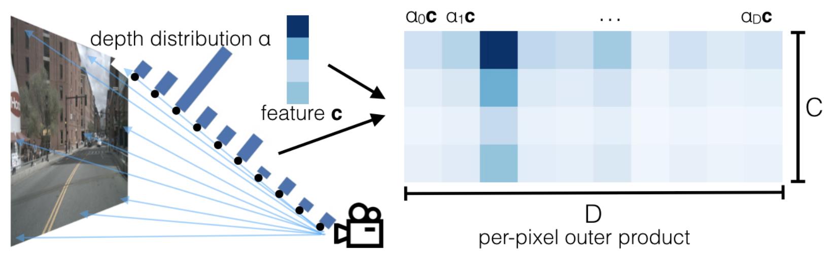
-B2 Network-based Transformation
Network-based transformation methods utilize deep neural networks as a mapping function to model the view transformation and use the camera geometry implicitly. Recent methods can also be further divided into two categories: MLP-based and transformer-based. The former conducts the transformation in a forward way, while the latter constructs BEV queries and searches for corresponding features on PV maps through a cross-attention mechanism.
MLP-based methods. Multi-layer perceptron is employed to model the transformation from PV to BEV without camera parameters. Therefore, they avoid inductive biases from the calibrated camera system. VED[219] utilizes a variational encoder-decoder MLP network to predict BEV semantic occupancy grid map from a front-view monocular image in real-time. To use the information from different views to achieve surrounding sensing, VPN[220] designs a view transformer module (VTM) with two-layer MLP to fuse each PV feature map into a BEV feature map. FishingNet[62] transforms the camera features to BEV maps by modifying the VTM, and then fuse them with radar and LiDAR data for multi-modal perception and prediction. To predict more accurate BEV maps from monocular images, PON[221] and STA-ST[222] include a feature pyramid network(FPN)[223] to provide high-resolution features with rich context. The dense transformer layer in PON collapses PV features along height axis and expands them along the depth axis through MLP before resampling them to obtain BEV features in Cartesian coordinates. HDMapNet[87] puts forward a novel view transformer module that consists of MLP-based neural feature transformation and geometric projection. It can produce a vectorized local semantic map from images of the surrounding cameras. Since the projection of BEV features back to the PV map can form self-supervision, PYVA[224] includes a cross-view transformation module that utilizes an MLP-based cycle to retain the features related to view transformation. To reap the benefits of homograph-based methods and MLP-based methods, HFT[225] consists of two branches to utilize geometric priors and global context respectively.
MLP-based methods tend to transform multi-view images individually and ignore the geometric potential brought by overlapping regions. These shortcomings make its application less widespread than subsequent transformer-based methods.
Transformer-based methods. Vaswani et al.[226] introduce transformer, an attention-based model which facilitates the development of natural language processing (NLP). Vision transformers have shown remarkable performance in various vision tasks due to its ability to capture long-range dependencies and global receptive fields. Compared to MLP-based methods, transformer-based methods view transformation have more impressive PV2BEV relation modeling ability. Query-based element extraction starts with 2D object detector DETR[227].
To satisfy the requirements of grid-centric perception tasks, the granularity of the query in the transformer decoder should be finer and each query is position-encoded according to its spatial location in 3D space or BEV space. Tesla[228] first conducts the view transformation through cross-attention between dense BEV queries and multi-view image features. CVT[229] points out that geometric reasoning of cross-attention transformers performs well and inferences faster than geometric models. So it employs cross-view transformers for view transformation, which use positional embeddings derived from calibrated camera intrinsics and extrinsics. In addition to an MLP-based cycled view projection mentioned above, PYVA’s[224] transformation module also contains a cross-view transformer to correlate the features before and after view projection.
To avoid high computation complexity in the transformer attention module, one approach is to use sparse attention. Deformable attention[230] reduces the number of keys to avoid excessive attention computation by only focusing on relevant regions and capturing informative features. The view transformation module of many works use this sparse attention, such as BEVSegFormer[231] shown in Fig. 21, PersFormer[232] and BEVFormer[89]. Note that the queries in BEVSegFormer directly predict the reference points on images, while PersFormer and BEVFormer rely on camera parameters to compute the reference points. Apart from deformable attention, several kinds of sparse attention are put forward. GKT[134] unfolds kernel regions around the projected reference points and makes them interact with dense BEV queries to generate BEV representation. ViT-BEVSeg[233] uses simpler and plain vision transformer for patch embedding-based view transformation.
Another approach is to simplify the cross-attention computation with 3D geometry constraints. Image2Map[234] uses camera geometry to dictate one-to-one correspondence between vertical scan lines in the image and polar rays in the BEV map to form an inter-plane attention mechanism. The view transformation is treated as a set of sequence-to-sequence translations. Similarly, PolarFormer[235] also employs this correspondence to simplify the global attention into column-wise attention and uses a polar alignment module to aggregate rays from multiple camera views to generate a structured Polar BEV feature map.
PETRv2[236] is developed from PETR[237] which contains sparse object queries for object-centric tasks. In order to form a unified framework for 3D perception, PETRv2 adds a set of BEV segmentation queries to support high-quality BEV segmentation, an important grid-centric task.
Geometric cues and temporal cues are both important to transformer-based methods. As geometric cues, calibrated camera parameters are utilized in many transformer-based methods to reduce memory/computation complexity or improve data efficiency. As mentioned above, [229, 236] generate 3D positional embedding derived from camera parameters to help the transformers learn view transformation. [232, 89, 134] rely on camera parameters to compute the reference points for feature sampling. [234, 235] employs camera geometry to dictate the relationship between each vertical scanline in the image and the BEV features. However, with such geometric cues it is possible to introduce inductive biases contained in the calibrated camera system. Temporal cues which are used in [89, 235] can improve the performance of methods.
Polar coordinate. Common practices adopt Cartesian coordinate with evenly distributed rectangular grids. However, PolarBEV[238] argues that surrounding grids should be paid more attention than distant ones, so unevenly distributed polar rasterization can reduce computational budget. PolarDETR[239] models multi-view BEV detection transformer on Polar parameterizations. PolarFormer[235] extracts dense BEV features on polar coordinates and surpasses Cartesian coordinate counterparts in BEVFormer[89].
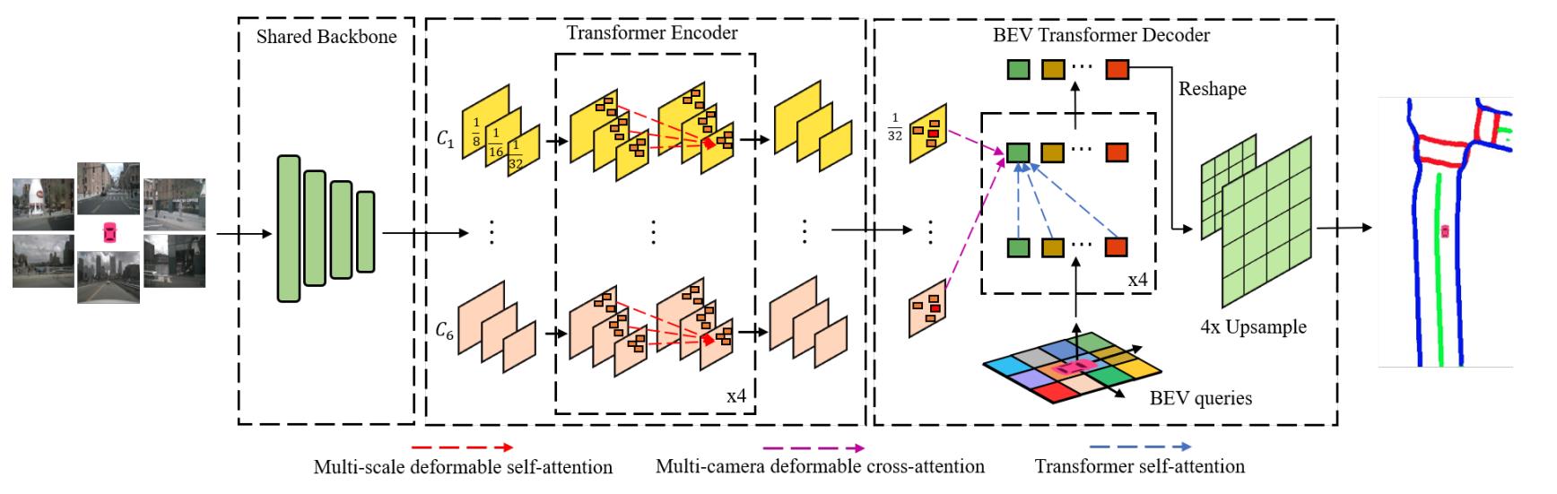
References
- [1] J. Mao, S. Shi, X. Wang, and H. Li, “3d object detection for autonomous driving: a review and new outlooks,” arXiv preprint arXiv:2206.09474, 2022.
- [2] R. Qian, X. Lai, and X. Li, “3D Object Detection for Autonomous Driving: A Survey,” Pattern Recognition, vol. 130, no. 8, pp. 1–24, 2022.
- [3] K. Gao, Y. Gao, H. He, D. Lu, L. Xu, and J. Li, “NeRF: Neural Radiance Field in 3D Vision, A Comprehensive Review,” pp. 1–20, 2022. [Online]. Available: http://arxiv.org/abs/2210.00379
- [4] Y. Ma, T. Wang, X. Bai, H. Yang, Y. Hou, Y. Wang, Y. Qiao, R. Yang, D. Manocha, and X. Zhu, “Vision-centric bev perception: A survey,” arXiv preprint arXiv:2208.02797, 2022.
- [5] H. Li, C. Sima, J. Dai, W. Wang, L. Lu, H. Wang, E. Xie, Z. Li, H. Deng, H. Tian, et al., “Delving into the devils of bird’s-eye-view perception: A review, evaluation and recipe,” arXiv preprint arXiv:2209.05324, 2022.
- [6] A. Fisher, R. Cannizzaro, M. Cochrane, C. Nagahawatte, and J. L. Palmer, “Colmap: A memory-efficient occupancy grid mapping framework,” Robotics and Autonomous Systems, vol. 142, p. 103755, 2021.
- [7] R. Barrett and S. J. Delany, “Openmvc: a non-proprietry component-based framework for web applications,” in Proceedings of the 13th international World Wide Web conference on Alternate track papers & posters, 2004, pp. 464–465.
- [8] B. Mildenhall, P. P. Srinivasan, M. Tancik, J. T. Barron, R. Ramamoorthi, and R. Ng, “NeRF: Representing Scenes as Neural Radiance Fields for View Synthesis,” Lecture Notes in Computer Science (including subseries Lecture Notes in Artificial Intelligence and Lecture Notes in Bioinformatics), vol. 12346 LNCS, pp. 405–421, 2020.
- [9] A.-Q. Cao and R. de Charette, “Monoscene: Monocular 3d semantic scene completion,” in Proceedings of the IEEE/CVF Conference on Computer Vision and Pattern Recognition, 2022, pp. 3991–4001.
- [10] M. Schreiber, V. Belagiannis, C. Gläser, and K. Dietmayer, “A Multi-Task Recurrent Neural Network for End-to-End Dynamic Occupancy Grid Mapping,” 2022. [Online]. Available: http://arxiv.org/abs/2202.04461
- [11] K. Mani, N. Sai Shankar, K. Murthy Jatavallabhula, and K. Madhava Krishna, “AutoLay: Benchmarking amodal layout estimation for autonomous driving,” IEEE International Conference on Intelligent Robots and Systems, pp. 8184–8191, 2020.
- [12] P. Wu, S. Chen, and D. N. Metaxas, “MotionNet: Joint Perception and Motion Prediction for Autonomous Driving Based on Bird’s Eye View Maps,” Proceedings of the IEEE Computer Society Conference on Computer Vision and Pattern Recognition, pp. 11 382–11 392, 2020.
- [13] L. Zheng, Z. Ma, X. Zhu, B. Tan, S. Li, K. Long, W. Sun, S. Chen, L. Zhang, M. Wan, et al., “Tj4dradset: A 4d radar dataset for autonomous driving,” arXiv preprint arXiv:2204.13483, 2022.
- [14] M. Meyer and G. Kuschk, “Automotive radar dataset for deep learning based 3d object detection,” in 2019 16th european radar conference (EuRAD). IEEE, 2019, pp. 129–132.
- [15] J. Cen, P. Yun, J. Cai, M. Y. Wang, and M. Liu, “Open-set 3d object detection,” in 2021 International Conference on 3D Vision (3DV). IEEE, 2021, pp. 869–878.
- [16] K. Joseph, S. Khan, F. S. Khan, and V. N. Balasubramanian, “Towards open world object detection,” in Proceedings of the IEEE/CVF Conference on Computer Vision and Pattern Recognition, 2021, pp. 5830–5840.
- [17] A. Gupta, S. Narayan, K. Joseph, S. Khan, F. S. Khan, and M. Shah, “Ow-detr: Open-world detection transformer,” in Proceedings of the IEEE/CVF Conference on Computer Vision and Pattern Recognition, 2022, pp. 9235–9244.
- [18] O. Zohar, K.-C. Wang, and S. Yeung, “PROB: Probabilistic Objectness for Open World Object Detection,” pp. 31–33, 2022. [Online]. Available: http://arxiv.org/abs/2212.01424
- [19] A. Hornung, K. M. Wurm, M. Bennewitz, C. Stachniss, and W. Burgard, “Octomap: An efficient probabilistic 3d mapping framework based on octrees,” Autonomous robots, vol. 34, no. 3, pp. 189–206, 2013.
- [20] J. Behley, M. Garbade, A. Milioto, J. Quenzel, S. Behnke, C. Stachniss, and J. Gall, “Semantickitti: A dataset for semantic scene understanding of lidar sequences,” in 2019 IEEE/CVF International Conference on Computer Vision (ICCV), 2019, pp. 9296–9306.
- [21] A. Geiger, P. Lenz, and R. Urtasun, “Are we ready for autonomous driving? the kitti vision benchmark suite,” in 2012 IEEE Conference on Computer Vision and Pattern Recognition, 2012, pp. 3354–3361.
- [22] R. Kesten, M. Usman, J. Houston, T. Pandya, K. Nadhamuni, A. Ferreira, M. Yuan, B. Low, A. Jain, P. Ondruska, S. Omari, S. Shah, A. Kulkarni, A. Kazakova, C. Tao, L. Platinsky, W. Jiang, and V. Shet, “Level 5 perception dataset 2020,” https://level-5.global/level5/data/, 2019.
- [23] M.-F. Chang, J. Lambert, P. Sangkloy, J. Singh, S. Bak, A. Hartnett, D. Wang, P. Carr, S. Lucey, D. Ramanan, and J. Hays, “Argoverse: 3d tracking and forecasting with rich maps,” in 2019 IEEE/CVF Conference on Computer Vision and Pattern Recognition (CVPR), 2019, pp. 8740–8749.
- [24] H. Caesar, V. Bankiti, A. H. Lang, S. Vora, V. E. Liong, Q. Xu, A. Krishnan, Y. Pan, G. Baldan, and O. Beijbom, “nuscenes: A multimodal dataset for autonomous driving,” in 2020 IEEE/CVF Conference on Computer Vision and Pattern Recognition (CVPR), 2020, pp. 11 618–11 628.
- [25] P. Sun, H. Kretzschmar, X. Dotiwalla, A. Chouard, V. Patnaik, P. Tsui, J. Guo, Y. Zhou, Y. Chai, B. Caine, V. Vasudevan, W. Han, J. Ngiam, H. Zhao, A. Timofeev, S. Ettinger, M. Krivokon, A. Gao, A. Joshi, Y. Zhang, J. Shlens, Z. Chen, and D. Anguelov, “Scalability in perception for autonomous driving: Waymo open dataset,” in 2020 IEEE/CVF Conference on Computer Vision and Pattern Recognition (CVPR), 2020, pp. 2443–2451.
- [26] Y. Liao, J. Xie, and A. Geiger, “Kitti-360: A novel dataset and benchmarks for urban scene understanding in 2d and 3d,” IEEE Transactions on Pattern Analysis and Machine Intelligence, pp. 1–1, 2022.
- [27] B. Wilson, W. Qi, T. Agarwal, J. Lambert, J. Singh, S. Khandelwal, B. Pan, R. Kumar, A. Hartnett, J. K. Pontes, D. Ramanan, and J. Hays, “Argoverse 2: Next generation datasets for self-driving perception and forecasting,” in NeurIPS Datasets and Benchmarks, 2021.
- [28] J. Mao, M. Niu, C. Jiang, X. Liang, Y. Li, C. Ye, W. Zhang, Z. Li, J. Yu, C. Xu, et al., “One million scenes for autonomous driving: Once dataset,” 2021.
- [29] A. Hu, Z. Murez, N. Mohan, S. Dudas, J. Hawke, V. Badrinarayanan, R. Cipolla, and A. Kendall, “FIERY: Future Instance Prediction in Bird’s-Eye View from Surround Monocular Cameras,” Proceedings of the IEEE International Conference on Computer Vision, pp. 15 253–15 262, 2021.
- [30] D. Kim, S. Woo, J.-Y. Lee, and I. S. Kweon, “Video panoptic segmentation,” in 2020 IEEE/CVF Conference on Computer Vision and Pattern Recognition (CVPR), 2020, pp. 9856–9865.
- [31] G. Máttyus, W. Luo, and R. Urtasun, “Deeproadmapper: Extracting road topology from aerial images,” in 2017 IEEE International Conference on Computer Vision (ICCV), 2017, pp. 3458–3466.
- [32] S. Shi, X. Wang, and H. Li, “Pointrcnn: 3d object proposal generation and detection from point cloud,” in Proceedings of the IEEE/CVF conference on computer vision and pattern recognition, 2019, pp. 770–779.
- [33] S. Shi, C. Guo, L. Jiang, Z. Wang, J. Shi, X. Wang, and H. Li, “Pv-rcnn: Point-voxel feature set abstraction for 3d object detection,” in Proceedings of the IEEE/CVF Conference on Computer Vision and Pattern Recognition, 2020, pp. 10 529–10 538.
- [34] X. Chen, H. Ma, J. Wan, B. Li, and T. Xia, “Multi-view 3d object detection network for autonomous driving,” in Proceedings of the IEEE conference on Computer Vision and Pattern Recognition, 2017, pp. 1907–1915.
- [35] J. Ku, M. Mozifian, J. Lee, A. Harakeh, and S. L. Waslander, “Joint 3d proposal generation and object detection from view aggregation,” in 2018 IEEE/RSJ International Conference on Intelligent Robots and Systems (IROS). IEEE, 2018, pp. 1–8.
- [36] B. Yang, W. Luo, and R. Urtasun, “Pixor: Real-time 3d object detection from point clouds,” in Proceedings of the IEEE conference on Computer Vision and Pattern Recognition, 2018, pp. 7652–7660.
- [37] S. Mohapatra, S. Yogamani, H. Gotzig, S. Milz, and P. Mader, “Bevdetnet: bird’s eye view lidar point cloud based real-time 3d object detection for autonomous driving,” in 2021 IEEE International Intelligent Transportation Systems Conference (ITSC). IEEE, 2021, pp. 2809–2815.
- [38] Y. Zhou and O. Tuzel, “Voxelnet: End-to-end learning for point cloud based 3d object detection,” in Proceedings of the IEEE conference on computer vision and pattern recognition, 2018, pp. 4490–4499.
- [39] A. H. Lang, S. Vora, H. Caesar, L. Zhou, J. Yang, and O. Beijbom, “Pointpillars: Fast encoders for object detection from point clouds,” in Proceedings of the IEEE/CVF conference on computer vision and pattern recognition, 2019, pp. 12 697–12 705.
- [40] S. Li, T. Wang, S. Yang, and Y. Yuan, “Efficientpillarnet: A fast deep network for semantic segmentation of large-scale point clouds from lidar,” in 2021 International Conference of Optical Imaging and Measurement (ICOIM). IEEE, 2021, pp. 295–300.
- [41] G. Shi, R. Li, and C. Ma, “Pillarnet: High-performance pillar-based 3d object detection,” arXiv preprint arXiv:2205.07403, 2022.
- [42] J. Wilson, J. Song, Y. Fu, A. Zhang, A. Capodieci, P. Jayakumar, K. Barton, and M. Ghaffari, “Motionsc: Data set and network for real-time semantic mapping in dynamic environments,” IEEE Robotics and Automation Letters, vol. 7, no. 3, pp. 8439–8446, 2022.
- [43] Y. H. Khalil and H. T. Mouftah, “Licanet: Further enhancement of joint perception and motion prediction based on multi-modal fusion,” IEEE Open Journal of Intelligent Transportation Systems, vol. 3, pp. 222–235, 2022.
- [44] ——, “Licanext: Incorporating sequential range residuals for additional advancement in joint perception and motion prediction,” IEEE Access, vol. 9, pp. 146 244–146 255, 2021.
- [45] Y. Li, Y. Chen, X. Qi, Z. Li, J. Sun, and J. Jia, “Unifying voxel-based representation with transformer for 3d object detection,” arXiv preprint arXiv:2206.00630, 2022.
- [46] Z. Chen, Z. Li, S. Zhang, L. Fang, Q. Jiang, F. Zhao, B. Zhou, and H. Zhao, “Autoalign: Pixel-instance feature aggregation for multi-modal 3d object detection,” arXiv preprint arXiv:2201.06493, 2022.
- [47] Z. Chen, Z. Li, S. Zhang, L. Fang, Q. Jiang, and F. Zhao, “Autoalignv2: Deformable feature aggregation for dynamic multi-modal 3d object detection,” arXiv preprint arXiv:2207.10316, 2022.
- [48] X. Chen, T. Zhang, Y. Wang, Y. Wang, and H. Zhao, “Futr3d: A unified sensor fusion framework for 3d detection,” arXiv preprint arXiv:2203.10642, 2022.
- [49] X. Bai, Z. Hu, X. Zhu, Q. Huang, Y. Chen, H. Fu, and C.-L. Tai, “Transfusion: Robust lidar-camera fusion for 3d object detection with transformers,” in Proceedings of the IEEE/CVF Conference on Computer Vision and Pattern Recognition, 2022, pp. 1090–1099.
- [50] Z. Liu, H. Tang, A. Amini, X. Yang, H. Mao, D. Rus, and S. Han, “Bevfusion: Multi-task multi-sensor fusion with unified bird’s-eye view representation,” arXiv preprint arXiv:2205.13542, 2022.
- [51] T. Liang, H. Xie, K. Yu, Z. Xia, Z. Lin, Y. Wang, T. Tang, B. Wang, and Z. Tang, “Bevfusion: A simple and robust lidar-camera fusion framework,” arXiv preprint arXiv:2205.13790, 2022.
- [52] Z. Yang, J. Chen, Z. Miao, W. Li, X. Zhu, and L. Zhang, “Deepinteraction: 3d object detection via modality interaction,” arXiv preprint arXiv:2208.11112, 2022.
- [53] Y. Jiao, Z. Jie, S. Chen, J. Chen, X. Wei, L. Ma, and Y.-G. Jiang, “Msmdfusion: Fusing lidar and camera at multiple scales with multi-depth seeds for 3d object detection,” arXiv preprint arXiv:2209.03102, 2022.
- [54] L. Sless, B. E. Shlomo, G. Cohen, and S. Oron, “Road scene understanding by occupancy grid learning from sparse radar clusters using semantic segmentation,” in 2019 IEEE/CVF International Conference on Computer Vision Workshop (ICCVW), 2019, pp. 867–875.
- [55] A. Popov, P. Gebhardt, K. Chen, R. Oldja, H. Lee, S. Murray, R. Bhargava, and N. Smolyanskiy, “NVRadarNet: Real-Time Radar Obstacle and Free Space Detection for Autonomous Driving,” 2022. [Online]. Available: http://arxiv.org/abs/2209.14499
- [56] A. W. Harley, Z. Fang, J. Li, R. Ambrus, and K. Fragkiadaki, “Simple-BEV: What really matters for multi-sensor bev perception?” in arXiv:2206.07959, 2022.
- [57] T. Zhou, J. Chen, Y. Shi, K. Jiang, M. Yang, and D. Yang, “Bridging the view disparity between radar and camera features for multi-modal fusion 3d object detection,” IEEE Transactions on Intelligent Vehicles, pp. 1–14, 2023.
- [58] J.-J. Hwang, H. Kretzschmar, J. Manela, S. Rafferty, N. Armstrong-Crews, T. Chen, and D. Anguelov, “CramNet: Camera-Radar Fusion with Ray-Constrained Cross-Attention for Robust 3D Object Detection,” no. Figure 1, pp. 388–405, 2022.
- [59] C. R. Qi, L. Yi, H. Su, and L. J. Guibas, “Pointnet++: Deep hierarchical feature learning on point sets in a metric space,” arXiv preprint arXiv:1706.02413, 2017.
- [60] A. W. Harley, Z. Fang, J. Li, R. Ambrus, and K. Fragkiadaki, “A simple baseline for bev perception without lidar,” arXiv preprint arXiv:2206.07959, 2022.
- [61] Y. Yang, J. Liu, T. Huang, Q.-L. Han, G. Ma, and B. Zhu, “RaLiBEV: Radar and LiDAR BEV Fusion Learning for Anchor Box Free Object Detection System,” pp. 1–12, 2022. [Online]. Available: http://arxiv.org/abs/2211.06108
- [62] N. Hendy, C. Sloan, F. Tian, P. Duan, N. Charchut, Y. Xie, C. Wang, and J. Philbin, “Fishing net: Future inference of semantic heatmaps in grids,” arXiv preprint arXiv:2006.09917, 2020.
- [63] R. Xu, Z. Tu, H. Xiang, W. Shao, B. Zhou, and J. Ma, “Cobevt: Cooperative bird’s eye view semantic segmentation with sparse transformers,” arXiv preprint arXiv:2207.02202, 2022.
- [64] H. Li and F. Nashashibi, “A new method for occupancy grid maps merging: Application to multi-vehicle cooperative local mapping and moving object detection in outdoor environment,” in 2012 12th International Conference on Control Automation Robotics & Vision (ICARCV). IEEE, 2012, pp. 632–637.
- [65] X. Zheng, Y. Li, D. Duan, L. Yang, C. Chen, and X. Cheng, “Multi-vehicle multi-sensor occupancy grid maps (mvms-ogm) for autonomous driving,” IEEE Internet of Things Journal, 2022.
- [66] Y. Yuan, H. Cheng, M. Y. Yang, and M. Sester, “Generating evidential bev maps in continuous driving space,” arXiv preprint arXiv:2302.02928, 2023.
- [67] L. Roldão, R. de Charette, and A. Verroust-Blondet, “Lmscnet: Lightweight multiscale 3d semantic completion,” in 2020 International Conference on 3D Vision (3DV), 2020, pp. 111–119.
- [68] S. Song, F. Yu, A. Zeng, A. X. Chang, M. Savva, and T. Funkhouser, “Semantic scene completion from a single depth image,” in Proceedings of the IEEE conference on computer vision and pattern recognition, 2017, pp. 1746–1754.
- [69] M. Garbade, Y.-T. Chen, J. Sawatzky, and J. Gall, “Two stream 3d semantic scene completion,” in Proceedings of the IEEE/CVF Conference on Computer Vision and Pattern Recognition Workshops, 2019, pp. 0–0.
- [70] R. Cheng, C. Agia, Y. Ren, X. Li, and L. Bingbing, “S3cnet: A sparse semantic scene completion network for lidar point clouds,” arXiv preprint arXiv:2012.09242, 2020.
- [71] X. Yan, J. Gao, J. Li, R. Zhang, Z. Li, R. Huang, and S. Cui, “Sparse single sweep lidar point cloud segmentation via learning contextual shape priors from scene completion,” in Proceedings of the AAAI Conference on Artificial Intelligence, vol. 35, no. 4, 2021, pp. 3101–3109.
- [72] C. B. Rist, D. Emmerichs, M. Enzweiler, and D. M. Gavrila, “Semantic scene completion using local deep implicit functions on lidar data,” IEEE Transactions on Pattern Analysis and Machine Intelligence, vol. 44, no. 10, pp. 7205–7218, 2022.
- [73] Y. Huang, W. Zheng, Y. Zhang, J. Zhou, and J. Lu, “Tri-perspective view for vision-based 3d semantic occupancy prediction,” 2023. [Online]. Available: https://arxiv.org/abs/2302.07817
- [74] Y. Li, Z. Yu, C. Choy, C. Xiao, J. M. Alvarez, S. Fidler, C. Feng, and A. Anandkumar, “Voxformer: Sparse voxel transformer for camera-based 3d semantic scene completion,” 2023. [Online]. Available: https://arxiv.org/abs/2302.12251
- [75] R. Miao, W. Liu, M. Chen, Z. Gong, W. Xu, C. Hu, and S. Zhou, “Occdepth: A depth-aware method for 3d semantic scene completion,” 2023. [Online]. Available: https://arxiv.org/abs/2302.13540
- [76] L. Roldão, R. de Charette, and A. Verroust-Blondet, “3D Semantic Scene Completion: A Survey,” International Journal of Computer Vision, vol. 130, no. 8, pp. 1978–2005, 2022.
- [77] S. Liu, Y. Hu, Y. Zeng, Q. Tang, B. Jin, Y. Han, and X. Li, “See and think: Disentangling semantic scene completion,” Advances in Neural Information Processing Systems, vol. 31, 2018.
- [78] B. Graham, M. Engelcke, and L. Van Der Maaten, “3d semantic segmentation with submanifold sparse convolutional networks,” in Proceedings of the IEEE conference on computer vision and pattern recognition, 2018, pp. 9224–9232.
- [79] C. Choy, J. Gwak, and S. Savarese, “4d spatio-temporal convnets: Minkowski convolutional neural networks,” in Proceedings of the IEEE/CVF Conference on Computer Vision and Pattern Recognition, 2019, pp. 3075–3084.
- [80] A. Dosovitskiy, G. Ros, F. Codevilla, A. Lopez, and V. Koltun, “Carla: An open urban driving simulator,” in Conference on robot learning. PMLR, 2017, pp. 1–16.
- [81] K. Rematas, A. Liu, P. P. Srinivasan, J. T. Barron, A. Tagliasacchi, T. Funkhouser, and V. Ferrari, “Urban radiance fields,” in Proceedings of the IEEE/CVF Conference on Computer Vision and Pattern Recognition, 2022, pp. 12 932–12 942.
- [82] M. Tancik, V. Casser, X. Yan, S. Pradhan, B. Mildenhall, P. P. Srinivasan, J. T. Barron, and H. Kretzschmar, “Block-nerf: Scalable large scene neural view synthesis,” in Proceedings of the IEEE/CVF Conference on Computer Vision and Pattern Recognition, 2022, pp. 8248–8258.
- [83] A.-Q. Cao and R. de Charette, “Scenerf: Self-supervised monocular 3d scene reconstruction with radiance fields,” arXiv preprint arXiv:2212.02501, 2022.
- [84] F. Wimbauer, N. Yang, C. Rupprecht, and D. Cremers, “Behind the Scenes: Density Fields for Single View Reconstruction,” 2023. [Online]. Available: http://arxiv.org/abs/2301.07668
- [85] A. Carlson, M. S. Ramanagopal, N. Tseng, M. Johnson-Roberson, R. Vasudevan, and K. A. Skinner, “Cloner: Camera-lidar fusion for occupancy grid-aided neural representations,” arXiv preprint arXiv:2209.01194, 2022.
- [86] Y. B. Can, A. Liniger, D. P. Paudel, and L. Van Gool, “Structured Bird’s-Eye-View Traffic Scene Understanding from Onboard Images,” Proceedings of the IEEE International Conference on Computer Vision, no. Iccv, pp. 15 641–15 650, 2021.
- [87] Q. Li, Y. Wang, Y. Wang, and H. Zhao, “Hdmapnet: An online hd map construction and evaluation framework,” in 2022 International Conference on Robotics and Automation (ICRA). IEEE, 2022, pp. 4628–4634.
- [88] J. Huang and G. Huang, “Bevdet4d: Exploit temporal cues in multi-camera 3d object detection,” arXiv preprint arXiv:2203.17054, 2022.
- [89] Z. Li, W. Wang, H. Li, E. Xie, C. Sima, T. Lu, Y. Qiao, and J. Dai, “Bevformer: Learning bird’s-eye-view representation from multi-camera images via spatiotemporal transformers,” in Computer Vision–ECCV 2022: 17th European Conference, Tel Aviv, Israel, October 23–27, 2022, Proceedings, Part IX. Springer, 2022, pp. 1–18.
- [90] Z. Qin, J. Chen, C. Chen, X. Chen, and X. Li, “Uniformer: Unified multi-view fusion transformer for spatial-temporal representation in bird’s-eye-view,” arXiv preprint arXiv:2207.08536, 2022.
- [91] S. Rusinkiewicz and M. Levoy, “Efficient variants of the icp algorithm,” in Proceedings third international conference on 3-D digital imaging and modeling. IEEE, 2001, pp. 145–152.
- [92] P. Biber and W. Straßer, “The normal distributions transform: A new approach to laser scan matching,” in Proceedings 2003 IEEE/RSJ International Conference on Intelligent Robots and Systems (IROS 2003)(Cat. No. 03CH37453), vol. 3. IEEE, 2003, pp. 2743–2748.
- [93] C. Luo, X. Yang, and A. Yuille, “Self-Supervised Pillar Motion Learning for Autonomous Driving,” Proceedings of the IEEE Computer Society Conference on Computer Vision and Pattern Recognition, pp. 3182–3191, 2021.
- [94] Y. Wang, H. Pan, J. Zhu, Y.-H. Wu, X. Zhan, K. Jiang, and D. Yang, “Be-sti: Spatial-temporal integrated network for class-agnostic motion prediction with bidirectional enhancement,” in Proceedings of the IEEE/CVF Conference on Computer Vision and Pattern Recognition, 2022, pp. 17 093–17 102.
- [95] A. K. Akan and F. Güney, “Stretchbev: Stretching future instance prediction spatially and temporally,” in Computer Vision–ECCV 2022: 17th European Conference, Tel Aviv, Israel, October 23–27, 2022, Proceedings, Part XXXVIII. Springer, 2022, pp. 444–460.
- [96] Y. Zhang, Z. Zhu, W. Zheng, J. Huang, G. Huang, J. Zhou, and J. Lu, “Beverse: Unified perception and prediction in birds-eye-view for vision-centric autonomous driving,” arXiv preprint arXiv:2205.09743, 2022.
- [97] S. Hu, L. Chen, P. Wu, H. Li, J. Yan, and D. Tao, “St-p3: End-to-end vision-based autonomous driving via spatial-temporal feature learning,” in Computer Vision–ECCV 2022: 17th European Conference, Tel Aviv, Israel, October 23–27, 2022, Proceedings, Part XXXVIII. Springer, 2022, pp. 533–549.
- [98] S. Targ, D. Almeida, and K. Lyman, “Resnet in resnet: Generalizing residual architectures,” arXiv preprint arXiv:1603.08029, 2016.
- [99] A. Jain, S. Casas, R. Liao, Y. Xiong, S. Feng, S. Segal, and R. Urtasun, “Discrete residual flow for probabilistic pedestrian behavior prediction,” in Conference on Robot Learning. PMLR, 2020, pp. 407–419.
- [100] M. Bansal, A. Krizhevsky, and A. S. Ogale, “Chauffeurnet: Learning to drive by imitating the best and synthesizing the worst,” CoRR, vol. abs/1812.03079, 2018. [Online]. Available: http://arxiv.org/abs/1812.03079
- [101] J. Hong, B. Sapp, and J. Philbin, “Rules of the road: Predicting driving behavior with a convolutional model of semantic interactions,” in Proceedings of the IEEE/CVF Conference on Computer Vision and Pattern Recognition, 2019, pp. 8454–8462.
- [102] S. Casas, A. Sadat, and R. Urtasun, “Mp3: A unified model to map, perceive, predict and plan,” in Proceedings of the IEEE/CVF Conference on Computer Vision and Pattern Recognition, 2021, pp. 14 403–14 412.
- [103] Y. Hu, W. Shao, B. Jiang, J. Chen, S. Chai, Z. Yang, J. Qian, H. Zhou, and Q. Liu, “Hope: Hierarchical spatial-temporal network for occupancy flow prediction,” arXiv preprint arXiv:2206.10118, 2022.
- [104] X. Huang, X. Tian, J. Gu, Q. Sun, and H. Zhao, “VectorFlow: Combining Images and Vectors for Traffic Occupancy and Flow Prediction,” pp. 2–5, 2022. [Online]. Available: http://arxiv.org/abs/2208.04530
- [105] H. Liu, Z. Huang, and C. Lv, “Strajnet: Occupancy flow prediction via multi-modal swin transformer,” arXiv preprint arXiv:2208.00394, 2022.
- [106] R. Cipolla, Y. Gal, and A. Kendall, “Multi-task learning using uncertainty to weigh losses for scene geometry and semantics,” in 2018 IEEE/CVF Conference on Computer Vision and Pattern Recognition, 2018, pp. 7482–7491.
- [107] J. Philion and S. Fidler, “Lift, Splat, Shoot: Encoding Images from Arbitrary Camera Rigs by Implicitly Unprojecting to 3D,” Lecture Notes in Computer Science (including subseries Lecture Notes in Artificial Intelligence and Lecture Notes in Bioinformatics), vol. 12359 LNCS, pp. 194–210, 2020.
- [108] C. Lu and G. Dubbelman, “Hallucinating beyond observation: Learning to complete with partial observation and unpaired prior knowledge,” arXiv preprint arXiv:1907.09786, 2019.
- [109] T. Yin, X. Zhou, and P. Krähenbühl, “Center-based 3d object detection and tracking,” in 2021 IEEE/CVF Conference on Computer Vision and Pattern Recognition (CVPR), 2021, pp. 11 779–11 788.
- [110] X. Zhu, W. Su, L. Lu, B. Li, X. Wang, and J. Dai, “Deformable DETR: deformable transformers for end-to-end object detection,” in 9th International Conference on Learning Representations, ICLR 2021, Virtual Event, Austria, May 3-7, 2021. OpenReview.net, 2021. [Online]. Available: https://openreview.net/forum?id=gZ9hCDWe6ke
- [111] E. Xie, W. Wang, Z. Yu, A. Anandkumar, J. M. Alvarez, and P. Luo, “Segformer: Simple and efficient design for semantic segmentation with transformers,” in Advances in Neural Information Processing Systems 34: Annual Conference on Neural Information Processing Systems 2021, NeurIPS 2021, December 6-14, 2021, virtual, M. Ranzato, A. Beygelzimer, Y. N. Dauphin, P. Liang, and J. W. Vaughan, Eds., 2021, pp. 12 077–12 090. [Online]. Available: https://proceedings.neurips.cc/paper/2021/hash/64f1f27bf1b4ec22924fd0acb550c235-Abstract.html
- [112] Z. Li, W. Wang, E. Xie, Z. Yu, A. Anandkumar, J. M. Álvarez, T. Lu, and P. Luo, “Panoptic segformer: Delving deeper into panoptic segmentation with transformers,” 2022 IEEE/CVF Conference on Computer Vision and Pattern Recognition (CVPR), pp. 1270–1279, 2022.
- [113] T. Wen, N. Wang, H. Wang, M. Wang, Z. Li, and F. Tan, “First Place Solution to the Unified Model for Multi-task Learning of SSLAD2022,” pp. 1–7.
- [114] B. Jiang, S. Chen, X. Wang, B. Liao, T. Cheng, J. Chen, H. Zhou, Q. Zhang, W. Liu, and C. Huang, “Perceive, interact, predict: Learning dynamic and static clues for end-to-end motion prediction,” arXiv preprint arXiv:2212.02181, 2022.
- [115] X. Shi, B. Cui, G. Dobbie, and B. C. Ooi, “Uniad: A unified ad hoc data processing system,” ACM Transactions on Database Systems (TODS), vol. 42, no. 1, pp. 1–42, 2016.
- [116] X. Chen, S. Xie, and K. He, “An Empirical Study of Training Self-Supervised Vision Transformers,” Proceedings of the IEEE International Conference on Computer Vision, pp. 9620–9629, 2021.
- [117] K. He, X. Chen, S. Xie, Y. Li, P. Dollár, and R. Girshick, “Masked autoencoders are scalable vision learners,” in Proceedings of the IEEE/CVF Conference on Computer Vision and Pattern Recognition, 2022, pp. 16 000–16 009.
- [118] Z. Xie, Z. Zhang, Y. Cao, Y. Lin, J. Bao, Z. Yao, Q. Dai, and H. Hu, “Simmim: A simple framework for masked image modeling,” in Proceedings of the IEEE/CVF Conference on Computer Vision and Pattern Recognition, 2022, pp. 9653–9663.
- [119] S. Xie, J. Gu, D. Guo, C. R. Qi, L. Guibas, and O. Litany, “PointContrast: Unsupervised Pre-training for 3D Point Cloud Understanding,” Lecture Notes in Computer Science (including subseries Lecture Notes in Artificial Intelligence and Lecture Notes in Bioinformatics), vol. 12348 LNCS, pp. 574–591, 2020.
- [120] Z. Zhang, R. Girdhar, A. Joulin, and I. Misra, “Self-supervised pretraining of 3d features on any point-cloud,” in Proceedings of the IEEE/CVF International Conference on Computer Vision, 2021, pp. 10 252–10 263.
- [121] Y. Pang, W. Wang, F. E. Tay, W. Liu, Y. Tian, and L. Yuan, “Masked autoencoders for point cloud self-supervised learning,” arXiv preprint arXiv:2203.06604, 2022.
- [122] J. Yin, D. Zhou, L. Zhang, J. Fang, C.-Z. Xu, J. Shen, and W. Wang, “Proposalcontrast: Unsupervised pre-training for lidar-based 3d object detection,” in Computer Vision–ECCV 2022: 17th European Conference, Tel Aviv, Israel, October 23–27, 2022, Proceedings, Part XXXIX. Springer, 2022, pp. 17–33.
- [123] G. Hess, J. Jaxing, E. Svensson, D. Hagerman, C. Petersson, and L. Svensson, “Masked autoencoders for self-supervised learning on automotive point clouds,” arXiv preprint arXiv:2207.00531, 2022.
- [124] C. Min, D. Zhao, L. Xiao, Y. Nie, and B. Dai, “Voxel-mae: Masked autoencoders for pre-training large-scale point clouds,” arXiv preprint arXiv:2206.09900, 2022.
- [125] Z. Lin and Y. Wang, “Bev-mae: Bird’s eye view masked autoencoders for outdoor point cloud pre-training,” arXiv preprint arXiv:2212.05758, 2022.
- [126] G. Krispel, D. Schinagl, C. Fruhwirth-Reisinger, H. Possegger, and H. Bischof, “Maeli–masked autoencoder for large-scale lidar point clouds,” arXiv preprint arXiv:2212.07207, 2022.
- [127] A. Boulch, C. Sautier, B. Michele, G. Puy, and R. Marlet, “ALSO: Automotive Lidar Self-supervision by Occupancy estimation,” 2022. [Online]. Available: http://arxiv.org/abs/2212.05867
- [128] C. Godard, O. Mac Aodha, M. Firman, and G. J. Brostow, “Digging into self-supervised monocular depth estimation,” in Proceedings of the IEEE/CVF international conference on computer vision, 2019, pp. 3828–3838.
- [129] Y. Wei, L. Zhao, W. Zheng, Z. Zhu, Y. Rao, G. Huang, J. Lu, and J. Zhou, “Surrounddepth: entangling surrounding views for self-supervised multi-camera depth estimation,” arXiv preprint arXiv:2204.03636, 2022.
- [130] F. Ramos and L. Ott, “Hilbert maps: Scalable continuous occupancy mapping with stochastic gradient descent,” The International Journal of Robotics Research, vol. 35, no. 14, pp. 1717–1730, 2016.
- [131] L. Gan, R. Zhang, J. W. Grizzle, R. M. Eustice, and M. Ghaffari, “Bayesian spatial kernel smoothing for scalable dense semantic mapping,” IEEE Robotics and Automation Letters, vol. 5, no. 2, pp. 790–797, 2020.
- [132] Y. Kwon, B. Moon, and S.-E. Yoon, “Adaptive kernel inference for dense and sharp occupancy grids,” in 2020 IEEE/RSJ International Conference on Intelligent Robots and Systems (IROS). IEEE, 2020, pp. 4712–4719.
- [133] G. Chen, W. Dong, P. Peng, J. Alonso-Mora, and X. Zhu, “Continuous occupancy mapping in dynamic environments using particles,” arXiv preprint arXiv:2202.06273, 2022.
- [134] S. Chen, T. Cheng, X. Wang, W. Meng, Q. Zhang, and W. Liu, “Efficient and robust 2d-to-bev representation learning via geometry-guided kernel transformer,” arXiv preprint arXiv:2206.04584, 2022.
- [135] Y. Li, Z. Ge, G. Yu, J. Yang, Z. Wang, Y. Shi, J. Sun, and Z. Li, “Bevdepth: Acquisition of reliable depth for multi-view 3d object detection,” arXiv preprint arXiv:2206.10092, 2022.
- [136] B. Huang, Y. Li, E. Xie, F. Liang, L. Wang, M. Shen, F. Liu, T. Wang, P. Luo, and J. Shao, “Fast-bev: Towards real-time on-vehicle bird’s-eye view perception,” arXiv preprint arXiv:2301.07870, 2023.
- [137] E. Xie, Z. Yu, D. Zhou, J. Philion, A. Anandkumar, S. Fidler, P. Luo, and J. M. Alvarez, “M^ 2bev: Multi-camera joint 3d detection and segmentation with unified birds-eye view representation,” arXiv preprint arXiv:2204.05088, 2022.
- [138] A. Elluswamy. Occupancy networks, autopilot, tesla. YouTube. [Online]. Available: https://www.youtube.com/watch?v=jPCV4GKX9Dw&list=PLvXze1V52Yy3YfsHjqkKTijvYDPOvy9L2
- [139] The CVPR 2022 Workshop on Autonomous Driving (WAD), IEEE/CVF Conference on Computer Vision and Pattern Recognition Workshops, CVPR Workshops 2022, New Orleans, LA, USA, June 19-20, 2022. IEEE, 2022. [Online]. Available: https://cvpr2022.wad.vision/
- [140] Tesla. Tesla ai day 2022. YouTube. [Online]. Available: https://www.youtube.com/watch?v=ODSJsviD˙SU
- [141] I. Radosavovic, R. P. Kosaraju, R. Girshick, K. He, and P. Dollár, “Designing network design spaces,” in Proceedings of the IEEE/CVF conference on computer vision and pattern recognition, 2020, pp. 10 428–10 436.
- [142] M. Tan, R. Pang, and Q. V. Le, “Efficientdet: Scalable and efficient object detection,” in Proceedings of the IEEE/CVF conference on computer vision and pattern recognition, 2020, pp. 10 781–10 790.
- [143] S. Yang, Y. Huang, and S. Scherer, “Semantic 3d occupancy mapping through efficient high order crfs,” in 2017 IEEE/RSJ International Conference on Intelligent Robots and Systems (IROS). IEEE, 2017, pp. 590–597.
- [144] X. Chen, A. Milioto, E. Palazzolo, P. Giguere, J. Behley, and C. Stachniss, “Suma++: Efficient lidar-based semantic slam,” in 2019 IEEE/RSJ International Conference on Intelligent Robots and Systems (IROS). IEEE, 2019, pp. 4530–4537.
- [145] A. Milioto, I. Vizzo, J. Behley, and C. Stachniss, “Rangenet++: Fast and accurate lidar semantic segmentation,” in 2019 IEEE/RSJ international conference on intelligent robots and systems (IROS). IEEE, 2019, pp. 4213–4220.
- [146] R. Mur-Artal, J. M. M. Montiel, and J. D. Tardos, “Orb-slam: a versatile and accurate monocular slam system,” IEEE transactions on robotics, vol. 31, no. 5, pp. 1147–1163, 2015.
- [147] V. Vineet, O. Miksik, M. Lidegaard, M. Nießner, S. Golodetz, V. A. Prisacariu, O. Kähler, D. W. Murray, S. Izadi, P. Pérez, and P. H. S. Torr, “Incremental dense semantic stereo fusion for large-scale semantic scene reconstruction,” in 2015 IEEE International Conference on Robotics and Automation (ICRA), 2015, pp. 75–82.
- [148] Z. Zhu, S. Peng, V. Larsson, W. Xu, H. Bao, Z. Cui, M. R. Oswald, and M. Pollefeys, “Nice-slam: Neural implicit scalable encoding for slam,” in Proceedings of the IEEE/CVF Conference on Computer Vision and Pattern Recognition, 2022, pp. 12 786–12 796.
- [149] A. Rosinol, J. J. Leonard, and L. Carlone, “Nerf-slam: Real-time dense monocular slam with neural radiance fields,” arXiv preprint arXiv:2210.13641, 2022.
- [150] N. Homayounfar, W.-C. Ma, S. K. Lakshmikanth, and R. Urtasun, “Hierarchical recurrent attention networks for structured online maps,” in Proceedings of the IEEE Conference on Computer Vision and Pattern Recognition, 2018, pp. 3417–3426.
- [151] Y. Liu, Y. Wang, Y. Wang, and H. Zhao, “Vectormapnet: End-to-end vectorized hd map learning,” arXiv preprint arXiv:2206.08920, 2022.
- [152] J. Shin, F. Rameau, H. Jeong, and D. Kum, “InstaGraM: Instance-level Graph Modeling for Vectorized HD Map Learning,” 2023. [Online]. Available: http://arxiv.org/abs/2301.04470
- [153] B. Liao, S. Chen, X. Wang, T. Cheng, Q. Zhang, W. Liu, and C. Huang, “Maptr: Structured modeling and learning for online vectorized hd map construction,” arXiv preprint arXiv:2208.14437, 2022.
- [154] S. K. Debnath, R. Omar, N. B. A. Latip, S. Shelyna, E. Nadira, C. Melor, T. K. Chakraborty, and E. Natarajan, “A review on graph search algorithms for optimal energy efficient path planning for an unmanned air vehicle,” Indonesian Journal of Electrical Engineering and Computer Science, vol. 15, no. 2, pp. 743–749, 2019.
- [155] E. W. Dijkstra, “A note on two problems in connection with graphs,” Numerische Mathematics, 1959.
- [156] P. E. Hart, N. J. Nilsson, and B. Raphael, “A formal basis for the heuristic determination of minimum cost paths,” IEEE transactions on Systems Science and Cybernetics, vol. 4, no. 2, pp. 100–107, 1968.
- [157] M. Montemerlo, J. Becker, S. Bhat, H. Dahlkamp, D. Dolgov, S. Ettinger, D. Haehnel, T. Hilden, G. Hoffmann, B. Huhnke, et al., “Junior: The stanford entry in the urban challenge,” Journal of field Robotics, vol. 25, no. 9, pp. 569–597, 2008.
- [158] B. Hall, A. Goeden, S. Reddy, T. Gallion, C. Koduru, and M. H. Tanveer, “Occupancy grid based reactive planner,” arXiv preprint arXiv:2212.08764, 2022.
- [159] J. Laconte, E. Randriamiarintsoa, A. Kasmi, F. Pomerleau, R. Chapuis, C. Debain, and R. Aufrère, “Dynamic lambda-field: A counterpart of the bayesian occupancy grid for risk assessment in dynamic environments,” in 2021 IEEE/RSJ International Conference on Intelligent Robots and Systems (IROS). IEEE, 2021, pp. 4846–4853.
- [160] H. Mouhagir, V. Cherfaoui, R. Talj, F. Aioun, and F. Guillemard, “Using evidential occupancy grid for vehicle trajectory planning under uncertainty with tentacles,” in 2017 IEEE 20th International Conference on Intelligent Transportation Systems (ITSC). IEEE, 2017, pp. 1–7.
- [161] H. Oleynikova, Z. Taylor, M. Fehr, R. Siegwart, and J. Nieto, “Voxblox: Incremental 3D Euclidean Signed Distance Fields for on-board MAV planning,” IEEE International Conference on Intelligent Robots and Systems, vol. 2017-September, pp. 1366–1373, 2017.
- [162] B. Siciliano, O. Khatib, and T. Kröger, Springer handbook of robotics. Springer, 2008, vol. 200.
- [163] X. Jiao, Z. Cao, J. Chen, K. Jiang, and D. Yang, “A general autonomous driving planner adaptive to scenario characteristics,” IEEE Transactions on Intelligent Transportation Systems, 2022.
- [164] E. Leurent, “A survey of state-action representations for autonomous driving,” 2018.
- [165] M. Mukadam, A. Cosgun, A. Nakhaei, and K. Fujimura, “Tactical decision making for lane changing with deep reinforcement learning,” 2017.
- [166] D. M. Saxena, S. Bae, A. Nakhaei, K. Fujimura, and M. Likhachev, “Driving in dense traffic with model-free reinforcement learning,” in 2020 IEEE International Conference on Robotics and Automation (ICRA). IEEE, 2020, pp. 5385–5392.
- [167] D. Isele, R. Rahimi, A. Cosgun, K. Subramanian, and K. Fujimura, “Navigating occluded intersections with autonomous vehicles using deep reinforcement learning,” in 2018 IEEE International Conference on Robotics and Automation (ICRA), 2018, pp. 2034–2039.
- [168] C. You, J. Lu, D. Filev, and P. Tsiotras, “Advanced planning for autonomous vehicles using reinforcement learning and deep inverse reinforcement learning,” Robotics and Autonomous Systems, vol. 114, pp. 1–18, 2019.
- [169] W. Zeng, W. Luo, S. Suo, A. Sadat, B. Yang, S. Casas, and R. Urtasun, “End-to-end interpretable neural motion planner,” in Proceedings of the IEEE/CVF Conference on Computer Vision and Pattern Recognition, 2019, pp. 8660–8669.
- [170] N. Müller, A. Simonelli, L. Porzi, S. R. Bulò, M. Nießner, and P. Kontschieder, “Autorf: Learning 3d object radiance fields from single view observations,” in Proceedings of the IEEE/CVF Conference on Computer Vision and Pattern Recognition, 2022, pp. 3971–3980.
- [171] Z. Li, S. Niklaus, N. Snavely, and O. Wang, “Neural Scene Flow Fields for Space-Time View Synthesis of Dynamic Scenes,” Proceedings of the IEEE Computer Society Conference on Computer Vision and Pattern Recognition, pp. 6494–6504, 2021.
- [172] H. Lin, S. Peng, Z. Xu, H. Bao, and X. Zhou, “Efficient neural radiance fields with learned depth-guided sampling,” arXiv preprint arXiv:2112.01517, 2021.
- [173] H. Moravec and A. Elfes, “High resolution maps from wide angle sonar,” in Proceedings. 1985 IEEE international conference on robotics and automation, vol. 2. IEEE, 1985, pp. 116–121.
- [174] A. Elfes, “Using occupancy grids for mobile robot perception and navigation,” Computer, vol. 22, no. 6, pp. 46–57, 1989.
- [175] S. Thrun, “Probabilistic robotics,” Communications of the ACM, vol. 45, no. 3, pp. 52–57, 2002.
- [176] R. Schnabel, R. Wahl, and R. Klein, “Efficient ransac for point-cloud shape detection,” in Computer graphics forum, vol. 26, no. 2. Wiley Online Library, 2007, pp. 214–226.
- [177] S. Kato, S. Tokunaga, Y. Maruyama, S. Maeda, M. Hirabayashi, Y. Kitsukawa, A. Monrroy, T. Ando, Y. Fujii, and T. Azumi, “Autoware on board: Enabling autonomous vehicles with embedded systems,” in 2018 ACM/IEEE 9th International Conference on Cyber-Physical Systems (ICCPS). IEEE, 2018, pp. 287–296.
- [178] S. Richter, Y. Wang, J. Beck, S. Wirges, and C. Stiller, “Semantic evidential grid mapping using monocular and stereo cameras,” Sensors, vol. 21, no. 10, p. 3380, 2021.
- [179] T. Q. Tran, A. Becker, and D. Grzechca, “Environment mapping using sensor fusion of 2d laser scanner and 3d ultrasonic sensor for a real mobile robot,” Sensors, vol. 21, no. 9, p. 3184, 2021.
- [180] R. Van Kempen, B. Lampe, T. Woopen, and L. Eckstein, “A simulation-based end-to-end learning framework for evidential occupancy grid mapping,” in 2021 IEEE Intelligent Vehicles Symposium (IV). IEEE, 2021, pp. 934–939.
- [181] K. C. Dietmayer, S. Reuter, and D. Nuss, “Representation of fused environment data,” in Handbook of Driver Assistance Systems. Springer, 2016, pp. 567–603.
- [182] K. Doherty, T. Shan, J. Wang, and B. Englot, “Learning-aided 3-d occupancy mapping with bayesian generalized kernel inference,” IEEE Transactions on Robotics, vol. 35, no. 4, pp. 953–966, 2019.
- [183] S. T. O’Callaghan and F. T. Ramos, “Gaussian process occupancy maps,” The International Journal of Robotics Research, vol. 31, no. 1, pp. 42–62, 2012.
- [184] C.-C. Wang, C. Thorpe, S. Thrun, M. Hebert, and H. Durrant-Whyte, “Simultaneous localization, mapping and moving object tracking,” The International Journal of Robotics Research, vol. 26, no. 9, pp. 889–916, 2007.
- [185] M. Schreier, V. Willert, and J. Adamy, “Grid mapping in dynamic road environments: Classification of dynamic cell hypothesis via tracking,” in 2014 IEEE International Conference on Robotics and Automation (ICRA). IEEE, 2014, pp. 3995–4002.
- [186] D. Hahnel, R. Triebel, W. Burgard, and S. Thrun, “Map building with mobile robots in dynamic environments,” in 2003 IEEE International Conference on Robotics and Automation (Cat. No. 03CH37422), vol. 2. IEEE, 2003, pp. 1557–1563.
- [187] T.-D. Vu, O. Aycard, and N. Appenrodt, “Online localization and mapping with moving object tracking in dynamic outdoor environments,” in 2007 IEEE Intelligent Vehicles Symposium. IEEE, 2007, pp. 190–195.
- [188] J. Saarinen, H. Andreasson, and A. J. Lilienthal, “Independent markov chain occupancy grid maps for representation of dynamic environment,” in 2012 IEEE/RSJ International Conference on Intelligent Robots and Systems. IEEE, 2012, pp. 3489–3495.
- [189] M. E. Bouzouraa and U. Hofmann, “Fusion of occupancy grid mapping and model based object tracking for driver assistance systems using laser and radar sensors,” in 2010 IEEE Intelligent Vehicles Symposium. IEEE, 2010, pp. 294–300.
- [190] S. T. O’Callaghan and F. T. Ramos, “Gaussian process occupancy maps for dynamic environments,” in Experimental Robotics. Springer, 2016, pp. 791–805.
- [191] V. Guizilini, R. Senanayake, and F. Ramos, “Dynamic hilbert maps: Real-time occupancy predictions in changing environments,” in 2019 International Conference on Robotics and Automation (ICRA). IEEE, 2019, pp. 4091–4097.
- [192] C. Coué, C. Pradalier, C. Laugier, T. Fraichard, and P. Bessière, “Bayesian occupancy filtering for multitarget tracking: an automotive application,” The International Journal of Robotics Research, vol. 25, no. 1, pp. 19–30, 2006.
- [193] M. Tay, K. Mekhnacha, C. Chen, M. Yguel, and C. Laugier, “An efficient formulation of the bayesian occupation filter for target tracking in dynamic environments,” International Journal of Vehicle Autonomous Systems, vol. 6, no. 1, p. 155, 2008.
- [194] R. Danescu, F. Oniga, and S. Nedevschi, “Particle grid tracking system for stereovision based environment perception,” in 2010 IEEE Intelligent Vehicles Symposium. IEEE, 2010, pp. 987–992.
- [195] ——, “Modeling and tracking the driving environment with a particle-based occupancy grid,” IEEE Transactions on Intelligent Transportation Systems, vol. 12, no. 4, pp. 1331–1342, 2011.
- [196] D. Nuss, S. Reuter, M. Thom, T. Yuan, G. Krehl, M. Maile, A. Gern, and K. Dietmayer, “A random finite set approach for dynamic occupancy grid maps with real-time application,” International Journal of Robotics Research, vol. 37, no. 8, pp. 841–866, 2018.
- [197] H. Fan, T. P. Kucner, M. Magnusson, T. Li, and A. J. Lilienthal, “A dual phd filter for effective occupancy filtering in a highly dynamic environment,” IEEE Transactions on Intelligent Transportation Systems, vol. 19, no. 9, pp. 2977–2993, 2017.
- [198] S. Steyer, G. Tanzmeister, and D. Wollherr, “Grid-based environment estimation using evidential mapping and particle tracking,” IEEE Transactions on Intelligent Vehicles, vol. 3, no. 3, pp. 384–396, 2018.
- [199] G. Tanzmeister and D. Wollherr, “Evidential grid-based tracking and mapping,” IEEE Transactions on Intelligent Transportation Systems, vol. 18, no. 6, pp. 1454–1467, 2016.
- [200] R. Danescu and S. Nedevschi, “A particle-based solution for modeling and tracking dynamic digital elevation maps,” IEEE Transactions on Intelligent Transportation Systems, vol. 15, no. 3, pp. 1002–1015, 2013.
- [201] A. Vatavu, R. Danescu, and S. Nedevschi, “Modeling and tracking of crowded traffic scenes by using policy trees, occupancy grid blocks and bayesian filters,” in 17th International IEEE Conference on Intelligent Transportation Systems (ITSC). IEEE, 2014, pp. 1948–1955.
- [202] S. Steyer, G. Tanzmeister, C. Lenk, V. Dallabetta, and D. Wollherr, “Data association for grid-based object tracking using particle labeling,” in 2018 21st International Conference on Intelligent Transportation Systems (ITSC). IEEE, 2018, pp. 3036–3043.
- [203] L. Rummelhard, A. Nègre, and C. Laugier, “Conditional monte carlo dense occupancy tracker,” in 2015 IEEE 18th International Conference on Intelligent Transportation Systems. IEEE, 2015, pp. 2485–2490.
- [204] H. A. Mallot, H. H. Bülthoff, J. J. Little, and S. Bohrer, “Inverse perspective mapping simplifies optical flow computation and obstacle detection,” Biological Cybernetics, vol. 64, no. 3, pp. 177–185, 1991.
- [205] L. Reiher, B. Lampe, and L. Eckstein, “A Sim2Real Deep Learning Approach for the Transformation of Images from Multiple Vehicle-Mounted Cameras to a Semantically Segmented Image in Bird’s Eye View,” 2020 IEEE 23rd International Conference on Intelligent Transportation Systems, ITSC 2020, 2020.
- [206] N. Garnett, R. Cohen, T. Pe’er, R. Lahav, and D. Levi, “3d-lanenet: End-to-end 3d multiple lane detection,” in 2019 IEEE/CVF International Conference on Computer Vision (ICCV), 2019, pp. 2921–2930.
- [207] J. Gu, B. Wu, L. Fan, J. Huang, S. Cao, Z. Xiang, and X.-S. Hua, “Homography loss for monocular 3d object detection,” in Proceedings of the IEEE/CVF Conference on Computer Vision and Pattern Recognition, 2022, pp. 1080–1089.
- [208] A. Loukkal, Y. Grandvalet, T. Drummond, and Y. Li, “Driving among flatmobiles: Bird-eye-view occupancy grids from a monocular camera for holistic trajectory planning,” in 2021 IEEE Winter Conference on Applications of Computer Vision (WACV), 2021, pp. 51–60.
- [209] L. Song, J. Wu, M. Yang, Q. Zhang, Y. Li, and J. Yuan, “Stacked homography transformations for multi-view pedestrian detection,” in 2021 IEEE/CVF International Conference on Computer Vision (ICCV), 2021, pp. 6029–6037.
- [210] K. Mani, S. Daga, S. Garg, N. S. Shankar, J. Krishna Murthy, and K. M. Krishna, “Mono lay out: Amodal scene layout from a single image,” Proceedings - 2020 IEEE Winter Conference on Applications of Computer Vision, WACV 2020, pp. 1678–1686, 2020.
- [211] A. Creswell, T. White, V. Dumoulin, K. Arulkumaran, B. Sengupta, and A. A. Bharath, “Generative adversarial networks: An overview,” IEEE signal processing magazine, vol. 35, no. 1, pp. 53–65, 2018.
- [212] T. Roddick, A. Kendall, and R. Cipolla, “Orthographic feature transform for monocular 3d object detection,” arXiv preprint arXiv:1811.08188, 2018.
- [213] C. Reading, A. Harakeh, J. Chae, and S. L. Waslander, “Categorical depth distribution network for monocular 3d object detection,” in 2021 IEEE/CVF Conference on Computer Vision and Pattern Recognition (CVPR), 2021, pp. 8551–8560.
- [214] T. Wang, J. Pang, and D. Lin, “Monocular 3d object detection with depth from motion,” arXiv preprint arXiv:2207.12988, 2022.
- [215] Z. Wang, C. Min, Z. Ge, Y. Li, Z. Li, H. Yang, and D. Huang, “Sts: Surround-view temporal stereo for multi-view 3d detection,” arXiv preprint arXiv:2208.10145, 2022.
- [216] T. Wang, Q. Lian, C. Zhu, X. Zhu, and W. Zhang, “Mv-fcos3d++: Multi-view camera-only 4d object detection with pretrained monocular backbones,” arXiv preprint arXiv:2207.12716, 2022.
- [217] Z. Wu, Y. Gan, X. Li, Y. Wu, X. Wang, T. Xu, and F. Wang, “Surround-view Fisheye BEV-Perception for Valet Parking: Dataset, Baseline and Distortion-insensitive Multi-task Framework,” IEEE Transactions on Intelligent Vehicles, no. i, pp. 1–12, 2022.
- [218] J. Huang, G. Huang, Z. Zhu, and D. Du, “Bevdet: High-performance multi-camera 3d object detection in bird-eye-view,” arXiv preprint arXiv:2112.11790, 2021.
- [219] C. Lu, M. J. G. van de Molengraft, and G. Dubbelman, “Monocular Semantic Occupancy Grid Mapping With Convolutional Variational Encoder–Decoder Networks,” IEEE Robotics and Automation Letters, vol. 4, no. 2, pp. 445–452, 2019.
- [220] B. Pan, J. Sun, H. Y. T. Leung, A. Andonian, and B. Zhou, “Cross-view semantic segmentation for sensing surroundings,” IEEE Robotics and Automation Letters, vol. 5, no. 3, pp. 4867–4873, 2020.
- [221] T. Roddick and R. Cipolla, “Predicting semantic map representations from images using pyramid occupancy networks,” in 2020 IEEE/CVF Conference on Computer Vision and Pattern Recognition (CVPR), 2020, pp. 11 135–11 144.
- [222] A. Saha, O. Mendez, C. Russell, and R. Bowden, “Enabling spatio-temporal aggregation in birds-eye-view vehicle estimation,” in 2021 IEEE International Conference on Robotics and Automation (ICRA), 2021, pp. 5133–5139.
- [223] T.-Y. Lin, P. Dollár, R. Girshick, K. He, B. Hariharan, and S. Belongie, “Feature pyramid networks for object detection,” in Proceedings of the IEEE conference on computer vision and pattern recognition, 2017, pp. 2117–2125.
- [224] W. Yang, Q. Li, W. Liu, Y. Yu, Y. Ma, S. He, and J. Pan, “Projecting your view attentively: Monocular Road Scene Layout Estimation via Cross-view Transformation,” Proceedings of the IEEE Computer Society Conference on Computer Vision and Pattern Recognition, pp. 15 531–15 540, 2021.
- [225] J. Zou, J. Xiao, Z. Zhu, J. Huang, G. Huang, D. Du, and X. Wang, “Hft: Lifting perspective representations via hybrid feature transformation,” arXiv preprint arXiv:2204.05068, 2022.
- [226] A. Vaswani, N. Shazeer, N. Parmar, J. Uszkoreit, L. Jones, A. N. Gomez, Ł. Kaiser, and I. Polosukhin, “Attention is all you need,” Advances in neural information processing systems, vol. 30, 2017.
- [227] N. Carion, F. Massa, G. Synnaeve, N. Usunier, A. Kirillov, and S. Zagoruyko, “End-to-end object detection with transformers,” in European conference on computer vision. Springer, 2020, pp. 213–229.
- [228] “Tesla ai day 2022,” 2021, http://www.npac.syr.edu/projects/cpsedu/summer98summary/examples/hpf/hpf.html.
- [229] B. Zhou and P. Krähenbühl, “Cross-view transformers for real-time map-view semantic segmentation,” in Proceedings of the IEEE/CVF Conference on Computer Vision and Pattern Recognition, 2022, pp. 13 760–13 769.
- [230] Z. Xia, X. Pan, S. Song, L. E. Li, and G. Huang, “Vision transformer with deformable attention,” in Proceedings of the IEEE/CVF Conference on Computer Vision and Pattern Recognition, 2022, pp. 4794–4803.
- [231] L. Peng, Z. Chen, Z. Fu, P. Liang, and E. Cheng, “Bevsegformer: Bird’s eye view semantic segmentation from arbitrary camera rigs,” arXiv preprint arXiv:2203.04050, 2022.
- [232] L. Chen, C. Sima, Y. Li, Z. Zheng, J. Xu, X. Geng, H. Li, C. He, J. Shi, Y. Qiao, et al., “Persformer: 3d lane detection via perspective transformer and the openlane benchmark,” arXiv preprint arXiv:2203.11089, 2022.
- [233] P. Dutta, G. Sistu, S. Yogamani, E. Galván, and J. McDonald, “Vit-bevseg: A hierarchical transformer network for monocular birds-eye-view segmentation,” in 2022 International Joint Conference on Neural Networks (IJCNN). IEEE, 2022, pp. 1–7.
- [234] A. Saha, O. Mendez, C. Russell, and R. Bowden, “Translating images into maps,” in 2022 International Conference on Robotics and Automation (ICRA), 2022, pp. 9200–9206.
- [235] Y. Jiang, L. Zhang, Z. Miao, X. Zhu, J. Gao, W. Hu, and Y.-G. Jiang, “Polarformer: Multi-camera 3d object detection with polar transformers,” arXiv preprint arXiv:2206.15398, 2022.
- [236] Y. Liu, J. Yan, F. Jia, S. Li, Q. Gao, T. Wang, X. Zhang, and J. Sun, “Petrv2: A unified framework for 3d perception from multi-camera images,” arXiv preprint arXiv:2206.01256, 2022.
- [237] Y. Liu, T. Wang, X. Zhang, and J. Sun, “Petr: Position embedding transformation for multi-view 3d object detection,” arXiv preprint arXiv:2203.05625, 2022.
- [238] Z. Liu, S. Chen, X. Guo, X. Wang, T. Cheng, H. Zhu, Q. Zhang, W. Liu, and Y. Zhang, “Vision-based uneven bev representation learning with polar rasterization and surface estimation,” arXiv preprint arXiv:2207.01878, 2022.
- [239] S. Chen, X. Wang, T. Cheng, Q. Zhang, C. Huang, and W. Liu, “Polar parametrization for vision-based surround-view 3d detection,” arXiv preprint arXiv:2206.10965, 2022.