Average of Pruning: Improving Performance and Stability of Out-of-Distribution Detection

Abstract

Detecting Out-of-distribution (OOD) inputs have been a critical issue for neural networks in the open world. However, the unstable behavior of OOD detection along the optimization trajectory during training has not been explored clearly. In this paper, we first find the performance of OOD detection suffers from overfitting and instability during training: 1) the performance could decrease when the training error is near zero, and 2) the performance would vary sharply in the final stage of training. Based on our findings, we propose Average of Pruning (AoP), consisting of model averaging and pruning, to mitigate the unstable behaviors. Specifically, model averaging can help achieve a stable performance by smoothing the landscape, and pruning is certified to eliminate the overfitting by eliminating redundant features. Comprehensive experiments on various datasets and architectures are conducted to verify the effectiveness of our method.

1 Introduction

It has been found that deep neural networks would produce overconfident predictions for Out-Of-Distribution (OOD) inputs which not belong to known categories [38]. Such a serious vulnerability to OOD inputs is likely to bring potential risks in safety-critical scenarios like autonomous driving [8]. For example, the object detection model could possibly classify an unseen animal in training data as a traffic sign. Detecting OOD inputs has become an essential issue in practical deployment.

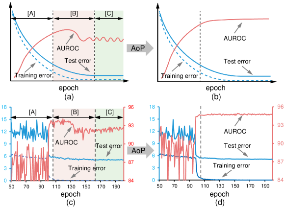
Figure 1: (a) shows the concepts of overfitting and instability, which harms OOD detection. [A] shows the test error decreases and AUROC increases. [B] also shows test error decreases, while AUROC decreases dramatically. [C] shows the test accuracy is stable while AUROC shows instability. We avoid these two drawbacks by AoP, visualized in (b). These claims are confirmed by experiments shown in (c)-(d). The model is a ResNet-18 [15] trained on CIFAR-10 [25], and OOD dataset is LSUN [51].

One core issue of detecting OOD samples is to design a detector $\phi\left(\boldsymbol{x}\right)$ that maps an input $\boldsymbol{x}$ to a scalar to distinguish OOD data from in-distribution (ID). In the test stage, given a threshold $\delta$, samples are regarded as OOD data if $\phi\left(\boldsymbol{x}\right)>\delta$, and as ID otherwise. By changing the threshold, AUROC, i.e., the area under Receiver Operating Characteristics (ROC) curve is calculated, which is a threshold-independent metric in OOD detection.

Recently, there has been great progress in detecting OOD data. Various scoring functions are designed to distinctly distinguish the output scores of ID and OOD data, like ODIN [31], Mahalanobis distance [29], energy score [33] and ViM [47]. Besides, one of the most effective methods up to now, called Outlier Exposure (OE) [17], is to train the models against auxiliary data of natural outlier images. With the rapid advances in model architecture like vision transformer [5], it has also been empirically verified that transformer outperforms convolutional neural network in OOD detection [9].

Despite the success of previous methods, less attention has been given to the chaotic behavior of OOD detection along the optimization trajectory during training. For example, it remains elusive how the curve of AUROC changes during training. In this paper, we first delve into analyzing the curve of metrics in OOD detection in training stage. As shown in Figure 1(a), our findings reveal that the curve of AUROC could be decomposed into three stages: In the first stage, i.e. stage [A], both the training error and test error are decreasing, and AUROC is increasing. In the second stage, i.e. stage [B], test error continues decreasing when the training error approaches near zero, while AUROC is decreasing like overfitting. This phenomenon of overfitting greatly harms OOD detection. In the third stage, i.e. stage [C], AUROC varies greatly during training, while the test error is much more stable. The instability of AUROC makes the choice of final model not reliable, because a nearby checkpoint may achieve a much better or worse performance in OOD detection. The overfitting and instability of AUROC during training greatly harm the performance of OOD detection, which is neglected by previous methods.

In this paper, we first analyze the problem of instability. The instability mainly comes from the vulnerability of model to the small perturbations of weight [2] during training. We show that a small perturbation of the final checkpoint could cause AUROC to vary sharply. To alleviate the instability of OOD detection during training, we utilize the moving averaged model as our final model, whose parameters are determined by the moving average of the online model’s parameters. Model averaging could lead to a flat loss landscape [23], which makes AUROC more stable during training. With the help of model averaging, it is more reliable to choose the final checkpoint as the model deployed in practical scenarios.

Next, we investigate why the overfitting happens, and then propose its solution. For an over-parameterized model, continuing training model after reaching near zero training error would drive the model to memorize training data [53]. The memorization drives model to learn redundant and noisy features which commonly exist in different datasets, thus causing the overlap of distribution between ID and OOD data. Consequently, the model becomes overfitting in OOD detection. To alleviate the overfitting, our key idea is to employ a global sparsity constraint as a method to evade memorizing training data and learning noisy features, which is closely related to network pruning [13]. We theoretically show that LASSO [46] largely eliminates the problem of overfitting based on a linear model, which motivates us to use pruning in neural networks.

Combining the two issues above, we summarize our method as Average of Pruning (AoP), and AoP could be regarded as a simple module readily pluggable into any existing method in OOD detection. It is empirically verified that AoP achieves significant improvement on OOD detection. Our contributions can be summarized as follows:

• We uncover the phenomenon of instability and overfitting in OOD detection during training, which seriously affects performance.

• We verify that instability comes from the vulnerability of model to small changes in weights, and overfitting is reduced by overparameterization which drives model to learn noisy and abundant features.

• We propose Average of Pruning. Model averaging improves stability and pruning eliminates overfitting.

• We conduct comprehensive experiments and ablation studies to verify the effectiveness of AoP, across different datasets and network architectures.

2 Related Work

OOD Detection Various methods are proposed under the setting that whether use the auxiliary data of natural outliers or not. The work of [16] first introduced a baseline called MSP as the scoring function to detect OOD inputs. Later, various methods focus on designing scoring functions are proposed [31, 28, 33, 42, 47, 43]. Generative models [39] are also applied to provide reliable estimations of confidence. Besides, OE [17] first introduced an extra dataset consisting of outliers in training and enforced low confidence on such outliers. To better utilize the auxiliary dataset, different methods are propose [50, 34]. There are also some methods to synthesize outliers [6].

Model Averaging The basic idea of model averaging could refer to tail-averaging [24], which averages the final checkpoints of SGD, and it could decrease the variance induced by SGD noise and stabilize training [37]. Further, stochastic weight averaging [23] applies cyclical learning rate to average the selected checkpoints. It has been empirically verified that model averaging contributes to a flatter loss landscape and wider minimum [23]. Based on this, we investigate whether OOD detection suffers from instability in training, which is an essential issue neglected before.

Pruning and sparsity We mainly discuss unstructured pruning. The concept of pruning in neural networks dated back to [27]. To reduce the memory in modern neural networks, pruning has attracted great attention [13] recently. Methods are proposed to drop the unimportant weights [13, 55, 7, 32]. The goal of pruning is to deploy modern networks with a slight loss of generalization. Among these, the lottery ticket hypothesis (LTH) [10, 11] shows that sparse networks training from scratch can reach full accuracy than dense networks. Previous works focus on the generalization of pruned models, while we discuss the connection between sparsity and OOD detection.

3 Model Averaging Improves Stability

In this section, we first instability analysis of the final checkpoint on OOD detection. Then, we show that model averaging could largely make the performance more stable.

3.1 Motivation: Instability Analysis

Previous methods like scoring functions focus on post-hoc process, while the instability of final checkpoint on OOD detection is neglected. To be more specific, a nearby checkpoint may achieve much better or worse performance. As shown in Fig. 1(c), AUROC varies sharply in the final stage, which makes the performance of final checkpoint unreliable. We also find that post-hoc process could not alleviate such instability, as shown in Fig 2(a).

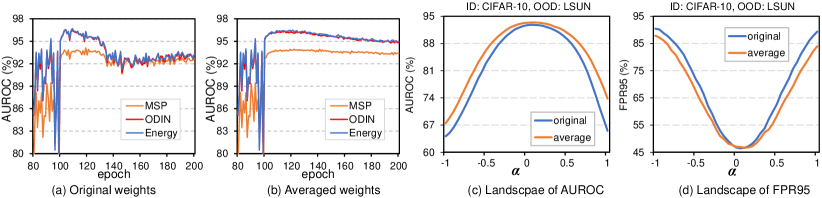
Figure 2: (a)-(b): Influence of different scoring functions. Different scoring function [31, 33] also suffer from instability. (c)-(d): Landscape of AUROC ($\uparrow$) and FPR95 ($\downarrow$) under weight perturbations for the original model and averaged model.

Visualization. To better investigate how the changes in weights influence the performance of OOD detection, we visualize AUROC and FPR95 landscape by plotting their value changes when moving the weights along a random direction $d$ with magnitude $\alpha$:

$$\theta\left(d,t\right)=\theta_{\mathrm{final}}+\alpha\cdot d,$$

where $d$ is a random direction drawn from a Gaussian distribution and repeated 10 times. The random direction is normalized as proposed in [30]. The visualization of a trained ResNet-18 [15] is shown in Fig. 2(c).

Based on the landscape of AUROC and FPR95, we find that the solution is fragile under small perturbations of weights, resulting narrow optima in OOD detection. Intuitively, wider optima would make the performance of OOD detection more stable, since the changes of weights may have less influence on performance.

3.2 Method: Model Averaging

To contribute to a wider optimum, we adopt Stochastic Weight Averaging (SWA) [23], which aims to find much broader optima for better generalization. SWA averages multiple points along the trajectory of SGD with a cyclical or constant learning rate. In this paper, we implement SWA using a simply exponential moving average $\theta_{t}^{\mathrm{MA}}$ of the original model parameters $\theta_{t}$ with a decay rate $\tau$ after epoch $t_{0}$, called as Model Averaging (MA):

$$\theta_{t+1}^{\mathrm{MA}}=\left\{\begin{array}[]{c}\theta_{t},\,\,\,\,t<t_{0}\\ \tau\cdot\theta_{t}^{\mathrm{MA}}+\left(1-\tau\right)\cdot\theta_{t+1},\,\,\,\,t\geq t_{0}\\ \end{array}\right.,$$ (1)

where $\tau=\frac{t-t_{0}}{t-t_{0}+1}$ is a constant. In the stage of evaluation, the weighted parameters $\theta_{t}^{\mathrm{MA}}$ are used instead of the originally trained models $\theta_{t}$. As shown in Fig. 2(b), the averaged model achieves a more stable performance. MA is also shown to stabilize the performance of various scoring functions, as shown in Fig. 2(d). The performance on OOD detection is expected to be smoother since the weights of MA are the average of nearby checkpoints.

MA could be interpreted as approximating FGE ensemble [12] with a single model. Ensembling has been verified to boost the performance of OOD detection before [26]. However, such ensemble methods require the practicer to train multiple classifiers, which induces much extra computational budget, while MA is more convenient and has almost no computational overhead.

4 Pruning Eliminates Overfitting

In this section, we first reveal that an over-parameterized model may cause overfitting in OOD detection during training, and then show that increasing the sparsity of model by pruning could eliminate it based on theoretical analysis.

4.1 Motivation: Overfitting Analysis

The training trajectory of models in OOD detection has not been explored clearly before. As shown in Fig. 1 (a)(c), OOD detection suffers from overfitting, and so does the averaged model in Fig. 2(b). We would like to provide more evidence on such overfitting.

More empirical verifications. We conduct experiments on WideResNet-28 [52] with various width factors, and the results are shown in Fig 3. We can see as the width increases, the test accuracy increases steadily while AUROC first increases and then decreases. This verifies that OOD detection is harmed by overfitting from overparameterization.

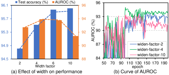
Figure 3: Influence of different width in WideResNet [52]. (a) As width increases, test accuracy increases while AUROC first increases and then decreases. (b) Curves of AUROC during training.

Theoretical Analysis. Suppose we have an ID dataset $\mathcal{D}_{\mathrm{ID}}$ consist of samples $(\boldsymbol{x},y)$ and an OOD dataset $\mathcal{D}_{\mathrm{OOD}}$ with samples $(\boldsymbol{x},q)$. Formally, we set the $d+1$ dimension features $\boldsymbol{x}=\left(x_{1},x_{2},\cdots,x_{d+1}\right)$ of ID and OOD data are drawn according to Gaussian distributions:

$$\begin{aligned} y&\overset{u.a.r}{\sim}\left\{-1,+1\right\},\,\,\,\boldsymbol{x}\sim\mathcal{N}\left(y\cdot\boldsymbol{\mu}_{\mathrm{ID}},\sigma^{2}\boldsymbol{I}\right)\\ q&\overset{u.a.r}{\sim}\left\{-1,+1\right\},\,\,\,\boldsymbol{x}\sim\mathcal{N}\left(q\cdot\boldsymbol{\mu}_{\mathrm{OOD}},\sigma^{2}\boldsymbol{I}\right)\end{aligned},$$ (2)

where $\boldsymbol{\mu}_{\mathrm{ID}}=\left(1,\eta,\cdots,\eta\right)$ and $\boldsymbol{\mu}_{\mathrm{OOD}}=\left(0,\eta,\cdots,\eta\right)\in\mathbb{R}^{d+1}$. The distribution of $(x_{1})$ is different for ID and OOD data, which is called as special feature because it reveals the difference between ID and OOD data. The distribution of the rest features $\left(x_{2},\dots,x_{d+1}\right)$ are the same for ID and OOD data, which are called as common features because they may induce overlap for ID and OOD data. Usually, the common features mean various noise rather than semantic information, so they are often less discriminative but abundant [22, 44, 45], i.e., $0<\eta\ll 1$ and $d\gg 1$.

The Bayes optimal classifier $f_{\mathrm{Bayes}}\left(\boldsymbol{x}\right)$ could be derived based on the distribution of ID data. Then, the decision is based on the sign of logits from Bayes classifier, i.e.,

$$f_{\mathrm{Bayes}}\left(\boldsymbol{x}\right)=x_{1}+\eta\sum_{i=2}^{d+1}{x_{i}}.$$ (3)

Definition 4.1 (ID classification risk, OOD detection risk).

For a classifier $f$, the risks induced by classification on ID data $\mathcal{R}_{\mathrm{ID}}\left(f\right)$ and rejection on OOD data $\mathcal{R}_{\mathrm{OOD}}\left(f\right)$ are

$$\mathcal{R}_{\mathrm{ID}}\left(f\right)=\underset{\left(\boldsymbol{x},y\right)\sim\mathcal{D}_{\mathrm{ID}}}{\mathrm{Pr}}\left\{\mathrm{sign}(f\left(\boldsymbol{x}\right))\neq y\right\},$$ (4)

$$\mathcal{R}_{\mathrm{OOD}}\left(f\right)=\underset{\left(\boldsymbol{x},q\right)\sim\mathcal{D}_{\mathrm{OOD}}}{\mathrm{Pr}}\left\{\left|f\left(\boldsymbol{x}\right)\right|>\delta\right\},$$

where $\delta$ is a given threshold for detecting OOD data. Inputs are accepted as ID data when the magnitude of their logits are larger than the threshold.

Theorem 4.2.

Suppose the distributions of ID and OOD data follow Gaussian distribution in Eq. (2), then $\mathcal{R}_{\mathrm{ID}}\left(f_{\mathrm{Bayes}}\right)$ and $\mathcal{R}_{\mathrm{OOD}}\left(f_{\mathrm{Bayes}}\right)$ could be simplified to

$$\mathcal{R}_{\mathrm{ID}}\left(f_{\mathrm{Bayes}}\right)=\,\,\mathrm{Pr}\left\{\mathcal{N}\left(0,1\right)>\frac{\sqrt{1+d\eta^{2}}}{\sigma}\right\},$$ (5)

$$\mathcal{R}_{\mathrm{OOD}}\left(f_{\mathrm{Bayes}}\right)=\mathrm{Pr}\left\{\mathcal{N}\left(0,1\right)>\frac{\delta-d\eta^{2}}{\sigma\cdot\sqrt{1+d\eta^{2}}}\right\}+\mathrm{Pr}\left\{\mathcal{N}\left(0,1\right)>\frac{\delta+d\eta^{2}}{\sigma\cdot\sqrt{1+d\eta^{2}}}\right\}.$$

Theorem C.1 indicates that the number of common features $d$ has a close connection with accuracy and OOD detection performance. For clearer understanding, a detailed example is shown in Fig 4(a) with concrete settings. As $d$ increases, $\mathcal{R}_{\mathrm{ID}}\left(f_{\mathrm{Bayes}}\right)$ decreases slowly while $\mathcal{R}_{\mathrm{OOD}}\left(f_{\mathrm{Bayes}}\right)$ increases sharply. We could conclude that an approximately small value of $d$ contributes a better trade-off between classification and OOD detection. The curves of OOD detection risk with different rejection thresholds $\delta$ are also given, and they show a consistent tendency.

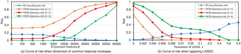
Figure 4: A detailed example on how the number of common features $d$ and LASSO influence $\mathcal{R}_{\mathrm{ID}}\left(f\right)$ (i.e., ID classification risk) and $\mathcal{R}_{\mathrm{OOD}}\left(f\right)$ (i.e., OOD detection risk). As a concrete example, here we set $\sigma=1,\eta=0.01$. In (b), we keep $d=50000$.

If the model is over-parameterized, it is reasonable to use feature selection to reduce the over-much common features to improve performance on OOD detection. We would show that the well-known method in feature selection LASSO [46] could achieve this goal. The solution with LASSO could be obtain by optimizing the overall loss [14]:

$$\underset{\boldsymbol{w}}{\min}\,\,\mathbb{E}_{\left(\boldsymbol{x},y\right)\sim\mathcal{D}_{\mathrm{ID}}}\left\{\frac{1}{2}\left(\boldsymbol{w}^{T}\frac{\boldsymbol{x}}{\sigma}-y\right)^{2}+\lambda\cdot\left|\boldsymbol{w}\right|_{1}\right\},$$ (6)

where $\lambda$ is the parameter of LASSO.

Theorem 4.3.

The classifier $f_{\mathrm{LASSO}}$ [14] obtained by minimizing the loss in Eq. (6) is

$$f_{\mathrm{LASSO}}\left(\boldsymbol{x}\right)=\left(\left(1-\lambda\right)_{+}\cdot x_{1}+\sum_{i=2}^{d+1}{\left(\eta-\lambda\right)_{+}\cdot x_{i}}\right),$$ (7)

where $\left(\cdot\right)_{+}$ means the positive part of a number.

For intuitive understanding of Theorem C.2, we draw $\mathcal{R}_{\mathrm{ID}}$ and $\mathcal{R}_{\mathrm{OOD}}$ for $f_{\mathrm{LASSO}}$ while changing the parameter $\lambda$ in LASSO, and the results are shown in Fig. 4(b). As $\lambda$ increases, $\mathcal{R}_{\mathrm{OOD}}$ rapidly decreases and $\mathcal{R}_{\mathrm{ID}}$ increases. A better trade-off could be achieved while $\lambda\approx\eta=0.01$.

4.2 Method: Lottery Tickets Hypothesis

As shown in the previous analysis, overparameterization causes the models to learn more noisy and redundant features, which results in overfitting in OOD detection. We also show LASSO [46] is a promising method. However, LASSO is not suitable for neural networks. For deep models, pruning aims to construct sparse models.

For a neural network $f\left(x;\theta\right)$ with parameters $\theta$, its pruned model could be denoted as $f\left(x;m\odot\theta\right)$ with a set of binary masks $m\in\left\{0,1\right\}^{n}$, where $\odot$ means the element-wise product and $n$ is the number of parameters. One effective method is the Lottery Ticket Hypothesis (LTH) [10], which adopts iterative magnitude pruning (IMP).

In this paper, we adopt the commonly used LTH with weight rewinding [11] to find the sparse subnetworks. Pseudo-code is provided in Algorithm 1, and it seems similar to the solution of LASSO for the linear model in Eq. (C.2).

In the original paper of LTH [10], it is claimed that dense randomly-initialized neural networks contain a sparse subnetwork that can be trained in isolation to match the test accuracy of the original network. However, this hypothesis has not been introduced to OOD detection. In this paper, we propose that pruning [13] (e.g, LTH) also helps OOD detection by alleviating overfitting. As shown in Fig 5, when we increase the sparsity of model, the overfitting in OOD detection during training becomes weaker, and thus we achieve a better performance in the final checkpoint.

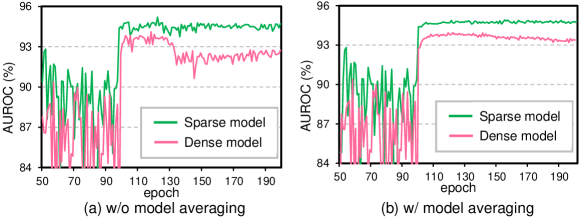
Figure 5: Effect of pruning on eliminating overfitting. The settings are the same as Fig. 1.

In practical applications, large networks are often compressed to reduce the number of weights or the memory footprint [13] because of the memory limits. Our results show that one of the byproducts of a pruned model is the improvement in detecting unknown inputs, which is essential in practical scenarios. We will also provide comparisons with other pruning methods in the latter section.

Algorithm 1 IMP weight rewinding for LTH

0:  Rewinding step $k$, training steps $T$, pruning iterations $N$.

0:  Learned weights $\theta$, pruning mask $m$.

  Randomly initialize network $f$ with initial weights $\theta_{0}\in\mathbb{R}^{d}$.

  Initialize pruning mask to $m=1^{d}$.

  Train $\theta_{0}$ to $\theta_{k}$ for $k$ steps.

  for $n=1,\cdots,N$ do

     Train $m\odot\theta_{k}$ to $m\odot\theta_{T}$.

     Prune the 20% lowest-magnitude weights globally and get mask $m$.

     Rewind the weights to $\theta_{k}$.

  end for

4.3 Overall Method: Average of Pruning

Combining model averaging and pruning, we propose Average of Pruning (dubbed AoP) to boost OOD detection performance. As many of the effective OOD detection methods are post-hoc processes, AoP could be easily applied as a simple module readily pluggable into any existing method. The pipeline is divided as follows:

5 Experiments

In this section, we evaluate AoP on various OOD detection tasks. We first verify the effectiveness of AoP on CIFAR benchmarks and provide comprehensive ablation studies. Then, we proceed with ImageNet benchmark.

5.1 Evaluation on CIFAR Benchmarks

In-distribution Datasets. We use CIFAR-10 and CIFAR-100 [25] as in-distribution data.

Table 1: Performance of OOD detection for various methods on CIFAR benchmarks. All the metrics on OOD detection are the average on six OOD datasets. All values are percentages. The best results are boldfaced for highlight.

Model	Methods	Reference	In-distribution dataset: CIFAR-10				In-distribution dataset: CIFAR-100
			AUROC $\uparrow$	AUPR $\uparrow$	FPR95 $\downarrow$	Acc $\uparrow$	AUROC $\uparrow$	AUPR $\uparrow$	FPR95 $\downarrow$	Acc $\uparrow$
ResNet-18	MSP [16]	ICLR2017	91.63 $\pm$ 0.26	98.08 $\pm$ 0.11	50.00 $\pm$ 0.50	94.98 $\pm$ 0.11	76.64 $\pm$ 0.20	94.31 $\pm$ 0.08	80.03 $\pm$ 0.72	75.83 $\pm$ 0.33
	ODIN [31]	ICLR2018	92.13 $\pm$ 0.96	97.92 $\pm$ 0.36	36.19 $\pm$ 3.47	94.98 $\pm$ 0.11	81.05 $\pm$ 0.83	95.44 $\pm$ 0.18	74.04 $\pm$ 2.53	75.83 $\pm$ 0.33
	Maha [29]	NeurIPS2018	90.61 $\pm$ 1.13	97.88 $\pm$ 0.24	45.31 $\pm$ 4.63	94.98 $\pm$ 0.11	74.36 $\pm$ 0.64	92.88 $\pm$ 0.13	71.97$\pm$ 2.15	75.83 $\pm$ 0.33
	Energy [33]	NeurIPS2020	92.24 $\pm$ 1.02	97.96 $\pm$ 0.35	35.15 $\pm$ 3.43	94.98 $\pm$ 0.11	81.36 $\pm$ 0.87	95.50 $\pm$ 0.18	72.29 $\pm$ 2.78	75.83 $\pm$ 0.33
	GradNorm [21]	NeurIPS2021	50.04 $\pm$ 5.55	81.79 $\pm$ 2.59	84.18 $\pm$ 2.53	94.98 $\pm$ 0.11	69.78 $\pm$ 3.63	90.69 $\pm$ 1.81	74.91 $\pm$ 1.08	75.83 $\pm$ 0.33
	ReAct [42]	NeurIPS2021	92.46 $\pm$ 0.73	98.19 $\pm$ 0.52	34.63 $\pm$ 2.80	94.98 $\pm$ 0.11	80.35 $\pm$ 0.52	95.36 $\pm$ 0.11	76.20 $\pm$ 2.01	75.83 $\pm$ 0.33
	MaxLogit [18]	ICML2022	92.61 $\pm$ 0.29	98.13 $\pm$ 0.07	35.09 $\pm$ 1.90	94.98 $\pm$ 0.11	81.02 $\pm$ 0.84	95.44 $\pm$ 0.17	74.13 $\pm$ 2.64	75.83 $\pm$ 0.33
	VOS [48]	ICLR2022	93.54 $\pm$ 1.05	98.47 $\pm$ 0.28	32.90 $\pm$ 5.02	94.67 $\pm$ 0.14	81.14 $\pm$ 1.02	95.40 $\pm$ 0.36	74.46 $\pm$ 3.54	74.66 $\pm$ 0.26
	KNN [43]	ICML2022	94.39 $\pm$ 0.27	98.65 $\pm$ 0.24	34.42 $\pm$ 0.58	94.98 $\pm$ 0.11	80.43 $\pm$ 0.88	94.84 $\pm$ 0.32	69.72 $\pm$ 1.84	75.83 $\pm$ 0.33
	+ AoP	-	95.04 $\pm$ 0.17	98.88 $\pm$ 0.04	25.30 $\pm$ 1.63 $\downarrow$ 9.1	94.89 $\pm$ 0.11	84.36 $\pm$ 0.71	96.12 $\pm$ 0.22	58.01 $\pm$ 1.08 $\downarrow$ 11.7	76.08 $\pm$ 0.15
	ViM [47]	CVPR2022	94.18 $\pm$ 0.26	98.68 $\pm$ 0.04	32.27 $\pm$ 1.02	94.98 $\pm$ 0.11	81.03 $\pm$ 1.84	95.53 $\pm$ 0.45	72.90 $\pm$ 5.91	75.83 $\pm$ 0.33
	+ AoP	-	95.69 $\pm$ 0.19	99.08 $\pm$ 0.04	25.3 $\pm$ 1.63 $\downarrow$ 7.0	94.89 $\pm$ 0.11	86.16 $\pm$ 0.71	96.76 $\pm$ 0.18	59.28 $\pm$ 2.77 $\downarrow$ 13.6	76.08 $\pm$ 0.15
WRN-28-10	MSP [16]	ICLR2017	91.24 $\pm$ 0.08	97.72 $\pm$ 0.05	46.21 $\pm$ 1.72	95.70 $\pm$ 0.07	75.77 $\pm$ 0.58	93.92 $\pm$ 0.26	81.53 $\pm$ 0.40	79.72 $\pm$ 0.22
	ODIN [31]	ICLR2018	92.35 $\pm$ 0.31	97.78 $\pm$ 0.13	30.63 $\pm$ 0.86	95.70 $\pm$ 0.07	81.25 $\pm$ 0.68	95.42 $\pm$ 0.19	74.28 $\pm$ 1.64	79.72 $\pm$ 0.22
	Maha [29]	NeurIPS2018	94.30 $\pm$ 0.37	98.75 $\pm$ 0.08	28.82 $\pm$ 1.94	95.70 $\pm$ 0.07	63.32 $\pm$ 1.46	88.83 $\pm$ 0.57	79.36 $\pm$ 1.08	79.72 $\pm$ 0.22
	Energy [33]	NeurIPS2020	92.49 $\pm$ 0.32	97.82 $\pm$ 0.14	29.72 $\pm$ 0.99	95.70 $\pm$ 0.07	78.03 $\pm$ 0.43	94.47 $\pm$ 0.11	78.65 $\pm$ 1.40	79.72 $\pm$ 0.22
	GradNorm [21]	NeurIPS2021	47.70 $\pm$ 2.68	85.35 $\pm$ 5.52	87.45 $\pm$ 2.02	95.70 $\pm$ 0.07	64.90 $\pm$ 2.60	89.18 $\pm$ 1.07	81.82 $\pm$ 2.40	79.72 $\pm$ 0.22
	ReAct [42]	NeurIPS2021	82.80 $\pm$ 1.60	95.93 $\pm$ 0.33	69.93 $\pm$ 6.42	95.70 $\pm$ 0.07	84.09 $\pm$ 1.58	96.33 $\pm$ 0.38	68.46 $\pm$ 5.91	79.72 $\pm$ 0.22
	MaxLogit [18]	ICML2022	92.35 $\pm$ 0.27	97.78 $\pm$ 0.13	30.48 $\pm$ 0.87	95.70 $\pm$ 0.07	77.82 $\pm$ 0.56	94.41 $\pm$ 0.16	79.40 $\pm$ 1.18	79.72 $\pm$ 0.22
	VOS [6]	ICLR2022	91.01 $\pm$ 1.49	95.46 $\pm$ 2.42	30.98 $\pm$ 4.65	95.70 $\pm$ 0.07	80.84 $\pm$ 1.34	95.24 $\pm$ 0.40	73.66 $\pm$ 3.31	79.79 $\pm$ 0.20
	KNN [43]	ICML2022	94.40 $\pm$ 0.14	98.79 $\pm$ 0.04	32.74 $\pm$ 0.82	95.70 $\pm$ 0.07	80.50 $\pm$ 0.56	95.03 $\pm$ 0.26	69.68 $\pm$ 0.91	79.72 $\pm$ 0.22
	+ AoP	-	95.89 $\pm$ 0.03	99.12 $\pm$ 0.02	23.95 $\pm$ 0.08 $\downarrow$ 8.8	96.00 $\pm$ 0.15	83.61 $\pm$ 0.30	95.88 $\pm$ 0.11	63.04 $\pm$ 1.06 $\downarrow$ 6.6	80.36 $\pm$ 0.18
	ViM [47]	CVPR2022	96.31 $\pm$ 0.28	99.12 $\pm$ 0.08	18.35 $\pm$ 1.46	95.70 $\pm$ 0.07	84.04 $\pm$ 0.95	96.13 $\pm$ 0.28	62.41 $\pm$ 1.58	79.72 $\pm$ 0.22
	+ AoP	-	96.53 $\pm$ 0.20	99.14 $\pm$ 0.06	15.83 $\pm$ 0.24 $\downarrow$ 2.7	96.00 $\pm$ 0.15	85.72 $\pm$ 0.45	96.60 $\pm$ 0.16	58.71 $\pm$ 1.03 $\downarrow$ 3.7	80.36 $\pm$ 0.18

Out-of-distribution Datasets. For the OOD datasets, we use six common benchmarks as used in previous study [33, 42, 40]: Textures [3], SVHN [36], LSUN-Crop [51], LSUN-Resize [51], Place365 [54], and iSUN [49]. The detailed information of datasets is presented in the appendix. We would like to clarify that the CIFAR benchmark are different from those in the earlier work [16, 29, 31]. These new OOD datasets are harder than the earlier OOD dataset like Uniform noise. As shown by recent work [33, 40], most existing baselines are far not up to perfect OOD detection performance on this new CIFAR benchmark.

Evaluation Metrics. We use the common metrics to measure the quality of OOD detection: (1) the area under the receiver operating characteristic curve (AUROC); (2) the area under the precision-recall curve (AUPR); (3) the false positive rate of OOD samples when the true positive rate of in-distribution samples is at 95% (FPR95).

Training Details. ResNet-18 [15] and WideResNet-28-10 [52] are the main backbones for all methods, and the model is trained by momentum optimizer with the initial learning rate of 0.1. We set the momentum to be 0.9 and the weight decay coefficient to be $2\times 10^{-4}$. Models are trained for 200 epochs and the learning rate decays with a factor of 0.1 at 100 and 150 epochs. Other hyper-parameters for the OOD detection methods come from reference code [50] and the original work. We apply LTH with learning weight rewind [11]. We prune 20% of the weights in each pruning stage and repeat 9 times (reaching around a sparsity of 90%). We run each trial 5 times.

AoP boosts OOD detection. A detailed experiments for comparison with mostly recent methods are conducted, and the results are listed in Tab. 1. AoP could apply to the existing method KNN [43] and ViM [47], and boost their performance significantly. The performance of pruned model based on MSP [16] when we iteratively prune the network is shown in Figure 6. The models with remaining weights of 100% mean the dense model without pruning. The performance of pruned models outperforms dense models in a wide range of sparsity. As the sparsity of model increases, the performance of model on OOD detection first rises and then falls. This variation tendency is consistent with intuition since overly pruning the model will make the model lose some important weights.

AoP boosts various OOD scoring functions. Since AoP is a simple module readily pluggable into the existing methods, we add it to other methods. We report the results of adding AoP to MSP [16] and MaxLogit [18], and it shows consistent improvement in Fig. 7 and Tab. 2.

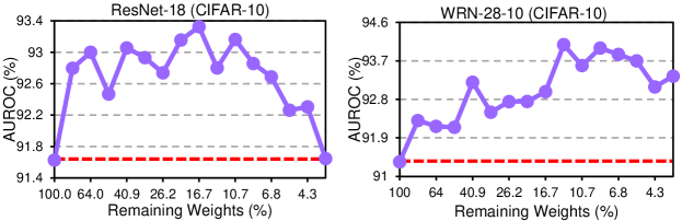
Figure 6: Performance on OOD detection (AUROC) based on MSP [16] under different sparsity in AoP. The backbone and training dataset are listed in the title of figure. We draw the red horizontal line with a value of performance in the dense model.

Figure 7: Distribution of MSP [16]scores v.s. MSP+AoP scores. The model distinguishes OOD data better while using AoP.

Table 2: Performance on OOD detection under other scoring functions. The model is ResNet-18 [15] trained on CIFAR-10 [25].

Method	MSP			MaxLogit
	AUROC	AUPR	FPR95	AUROC	AUPR	FPR95
w/ o AoP	91.63	98.08	50.00	92.61	98.13	35.09
w / AoP	93.32 $\uparrow$ 1.7	98.64	45.95 $\downarrow$ 4.0	95.53 $\uparrow$ 2.9	99.06	25.80 $\downarrow$ 9.3

Table 3: Performance on OOD detection with OE [17]. The model is ResNet-18 [15] trained on CIFAR-10 [25].

Method	AUROC	AUPR	FPR95	Acc
OE	98.66	99.73	4.49	93.92
+ AoP	98.91	99.78	3.85	94.00

AoP is compatible with OE. OE [17] leverages a dataset of known outliers during training, which is a very strong baseline in OOD detection. A recent study [1] finds that many methods using auxiliary datasets are equivalent to OE, so we just use OE as the baseline on the behalf of these methods that use extra data. The outlier exposure dataset used in this experiment is 300K Random Images [17]. The performance is listed in Tab. 3. The results show that AoP can achieve consistent improvement on OE.

AoP is beneficial for near-OOD detection tasks. The difficulty of detecting OOD inputs relies on how semantically close the unknowns are to the inlier classes, which contributes to near-OOD task and far-OOD task. For example, for a model trained on CIFAR-10, it is hard to detect inputs from CIFAR-100 than SVHN, and the former is regarded as a near-OOD task. A recent study [40] reveals that none of the methods are good at detecting both near and far OOD samples except OE [17]. As shown in Fig. 8, AoP is helpful in near-OOD task.

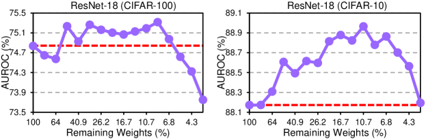
Figure 8: Performance of near OOD detection. In-distribution data is CIFAR-100 and OOD data is CIFAR-10, and vice versa. Backbone used is ResNet-18 [15].

5.2 Evaluation on ImageNet Benchmarks

In-distribution Datasets. We use Tiny-ImageNet and ImageNet [4] as the in-distribution dataset. Tiny-ImageNet is a 200-class subset of ImageNet where images are resized and cropped to 64$\times$64 resolution. The training set has 100,000 images and the test set has 10,000 images.

Out-of-distribution Datasets. For the OOD datasets, we use the common benchmarks used in [33]: Textures [3], iSUN [49], LSUN-Resize [51], and Place365 [54].

Training Details. For Tiny-ImageNet, the settings are the same as CIFAR benchmarks. For ImageNet, we use one-shot pruning to achieve the sparsity of 80%, and other settings are the same as [32].

Results. The results for Tiny-ImageNet are listed in Tab. 4. It reveals that the model with AoP achieves great improvement in OOD detection on three datasets. We also provide the results on ImageNet in Tab. 5. These three OOD datasets follow MOS [20]. The results show AoP achieves consistent improvement.

Table 4: OOD detection performance on Tiny-ImageNet using ResNet-18 [15]. The best results are boldfaced for highlight.

Method	Textures			LSUN			iSUN
	AUROC	AUPR	FPR95	AUROC	AUPR	FPR95	AUROC	AUPR	FPR95
MSP [16]	68.32	91.87	89.17	63.79	90.89	93.8	64.76	91.14	92.71
+ AoP	71.61	93.08	86.35	66.85	91.82	91.77	66.29	91.47	91.20
ODIN [16]	69.03	90.08	87.45	57.87	88.70	94.22	61.22	89.49	91.46
+ AoP	74.02	93.12	81.98	61.65	90.07	93.18	63.55	90.17	90.10
Energy [16]	69.01	90.81	86.09	57.25	88.51	93.75	60.85	89.36	91.25
+ AoP	74.13	93.12	80.16	60.94	89.88	92.45	63.23	90.07	89.38

Table 5: Performance of OOD detection on ImageNet [4] using ResNet-50 [15].

Dataset	MSP	+ AoP	ODIN	+ AoP	Energy	+ AoP	MaxLogit	+ AoP	ViM	+ AoP
Places	76.26	76.58	72.91	73.90	68.41	68.49	73.73	76.40	84.74	84.91
SUN	77.58	78.24	74.10	75.52	69.68	70.32	74.75	76.91	86.87	87.59
Textures	78.58	78.91	75.88	76.86	73.90	74.97	77.80	79.32	98.27	98.73

5.3 Ablation Studies

Effectiveness of MA and pruning. To verify the importance of the two components in AoP, we test the performance of OOD detection when they are not used. The results are listed in Tab. 6. As shown in the table, both of them are essential in OOD detection.

Table 6: Effectiveness of MA and pruning. The in-distribution dataset is CIFAR-10.

MA	pruning	ResNet-18			WideResNet-28-10
		AUROC	AUPR	FPR	AUROC	AUPR	FPR
✗	✗	91.63	98.08	50.00	91.24	97.72	46.21
✗	✔	92.94	98.51	46.19	93.43	98.22	41.55
✔	✔	93.32	98.64	45.95	93.99	98.66	37.22

Table 7: Effectiveness of the three during training pruning techniques. The model is a ResNet-18 [15] trained on CIFAR-10.

Methods	Sparsity: 60%		Sparsity: 80%		Sparsity: 90%
	AUROC	Acc	AUROC	Acc	AUROC	Acc
GMP [55]	92.13	94.88	92.54	94.33	92.53	94.32
RigL [7]	92.66	94.25	92.37	93.95	92.51	94.08
GraNet [32]	93.14	94.59	92.75	94.54	92.99	94.41

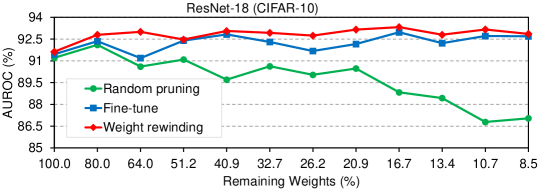
Figure 9: Influence of different iterative pruning strategies. The model is a ResNet-18 [15] trained on CIFAR-10.

Influence of pruning techniques. (1) Different iterative pruning methods. LTH is a kind of iterative pruning [10, 11]. We compare it with other two iterative pruning strategies: random pruning and fine-tuning [10]. The results on CIFAR-10 are shown in Fig. 9. It shows that LTH with weight rewind achieves the best performance. The performance of fine-tuning is poorer, verifying that the initialization of weights is important in OOD detection. Random pruning decreases the performance, revealing that the weights can not be dropped arbitrarily. (2) During-training pruning methods.

Figure 10: The difference of extracted feature between ID and OOD data. Features extracted by dense model seem to be similar, while it is distinct for sparse model.

Since LTH is a kind of post-training pruning, we also explore whether during-training pruning is beneficial for OOD detection. We show the performance of three methods: GMP [55], RigL [7], and GraNet [32]. The settings about pruning mainly follow GraNet [32]. The results are listed in Tab. 7. These pruning techniques are good for OOD detection, while they are poorer than LTH [11].

Effectiveness on other networks. We conduct more experiments on other networks to verify that AoP promotes OOD detection, including Vgg-16 [41], WideResNet-40-2 [52] and MobileNet [19]. AoP achieves consistent promotion. To save space, results are shown in the appendix.

Visualization of features. To show the influence of AoP on feature representation in OOD detection, we visualize the final features. We randomly sample a batch of data from CIFAR-10 [25] (ID data) and LSUN [51] (OOD data), and calculate the difference of feature representations for dense models. We also calculate the difference for sparse model. We visualize the absolute value of difference of final features. The results are shown in Fig. 10. In the figure, most of the features from ID or OOD dataset are similar for dense model. However, their difference are more obvious for sparse model. It verifies that the sparsity drives model to drop common features existing in both ID and OOD datasets.

5.4 AoP Improves Misclassification Detection

Background. We investigate the effect of AoP on Misclassification Detection (MD). OOD detection and MD both reflect whether models know what they do not know. In safety-critical settings, the classifier should output lower confidence for both incorrect predictions from known classes and OOD examples from unknown (new) classes. The benchmarks of these two tasks are proposed and studied together in [16, 35]. We study these two tasks to provide a more comprehensive evaluation, which can better verify the effect of our findings.

Setups. The hyper-parameters for models are the same as settings in Sec. 5.1. The metrics include AUROC, AURC, E-AURC, and FPR95. We provide a detailed description of these metrics in the supplementary material. We use softmax (i.e., MSP [16]) and CRL [35] as baselines.

Results. These results in Tab. 8 reveal that AoP also has a significant improvement in all metrics. We provide the curve of AUROC and FPR95 in Fig. 11. The curves show that AoP can significantly improve the performance of misclassification detection. More results on other networks and datasets are provided in the appendix.

Table 8: Performance of misclassified detection in CIFAR-10 using WideResNet-40-2 [52]. AURC and E-AURC values are multiplied by $10^{3}$. Other values are percentages. The best results are boldfaced for highlight.

Method	AUROC $\uparrow$	AURC $\downarrow$	E-ARUC $\downarrow$	AUPR-Err $\uparrow$	FPR95 $\downarrow$
MSP [16]	92.51	7.55	5.65	44.56	40.87
+ AoP	93.23	6.41	4.64	45.79	38.47
CRL [35]	93.58	6.63	4.60	45.94	40.03
+ AoP	93.98	6.00	4.09	47.81	36.07

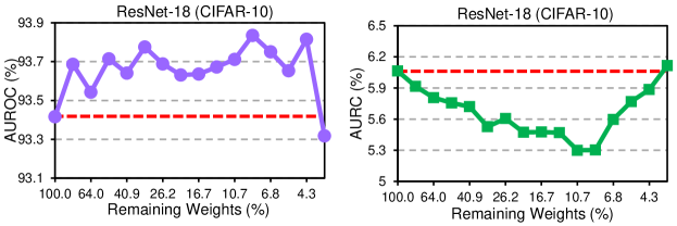
Figure 11: Evaluation of misclassified examples detection under two metrics: AUROC and AURC. Backbone is ResNet-18 [15].

6 Conclusion

In this work, we investigate the chaotic behavior of OOD detection along the optimization trajectory during training, which is ignored by previous studies. We find OOD detection suffers from instability and overfitting, and verify that AoP, consisting of model averaging and pruning, can eliminate such two drawbacks. Model average smooth the weights of models, contributing to a stable performance of the final checkpoint. Pruning increases the sparsity of the model, evading learning too many common features. We also provide a theoretical analysis of the connection between sparsity and OOD detection. The comprehensive experiments verify that AoP achieves great improvement on OOD detection.

Supplementary Material:

Average of Pruning: Improving Performance and Stability of Out-of-Distribution Detection

This appendix can be divided into 6 parts. To be precise,

• In Section A, we give detailed descriptions of the OOD datasets.

• In Section B, we give some details about the evaluation metrics used in the main text.

• In Section C, we present the proofs of the theorems in the main text.

• In Section D, we show the experimental configurations in detail.

• In Section E, we provide some additional experimental results that we omit in the main body of the paper because of the limitation in space.

• In Section F, we provide some discussions about our work.

Appendix A Dataset Details

We would like to introduce the OOD datasets used in the paper.

• Textures [3] is an evolving collection of textural images in the wild, consisting of 5640 images, organized into 47 items.

• SVHN [36] contains 10 classes comprised of the digits 0-9 in street view, which contains 26,032 images for testing.

• Place365 [54] consists in 1,803,460 large-scale photographs of scenes. Each photograph belongs to one of 365 classes. Following the work of [17, 33], we use a subset of Place365 as OOD data.

• LSUN [51] has a test set of 10,000 images of 10 different scene categories. Following [31, 33], we construct two datasets, LSUN-crop and LSUN-resize, by randomly cropped and downsampling LSUN test set, respectively.

• iSUN [49] is a ground truth of gaze traces on images from the SUN dataset. The dataset contains 2,000 images for the test.

Appendix B Evaluation Metrics

We would like to introduce the metrics applied in the main text.

B.1 Metrics in out-of-distribution detection

• AUROC measures the Area Under the Receiver Operating Characteristic curve (AUROC). The ROC curve depicts the relationship between True Positive Rate and False Positive Rate.

• AUPR is the Area under the Precision-Recall (PR) curve. The PR curve is a graph showing the precision=TP/(TP+FP) versus recall=TP/(TP+FN). AUPR typically regards the in-distribution samples as positive samples.

• FPR-95%-TPR (FPR95) can be interpreted as the probability that a negative (OOD data) sample is classified as an in-distribution prediction when the true positive rate (TPR) is as high as 95%. We denote it as FPR95 for short.

B.2 Metrics in misclassification detection

The metrics of AUROC and FPR95 have been introduced in the previous part, so we give descriptions of the remaining metrics: AURC, E-AURC, and AUPR-Err. The difference of AUROC and FPR95 in OOD detection and misclassification detection is that the former regards OOD data as negatives while the latter regards misclassified examples as negatives.

• AURC is the area under the risk-coverage curve. Risk-coverage curve is defined by the work of [geifman2018biasreduced].

• E-AURC, known as excess AURC, is a normalization of AURC where we subtract the AURC of the best score function in hindsight [geifman2018biasreduced].

• AUPR-Err is the Area under the Precision-Recall (PR) curve. The PR curve is a graph showing the precision versus recall. The metric AUPR-Err indicates the area under the precision-recall curve where errors are specified as positives, since we want to detect misclassified examples.

Appendix C Proofs

C.1 Proof for Theorem 1

Theorem C.1.

Suppose the distributions of ID and OOD data follow Gaussian distribution in Eq. (2), then $\mathcal{R}_{\mathrm{ID}}\left(f_{\mathrm{Bayes}}\right)$ and $\mathcal{R}_{\mathrm{OOD}}\left(f_{\mathrm{Bayes}}\right)$ could be simplified to

$$\mathcal{R}_{\mathrm{ID}}\left(f_{\mathrm{Bayes}}\right)=\,\,\mathrm{Pr}\left\{\mathcal{N}\left(0,1\right)>\frac{\sqrt{1+d\eta^{2}}}{\sigma}\right\},$$

$$\mathcal{R}_{\mathrm{OOD}}\left(f_{\mathrm{Bayes}}\right)=\mathrm{Pr}\left\{\mathcal{N}\left(0,1\right)>\frac{\delta-d\eta^{2}}{\sigma\cdot\sqrt{1+d\eta^{2}}}\right\}+\mathrm{Pr}\left\{\mathcal{N}\left(0,1\right)>\frac{\delta+d\eta^{2}}{\sigma\cdot\sqrt{1+d\eta^{2}}}\right\}.$$

Proof. Under the assumption of distribution for ID and OOD data in Eq. (2), the decision is based on the sign of logits from Bayes classifier:

$$f_{\mathrm{Bayes}}\left(\boldsymbol{x}\right)=x_{1}+\eta\sum_{i=2}^{d+1}{x_{i}}.$$

The in-distribution classification risk of $f_{\mathrm{Bayes}}$, i.e., $\mathcal{R}_{\mathrm{ID}}\left(f_{\mathrm{Bayes}}\right)$, is

$$\mathcal{R}_{\mathrm{ID}}\left(f_{\mathrm{Bayes}}\right) =\underset{\left(\boldsymbol{x},y\right)\in\mathcal{D}_{\mathrm{ID}}}{\mathrm{Pr}}\left\{\mathrm{sign}\left(f\left(\boldsymbol{x}\right)\right)\neq y\right\}$$

$$=\underset{\left(\boldsymbol{x},y\right)\in\mathcal{D}_{\mathrm{ID}}}{\mathrm{Pr}}\left\{y\cdot\left(\mathcal{N}\left(y,\sigma^{2}\right)+\sum_{i=2}^{d+1}{\eta\mathcal{N}\left(y\eta,\sigma^{2}\right)}\right)<0\right\}$$

$$=\underset{\left(\boldsymbol{x},y\right)\in\mathcal{D}_{\mathrm{ID}}}{\mathrm{Pr}}\left\{\mathcal{N}\left(1,\sigma^{2}\right)+\sum_{i=2}^{d+1}{\eta\mathcal{N}\left(\eta,\sigma^{2}\right)<0}\right\}$$

$$=\underset{\left(\boldsymbol{x},y\right)\in\mathcal{D}_{\mathrm{ID}}}{\mathrm{Pr}}\left\{\mathcal{N}\left(1+d\eta^{2},\left(1+d\eta^{2}\right)\sigma^{2}\right)<0\right\}$$

$$=\mathrm{Pr}\left\{\mathcal{N}\left(0,1\right)>\frac{\sqrt{1+d\eta^{2}}}{\sigma}\right\}.$$

The out-of-distribution rejection risk of $f_{\mathrm{Bayes}}$, i.e., $\mathcal{R}_{\mathrm{OOD}}\left(f_{\mathrm{Bayes}}\right)$, is

$$\mathcal{R}_{\mathrm{OOD}}\left(f_{\mathrm{Bayes}}\right) =\underset{\left(\boldsymbol{x},q\right)\in\mathcal{D}_{\mathrm{OOD}}}{\mathrm{Pr}}\left\{\left|f\left(\boldsymbol{x}\right)\right|>\delta\right\}$$

$$=\underset{\left(\boldsymbol{x},q\right)\in\mathcal{D}_{\mathrm{OOD}}}{\mathrm{Pr}}\left\{\left(\mathcal{N}\left(0,\sigma^{2}\right)+\sum_{i=2}^{d+1}{\eta\mathcal{N}\left(\eta,\sigma^{2}\right)}\right)>\delta\right\}$$

$$\quad\quad\quad+\underset{\left(\boldsymbol{x},q\right)\in\mathcal{D}_{\mathrm{OOD}}}{\mathrm{Pr}}\left\{\left(\mathcal{N}\left(0,\sigma^{2}\right)+\sum_{i=2}^{d+1}{\eta\mathcal{N}\left(\eta,\sigma^{2}\right)}\right)<-\delta\right\}\,\,$$

$$=\underset{\left(\boldsymbol{x},q\right)\in\mathcal{D}_{\mathrm{OOD}}}{\mathrm{Pr}}\left\{\mathcal{N}\left(d\eta^{2},\left(1+d\eta^{2}\right)\sigma^{2}\right)>\delta\right\}$$

$$\quad\quad\quad+\underset{\left(\boldsymbol{x},q\right)\in\mathcal{D}_{\mathrm{OOD}}}{\mathrm{Pr}}\left\{\mathcal{N}\left(d\eta^{2},\left(1+d\eta^{2}\right)\sigma^{2}\right)<-\delta\right\}$$

$$=\mathrm{Pr}\left\{\mathcal{N}\left(0,1\right)>\frac{\delta-d\eta^{2}}{\sigma\sqrt{1+d\eta^{2}}}\right\}+\mathrm{Pr}\left\{\mathcal{N}\left(0,1\right)>\frac{\delta+d\eta^{2}}{\sigma\sqrt{1+d\eta^{2}}}\right\}.$$

C.2 Proof for Theorem 2

Theorem C.2.

The classifier $f_{\mathrm{LASSO}}$ [14] obtained by minimizing the loss in Eq. (6) is

$$f_{\mathrm{LASSO}}\left(\boldsymbol{x}\right)=\left(\left(1-\lambda\right)_{+}\cdot x_{1}+\sum_{i=2}^{d+1}{\left(\eta-\lambda\right)_{+}\cdot x_{i}}\right),$$

where $\left(\cdot\right)_{+}$ means the positive part of a number.

Proof. Taking the derivative of loss with LASSO [14] in Eq. (6) with respect to $\boldsymbol{w}$ and setting equal to 0 gives

$$\mathbb{E}_{\left(\boldsymbol{x},y\right)\sim\mathcal{D}_{\mathrm{ID}}}\left\{-\frac{\boldsymbol{x}}{\sigma}\left(y-\frac{\boldsymbol{x}^{\mathrm{T}}\boldsymbol{w}}{\sigma}\right)+\lambda\cdot\mathrm{sign}\left(\boldsymbol{w}\right)\right\}=0.$$

Considering the distribution of ID data, then $\mathbb{E}_{\left(\boldsymbol{x},y\right)\sim\mathcal{D}_{\mathrm{ID}}}\frac{\boldsymbol{xx}^{\mathrm{T}}}{\sigma^{2}}=I$, and $\mathbb{E}_{\left(\boldsymbol{x},y\right)\sim\mathcal{D}_{\mathrm{ID}}}\left(\frac{\boldsymbol{x}y}{\sigma}\right)=\left[1,\eta,\dots,\eta\right]^{\mathrm{T}}$. Then, we could get the solution of LASSO as follows

$$\boldsymbol{w}_{\mathrm{LASSO}} =\mathbb{E}_{\left(\boldsymbol{x},y\right)\sim\mathcal{D}_{\mathrm{ID}}}\left\{\frac{\boldsymbol{x}y}{\sigma}-\lambda\cdot\mathrm{sign}\left(\boldsymbol{w}_{\mathrm{LASSO}}\right)\right\}$$

$$=\left[1,\eta,\cdots,\eta\right]^{\mathrm{T}}-\lambda\cdot\mathrm{sign}\left(\boldsymbol{w}_{\mathrm{LASSO}}\right)$$

$$=\left[\left(1-\lambda\right)_{+},\left(\eta-\lambda\right)_{+},\cdots,\left(\eta-\lambda\right)_{+}\right]^{\mathrm{T}}.$$

Thus, the output of LASSO is as follows

$$f_{\mathrm{LASSO}}\left(\boldsymbol{x}\right)=\boldsymbol{w}_{\mathrm{LASSO}}^{\mathrm{T}}\boldsymbol{x}=\left(1-\lambda\right)_{+}\cdot x_{1}+\sum_{i=2}^{d+1}{\left(\eta-\lambda\right)_{+}\cdot x_{i}}.$$

More detailed results about the solution of LASSO could be found in Section 3.4 from the textbook [14].

Appendix D Experimental Configurations

D.1 Experimental settings on CIFAR benchmarks

We would like to add some details about the settings of AoP on CIFAR benchmarks. For model averaging, we set the started epoch of the model averaging $t_{0}$ to 100. For pruning (i.e., LTH with weight rewinding [11]), we prune 20% of the weights in each pruning stage and repeat 9 times (reaching a sparsity of 86.3%). To show the influence of sparsity on OOD detection, we continue to prune the model 15 times, and draw the curve between sparsity and performance of OOD detection.

D.2 Experimental settings of other OOD detection methods

The OOD detection methods compared in the main text include MSP [16], ODIN [31], Mahalanobis distance [29], energy score [33], GradNorm [21], ReAct [42], MaxLogit [18], VOS [6], KNN [43], and ViM [47]. Most of our settings refer to the work of OpenOOD [50] and their original codes.

For ODIN [31], we set the temperature scaling $T$ to 1000. For Mahalanobis distance [29], we set the magnitude of noise to 0.005. For energy score, we set the temperature scaling $T$ to 1. For ReAct [42], we set the rectification percentile to 90. For KNN [43], we set $k$ to 50. For ViM [47], we set the dimension of principle space to 256.

Appendix E Additional Experimental Results

We would like to provide more experimental results which are not included in the main text because of the limit in space. We provide more curves about the phenomenon of instability and overfitting that we find in the paper.

E.1 Experiments about instability and overfitting

The phenomenon of instability and overfitting exists in different OOD datasets. In the main text, we show that the curve of the model trained on CIFAR-10 and tested on LSUN-R [51]. The curves of testing on other OOD datasets are shown in Fig. 12. Due to the limit of space, we show the curve of AUROC in the main text. We also show how AUPR and FPR95 vary during the training stage, and the results are shown in Fig. 13. It reveals instability and overfitting exist in various metrics.

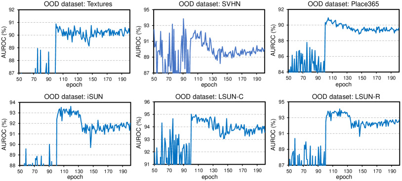
Figure 12: Instability and overfitting occur in various OOD datasets. The model is ResNet-18 [15] trained on CIFAR-10. The OOD datasets include Textures [3], SVHN [36], Place365 [54], iSUN [49], LSUN-C [51], and LSUN-R [51]. The OOD datasets are indicated in the title of each figure. The results show that instability and overfitting exist in different OOD datasets.

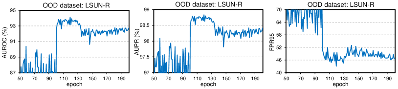
Figure 13: Different metrics (AUROC, AUPR, and FPR95) in OOD detection show instability and overfitting. The model is ResNet-18 [15] trained on CIFAR-10. The OOD dataset used is LSUN-R [51].

The phenomenon of instability and overfitting occurs in different networks. We show that instability and overfitting also exist in other networks, like WideResNet-28-10 [52], and the curves are presented in Fig. 14.

Figure 14: Instability and overfitting occur in other network. The model is WideResNet-28-10 [52] trained on CIFAR-10. The OOD datasets include Textures [3], SVHN [36], Place365 [54], iSUN [49], LSUN-C [51], and LSUN-R [51]. The OOD datasets are indicated in the title of each figure.

E.2 Results of AoP on other networks

OOD detection. We conduct more experiments on other networks to verify that AoP promotes OOD detection, including Vgg-16 [41], WideResNet-40-2 [52] and MobileNet [19]. The results are listed in Tab. 9. As shown in the results, AoP achieves consistent improvement in OOD detection.

Table 9: Performance of OOD detection for other networks. The models are trained on CIFAR-10. The testing OOD datasets are the same as CIFAR benchmarks in the main text. The best results are boldfaced for highlighting.

Method	Vgg-16			WRN-40-2			MobileNet
	AUROC $\uparrow$	AUPR $\uparrow$	FPR $\downarrow$	AUROC $\uparrow$	AUPR $\downarrow$	FPR $\downarrow$	AUROC $\uparrow$	AUPR $\uparrow$	FPR $\downarrow$
MSP	88.88	97.51	59.22	89.20	97.87	59.88	88.05	97.61	61.96
+ AoP	89.88	97.70	56.63	90.24	98.14	57.25	89.93	98.21	58.96

Misclassification detection. We conduct more experiments on other networks to verify that AoP promotes misclassification detection, including Vgg-16 [41], and ResNet-18 [15]. The results are listed in Tab. 10.

Table 10: Performance of misclassification detection for more datasets and networks. AURC and E-AURC values are multiplied by $10^{3}$. Other values are percentages. The best results are boldfaced for highlighting.

Model	Method	CIFAR-10					CIFAR-100
		AUROC $\uparrow$	AURC $\downarrow$	E-AURC $\downarrow$	AUPR-Err $\uparrow$	FPR95 $\downarrow$	AUROC $\uparrow$	AURC $\downarrow$	E-AURC $\downarrow$	AUPR-Err $\uparrow$	FPR95 $\downarrow$
Vgg-16	MSP	91.04	10.36	7.97	44.63	45.60	85.91	91.12	47.21	67.70	66.06
	+ AoP	91.47	9.45	7.31	45.25	41.40	86.51	86.23	42.74	67.99	64.93
ResNet-18	MSP	93.41	6.06	4.32	45.88	39.02	86.03	84.75	43.31	66.29	66.53
	+ AoP	93.77	5.52	3.90	45.59	37.17	86.25	81.76	42.06	66.42	65.98

Appendix F Discussions

In this paper, we show that the performance of OOD detection suffers from instability and overfitting in the training stage. Our findings reveal that the training dynamics provide an interesting research perspective ignored by previous studies in the field of OOD detection. The method is this paper is very simple and effective.

We use model averaging to stabilize the performance of OOD detection in training. The realization is convenient and has almost no computational overhead. We adopt LTH [10, 11] as the pruning method, which is a very well-known method for post-training pruning. LTH has detailed implementation codes and is easy to reproduce the results. Besides, its realization is consistent with our theoretical motivation from LASSO, which could certify our theoretical results. We have also verified that various during-training pruning methods like GMP [55], RigL [7], and GraNet [32] could improve the performance of OOD detection, which are often more efficient. Various pruning techniques could achieve improvement in OOD detection rather than just LTH. Comprehensive experiments in the paper verify the effectiveness of pruning in OOD detection.

References

- Bitterwolf et al. [2022] Julian Bitterwolf, Alexander Meinke, Maximilian Augustin, and Matthias Hein. Breaking down out-of-distribution detection: Many methods based on ood training data estimate a combination of the same core quantities. In International Conference on Machine Learning, pages 2041–2074. PMLR, 2022.
- Chaudhari et al. [2017] Pratik Chaudhari, Anna Choromanska, Stefano Soatto, Yann LeCun, Carlo Baldassi, Christian Borgs, Jennifer Chayes, Levent Sagun, and Riccardo Zecchina. Entropy-SGD: Biasing gradient descent into wide valleys. In International Conference on Learning Representations, 2017.
- Cimpoi et al. [2014] Mircea Cimpoi, Subhransu Maji, Iasonas Kokkinos, Sammy Mohamed, and Andrea Vedaldi. Describing textures in the wild. In Proceedings of the IEEE conference on computer vision and pattern recognition, pages 3606–3613, 2014.
- Deng et al. [2009] Jia Deng, Wei Dong, Richard Socher, Li-Jia Li, Kai Li, and Li Fei-Fei. Imagenet: A large-scale hierarchical image database. In 2009 IEEE conference on computer vision and pattern recognition, pages 248–255. Ieee, 2009.
- Dosovitskiy et al. [2021] Alexey Dosovitskiy, Lucas Beyer, Alexander Kolesnikov, Dirk Weissenborn, Xiaohua Zhai, Thomas Unterthiner, Mostafa Dehghani, Matthias Minderer, Georg Heigold, Sylvain Gelly, Jakob Uszkoreit, and Neil Houlsby. An image is worth 16x16 words: Transformers for image recognition at scale. In International Conference on Learning Representations, 2021.
- Du et al. [2022] Xuefeng Du, Zhaoning Wang, Mu Cai, and Sharon Li. Towards unknown-aware learning with virtual outlier synthesis. In International Conference on Learning Representations, 2022.
- Evci et al. [2020] Utku Evci, Trevor Gale, Jacob Menick, Pablo Samuel Castro, and Erich Elsen. Rigging the lottery: Making all tickets winners. In International Conference on Machine Learning, pages 2943–2952. PMLR, 2020.
- Filos et al. [2020] Angelos Filos, Panagiotis Tigkas, Rowan McAllister, Nicholas Rhinehart, Sergey Levine, and Yarin Gal. Can autonomous vehicles identify, recover from, and adapt to distribution shifts? In International Conference on Machine Learning, pages 3145–3153. PMLR, 2020.
- Fort et al. [2021] Stanislav Fort, Jie Ren, and Balaji Lakshminarayanan. Exploring the limits of out-of-distribution detection. Advances in Neural Information Processing Systems, 34, 2021.
- Frankle and Carbin [2019] Jonathan Frankle and Michael Carbin. The lottery ticket hypothesis: Finding sparse, trainable neural networks. In International Conference on Learning Representations, 2019.
- Frankle et al. [2020] Jonathan Frankle, Gintare Karolina Dziugaite, Daniel Roy, and Michael Carbin. Linear mode connectivity and the lottery ticket hypothesis. In International Conference on Machine Learning, pages 3259–3269. PMLR, 2020.
- Garipov et al. [2018] Timur Garipov, Pavel Izmailov, Dmitrii Podoprikhin, Dmitry P Vetrov, and Andrew G Wilson. Loss surfaces, mode connectivity, and fast ensembling of dnns. Advances in neural information processing systems, 31, 2018.
- Han et al. [2015] Song Han, Jeff Pool, John Tran, and William Dally. Learning both weights and connections for efficient neural network. In Advances in Neural Information Processing Systems, volume 28, 2015.
- Hastie et al. [2009] Trevor Hastie, Robert Tibshirani, Jerome H Friedman, and Jerome H Friedman. The elements of statistical learning: data mining, inference, and prediction, volume 2. Springer, 2009.
- He et al. [2016] Kaiming He, Xiangyu Zhang, Shaoqing Ren, and Jian Sun. Deep residual learning for image recognition. In Proceedings of the IEEE conference on Computer Vision and Pattern Recognition, pages 770–778, 2016.
- Hendrycks and Gimpel [2017] Dan Hendrycks and Kevin Gimpel. A baseline for detecting misclassified and out-of-distribution examples in neural networks. In International Conference on Learning Representations, 2017.
- Hendrycks et al. [2019] Dan Hendrycks, Mantas Mazeika, and Thomas Dietterich. Deep anomaly detection with outlier exposure. In International Conference on Learning Representations, 2019.
- Hendrycks et al. [2022] Dan Hendrycks, Steven Basart, Mantas Mazeika, Andy Zou, Joseph Kwon, Mohammadreza Mostajabi, Jacob Steinhardt, and Dawn Song. Scaling out-of-distribution detection for real-world settings. 2022.
- Howard et al. [2017] Andrew G Howard, Menglong Zhu, Bo Chen, Dmitry Kalenichenko, Weijun Wang, Tobias Weyand, Marco Andreetto, and Hartwig Adam. Mobilenets: Efficient convolutional neural networks for mobile vision applications. arXiv preprint arXiv:1704.04861, 2017.
- Huang and Li [2021] Rui Huang and Yixuan Li. Mos: Towards scaling out-of-distribution detection for large semantic space. In Proceedings of the IEEE/CVF Conference on Computer Vision and Pattern Recognition, pages 8710–8719, 2021.
- Huang et al. [2021] Rui Huang, Andrew Geng, and Yixuan Li. On the importance of gradients for detecting distributional shifts in the wild. Advances in Neural Information Processing Systems, 34:677–689, 2021.
- Ilyas et al. [2019] Andrew Ilyas, Shibani Santurkar, Logan Engstrom, Brandon Tran, and Aleksander Madry. Adversarial examples are not bugs, they are features. In Advances in Neural Information Processing Systems, 2019.
- Izmailov et al. [2018] P Izmailov, AG Wilson, D Podoprikhin, D Vetrov, and T Garipov. Averaging weights leads to wider optima and better generalization. In 34th Conference on Uncertainty in Artificial Intelligence 2018, UAI 2018, pages 876–885, 2018.
- Jain et al. [2018] Prateek Jain, Sham Kakade, Rahul Kidambi, Praneeth Netrapalli, and Aaron Sidford. Parallelizing stochastic gradient descent for least squares regression: mini-batching, averaging, and model misspecification. Journal of Machine Learning Research, 18, 2018.
- Krizhevsky et al. [2009] Alex Krizhevsky et al. Learning multiple layers of features from tiny images. 2009.
- Lakshminarayanan et al. [2017] Balaji Lakshminarayanan, Alexander Pritzel, and Charles Blundell. Simple and scalable predictive uncertainty estimation using deep ensembles. Advances in neural information processing systems, 30, 2017.
- LeCun et al. [1989] Yann LeCun, John Denker, and Sara Solla. Optimal brain damage. Advances in neural information processing systems, 2, 1989.
- Lee et al. [2018a] Kimin Lee, Honglak Lee, Kibok Lee, and Jinwoo Shin. Training confidence-calibrated classifiers for detecting out-of-distribution samples. In International Conference on Learning Representations, 2018a.
- Lee et al. [2018b] Kimin Lee, Kibok Lee, Honglak Lee, and Jinwoo Shin. A simple unified framework for detecting out-of-distribution samples and adversarial attacks. Advances in neural information processing systems, 31, 2018b.
- Li et al. [2018] Hao Li, Zheng Xu, Gavin Taylor, Christoph Studer, and Tom Goldstein. Visualizing the loss landscape of neural nets. Advances in neural information processing systems, 31, 2018.
- Liang et al. [2018] Shiyu Liang, Yixuan Li, and R Srikant. Enhancing the reliability of out-of-distribution image detection in neural networks. In International Conference on Learning Representations, 2018.
- Liu et al. [2021] Shiwei Liu, Tianlong Chen, Xiaohan Chen, Zahra Atashgahi, Lu Yin, Huanyu Kou, Li Shen, Mykola Pechenizkiy, Zhangyang Wang, and Decebal Constantin Mocanu. Sparse training via boosting pruning plasticity with neuroregeneration. Advances in Neural Information Processing Systems, 34:9908–9922, 2021.
- Liu et al. [2020] Weitang Liu, Xiaoyun Wang, John Owens, and Yixuan Li. Energy-based out-of-distribution detection. Advances in Neural Information Processing Systems, 33:21464–21475, 2020.
- Ming et al. [2022] Yifei Ming, Ying Fan, and Yixuan Li. POEM: Out-of-distribution detection with posterior sampling. In Proceedings of the 39th International Conference on Machine Learning, Proceedings of Machine Learning Research. PMLR, 2022.
- Moon et al. [2020] Jooyoung Moon, Jihyo Kim, Younghak Shin, and Sangheum Hwang. Confidence-aware learning for deep neural networks. In international conference on machine learning, pages 7034–7044. PMLR, 2020.
- Netzer et al. [2011] Yuval Netzer, Tao Wang, Adam Coates, Alessandro Bissacco, Bo Wu, and Andrew Y Ng. Reading digits in natural images with unsupervised feature learning. 2011.
- Neu and Rosasco [2018] Gergely Neu and Lorenzo Rosasco. Iterate averaging as regularization for stochastic gradient descent. In Conference On Learning Theory, pages 3222–3242. PMLR, 2018.
- Nguyen et al. [2015] Anh M Nguyen, Jason Yosinski, and Jeff Clune. Deep neural networks are easily fooled: High confidence predictions for unrecognizable images. 2015 IEEE Conference on Computer Vision and Pattern Recognition (CVPR), pages 427–436, 2015.
- Ren et al. [2019] Jie Ren, Peter J Liu, Emily Fertig, Jasper Snoek, Ryan Poplin, Mark Depristo, Joshua Dillon, and Balaji Lakshminarayanan. Likelihood ratios for out-of-distribution detection. Advances in neural information processing systems, 32, 2019.
- Salehi et al. [2021] Mohammadreza Salehi, Hossein Mirzaei, Dan Hendrycks, Yixuan Li, Mohammad Hossein Rohban, and Mohammad Sabokrou. A unified survey on anomaly, novelty, open-set, and out-of-distribution detection: Solutions and future challenges. arXiv preprint arXiv:2110.14051, 2021.
- Simonyan and Zisserman [2014] Karen Simonyan and Andrew Zisserman. Very deep convolutional networks for large-scale image recognition. arXiv preprint arXiv:1409.1556, 2014.
- Sun et al. [2021] Yiyou Sun, Chuan Guo, and Yixuan Li. React: Out-of-distribution detection with rectified activations. Advances in Neural Information Processing Systems, 34, 2021.
- Sun et al. [2022] Yiyou Sun, Yifei Ming, Xiaojin Zhu, and Yixuan Li. Out-of-distribution detection with deep nearest neighbors. 2022.
- Tao et al. [2021] Lue Tao, Lei Feng, Jinfeng Yi, Sheng-Jun Huang, and Songcan Chen. Better safe than sorry: Preventing delusive adversaries with adversarial training. In Advances in Neural Information Processing Systems, 2021.
- Tao et al. [2022] Lue Tao, Lei Feng, Hongxin Wei, Jinfeng Yi, Sheng-Jun Huang, and Songcan Chen. Can adversarial training be manipulated by non-robust features? In Advances in Neural Information Processing Systems, 2022.
- Tibshirani [1996] Robert Tibshirani. Regression shrinkage and selection via the lasso. Journal of the Royal Statistical Society: Series B (Methodological), 58(1):267–288, 1996.
- Wang et al. [2022] Haoqi Wang, Zhizhong Li, Litong Feng, and Wayne Zhang. Vim: Out-of-distribution with virtual-logit matching. In Proceedings of the IEEE/CVF Conference on Computer Vision and Pattern Recognition, pages 4921–4930, 2022.
- Wei et al. [2022] Hongxin Wei, Renchunzi Xie, Hao Cheng, Lei Feng, Bo An, and Yixuan Li. Mitigating neural network overconfidence with logit normalization. 2022.
- Xu et al. [2015] Pingmei Xu, Krista A Ehinger, Yinda Zhang, Adam Finkelstein, Sanjeev R Kulkarni, and Jianxiong Xiao. Turkergaze: Crowdsourcing saliency with webcam based eye tracking. arXiv preprint arXiv:1504.06755, 2015.
- Yang et al. [2022] Jingkang Yang, Pengyun Wang, Dejian Zou, Zitang Zhou, Kunyuan Ding, Wenxuan Peng, Haoqi Wang, Guangyao Chen, Bo Li, Yiyou Sun, Xuefeng Du, Kaiyang Zhou, Wayne Zhang, Dan Hendrycks, Yixuan Li, and Ziwei Liu. Openood: Benchmarking generalized out-of-distribution detection, 2022.
- Yu et al. [2015] Fisher Yu, Ari Seff, Yinda Zhang, Shuran Song, Thomas Funkhouser, and Jianxiong Xiao. Lsun: Construction of a large-scale image dataset using deep learning with humans in the loop. arXiv preprint arXiv:1506.03365, 2015.
- Zagoruyko and Komodakis [2016] Sergey Zagoruyko and Nikos Komodakis. Wide residual networks. In Proceedings of the British Machine Vision Conference (BMVC), 2016.
- Zhang et al. [2017] Chiyuan Zhang, Samy Bengio, Moritz Hardt, Benjamin Recht, and Oriol Vinyals. Understanding deep learning requires rethinking generalization. In International Conference on Learning Representations, 2017.
- Zhou et al. [2017] Bolei Zhou, Agata Lapedriza, Aditya Khosla, Aude Oliva, and Antonio Torralba. Places: A 10 million image database for scene recognition. IEEE transactions on pattern analysis and machine intelligence, 40(6):1452–1464, 2017.
- Zhu and Gupta [2017] Michael Zhu and Suyog Gupta. To prune, or not to prune: exploring the efficacy of pruning for model compression. arXiv preprint arXiv:1710.01878, 2017.