Using vibrating wire in non-linear regime as a thermometer in superfluid ³He-B

Abstract

Vibrating wires are common temperature probes in ³He experiments. By measuring mechanical resonance of a wire driven by AC current in magnetic field one can directly obtain temperature-dependent viscous damping. This is easy to do in a linear regime where wire velocity is small enough and damping force is proportional to velocity. At lowest temperatures in superfluid ³He-B a strong non-linear damping appears and linear regime shrinks to a very small velocity range. Expanding measurements to the non-linear area can significantly improve sensitivity. In this note I describe some technical details useful for analyzing such temperature measurements.

Vibrating wire in the linear regime

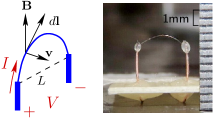
Figure 1: Wire loop driven by current in magnetic field. On the right image of a real device is shown (wire thickness $d=13\,\mu$m, wire projection length $L=2.7\,$mm).

First consider a wire loop with current $I$ moving in magnetic field $\bf B$ with velocity ${\bf v}\perp{\bf B}$. Geometry of this system is shown on Fig 1. Force $d{\bf F}$ acting on a piece of wire $d{\bf l}$ and EMF voltage $dV$ across it are

$$d{\bf F}=I\,[d{\bf l}\times{\bf B}],\qquad dV={\bf v}\cdot[d{\bf l}\times{\bf B}],$$ (1)

where positive direction of current is along $d{\bf l}$ and positive voltage produces current in the same direction (thus potential is decreasing along $d{\bf l}$). By integrating along the wire one can find total force and voltage:

$$F=ILB,\qquad V=vLB,$$ (2)

where $L$ is projection of the wire loop to a plane perpendicular to magnetic field and $v$ is mean velocity along the wire length. Also from (1) one can find mechanical power produced by the force:

$$W=\int{\bf v}\cdot d{\bf F}=I\,V.$$ (3)

In the linear regime the wire driven by AC current can be represented as a linear oscillator:

$$\ddot{x}=-\omega^{2}_{0}x-\delta\dot{x}+\gamma\,\cos\omega t,\qquad\gamma=ILB/m_{w}$$ (4)

where $x$ is average displacement, average velocity $v=\dot{x}$, and parameters $m_{w}$, $\omega_{0}$, $\delta$ are effective mass of the wire, resonance frequency, and resonance width. $\gamma$ is force divided by mass $m_{w}$.

Non-linear regime in superfluid ³He-B

Behaviour of a vibrating wire in superfluid ³He-B at low temperatures was investigated long time ago in Lancaster [1, 2, 3]. There is a threshold velocity at which wire can emit quasiparticles and dissipate extra energy. This threshold is called ”pair-breaking velocity”, it is some fraction of Landau velocity $\Delta/p_{F}$, usually 1/3 or smaller depending on wire geometry. At zero pressure and low temperatures typical value is less then 10 mm/s. Below the pair-breaking velocity damping is determined by quasiparticle scattering, this is the non-linear regime we are interested in. Force $F_{v}$ acting on a wire moving with velocity $v$ has been derived by applying spectrum of Bogolubov quasiparticles to some scattering model. There are a few results: for a simple 1D model, for specular and diffusive 3D scattering. At the moment we are not interested in exact expression, but there is an important result that the force can be written via a temperature-independent function $\gamma_{v}$ of reduced velocity $v/v_{0}$:

$$F_{v}(\dot{x})=-m_{w}\delta_{0}v_{0}\gamma_{v}\left(\frac{v}{v_{0}}\right),$$ (5)

where temperature-dependent parameters $\delta_{0}$ and $v_{0}$ are

$$\delta_{0}=\frac{p_{F}^{2}v_{F}N(0)}{\rho_{w}\,d}\exp\left(-\frac{\Delta}{kT}\right),\qquad v_{0}=\frac{kT}{p_{F}},$$ (6)

$p_{F}$, $v_{F}$, $N(0)$ are ³He Fermi momentum, Fermi velocity, and density of states at Fermi level, $\Delta$ is superfluid gap, $\rho_{w}$ and $d$ are density and diameter of the wire. Asymptotic behaviour of function $\gamma_{v}$ at small velocity ($v\ll v_{0}$) should be linear, which corresponds to the linear regime: $F_{v}(\dot{x})=-m_{w}\delta_{0}vs_{0}$ with some temperature-independent dimensionless calibration factor $s_{0}$. We also assume that function $\gamma_{v}$ is already averaged along the wire loop and written for the average velocity $v$.

Now the equation of motion is:

$$\ddot{x}=-\omega_{0}^{2}x-\delta_{i}\dot{x}-\delta_{0}v_{0}\gamma_{v}\left(\frac{\dot{x}}{v_{0}}\right)+\gamma\cos\omega t,$$ (7)

where intrinsic damping of the wire is called $\delta_{i}$ and damping caused by interaction with helium is described by the term with $\gamma_{v}$.

To find response at frequency $\omega$ we rewrite the equation of motion in van der Pol coordinates:

$$u=x\cos\omega t-\frac{\dot{x}}{\omega}\sin\omega t,\qquad v=-x\sin\omega t-\frac{\dot{x}}{\omega}\cos\omega t.$$ (8)

and average over period $0<\omega t<2\pi$. During this calculation we need to average function $\gamma_{v}(\dot{x}/v_{0})$ multiplied by $\sin\omega t$ and $\cos\omega t$. This can be done by making substitution

$$u\,\omega/v_{0}=c\cos\phi,\qquad v\,\omega/v_{0}=c\sin\phi,$$ (9)

shifting averaging period by $\phi$, and obtaining integrals with one parameter $c$:

$$\langle\gamma_{v}(\dot{x}/v_{0})\sin\omega t\rangle=\langle\gamma_{v}(-u\,\omega/v_{0}\sin\omega t-v\,\omega/v_{0}\cos\omega t)\sin\omega t\rangle=$$ (10)

$$= u\frac{\omega}{cv_{0}}\int_{0}^{2\pi}\gamma_{v}(-c\sin\omega t)\,\sin\omega t\,\frac{d\omega t}{2\pi}=-\frac{u}{2}\frac{\omega}{v_{0}}S(c),$$ (11)

and similarly

$$\langle\gamma_{v}(\dot{x}/v_{0})\cos\omega t\rangle=-\frac{v}{2}\frac{\omega}{v_{0}}S(c)$$ (12)

where we introduce function $S(c)$ of positive dimensionless argument $c=\frac{\omega}{v_{0}}\sqrt{u^{2}+v^{2}}$ as

$$S(c)=-\frac{2}{c}\int_{0}^{2\pi}\gamma_{v}(-c\sin\omega t)\,\sin\omega t\,\frac{d\omega t}{2\pi}$$ (13)

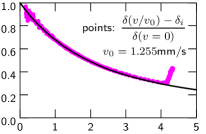
Figure 2: Solid line: analytical function $S(c)$ for 1D scattering model (15). Points: an example of experimental data scaled by choosing $v_{0}=1.255$ mm/s (see Fig. 3 and (23) for details). Deviation at $c>4$ is the pair-breaking regime.

If function $\gamma_{v}$ is known then function $S$ can be calculated analytically or numerically. Normally only a limited range of reduced velocities is needed and $S$ can be easily tabulated or approximated by some smooth function. For example, if damping is linear, $\gamma_{v}(x)=x$ then $S(c)=1$. For 1D scattering model [1] $S$ can be written via special functions:

$$\gamma_{v}(x) = \mbox{sign}(x)(1-\exp(-|x|)),$$ (14)

$$S(c) = \frac{2}{c}\left(I_{1}(c)-L_{-1}(c)+\frac{2}{\pi}\right),$$ (15)

where $I_{n}(x)$ is modified Bessel function of first kind and $L_{n}(x)$ is modified Struve function. For an arbitrary expansion

$$\gamma_{v}(x) = a_{1}x+\mbox{sign}(x)\,a_{2}x^{2}+a_{3}x^{3}+\mbox{sign}(x)\,a_{4}x^{3},$$ (16)

$$S(c) = a_{1}+a_{2}\frac{8c}{3\pi}+a_{3}\frac{3c^{2}}{4}+a_{4}\frac{32c^{3}}{15\pi}.$$ (17)

Note that $\gamma_{v}$ should be an odd function. In ³He-B it contains quadratic term and have non-smooth second derivative at zero velocity. This comes from the physical model where scattering channels open or close when velocity sign changes. Quadratic term in $\gamma_{x}$ produces linear term in $S(c)$. As it will be clear later this leads to a linear shift of measured damping with driving force amplitude in AC measurements and makes usual ”linear” approach problematic.

On Fig. 2 analytical function $S(c)$ for 1D scattering model (15) is shown together with properly scaled experimental data. One can see that shape of the function is very close to the experiment. For practical purposes it is convenient to approximate function $S(c)$ obtained in experiment with expression

$$S(c)=\frac{s_{0}}{1+s_{1}c+s_{2}c^{2}}$$ (18)

.

After averaging equation of motion, finding equilibrium $\langle\dot{u}\rangle=\langle\dot{v}\rangle=0$, and switching to a usual complex notation we can write expression for complex velocity (bold font is used for complex values) as

$${\bf v}=i\omega{\bf\gamma}\left(\omega_{0}^{2}-\omega^{2}+i\delta_{i}\omega+i\delta_{0}\omega S\left(\frac{|{\bf v}|}{v_{0}}\right)\right)^{-1},$$ (19)

or in terms of current and voltage:

$${\bf V}={\bf I}\frac{(LB)^{2}}{m_{w}}\,i\omega\left(\omega_{0}^{2}-\omega^{2}+i\omega\delta_{i}+i\omega\delta_{0}S\left(\frac{|{\bf V}|}{v_{0}LB}\right)\right)^{-1}.$$ (20)

This is a non-linear analog of Lorentzian formula which can be used for fitting response of a vibrating wire. Voltage (or velocity) enters both sides of the expression, but is can be calculated iteratively by starting with ${\bf V}=0$ and calculating next-step value using the previous one in the right-hand side.

Obtaining function $S(c)$ in experiment

Consider a vibrating wire connected to an AC current source and a lock-in amplifier. First a ”frequency sweep” is done: voltage components are measured as a function of frequency at a constant current amplitude. If amplitude is small and the wire is close to the linear regime, then data can be fitted with Lorentzian curve using a few parameters: complex amplitude, resonance frequency, damping and a complex offset. If we are not in the linear regime then after measuring function $S$ the fit can be corrected by using nonlinear expression (20) to iteratively improve the analysis. As a result we have a function

$${\bf V}=\frac{{\bf A_{0}}\,i\omega}{\omega_{0}^{2}-\omega^{2}+i\delta\omega}+{\bf V_{0}}.$$ (21)

with complex parameters ${\bf A_{0}}$ and ${\bf V_{0}}$, and real parameters $\omega_{0}$ and $\delta$. We can not separate intrinsic dumping here and use some total effective damping $\delta$ which is not very important for the following analysis.

Voltage offset always exists because of parasitic coupling in the electric circuit. Usually it is proportional to the drive current and weakly depends on frequency. It is reasonable to measure offset once and then subtract it from all data. When fitting the frequency sweep an offset parameter ${\bf V_{0}}$ is still needed to compensate some time-dependent drifts and non-linearities in the circuit, but in this case just a constant offset (without any frequency dependence) can be used here.

When we know ${\bf A_{0}}$ and ${\bf V_{0}}$ parameters, we can do an ”amplitude sweep”: set generator frequency close to the resonance and start increasing current amplitude. We assume that offset and driving force are changing proportionally and write (20) as

$$\omega_{0}^{2}-\omega^{2}+i\delta_{i}\omega+i\delta_{0}\omega S\left(\frac{|{\bf V}|}{v_{0}LB}\right)=i\omega\frac{{\bf A_{0}}I}{{\bf V}I_{0}-{\bf V_{0}}I}.$$ (22)

Note that currents $I$ and $I_{0}$ here can be just real numbers in arbitrary units, because multiplying them by a complex factor will not change the result.

By taking real part of this expression we can find new value of the resonance frequency (it can change because of other non-linear effects). From the imaginary part we can find an effective damping $\delta$:

$$\delta(|{\bf V}|)=\delta_{i}+\delta_{0}S\left(\frac{|{\bf V}|}{v_{0}LB}\right)=\Im\left\{i\frac{{\bf A_{0}}I}{{\bf V}I_{0}-{\bf V_{0}}I}\right\}.$$ (23)

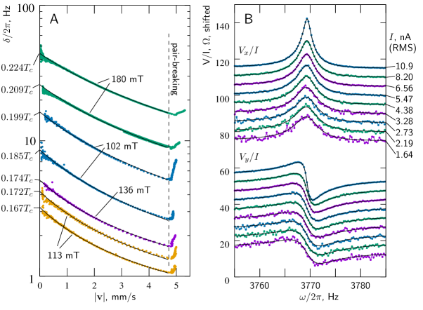
Figure 3: A: measured $\delta(|{\bf v}|)$ at seven different temperatures and magnetic fields, at zero pressure. Black lines show the fitting model with same intrinsic damping and same function $S(c)$ for all data. Temperatures (in $T_{c}$ units) are shown in assumption that $s_{0}=1$. B. Frequency sweeps at nine different drive currents are fitted together with the non-linear equation (20) using intrinsic damping and function $S(c)$ from Fig. 3A, and usual set of free parameters for Lorentzian fitting: complex amplitude, complex offset, $\omega_{0}$ and $\delta(v=0)$

On Fig. 3A. an example of measured $\delta$ at zero pressure and seven different temperatures and magnetic fields is shown as a function of velocity $|{\bf v}|$. A NbTi wire with $d=4.5\,\mu$m and $L=1.49\,$mm is used. Intrinsic width of NbTi wire partially originates from motion of vortices in the superconductor and depends on magnetic field as

$$\delta_{i}(B)=\delta^{i}_{0}+\delta^{i}_{2}B^{2}.$$ (24)

This field dependence can be obtained from measurements of the wire resonance in vacuum or by using two fitting parameters in $\delta(|{\bf v}|)$. This is done on Fig. 3A: seven datasets are fitted together using model with 7+5 parameters: temperature of each measurement, intrinsic damping $\delta^{i}_{0}$ and $\delta^{i}_{2}$, and function $S$ described via parameters $s_{0}$, $s_{1}$, $s_{2}$ introduced in (18). Because $v_{0}$ and $\delta_{0}$ have different dependence on temperature (6) by this kind of fitting it could be possible to extract temperature without external calibration. Unfortunately, temperature and $s_{0}$ have big mutial covariance and accuracy of this self-calibration for our data is poor. For obtaining good temperature calibraition it’s better to get value of $s_{0}$ from some external calibration or use theoretical value $s_{0}=1$. But regardless of this choice we will have an accurate model which can be used to extrapolate $\delta$ to $v=0$ and remove all effects of the non-linear regime. In all following figures obtaind model will be used in this way. Temperature calibration can be done as a next independent step.

On Fig. 3B an example of frequency sweeps at nine different drive currents is shown. All data are fitted together with equation (20) using intrinsic damping and function $S(c)$ obtained from Fig. 3A and usual set of free parameters for Lorentzian fitting: complex amplitude, complex offset, $\omega_{0}$ and $\delta(v=0)$. On Fig. 4A damping for same frequency sweeps is obtained by fitting them separately with either Lorentzian formula or non-linear equation (20). One can see that even at small currents Lorentzian fit gives noticeably smaller damping then the ”linear” value $\delta(v=0)$.

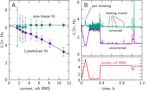
Figure 4: A: Damping parameter $\delta$ obtained by usual Lorentzian fit of frequency sweeps from Fig. 3B (lower points); $\delta(v=0)$ found by fitting same data with the non-linear formula (20) (upper points). Black horizontal line is $\delta(v=0)=6.213$ found on Fig. 3B by fitting all sweeps together. B: An example of measurement of $\delta$ as a function of time in ”tracking mode”. Current (lower plot) is ramped up and down to reach pair-breaking regime and then kept constant with a few step adjustments. Measured value of $\delta$ and corrected value $\delta(v=0)$ are shown on the upper plot. One can see that corrected value does not depend on drive current (except the pair-breaking regime) and can be used for temperature measurement. Small peaks are random heating events in helium caused by natural radioactivity.

On Fig. 4B an example of a ”tracking mode” measurement is shown. This is similar to the ”amplitude sweep” described above: damping $\delta$ is extracted from a single measurement of voltage components using (23). Normally this is the way of measuring temperature as a function of time at constant drive, but here a few changes in drive have been done: in the beginning current was ramped up and down to get information about non-linear regime and reach pair-braking velocity. Then current was increased to do measurements in the non-linear regime where signal-to-noise ratio is better. At the end current have been adjusted again. On the plot one can see measured value of $\delta$ and corrected value $\delta(v=0)$. As expected, the corrected value does not depend on drive current (except in the pair-breaking regime) and can be used for temperature measurement. Small peaks are random heating events in helium caused by natural radioactivity.

Conclusion

This note shows importance of non-linear effects for vibrating-wire thermometry in superfluid ³He-B. Method of removing the non-linearity is described and tested on experimental data. It is possible to build a simple model with a few parameters (intrinsic damping and function $S(c)$) which works at any temperature within ballistic regime (below $0.3T_{c}$) and any magnetic field.

I would like to thank A.Shen, S.Loktev, D.Zmeev and S.Autti for useful discussions.

References

- [1] S. N. Fisher, A. M. Guénault, C. J. Kennedy and G. R. Pickett “Beyond the two-fluid model: Transition from linear behavior to a velocity-independent force on a moving object in ” In Phys. Rev. Lett. 63 American Physical Society, 1989, pp. 2566–2569 DOI: 10.1103/PhysRevLett.63.2566
- [2] S. N. Fisher, G. R. Pickett and R. J. Watts-Tobin “A microscopic calculation of the force on a wire moving through superfluid3He-B in the ballistic regime” In Journal of Low Temperature Physics 83.3, 1991, pp. 225–235 URL: https://doi.org/10.1007/BF00682120
- [3] M. P. Enrico, S. N. Fisher and R. J. Watts-Tobin “Diffuse scattering model of the thermal damping of a wire moving through superfluid3He-B at very low temperatures” In Journal of Low Temperature Physics 98.1, 1995, pp. 81–89 URL: https://doi.org/10.1007/BF00754069