Discrete-time Competing-Risks Regression with or without Penalization

Abstract

Many studies employ the analysis of time-to-event data that incorporates competing risks and right censoring. Most methods and software packages are geared towards analyzing data that comes from a continuous failure time distribution. However, failure-time data may sometimes be discrete either because time is inherently discrete or due to imprecise measurement. This paper introduces a novel estimation procedure for discrete-time survival analysis with competing events. The proposed approach offers two key advantages over existing procedures: first, it expedites the estimation process for a large number of unique failure time points; second, it allows for straightforward integration and application of widely used regularized regression and screening methods. We illustrate the benefits of our proposed approach by conducting a comprehensive simulation study. Additionally, we showcase the utility of our procedure by estimating a survival model for the length of stay of patients hospitalized in the intensive care unit, considering three competing events: discharge to home, transfer to another medical facility, and in-hospital death.

Keywords  Competing events; Regularized Regression; Penalized Regression; Sure Independent Screening; Survival Analysis

1 Introduction

Most survival analysis methods and software are designed for data with continuous failure time distributions. However, there are cases where failure times are discrete, either because the time unit is discrete or due to measurement inaccuracies. For instance, in the US, the shift in presidential party control only happens every four years in January ¹. In some cases, events can happen at any point in time, but only the time interval in which each event occurred is recorded in available data. For instance, death from cancer recorded in months since diagnosis ². It is commonly recognized that using standard continuous-time models on discrete-time data without proper adjustments can lead to biased estimators for discrete-time models ^{2, 3}.

Competing events occur when individuals are susceptible to several types of events but can only experience at most one event at a time. If multiple events can happen simultaneously, they can be treated as a separate event type ⁴. For instance, competing risks in a study of hospital length of stay could be discharge and in-hospital death, where the occurrence of one of these events prevents observation of the other event for the same patient. Another classic example of competing risks is cause-specific mortality, such as death from heart disease, cancer, or other causes ⁴, ⁵.

The motivation for this project is to analyze data of length of stay (LOS) of patients in healthcare facilities. LOS typically refers to the number of days a patient stays in the hospital during a single admission ^{6, 7}. Accurate prediction of LOS is crucial for hospital management and planning of bed capacity, as it affects healthcare delivery access, quality, and efficiency ⁶. In particular, hospitalizations in intensive care units (ICU) consume a significant amount of hospital resources per patient ⁸. In this study, we use the publicly available Medical Information Mart for Intensive Care (MIMIC) - IV (version 2.0) data ⁹, ¹⁰ to develop a model for predicting LOS in ICU based on patients’ characteristics upon arrival in ICU. The study involves 25,170 ICU admissions from 2014 to 2020 with only 28 unique times, resulting in many tied events at each time point. The three competing events analyzed were: discharge to home (69.0%), transfer to another medical facility (21.4%), and in-hospital death (6.1%). Patients who left the ICU against medical advice (1.0%) were considered censored, and administrative censoring was imposed for patients hospitalized for more than 28 days (2.5%).

Regression analysis of continuous-time survival data with competing risks can be performed using standard non-competing events tools because the likelihood function for the continuous-time setting can be factored into likelihoods for each cause-specific hazard function ⁴. However, this is not the case for some regression models of discrete-time survival data with competing risks ¹. The literature on discrete-time survival data with competing risks can be categorized into two primary groups. The first group involves cause-specific hazard functions that serve as a natural and direct analogy to those found in the continuous survival time context. In this case, the cause-specific hazard function is solely dependent on the parameters of the specific competing event ^{1, 2, 3}. As this formulation results in a likelihood that cannot be decomposed into distinct components for each type of event, Allison ¹ explored an alternative, more manageable formulation. In particular, he introduced a cause-specific hazard function that depends not only on the parameters associated with the specific competing event but also on the parameters related to all other event types. This cause-specific hazard formulation was later adopted and further developed by others ^{11, 12, 13}. As noted by Allison ¹, the advantage of the second approach is a significant simplification of the estimation procedure, albeit at the cost of interpretability. For additional technical details comparing these two approaches, please refer to Section 5 below. We choose to align with Lee et al. ² and work with the natural and direct analogy to the cause-specific hazard function in the context of continuous survival time, as this formulation of cause-specific hazard models provides a simpler interpretation.

Lee et al. ² showed that if one naively treats competing events as censoring in the discrete-time likelihood, separate estimation of cause-specific hazard models for different event types may be accomplished using a collapsed likelihood which is equivalent to fitting a generalized linear model to repeated binary outcomes. Moreover, the maximum collapsed-likelihood estimators are consistent and asymptotically normal under standard regularity conditions, which gives rise to Wald confidence intervals and likelihood-ratio tests for the effects of covariates. Wu et al. ³ focused on two competing events and used a different approach than that of Lee et al. ². However, they noted that it leads to the same estimators. The contribution of Wu et al. ³ is mainly by allowing an additional fixed effect of medical center in the model.

In this work we provide a new estimation procedure for analysing discrete survival time data with competing events. We simplify and speed up the estimation process based on the collapsed-likelihood approach of Lee et al. ². Our approach allows for the use of common penalized regression methods like lasso and elastic net among others ¹⁴ and enables easy implementation of screening methods for high-dimensional data, such as sure independent screening ^{15, 16, 17, 18}. Our Python software, PyDTS ¹⁹, implements both our method and the one from Lee et al. ² and other tools for discrete-time survival analysis.

The rest of the article is structured as follows. Section 2 summarizes the collapsed likelihood of Lee et al.² and thoroughly explains the proposed estimation approach. Section 3 presents the results of a comprehensive simulation study, demonstrating the superiority of our method in terms of computational efficiency and showcasing the utilization of regularized regression and screening methods. Section 4 demonstrates the use of our method on the ICU LOS data of MIMIC. Finally, Section 5 concludes with a short discussion.

2 Methods

2.1 Notation and Models

Let $T$ be a discrete event time that can take on only the values ${1,2,\ldots,d}$, and let $J$ represent the type of event, with $J\in\{1,\ldots,M\}$. Also, consider a $p\times 1$ vector of time-independent covariates $Z$. The setting of time-dependent covariates will be discussed later. A general discrete cause-specific hazard function is of the form

$$\lambda_{j}(t|Z)=\Pr(T=t,J=j|T\geq t,Z)\hskip 2.84544pt,\hskip 8.5359ptt=1,2,\ldots,d\hskip 2.84544pt,\hskip 8.5359ptj=1,\ldots,M\,.$$

As described by Allison ¹, the semi-parametric models for the hazard functions, based on a regression transformation model, can be represented as

$$h(\lambda_{j}(t|Z))=\alpha_{jt}+Z^{T}\beta_{j}\hskip 2.84544pt,\hskip 8.5359ptt=1,2,\ldots,d\hskip 2.84544pt,\hskip 8.5359ptj=1,\ldots,M\,,$$

where $h$ is a known function. The total number of unknown parameters is $M(d+p)$. Having a shared $Z$ among the $M$ models does not necessitate the use of identical covariates in all the models. Because the regression coefficients $\beta_{j}$ are specific to each event type, any coefficient can be zeroed out to exclude its associated covariate. We adopt the popular logit function $h(a)=\log\{a/(1-a)\}$ and get

$$\lambda_{j}(t|Z)=\frac{\exp(\alpha_{jt}+Z^{T}\beta_{j})}{1+\exp(\alpha_{jt}+Z^{T}\beta_{j})}\,.$$ (1)

Leaving $\alpha_{jt}$ unspecified is similar to an unspecified baseline hazard function in the Cox proportional hazard model ²⁰. Thus, the model described above is considered a semi-parametric model in discrete time.

Let $S(t|Z)=\Pr(T>t|Z)$ be the overall survival given $Z$. Then, the probability of experiencing event of type $j$ at time $t$, $t=1,\ldots,d$, $j=1,\ldots,M$, equals

$$\Pr(T=t,J=j|Z)=\lambda_{j}(t|Z)S(t-1|Z)=\lambda_{j}(t|Z)\prod_{k=1}^{t-1}\left\{1-\sum_{j^{\prime}=1}^{M}\lambda_{j^{\prime}}(k|Z)\right\}$$

and the probability of event type $j$ by time $t$ given $Z$, also known as the cumulative incident function (CIF) of cause $j$ is given by

$$F_{j}(t|Z)=\sum_{k=1}^{t}\lambda_{j}(k|Z)\prod_{l=1}^{k-1}\left\{1-\sum_{j^{\prime}=1}^{M}\lambda_{j^{\prime}}(l|Z)\right\}\,.$$

Finally, the marginal probability of event type $j$, given $Z$, equals

$$\Pr(J=j|Z)=\sum_{t=1}^{d}\lambda_{j}(t|Z)\prod_{k=1}^{t-1}\left\{1-\sum_{j^{\prime}=1}^{M}\lambda_{j^{\prime}}(k|Z)\right\}\,.$$

Our goal is estimating the parameters

$$\Omega=(\alpha_{11},\ldots,\alpha_{1d},\beta_{1}^{T},\ldots,\alpha_{M1},\ldots,\alpha_{Md},\beta_{M}^{T})\,.$$

2.2 The Collapsed Log-Likelihood Approach of Lee et al.

For clarity, the estimation method of Lee et al. ² that employs a collapsed log-likelihood approach is briefly summarized. For simplicity, we temporarily assume two competing events, i.e., $M=2$, with the aim of estimating $\Omega=(\alpha_{11},\ldots,\alpha_{1d},\beta_{1}^{T},\alpha_{21},\ldots,\alpha_{2d},\beta_{2}^{T})$. The data consist of $n$ independent observations, each with $(X_{i},\delta_{i},J_{i},Z_{i})$ where $X_{i}=\min(C_{i},T_{i})$, $C_{i}$ is a discrete right-censoring time, $\delta_{i}=I(T_{i}\leq C_{i})$ is the event indicator and $J_{i}\in\{0,1,2\}$, where $J_{i}=0$ if and only if $\delta_{i}=0$, $i=1,\ldots,n$. It is assumed that given the covariates, the censoring and failure times are independent and non-informative in the sense of Kalbfleisch and Prentice ⁴ (Section 3.2). Then, the likelihood function is proportional to

$$L = \prod_{i=1}^{n}\left\{\frac{\lambda_{1}(X_{i}|Z_{i})}{1-\lambda_{1}(X_{i}|Z_{i})-\lambda_{2}(X_{i}|Z_{i})}\right\}^{I(J_{i}=1)}\left\{\frac{\lambda_{2}(X_{i}|Z_{i})}{1-\lambda_{1}(X_{i}|Z_{i})-\lambda_{2}(X_{i}|Z_{i})}\right\}^{I(J_{i}=2)}\prod_{t=1}^{X_{i}}\{1-\lambda_{1}(t|Z_{i})-\lambda_{2}(t|Z_{i})\}\,.$$

Equivalently,

$$L = \prod_{i=1}^{n}\left[\prod_{j=1}^{2}\prod_{t=1}^{X_{i}}\left\{\frac{\lambda_{j}(t|Z_{i})}{1-\lambda_{1}(t|Z_{i})-\lambda_{2}(t|Z_{i})}\right\}^{\delta_{jit}}\right]\prod_{t=1}^{X_{i}}\{1-\lambda_{1}(t|Z_{i})-\lambda_{2}(t|Z_{i})\}$$

and the log-likelihood (up to a constant) becomes

$$\log L = \sum_{i=1}^{n}\left[\sum_{j=1}^{2}\sum_{t=1}^{X_{i}}\left[\delta_{jit}\log\lambda_{j}(t|Z_{i})-\delta_{jit}\{1-\lambda_{1}(t|Z_{i})-\lambda_{2}(t|Z_{i})\}\right]+\sum_{t=1}^{X_{i}}\log\{1-\lambda_{1}(t|Z_{i})-\lambda_{2}(t|Z_{i})\}\right]$$

$$= \sum_{i=1}^{n}\sum_{t=1}^{X_{i}}\left[\delta_{1it}\log\lambda_{1}(t|Z_{i})+\delta_{2it}\log\lambda_{2}(t|Z_{i})+\{1-\delta_{1it}-\delta_{2it}\}\log\{1-\lambda_{1}(t|Z_{i})-\lambda_{2}(t|Z_{i})\}\right]\,,$$

where $\delta_{jit}$ equals one if subject $i$ experienced event of type $j$ at time $t$; and 0 otherwise. Evidently, in contrast to the continuous-time setting with competing events, $L$ cannot be decomposed into separate likelihoods for each cause-specific hazard function $\lambda_{j}$. Estimating the vector of parameters $\Omega$ through maximizing $\log L$ would entail maximizing with respect to $M(d+p)$ parameters simultaneously, leading to a time-consuming process.

Alternatively, Lee et al.² suggested the following collapsed log-likelihood approach. The dataset is expanded such that for each observation $i$ the expanded dataset includes $X_{i}$ rows, i.e., dummy observations, one row for each time $t$, $t\leq X_{i}$; see Table 1. Specifically, for each row $t$, $t\leq X_{i}$, $\tilde{X_{i}}=t$, and the following two binary indicators are defined $\delta_{jit}=I(T_{i}=t,J_{i}=j)$, $j=1,2$. At each time point $t$, the dummy observations can be considered as random variables from a conditional multinomial distribution with one of three possible outcomes $\{\delta_{1it},\delta_{2it},1-\delta_{1it}-\delta_{2it}\}$. Then, estimation of $(\alpha_{11},\ldots,\alpha_{1d},\beta_{1}^{T})$ is based on a collapsed log-likelihood such that $\delta_{2it}$ and $1-\delta_{1it}-\delta_{2it}$ are combined. The collapsed log-likelihood for cause $j=1$ based on a binary regression model with $\delta_{1it}$ as the outcome is given by

$$\log L_{1}=\sum_{i=1}^{n}\sum_{t=1}^{X_{i}}\left[\delta_{1it}\log\lambda_{1}(t|Z_{i})+(1-\delta_{1it})\log\{1-\lambda_{1}(t|Z_{i})\}\right]\,.$$

Similarly, the collapsed log-likelihood for cause $j=2$ with $\delta_{2it}$ as the outcome becomes

$$\log L_{2}=\sum_{i=1}^{n}\sum_{t=1}^{X_{i}}\left[\delta_{2it}\log\lambda_{2}(t|Z_{i})+(1-\delta_{2it})\log\{1-\lambda_{2}(t|Z_{i})\}\right]\,,$$

and one can fit the two models, separately.

In general, for $M$ competing events, the estimators of $(\alpha_{j1},\ldots,\alpha_{jd},\beta_{j}^{T})$, $j=1,\ldots,M$, are the respective values that maximize

$$\log L_{j}=\sum_{i=1}^{n}\sum_{t=1}^{X_{i}}\left[\delta_{jit}\log\lambda_{j}(t|Z_{i})+(1-\delta_{jit})\log\{1-\lambda_{j}(t|Z_{i})\}\right]\quad j=1,\ldots,M\,.$$ (2)

Namely, each maximization $j$ consists of $d+p$ parameters. Lee et al. showed that the estimators are asymptotically multivariate normally distributed and the covariance matrix can be consistently estimated. As the likelihood $L$ does not decompose into distinct components for the various event types, maximizing the collapsed likelihood functions $L_{j}$ independently for each event type does not yield equivalent estimates compared to maximizing the full likelihood function concurrently over the model parameters for all event types. There is a trade-off between computational simplicity and potential loss of efficiency.

2.3 The Proposed Approach

We use the collapsed log-likelihood approach and simplify the estimation process further. The proposed method offers two improvements over Lee et al.²: (1) substantial reduction in computation time for high values of $d$ and large sample sizes; (2) easy integration of penalized regression techniques (ridge, lasso, elastic net, among others) and screening methods.

Lee et al.² suggested the collapsed log likelihoods and noted that for each $\log L_{j}$ standard generalized linear models (GLM) can be used. They also commented that because of the Markov property, for example, conditional independence of the binary variables, the naive variance estimator from GLM of each event type, which assumes independence, is valid. We adopt the expanded data suggested by Lee et al. (2018). However, instead of using their collapsed log-likelihood directly, we use the conditional logistic regression approach  ^{21, 22} in order to separate between the estimation procedure of $\alpha_{jt}$, $t=1,\ldots,d$ and $\beta_{j}$ within each event type $j$, $j=1,\ldots,M$. In particular, a likelihood based on conditional logistic regression is replacing Eq. (2), while stratifying the expanded dataset according to $\tilde{X}$ and conditioning on the number of events within each stratum, $\sum_{i\in\mathcal{N}_{t}}\delta_{jit}$, were $\mathcal{N}_{t}$ as the set of all dummy observations with $\tilde{X}$ equal to $t$ , and thus $\alpha_{jt}$ are eliminated.

Specifically, define $d_{jt}$ as a vector of 0s and 1s with a length equal to the cardinality of the set $\mathcal{N}_{t}$, where $d_{jit}$ represents its components. Also, let $S_{jt}$ be the set of all possible vectors $d_{jt}$ such that $\sum_{i\in\mathcal{N}_{t}}d_{jit}=\sum_{i\in\mathcal{N}_{t}}\delta_{jit}$. Then, the conditional likelihoods of the expanded data, while stratifying by $\tilde{X}$ and given $\sum_{i\in\mathcal{N}_{t}}\delta_{jit}$, $t=1,\ldots,d$, are given by

$$L_{j}^{\mathcal{C}}(\beta_{j})=\prod_{t=1}^{d}\frac{\exp(\sum_{i\in\mathcal{N}_{t}}\delta_{jit}Z_{i}^{T}\beta_{j})}{\sum_{d_{jt}\in\mathcal{S}_{jt}}\exp(\sum_{i\in\mathcal{N}_{t}}d_{jit}Z_{i}^{T}\beta_{j})}\,\,\,,\,\,\,j=1,\ldots,M\,.$$ (3)

Since Eq. (3) has a form of partial likelihood of a Cox regression model when ties are present (see, for example, Eq. (8.4.3) of ⁵), an available Cox-model routine can be used for estimating $\beta_{j}$, $j=1,\ldots,M$. The clogit function of R uses this trick and estimates a logistic regression model by maximizing the conditional likelihood. It creates the necessary dummy variable of times and the strata, then calls coxph. The clogit function uses the Breslow approximation for the conditional likelihood as a default, but the exact form and other common approximations for ties are also available. Clearly, the use of available Cox model routine for maximizing Eq. (3) is only a mathematical trick while Eq. (1) still holds.

As we are segregating the estimation procedure for $\beta_{j}$ and $\alpha_{jt}$, by the use of conditional likelihood, estimating equations for $\alpha_{jt}$ are required. Using the estimators of $\beta_{j}$, $\widehat{\beta}_{j}$, $j=1,\ldots,M$, we propose estimating $\alpha_{jt}$, $j=1,\ldots,M$, $t=1,\ldots,d$, through a series of $Md$ single-dimensional optimization algorithms applied to the original (i.e., non-expanded) dataset such that

$$\widehat{\alpha}_{jt}=\mbox{argmin}_{a}\left\{\frac{1}{Y.(t)}\sum_{i=1}^{n}I(X_{i}\geq t)\frac{\exp(a+Z_{i}^{T}\widehat{\beta}_{j})}{1+\exp(a+Z_{i}^{T}\widehat{\beta}_{j})}-\frac{N_{j}(t)}{Y.(t)}\right\}^{2}\,\,\,,\,\,\,j=1,\ldots,M\,,\,\,\,t=1,\ldots,d\,\,\,,$$ (4)

where $Y.(t)=\sum_{i=1}^{n}I(X_{i}\geq t)$ and $N_{j}(t)=\sum_{i=1}^{n}I(X_{i}=t,J_{i}=j)$. Eq. (4) involves minimizing the squared difference between the observed proportion of failures of type $j$ at time $t$, i.e., $N_{j}(t)/Y.(t)$, and the expected proportion of failures, as determined by Model (1) and $\widehat{\beta}_{j}$.

In summary, the proposed estimation procedure consists of the following two speedy steps:

1. Using the expanded dataset, estimate each vector $\beta_{j}$ individually, $j=1,\ldots,M$, by maximizing Eq. (3) using a stratified Cox routine, such as the clogit function in the survival R package.

2. Using $\widehat{\beta}_{j}$ , $j=1,\ldots,M$, of Step 1 and the original non-expanded dataset, estimate each $\alpha_{jt}$, $j=1,\ldots,M$, $t=1,\ldots,d$, separately, by Eq. (4).

The simulation results in Section 3 show that the above two-step procedure performs well in terms of bias and provides similar standard errors to those of Lee et al. However, for large values of $d$, the two-step procedure leads to a substantial gain in computation time compared to estimating $p+d$ parameters simultaneously. Estimating $d$ single-dimensional parameters and one $p$-dimensional parameter is often faster than estimating $p+d$ parameters together.

The advancement in data collection technologies has resulted in a significant increase in the number of potential predictors. Separating the estimation of $\beta_{j}$ and $\alpha_{jt}$ is highly relevant in dimension reduction or model selection regression problems, as, for instance, applying methods that keep a subset of predictors and discard the rest would only involve working with $\beta_{j}$. Here are two examples:

1. Regularized regression ¹⁴. Penalized regression methods (e.g., lasso, adaptive lasso, elastic net) place a constraint on the size of the regression coefficients. We propose to apply penalized regression methods in Lagrangian form based on Eq. (3) by minimizing

   $$-\log L_{j}^{\mathcal{C}}(\beta_{j})+\eta_{j}P(\beta_{j})\,\,\,,\,\,\,j=1,\ldots,M\,,$$ (5)

   where $P$ is a penalty function and $\eta_{j}>0$ is a shrinkage tuning parameter. For instance, in the $l_{1}$ penalty employed by lasso, $P(\beta_{j})=\sum_{k=1}^{p}|\beta_{jk}|$. In the case of $l_{2}$ regularization for ridge regression, $P(\beta_{j})=\sum_{k=1}^{p}\beta^{2}_{jk}$. Elastic net, on the other hand, involves an additional set of tuning parameters to balance between lasso and ridge regression (see ¹⁴ for additional penalty functions). Clearly, any routine of regularized Cox regression model can be used for estimating $\beta_{j}$, $j=1,\ldots,M$, based on Eq. (5) (e.g., glmnet of R or CoxPHFitter of Python). Finally, the parameters $\alpha_{jt}$ are estimated only once the regularization step is completed and models are selected.

2. Sure independent screening. Under ultra-high dimension settings, most of the regularized methods suffer from the curse of dimensionality, high variance and over-fitting^{14, 23}. To overcome these issues, the marginal screening technique, sure independent screening (SIS) has been shown to filter out many uninformative variables under an ordinary linear model with normal errors ¹⁵. Subsequently, penalized variable selection methods are often applied to the remaining variables. The key idea of the SIS procedure is to rank all predictors by using a utility measure between the response and each predictor and then to retain the top variables. The SIS procedure has been extended to various models and data types such as generalized linear models ²⁴, additive models ²⁵, and Cox regression models ^{16, 17, 18}. We propose to adopt the vanilla screening method based on Eq. (3); for more details see Appendix E.

The consistency and asymptotic normality of each $\widehat{\beta}_{j}$, $j=1,\ldots,M$, follow a similar argument of Lee et al. (2018). Namely, due to the Markov property, which includes conditional independence of the binary variables, the properties of estimators from the conditional logistic regression approach above which assumes independence remain valid, as $n\rightarrow\infty$ and under finite fixed values of $d$ and $M$. The consistency and asymptotic normality of each $\widehat{\alpha}_{jt}$, $j=1,\ldots,M$, $t=1,\ldots,d$, are derived in Appendix A.

The above proposed estimation procedure can easily handle covariates or coefficients that change over time, $Z(t)$ and $\beta_{j}(t)$, respectively. Similarly to the Cox model with continuous survival time, the simplest way to code time-dependent covariates uses intervals of time. Then, the data is encoded by breaking the individual’s time into multiple time intervals, with one row of data for each interval. Hence combining this data expansion step with the expansion described in Table 1 is straightforward. For time-dependent coefficients, $\beta_{j}(t)$, Eq. (3) is replaced by

$$L_{j}^{\mathcal{C}}(\beta_{j}(t))=\frac{\exp\{\sum_{i\in\mathcal{N}_{t}}\delta_{jit}Z_{i}^{T}\beta_{j}(t)\}}{\sum_{d_{jt}\in\mathcal{S}_{t}}\exp\{\sum_{i\in\mathcal{N}_{t}}d_{jit}Z_{i}^{T}\beta_{j}(t)\}}\,\,\,,\,\,\,j=1,\ldots,M\,,\,t=1,\ldots,d\,.$$

Clearly, one can easily combine time-dependent covariate with time-dependent coefficients.

3 Simulation Study

We evaluated and demonstrated the utility of our proposed approach through a comprehensive simulation study, comparing it with Lee et al. ². The simulation study aimed to assess performance, compare timing, and showcase the integration of regularization (e.g., lasso) and screening methods (e.g., SIS and SIS-L) into the two-step procedure, including estimating the tuning parameters. The simulation settings are summarized in Table 2.

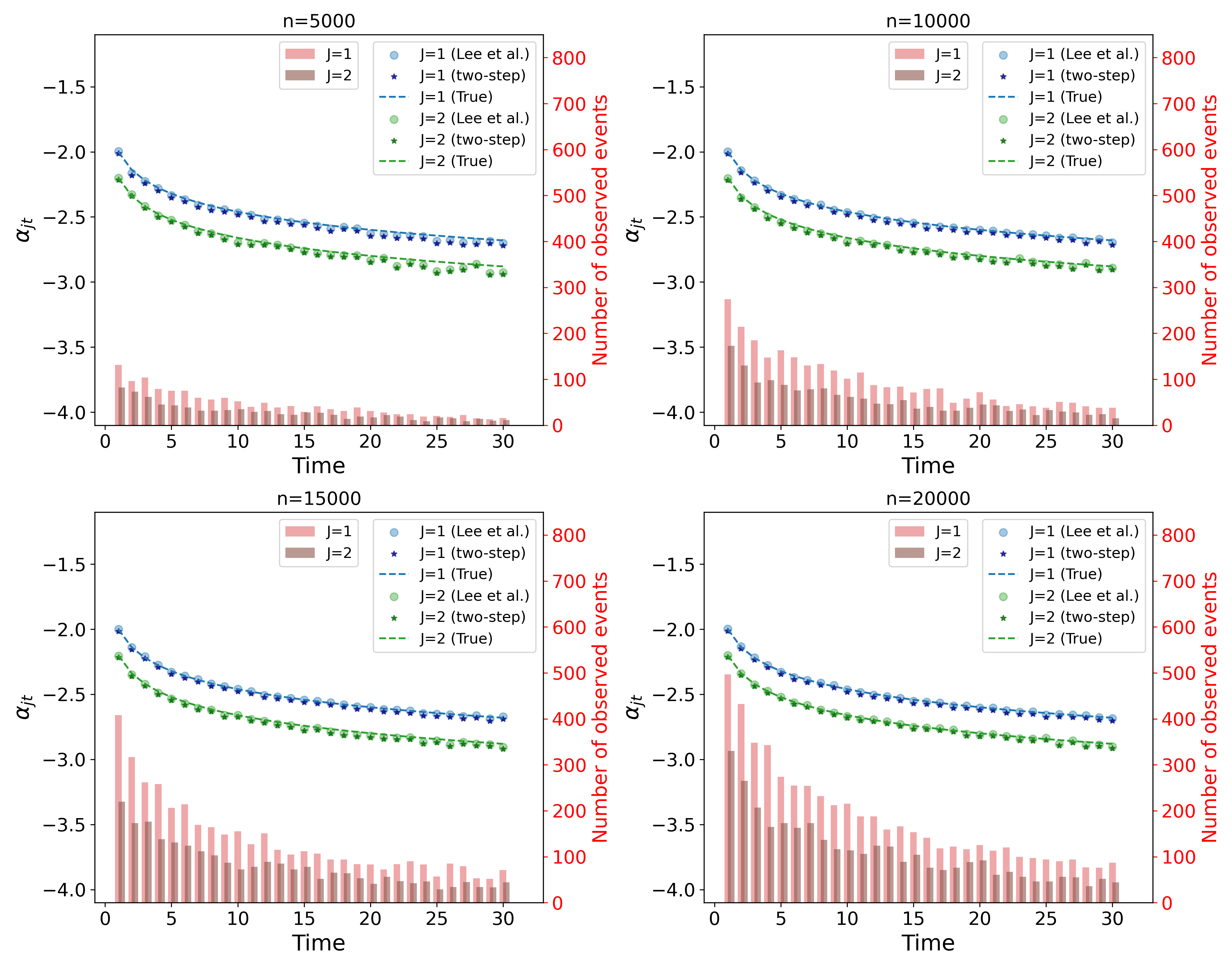
Figure 1: Simulation results of two competing events. Results of ${\alpha}_{jt}$. Each panel is based on a different sample size. Number of observed events are shown in red and brown bars for event types $j=1$ and $j=2$, respectively. True values and mean of estimates are in blue and green for $j=1$ and $j=2$. True values are shown in dashed lines, mean of estimates based on Lee et al. and the proposed two-step approach denoted by circles and diamonds, respectively.

The sampling procedure begins with the selection of covariates $Z$, a vector of $p$ dimension, for each individual. Subsequently, the type of event is sampled based on the probabilities $\Pr(J=j|Z)$, and finally the event time is sampled based on $\Pr(T=t|J=j,Z)=\Pr(T=t,J=j|Z)/\Pr(J=j|Z)$. For simulation settings 1-16, each covariate was sampled from a standard uniform distribution. The parameters’ values of Settings 1-8 were set to be $\alpha_{1t}=-2.0-0.2\log t$, $\alpha_{2t}=-2.2-0.2\log t$, $t=1,\ldots,30$, $\beta_{1}=-(\log 0.8,\log 3,\log 3,\log 2.5,\log 2)^{T}$, and $\beta_{2}=-(\log 1,\log 3,\log 4,\log 3,\log 2)^{T}$. Finally, the censoring times were sampled from a discrete uniform distribution with probability 0.01 at each $t$. Table 3 and Fig. 1 summarise the results of $\beta_{j}$ and $\alpha_{jt}$, respectively, for two competing risks, in terms of mean and standard errors. The respective results with three competing risks are provided in Appendix C, Tables S1 - S2 and Figure S1. The results of small sample sizes are provided in Appendix D Table S3 and Figure S2. Evidently, both methods perform similarly in terms of bias and standard errors. In addition, the empirical coverage rates of 95% Wald-type confidence intervals for each regression coefficient, based on the proposed approach, are reasonably close to 95%.

For demonstrating the reduction in computation time as a function of $d$ (Settings 11–16), a sample size of $n=20,000$ observations was considered with $p=10$ covariates, two competing events, various values of $d$, and 10 repetitions for each $d$. Furthermore, $\alpha_{1t}=-2.5-0.3\log t$, $\alpha_{2t}=-2.8-0.3\log t$,

$$\beta_{1}=-0.5(\log 0.8,\log 3,\log 3,\log 2.5,\log 4,\log 1,\log 3,\log 2,\log 2,\log 3)^{T}\,,$$

and

$$\beta_{2}=-0.5(\log 1,\log 3,\log 2,\log 1,\log 4,\log 3,\log 4,\log 3,\log 3,\log 2)^{T}\,.$$

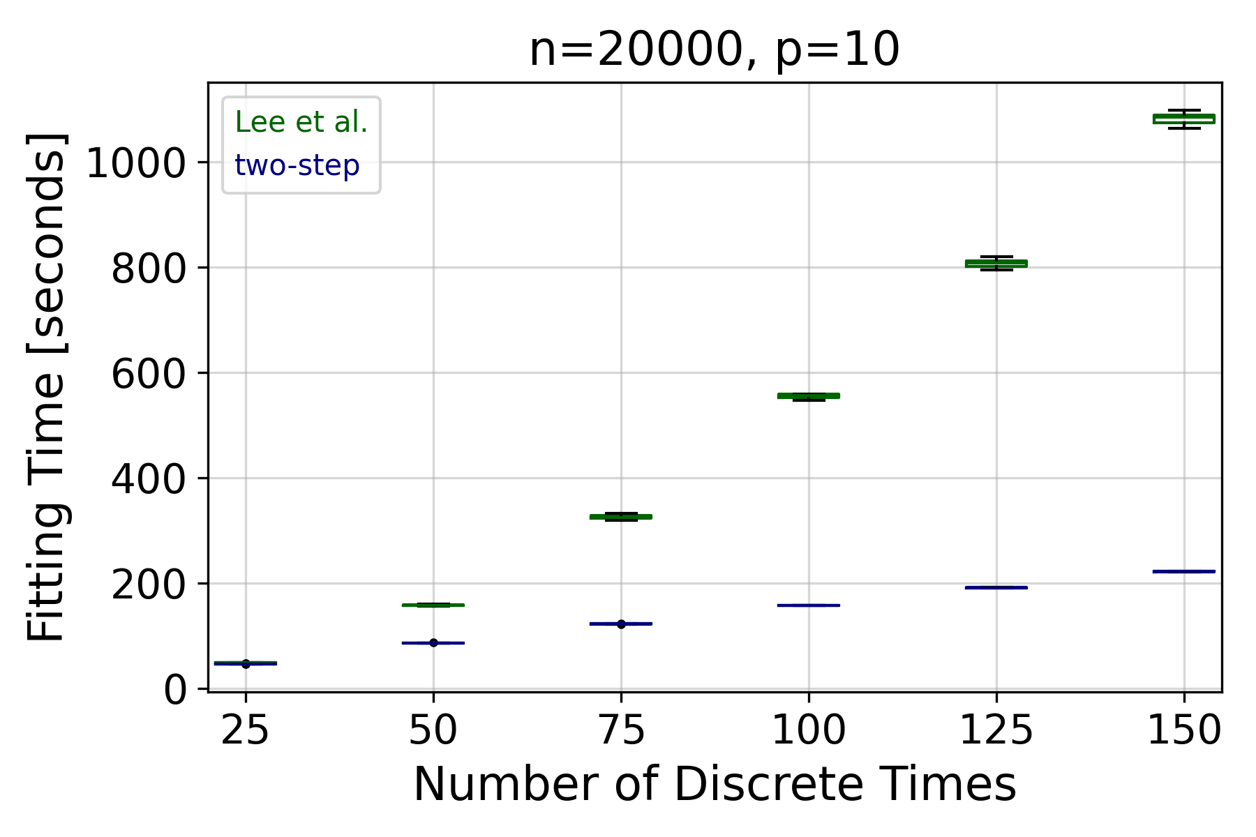
Figure 2: Simulation results: a computation time comparison between the method of Lee et al. and the proposed two-step approach.

The median and the interquartile range of the computation times are presented in Figure 2. These results are based on a single CPU out of 40 CPUs server of type Intel Xeon Silver 4114 CPU @ 2.20GHz X 2 and 377GB RAM. Evidently, under low values of $d$, the computation times of the two approaches are comparable. However, as $d$ increases, the advantage of the proposed approach, in terms of computation time, increases as well. Moreover, when running this analysis using hardware with 16GB RAM, the estimation procedure of Lee et al. reached a memory error at a low value of $d$, while the two-step procedure was completed successfully.

Finally, we provide simulation results of the proposed two-step approach with lasso regularization and sure independence screening procedures. The goal of Settings 17–18 is to demonstrate the incorporation of lasso regularization into the proposed two-step procedure for feature selection. Therefore, in these settings $p=100$ covariates were considered, but only five of them are with non-zero values. Two settings of zero-mean normally distributed covariates were considered: (i) independent covariates, each with variance 0.4; (ii) the following covariances were updated in setting (i) $Cov(Z_{1},Z_{9})=0.1$, $Cov(Z_{2},Z_{10})=0.3$, $Cov(Z_{4},Z_{8})=-0.3$, and $Cov(Z_{5},Z_{12})=-0.1$. In order to get appropriate survival probabilities based on Eq. (1), covariates were truncated to be within $[-1.5,1.5]$. The parameters of the model were set to be $\alpha_{1t}=-3.4-0.1\log t$, $\alpha_{2t}=-3.4-0.2\log t$, $t=1,\ldots,15$. The first five components of $\beta_{1}$ and $\beta_{2}$ were set to be $(1.2,1.5,-1,-0.3,-1.2)$ and $(-1.2,1,1,-1,1.4)$, respectively, and the rest of the coefficients were set to zero.

The tuning parameters $\eta_{j}$, $j=1,\ldots,M$, control the amount of regularization, hence their values play a crucial role. In this work (and in our Python package PyDTS) the values of $\eta_{j}$ are selected by K-fold cross validation while the criterion is to maximize the out-of-sample global area under the receiver operating characteristics curve (AUC). Appendix B provides the definitions and estimators of the area under the receiver operating characteristics curve and Brier score for discrete-survival data with competing risks and right censoring. This includes the cause-specific AUC and Brier score at each time $t$, $\mbox{AUC}_{j}(t)$ and $\mbox{BS}_{j}(t)$, respectively; integrated cause-specific AUC and Brier score, $\mbox{AUC}_{j}$ and $\mbox{BS}_{j}$; and global AUC and Brier score, AUC and BS.

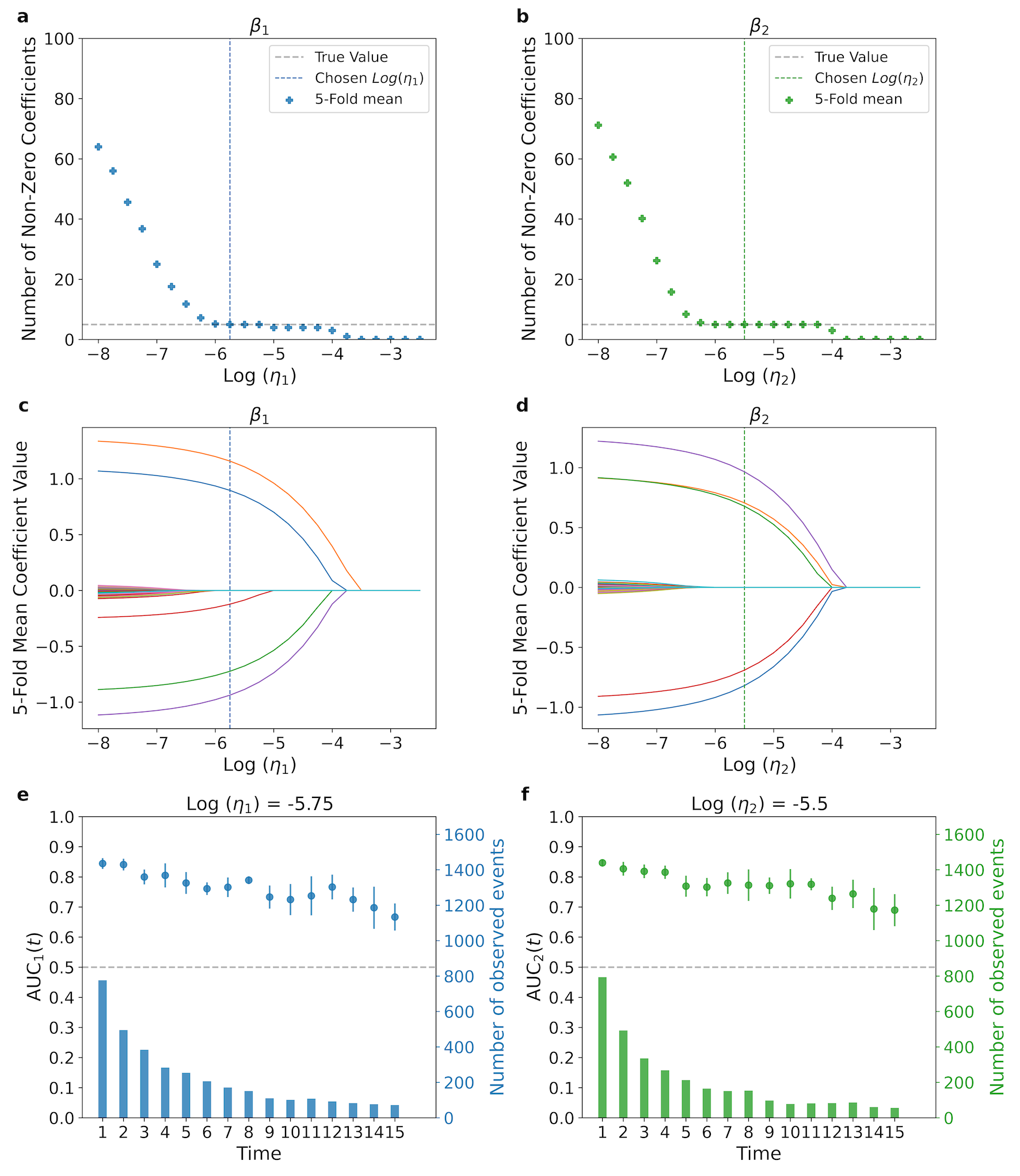
Figure 3: lasso regularization results of one simulated random sample under setting No. 17 with independent covariates (refer to Table 1 of the main text), and five out of 100 coefficients having non-zero values. Tuning parameters were selected through 5-fold cross-validation, varying $\log\eta_{j}$ from -8 to -2.5 with a step size of 0.25 (on a $\log$ for presentation ease). The chosen $\log\eta_{j}$, $j=1,2$, values, denoted by vertical dashed lines on panels a-d, resulted in five non-zero regression coefficients for each $j$. Panels a-b display the number of non-zero coefficients for events 1 and 2, respectively, with the true value (five) shown as a horizontal dashed line. Evidently, with the chosen values of $\log\eta_{j}$, the analysis resulted in five non-zero regression coefficients for each $j$. The estimates of $\beta_{j}$ as a function of $\log\eta_{j}$ are depicted in panels c and d. Each curve corresponds to a variable, and at the chosen $\log\eta_{j}$ values, each $\beta_{j}$ is reasonably close to its true value. Panels e-f show the mean (and SD bars) of the 5-fold $\widehat{\mbox{AUC}}_{1}(t)$ and $\widehat{\mbox{AUC}}_{2}(t)$, respectively, under the selected $\log\eta_{j}$ values, along with the number of observed events of event type $j$ in bars.

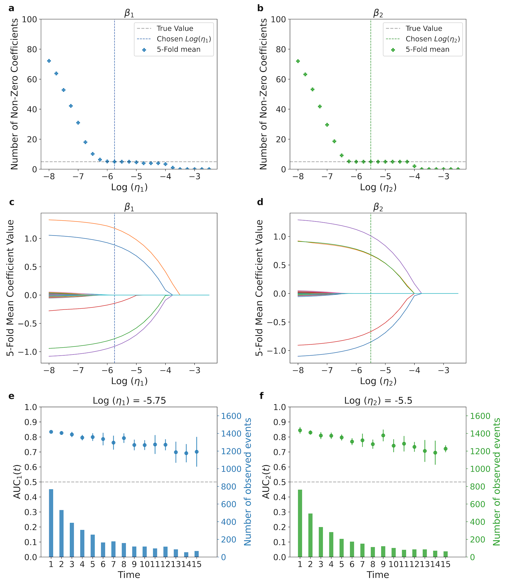
Figure 4: lasso regularization results of one simulated random sample under setting No. 18 with dependent covariates (refer to Table 1 of the main text), and five out of 100 coefficients having non-zero values. Tuning parameters were selected through 5-fold cross-validation, varying $\log\eta_{j}$ from -8 to -2.5 with a step size of 0.25 (on a $\log$ for presentation ease). The chosen $\log\eta_{j}$, $j=1,2$, values, denoted by vertical dashed lines on panels a-d, resulted in five non-zero regression coefficients for each $j$. Panels a-b display the number of non-zero coefficients for events 1 and 2, respectively, with the true value (five) shown as a horizontal dashed line. Evidently, with the chosen values of $\log\eta_{j}$, the analysis resulted in five non-zero regression coefficients for each $j$. The estimates of $\beta_{j}$ as a function of $\log\eta_{j}$ are depicted in panels c and d. Each curve corresponds to a variable, and at the chosen $\log\eta_{j}$ values, each $\beta_{j}$ is reasonably close to its true value. Panels e-f show the mean (and SD bars) of the 5-fold $\widehat{\mbox{AUC}}_{1}(t)$ and $\widehat{\mbox{AUC}}_{2}(t)$, respectively, under the selected $\log\eta_{j}$ values, along with the number of observed events of event type $j$ in bars.

Fig. 3 demonstrates the results of the regularization parameters $\eta_{j}$, $j=1,2$, of one simulated dataset under Setting 17. As expected, as the amount of regularization increases (higher values of $\eta_{j}$, $j=1,2$), the estimated coefficients of $\beta_{j}$ reduces (panels c-d), and a higher number of coefficients are set to zero (panels a-b). The selected values $\log\eta_{1}=-5.75$ and $\log\eta_{2}=-5.5$ are shown by vertical dashed lines on panels a-d. Panels a-b show the mean number of non-zero coefficients for events 1 and 2, respectively, and the true value 5 is shown in horizontal dashed line. The values of the estimated $\beta_{j}$ as a function of $\eta_{j}$ are shown in panels c and d. Panels e-f show the mean (and SD bars) of the 5-fold $\widehat{\mbox{AUC}}_{1}(t)$ and $\widehat{\mbox{AUC}}_{2}(t)$, respectively, under the selected $\log\eta_{j}$ values, along with the number of observed events of event type $j$ in bars. Similar results are shown in Figure 4 for one simulated random sample under setting 18 with dependent covariates.

Based on the one simulated dataset of Setting 17 (depicted in Fig.  3) and the selected values of $\eta_{j}$ the means and standard deviations (SD) of the 5-fold integrated cause-specific $\widehat{\mbox{AUC}}_{j}$ were $\widehat{\mbox{AUC}}_{1}=0.796$ (SD=0.007) and $\widehat{\mbox{AUC}}_{2}=0.803$ (SD=0.007), with a mean global $\widehat{\mbox{AUC}}=0.8$ (SD=0.003). The mean global AUC of the non-regularized procedure was $\widetilde{\mbox{AUC}}=0.795$ (SD=0.002). Looking at this specific example, we observe a substantial reduction in the number of covariates selected by the lasso penalty, without a significant change in the discrimination performance as measured by the AUC. The mean integrated cause-specific Brier Scores were $\widehat{\mbox{BS}}_{1}=0.045$ (SD=0.002) and $\widehat{\mbox{BS}}_{2}=0.044$ (SD=0.003), with a mean global Brier Score $\widehat{\mbox{BS}}=0.044$ (SD=0.002). Similar results were observed for the one simulated dataset of Setting 18 (depicted in Fig. 4): $\widehat{\mbox{AUC}}_{1}=0.796$ (SD=0.007), $\widehat{\mbox{AUC}}_{2}=0.801$ (SD=0.008), $\widehat{\mbox{AUC}}=0.799$ (SD=0.005), and $\widetilde{\mbox{AUC}}=0.794$ (SD=0.005). The mean Brier Scores were $\widehat{\mbox{BS}}_{1}=0.046$ (SD=0.002), $\widehat{\mbox{BS}}_{2}=0.043$ (SD=0.003), and $\widehat{\mbox{BS}}=0.045$ (SD=0.001). The results of Setting 19 reveal that the mean of true- and false-positive discoveries for each event type, $\mbox{TP}_{j}$ and $\mbox{FP}_{j}$, $j=1,2$, under the selected values of $\eta_{j}$ were $\mbox{TP}_{1}=4.99$, $\mbox{FP}_{1}=0.01$, $\mbox{TP}_{2}=5$, and $\mbox{FP}_{2}=0$. The results indicate that the correct model was selected in all the 100 repetitions, except for a single run for $j=1$. Appendix E provides a detailed description of Settings 20–22, where we demonstrate the integration of screening methods into the two-step procedure, and its results.

4 MIMIC Data Analysis - Length of Hospital Stay in ICU

Although the MIMIC dataset records admission and discharge times in minute-level resolution, it is advisable to conduct survival analysis in discrete units of days. This is because the times of admission and discharge within a day are heavily influenced by hospital staff and regulations, and are less indicative of the patients’ health status. The present study examines 25,170 ICU admissions (48.8% female) between 2014 and 2020, with a total of 28 unique days. The study considers three competing events: discharge to home ($J=1$, 69.0%), transfer to another medical facility ($J=2$, 21.4%), and in-hospital death ($J=3$, 6.1%). Patients who left the ICU against medical advice (1.0%) were treated as censored data, and administrative censoring was applied for patients who were hospitalized for more than 28 days (2.5%).

The following analysis is restricted to admissions classified as “emergency”, with a distinction between direct emergency and emergency ward (EW). In case of multiple admissions per patient, the latest one is included. Emergency admission history is included by two covariates: the number of previous emergency admissions (admissions number), and a dummy variable indicating whether the previous admission ended within 30 days prior to the last one (recent admission). Additional covariates included in the analysis are: year of admission (available in resolution of three years); standardized age at admission; a binary variable indicating night admission (between 20:00 to 8:00); ethnicity (Asian, Black, Hispanic, White, Other); and lab test results (normal or abnormal) performed upon arrival and with results within the first 24 hours of admission. The analysis includes 36 covariates in total. Tables 4 and 5 summarize the covariates distribution.

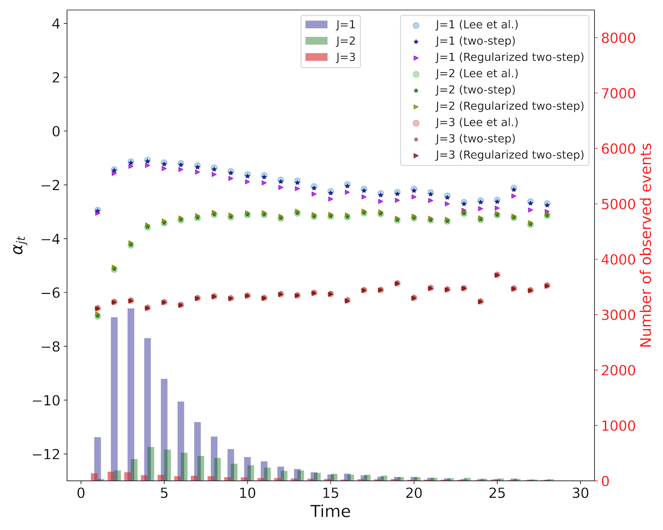
Figure 5: MIMIC dataset - LOS analysis. Results of estimated $\alpha_{jt}$ by the method of Lee et al. (circle), the proposed two-step approach (stars) with no regularization and the proposed approach with lasso (left triangular). Numbers of observed events are shown in blue bars for home discharge ($j=1$), in green bars for further treatment ($j=2$), and in red bars for in-hospital death ($j=3$). lasso estimates are based on $\log\eta_{1}=-5$, $\log\eta_{2}=-9$ and $\log\eta_{3}=-11$.

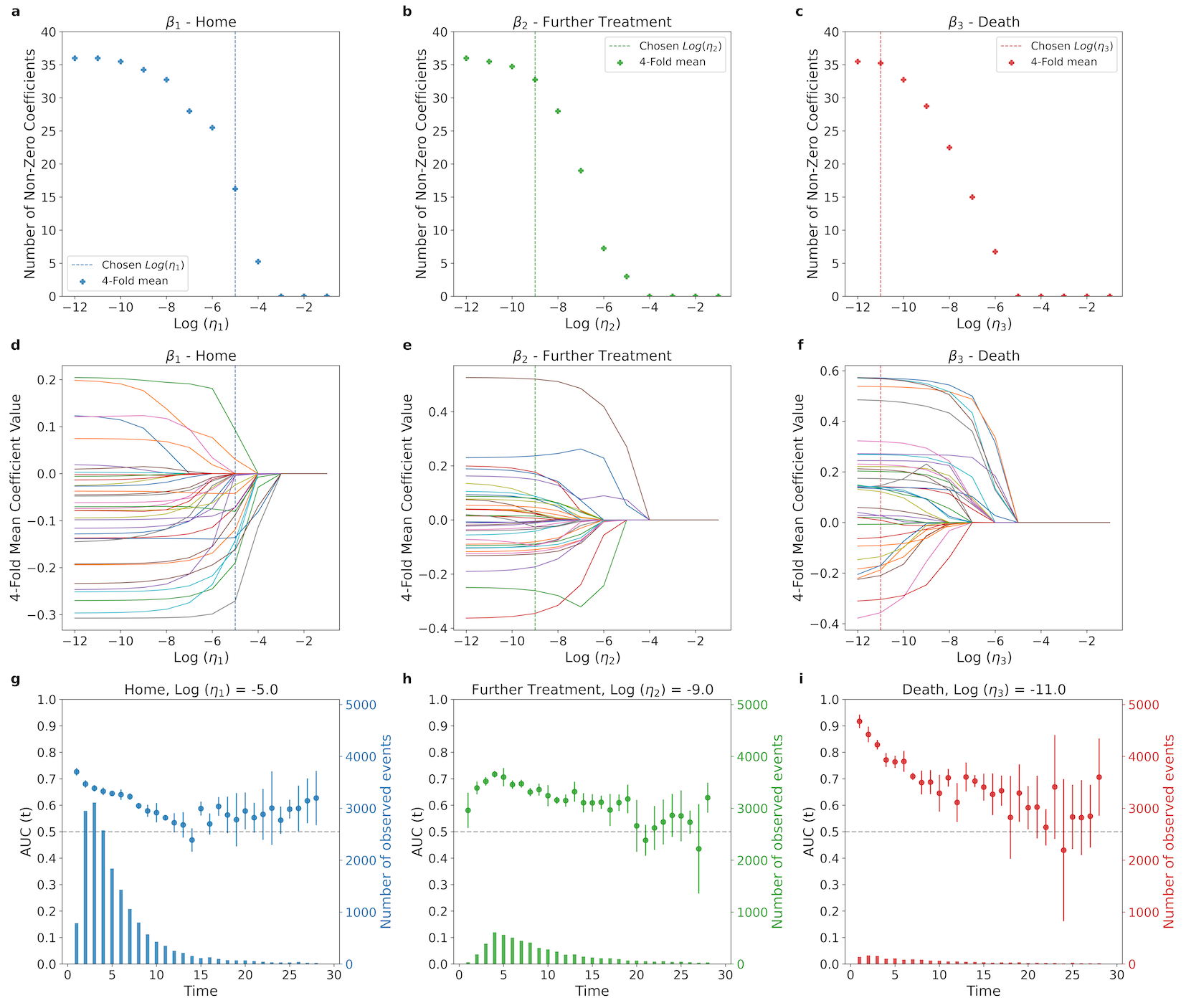
Figure 6: MIMIC dataset - LOS analysis. Regularized regression with 4-fold CV. The selected values of $\eta_{j}$ are shown in dashed-dotted lines on panels a-f. a-c. Number of non-zero coefficients for $j=1,2,3$. d-f. The estimated coefficients, as a function of $\eta_{j}$, $j=1,2,3$. g-i. Mean (and SD bars) of the 4 folds $\widehat{\mbox{AUC}}_{j}(t)$, $j=1,2,3$, for the selected values $\log\eta_{1}=-5$, $\log\eta_{2}=-9$ and $\log\eta_{3}=-11$. The number of observed events of each type is shown by bars.

The data were analysed by three methods: Lee et al., the proposed two-step approach, and the proposed two-step approach with lasso. For the latter, the selection of $\eta_{j}$, $j=1,2,3$, were carried out using 4-fold cross validation, and by maximizing the out-of-sample global AUC. In this application, $\log\eta_{j}$ was allowed to vary from -12 to -1, in steps of 1. The resulting selected values of $\log\eta_{j}$, $j=1,2,3$, were -5, -9 and -11. The results of the three procedures are presented in Tables 6 - 8 and Figures 5 and 6. The parameters’ estimates were similar between Lee et al.’s approach and the two-step procedure without regularization, as expected. Computation time was also similar between Lee et al’s approach and the two-step procedure without regularization with estimation time of 29.5 seconds and 22.1 seconds, respectively.

The global AUCs of the proposed approach without and with lasso penalty were highly similar, $\widehat{\mbox{AUC}}=0.649$ (SD=0.003) and $\widehat{\mbox{AUC}}=0.651$ (SD=0.003) (the SDs in parentheses are based on the 4 folds and do not take into account the variability due to the model estimation). By adding lasso regularization, the number of predictors for each event type was reduced, but the corresponding estimators for $\alpha_{jt}$ remained highly similar. It is worth noting that the estimators of $\alpha_{jt}$ tend to increase as the number of observed events of type $j$ at time $t$ increases.

As evident in Figure 6, the $\mbox{AUC}_{j}(t)$ results for the initial 14 days of hospitalization were higher than for subsequent days. This phenomenon may be attributed to several factors. Firstly, the higher number of observed events during these days may contribute to elevated AUC values. Additionally, the short length of stay can be a consequence of illness severity, with severe cases experiencing short-term in-hospital death and mild cases resulting in short-term discharge, rendering them more easily identifiable. Finally, as treatment progresses, the influence of the initial condition may diminish, while the treatment effect strengthens. This dynamic makes it challenging to differentiate between events occurring during days 14-28 based solely on the covariates measured upon admission.

The integrated cause-specific AUCs were $\widehat{\mbox{AUC}}_{1}=0.642$ (SD=0.002), $\widehat{\mbox{AUC}}_{2}=0.655$ (SD=0.012), and $\widehat{\mbox{AUC}}_{3}=0.740$ (SD=0.006), with a global $\widehat{\mbox{AUC}}=0.651$ (SD=0.003). The integrated cause-specific Brier Scores were $\widehat{\mbox{BS}}_{1}=0.105$ (SD=0.002), $\widehat{\mbox{BS}}_{2}=0.042$ (SD=0.001), and $\widehat{\mbox{BS}}_{3}=0.010$ (SD=0.001), with a global Brier Score of $\widehat{\mbox{BS}}=0.085$ (SD=0.001).

Additional discussion of the results is provided in Appendix F. In this work, we applied the standard lasso regularization. Alternatively, one may apply group-lasso ²⁶, for example, for the features that include multiple dummy variables.

5 Discussion

This work provides a new estimation procedure for a semi-parametric logit-link survival model of discrete time with competing events. Our current deviation from Lee et al. involves a simplification by segregating the estimation procedures for $\alpha_{jt}$ and $\beta_{j}$. This is achieved by substituting the log likelihoods $\log L_{j}$ with conditional log likelihoods $\log L_{j}^{C}(\beta_{j})$, and incorporating loss functions for $\alpha_{jt}$. In Eq. (3), $\alpha_{jt}$ is eliminated, as we stratify by $\tilde{X}$ within each event type $j$. This result remains valid when using both the logit- and log-link functions; however, it does not hold under the complementary log-log model. Our current software is designed to utilize only the logit link.

The hazard models considered in Tutz & Schmid ¹¹, Most et al. ¹² and Schmid & Berger ¹³ are of the form

$$\lambda^{*}_{j}(t|Z)=\frac{\exp(\alpha^{*}_{jt}+Z^{T}\beta^{*}_{j})}{1+\sum_{j^{\prime}=1}^{M}\exp(\alpha^{*}_{j^{\prime}t}+Z^{T}\beta^{*}_{j^{\prime}})}\,\,\,j=1,\ldots,M\,.$$

Namely, the hazard model $\lambda^{*}_{j}$ is a function not only of the parameters associated with the $j$th competing event but also of the parameters related to all other event types. In contrast, the hazard function $\lambda_{j}$ is a function only of the parameters of the $j$th competing event. Both approaches are valid and were presented by Allison ¹. However, as discussed by Allison ¹, models in the spirit of $\lambda_{j}$ provide a natural and direct analogy to the cause-specific hazard function in the context of continuous survival time. Because the discrete-time likelihood cannot be factored into separate components for each of the $M$ types of events, Allison ¹ considered a more tractable formulation. In particular, he explored the generalization of the logistic model $\lambda^{*}_{j}$ which was later adopted by Tutz & Schmid ¹¹, Most et al. ¹² and Schmid & Berger ¹³. Allison ¹ also mentioned that when using $\lambda^{*}_{j}$, the log likelihood for a multinomial logit problem, treating all observed time units for all individuals as separate and independent observations, should be employed. This allows the parameters to be estimated using a binomial logit program (e.g., VGAM). We prefer working with the natural and direct analogy to the cause-specific hazard function in the context of continuous survival time, i.e., with $\lambda_{j}(t|Z)$, as hazard models offer a simpler interpretation. While Lee et al. simplified the estimating procedure, we further streamlined it, particularly in the context of high-dimensional data.

Data and Code Availability Statement

Both estimation methods and the data sampling procedures used in the simulation study were implemented in Python using the PyDTS package ¹⁹. Additionally, we present an example of our approach implemented in R (refer to the Data and Code Availability section). The codes are available under the GNU GPLv3 at the PyDTS package repository https://github.com/tomer1812/pydts/ and at https://github.com/tomer1812/DiscreteTimeSurvivalPenalization. The MIMIC dataset is accessible at https://physionet.org/content/mimiciv/2.0/ and subjected to PhysioNet credentials.

Competing Interests Statement

The authors declare no competing interests.

Table 1: Original and expanded datasets with $M=2$ competing events (Lee et al.)

Original Data				Expanded Data
$i$	$X_{i}$	$\delta_{i}$	$Z_{i}$	$i$	$\tilde{X}_{i}$	$\delta_{1it}$	$\delta_{2it}$	$1-\delta_{1it}-\delta_{2it}$	$Z_{i}$
1	2	1	$Z_{1}$	1	1	0	0	1	$Z_{1}$
				1	2	1	0	0	$Z_{1}$
2	3	2	$Z_{2}$	2	1	0	0	1	$Z_{2}$
				2	2	0	0	1	$Z_{2}$
				2	3	0	1	0	$Z_{2}$
3	3	0	$Z_{3}$	3	1	0	0	1	$Z_{3}$
				3	2	0	0	1	$Z_{3}$
				3	3	0	0	1	$Z_{3}$

Table 2: Overview of simulations settings: number of repetitions is denoted by Rep, Dist stands for the covariates’ distribution, where “indep” and “dep” denote independent and dependent covariates, respectively, “unif” and “normal” denote standard uniform and normal distributions.

			Setting Details					Estimation Methods
No.	Objective	Rep	$n$	$p$	Dist	$M$	$d$	Lee et al.	two-step	Results
1	Performance	200	5000	5	indep, unif	2	30	Yes	Yes	Table 3, Fig 1
2	Performance	200	10000	5	indep, unif	2	30	Yes	Yes	Table 3, Fig 1
3	Performance	200	15000	5	indep, unif	2	30	Yes	Yes	Table 3, Fig 1
4	Performance	200	20000	5	indep, unif	2	30	Yes	Yes	Table 3, Fig 1
5	Performance	200	5000	5	indep, unif	3	30	Yes	Yes	Table S1, Fig S1
6	Performance	200	10000	5	indep, unif	3	30	Yes	Yes	Table S1, Fig S1
7	Performance	200	15000	5	indep, unif	3	30	Yes	Yes	Table S2, Fig S1
8	Performance	200	20000	5	indep, unif	3	30	Yes	Yes	Table S2, Fig S1
9	Performance	200	250	5	indep, unif	2	7	Yes	Yes	Table S3, Fig S2
10	Performance	200	500	5	indep, unif	2	7	Yes	Yes	Table S3, Fig S2
11	Timing	10	20000	10	indep, unif	2	25	Yes	Yes	Fig 2
12	Timing	10	20000	10	indep, unif	2	50	Yes	Yes	Fig 2
13	Timing	10	20000	10	indep, unif	2	75	Yes	Yes	Fig 2
14	Timing	10	20000	10	indep, unif	2	100	Yes	Yes	Fig 2
15	Timing	10	20000	10	indep, unif	2	125	Yes	Yes	Fig 2
16	Timing	10	20000	10	indep, unif	2	150	Yes	Yes	Fig 2
17	Regularization	1	10000	100	indep, normal	2	15	No	Yes	Fig 3
18	Regularization	1	10000	100	dep, normal	2	15	No	Yes	Fig 4
19	Regularization	100	10000	100	indep, normal	2	15	No	Yes	Section 3
20	SIS, SIS-L	100	1000	15000	indep, normal	2	8	No	Yes	Appendix E
21	SIS, SIS-L	100	1000	15000	dep, normal	2	8	No	Yes	Appendix E
22	SIS, SIS-L	100	1000	15000	dep, normal	2	8	No	Yes	Appendix E

Table 3: Simulation results of two competing events. Results of Lee et al. include mean and estimated standard error (Est SE). Results of the proposed two-step approach include mean, estimated SE, empirical SE (Emp SE) and empirical coverage rate (CR) of 95% Wald-type confidence interval.

		True	Lee et al.		Two-Step
$n$	$\beta_{jk}$	Value	Mean	Est SE	Mean	Est SE	Emp SE	CR
5,000	$\beta_{11}$	0.223	0.227	0.094	0.225	0.093	0.104	0.940
	$\beta_{12}$	-1.099	-1.093	0.096	-1.082	0.095	0.104	0.920
	$\beta_{13}$	-1.099	-1.102	0.096	-1.090	0.095	0.105	0.935
	$\beta_{14}$	-0.916	-0.914	0.095	-0.904	0.094	0.092	0.955
	$\beta_{15}$	-0.693	-0.701	0.095	-0.694	0.094	0.099	0.940
	$\beta_{21}$	-0.000	0.004	0.121	0.004	0.120	0.119	0.945
	$\beta_{22}$	-1.099	-1.091	0.124	-1.083	0.123	0.129	0.925
	$\beta_{23}$	-1.386	-1.402	0.125	-1.393	0.125	0.137	0.920
	$\beta_{24}$	-1.099	-1.109	0.124	-1.101	0.123	0.135	0.925
	$\beta_{25}$	-0.693	-0.704	0.122	-0.698	0.121	0.120	0.945
10,000	$\beta_{11}$	0.223	0.226	0.067	0.224	0.066	0.059	0.985
	$\beta_{12}$	-1.099	-1.100	0.068	-1.088	0.067	0.070	0.915
	$\beta_{13}$	-1.099	-1.097	0.068	-1.086	0.067	0.065	0.960
	$\beta_{14}$	-0.916	-0.922	0.067	-0.912	0.067	0.064	0.945
	$\beta_{15}$	-0.693	-0.688	0.067	-0.681	0.066	0.064	0.955
	$\beta_{21}$	-0.000	0.007	0.085	0.007	0.085	0.085	0.955
	$\beta_{22}$	-1.099	-1.107	0.087	-1.100	0.087	0.091	0.930
	$\beta_{23}$	-1.386	-1.389	0.088	-1.380	0.088	0.084	0.965
	$\beta_{24}$	-1.099	-1.085	0.087	-1.077	0.087	0.080	0.965
	$\beta_{25}$	-0.693	-0.690	0.086	-0.685	0.085	0.084	0.945
15,000	$\beta_{11}$	0.223	0.225	0.054	0.222	0.054	0.057	0.945
	$\beta_{12}$	-1.099	-1.103	0.055	-1.092	0.055	0.059	0.940
	$\beta_{13}$	-1.099	-1.100	0.055	-1.089	0.055	0.054	0.950
	$\beta_{14}$	-0.916	-0.925	0.055	-0.916	0.054	0.051	0.970
	$\beta_{15}$	-0.693	-0.686	0.055	-0.679	0.054	0.052	0.950
	$\beta_{21}$	-0.000	-0.000	0.070	-0.000	0.069	0.066	0.955
	$\beta_{22}$	-1.099	-1.092	0.071	-1.085	0.071	0.064	0.955
	$\beta_{23}$	-1.386	-1.381	0.072	-1.372	0.072	0.067	0.955
	$\beta_{24}$	-1.099	-1.101	0.071	-1.094	0.071	0.076	0.940
	$\beta_{25}$	-0.693	-0.689	0.070	-0.684	0.070	0.071	0.945
20,000	$\beta_{11}$	0.223	0.220	0.047	0.217	0.047	0.046	0.935
	$\beta_{12}$	-1.099	-1.099	0.048	-1.088	0.048	0.044	0.965
	$\beta_{13}$	-1.099	-1.098	0.048	-1.087	0.048	0.046	0.940
	$\beta_{14}$	-0.916	-0.920	0.048	-0.910	0.047	0.041	0.980
	$\beta_{15}$	-0.693	-0.690	0.047	-0.682	0.047	0.046	0.945
	$\beta_{21}$	-0.000	0.003	0.060	0.003	0.060	0.065	0.930
	$\beta_{22}$	-1.099	-1.095	0.062	-1.088	0.061	0.066	0.940
	$\beta_{23}$	-1.386	-1.394	0.063	-1.385	0.062	0.057	0.980
	$\beta_{24}$	-1.099	-1.096	0.062	-1.089	0.061	0.061	0.950
	$\beta_{25}$	-0.693	-0.700	0.061	-0.695	0.061	0.056	0.970

Table 4: MIMIC dataset. Summary of covariates of overall sample, among censored observations, and by event type: in-hospital death (Death), discharged to another medical facility (Another Facility), and discharge to home (Home).

				Event Type
		Overall	Censored	Death	Another Facility	Home
$n$		25170	894	1540	5379	17357
Sex (%)	Female	12291 (48.8)	373 (41.7)	695 (45.1)	2865 (53.3)	8358 (48.2)
	Male	12879 (51.2)	521 (58.3)	845 (54.9)	2514 (46.7)	8999 (51.8)
Age, mean (SD)		64.1 (17.9)	58.4 (16.5)	72.7 (14.5)	73.3 (15.7)	60.8 (17.6)
Race (%)	Asian	1035 (4.1)	27 (3.0)	76 (4.9)	165 (3.1)	767 (4.4)
	Black	3543 (14.1)	154 (17.2)	197 (12.8)	741 (13.8)	2451 (14.1)
	Hispanic	1326 (5.3)	53 (5.9)	53 (3.4)	180 (3.3)	1040 (6.0)
	White	17595 (69.9)	595 (66.6)	1072 (69.6)	3977 (73.9)	11951 (68.9)
	Other	1671 (6.6)	65 (7.3)	142 (9.2)	316 (5.9)	1148 (6.6)
Insurance (%)	Medicaid	1423 (5.7)	86 (9.6)	66 (4.3)	222 (4.1)	1049 (6.0)
	Medicare	10609 (42.1)	316 (35.3)	843 (54.7)	3253 (60.5)	6197 (35.7)
	Other	13138 (52.2)	492 (55.0)	631 (41.0)	1904 (35.4)	10111 (58.3)
Marital Status (%)	Divorced	2043 (8.1)	94 (10.5)	121 (7.9)	464 (8.6)	1364 (7.9)
	Married	11289 (44.9)	329 (36.8)	751 (48.8)	1853 (34.4)	8356 (48.1)
	Single	8414 (33.4)	403 (45.1)	386 (25.1)	1729 (32.1)	5896 (34.0)
	Widowed	3424 (13.6)	68 (7.6)	282 (18.3)	1333 (24.8)	1741 (10.0)
Direct Emergency (%)	No	22398 (89.0)	790 (88.4)	1413 (91.8)	4924 (91.5)	15271 (88.0)
	Yes	2772 (11.0)	104 (11.6)	127 (8.2)	455 (8.5)	2086 (12.0)
Night Admission (%)	No	11604 (46.1)	404 (45.2)	736 (47.8)	2414 (44.9)	8050 (46.4)
	Yes	13566 (53.9)	490 (54.8)	804 (52.2)	2965 (55.1)	9307 (53.6)
Previous Admission this Month (%)	No	23138 (91.9)	795 (88.9)	1318 (85.6)	4821 (89.6)	16204 (93.4)
	Yes	2032 (8.1)	99 (11.1)	222 (14.4)	558 (10.4)	1153 (6.6)
Admissions Number (%)	1	15471 (61.5)	503 (56.3)	798 (51.8)	3005 (55.9)	11165 (64.3)
	2	4121 (16.4)	151 (16.9)	283 (18.4)	926 (17.2)	2761 (15.9)
	3+	5578 (22.2)	240 (26.8)	459 (29.8)	1448 (26.9)	3431 (19.8)
LOS (days), mean (SD)		7.0 (6.1)	21.7 (11.6)	8.5 (6.9)	9.0 (5.8)	5.5 (4.3)

Table 5: MIMIC dataset. Summary of covariates of overall sample, among censored observations, and by event type: in-hospital death (Death), discharged to another medical facility (Another Facility), and discharge to home (Home). MCH: mean cell hemoglobin. MCHC: mean cell hemoglobin concentration. MCV: mean corpuscular volume. RDW: red blood cell Distribution Width.

				Event Type
		Overall	Censored	Death	Another Facility	Home
$n$		25170	894	1540	5379	17357
Anion Gap (%)	Abnormal	2305 (9.2)	110 (12.3)	401 (26.0)	543 (10.1)	1251 (7.2)
	Normal	22865 (90.8)	784 (87.7)	1139 (74.0)	4836 (89.9)	16106 (92.8)
Bicarbonate (%)	Abnormal	6135 (24.4)	300 (33.6)	832 (54.0)	1494 (27.8)	3509 (20.2)
	Normal	19035 (75.6)	594 (66.4)	708 (46.0)	3885 (72.2)	13848 (79.8)
Calcium Total (%)	Abnormal	7326 (29.1)	365 (40.8)	756 (49.1)	1823 (33.9)	4382 (25.2)
	Normal	17844 (70.9)	529 (59.2)	784 (50.9)	3556 (66.1)	12975 (74.8)
Chloride (%)	Abnormal	4848 (19.3)	255 (28.5)	555 (36.0)	1322 (24.6)	2716 (15.6)
	Normal	20322 (80.7)	639 (71.5)	985 (64.0)	4057 (75.4)	14641 (84.4)
Creatinine (%)	Abnormal	7124 (28.3)	323 (36.1)	893 (58.0)	1945 (36.2)	3963 (22.8)
	Normal	18046 (71.7)	571 (63.9)	647 (42.0)	3434 (63.8)	13394 (77.2)
Glucose (%)	Abnormal	16426 (65.3)	635 (71.0)	1211 (78.6)	3674 (68.3)	10906 (62.8)
	Normal	8744 (34.7)	259 (29.0)	329 (21.4)	1705 (31.7)	6451 (37.2)
Magnesium (%)	Abnormal	2220 (8.8)	99 (11.1)	234 (15.2)	517 (9.6)	1370 (7.9)
	Normal	22950 (91.2)	795 (88.9)	1306 (84.8)	4862 (90.4)	15987 (92.1)
Phosphate (%)	Abnormal	6962 (27.7)	313 (35.0)	663 (43.1)	1510 (28.1)	4476 (25.8)
	Normal	18208 (72.3)	581 (65.0)	877 (56.9)	3869 (71.9)	12881 (74.2)
Potassium (%)	Abnormal	2109 (8.4)	110 (12.3)	260 (16.9)	520 (9.7)	1219 (7.0)
	Normal	23061 (91.6)	784 (87.7)	1280 (83.1)	4859 (90.3)	16138 (93.0)
Sodium (%)	Abnormal	2947 (11.7)	171 (19.1)	415 (26.9)	845 (15.7)	1516 (8.7)
	Normal	22223 (88.3)	723 (80.9)	1125 (73.1)	4534 (84.3)	15841 (91.3)
Urea Nitrogen (%)	Abnormal	10032 (39.9)	413 (46.2)	1059 (68.8)	2849 (53.0)	5711 (32.9)
	Normal	15138 (60.1)	481 (53.8)	481 (31.2)	2530 (47.0)	11646 (67.1)
Hematocrit (%)	Abnormal	17319 (68.8)	691 (77.3)	1250 (81.2)	4111 (76.4)	11267 (64.9)
	Normal	7851 (31.2)	203 (22.7)	290 (18.8)	1268 (23.6)	6090 (35.1)
Hemoglobin (%)	Abnormal	18355 (72.9)	735 (82.2)	1319 (85.6)	4320 (80.3)	11981 (69.0)
	Normal	6815 (27.1)	159 (17.8)	221 (14.4)	1059 (19.7)	5376 (31.0)
MCH (%)	Abnormal	6559 (26.1)	306 (34.2)	454 (29.5)	1488 (27.7)	4311 (24.8)
	Normal	18611 (73.9)	588 (65.8)	1086 (70.5)	3891 (72.3)	13046 (75.2)
MCHC (%)	Abnormal	7762 (30.8)	313 (35.0)	634 (41.2)	2033 (37.8)	4782 (27.6)
	Normal	17408 (69.2)	581 (65.0)	906 (58.8)	3346 (62.2)	12575 (72.4)
MCV (%)	Abnormal	5106 (20.3)	243 (27.2)	418 (27.1)	1229 (22.8)	3216 (18.5)
	Normal	20064 (79.7)	651 (72.8)	1122 (72.9)	4150 (77.2)	14141 (81.5)
Platelet Count (%)	Abnormal	7280 (28.9)	364 (40.7)	688 (44.7)	1618 (30.1)	4610 (26.6)
	Normal	17890 (71.1)	530 (59.3)	852 (55.3)	3761 (69.9)	12747 (73.4)
RDW (%)	Abnormal	7280 (28.9)	377 (42.2)	870 (56.5)	2016 (37.5)	4017 (23.1)
	Normal	17890 (71.1)	517 (57.8)	670 (43.5)	3363 (62.5)	13340 (76.9)
Red Blood Cells (%)	Abnormal	19170 (76.2)	732 (81.9)	1341 (87.1)	4478 (83.2)	12619 (72.7)
	Normal	6000 (23.8)	162 (18.1)	199 (12.9)	901 (16.8)	4738 (27.3)
White Blood Cells (%)	Abnormal	10013 (39.8)	466 (52.1)	1012 (65.7)	2320 (43.1)	6215 (35.8)
	Normal	15157 (60.2)	428 (47.9)	528 (34.3)	3059 (56.9)	11142 (64.2)

Table 6: MIMIC dataset - LOS analysis: Estimated regression coefficients of event type discharge to home, $J=1$.

		Lee et al.	Two-Step	Two-Step & lasso
		Estimate (SE)	Estimate (SE)	Estimate (SE)
Admissions Number	2	0.000 (0.024)	0.003 (0.022)	0.000 (0.000)
	3+	-0.032 (0.023)	-0.027 (0.022)	0.000 (0.000)
Anion Gap	Abnormal	-0.137 (0.032)	-0.128 (0.030)	0.000 (0.000)
Bicarbonate	Abnormal	-0.208 (0.021)	-0.194 (0.020)	-0.119 (0.019)
Calcium Total	Abnormal	-0.291 (0.020)	-0.270 (0.019)	-0.190 (0.018)
Chloride	Abnormal	-0.148 (0.024)	-0.137 (0.023)	-0.071 (0.021)
Creatinine	Abnormal	-0.103 (0.024)	-0.098 (0.023)	-0.072 (0.021)
Direct Emergency	Yes	-0.011 (0.026)	-0.014 (0.024)	0.000 (0.000)
Ethnicity	Black	0.006 (0.046)	0.009 (0.042)	0.000 (0.000)
	Hispanic	0.132 (0.053)	0.120 (0.048)	0.000 (0.000)
	Other	-0.162 (0.051)	-0.146 (0.047)	0.000 (0.000)
	White	-0.031 (0.041)	-0.026 (0.038)	0.000 (0.000)
Glucose	Abnormal	-0.215 (0.018)	-0.192 (0.016)	-0.088 (0.016)
Hematocrit	Abnormal	-0.042 (0.032)	-0.037 (0.029)	-0.042 (0.029)
Hemoglobin	Abnormal	-0.080 (0.033)	-0.071 (0.030)	-0.081 (0.030)
Insurance	Medicare	0.138 (0.039)	0.125 (0.036)	0.000 (0.000)
	Other	0.219 (0.036)	0.200 (0.033)	0.030 (0.016)
MCH	Abnormal	-0.002 (0.023)	-0.002 (0.022)	0.000 (0.000)
MCHC	Abnormal	-0.128 (0.019)	-0.116 (0.018)	-0.003 (0.017)
MCV	Abnormal	-0.048 (0.026)	-0.045 (0.024)	0.000 (0.000)
Magnesium	Abnormal	-0.080 (0.030)	-0.074 (0.028)	0.000 (0.000)
Marital Status	Married	0.224 (0.032)	0.205 (0.030)	0.093 (0.016)
	Single	-0.087 (0.033)	-0.079 (0.031)	0.000 (0.000)
	Widowed	0.026 (0.040)	0.020 (0.037)	0.000 (0.000)
Night Admission	Yes	0.081 (0.017)	0.075 (0.016)	0.000 (0.000)
Phosphate	Abnormal	-0.052 (0.019)	-0.048 (0.018)	0.000 (0.000)
Platelet Count	Abnormal	-0.068 (0.019)	-0.062 (0.018)	0.000 (0.000)
Potassium	Abnormal	-0.103 (0.032)	-0.095 (0.030)	0.000 (0.000)
RDW	Abnormal	-0.327 (0.021)	-0.308 (0.020)	-0.271 (0.019)
Recent Admission	Yes	-0.262 (0.035)	-0.247 (0.033)	-0.001 (0.027)
Red Blood Cells	Abnormal	-0.089 (0.027)	-0.078 (0.024)	-0.024 (0.025)
Sex	Female	-0.007 (0.018)	-0.006 (0.016)	0.000 (0.000)
Sodium	Abnormal	-0.312 (0.030)	-0.297 (0.029)	-0.142 (0.026)
Standardized Age		-0.260 (0.011)	-0.234 (0.010)	-0.162 (0.009)
Urea Nitrogen	Abnormal	-0.148 (0.022)	-0.139 (0.020)	-0.136 (0.020)
White Blood Cells	Abnormal	-0.276 (0.018)	-0.252 (0.016)	-0.159 (0.016)

Table 7: MIMIC dataset - LOS analysis: Estimated regression coefficients of event type discharged to another facility, $J=2$.

		Lee et al.	Two-Step	Two-Step & lasso
		Estimate (SE)	Estimate (SE)	Estimate (SE)
Admissions Number	2	0.108 (0.041)	0.107 (0.040)	0.087 (0.038)
	3+	0.194 (0.037)	0.190 (0.036)	0.169 (0.034)
Anion Gap	Abnormal	-0.006 (0.048)	-0.006 (0.047)	0.000 (0.002)
Bicarbonate	Abnormal	-0.121 (0.033)	-0.117 (0.032)	-0.110 (0.032)
Calcium Total	Abnormal	-0.098 (0.031)	-0.094 (0.031)	-0.088 (0.030)
Chloride	Abnormal	0.016 (0.036)	0.015 (0.035)	0.000 (0.002)
Creatinine	Abnormal	-0.199 (0.036)	-0.191 (0.035)	-0.173 (0.035)
Direct Emergency	Yes	-0.373 (0.052)	-0.363 (0.050)	-0.345 (0.050)
Ethnicity	Black	0.084 (0.090)	0.079 (0.088)	0.028 (0.086)
	Hispanic	-0.068 (0.111)	-0.070 (0.108)	-0.088 (0.106)
	Other	0.026 (0.099)	0.022 (0.097)	-0.006 (0.095)
	White	0.144 (0.082)	0.138 (0.081)	0.094 (0.079)
Glucose	Abnormal	-0.138 (0.031)	-0.132 (0.030)	-0.126 (0.030)
Hematocrit	Abnormal	0.038 (0.057)	0.039 (0.055)	0.032 (0.055)
Hemoglobin	Abnormal	0.018 (0.062)	0.015 (0.060)	0.005 (0.059)
Insurance	Medicare	0.237 (0.075)	0.230 (0.074)	0.238 (0.073)
	Other	-0.094 (0.074)	-0.091 (0.072)	-0.081 (0.072)
MCH	Abnormal	0.042 (0.038)	0.040 (0.037)	0.019 (0.031)
MCHC	Abnormal	-0.010 (0.031)	-0.011 (0.030)	0.000 (0.003)
MCV	Abnormal	-0.020 (0.041)	-0.019 (0.039)	0.000 (0.003)
Magnesium	Abnormal	-0.039 (0.048)	-0.038 (0.047)	-0.025 (0.046)
Marital Status	Married	-0.254 (0.054)	-0.249 (0.053)	-0.262 (0.052)
	Single	0.209 (0.054)	0.200 (0.053)	0.176 (0.052)
	Widowed	0.175 (0.058)	0.163 (0.056)	0.149 (0.056)
Night Admission	Yes	0.056 (0.029)	0.054 (0.028)	0.047 (0.028)
Phosphate	Abnormal	-0.042 (0.033)	-0.040 (0.032)	-0.034 (0.031)
Platelet Count	Abnormal	-0.130 (0.032)	-0.125 (0.031)	-0.118 (0.031)
Potassium	Abnormal	0.042 (0.048)	0.042 (0.047)	0.023 (0.047)
RDW	Abnormal	-0.107 (0.033)	-0.104 (0.032)	-0.093 (0.031)
Recent Admission	Yes	-0.021 (0.051)	-0.023 (0.049)	0.000 (0.004)
Red Blood Cells	Abnormal	0.083 (0.052)	0.079 (0.050)	0.073 (0.050)
Sex	Female	0.090 (0.031)	0.088 (0.030)	0.078 (0.030)
Sodium	Abnormal	-0.056 (0.042)	-0.056 (0.041)	-0.039 (0.038)
Standardized Age		0.536 (0.021)	0.525 (0.021)	0.519 (0.021)
Urea Nitrogen	Abnormal	0.100 (0.035)	0.095 (0.034)	0.077 (0.034)
White Blood Cells	Abnormal	-0.107 (0.029)	-0.103 (0.028)	-0.099 (0.028)

Table 8: MIMIC dataset - LOS analysis: Estimated regression coefficients of event type in-hospital death, $J=3$.

		Lee et al.	Two-Step	Two-Step & lasso
		Estimate (SE)	Estimate (SE)	Estimate (SE)
Admissions Number	2	0.147 (0.074)	0.147 (0.073)	0.140 (0.074)
	3+	0.142 (0.069)	0.140 (0.068)	0.134 (0.068)
Anion Gap	Abnormal	0.582 (0.064)	0.573 (0.064)	0.571 (0.064)
Bicarbonate	Abnormal	0.543 (0.056)	0.537 (0.056)	0.535 (0.056)
Calcium Total	Abnormal	0.204 (0.054)	0.204 (0.054)	0.203 (0.054)
Chloride	Abnormal	0.147 (0.059)	0.143 (0.058)	0.142 (0.058)
Creatinine	Abnormal	0.273 (0.067)	0.271 (0.067)	0.271 (0.067)
Direct Emergency	Yes	-0.318 (0.096)	-0.311 (0.095)	-0.302 (0.095)
Ethnicity	Black	-0.236 (0.140)	-0.235 (0.139)	-0.203 (0.140)
	Hispanic	-0.395 (0.183)	-0.393 (0.181)	-0.351 (0.181)
	Other	0.145 (0.147)	0.133 (0.145)	0.155 (0.146)
	White	-0.156 (0.123)	-0.157 (0.122)	-0.130 (0.123)
Glucose	Abnormal	0.215 (0.064)	0.212 (0.063)	0.208 (0.063)
Hematocrit	Abnormal	-0.198 (0.108)	-0.194 (0.107)	-0.165 (0.108)
Hemoglobin	Abnormal	0.024 (0.122)	0.023 (0.121)	0.003 (0.121)
Insurance	Medicare	-0.224 (0.136)	-0.225 (0.135)	-0.171 (0.138)
	Other	-0.242 (0.133)	-0.240 (0.132)	-0.188 (0.135)
MCH	Abnormal	-0.066 (0.070)	-0.066 (0.069)	-0.057 (0.069)
MCHC	Abnormal	0.027 (0.056)	0.029 (0.055)	0.027 (0.055)
MCV	Abnormal	0.060 (0.072)	0.061 (0.071)	0.055 (0.071)
Magnesium	Abnormal	0.329 (0.073)	0.324 (0.072)	0.320 (0.072)
Marital Status	Married	0.156 (0.102)	0.154 (0.101)	0.127 (0.061)
	Single	0.026 (0.107)	0.027 (0.106)	0.000 (0.008)
	Widowed	0.047 (0.115)	0.048 (0.114)	0.020 (0.084)
Night Admission	Yes	-0.096 (0.053)	-0.093 (0.052)	-0.089 (0.052)
Phosphate	Abnormal	0.178 (0.056)	0.176 (0.055)	0.174 (0.055)
Platelet Count	Abnormal	0.235 (0.054)	0.232 (0.054)	0.229 (0.054)
Potassium	Abnormal	0.227 (0.072)	0.221 (0.071)	0.221 (0.071)
RDW	Abnormal	0.492 (0.058)	0.486 (0.058)	0.483 (0.058)
Recent Admission	Yes	0.250 (0.083)	0.242 (0.082)	0.242 (0.082)
Red Blood Cells	Abnormal	0.142 (0.105)	0.140 (0.104)	0.130 (0.104)
Sex	Female	-0.011 (0.057)	-0.008 (0.057)	-0.005 (0.057)
Sodium	Abnormal	0.276 (0.064)	0.270 (0.063)	0.268 (0.063)
Standardized Age		0.580 (0.041)	0.574 (0.040)	0.568 (0.040)
Urea Nitrogen	Abnormal	0.141 (0.070)	0.141 (0.070)	0.141 (0.070)
White Blood Cells	Abnormal	0.579 (0.056)	0.571 (0.056)	0.568 (0.055)

Appendix A. Asymptotic Results

Let us assume that as $n\rightarrow\infty$, both $d$ and $M$ are finite fixed values, and the vectors of covariates $Z$ are bounded. Additionally, it is assumed that $\Pr(Y_{.}(t)\geq 1)>0$ for all $t=1,\ldots,d$. We denote the true regression of coefficient values as $\beta^{o}_{j}$. Assume that $\alpha_{jt}$, $j=1,\ldots,M$, $t=1,\ldots,d$, lie in a compact convex set $\mathcal{A}$ that includes an open neighborhood around each true value $\alpha^{o}_{jt}$.

For each $(j,t)$, $j=1,\dots,M$, $t=1,\ldots,d$, minimizing

$$\left\{\frac{1}{Y.(t)}\sum_{i=1}^{n}I(X_{i}\geq t)\frac{\exp(a+Z_{i}^{T}\widehat{\beta}_{j})}{1+\exp(a+Z_{i}^{T}\widehat{\beta}_{j})}-\frac{N_{j}(t)}{Y.(t)}\right\}^{2}$$

as a function of $a$ is equivalent to solving

$$2\left\{\frac{1}{Y.(t)}\sum_{i=1}^{n}I(X_{i}\geq t)\frac{\exp(a+Z_{i}^{T}\widehat{\beta}_{j})}{1+\exp(a+Z_{i}^{T}\widehat{\beta}_{j})}-\frac{N_{j}(t)}{Y.(t)}\right\}\frac{\partial}{\partial a}\frac{1}{Y.(t)}\sum_{i=1}^{n}I(X_{i}\geq t)\frac{\exp(a+Z_{i}^{T}\widehat{\beta}_{j})}{1+\exp(a+Z_{i}^{T}\widehat{\beta}_{j})}=0$$

or alternatively solving

$$\frac{1}{n}\sum_{i=1}^{n}\left\{I(X_{i}\geq t)\frac{\exp(a+Z_{i}^{T}\widehat{\beta}_{j})}{1+\exp(a+Z_{i}^{T}\widehat{\beta}_{j})}-I(X_{i}=t,J_{i}=j)\right\}=0\,.$$

Define

$$U_{n}(\alpha_{jt})=\frac{1}{n}\sum_{i=1}^{n}\left\{I(X_{i}\geq t)\frac{\exp(a+Z_{i}^{T}\widehat{\beta}_{j})}{1+\exp(a+Z_{i}^{T}\widehat{\beta}_{j})}-I(X_{i}=t,J_{i}=j)\right\}$$

and

$$\widetilde{U}_{n}(\alpha_{jt})=\frac{1}{n}\sum_{i=1}^{n}\left\{I(X_{i}\geq t)\frac{\exp(a+Z_{i}^{T}{\beta}^{o}_{j})}{1+\exp(a+Z_{i}^{T}{\beta}^{o}_{j})}-I(X_{i}=t,J_{i}=j)\right\}\,.$$

Then,

$$U_{n}(\alpha_{jt})-\widetilde{U}_{n}(\alpha_{jt})=\frac{1}{n}\sum_{i=1}^{n}I(X_{i}\geq t)\left\{\frac{\exp(a+Z_{i}^{T}\widehat{\beta}_{j})}{1+\exp(a+Z_{i}^{T}\widehat{\beta}_{j})}-\frac{\exp(a+Z_{i}^{T}{\beta}^{o}_{j})}{1+\exp(a+Z_{i}^{T}{\beta}^{o}_{j})}\right\}\,.$$

Taking a first-order Taylor expansion about $\beta^{o}_{j}$ gives

$$U_{n}(\alpha_{jt})-\widetilde{U}_{n}(\alpha_{jt})=\frac{1}{n}\sum_{i=1}^{n}I(X_{i}\geq t)\frac{\partial}{\partial\beta^{o}_{j}}\frac{\exp(a+Z_{i}^{T}{\beta}^{o}_{j})}{1+\exp(a+Z_{i}^{T}{\beta}^{o}_{j})}(\widehat{\beta}_{j}-\beta^{o}_{j})+o_{p}(1)\,.$$

Since $||\widehat{\beta}_{j}-\beta^{o}_{j}||_{2}=o_{p}(1)$ as $n\rightarrow\infty$, where $||\cdot||_{2}$ denotes the $l_{2}$ norm, and since $U_{n}(\alpha_{jt})-\widetilde{U}_{n}(\alpha_{jt})$ is continuous in $\widehat{\beta}_{j}$, then by the continuous mapping theorem and Slutsky theorem, $\sup_{\alpha_{jt}\in\mathcal{A}}|U_{n}(\alpha_{jt})-\widetilde{U}_{n}(\alpha_{jt})|=o_{p}(1)$. Finally, since

$$E(T_{i}=t,J_{i}=j|T_{i}\geq t)=\frac{\exp(a+Z_{i}^{T}{\beta}_{j})}{1+\exp(a+Z_{i}^{T}{\beta}_{j})}\,,$$

consistency and asymptotic normality of each $\widehat{\alpha}_{jt}$, as $n\rightarrow\infty$, follows by standard theory of moment estimators ²⁷ applied for $\widetilde{U}_{n}(\alpha_{jt})$.

Appendix B. ROC-AUC and Brier Score for Discrete Time Setting with Competing Risks

Let

$$\pi_{ij}(t)=\widehat{\Pr}(T_{i}=t,J_{i}=j\mid Z_{i})=\widehat{\lambda}_{j}(t\mid Z_{i})\widehat{S}(t-1\mid Z_{i})$$

and

$$D_{ij}(t)=I(T_{i}=t,J_{i}=j)\,.$$

The cause-specific incidence/dynamic area under the receiver operating characteristics curve (AUC) is defined and estimated in the spirit of Heagerty and Zheng (2005) ²⁸ and Blanche et al. (2015) ²⁹ as the probability of a random observation with observed event $j$ at time $t$ having a higher risk prediction for cause $j$ than a randomly selected observation $m$, at risk at time $t$, without the observed event $j$ at time $t$. Namely,

$$\mbox{AUC}_{j}(t)=\Pr(\pi_{ij}(t)>\pi_{mj}(t)\mid D_{ij}(t)=1,D_{mj}(t)=0,T_{m}\geq t)\,.$$

In the presence of censored data and under the assumption that the censoring is independent of the failure time and observed covariates, an inverse probability censoring weighting (IPCW) estimator of $\mbox{AUC}_{j}(t)$ becomes

$$\widehat{\mbox{AUC}}_{j}(t) = \frac{\sum_{i=1}^{n}\sum_{m=1}^{n}D_{ij}(t)(1-D_{mj}(t))I(X_{m}\geq t)W_{ij}(t)W_{mj}(t)\{I(\pi_{ij}(t)>\pi_{mj}(t))+0.5I(\pi_{ij}(t)=\pi_{mj}(t))\}}{\sum_{i=1}^{n}\sum_{m=1}^{n}D_{ij}(t)(1-D_{mj}(t))I(X_{m}\geq t)W_{ij}(t)W_{mj}(t)}$$

$$= \frac{\sum_{i=1}^{n}\sum_{m=1}^{n}D_{ij}(t)(1-D_{mj}(t))I(X_{m}\geq t)\{I(\pi_{ij}(t)>\pi_{mj}(t))+0.5I(\pi_{ij}(t)=\pi_{mj}(t))\}}{\sum_{i=1}^{n}\sum_{m=1}^{n}D_{ij}(t)(1-D_{mj}(t))I(X_{m}\geq t)}$$

where

$$W_{ij}(t) = \frac{D_{ij}(t)}{\widehat{G}_{C}(T_{i})}+I(X_{i}\geq t)\frac{1-D_{ij}(t)}{\widehat{G}_{C}(t)}=\frac{D_{ij}(t)}{\widehat{G}_{C}(t)}+I(X_{i}\geq t)\frac{1-D_{ij}(t)}{\widehat{G}_{C}(t)}$$

$$= I(X_{i}\geq t)/\widehat{G}_{C}(t)$$

and $\widehat{G}_{C}(\cdot)$ is the estimated survival function of the censoring (e.g., the Kaplan-Meier estimator). Interestingly, the IPCWs have no effect on $\widehat{\mbox{AUC}}_{j}(t)$. An integrated cause-specific AUC can be estimated as a weighted sum by

$$\widehat{\mbox{AUC}}_{j}=\sum_{t}\widehat{\mbox{AUC}}_{j}(t)w_{j}(t)\,,$$

and we adopt a simple data-driven weight function of the form

$$w_{j}(t)=\frac{N_{j}(t)}{\sum_{t}N_{j}(t)}\,.$$

A global AUC can be defined as

$$\widehat{\mbox{AUC}}=\sum_{j}\widehat{\mbox{AUC}}_{j}v_{j}$$

where

$$v_{j}=\frac{\sum_{t}N_{j}(t)}{\sum_{j=1}^{M}\sum_{t}N_{j}(t)}\,.$$

Another well-known performance measure is the Brier Score (BS). In the spirit of Blanche et al. (2015) ²⁹ we define

$$\widehat{\mbox{BS}}_{j}(t)=\frac{1}{Y_{\cdot}(t)}{\sum_{i=1}^{n}W_{ij}(t)\left(D_{ij}(t)-\pi_{ij}(t)\right)^{2}}\,.$$

An integrated cause-specific BS can be estimated by the weighted sum

$$\widehat{\mbox{BS}}_{j}=\sum_{t}\widehat{\mbox{BS}}_{j}(t)w_{j}(t)$$

and an estimated global BS is given by

$$\widehat{\mbox{BS}}=\sum_{j}\widehat{\mbox{BS}}_{j}v_{j}\,.$$

Appendix C. Simulation Results of Three Competing Events

We considered sample sizes of $n=5,000,10,000,15,000$ and $20,000$. The vector of covariates $Z$ is of $p=5$ dimension, and each covariate was sampled from a standard uniform distribution. For each observation, based on the sampled covariates $Z$ and the true model of Eq.( 1), the event type was sampled, and then the failure time, with $d=30$. The parameters’ values were set to be $\alpha_{1t}=-2.2-0.1\log t$, $\alpha_{2t}=-2.3-0.1\log t$, and $\alpha_{3t}=-2.4-0.1\log t$ $t=1,\ldots,30$, $\beta_{1}=-(\log 2.5,\log 1.5,\log 0.8,\log 3,\log 2)$, $\beta_{2}=-(\log 0.8,\log 3,\log 2.8,\log 2.2,\log 1.5)$, and $\beta_{3}=-(\log 1.8,\log 0.8,\log 2.5,\log 1.2,\log 3)$. Finally, the censoring times were sampled from a discrete uniform distribution with probability 0.01 at each $t\leq 30$. The simulation results are based on 200 repetitions of each setting.

Table S1 : Simulation results of three competing events. Results of Lee et al. include mean and estimated standard error (Est SE). Results of the proposed two-step approach include mean, estimated SE, empirical SE (Emp SE) and empirical coverage rate (CR) of 95% Wald-type confidence interval.

		True	Lee et al.		Two-Step
$n$	$\beta_{jk}$	Value	Mean	Est SE	Mean	Est SE	Emp SE	CR
5,000	$\beta_{11}$	-0.916	-0.929	0.098	-0.917	0.097	0.090	0.965
	$\beta_{12}$	-0.405	-0.410	0.097	-0.404	0.096	0.097	0.950
	$\beta_{13}$	0.223	0.224	0.098	0.221	0.097	0.098	0.935
	$\beta_{14}$	-1.099	-1.110	0.098	-1.095	0.097	0.110	0.900
	$\beta_{15}$	-0.693	-0.697	0.098	-0.687	0.096	0.099	0.935
	$\beta_{21}$	0.223	0.246	0.107	0.243	0.105	0.109	0.945
	$\beta_{22}$	-1.099	-1.094	0.108	-1.081	0.107	0.105	0.945
	$\beta_{23}$	-1.030	-1.035	0.107	-1.023	0.106	0.111	0.940
	$\beta_{24}$	-0.788	-0.783	0.107	-0.773	0.105	0.103	0.950
	$\beta_{25}$	-0.405	-0.416	0.107	-0.411	0.105	0.095	0.965
	$\beta_{31}$	-0.588	-0.592	0.099	-0.584	0.098	0.106	0.940
	$\beta_{32}$	0.223	0.237	0.099	0.234	0.098	0.098	0.970
	$\beta_{33}$	-0.916	-0.925	0.100	-0.913	0.099	0.107	0.930
	$\beta_{34}$	-0.182	-0.183	0.099	-0.180	0.098	0.110	0.905
	$\beta_{35}$	-1.099	-1.108	0.100	-1.094	0.099	0.099	0.945
10,000	$\beta_{11}$	-0.916	-0.922	0.069	-0.909	0.068	0.067	0.965
	$\beta_{12}$	-0.405	-0.412	0.068	-0.406	0.068	0.067	0.950
	$\beta_{13}$	0.223	0.221	0.069	0.218	0.068	0.064	0.955
	$\beta_{14}$	-1.099	-1.093	0.069	-1.078	0.068	0.067	0.925
	$\beta_{15}$	-0.693	-0.691	0.069	-0.681	0.068	0.070	0.940
	$\beta_{21}$	0.223	0.222	0.075	0.220	0.075	0.080	0.945
	$\beta_{22}$	-1.099	-1.104	0.076	-1.091	0.075	0.076	0.965
	$\beta_{23}$	-1.030	-1.030	0.076	-1.019	0.075	0.074	0.940
	$\beta_{24}$	-0.788	-0.789	0.075	-0.780	0.075	0.070	0.950
	$\beta_{25}$	-0.405	-0.412	0.075	-0.407	0.074	0.077	0.920
	$\beta_{31}$	-0.588	-0.587	0.070	-0.579	0.069	0.069	0.945
	$\beta_{32}$	0.223	0.231	0.070	0.228	0.069	0.067	0.945
	$\beta_{33}$	-0.916	-0.923	0.071	-0.912	0.070	0.065	0.965
	$\beta_{34}$	-0.182	-0.175	0.070	-0.173	0.069	0.069	0.940
	$\beta_{35}$	-1.099	-1.116	0.071	-1.102	0.070	0.069	0.955

Table S2 : Simulation results of three competing events. Results of Lee et al. include mean and estimated standard error (Est SE). Results of the proposed two-step approach include mean, estimated SE, empirical SE (Emp SE) and empirical coverage rate (CR) of 95% Wald-type confidence interval.

		True	Lee et al.		Two-Step
$n$	$\beta_{jk}$	Value	Mean	Est SE	Mean	Est SE	Emp SE	CR
15,000	$\beta_{11}$	-0.916	-0.921	0.057	-0.909	0.056	0.059	0.940
	$\beta_{12}$	-0.405	-0.407	0.056	-0.402	0.055	0.055	0.945
	$\beta_{13}$	0.223	0.219	0.056	0.216	0.056	0.055	0.940
	$\beta_{14}$	-1.099	-1.099	0.057	-1.085	0.056	0.055	0.960
	$\beta_{15}$	-0.693	-0.706	0.056	-0.697	0.055	0.053	0.945
	$\beta_{21}$	0.223	0.224	0.062	0.222	0.061	0.061	0.940
	$\beta_{22}$	-1.099	-1.095	0.062	-1.083	0.062	0.064	0.935
	$\beta_{23}$	-1.030	-1.029	0.062	-1.017	0.061	0.059	0.950
	$\beta_{24}$	-0.788	-0.789	0.062	-0.780	0.061	0.062	0.950
	$\beta_{25}$	-0.405	-0.413	0.061	-0.408	0.061	0.064	0.935
	$\beta_{31}$	-0.588	-0.587	0.057	-0.580	0.056	0.053	0.955
	$\beta_{32}$	0.223	0.220	0.057	0.217	0.057	0.057	0.945
	$\beta_{33}$	-0.916	-0.916	0.058	-0.905	0.057	0.057	0.935
	$\beta_{34}$	-0.182	-0.179	0.057	-0.177	0.057	0.055	0.955
	$\beta_{35}$	-1.099	-1.102	0.058	-1.088	0.057	0.056	0.950
20,000	$\beta_{11}$	-0.916	-0.917	0.049	-0.905	0.048	0.047	0.945
	$\beta_{12}$	-0.405	-0.407	0.048	-0.402	0.048	0.047	0.960
	$\beta_{13}$	0.223	0.226	0.049	0.223	0.048	0.045	0.960
	$\beta_{14}$	-1.099	-1.098	0.049	-1.084	0.048	0.048	0.940
	$\beta_{15}$	-0.693	-0.702	0.049	-0.692	0.048	0.047	0.955
	$\beta_{21}$	0.223	0.220	0.053	0.218	0.053	0.049	0.975
	$\beta_{22}$	-1.099	-1.090	0.054	-1.078	0.053	0.049	0.950
	$\beta_{23}$	-1.030	-1.032	0.054	-1.020	0.053	0.053	0.950
	$\beta_{24}$	-0.788	-0.789	0.053	-0.780	0.053	0.050	0.980
	$\beta_{25}$	-0.405	-0.400	0.053	-0.395	0.053	0.051	0.970
	$\beta_{31}$	-0.588	-0.588	0.049	-0.581	0.049	0.049	0.960
	$\beta_{32}$	0.223	0.230	0.050	0.228	0.049	0.052	0.950
	$\beta_{33}$	-0.916	-0.910	0.050	-0.898	0.049	0.050	0.935
	$\beta_{34}$	-0.182	-0.181	0.050	-0.178	0.049	0.050	0.940
	$\beta_{35}$	-1.099	-1.103	0.050	-1.090	0.049	0.046	0.950

Figure S1 : Simulation results of three competing events. Results of ${\alpha}_{jt}$. Each panel is based on a different sample size. Number of observed events are shown in blue, green and red bars for $j=1,2$ and 3, respectively. True values and mean of estimates are in blue, green and red for $j=1,2$ and 3. True values are shown in dashed lines, mean of estimates based on Lee et al. and the proposed two-step approach denoted by circles and diamonds, respectively.

Appendix D. Simulation Results of Small Sample Size

Even though our method is primarily advantageous in managing extensive datasets, it remains applicable beyond such scenarios, as long as there is a sufficient number of observed events for each type at every time point. Here we provide simulation results for sample size of $n=250$ and $n=500$. When the sample size is small, the standard approximations for the likelihood function in step one may produce inaccurate results, particularly due to ties. Consequently, the outcomes presented in this section do not rely on our Python software, PyDTS, which employs the Efron approximation to address ties. Instead, they are based on our R implementation, utilizing clogit with method = ‘exact’. The R code can be found in Small-Sample-Size.R on the paper’s GitHub repository.

The vector of covariates $Z$ is of $p=5$ dimension, and each covariate was sampled from a standard uniform distribution. The true parameters and the number of possible event times were updated to ensure a sufficient number of observed events in each event-time for each event-type. For each observation, based on the sampled covariates $Z$ and the true model of Eq. (1), the event type was sampled, and then the failure time, with $d=7$. The parameters’ values were set to be $\alpha_{1t}=-1.4+0.4\log t$, $\alpha_{2t}=-1.3+0.4\log t$, $t=1,\ldots,7$, $\beta_{1}=-0.7(\log 0.8,\log 3,\log 3,\log 2.5,\log 2)$, and $\beta_{2}=-0.6(\log 1,\log 3,\log 4,\log 3,\log 2)$. Finally, the censoring times were sampled from a discrete uniform distribution with probability 0.02 at each $t=1,\ldots,7$. The simulation results are based on 200 repetitions of each setting and are summarized in Table S3 and Figure S2.

Notably, the point estimates of our proposed method closely align with those of Lee et al. (2018) and are reasonably proximate to the actual values. There is strong agreement between empirical and estimated standard errors, and the coverage rates exhibit a close proximity to the expected 95%.

Table S3 : Simulation results of small sample size. Results of Lee et al. include mean and estimated standard error (Est SE). Results of the proposed two-step approach include mean, estimated SE, empirical SE (Emp SE) and empirical coverage rate (CR) of 95% Wald-type confidence interval.

		True	Lee et al.		Two-Step
$n$	$\beta_{jk}$	Value	Mean	Est SE	Mean	Est SE	Emp SE	CR
250	$\beta_{11}$	0.156	0.138	0.390	0.137	0.389	0.375	0.965
	$\beta_{12}$	-0.769	-0.751	0.395	-0.745	0.393	0.399	0.945
	$\beta_{13}$	-0.769	-0.817	0.395	-0.811	0.393	0.378	0.965
	$\beta_{14}$	-0.641	-0.642	0.395	-0.637	0.393	0.409	0.950
	$\beta_{15}$	-0.485	-0.496	0.393	-0.492	0.391	0.425	0.925
	$\beta_{21}$	0.000	-0.002	0.380	-0.002	0.378	0.357	0.960
	$\beta_{22}$	-0.659	-0.704	0.384	-0.698	0.383	0.394	0.950
	$\beta_{23}$	-0.832	-0.849	0.385	-0.842	0.383	0.378	0.955
	$\beta_{24}$	-0.659	-0.675	0.384	-0.669	0.382	0.406	0.945
	$\beta_{25}$	-0.416	-0.451	0.382	-0.447	0.381	0.402	0.940
500	$\beta_{11}$	0.156	0.133	0.273	0.132	0.273	0.270	0.925
	$\beta_{12}$	-0.769	-0.795	0.276	-0.791	0.276	0.295	0.945
	$\beta_{13}$	-0.769	-0.815	0.278	-0.812	0.277	0.294	0.945
	$\beta_{14}$	-0.641	-0.642	0.275	-0.640	0.275	0.260	0.965
	$\beta_{15}$	-0.485	-0.472	0.274	-0.470	0.273	0.258	0.975
	$\beta_{21}$	0.000	0.005	0.265	0.005	0.265	0.254	0.955
	$\beta_{22}$	-0.659	-0.681	0.268	-0.678	0.267	0.277	0.925
	$\beta_{23}$	-0.832	-0.855	0.269	-0.852	0.269	0.268	0.950
	$\beta_{24}$	-0.659	-0.634	0.267	-0.631	0.267	0.274	0.940
	$\beta_{25}$	-0.416	-0.415	0.266	-0.414	0.265	0.272	0.940

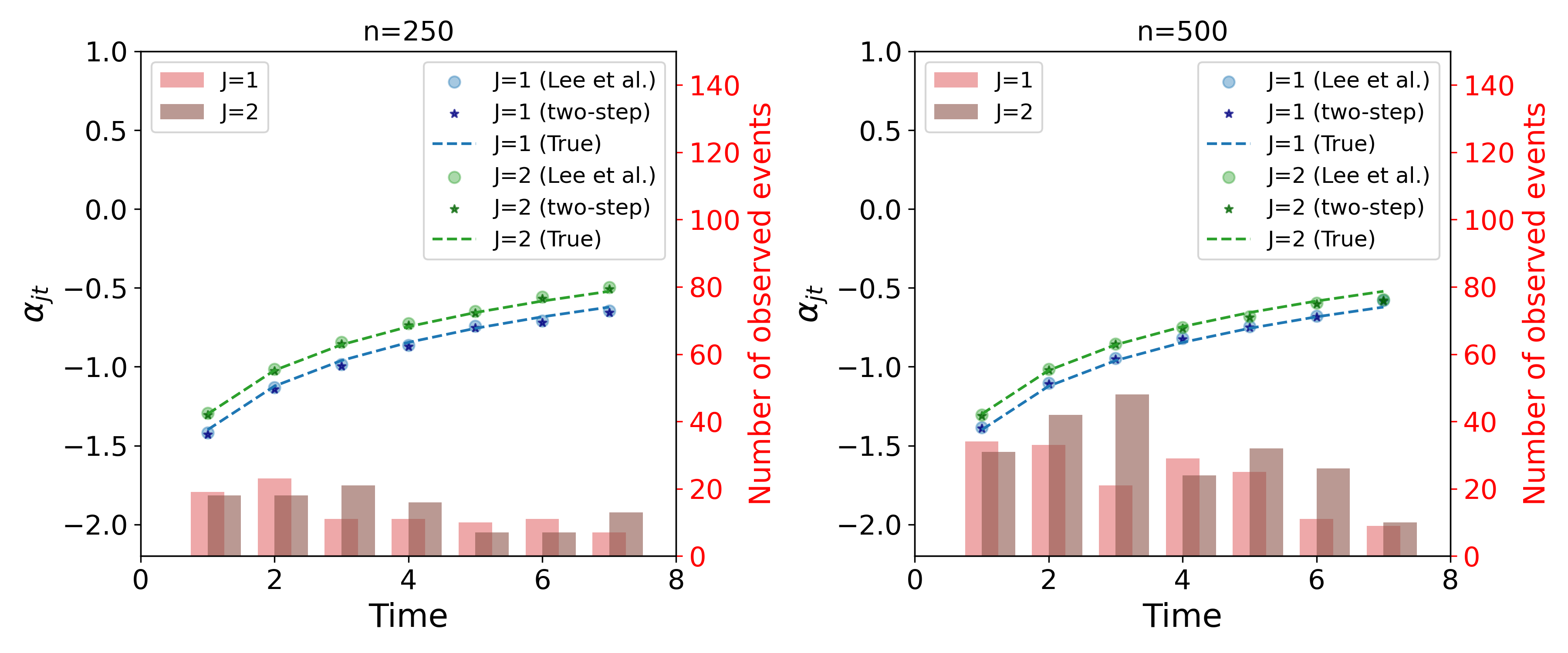
Figure S2 : Simulation results of small sample size. Results of ${\alpha}_{jt}$. Each panel is based on a different sample size. Number of observed events are shown in red and brown bars for event types $j=1$ and $j=2$, respectively. True values and mean of estimates are in blue and green for $j=1$ and $j=2$. True values are shown in dashed lines, mean of estimates based on Lee et al. and the proposed two-step approach denoted by circles and diamonds, respectively.

Appendix E. Simulation Results of Sure Independence Screening

Here we describe and demonstrate sure independent screening procedure (SIS) and SIS followed by lasso (SIS-L) of Fan et al. (2010) ¹⁶ and Saldana and Feng (2018) ¹⁸ applied within the proposed two-step approach.

To conduct SIS, we fit a marginal regression for each covariate individually using the first step of our proposed approach. The SIS procedure subsequently assesses the importance of features by ranking them according to the magnitude of their marginal regression coefficients. Then, the selected sets of variables are given by

$$\widehat{\mathcal{M}}_{j,w_{n}}=\{1\leq k\leq p\,:\,|\widehat{\beta}_{jk}|\geq w_{n}\}\,\,\,\,\,j=1,\ldots,M\,,$$

where $w_{n}$ is a threshold value. We adopt the data-driven threshold of ¹⁸. Specifically, given data of the form $\{X_{i},\delta_{i},J_{i},Z_{i}\,;\,i=1,\dots,n\}$, a random permutation $\pi$ of $\{1,\ldots,n\}$ is used to decouple $Z_{i}$ and $(X_{i},\delta_{i},J_{i})$ so that the resulting data $\{X_{i},\delta_{i},J_{i},Z_{\pi(i)}\,;\,i=1,\dots,n\}$ follow a model in which the covariates have no predicted power over the survival time of any event type. For the permuted data, we re-estimate individual regression coefficients and get $\widehat{\beta}^{*}_{jk}$, $k=1,\ldots,p$, $j=1,\dots,M$. The data-driven threshold used here is defined by

$$w_{n}=\max_{1\leq j\leq M,1\leq k\leq p}|\widehat{\beta}^{*}_{jk}|\,.$$

For SIS-L procedure, the lasso regularization is then added in the first step of our procedure applied to the set of covariates selected by SIS.

The simulated datasets (Setting 20–22) consist of $n=1,000$ observations and $p=15,000$ covariates. Each covariate is a zero-mean normally distributed with variance 1. Three settings were considered: with independent covariates ($\rho=0$), and with correlated covariates such that $Cov(Z_{il},Z_{ih})=\rho^{|l-h|}$ and $\rho=0.5,0.9$, following a similar approach as Zhao et al. (2012) ¹⁷. To ensure appropriate survival probabilities, covariates were truncated to be within $[-3,3]$. We considered $M=2$ competing events with $d=8$. The first five components of $\beta_{1}$ and $\beta_{2}$ were set to be non-zero, and the remaining coefficients set to zero. The non-zero parameters $\beta_{1k}$, $k=1,\ldots,5$, took on the values of $-0.7,-0.6,0.8,0.7,-0.8$ while $\beta_{2k}$, $k=1,\ldots,5$, had values of $0.7,0.8,-0.8,-0.6,-0.7$. Additionally, $\alpha_{1t}=-3.2+0.3\log t$ and $\alpha_{2t}=-3.3+0.4\log t$.

For SIS-L, the lasso parameters $\eta_{1}$ and $\eta_{2}$ were tuned using a grid search and 3-fold cross-validation, where $\log\eta_{1},\log\eta_{2}$ ranged between -12 to -2 with a step size of 0.5. The selected $\eta_{1},\eta_{2}$ maximize the global-AUC. The simulation results are summarised in Tables S4-S6.

The mean (SE) of the data-driven thresholds, $w_{n}$, of the SIS procedure were $0.224\;(0.015)$, $0.224\;(0.017)$, and $0.230\;(0.018)$, for $\rho$ values of 0, 0.5, and 0.9, respectively. The means and SEs of the selected regularization parameters of the SIS-L are shown in Table S4. The size of the selected models, the false positive (FP) and false negative (FN) are summarized in Table S5. As expected, higher values of $\rho$ result in higher number of FPs. Additionally, adding lasso regularization resulted in similar or reduced mean selected-model size and the mean FP. Both methods resulted with similar performance measures, as shown in Table S6. Adding lasso after the SIS, allowed us to retain a smaller set of covariates, while maintaining similar performances.

Table S4 : Simulation results of SIS-L using the first step of the proposed two-step approach. Results include the mean and standard error of the chosen regularization parameters $\log\eta_{1}$ and $\log\eta_{2}$.

$\rho$	0.0		0.5		0.9
	Mean	SE	Mean	SE	Mean	SE
$\eta_{1}$	-4.323	1.262	-5.735	1.120	-7.285	1.142
$\eta_{2}$	-4.505	1.711	-5.140	0.714	-6.540	1.002

Table S5 : Simulation results of SIS and SIS-L procedures using the first step of the proposed two-step approach. Results include mean and SE of the selected-model size (Size), false positive (FP), and false negative (FN).

		Size		$\mbox{FP}_{1}$		$\mbox{FN}_{1}$		Size		$\mbox{FP}_{2}$		$\mbox{FN}_{2}$
		Mean	SE	Mean	SE	Mean	SE	Mean	SE	Mean	SE	Mean	SE
	$\rho$
SIS	0.0	5.56	0.88	0.56	0.88	0.00	0.00	5.49	0.95	0.52	0.93	0.02	0.14
	0.5	5.50	1.50	0.78	1.33	0.28	0.51	6.56	1.05	1.67	0.96	0.11	0.31
	0.9	10.84	3.82	6.06	3.58	0.22	0.60	14.03	2.98	10.47	2.76	1.44	0.50
SIS-L	0.0	4.29	2.40	0.40	0.71	1.11	2.09	4.25	2.43	0.38	0.82	1.13	2.08
	0.5	5.48	1.51	0.76	1.33	0.28	0.51	5.69	1.09	0.80	0.99	0.11	0.31
	0.9	8.02	3.12	3.34	2.80	0.32	0.86	7.21	3.18	3.83	2.87	1.62	0.81

Table S6 : Simulation results of SIS and SIS-L procedures using the proposed two-step approach. Results include mean and SE of selected models metrics: AUC, BS, $\mbox{AUC}_{1}$, $\mbox{AUC}_{2}$, $\mbox{BS}_{1}$, and $\mbox{BS}_{1}$.

		AUC		BS		$\mbox{AUC}_{1}$		$\mbox{AUC}_{2}$		$\mbox{BS}_{1}$		$\mbox{BS}_{2}$
$\rho$		Mean	SE	Mean	SE	Mean	SE	Mean	SE	Mean	SE	Mean	SE
0.0	SIS	0.786	0.002	0.082	0.000	0.789	0.002	0.784	0.002	0.080	0.001	0.083	0.000
	SIS-L	0.789	0.002	0.084	0.000	0.792	0.002	0.786	0.001	0.083	0.001	0.085	0.000
0.5	SIS	0.774	0.001	0.082	0.001	0.755	0.001	0.793	0.003	0.081	0.000	0.082	0.001
	SIS-L	0.780	0.001	0.082	0.001	0.760	0.001	0.799	0.003	0.081	0.000	0.082	0.001
0.9	SIS	0.689	0.002	0.073	0.000	0.658	0.002	0.717	0.002	0.071	0.001	0.074	0.000
	SIS-L	0.708	0.002	0.073	0.000	0.673	0.002	0.740	0.002	0.071	0.001	0.073	0.000

Appendix F. MIMIC Data Analysis - Additional Discussion of the Results

The estimated coefficients for lab tests in the discharge-to-home ($j=1$) model were all negative, consistent with the expected result that abnormal test results at admission reduce the hazard of home discharge. Older age and recent admission were also found to reduce this hazard, while being married and having Medicare or “other” insurance increased it. Female gender, admission number, direct emergency admission, and night admission had a relatively small impact on this hazard. lasso regularization excluded several features from the model, including admissions number, night admission, direct emergency admission, ethnicity, Medicare insurance, single or widowed status, sex, and certain lab tests (Anion Gap, MCH, MCV, Magnesium, Phosphate, Platelet count, and Potassium).

The hazard of being discharged for further treatment ($j=2$) is primarily increased by admissions number, White ethnicity, Medicare insurance, single or widowed marital status, and older age. Direct emergency admission and being married decrease the hazard. Most lab test results had a minor impact on the hazard, except for white blood cell count, RDW, platelet count, glucose, creatinine, and bicarbonate, which reduced the hazard of being discharged for further treatment when abnormal. lasso regularization excluded only a few lab tests (Anion Gap, Chloride, MCHC, and MCV) and recent admission. The main factors that increased the hazard and were included in the model were admissions number, single or widowed marital status, Medicare insurance, and older age, while direct emergency admission, being married, and abnormal results of bicarbonate, creatinine, glucose, and platelet count decreased the hazard.

The hazard of in-hospital death ($j=3$) had the lowest number of observed events, resulting in noisier estimators, especially in later times. The lasso penalty had only a minor effect in terms of the number of excluded features. Lab test results that increased the hazard of in-hospital death were abnormal Anion Gap, Bicarbonate, Creatinine, Magnesium, White Blood Cells, RDW, and Sodium. Some of these lab test results had already been identified as predictors of in-hospital mortality in previous studies ³⁰, ³¹, ³², ³³. Other lab test results that increased the hazard of in-hospital death were abnormal Calcium total, Chloride, Glucose, Phosphate, Platelet Count, Potassium, Urea Nitrogen, and Red Blood Cells. Admissions number, “other” ethnicity, married status, recent admission, and older age also increased the hazard of in-hospital death. Direct emergency admission, black, Hispanic, or white ethnicity, and Medicare or “other” insurance types decreased the hazard of in-hospital death.

References

- Allison 1982 PD Allison. Discrete-time methods for the analysis of event histories. Sociological Methodology, 13:61–98, 1982. ISSN 00811750, 14679531. URL http://www.jstor.org/stable/270718.
- Lee et al. 2018 M Lee, EJ Feuer, and JP Fine. On the analysis of discrete time competing risks data. Biometrics, 74(4):1468–1481, 2018. ISSN 0006-341X, 1541-0420. doi: 10.1111/biom.12881.
- Wu et al. 2022 W Wu, K He, X Shi, DE Schaubel, and JD Kalbfleisch. Analysis of hospital readmissions with competing risks. Statistical Methods in Medical Research, 31(11):2189–2200, 2022. doi: 10.1177/09622802221115879.
- Kalbfleisch and Prentice 2011 JD Kalbfleisch and RL Prentice. The Statistical Analysis of Failure Time Data. Wiley, 2nd edition, 2011. ISBN 978-1-118-03123-0.
- Klein and Moeschberger 2003 JP Klein and ML Moeschberger. Survival Analysis. Springer, 2003. ISBN 978-0-387-95399-1.
- Lequertier et al. 2021 V Lequertier, T Wang, J Fondrevelle, V Augusto, and A Duclos. Hospital length of stay prediction methods: A systematic review. Medical Care, 59(10):929–938, 2021.
- Awad et al. 2017 A Awad, M Bader–El–Den, and J McNicholas. Patient length of stay and mortality prediction: A survey. Health Services Management Research, 30(2):105–120, May 2017. ISSN 0951-4848, 1758-1044. doi: 10.1177/0951484817696212.
- Adhikari et al. 2010 NKJ Adhikari, RA Fowler, S Bhagwanjee, and GD Rubenfeld. Critical care and the global burden of critical illness in adults. The Lancet, 376(9749):1339–1346, October 2010. ISSN 01406736. doi: 10.1016/S0140-6736(10)60446-1.
- Johnson et al. 2022 A Johnson, L Bulgarelli, T Pollard, S Horng, LA Celi, and R Mark. MIMIC-IV (version 2.0). PhysioNet, June 2022. doi: https://doi.org/10.13026/7vcr-e114.
- Goldberger et al. 2000 AL Goldberger, LAN Amaral, L Glass, JM Hausdorff, PC Ivanov, RG Mark, JE Mietus, GB Moody, CK Peng, and HE Stanley. PhysioBank, PhysioToolkit, and PhysioNet: Components of a New Research Resource for Complex Physiologic Signals. Circulation, 101(23), June 2000. ISSN 0009-7322, 1524-4539. doi: 10.1161/01.CIR.101.23.e215. URL https://www.ahajournals.org/doi/10.1161/01.CIR.101.23.e215.
- Tutz et al. 2016 G Tutz, M Schmid, et al. Modeling discrete time-to-event data. Springer, 2016.
- Möst et al. 2016 S Möst, W Pößnecker, and G Tutz. Variable selection for discrete competing risks models. Quality & Quantity, 50:1589–1610, 2016.
- Schmid and Berger 2021 M Schmid and M Berger. Competing risks analysis for discrete time-to-event data. Wiley Interdisciplinary Reviews: Computational Statistics, 13(5):e1529, 2021.
- Hastie et al. 2009 T Hastie, R Tibshirani, and JH Friedman. The elements of statistical learning: data mining, inference, and prediction. Springer, 2009.
- Fan and Lv 2008 J Fan and J Lv. Sure independence screening for ultrahigh dimensional feature space. Journal of the Royal Statistical Society: Series B (Statistical Methodology), 70(5):849–911, 2008. doi: 10.1111/j.1467-9868.2008.00674.x.
- Fan et al. 2010 J Fan, Y Feng, and Y Wu. High-dimensional variable selection for cox’s proportional hazards model. Institute of Mathematical Statistics, 2010.
- Zhao and Li 2012 SD Zhao and Y Li. Principled sure independence screening for cox models with ultra-high-dimensional covariates. Journal of multivariate analysis, 105(1):397–411, 2012.
- Saldana and Feng 2018 DF Saldana and Y Feng. Sis: An r package for sure independence screening in ultrahigh-dimensional statistical models. Journal of Statistical Software, 83(2):1–25, 2018.
- Meir et al. 2022 T Meir, R Gutman, and M Gorfine. Pydts: A python package for discrete-time survival (regularized) regression with competing risks. arXiv, 2022. doi: 10.48550/ARXIV.2204.05731. URL https://arxiv.org/abs/2204.05731.
- Cox 1972 DR Cox. Regression models and life-tables. Journal of the Royal Statistical Society: Series B (Methodological), 34(2):187–202, 1972. ISSN 00359246. doi: 10.1111/j.2517-6161.1972.tb00899.x.
- Cox 2018 DR Cox. Analysis of binary data. Routledge, 2018.
- Gail et al. 1981 MH Gail, JH Lubin, and LV Rubinstein. Likelihood calculations for matched case-control studies and survival studies with tied death times. Biometrika, (3):703–707, 1981.
- Fan et al. 2012 J Fan, Y Feng, and X Tong. A road to classification in high dimensional space: the regularized optimal affine discriminant. Journal of the Royal Statistical Society: Series B (Statistical Methodology), 74(4):745–771, 2012.
- Fan and Song 2010 J Fan and R Song. Sure independence screening in generalized linear models with np-dimensionality. The Annals of Statistics, 38(6):3567–3604, 2010.
- Fan et al. 2011 J Fan, Y Feng, and R Song. Nonparametric independence screening in sparse ultra-high-dimensional additive models. Journal of the American Statistical Association, 106(494):544–557, 2011.
- Yuan and Lin 2006 M Yuan and Y Lin. Model Selection and Estimation in Regression with Grouped Variables. Journal of the Royal Statistical Society. Series B (Statistical Methodology), 68(1):49–67, 2006. URL http://www.jstor.org/stable/3647556.
- Van der Vaart 2000 Aad W Van der Vaart. Asymptotic statistics. Cambridge university press, 2000.
- Heagerty and Zheng 2005 PJ Heagerty and Y Zheng. Survival model predictive accuracy and roc curves. Biometrics, 61(1):92–105, 2005.
- Blanche et al. 2015 P Blanche, C Proust-Lima, L Loubere, C Berr, JF Dartigues, and H Jacqmin-Gadda. Quantifying and comparing dynamic predictive accuracy of joint models for longitudinal marker and time-to-event in presence of censoring and competing risks. Biometrics, 71(1):102–113, 2015.
- Zhong et al. 2021 J Zhong, J Gao, JC Luo, JL Zheng, GW Tu, and Y Xue. Serum creatinine as a predictor of mortality in patients readmitted to the intensive care unit after cardiac surgery: a retrospective cohort study in China. Journal of Thoracic Disease, 13(3):1728–1736, March 2021. ISSN 20721439, 20776624. doi: 10.21037/jtd-20-3205. URL https://jtd.amegroups.com/article/view/49824/html.
- Wernly et al. 2018 B Wernly, M Lichtenauer, NAR Vellinga, EC Boerma, C Ince, M Kelm, and C Jung. Blood urea nitrogen (BUN) independently predicts mortality in critically ill patients admitted to ICU: A multicenter study. Clinical Hemorheology and Microcirculation, 69(1-2):123–131, May 2018. ISSN 13860291, 18758622. doi: 10.3233/CH-189111. URL https://www.medra.org/servlet/aliasResolver?alias=iospress&doi=10.3233/CH-189111.
- Meynaar et al. 2013 IA Meynaar, AH Knook, S Coolen, H Le, MM Bos, F Van Der Dijs, Marieke von Lindern, and EW Steyerberg. Red cell distribution width as predictor for mortality in critically ill patients. Neth J Med, 71(9):488–493, 2013.
- Bazick et al. 2011 HS Bazick, D Chang, K Mahadevappa, FK Gibbons, and KB Christopher. Red cell distribution width and all-cause mortality in critically ill patients*:. Critical Care Medicine, 39(8):1913–1921, August 2011. ISSN 0090-3493. doi: 10.1097/CCM.0b013e31821b85c6. URL http://journals.lww.com/00003246-201108000-00008.