Amplitude amplification-inspired QAOA: Improving the success probability for solving 3SAT

Abstract

The Boolean satisfiability problem (SAT), in particular 3SAT with its bounded clause size, is a well-studied problem since a wide range of decision problems can be reduced to it. Due to its high complexity, examining potentials of quantum algorithms for solving 3SAT more efficiently is an important topic. Since 3SAT can be formulated as unstructured search for satisfying variable assignments, the amplitude amplification algorithm can be applied. However, the high circuit complexity of amplitude amplification hinders its use on near-term quantum systems. On the other hand, the Quantum Approximate Optimization Algorithm (QAOA) is a promising candidate for solving 3SAT for Noisy Intermediate-Scale Quantum devices in the near future due to its simple quantum ansatz. However, although QAOA generally exhibits a high approximation ratio, there are 3SAT problem instances where its success probability decreases using current implementations. To address this problem, in this paper we introduce amplitude amplification-inspired variants of QAOA to improve the success probability for 3SAT. For this, (i) three amplitude amplification-inspired QAOA variants are introduced and implemented, (ii) the variants are experimental compared with a standard QAOA implementation, and (iii) the impact on the success probability and ansatz complexity is analyzed. The experiment results show that an improvement in the success probability can be achieved with only a moderate increase in circuit complexity.

Keywords: 3SAT, QAOA, amplitude amplification, Grover mixer, success probability

1 Introduction

The Boolean satisfiability problem (SAT) is a well-studied decision problem in computer science [1, 2, 3]. A range of application scenarios from formal verification of hardware [4] to planning problems [1, 5] can be encoded as SAT instances. Due to its strict form and its limitation of clause size to three literals, often 3SAT is considered, because all SAT instances can be reduced to 3SAT [6]. Various solvers for 3SAT exist on classical computers. However, since 3SAT is NP-complete [7], these solvers have high runtime complexity in the worst case, and therefore several works are currently investigating the possibility of quantum algorithms for solving 3SAT [8, 9].

Quantum computing promises to speed up various applications. To implement 3SAT solvers, different quantum algorithms, such as amplitude amplification [10, 11] or variational approaches such as the Quantum Approximate Optimization Algorithm (QAOA) [12], have been employed. However, current Noisy Intermediate-Scale Quantum (NISQ) devices are characterized by a limited number of qubits and a high rate of gate errors [13]. This restricts the circuit size of quantum algorithms executable on current quantum hardware. Although amplitude amplification is optimal in its complexity for general unstructured search problems [14], the quantum circuit that is required to solve 3SAT for larger instances exceeds the limits imposed by the current NISQ devices.

As variational quantum algorithms such as QAOA generally require shallower circuits, they have the potential to be used for 3SAT on NISQ devices. Although QAOA was originally proposed as an algorithm for the MAX-CUT problem [12], it uses a cost function that can be adapted to the specific problem at hand. Thus, QAOA is applied to a broad range of optimization problems [12, 15, 16, 17]. However, while in certain applications it was experimentally shown that QAOA obtains a set of solutions of robust approximation ratio [9], the optimization procedure tends to amplify suboptimal solutions [18]. Thus, the original implementation of QAOA might find wrong solutions for decision problems such as the 3SAT problem.

For general optimization problems, it has been experimentally demonstrated that the approximation ratio of QAOA can be improved by various adjustments to the algorithm. These include reformulations of the cost function [17, 19], the used mixing operator [16], or the parameter initialization strategy [20, 21, 22]. Some of these adaptions [16, 23] further make use of concepts introduced in amplitude amplification algorithms such as Grover’s search algorithm [24, 10, 25, 11] and variational adaptions thereof [8, 26]. Since 3SAT can also be formulated as unstructured search for satisfying assignments, adaptions that make use of concepts from amplitude amplification might improve the performance of QAOA for 3SAT as well. However, so far it has not been investigated whether an adapted QAOA algorithm can overcome the previously described problems of QAOA for solving 3SAT.

In this paper, we experimentally investigate if adapting QAOA using concepts from amplitude amplification improves the success probability for 3SAT (Section 6.1) and evaluate how such adaptions influence the computational complexity of the ansatz (Section 6.2). To this end, we implement three different variants of QAOA and compare them using randomly generated formulas.

The remainder of this paper is organized as follows: Section 2 gives the required background on the 3SAT problem and presents QAOA and amplitude amplification. Section 3 covers how QAOA can be applied to solve 3SAT and highlights shortcomings of the algorithm which serve as the motivation for the paper. Section 4 presents the three different adapted QAOA variants that are evaluated by the experiments described in Section 5. Section 6 highlights the results of the experiments and Section 7 summarizes related approaches and optimizations of QAOA. The results are discussed regarding their applicability in building 3SAT solvers on quantum computers in Section 8, before summarizing this work and presenting future research opportunities in Section 9.

2 Background

In this section, first the SAT and 3SAT problem are introduced. It is followed by a brief description of QAOA. Since the adaptions of QAOA presented in Section 4 make use of concepts of amplitude amplification, this algorithm is introduced at the end of this section.

2.1 Boolean satisfiability

As stated above, determining the satisfiability of Boolean formulas (SAT) is a well-studied problem since a wide range of decision problems can be reduced to instances of SAT. Especially the 3SAT variant of the problem is studied in the context of quantum algorithms due to its simple structure and convenient mapping to quantum circuits.

The 3SAT problem concerns propositional formulas $\phi=\bigwedge_{j=1}^{m}c_{j}$ in conjunctive normal form. These formulas are composed of $m$ clauses, each containing the disjunction of three literals: $c_{j}=\bigvee_{i=1}^{3}l_{i,j}$. Each literal $l_{i,j}$ is either an atomic variable $a_{k}$ from the set of Boolean variables $\{a_{1},\dots a_{n}\}$ or its negation $\lnot a_{k}$. The literals are referred to as negative if its atomic variable is negated and as positive otherwise. To define solutions for 3SAT formulas, the following definition is required:

Definition (3SAT interpretation).

An interpretation $v$ is a function that assigns $1$ or $0$ to 3SAT formulas according to the following rules:

• For an atom $a_{k}$: $v(a_{k})=0$ or $v(a_{k})=1$.

• For a literal $l_{i,j}$ containing the atom $a_{k}$: $v(l_{i,j})=v(a_{k})$ if the literal is positive and $v(l_{i,j})=1-v(a_{k})$ if the literal is negative.

• For a clause $c_{j}$: $v(c_{j})=1$ iff for one of its literals $v(l_{i,j})=1$ holds, and $v(c_{j})=0$ otherwise.

• For a 3SAT formula $\phi$: $v(\phi)=\prod_{j=1}^{m}v(c_{j})$.

An interpretation represents the evaluation of a formula to the truth values true and false. Since the assignment of truth values to atomic variables can be represented as a binary vector, we generally refer to an interpretation $v$ by its variable assignment $\vec{x}=(x_{1},\dots,x_{n})=(v(a_{1}),\dots,v(a_{n}))$. The evaluation of the formula according to this variable assignment is then denoted as

$$\phi(\vec{x})=\prod_{j=1}^{m}c_{j}(\vec{x})=1.$$ (1)

Using this evaluation, the 3SAT problem is given as:

Definition (3SAT problem).

The input is a 3SAT formula $\phi$. The goal is to decide whether there exists a variable assignment $\vec{x}$ such that $\phi(\vec{x})=1$. Such a satisfying interpretation is referred to as a model.

Although only the question of the satisfiability of given formulas is of interest for this decision problem, a satisfying variable assignment $\vec{x}$ can usually be obtained from 3SAT solvers for satisfiable instances.

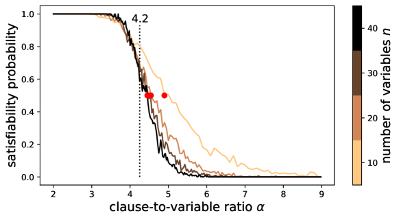
Figure 1: The proportion of satisfiable formulas for randomly generated 3SAT instances, which serves as an indication of the phase transition in the satisfiability probability. The points at each line mark the interpolated point where this proportion reaches $50\%$. As the number of variables $n$ increases, the points approach a clause-to-variable ratio of $\alpha^{\prime}\approx 4.2$ as indicated by the dotted line.

The 3SAT problem is one of the prime examples of NP-complete problems. Many studies were conducted to classify the computational resources required to solve instances of the 3SAT problem depending on specific properties of the input formulas [27, 2, 3]. One of these properties is the satisfiability probability. This is the probability that there exists a satisfying variable assignment for a random 3SAT formula. This satisfiability probability is closely linked to the clause-to-variable-ratio of randomly generated 3SAT formulas [27, 28]. Figure 1 shows the satisfiability probability for randomly generated formulas with a fixed number of variables $n$ and a varying clause-to-variable ratio $\alpha=m/n$. The figure shows that the satisfiability probability decreases sharply around a clause-to-variable ratio $\alpha^{\prime}\approx 4.2$ [28, 29, 30]. In this so-called phase transition region, problem instances change from formulas with a small number of clauses, which are satisfiable with high probability, to very constrained formulas that are almost certainly unsatisfiable. This change in satisfiability probability affects the runtime complexity of SAT solvers. For formulas near the phase transition, the time required to solve them generally increases. This phenomenon was experimentally shown by examining the computing time required for backtracking search-based solvers [27], the Davis-Putnam procedure [29], and similar algorithms [30]. Moreover, it has also been observed that the phase transition affects quantum algorithms for 3SAT. For formulas in the phase transition region, the probability that satisfying variable assignments are obtained decreases [9, 31]. Since the hardest instances for the 3SAT problem are concentrated near the phase transition region, this classification supports finding appropriate problem instances for testing and verifying newly devised 3SAT solving algorithms. As such, the clause-to-variable ratio is also used to classify the inputs for the experiments shown in Section 5.

A common characteristic to measure the quality of quantum algorithms solving 3SAT is the success probability for randomly generated formulas. It describes the probability that the decision (satisfiable or unsatisfiable) that is obtained by an algorithm for a formula of a specific clause-to-variable ratio is correct. This value will also be used in this work to inspect the performance of the proposed variants.

Another variant of the SAT problem is the MAX-3SAT problem, which formulates 3SAT as an optimization problem. This problem seeks to not specifically find a variable assignment $\vec{x}$ that satisfies the overall formula $\phi$, but it aims to give assignments that maximize the number of satisfied 3SAT clauses. These assignments can serve, for example, as heuristics for planning problems [5].

Using the notation from Equation 1, the goal of MAX-3SAT is to minimize the cost function

$$C_{\phi}(\vec{x})=\sum_{j=1}^{m}(1-c_{j}(\vec{x})),$$ (2)

which counts the number of unsatisfied clauses in a given formula containing $m$ clauses. In contrast to the success probability that is used to evaluate algorithms solving 3SAT, for optimization algorithms such as MAX-3SAT, the approximation ratio is evaluated. This is the ratio between the number of clauses that are satisfied by a variable assignment that is obtained from an optimization algorithm and the number of clauses that are satisfied in an optimal assignment. For a given 3SAT formula $\phi$, any optimal assignment for the MAX-3SAT problem satisfies $m_{opt}\leq m$ clauses. If $\phi$ is not satisfiable, $m_{opt}<m$ holds. For an arbitrary variable assignment $\vec{x}$ that satisfies $m_{\vec{x}}$ clauses, the approximation ratio is given as $m_{\vec{x}}/m_{opt}$. Currently, a lot of research in the field of quantum algorithms focuses on improving the approximation ratio for optimization problems such as MAX-3SAT using a quantum computer. One of the algorithms that are applied to achieve this goal is QAOA.

2.2 The Quantum Approximate Optimization Algorithm

The Quantum Approximate Optimization Algorithm (QAOA) is a variational quantum algorithm designed to solve combinatorial optimization problems and was first proposed as a quantum solution for the MAX-CUT problem [12]. This algorithm uses an ansatz that is modeled for the specific problem at hand. This allows it to also be extended to other problems, including some commonly known NP-complete problems [32].

At its core, QAOA aims to find the states with minimal eigenvalue of a given Hamiltonian $H_{C}$, which encodes the cost function $C:\{0,1\}^{n}\rightarrow\mathbb{R}$ associated with a combinatorial optimization problem. For a solution candidate given by the binary vector $\vec{x}\in\{0,1\}^{n}$, $H_{C}$ encodes the cost of this solution in its eigenvalues as

$$H_{C}\ket{\vec{x}}=C(\vec{x})\ket{\vec{x}}.$$ (3)

Therefore, the eigenvalues are minimal for optimal solutions with respect to $C(\vec{x})$. The ansatz consists of a circuit preparing an initial state, followed by $p$ repetitions that alternately apply the phase-separation operator $U(H_{C},\gamma_{i})=e^{-i\gamma_{i}H_{C}}$ and the mixer circuit $U(H_{B},\beta_{i})=e^{-i\beta_{i}H_{B}}$. The phase-separation circuit introduces a not-measurable phase that encodes the cost of the solutions. The mixer circuit is used to translate this phase into an adjustment of the measurement probability of the solution candidates. The unitary operations $U(H_{C},\gamma_{i})$ and $U(H_{B},\beta_{i})$ are parametrized by the real-valued vectors $\vec{\gamma}=(\gamma_{1},\dots,\gamma_{p})$ and $\vec{\beta}=(\beta_{1},\dots,\beta_{p})$. Applying this procedure to the initial state $\ket{+}^{\otimes n}$ takes the quantum system to the parametrized state

$$\ket{\vec{\gamma},\vec{\beta}}=\left(\prod_{i=1}^{p}U(H_{B},\beta_{i})U(H_{C},\gamma_{i})\right)\ket{+}^{\otimes n},$$ (4)

with the mixer Hamiltonian given as $H_{B}=\sum_{i=1}^{n}X_{i}$, which is often referred to as the transverse-field mixer [19].

By executing the described quantum circuit, a set of binary vectors representing solution candidates to the optimization problem is sampled and their average cost is calculated. In the variational loop, a classical optimizer is used to find optimal parameters $\vec{\gamma}^{*},\vec{\beta}^{*}$ such that the expected cost of the measured solutions is minimized. In other words, the algorithm computes

$$\min_{\vec{\gamma},\vec{\beta}}\braket{\vec{\gamma},\vec{\beta}}{H_{C}}{\vec{\gamma},\vec{\beta}}.$$ (5)

Using the optimal parameters $\vec{\gamma}^{*},\vec{\beta}^{*}$ that are found by the classical optimizer, a set of solutions that approximately minimizes the problem cost function $C(\vec{x})$ can be measured. Assuming that the number of repetitions $p$ of $U(H_{B},\beta_{i})$ and $U(H_{C},\gamma_{i})$, is sufficiently large, such a set of solutions should be found [12]. However, giving estimates for the required $p$ is still an actively studied question. This value is also referred to as the QAOA depth of the ansatz as it directly influences the circuit depth of the executed quantum circuit.

2.3 Amplitude amplification

Grover’s algorithm [11], the first algorithm making use of the concept of amplitude amplification, performs unstructured search for a unique solution state identified by an oracle on a quantum computer. It speeds up this process relative to classical unstructured search by requiring $O(\sqrt{N})$ evaluations of the oracle as opposed to $O(N)$ on a classical computer for a search space containing $N$ elements [11]. It further was shown that this algorithm is optimal in its runtime complexity up to a constant factor for unstructured search problems [14]. The idea behind this process is generalized to problems with multiple solution states in the amplitude amplification algorithm [10].

Similar to the phase-separation operator in QAOA, amplitude amplification requires an oracle that manipulates the phase of a state based on its membership in the set of solutions. Given some Boolean indicator function $f:\{0,1\}^{n}\to\{0,1\}$, the Grover oracle, sometimes referred to as the phase-flip oracle, maps each candidate state $\ket{\vec{x}}$ to $(-1)^{f(\vec{x})}\ket{\vec{x}}$. To translate this change in phase into a measurable amplification of the amplitude of a solution state, the Grover diffusion operator $2\ket{+}\bra{+}^{\otimes n}-I^{\otimes n}$ is used [33]. This process is repeatedly applied to the starting state $\ket{+}^{\otimes n}$, which represents the superposition of all solution candidates in an unconstrained search space. Depending on the size of the set of solutions and the size of the search space, a fixed limit can be specified for the number of applications of the oracle and the diffusion operator before the desired solution states are measured with certainty [33, 10].

Solution candidates for problems in NP, such as 3SAT, can be verified in polynomial time classically and therefore can also be verified using a polynomial-size quantum circuit [33]. Thus, a general unstructured search algorithm such as amplitude amplification is predestined to solve satisfiability problems. For the 3SAT problem, a solution candidate is a variable assignment represented by a bitstring $\vec{x}\in\{0,1\}^{n}$. The purpose of the phase oracle is then to mark assignments in the superposition of variable assignments if and only if they satisfy a given formula.

3 Motivation and Research Questions

The drawback of amplitude amplification algorithms for current NISQ devices is its requirement for deep quantum circuits. Due to QAOA’s shallower quantum circuits, the potential of applying QAOA to the 3SAT problem is actively studied. However, since QAOA is an optimization algorithm, currently only the optimization variant of 3SAT called MAX-3SAT, is considered [8, 9]. For applying QAOA to MAX-3SAT, the cost function in Equation (2) is encoded in a cost Hamiltonian $H_{\phi}$. There are various formulations of this Hamiltonian [32, 34, 35, 36, 37], with some focusing on reducing the number of operations required when implementing this cost function in the phase-separation operator. The formulations generally describe the cost Hamiltonian as a sum of clause operators

$$H_{\phi}=\sum_{j=1}^{m}H_{C_{j}}.$$ (6)

Each $H_{C_{j}}$ increases the eigenvalue of the variable assignments that do not satisfy the $j$-th clause. These clause operators are expressed as

$$H_{C_{j}}=\frac{1}{8}\prod_{i=1}^{3}(I+p_{i,j}Z_{a_{i,j}}).$$ (7)

In this equation, $p_{i,j}$ describes the polarity of the literal $l_{i,j}$ in the $j$-th clause with $p_{i,j}=1$ for positive literals and $p_{i,j}=-1$ for negative literals. Furthermore, the expression $Z_{a_{i,j}}$ describes that the Pauli operator $Z$ is applied to the qubit representing the atom of literal $l_{i,j}$. Depending on the polarity of the literal $l_{i,j}$, the individual factors in Equation (7) have eigenvalue $0$ if the literal is satisfied by the variable assignment. The factors have eigenvalue $2$ if the literal is not satisfied. Thus, if at least one literal in the disjunction is satisfied, the clause operator $H_{C_{j}}$ has eigenvalue $0$ for this variable assignment. By using QAOA to find the states with minimal eigenvalue for the cost Hamiltonian $H_{\phi}$, the algorithm will therefore find variable assignments that have eigenvalue $0$ for as many clause operators $H_{C_{j}}$ as possible. Thus, this variable assignment maximizes the number of satisfied clauses, which solves the MAX-3SAT problem. For details on how this cost operator is implemented as a quantum circuit see A.

To extend this algorithm for MAX-3SAT to solve the decision problem 3SAT, recent works focus on using the variable assignments that are obtained for MAX-3SAT and inferring whether they satisfy the given input [9, 8]. This is achieved by evaluating the formula classically using the sampled solutions.

Using experimental evaluations, it was found that QAOA exhibits a good approximation ratio for MAX-3SAT [9]. However, by reasoning from the approximated solution of the MAX-3SAT problem, incorrect solutions are often obtained for the 3SAT decision problem. Considering a satisfiable 3SAT formula in conjunctive normal form, a measured variable assignment satisfying 99% of the given clauses would be a respectable result for an algorithm approximating the MAX-3SAT problem. However, this would be evaluated to the wrong result of unsatifiable for the decision problem variant. Similar observations were made by Bennett and Wang [18]. In their work, they found that the Quantum Walk Optimization Algorithm (QWOA), a generalization of QAOA, tends to amplify suboptimal solutions to increase the approximation ratio as they are more numerous than optimal solutions. Thus, the standard QAOA implementation leaves room for improvement when applied to 3SAT.

Therefore, the objective of this work is to exploit the advantages of amplitude amplification to improve the success probability of the QAOA for 3SAT. Thus, we formulate the following research questions:

• RQ1: Can mechanisms found in amplitude amplification be used to improve the success probability of QAOA for the 3SAT problem?

• RQ2: How does adapting the QAOA ansatz using concepts from amplitude amplification influence the computational complexity of the ansatz?

4 Amplitude amplification-inspired QAOA variants

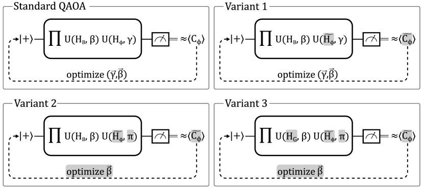
Figure 2: A schematic overview of the three different variants of QAOA implemented in this work and the standard QAOA implementation for MAX-3SAT. The adaptions applied to the standard QAOA implementation for the MAX-3SAT problem are highlighted.

To answer the research questions, we examine and experimentally compare three different variants of QAOA that make use of ideas employed in amplitude amplification to improve the success probability for the 3SAT problem. We present the adaptions as a gradual reformulation of QAOA until it almost matches the amplitude amplification algorithm. Figure 2 gives an overview of standard QAOA and the proposed adaptions we implement for the experiments in Section 5:

• Variant 1: An adaption of QAOA that optimizes using a binary cost function.

• Variant 2: An extension of Variant 1, where the parameters $\vec{\gamma}$ are fixed to $\gamma_{i}=\pi$. The classical optimization step will only optimize the mixer parameters $\vec{\beta}$.

• Variant 3: An extension of Variant 2, that employs the Grover mixer.

In the following, these variants of QAOA are explained in detail.

4.1 Variant 1: Cost function and phase-separation operator

Variant 1 applies an adapted binary cost function. To guide the approximation algorithm away from amplifying suboptimal solutions, this function penalizes all but optimal solutions equally. Given some 3SAT formula $\phi$, this objective function $\widetilde{C_{\phi}}(\vec{x})$ is given as

$$\widetilde{C_{\phi}}(\vec{x})=\cases{0&if $\phi(\vec{x})=1$\\ 1&if $\phi(\vec{x})=0$\\ },$$ (8)

where $\phi(\vec{x})=1$ represents that the formula $\phi$ evaluates to true given the variable assignment $\vec{x}$ and $\phi(\vec{x})=0$ representes that the formula evaluates to false. Similarly, the corresponding cost Hamiltonian $\widetilde{H_{\phi}}$ has eigenvalue $1$ for quantum states $\ket{\vec{x}}$ representing unsatisfying assignments and eigenvalue $0$ for satisfying assignments. The expected cost $\braket{\vec{\gamma},\vec{\beta}}{\widetilde{H_{\phi}}}{\vec{\gamma},\vec{\beta}}$ approximated by QAOA using this operator can therefore be seen as the proportion of unsatisfying assignments that are measured at the end of the circuit.

We implement the phase-separation operator for QAOA based on this cost function by reusing existing techniques for oracle synthesis [38]. We first present the general approach that is used to extend a bit-flip oracle to a phase-separation operator as it is used for our experiments. A general bit-flip oracle for a given function $f:\{0,1\}^{n}\to\{0,1\}$ is defined as

$$U\ket{\vec{x},y}=\ket{\vec{x},y\oplus f(\vec{x})}.$$ (9)

Thus, it encodes the result $f(\vec{x})$ by negating an ancilla qubit. This qubit can further be used to manipulate the phase of the examined quantum state as it is required in QAOA.

We perform this extension by noting that the required phase-separation operator $U(H_{C},\gamma)$ takes $\ket{\vec{x}}$ to $e^{-i\gamma C(\vec{x})}\ket{\vec{x}}$ for a given assignment of combinatorial variables $\vec{x}$ and an arbitrary objective function. Assuming the cost function is binary and given as $C(\vec{x})\in\{0,1\}$, this exact operation can also be performed using a bit-flip oracle, by applying the phase gate $P(-\gamma)$ before uncomputing:

$$\eqalign{\ket{\vec{x},0\oplus C(\vec{x})}&=\ket{\vec{x},C(\vec{x})}\\ &\binrel@{\longrightarrow}\binrel@@{\mathop{\kern 0.0pt\longrightarrow}\limits^{P(-\gamma)}}e^{-i\gamma C(\vec{x})}\ket{\vec{x},C(\vec{x})}\\ &\binrel@{\longrightarrow}\binrel@@{\mathop{\kern 0.0pt\longrightarrow}\limits^{U^{\dagger}}}e^{-i\gamma C(\vec{x})}\ket{\vec{x},0}.}$$ (10)

For the 3SAT problem, the cost function $\widetilde{C_{\phi}}(\vec{x})$ in Equation (8) is binary. We therefore perform the process in Equation (10) using an oracle circuit that flips the ancilla qubit if the given formula is satisfied. To obtain a phase-separation operator that matches $U(\widetilde{H_{\phi}},\gamma)$ and only introduces the phase if the formula is not satisfied, the ancilla qubit is negated before the oracle is applied.

4.2 Variant 2: Phase-flip oracle

With the adaption of Variant 1, first parts of amplitude amplification were incorporated into QAOA: The phase-separation operator based on a bit-flip oracle as presented above can be seen as a phase-flip oracle with an additional degree of freedom represented by the parameter $\gamma$. By fixing $\gamma=\pi$, the phase-flip oracle is obtained since $e^{-i\pi C(\vec{x})}\ket{\vec{x}}=(-1)^{C(\vec{x})}\ket{\vec{x}}$. Additionally, fixing this parameter simplifies the optimization loop, since then only the optimization over the mixer parameters $\vec{\beta}$ remains. We therefore evaluate the variant with the parameter $\gamma$ fixed to $\gamma=\pi$ as Variant 2 in our experiments.

4.3 Variant 3: Mixer and Grover diffusion

Similar to QAOA, amplitude amplification can be described as the repeated application of a gate that encodes a cost function (the phase-flip oracle) and a mixing gate (in the context of amplitude amplification referred to as the diffusion operator). The similarity between the phase-flip oracle and QAOA’s phase-separation operator has already been sketched in Section 4.2. In Variant 3, we further adapt QAOA by using the Grover mixer (GM-QAOA [16]), which closely resembles the diffusion operator in amplitude amplification.

Instead of the usual mixing Hamiltonian as presented in Section 2.2, the general Grover mixer uses the Hamiltonian $H_{F}=\ket{F}\bra{F}$, where $F$ is a set of feasible solution states and $\ket{F}$ is the equally weighted superposition of these states [16]. Since for 3SAT, the objective function decides whether a solution is feasible, the set $F$ is assumed to be all possible $n$ qubit binary strings representing assignments of $n$ Boolean variables. This implies $\ket{F}=\ket{+}^{\otimes n}$ and results in the mixing Hamiltonian $H_{G}=\ket{+}\bra{+}^{\otimes n}$.

By applying the reformulation of the resulting mixing unitary as presented in [16], it is possible to show how this gate can be implemented as a quantum circuit. In the following equations, we omit the register size $n$ to aid readability. Using the infinite sum for the matrix exponential, the mixing unitary is reformulated as

$$U(H_{G},\beta) =e^{-i\beta\ket{+}\bra{+}}$$ (11a)

$$=\sum_{k=0}^{\infty}\frac{1}{k!}(-i\beta)^{k}\left(\ket{+}\bra{+}\right)^{k}.$$ (11b)

For $k=0$, the matrix on the right-hand side reduces to $\left(\ket{+}\bra{+}\right)^{0}=I$. Furthermore since $\left(\ket{+}\bra{+}\right)^{2}=\ket{+}\braket{+}{+}\bra{+}=\ket{+}\bra{+}$, this matrix is idempotent. Therefore, $\left(\ket{+}\bra{+}\right)^{k}=\ket{+}\bra{+}$ is used for $k>1$ in Equation (11b) to give

$$U(H_{G},\beta) =I+\sum_{k=1}^{\infty}\frac{1}{k!}(-i\beta)^{k}\ket{+}\bra{+}$$ (11la)

$$=I+\left(e^{-i\beta}-1\right)\ket{+}\bra{+}$$ (11lb)

$$=H\left(I+\left(e^{-i\beta}-1\right)\ket{0}\bra{0}\right)H$$ (11lc)

$$=HX\left(I+\left(e^{-i\beta}-1\right)\ket{1}\bra{1}\right)XH$$ (11ld)

$$=HX\;\mathit{CP}_{n}(-\beta)\;XH,$$ (11le)

Figure 3: The quantum circuit for the Grover mixer [16] with the mixing Hamiltonian $H_{G}=\ket{+}\bra{+}^{\otimes n}$.

where $\mathit{CP}_{n}(-\beta)$ is the phase-shift gate on the $n$th qubit, which is controlled by the other $n-1$ qubits. Therefore, the Grover mixer can be built using two layers of Hadamard and $X$ gates and a controlled phase shift gate, resulting in the quantum circuit in Figure 3. Equation (11lb) further highlights the relationship between the Grover mixer and the diffusion operator. It shows that by setting $\beta=\pi$, the Grover mixer is equal to the diffusion operator $2\ket{+}\bra{+}-I$ up to a global phase, which gives the justification for its name.

5 Experiment setup

To answer RQ1, we implement the presented variants of QAOA using Qiskit and evaluate their success probability when solving 3SAT. For this evaluation, we use Qiskit’s simulator to obtain noise-free results. This section describes both the inputs for these experiments and the evaluation of the results in detail. We further implement and execute this experiment for an unmodified 3SAT solver based on QAOA for the MAX-3SAT problem as described in Section 3 as a baseline. To further evaluate how the QAOA depth influences the success probability of each variant, all experiments are executed for $p\in\{2,4,6,8,10\}$. For each variant and each selected QAOA depth, a set of 3SAT formulas is generated and the proportion of successful executions of the variants on these inputs is computed. There is a tradeoff between the used instance sizes and the computation time that is required for the simulation. We therefore keep the number of variables at $n=10$. To be able to study the effect of the 3SAT phase transition on the success probability, we evaluate formulas of clause-to-variable ratio $1.5\leq\alpha\leq 8$. This way, formulas on both sides of the phase transition region at $\alpha\approx 4.2$ are included. Thus, for each number of clauses $m$ between $m=15$ and $m=80$, $400$ 3SAT instances are evaluated by executing the process shown in Figure 4.

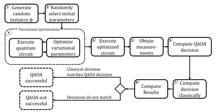
Figure 4: Experiment setup to approximate success probability. This experiment is executed for Variant 1-3 as well as the baseline implementation.

In Step 1 of the experiment, a 3SAT formula is randomly generated. Its clauses are composed by picking three of the $n=10$ available atomic variables with repetition. The variables are added to the overall disjunction as positive or negative literals with equal probability. In Step 2 and Step 3, the quantum algorithm is executed. The parameters are initialized and then optimized in the variational loop. As the classical optimizer for this experiment, we choose the implementation of the linear approximation-based optimizer COBYLA, provided in SciPy [39]. This optimizer was found to be preferable in low-noise scenarios [40], which is preferrable since we simulate the quantum circuits without noise.

For Variant 1-3, the variational loop finds values for the parameters $\vec{\gamma}^{*}$ and $\vec{\beta}^{*}$ (or only $\vec{\beta}^{*}$ for Variant 2 and Variant 3 respectively) that minimize the expected value of the cost function $\widetilde{C_{\phi}}(\vec{x})$ from Equation (8). For the baseline implementation, Step 3 minimizes $C_{\phi}(\vec{x})$ from Equation (2). The ansatz is then executed again using these optimized parameters in Step 4 to measure a set of variable assignments in Step 5. From these measurements, the decision (satisfiable or unsatisfiable) for the 3SAT problem instance is obtained in Step 6. The input formula is deemed satisfiable if and only if

$$\braket{\vec{\gamma}^{*},\vec{\beta}^{*}}{\widetilde{H_{\phi}}}{\vec{\gamma}^{*},\vec{\beta}^{*}}<1.$$ (11lm)

In other words, if the measurement using the optimal parameters produces at least one satisfying assignment, the formula is satisfiable. It decides the contrary if no such solution is found. Finally, in Step 7 the exact decision for the given input is calculated classically. We use the classical solver PySAT [41] for this purpose. Based on this result, one execution of the algorithm is deemed successful in Step 8 if the decision of the studied variant matches the decision obtained by the classical 3SAT solver.

The presented variants of QAOA employ rather computationally expensive oracles and mixers. The number of operations in the quantum circuits is too large to be executed on current devices for $n=10$. Thus, we perform the experiments using Qiskit’s built-in simulation capabilities. For simplicity, we use the classical function compiler in Qiskit, which makes use of tweedledum [38] to obtain the required bit-flip oracles for Variant 1-3. To obtain the measurements for the baseline implementation we use Qiskit’s built-in QAOA implementation [42]. Although the baseline implementation optimizes with respect to the function $C_{\phi}$, the final decision in Step 6 is still computed using $\widetilde{C_{\phi}}$ as for Variant 1-3. This allows us to compare the results using the same metric although different operators are optimized.

To further investigate the influence of the used optimizer on the success probability, we extend this evaluation by comparing different optimization procedures. We compare the optimizer that is used in this work (COBYLA) to different optimizers that are used in related works concerning variational quantum algorithms [9, 43, 44]: the limited memory BFGS method [45] and the Simultaneous Perturbation Stochastic Approximation (SPSA) algorithm [46]. For this comparison, we investigate the success probability of the baseline implementation and Variant 1-3 using formulas of clause-to-variable ratio $\alpha=4.5$. This value is chosen since our initial experiments found that formulas of this clause-to-variable ratio experience the lowest success probability for $n=10$. Lastly, the initial set of parameters that are chosen for the optimization (see Step 2) might influence the success probability of the inspected variants. Therefore, we also investigate the case where the optimization procedure is repeated five times with different sets of initial parameters and the result with the lowest cost is selected.

6 Experiment results

The results of the conducted experiments were analyzed in order to answer the research questions of this paper. The experiments have shown that the adaptions of QAOA presented in this paper influence the success probability positively (RQ1), but also increase the complexity of the quantum circuits (RQ2). The results are presented in detail below.

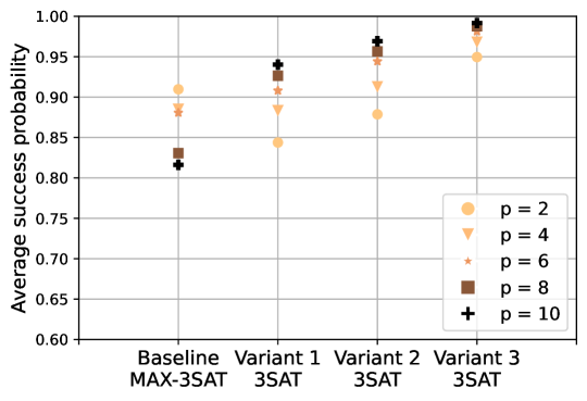
Figure 5: The success probability of the examined 3SAT solver variants for the examined QAOA depths $p$, over the range $[1.5,8.0]$ of clause-to-variable ratios.

6.1 Effect on the success probability

We first present the success probability of the different QAOA variants in our experiments. The implementations used for these experiments and the obtained experimental data are available online.

6.1.1 Comparison of QAOA variants

Figure 5 shows the average success probability of Variant 1-3 as well as the baseline implementation. These numbers were obtained by computing the proportion of successful executions of the process in Figure 4 over the whole range $[1.5,8.0]$ of examined clause-to-variable ratios. Figure 5 shows that the rewrite of the cost function to encode the decision problem in the phase-separation operator (Variant 1) alone only slightly improves the success probability for 3SAT when higher depth ansätze of $p=8$ and $p=10$ are used. Our experiments even suggest that the variational optimization of the parameters $\vec{\gamma}$ is not necessary: Variant 2 exhibits a higher success probability for p=8 and p=10 than both, Variant 1 and the baseline implementation. Finally, the introduction of the Grover mixer in Variant 3 has the most noticeable positive effect on the success probability as it improves the success probability to at least $0.94$ even for the smallest studied depth $p=2$.

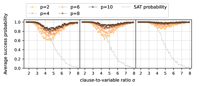
(a) Variant 1

(b) Variant 2

(c) Variant 3

Figure 6: The success probability for the examined variants for $n=10$ variables. The probability is shown for differing clause-to-variable ratio $\alpha$ and various depths $p$.

To highlight the dependence of the results on the satisfiability probability and its phase transition, Figure 6 shows the obtained success probability of the presented variants for each examined clause-to-variable ratio of the inputs. The satisfiability probability of these inputs is computed classically and is shown as a dotted line in each subplot. For all variants, the plot shows that the hardest instances for QAOA concentrate near the phase transition region. The success probability decreases for problem instances between $\alpha=4$ and $\alpha=5$. However, Figure 6(c) shows that Variant 3 is the least affected by this phenomenon. Even for the hardest instances in the phase transition region, the success probability only decreases to $0.8$ for the shallowest circuits of QAOA depth $p=2$.

6.1.2 Comparison of optimizers

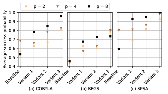
Figure 7: The success probability for the examined variants for the optimizers COBYLA, BFGS and SPSA and for different QAOA depths $p$ and 3SAT formulas with $\alpha=4.5$.

The improvement obtained by Variant 2 suggests that the optimization procedure is a limiting factor in the performance of the algorithm. Because Variant 2 omits half of the variational parameters by using the phase-flip oracle from amplitude amplification, it overcomes this limitation to some extent. Using the ansatz from Variant 2, the optimizer needs to optimize a smaller set of parameters, which improves the success probability.

We further evaluate the possible dependence of these findings on the optimization procedure by comparing different optimizers. Figure 7 shows the average success probability for the COBYLA, BFGS, and SPSA optimizers for formulas with clause-to-variable ratio $\alpha=4.5$. Figure 7 and Figure 7 show that the findings also hold up for different optimizers: For $p>2$, the success probability for Variant 1-3 is higher than that of the baseline implementation. Furthermore, Figure 7 shows that SPSA obtains a higher success probability than both COBYLA and BFGS for this experiment.

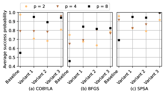
Figure 8: The success probability for the examined variants 3SAT formulas with $\alpha=4.5$ when using five random initial points for optimization and selecting the best result.

Lastly, Figure 8 compares the success probability of the different variants and of the baseline implementation when the optimization loop is repeated with different sets of randomly generated initial parameters. The baseline implementation even outperforms the examined variants for $p=2$ and the COBYLA optimizer (see Figure 8). However, already for $p=4$, its success probability decreases. This suggests that the ansatz that is used in the baseline implementation is expressible enough such that 3SAT can be solved with high success probability. However, the chance of finding parameters that minimize the cost function for the baseline implementation depends on the initial set of parameters. With five repetitions, as it is done in Figure 8, the chance to choose initial parameters that simplify the optimization step increases.

Although the success probability for Variant 1-3 also increases when multiple optimization rounds are used (Figure 8), the success probability for Variant 1-3 is less affected by the initial set of parameters. It is already greater than $0.75$ for the COBYLA optimizer and $p=8$ even with only a single round of optimization (Figure 7).

6.2 Effect on ansatz complexity

Although the examined changes to QAOA improve the success probability for the 3SAT problem, some of these adaptions come with an increase in circuit complexity. Compared to the used bit-flip oracles for the 3SAT problem in Variant 1-3, the phase-separation operator required for the baseline MAX-3SAT ansatz can be constructed with linear depth using rotations with at most three-qubit interactions (see A for details).

The most straightforward approach to obtaining a bit-flip oracle for the 3SAT problem is by using ancilla qubits to store the evaluation result of each clause. This result is obtained using single qubit negation and controlled negation gates using three control qubits. The result for the overall formula is then obtained using another CNOT gate that is controlled by all $m$ ancilla qubits. Nielsen and Chuang [33] show how such a gate can generally be constructed using a linear number of Toffoli gates and ancilla qubits. There further are implementations of this controlled negation that, although they use more operations in total, require no ancilla qubits and have the same asymptotic complexity [47]. Furthermore, there are more sophisticated approaches to constructing the bit-flip oracle for satisfiability problems [48, 49, 50], yet they still require a nonconstant number of ancilla qubits. Lastly, also the Grover mixer used in Variant 3 increases the ansatz complexity compared to the transverse-field mixer $H_{B}$. However, Equation (11le) shows that this increase in complexity is not as costly as for the cost operator: Apart from a phase gate controlled by $n-1$ qubits with linear depth, only two layers each of $H$ and $X$ gates have to be used.

To summarize, the adapted mixer in Variant 3 uses a linear amount of gates as opposed to the constant number of gates in Variant 1 and Variant 2. The asymptotic complexity of the ansatz circuit is dominated by the phase-separation operator with linear depth. Therefore, the asymptotic complexity of the overall ansatz circuit does not increase when compared to the implementation of QAOA for the MAX-3SAT problem. But since the examined circuits are small for the studied instances, this still amounts to a considerable increase of gate operations. Therefore, although the results show that the success probability can be improved, this improvement comes with the tradeoff of increased circuit complexity. However, the experiments suggest that the presented variants still are useful adaptions. Especially Variant 1 and Variant 2 increase the success probability using only the relatively cheap adaption for the phase-separation operator.

7 Related Work

The performance of the baseline implementation of QAOA for MAX-3SAT, when applied to the 3SAT problem, was extensively studied by Zhang et al. [9]. Their examination shows that the phase transition in the satisfiability probability impacts the success probability for the MAX-3SAT problem among other related problems. Their implementation contrasts the experiments performed in this paper since they make use of an incremental initialization strategy for the variational parameters and select the best result after multiple executions of the optimizer.

The modified phase-separation operator in Variant 1 has also been employed in a similar way by Jiang et al. [19]. They also use a cost Hamiltonian that solely distinguishes satisfying states from unsatisfying states. In contrast to our work, they use it to solve a problem more closely related to Grover’s original formulation, where there is only one possible solution state that should be amplified. Furthermore, they make use of the transverse-field mixer and fix its parameter $\beta$ to $\pi$.

To tackle the problem of variational quantum algorithms amplifying suboptimal solutions, Bennett and Wang [18] employ a similar adaption to Variant 1 to the more general framework of the Quantum Walk Optimisation Algorithm (QWOA). They present the Maximum Amplification Optimization Algorithm (MAOA) and apply it to combinatorial optimization problems. They use a similar distinction between good and bad solutions to classify the elements in the set of feasible solutions into ones meeting a certain threshold for the cost function and those that do not. They further show that the variational optimization process can be eliminated as the maximal amplification of the solutions state is obtained by a known set of parameters.

In Variant 3, the Grover mixer is introduced, which closely follows the diffusion operator used in amplitude amplification. This operation is essential to the variational reformulation of the Grover search algorithm [26, 8] and is further used in [16], who study the application of QAOA using this mixer on a range of optimization problems. They, however, focus on using this mixer on constrained optimization problems, where the set of feasible states is only a subset of the set of all possible states that are examined in our experiments.

Another approach that is closely related to Variant 3 is Threshold QAOA (Th-QAOA) [17]. Herein, the objective function is replaced by a similar operator based on a threshold. It is applied to optimization problems and distinguishes states with a cost larger than the given threshold from states with less or equal cost. They further combine this phase-separation operator with the Grover mixer [16] (GM-Th-QAOA) and evaluate the approximation ratio for different optimization tasks. They show that their approach consistently outperforms the standard QAOA using the Grover mixer.

The approaches listed here are usually presented in isolation and proofs of their complexity are presented or properties of their behavior are analyzed. Furthermore, many of the algorithms are proposed for optimization problems. This contrasts our work in that we aim to build upon these approaches by experimentally investigating the effects of these adaptions when applied to decision problems such as 3SAT specifically.

Lastly, the variants of QAOA we examined in this work are closely related to the process of Grover adaptive search [25, 24]. This algorithm repeatedly performs the Grover search to only amplify states that improve the cost relative to a currently found optimum, while simultaneously varying the number of iterations of the quantum circuit. As such it is an adaption of Grover’s algorithm to solve optimization problems.

8 Discussion

In contrast to existing approaches, where QAOA has only been used to solve the MAX-3SAT optimization problem and the approximated solution is used to infer the decision for 3SAT, we adapted QAOA to solve the decision problem itself to improve the success probability.

The results summarized in Figure 5 show, that the success probability increases for all examined variants of QAOA compared to the baseline implementation. In addition to the slight improvement obtained by the adapted cost function in Variant 1 for larger $p$, presetting half of the required parameters as it is done in Variant 2 is a worthwhile adaption. Variant 2 both improves the success probability compared to Variant 1 and reduces the complexity of the variational optimization due to the decreased number of required parameters. Further investigations are needed to evaluate whether using these parameters not as a fixed point but as initial values for a warm-started [20, 21] version of this solver is beneficial.

The adaption that improves the success probability the most is Variant 3, which uses the Grover mixer. This suggests that the reason why the standard version of QAOA amplifies suboptimal solutions is that these solutions are reached more easily with the transverse-field mixer $H_{B}$. Using the adapted mixer $H_{G}$, this source of errors is somewhat mitigated as the experiments show. From the experiments conducted in this work, it is, however, not clear whether this improvement can be generalized to other decision problems, as the difference in their cost functions might influence this phenomenon.

Overall, one component of the algorithm that limits the performance is the classical optimization routine. This is especially notable for the results of the baseline implementation in Figure 5. The success probability for the MAX-3SAT-based solver decreases with increasing QAOA depth. This is consistent with observations made by Truger et al. [21] that the increased dimension of the parameter space negatively influences the optimizer performance. To improve the quality of solutions obtained by the baseline implementation, techniques such as incremental optimization of the parameters [21] can be used or different classical optimizers can be applied.

Our comparison in Section 6.1.2 showed that although the success probability varies when other optimizers are used, Variant 3 still obtains the highest success probability for all optimizers. The examination of the success probability when multiple runs per formula are performed also gives an indication of why the presented variants outperform the MAX-3SAT-based solver: Variants 1-3 are less sensitive to the randomly chosen initial set of parameters for the optimization. Restarting the optimization procedure multiple times for the MAX-3SAT-based solver, increases the chances of obtaining starting parameters that minimize the cost function. This improves the success probability for $n=10$. However, as instance sizes grow, the number of required variational parameters grows [8] and the chance to obtain such favorable starting parameters decreases. For this reason, the lower sensitivity to the quality of the initial parameters in Variant 1-3 is advantageous.

For practical usage of the algorithm, measuring only one satisfying assignment, as it is done in the presented experiments, suffices for proving that a given formula is satisfiable. Given the small instance size of $n=10$, this could result in solutions that are found only by chance due to the relatively large number of circuit measurements conducted in the variational optimization.

(a) $T=0.10$

(b) $T=0.25$

Figure 9: The success probability for the examined variants and the baseline implementation for a satisfiability threshold of (a) $T=0.10$ and (b) $T=0.25$.

To address the question of whether results from our experiments also hold for larger problem instances, we additionally examine the rate of amplification of satisfying assignments. To accomplish this, a threshold $0<T\leq 1$ for the proportion of measured satisfying assignments before a formula is deemed satisfiable is introduced. We reevaluate the experiment results by assuming that a formula is satisfiable if and only if

$$\braket{\vec{\gamma}^{*},\vec{\beta}^{*}}{\widetilde{H_{\phi}}}{\vec{\gamma}^{*},\vec{\beta}^{*}}<(1-T).$$ (11ln)

Figure 9 shows the comparison of the different variants using this threshold criteria for $T=0.10$ and $T=0.25$. The improvement from Variant 1 to Variant 2 becomes less pronounced as the threshold grows. However, it shows that the adaptations presented in this paper still improve the success probability for the 3SAT problem. Particularly, Variant 3 still shows the largest increase in success probability, even with increasing $T$. This suggests that the improvements were not observed solely because of the large number of circuit executions. This evaluation supports the finding that the presented adaptions of QAOA improve the algorithm even for larger problem instances.

The results in Figure 6 exhibit a similar dependency on the clause-to-variable ratio as has already been shown for other classical algorithms [27, 2, 3] as well as other quantum algorithms for the 3SAT problem [8, 9]. In the classical context, usually, the computational resources such as the number of steps required to solve 3SAT instances is studied. However, the decrease in success probability of the studied quantum algorithms exhibited in this work can be regarded as the same phenomenon: Since a reduced success probability directly implies that a deeper QAOA ansatz needs to be used, it again results in an increase in needed resources. For a larger number of variables, the exact point of lowest success probability might deviate from the presented results. As Figure 1 shows, the change in satisfiability probability in the phase transition region for randomly generated inputs becomes more and more pronounced with an increased number of variables. This results in the point of $50\%$ satisfiability probability being reached at a lower clause-to-variable ratio. Therefore, we suspect, that the position of minimal success probability might also be reached at a lower clause-to-variable ratio for increased instance sizes for the studied variants of QAOA.

To summarize, the presented experiments show that the success probability of QAOA for random 3SAT instances can be improved by employing adaptions from amplitude amplification algorithms as it is done in Variant 1-3. These improvements come with the cost of increased circuit depth. However, as Variant 1 and Variant 2 show, the success probability can be improved even with a moderate increase in circuit depth. Furthermore, the results are valid even when a more strict threshold is used, highlighting the usefulness of these adaptions for QAOA.

9 Summary and future work

Solving the 3SAT problem using QAOA is hindered by the algorithm’s tendency to amplify suboptimal solutions which decreases its success probability. In this work, we introduced three variants of QAOA that make use of concepts from amplitude amplification to alleviate this problem. The variants were experimentally examined for their potential to improve the success probability of QAOA for the 3SAT problem. We showed that a binary cost function for the phase-separation operator as well as the application of the Grover mixer improves the results for randomly generated 3SAT instances. This improvement was also observed when different optimizers were compared. Furthermore, using these approaches, the number of parameters to be optimized is halved which reduces the complexity for the classical optimizers which in turn further improves the success probability.

To investigate whether these findings also hold up for larger problem instances, we examined the rate of amplification of satisfying variable assignments by using a threshold for satisfiability in the samples obtained by the ansatz. The improvement in the success probability is still noticeable. However, the change in the parameter landscape that is introduced by the reformulation of the cost function might still impact the results for larger instances. This effect remains to be fully investigated in future work.

The adaptions examined in this work increase the depth of the ansatz circuit. This tradeoff has to be carefully considered when choosing which adaptions of the QAOA ansatz to use for specific problems. Furthermore, the effect the chosen classical optimization procedure has on the result also needs to be taken into account and it remains to be studied in future work, whether these results hold even in the presence of noise. This can either be accomplished by performing the experiments on real quantum devices, given that instance sizes can be made sufficiently small to allow such experiments, or by introducing a noise model into the simulation procedures.

In future work, we propose to examine if other common optimizations of QAOA such as warm-starting can further improve the success probability for 3SAT. Furthermore, various other decision problems, such as finding monochromatic triangles or finding exact set covers might benefit from the adaptions presented in this work and should be considered in future work as well.

Appendix A MAX-3SAT phase-separation circuit

The cost Hamiltonian for MAX-3SAT (see also the supplementary material of [9]) is given as

$$H_{\phi}=\sum_{j=1}^{m}\frac{1}{8}\prod_{i=1}^{3}(I_{a_{i,j}}+p_{i,j}Z_{a_{i,j}}).$$ (11lo)

In the following equations, we omit the polarity of the literals and assume $p_{i,j}=1$, since this does not influence the upper bound on the number of gate operations that have to be performed per clause. The product for one clause can be expanded as

$$\left(I_{1}+Z_{1}\right)\left(I_{2}+Z_{2}\right)\left(I_{3}+Z_{3}\right)$$ (11lp)

$$=I+Z_{1}+Z_{2}+Z_{3}+Z_{1}Z_{2}+Z_{1}Z_{3}+Z_{2}Z_{3}+Z_{1}Z_{2}Z_{3}$$ (11lq)

where we assume for simplicity, that the atomic variables $a_{1}$, $a_{2}$ and $a_{3}$ participate in the clause. Therefore, one clause can be implemented as

$$e^{-i\gamma H_{C_{j}}}=\prod_{k=1}^{3}\left[e^{-i\gamma Z_{k}}\cdot\prod_{0<l<k}e^{-i\gamma Z_{l}Z_{k}}\right]\cdot e^{-i\gamma Z_{1}Z_{2}Z_{3}},$$ (11lr)

which results in three RZ rotations, three RZZ rotations and one three-qubit interaction resulting in an RZZZ gate [9]. Overall, this shows that the subcircuit for one clause is of constant depth, resulting in a linear-depth phase-separation operator.

References

References

- [1] Henry A Kautz and Bart Selman. Planning as Satisfiability. In ECAI, volume 92, pages 359–363, 1992.
- [2] Ian P Gent and Toby Walsh. The SAT phase transition. In ECAI, volume 94, pages 105–109. PITMAN, 1994.
- [3] Philip Kilby, John Slaney, Sylvie Thiébaux, and Toby Walsh. Backbones and backdoors in satisfiability. In AAAI, volume 5, pages 1368–1373, 2005.
- [4] Mukul R Prasad, Armin Biere, and Aarti Gupta. A survey of recent advances in SAT-based formal verification. International Journal on Software Tools for Technology Transfer, 7(2):156–173, 2005.
- [5] Lei Zhang and Fahiem Bacchus. Maxsat heuristics for cost optimal planning. In Proceedings of the AAAI Conference on Artificial Intelligence, volume 26, pages 1846–1852, 2012.
- [6] Sanjeev Arora and Boaz Barak. Computational complexity: a modern approach. Cambridge University Press, 2009.
- [7] Stephen A Cook. The complexity of theorem-proving procedures. In Proceedings of the third annual ACM symposium on Theory of computing, pages 151–158, 1971.
- [8] Vishwanathan Akshay, Hariphan Philathong, Mauro ES Morales, and Jacob D Biamonte. Reachability deficits in quantum approximate optimization. Physical review letters, 124(9):090504, 2020.
- [9] Bingzhi Zhang, Akira Sone, and Quntao Zhuang. Quantum computational phase transition in combinatorial problems. npj Quantum Information, 8(1):1–11, 2022.
- [10] Gilles Brassard, Peter Hoyer, Michele Mosca, and Alain Tapp. Quantum amplitude amplification and estimation. Contemporary Mathematics, 305:53–74, 2002.
- [11] Lov K Grover. A fast quantum mechanical algorithm for database search. In Proceedings of the twenty-eighth annual ACM symposium on Theory of computing, pages 212–219, 1996.
- [12] Edward Farhi, Jeffrey Goldstone, and Sam Gutmann. A quantum approximate optimization algorithm. arXiv:1411.4028, 2014.
- [13] Frank Leymann and Johanna Barzen. The bitter truth about gate-based quantum algorithms in the NISQ era. Quantum Science and Technology, 5(4):044007, 2020.
- [14] Michel Boyer, Gilles Brassard, Peter Høyer, and Alain Tapp. Tight bounds on quantum searching. Fortschritte der Physik: Progress of Physics, 46(4-5):493–505, 1998.
- [15] Jonathan Wurtz and Peter Love. MaxCut quantum approximate optimization algorithm performance guarantees for . Physical Review A, 103(4):042612, 2021.
- [16] Andreas Bärtschi and Stephan Eidenbenz. Grover mixers for QAOA: Shifting complexity from mixer design to state preparation. In 2020 IEEE International Conference on Quantum Computing and Engineering (QCE), pages 72–82. IEEE, 2020.
- [17] John Golden, Andreas Bärtschi, Daniel O’Malley, and Stephan Eidenbenz. Threshold-based quantum optimization. In 2021 IEEE International Conference on Quantum Computing and Engineering (QCE), pages 137–147. IEEE, 2021.
- [18] Tavis Bennett and Jingbo B Wang. Quantum optimisation via maximally amplified states. arXiv:2111.00796, 2021.
- [19] Zhang Jiang, Eleanor G Rieffel, and Zhihui Wang. Near-optimal quantum circuit for Grover’s unstructured search using a transverse field. Physical Review A, 95(6):062317, 2017.
- [20] Daniel J Egger, Jakub Mareček, and Stefan Woerner. Warm-starting quantum optimization. Quantum, 5:479, 2021.
- [21] Felix Truger, Martin Beisel, Johanna Barzen, Frank Leymann, and Vladimir Yussupov. Selection and Optimization of Hyperparameters in Warm-Started Quantum Optimization for the MaxCut Problem. Electronics, 11(7):1033, 2022.
- [22] Xinwei Lee, Yoshiyuki Saito, Dongsheng Cai, and Nobuyoshi Asai. Parameters fixing strategy for quantum approximate optimization algorithm. In 2021 IEEE international conference on quantum computing and engineering (QCE), pages 10–16. IEEE, 2021.
- [23] Chen-Fu Chiang and Paul M Alsing. Grover Search Inspired Alternating Operator Ansatz of Quantum Approximate Optimization Algorithm for Search Problems. arXiv:2204.10324, 2022.
- [24] William P Baritompa, David W Bulger, and Graham R Wood. Grover’s quantum algorithm applied to global optimization. SIAM Journal on Optimization, 15(4):1170–1184, 2005.
- [25] Christoph Durr and Peter Hoyer. A quantum algorithm for finding the minimum. quant-ph/9607014, 1996.
- [26] Mauro Morales, Timur Tlyachev, and Jacob Biamonte. Variational learning of Grover’s quantum search algorithm. Physical Review A, 98(6):062333, 2018.
- [27] Peter C Cheeseman, Bob Kanefsky, William M Taylor, et al. Where the really hard problems are. In IJCAI, volume 91, pages 331–337, 1991.
- [28] Kevin Leyton-Brown, Holger H Hoos, Frank Hutter, and Lin Xu. Understanding the empirical hardness of NP-complete problems. Communications of the ACM, 57(5):98–107, 2014.
- [29] David Mitchell, Bart Selman, Hector Levesque, et al. Hard and easy distributions of SAT problems. In AAAI, volume 92, pages 459–465, 1992.
- [30] James M Crawford and Larry D Auton. Experimental results on the crossover point in random 3-SAT. Artificial intelligence, 81(1-2):31–57, 1996.
- [31] Thomas Gabor, Sebastian Zielinski, Sebastian Feld, Christoph Roch, Christian Seidel, Florian Neukart, Isabella Galter, Wolfgang Mauerer, and Claudia Linnhoff-Popien. Assessing solution quality of 3SAT on a quantum annealing platform. In International Workshop on Quantum Technology and Optimization Problems, pages 23–35. Springer, 2019.
- [32] Andrew Lucas. Ising formulations of many NP problems. Frontiers in physics, page 5, 2014.
- [33] Michael A Nielsen and Isaac L Chuang. Quantum Computation and Quantum Information. Cambridge University Press, 2010.
- [34] Jonas Nüßlein, Thomas Gabor, Claudia Linnhoff-Popien, and Sebastian Feld. Algorithmic qubo formulations for k-sat and hamiltonian cycles. In Proc. of the Genetic and Evolutionary Computation Conference Companion, GECCO ’22, page 2240–2246, 2022.
- [35] Nicholas Chancellor, Stefan Zohren, Paul Warburton, Simon Benjamin, and Stephen Roberts. A Direct Mapping of Max k-SAT and High Order Parity Checks to a Chimera Graph. Scientific Reports, 6, 04 2016.
- [36] Rebekah Herrman, Lorna Treffert, James Ostrowski, Phillip C. Lotshaw, Travis S. Humble, and George Siopsis. Globally Optimizing QAOA Circuit Depth for Constrained Optimization Problems. Algorithms, 14(10), 2021.
- [37] J. D. Whitfield, M. Faccin, and J. D. Biamonte. Ground-state spin logic. Europhysics Letters, 99(5):57004, sep 2012.
- [38] Bruno Schmitt and Giovanni De Micheli. tweedledum: A compiler companion for quantum computing. In 2022 Design, Automation & Test in Europe Conference & Exhibition (DATE), pages 7–12, 2022.
- [39] Pauli Virtanen et al. SciPy 1.0: Fundamental Algorithms for Scientific Computing in Python. Nature Methods, 17:261–272, 2020.
- [40] Wim Lavrijsen, Ana Tudor, Juliane Muller, Costin Iancu, and Wibe de Jong. Classical optimizers for noisy intermediate-scale quantum devices. In 2020 IEEE International Conference on Quantum Computing and Engineering (QCE). IEEE, oct 2020.
- [41] Alexey Ignatiev, Antonio Morgado, and Joao Marques-Silva. PySAT: A Python toolkit for prototyping with SAT oracles. In SAT, pages 428–437, 2018.
- [42] Documentation on qiskit.algorithms.minimum_eigensolvers.QAOA. Available online: https://qiskit.org/documentation/stubs/qiskit.algorithms.minimum_eigensolvers.QAOA.html (accessed on 02 March 2023).
- [43] V. Akshay, H. Philathong, I. Zacharov, and J. Biamonte. Reachability Deficits in Quantum Approximate Optimization of Graph Problems. Quantum, 5:532, aug 2021.
- [44] Julien Gacon, Christa Zoufal, Giuseppe Carleo, and Stefan Woerner. Simultaneous perturbation stochastic approximation of the quantum fisher information. Quantum, 5:567, oct 2021.
- [45] Jorge Nocedal and Stephen J Wright. Numerical optimization. Springer, 1999.
- [46] James C Spall. Multivariate stochastic approximation using a simultaneous perturbation gradient approximation. IEEE transactions on automatic control, 37(3):332–341, 1992.
- [47] Craig Gidney. Using Quantum Gates instead of Ancilla Bits. Available online: https://algassert.com/circuits/2015/06/22/Using-Quantum-Gates-instead-of-Ancilla-Bits.html (accessed on 02 March 2023), June 2015.
- [48] Bruno Schmitt, Ali Javadi-Abhari, and Giovanni De Micheli. Compilation flow for classically defined quantum operations. In 2021 Design, Automation & Test in Europe Conference & Exhibition (DATE), pages 964–967, 2021.
- [49] Mathias Soeken, Martin Roetteler, Nathan Wiebe, and Giovanni De Micheli. LUT-Based Hierarchical Reversible Logic Synthesis. IEEE Transactions on Computer-Aided Design of Integrated Circuits and Systems, 38(9):1675–1688, 2019.
- [50] Shuai Yang, Wei Zi, Bujiao Wu, Cheng Guo, Jialin Zhang, and Xiaoming Sun. Efficient quantum circuit synthesis for SAT-oracle with limited ancillary qubit, 2021.