Cardinality Estimation over Knowledge Graphs with Embeddings and Graph Neural Networks

Abstract

Cardinality Estimation over Knowledge Graphs (KG) is crucial for query optimization, yet remains a challenging task due to the semi-structured nature and complex correlations of typical Knowledge Graphs. In this work, we propose GNCE, a novel approach that leverages knowledge graph embeddings and Graph Neural Networks (GNN) to accurately predict the cardinality of conjunctive queries. GNCE first creates semantically meaningful embeddings for all entities in the KG, which are then integrated into the given query, which is processed by a GNN to estimate the cardinality of the query. We evaluate GNCE on several KGs in terms of q-Error and demonstrate that it outperforms state-of-the-art approaches based on sampling, summaries, and (machine) learning in terms of estimation accuracy while also having lower execution time and less parameters. Additionally, we show that GNCE can inductively generalize to unseen entities, making it suitable for use in dynamic query processing scenarios. Our proposed approach has the potential to significantly improve query optimization and related applications that rely on accurate cardinality estimates of conjunctive queries.

Keywords Cardinality Estimation  $\cdot$ Knowledge Graphs  $\cdot$ Graph Neural Networks  $\cdot$ Knowledge Graph Embeddings

1 Introduction

A Knowledge Graph (KG) is a semi-structured data model that allows for representing interconnected data. In KGs, statements are represented in the form of a graph, where labeled nodes typically correspond to entities, and directed, labeled edges represent connections between the nodes. Nowadays, KGs are fueling diverse applications like question-answering and recommender systems and also serve as semantic databases (Noy et al., 2019).
Similar to other database technologies, the data encoded in a KG can be queried using a structured query language like SPARQL (Prud’hommeaux and Seaborne, 2008) or Cypher (Francis et al., 2018). In particular, conjunctive queries over KGs can be formulated also as graphs, where nodes and edges can be either constants (i.e., values matched over the KG) or variables (i.e., placeholders). The computation of answers for a given conjunctive query is carried out as a graph pattern-matching process, where the query cardinality corresponds to the number of subgraphs in the KG that are isomorphic to the query graph. To efficiently execute a (conjunctive) query over a KG, query engines implement optimization techniques that rely on cardinality (alt. selectivity) estimates of sub-queries. Cardinality here is defined as the number of answers produced by an executed query. The optimizer relies on these estimates to determine the order in which the sub-queries are evaluated over the KG to minimize the number of intermediate results, thus, speeding up the query execution. One of the challenges in query optimization over KGs is that conjunctive queries typically contain many joins; in this context, a join occurs when subgraphs of the query graph are connected by the same variable. For example, each pair of edges connected to the same entity can be seen as a join. Another challenge is imposed by the semi-structured nature of KGs, which can lead to skewed data distributions and irregular correlations between entities and predicates. These are difficult to capture accurately in traditional statistical summaries (Neumann and Moerkotte, 2011; Stefanoni et al., 2018) for different classes of graph queries.

To overcome the limitations of statistical summaries, recent approaches based on Machine Learning (ML) have been proposed to the problem of query cardinality estimation (Davitkova et al., 2022; Zhao et al., 2021). These models rely on a Neural Network (NN) or Graph Neural Network (GNN) to learn the underlying data distributions in a KG. For this, the models are trained in a supervised manner using sampled query graphs and their corresponding cardinalities. While it has been shown that these approaches are able to capture arbitrary correlations more effectively than other summaries, they still present several drawbacks. First, during learning, these approaches do not leverage individual characteristics of entities and predicates in the KG, i.e., the initial representations are given by vectors that lack meaning or relevant information about the elements. Second, some of these approaches do not perform well in inductive cases, i.e., when entities or predicates that were not seen by the model occur in queries. Inductive cases occur in KGs that are frequently updated with new elements. Third, the training of the state-of-the-art models requires the optimization of a large number of parameters, which means that a large number of training samples are required to perform accurate predictions. This considerably hinders the scalability of state-of-the-art ML approaches to large KGs.

In this work, we present GNCE, Graph Neural Cardinality Estimation, a solution to mitigate the drawbacks of the state of the art. GNCE is also based on a Graph Neural Network (GNN) as this is an expressive model (Xu et al., 2019) that can naturally capture the graph structure of the query. Furthermore, our approach exploits recent advances in Knowledge Graph Embeddings (KGE) (Rossi et al., 2021) to provide semantically meaningful features of the query elements to the GNN. KGE are low-dimensional vectors that represent entities and predicates that capture latent semantic information about the KG. KGE provide two key advantages to GNCE: to learn data correlations from compact yet meaningful representations, and to generalize to new (unseen) entities and predicates. In addition to KGE, GNCE is equipped with a novel message-passing function tailored to directed graphs; this in turn supports maximal information flow in the GNN to capture latent structures of the graph more accurately than other GNN-based solutions. In this way, the combination of KGE and a modulated message-passing function allows GNCE to address the first two drawbacks of the state of the art. Lastly, as both the meaning and structure of the query graph are largely covered by the KGE and the GNN, GNCE can afford to have a relatively simple architecture in terms of the number of learnable parameters. This makes GNCE applicable to large KGs thus overcoming the third limitation of current solutions. In summary, the contributions of this work are:

1. We present a novel supervised model, termed GNCE, for query cardinality estimation over KGs that effectively combines Graph Neural Networks and Knowledge Graph Embeddings.

2. We devise an inductive solution, i.e., new data can be added to the KG without retraining the whole model.

3. We assemble a fast and lightweight ML architecture that is parameter- and data-efficient, i.e., GNCE can scale up to large KGs.

4. We show that GNCE considerably outperforms the state of the art using well-known benchmarks.

The remainder of this paper is organized as follows. Section 2 introduces the necessary concepts related to Knowledge Graphs and Graph Neural Networks. Related Work is presented in Section 3. A detailed description of our approach is given in Section  4. The experimental study and results are detailed in Section 5. Lastly, conclusions and outlook for future work are presented in Section 6.

2 Preliminaries

2.1 Knowledge Graphs

A knowledge graph (KG) is defined as a directed graph, where nodes and edges are identified with labels (Hogan et al., 2022). In addition, nodes can be assigned to classes, which correspond to groups of nodes that share some characteristics. To represent KGs, there exist several data models including the Resource Description Framework (RDF) (Cyganiak et al., 2014) and Property Graphs (Angles, 2018). In this work, we follow the definition of RDF where every statement is modeled as a triple.

Definition 2.1.

A knowledge graph is a directed, labeled graph $\mathcal{G}=(V,E,L,\mathcal{L_{G}})$, with $V$ the set of nodes, $E$ the set of edges, $\mathcal{L_{G}}$ the set of labels, and a mapping $L:V\cup E\rightarrow\mathcal{L_{G}}$. A triple $t=(s,p,o)$ is a labelled edge, i.e., $(s,p,o)=(L(v_{i}),L(e),L(v_{j}))$ where $e\in E$ and $v_{i},v_{j}\in V$. The elements of a triple are referred to as atoms.

Questions over KGs can be formulated as structured queries. We focus, in this work, on conjunctive queries which can be defined also as a graph where atoms are either instantiated to (bound) terms using labels, or variables that act as placeholders that can be matched over the KG.

Definition 2.2.

Consider the set of variables $\mathcal{V}$ such that $\mathcal{V}\cap\mathcal{L_{G}}=\emptyset$. A query graph $Q=(V_{Q},E_{Q},L_{Q},\mathcal{L_{G}}\cup\mathcal{V})$ is a directed graph, where atoms (nodes or edges) can correspond to labels or variables, i.e., $L_{Q}:V_{Q}\cup E_{Q}\rightarrow\mathcal{L_{G}}\cup\mathcal{V}$. Specifically, the term triple pattern refers to an edge in the query graph.

Answers to a query are then found by matching the corresponding query graph over the KG. This process is known as pattern matching, where atom variables are mapped to labels in the graph. A query solution is found when there exists a subgraph in the KG that is isomorphic to the query graph. In particular, in KGs with bound atoms (i.e., no variables in the KG), this is equivalent to simply replacing variables in the query and determining whether the resulting graph is a subgraph in the KG.

Definition 2.3.

Given a KG $\mathcal{G}$ and a query graph $Q$, consider a mapping $\mu:\mathcal{V}\mapsto\mathcal{L_{G}}$. We denote $\mu(Q)$ as the resulting graph of applying $\mu(v)$ for each $v\in\mathcal{V}$. If $\mu(Q)$ is a subgraph of $\mathcal{G}$, then $\mu(Q)$ is a query solution to $Q$ over $\mathcal{G}$.

The cardinality of a query $Q$ over $\mathcal{G}$, denoted $||Q||_{\mathcal{G}}$, is the number of different solutions as of Definition 2.3. Furthermore, we define the selectivity of $Q$ as its cardinality divided by the number of subgraphs in $\mathcal{G}$ that have the same structure or shape as $Q$. To formally define this, consider $Q_{\mathcal{V}}$ the query graph obtained by replacing all the atoms in $Q$ with variables. We say that a solution $\mu(Q_{\mathcal{V}})$ has the same shape as $Q$. Then, the selectivity of $Q$ is given by $\frac{||Q||_{\mathcal{G}}}{||Q_{\mathcal{V}}||_{\mathcal{G}}}$.

2.2 Knowledge Graph Embeddings

Knowledge Graph Embeddings (KGE) are low-dimensional vectors of the atoms (entities and predicates) in a KG. These vectors encode latent semantic information about the atoms that is not explicitly available in the KG. For this reason, KGE usually achieve superior results in downstream tasks (Rossi et al., 2021), e.g., link prediction, entity classification, clustering, etc., in comparison to approaches that only rely on the (explicit) statements and the structure of the KG.

To compute KGE, existing models for representation learning over KGs comprise an embedding space, a scoring function $f$, and a suitable loss function $l$. The embedding space is typically a vector space over real or complex numbers, with dimensions ranging from dozens to a few hundred. The scoring function $f$ assigns a score to a triple $(s,p,o)$ where a larger score means that the triple is more probable in a KG $\mathcal{G}$ under the model, while lower scores indicate a lower probability. The loss function $l$ is used to actually fit the model and drives it to assign high scores to true triples – statements that are assumed correct in the KG – and low scores to false triples – statements that do not and should not exist in the KG. An overview of state-of-the-art KGE is provided by Rossi et al. (Rossi et al., 2021).

Due to differences in their components and learning process, different KGE models are able to capture different latent aspects of KGs, which makes certain KGE more suitable for specific tasks. For instance, some KGE models (e.g., translational models (Rossi et al., 2021)) learn from individual triples in the KG, which are well suited for link prediction. Other models (e.g., RDF2Vec (Ristoski and Paulheim, 2016) or Ridle (Weller and Acosta, 2021)) are able to learn from larger structures like subgraphs, which are suited for tasks that account for the semantic similarity and relatedness of atoms like entity type prediction or clustering. In this work, we are interested in the latter group of KGE models, as learning from subgraphs allow for capturing the correlations of atoms in the KG effectively. This is achieved with Rdf2Vec (Ristoski and Paulheim, 2016) which implements the skip-gram model (Mikolov et al., 2013) based on random walks of atoms in a KG. A random walk over a KG is generated by traversing the graph starting from an arbitrary node, following an edge to another node, and so on. Given a random walk of atoms $w_{1},...,w_{W}$ in a KG of length $W$, the objective of RDF2Vec is to maximize the following log probability (i.e. minimize its negative, which can be seen as the loss function in KGE):

$$\frac{1}{W}\sum_{t=1}^{W}\sum_{-c\leq j\leq c,j\neq 0}\log p(w_{t+j}|w_{t})$$ (1)

That is, given a target word $w_{t}$, we try to maximize the probability of all words (summation over $j$) that are at most $c$ hops away in the walk. We do that for every word in the random walk (summation over $t$). The conditional probability of a word $w_{o}$ given another word $w_{i}$, which can be seen as the analog to the scoring function in other KGE methods, is given as:

$$p(w_{o}|w_{i})=\frac{\exp(v^{\prime\top}_{w_{o}}v_{w_{i}})}{\sum_{w=1}^{|V\cup E|}\exp(v^{\prime\top}_{w}v_{w_{i}})}$$ (2)

Here, $v_{w_{j}}$ denotes the input vector (embedding) of atom $w_{j}$, while $v^{\prime}_{w_{j}}$ denotes the so called output vector of $w_{j}$. Those have the same dimension as the input vector but are not used as the final embeddings. They are introduced to make the model more expressive and have different representations for target words and context words. As we can see, the unnormalized conditional probability is estimated as the exponent of the dot product between the input and output vectors of both atoms. This dot product gets maximized if the angle between the 2 vectors is $0$. That is the case if they are the same vector or lay on the same 1-D subspace. Thus, the optimization of Eq. (1) drives embeddings of atoms with the same context to be close to each other. That is especially true for atoms that occur together in the graph, i.e. when the joint probability of observing them is high. Note that a normalized probability is obtained by dividing by the sum of all possible probabilities (often termed partition function). That sum is difficult to calculate and in practice approximated (Ristoski and Paulheim, 2016).

The important takeaway point here is that the embeddings generated by RDF2Vec encode the atom’s relatedness and correlate with the joint probability of observing them. Our hypothesis is thus that RDF2Vec embeddings are suitable for atom representation in estimating query cardinalities over KGs.

2.3 Graph Neural Networks

A Graph Neural Network (GNN) is a special form of Neural Network (NN) that is tailored to graph-structured data. The distinct feature of GNNs is that they are invariant with respect to a permutation of the nodes of the input graph (Bronstein et al., 2021). This means that the output of the model is the same even if the atoms in the graph are reordered. Permutation invariance makes GNNs parameter and data efficient (Bronstein et al., 2021). The model is parameter efficient as it needs fewer learnable parameters because it is not necessary to learn different permutations of the same graph structure. It is also data efficient as the model needs a relatively low number of examples to perform well. One typical task GNNs are used for is graph-level prediction. Here, given a graph as input, the GNN predicts quantities that hold for the whole graph. E.g. if a molecular graph is toxic or a social network is racist. Important for us, predicting the cardinality given a query graph can be considered a graph-level prediction.
GNNs work under the message-passing framework, where in every layer $k$ in the GNN the input representations of the nodes are updated based on messages from all connected neighbors. The most generic message-passing function for a node is given by (Team, 2022):

$$x_{i}^{(k)}=\gamma^{(k)}\left(x_{i}^{(k-1)},\square_{j\in\mathcal{N}(i)}\phi^{(k)}\left(x_{i}^{(k-1)},x_{j}^{(k-1)},e_{j,i}\right)\right)$$ (3)

Here, $\gamma$ and $\phi$ are differentiable functions, and $\square$ is a differentiable as well as permutation invariant function. $\mathcal{N}_{i}$ is the set of direct neighboring nodes of the $i$-th node. For a node $x_{i}$, its previous representation denoted $x_{i}^{(k-1)}$ gets non-linearly transformed to a new representation $x_{i}^{(k)}$ by combining $x_{i}^{(k-1)}$ with neighboring nodes’ representations as well as the edges between them(the messages). In order to perform graph classification, the individual node features of all nodes need to be combined into a fixed-length vector. For that a function that is permutation-invariant and works with a varying number of nodes in the graph is suitable. Practically used examples here are max-pooling, mean-pooling or sum-pooling. The resulting vector represents the whole graph and can be used to predict the desired graph-level quantities (Wu et al., 2019).
The initial representation of a node, $x_{i}^{0}$, depends on the use case. Possible options are one-hot or binary encoding to denote the id of the node or more informative features. E.g. if the node represents a person in a social graph, one dimension could represent the height of the person, another the age, etc. More meaningful features are superior as they provide crucial information to the GNN to solve the desired problem. They also free the GNN from learning internal representations of the nodes, as would be the case for one-hot or binary encoding (as in that case the feature does not carry any meaning except of the identity of the node) where any semantics of the node would need to be learned from the data and integrated into the model. As KGE provide semantic information about the given entity, they are a promising option as initial node features. Hence we use them in our approach.

3 Related Work

Cardinality estimation is a longstanding research problem in databases. The first approaches to treat this problem were developed for the relational data model and have since been taken as starting points for cardinality estimation in graph-structured data like KGs. Traditional approaches for cardinality estimation rely on computing (statistical) summaries of the dataset. More recently, learning-based approaches have been proposed. In the following, we present relevant work in both relational and graph-structured data.

Table 1: Characteristics of the learned approaches

Approach	ML Model	Atom Representation	Model Size	Inductive	Perm. Inv.	Assumptions
LMKG	NN	Binary Encoding	$O(|\mathcal{V}|+|\mathcal{E}|)$	✗	✗	–
LSS	GNN	ProNE	Constant	(✓)	✓	Typed entities, undirected graph
GNCE (Ours)	GNN	RDF2Vec	Constant	✓	✓	–

Approaches for Relational Databases

Traditionally, cardinality estimation is based on sampling and histograms. Histograms can theoretically provide the full joint probability over attributes and join predicates, however, they are computationally prohibitive, since they grow exponentially with the number of attributes. Therefore, often lower dimensional histograms are used, and independence between attributes and join predicates is often assumed. To overcome this, sampling approaches (Cormode et al., 2011; Vengerov et al., 2150; Li et al., 2016) have been devised that do not make any independence assumptions about the data. By evaluating the query over a sample from the data, the full joint probability is evaluated on that sample. As the sample size approaches the size of the real data, the true cardinality over the data is approached. Yet, in practice, the sample size is usually much smaller than the dataset in order to run the estimate in a reasonable time. Therefore, the accuracy of the estimate highly depends on the sampling technique as well as the data distribution and the sampling might need to run long in order to generate a good estimate. Approaches in the context of sampling are, e.g., Correlated Sampling (Vengerov et al., 2150), Wanderjoin (Li et al., 2016), and Join Sampling with Upper Bounds (Zhao et al., 2018). Correlated Sampling (Vengerov et al., 2150) improves over simple Bernoulli sampling by sampling according to hashed values of the attributes, thus, reducing the variance of the estimate. Wanderjoin (Li et al., 2016) represents the query and database as a query graph and data graph and estimates cardinalities by performing random walks on the data graph in coherence with the query graph. Join Sampling with Upper Bounds performs sampling similar to Wanderjoin but extends the estimate to provide an upper bound of the cardinality. The methods are summarized in (Park et al., 2020). For a comprehensive introduction to sampling and histogram approaches to cardinality estimation, consider the survey by Cormode et al. (Cormode et al., 2011).

To circumvent the exponential explosion of compute- and memory requirements by statistical summaries, learning approaches have been proposed. Sun et al. (Sun et al., 2021) group these approaches into the so-called data models and query models.

Data models first aim at predicting the probability of the data and then estimate the query cardinality by sampling from the learned probability distribution. Some examples of these solutions are based on Bayesian Networks (Getoor et al., 2001; Tzoumas et al., 2011; Halford et al., 2019). All these approaches aim at representing the joint probability by factorizing it into a product of smaller conditional probabilities (Halford et al., 2019). The problem here is that, in practice, the factorization can require capturing joint correlations of many attributes in the data, thus, growing the network size also exponentially. For this reason, in practice, Bayesian Networks still make independence assumptions to a great extent (Halford et al., 2019). To overcome these limitations, Sum Product Networks implemented in DeepDB (Hilprecht et al., 2020) are used as graphical models to approximate the joint probability of the data. Compared to Bayesian networks the memory of Sum Product Networks grows polynomial w.r.t. the database size.

Query models, instead, aim at directly predicting the cardinality given a query. Most of these approaches are based on Neural Networks (NNs). For example, Kipf et al. (Kipf et al., 2019) present Multi-Set Convolutional Networks (MSCN), a model based on a NN that represents the query by several sets, concretely, table, join, and predicate sets. Woltmann et al. (Woltmann et al., 2019) also propose an NN-based approach but this focuses on local parts of the data. Zhao et al. (Zhao et al., 2022) present a solution based on NN Gaussian Processes (NNGP) that can handle uncertainty to improve the accuracy of predictions. While the latter solutions are closer to our work, these NNs are tailored to queries over relations and cannot directly be applied to graphs.

Approaches for Graph-Structured Data

Early works on cardinality estimation for graphs take inspiration from solutions for relational databases by using histograms and assuming attribute independence (Stocker et al., 2008; Shironoshita et al., 2007; Neumann and Weikum, 2009). More recent approaches try to model correlations between structures of the query. Neumann et al. (Neumann and Moerkotte, 2011) propose Characteristic Sets (CSET), which are synopses that count the number of entities with the same set of predicates. CSET provides exact cardinality estimates for star-shaped DISTINCT queries where all predicates are instantiated and objects are unbounded (variables). For other classes of queries, Neumann et al. (Neumann and Moerkotte, 2011) decompose the query into star-shaped subqueries, calculates their cardinality using CSET, and estimates the final cardinality by assuming independence between the sub-queries. Another approach based on graph summarization is SUMRDF (Stefanoni et al., 2018), which computes typed summaries where nodes that belong to the same class and have similar predicate distributions are grouped together. In addition to summaries, sampling-based approaches have also been proposed for KGs. For example, impr (Chen and Lui, 2017) estimates the query cardinality through random walks on the data that match the query graph. Lastly, approaches based on Bayesian networks have also been proposed for KGs (Huang and Liu, 2011). All the solutions aforementioned are tailored to RDF KGs. However, similarly to their relational counterparts, the structures computed with these approaches can quickly grow w.r.t. the size of the dataset, or are only accurate for specific classes of queries.

Most similar to our work are LMKG (Davitkova et al., 2022) and LSS (Zhao et al., 2021), which are approaches based on Machine Learning (ML). Table 1 presents an overview of these solutions, which are discussed in detail next.

Davitkova et al. (Davitkova et al., 2022) present LMKG, a supervised model for learning cardinalities using Neural Networks (NNs) consisting of several nonlinear fully connected layers. The representation of the KG and queries in LMKG works as follows. First, each atom in the KG is assigned an id which is subsequently transformed into a binary vector representation of that id. Then, a graph query with $n$ nodes and $e$ edges is represented with an adjacency tensor as well as featurization matrices to relate atoms in the query to atoms in the KG. The dimensions of these representations are proportional to the size of the query (given by $n$ and $e$) and the dimensions of the KG (given by $|V|$ and $|E|$). In practice, LMKG assumes that the adjacency tensors and featurization matrices of all queries have the same dimensions, meaning that $n$ and $e$ are set to the size of the largest query in a workload; this makes the resulting model unnecessarily large. A possible solution is to train several models for different query sizes (Davitkova et al., 2022), yet, this induces a managing overhead. Next, the input to the NN consists of the concatenation of the flattened query representations. Because of this, LMKG is not permutation invariant, as the same query where the nodes and edges are provided in a different order yields different representations, thus, looking completely different to the model. That means that LMKG needs a higher number of parameters and training data points to capture these permutations and produce accurate predictions.

Zhao et al. (Zhao et al., 2021) present LSS, which applies a Graph Neural Network (GNN) to the graph query. For each node in a query, LSS computes the tree induced by a $l$-hop BFS (Breadth-First Search) starting at that node. Then, the GNN is applied to all those trees; the results are aggregated by an attention mechanism to finally predict the cardinality. While LSS has been empirically proven to be effective for cardinality estimations over (regular) graphs, the initial representation of query nodes in LSS relies on two aspects that make it less suitable for KGS. First, LSS computes the initial representation of the nodes in the graph query with ProNE (Zhang et al., 2019) embeddings, which are tailored to graphs and not KGs. Second, each atom is represented with the embedding that results from summing up the embeddings of their corresponding classes in the KG. This makes LSS partly inductive since the GNN itself can deal with representations of entities not seen during training. ProNE however is not inductive, as all embeddings need to be recalculated if new entities are added. A more general problem with the summed class representation is that queries with the same shape but different entities that belong to the same classes have the same representation. This is not ideal for cardinality estimation as the selectivity of these queries can greatly vary due to the different entities mentioned in the query. Additionally, LSS employs a message-passing function that treats the graph as undirected. Furthermore, the attention mechanism introduces a large number of parameters, making the resulting model large (with over 2 million parameters in our experiments). Additionally, although splitting the query into several trees does not enlarge the number of parameters, it does increase the number of computations necessary by a factor proportional to $l$. Overall, we find the architecture involving the splitting into trees and the attention mechanism overly complicated and unmotivated. The authors also introduce an active learning schedule alongside their approach. However, that is orthogonal to the architecture and could be applied to our model identically.

Lastly, Wang et al. (Wang et al., 2022) present NeurSC, which applies several GNNs to both the query graph as well as subgraphs of the data graph. The latter provides additional information, but it is more costly since the graph needs to be sampled for every query. Furthermore, NeurSC is tailored to undirected graphs without edge labels, which is not suitable for KGs. For this reason, we consider that the closest works to ours based on ML are LMKG and LSS.

4 Our Approach

We model the problem of cardinality estimation of conjunctive queries over a KG as a probability distribution estimation problem. In Section 4.1, we show the exact factorized probability of a query graph. In Section 4.2, we present our model architecture and how it approximates the probability from Section 4.1.

4.1 Probability of a Query Graph

Given a KG $\mathcal{G}$, we now assume that there are underlying discrete probability distributions $P_{s},P_{p},P_{o}$ that give the probability of a subject, predicate, or object in a triple taking a specific value from $\mathcal{L_{G}}$. Given the total number of triples in $\mathcal{G}$, denoted as $|\mathcal{G}|=|E|$, the probability of a subject having the label $x\in\mathcal{L_{G}}$ is given by

$$P_{s}(x\in\mathcal{L_{G}})=\frac{|\{(x,y,z)\ |\ \exists y,z:(x,y,z)\in\mathcal{G}\}|}{|\mathcal{G}|}$$ (4)

The probabilities for predicates $P_{p}$ and objects $P_{o}$ are calculated similarly.

Having defined the probabilities for atoms in triples, we can now define the probability of a triple pattern matching a triple in $\mathcal{G}$. Given a triple pattern $tp=(x_{1},x_{2},x_{3})$, this probability is expressed by the joint probability of its instantiated atoms using the chain rule of probability as well as the marginalization over all variables in the triple pattern. For that, we define $l_{1}...l_{j}$ as labels such that, for each $x_{i}$ in $tp$ such that $x_{i}\in\mathcal{V}$ , $\mu(x_{i})=l_{i}\in\mathcal{L_{G}}$ (cf. Definition 2.3). We further define that $\mu(x_{i})=x_{i},$ if $x_{i}\in\mathcal{L_{G}}$. That is, we transform every variable to an arbitrary label, and leave the bounded labels untouched. Then,

$$\begin{split}P(tp)&=\sum_{l_{1}\cdots l_{j}\in\mathcal{L_{G}}}P(\mu(tp))\\ &=\sum_{l_{1}\cdots l_{j}\in\mathcal{L_{G}}}P(\mu(x_{1}),\mu(x_{2}),\mu(x_{3}))\\ &=\sum_{l_{1}\cdots l_{j}\in\mathcal{L_{G}}}P_{s}(\mu(x_{1}))\cdot P_{p}(\mu(x_{2})|\mu(x_{1}))\cdot P_{o}(\mu(x_{3})|\mu(x_{2}),\mu(x_{1}))\end{split}$$ (5)

We can now in the same way express the probability of any query graph $Q$ consisting of $N$ triple patterns matching a subgraph in $\mathcal{G}$(i.e. the selectivity). For that, we define again the labels of all $k$ variables in Q as $l_{1}\cdots l_{k}$.

$$\begin{split}P(Q)&=\sum_{l_{1}\cdots l_{k}\in\mathcal{L_{G}}}P(\mu(tp_{1}),\mu(tp_{2}),..,\mu(tp_{N}))\\ &=\sum_{l_{1}\cdots l_{k}\in\mathcal{L_{G}}}\prod_{i=1}^{N}P(\mu(tp_{i})|\mu(tp_{<i}))\end{split}$$ (6)

We have shown how we can formalize the query cardinality estimation problem as a probability estimation problem. The question now is how to obtain or approximate the different conditional and unconditional probabilities. One way is to directly learn them in that functional form using autoregressive models like LMKG-U or a Generative Flow Network (Bengio et al., 2021). However, using such generative models has the following disadvantages: slower inference process, large output dimension that scales linearly with the size of entities in the KG, non-inductive because of the aforementioned, difficulty treating variables in queries as they need to be summed over all possible entities.

We thus decided to approximate the probability from Eq. (6) using a discriminative model instead of a generative one. Our model $f$ directly predicts the cardinality of a query $Q$ given the query graph featurization $\mathcal{Q}$:

$$f(\mathcal{Q})\approx||Q||_{\mathcal{G}}=P(Q)\cdot||Q_{\mathcal{V}}||_{\mathcal{G}}$$ (7)

Recall that $Q_{\mathcal{V}}$ is the query graph obtained by replacing all the atoms in $Q$ by fresh variables (cf. Section 2). In Eq. (7), the cardinality is formulated as the product of the probability of the query (with $N$ triple patterns) times the number of possible subgraphs with the same shape as the query graph. Thus, our model still learns to assign probabilities to queries (modulated by the number of possible subgraphs). In the following, we describe a suitable and efficient model to learn this probability distribution.

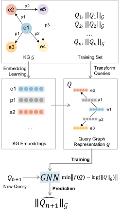
Figure 1: Overview of the GNCE framework. Given a Knowledge Graph, Embeddings are learned for all existing atoms. Next, a GNN is trained on a set of representative queries over this KG. The Queries are represented using the embeddings and the occurrence of each atom. Finally, the trained model is used to estimate the cardinality of new queries.

4.2 GNCE Architecture

Model Overview. In order to approximate the complex distribution in Eq. (7), we choose a neural network for representing it, due to its ability to learn complex functions (Maiorov and Pinkus, 1999). Since queries over KGs naturally represent graphs, an appropriate model choice is a graph neural network (GNN). Hence, the core of our approach is a GNN that, given the featurization $\mathcal{Q}$ of the query $Q$, directly predicts the cardinality of the related query. By that, we have a model that is invariant to a permutation of the nodes in the query graph and, in turn, parameter and data efficient.

An overview of our approach is shown in Figure 1. Given a KG $\mathcal{G}$ that we want to estimate query cardinalities over, we first calculate embeddings for all atoms in $\mathcal{G}$. Secondly, we create a query set consisting of queries and the corresponding cardinalities, for training our GNN to predict the cardinalities given the query, which we denote $\widehat{||Q||}_{\mathcal{G}}$. We represent the query as the corresponding query graph, where the atoms are represented by their corresponding embedding. Since, as explained in Section 2.2, RDF2Vec embeddings encode relatedness and joint probability, we choose it as our embedding method. Furthermore, since embeddings can be calculated incrementally for new atoms added to the KG, our resulting GNN will be inductive, i.e., it can make accurate cardinality estimates on unseen atoms (validated in Section 5.5). Next, we train the GNN on the query representations such that the difference between the predicted cardinality and the true cardinality gets minimized (cf. Model Training and Predictions). Finally, the trained GNN model can be used to predict the cardinality of new queries.

Model Definition.

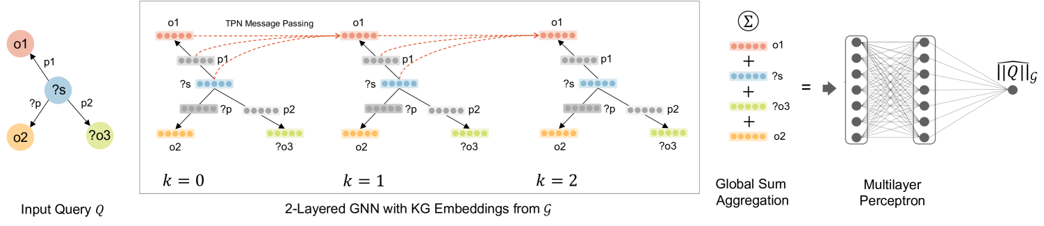
Figure 2: Architecture of the GNN for cardinality estimation. An initial query is represented by entity- and predicate embeddings and the connectivity between those atoms. For clarity, the TPN aggregation is only shown for one node. After node aggregation, the complete query graph is represented by summing all node embeddings. Finally, the query cardinality is estimated by mapping the query representation through a multilayer perception to a single dimension.

A detailed view of our GNN architecture is displayed in Figure 2. A given query $Q$ (with variables denoted by ’?’) is represented by the corresponding query graph and embeddings of the atoms. This representation is the input to our GNN ($k=0$). First, 2 Message Passing Layers ($k=1,k=2$) are applied to the input. In a preliminary experiment, we found that using more than 2 layers does not improve the performance of the model. Possible explanations for this are that 1.) the query graphs are rather small so 2 steps of message-passing are sufficient, and 2.) fewer layers avoid the oversmoothing problem (Chen et al., 2020), where node representations become increasingly similar, which deteriorates the model performance.

Our custom Message Passing function, which we term TPN Message Passing, is a modulation of the GINECONV (Hu et al., 2020) message passing function defined as

$$x_{i}^{(k)}=h_{\theta}^{(k)}\left((1+\epsilon)x_{i}^{(k-1)}+\sum_{j\in\mathcal{N}(i)}\mathrm{ReLU}(x_{j}^{(k-1)}+e_{j,i})\right)$$ (8)

We initially evaluated several different Message Passing Layers but found GINECONV to be superior to the others. This is in line with the theoretical findings from (Xu et al., 2019), which states that GINECONV is strictly more expressive than all other Message Passing Layers. It also aligns with results from LSS (Zhao et al., 2021), which also uses GINECONV as the Message Passing Function.

In Eq. (8), each $h_{\theta}^{(k)}$ is a multilayer perception with a ReLU Activation function. $\mathcal{N}(i)$ are all neighboring nodes of node $i$ with corresponding edges $e_{j,i}$. The parameter $\epsilon$ is an optionally learnable parameter that defaults to 0. Therefore, this function first sums up the neighboring nodes and edges individually, then aggregates those and the current representation of the node $x_{i}^{(k-1)}$ again through summation to finally transform them nonlinearly through $h_{\theta}$. Unfortunately, this Message Passing function treats the graph as undirected, as it aggregates the neighbors invariant under the direction of the edge. However, in cardinality estimation, the edge direction is of crucial information: The triples $(s\rightarrow p\rightarrow o)$ and $(o\rightarrow p\rightarrow s)$ can have vastly different cardinalities. One option to make the message passing directional is to only aggregate incoming edges at each node, i.e., instead of summing over $\mathcal{N}(i)$, summation happens over $\mathcal{N}^{+}(i)$. However, we found that this yields worse results than just summing over $\mathcal{N}(i)$, presumably because it restricts information flow. Hence, we use the following customized message passing function:

Definition 4.1 (TPN Message Passing).

The Triple Pattern Network (TPN) Message Passing transforms a node representation $x_{i}^{(k-1)}$ by separately transforming incoming messages (from $\mathcal{N}^{+}(i)$) and outgoing messages (from $\mathcal{N}^{-}(i)$) like

$$x_{i}^{(k)}=h_{\theta}^{(k)}\biggl{(}x_{i}^{(k-1)}\ +\sum_{j\in\mathcal{N}^{+}(i)}\mathrm{ReLU}(\mathbf{W}(x_{i}^{(k-1)}||e^{j,i}||x_{j}^{(k-1)}))\ +$$

$$\vspace{-3em}+\sum_{j\in\mathcal{N}^{-}(i)}\mathrm{ReLU}(\mathbf{W}(x_{j}^{(k-1)}||e^{i,j}||x_{i}^{(k-1)}))\biggr{)}$$

This function makes a case distinction between incoming and outgoing edges. Instead of aggregating the node and edge features through summation, we concatenate them ($||$) and linearly project them to the same dimensionality as $x_{i}$ using the matrix $\mathbf{W}$. The MLP $h_{\Theta}^{(k)}$ receives as input sums of the kind $\mathbf{O||P||S}$, where $\mathbf{O}$ is the feature of the node where the edge points to, $\mathbf{P}$ is the edge feature between the nodes, and $\mathbf{S}$ is the feature of the node where the edge originates.

After the graph nodes have been transformed by the two Message Passing layers, they need to be aggregated into a fixed-length vector. For that, we apply Global Sum Aggregation to them. That is, the representations of the nodes are summed up dimension-wise, resulting in a single vector $x$ with the same dimensionality as the node embeddings: $x=\sum_{l}x_{l}^{(k=2)}$.

Finally, this vector is transformed through a final 2-Layer MLP (with a ReLU activation in the hidden layer and linear activation in the final layer) into one single dimension. This dimension represents the predicted cardinality of the query.

Data and Featurization. In order to obtain a model that accurately predicts the cardinality of queries, it needs to be trained on a set of queries. For that, given a KG $\mathcal{G}$, we randomly sample queries according to some shape criterion (e.g. star/path with N triple patterns). It is important to sample uniformly across the KG in order to cover the distribution of data as best as possible and not only fit some regions of likely user queries.

For each query $Q$, we first calculate the individual occurrences $o(x)$ in $\mathcal{G}$ of each bound atom $x$ appearing in the queries. That is, the number of triples in $\mathcal{G}$ this atom occurs in any position, i.e., subject, predicate, or object. In Section 4.1, we saw that those quantities are part of the joint probability and, thus, will be informative to the approximation of the overall query cardinality. This is intuitively clear: the higher the number of atom occurrences, the higher the prior probability that a subgraph of $\mathcal{G}$ will match the query graph. As the $o(x)$ values are easy to obtain, it is much better to provide them to the model instead of the model having to learn them. Note also that removing them would make the model non-inductive, as the embeddings presumably do not encode that value.

Next, we calculate embeddings $e(x)$ for all occurring atoms in $Q$ using RDF2Vec. Note that we are only training on the entities occurring in our queries instead of the full KG, which greatly improves training speed for large graphs.

As the final input feature $i(x)$ for each atom, we use the concatenation of embedding and occurrence, i.e., $i(x)=e(x)||o(x)$. The featurization $\mathcal{Q}$ of the query is then given by the $i(x),\forall x$.

Variable atoms in the query graph require a special vector representation. First, we assign a numerical id to each variable. Then, we build the vectors as follows. The first dimension of the vector is set to the id. The rest of the dimensions are all set to $1$.

Model Training and Predictions. As mentioned above, our GNN is trained on the provided set of queries and true cardinalities. We aim to minimize the difference between the predicted cardinality and the true value. For that, as loss function, we employ the Mean Average Error (MAE) between our model output $f(\mathcal{Q})$ and the logarithm of the true cardinality $||Q||_{\mathcal{G}}$: $\mathcal{L}=||f(\mathcal{Q})-\log(||Q||_{\mathcal{G}})||$. Thus, the model learns to predict logarithms of cardinalities, which stabilizes the training due to the large range of possible cardinalities. Although the model is evaluated in terms of q-Error, we found that using MAE as a loss function yields better results than using q-Error directly. We train the model with a batch size of $32$ and for 100 epochs in all experiments. For optimization of the network, we use the Adam optimizer (Kingma and Ba, 2015) with a learning rate of $e^{-4}$. After training, given the featurization of a new query, the model can directly be used to predict the cardinality of that query.

Table 2: Dataset characteristics

KG	Triples	Entities	Predicates	Classes	Typed Entities
SWDF	242256	76711	170	118	28%
LUBM	2688849	664048	18	15	66%
YAGO	58M	13M	92	189K	98%

Table 3: Datasets and queries used for training and evaluating the approaches, grouped by the number of triples per query

KG	Star Queries				Path Queries
SWDF	Overall: 116645				Overall: 60739
	2tp	3tp	5tp	8tp	2tp	3tp	5tp	8tp
	27843	29461	29690	29651	538	19033	550	40618
LUBM	Overall: 113855				Overall: 55336
	2tp	3tp	5tp	8tp	2tp	3tp	4tp	8tp
	25356	29127	29727	29645	17784	33047	4505	0
YAGO	Overall: 91162				Overall: 87775
	2tp	3tp	5tp	8tp	2tp	3tp	5tp	8tp
	13968	24416	24509	28269	19378	33807	17990	16600

5 Experiments

We empirically assess the performance of GNCE for cardinality estimation. Concretely, we want to investigate the following questions: Q1 What is the effectiveness of GNCE compared to related methods? Q2 Does GNCE generalize to unseen entities? Q3 How does the prediction time of GNCE compare to the other methods?
The raw datasets, queries, results, and code to reproduce the plots are available on GitHub.

5.1 Experimental Setup

Datasets and Queries. We evaluate our approach on SWDF (Möller et al., 2007), LUBM (Guo et al., 2005), and YAGO (Suchanek et al., 2008). For LUBM and SWDF, we use the datasets provided in the supplementary material by Davitkova et al. (Davitkova et al., 2022). For YAGO, we use the dataset provided by the benchmark tool G-CARE (Park et al., 2020). LUBM is a synthetic benchmark modeling a university domain. SWDF is a small size but dense real-world dataset that models authors, papers, and conferences. Lastly, YAGO is a larger KG comprising common human knowledge. Table 2 summarizes the statistics about these datasets. We generate star and path queries with 2-8 triple patterns for each dataset, resulting in varying numbers of queries (see Table 3). The code for query generation can also be found on GitHub. The cardinality of the queries is in the range $[e^{0},e^{6}]$ for LUBM and SWDF, and $[e^{0},e^{8}]$ for YAGO. We randomly shuffle all queries and use 80% of them for training and evaluate all approaches on the remaining 20%.

Compared Methods. We compare GNCE to summary-based approaches (SUMRDF (Stefanoni et al., 2018) and Characteristic Sets (CSET) (Neumann and Moerkotte, 2011)), sampling-based approaches (impr (Chen and Lui, 2017), Wanderjoin (Li et al., 2016), and jsub (Zhao et al., 2018)), and learning-based approaches (LMKG (Davitkova et al., 2022) and LSS (Zhao et al., 2021)). For the sampling-based approaches, we report on their average performance of using 30 different samples (the default setting in G-CARE. For the learning-based approaches, we trained one model per dataset and query type and set up the number of parameters as recommended by the authors. The following table summarizes the number of parameters for the learning-based approaches per dataset. Note that GNCE has the lowest number of parameters, with 18x less compared to LSS. A smaller number of parameters typically means a smaller memory footprint of the approach as well as a faster execution time. It also indicates that the model’s inductive bias aligns better with the problem’s underlying nature and is less prone to overfitting.

Number of model parameters
KG GNCE (Ours) LMKG LSS SWDF $1.2\cdot e^{5}$ $4.5\cdot e^{5}$ $2.2\cdot e^{6}$ LUBM $1.2\cdot e^{5}$ $2.9\cdot e^{5}$ $2.2\cdot e^{6}$ YAGO $1.2\cdot e^{5}$ $3.8\cdot e^{5}$ $2.2\cdot e^{6}$

Implementation Details. GNCE is implemented using Python 3.8 and Pytorch Geometric (Fey and Lenssen, 2019) and the source code is available at GitHub. For computing the RDF2Vec embeddings, we use the implementation by Vandewiele et al. (Vandewiele et al., 2022). Here, we used an embedding dimension of 100 for GNCE. For the non-learning-based approaches, we use the implementation provided by G-CARE. All experiments, except for LSS on YAGO, have been conducted on a machine with 16 GB RAM, Intel Core i7-11800H @ 2.30GHz and an NVIDIA GeForce RTX 3050 GPU. Since LSS requires extensive amounts of RAM as it loads the whole KG into memory for training, it was trained on a machine with 512 GB of RAM,an Intel Xeon Silver 4314 CPU @ 2.40GHz as well as an Nvidia A100 GPU.

Evaluation Metrics. Similar to previous works (Zhao et al., 2021), we evaluate the effectiveness of the approaches in terms of the q-Error between the true cardinality and the predicted cardinality:

$$\text{q-Error}(Q)=\max\left(\frac{||Q||_{\mathcal{G}}}{\widehat{||Q||}_{\mathcal{G}}},\frac{\widehat{||Q||}_{\mathcal{G}}}{||Q||_{\mathcal{G}}}\right)$$ (9)

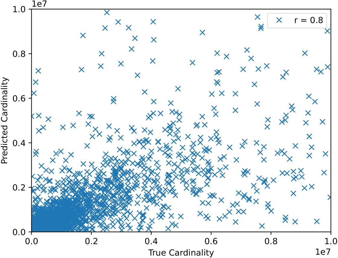
(a) GNCE

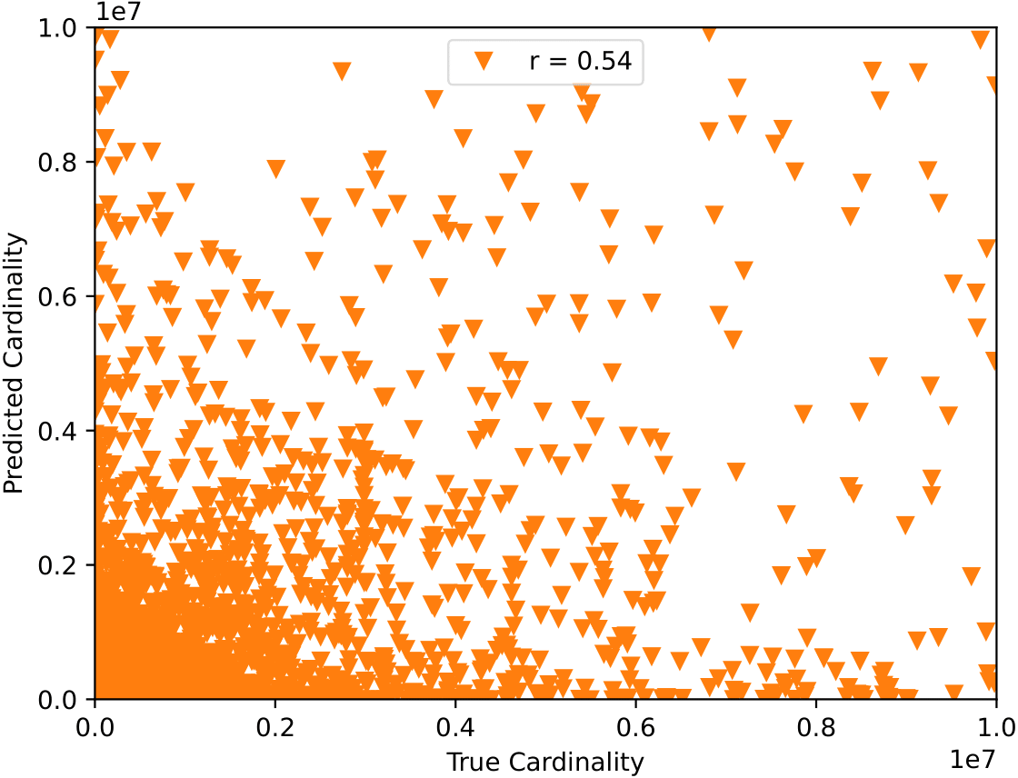
(b) LMKG

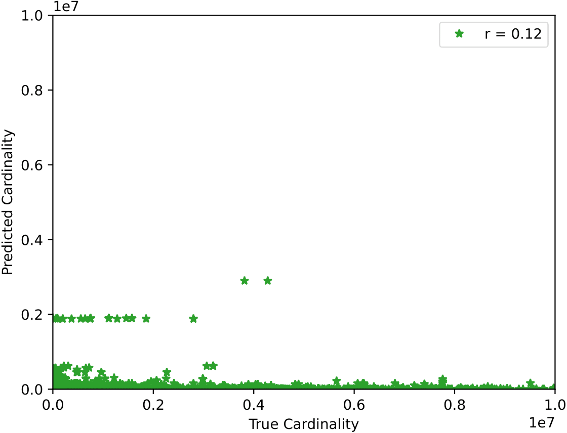
(c) LSS

Figure 3: Overall performance of learned approaches. The Plots show true and predicted cardinalities for learned approaches and correlation $r$. Queries across all datasets and query types are combined per approach.

5.2 Overview: Results of Learned Approaches

In this section, we look at the initial impressions on the effectiveness of the learned approaches (Q1), which are the closest to our work. Per approach, Figure 3 shows scatterplots of the true and predicted cardinalities for queries with a cardinality of up to $e^{6}$.

Overall, GNCE performs the best among the three methods as a clear correlation between prediction and true cardinality can be observed. The reported Pearson correlation coefficients also indicate that the correspondence between predicted and true cardinality is significantly higher for GNCE ($r=0.8$). LMKG also exhibits a moderate correlation ($r=0.54$), but also a significant amount of strong over-and underestimations. The situation is qualitatively different for LSS. Here, queries in the small cardinality range are overestimated, while queries in the moderate to higher cardinality range are severely underestimated. This behavior is also reflected in the low correlation coefficient of LSS ($r=0.12$).

To better understand how those initial impressions translate into q-Error, and how the methods perform within different ranges of the true cardinalities, we investigate the performance of all approaches for star queries (§ 5.3) and path queries (§ 5.4) separately.

5.3 Cardinality Estimation for Star Queries

In this section, we study the effectiveness of the approaches (Q1) for star queries, where the subject position is the join variable.
In Table 4, we report the mean q-Error of all approaches in each dataset. Overall, we observe that the q-Error increases along with the size of the KGs. This behavior is expected, as capturing correlations in larger datasets is more challenging, and queries with large cardinalities naturally occur more frequently in these datasets. These aspects negatively impact the estimations. The sampling and summary methods behave similarly to some extent, except for jsub which produces large errors in YAGO. CSET does not perform well in the tested star queries as these may have bound objects, which can create overestimations in CSET. Among the learned approaches, GNCE exhibits the best overall performance. Interestingly, LSS does not perform well in these KGs. We hypothesize that this is because the learned node representations based on classes of LSS cannot distinguish between queries with similar shapes but with different cardinalities. This behavior of LSS is clearly observed in the results for SWDF. While all the other approaches achieve their best performance in SWDF (smallest dataset), LSS produces large q-Errors because the number of typed entities is considerably small (only 22%, cf. Table 2). In the case of untyped entities, the LSS entity representation defaults to a generic vector of zeros, which does not contain any information. In contrast, GNCE does not make any assumption about the types of entities, and can still encode them through the embeddings if available.

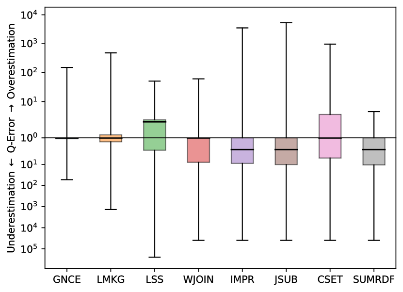
(a) SWDF

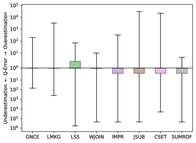
(b) LUBM

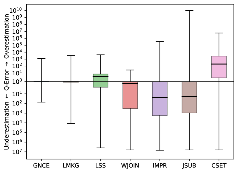
(c) YAGO

Figure 4: Boxplots of q-Errors of star queries

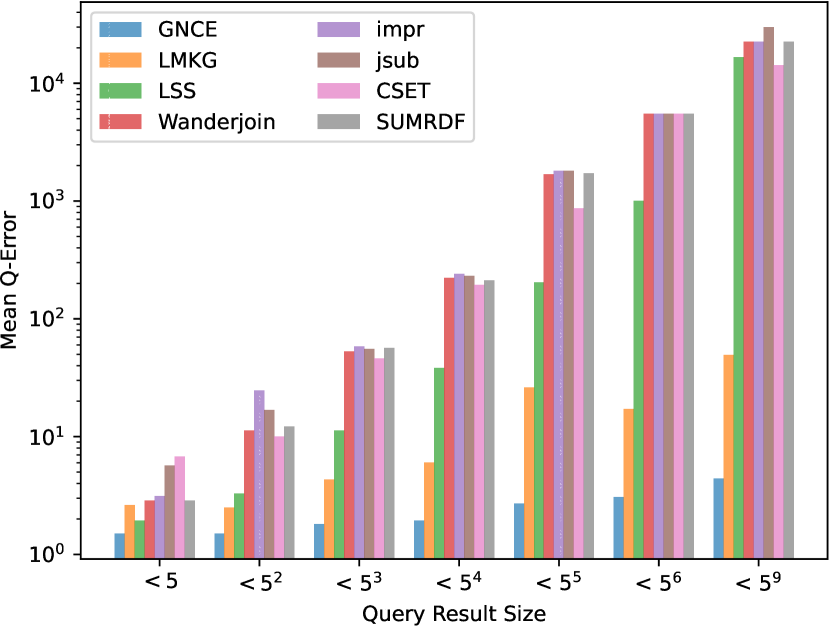
(a) SWDF

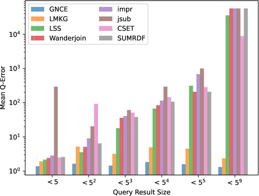
(b) LUBM

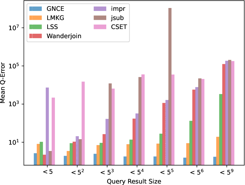
(c) YAGO

Figure 5: q-Errors for star-shaped queries, grouped by the true cardinalities of the queries

Table 4: Mean q-Errors for path queries

		Star Queries			Path Queries
	Approach	SWDF	LUBM	YAGO	SWDF	LUBM	YAGO
Sampling	WanderJoin	129	232	18713	21.7 $\cdot e^{4}$	388.9	9730
	impr	141	237	2605	$73.7\cdot e^{4}$	428.7	1722
	jsub	169	409	15 $\cdot e^{6}$	$37.4\cdot e^{4}$	414.36	10952
Summary	CSET	94	904	41586	$1.2\cdot e^{47}$	$63\cdot e^{10}$	$2.2\cdot e^{29}$
	SUMRDF	130	233	-	$2\cdot e^{5}$	$393\cdot e^{6}$	-
Learned	LMKG	2.7	1.85	8.78	1819.9	2.37	69
	LSS	1187	283	502.1	1187.1	179	1075
	GNCE	1.42	1.22	1.96	12.5	1.14	3.78

To further understand the performance of the approaches, we analyze the distributions of q-Errors. Figure 4 shows the distribution of q-Errors as boxplots; under- and overestimations are depicted by values below and above the horizontal line (perfect q-Error), respectively. We start by looking at the sampling methods (Wanderjoin, impr, and jsub), which tend to underestimate the cardinalities, in particular impr. This behavior was already observed by Park et al. (Park et al., 2020) for other datasets. The summary-based approaches also tend to produce underestimations, except for CSET in YAGO. A closer inspection of the results reveals that CSET largely overestimates the cardinalities for highly selective queries with bound objects. For the learned-based methods, the q-Errors are concentrated around the optimal value of 1 for GNCE and LMKG. LSS tends to overestimate slightly on large parts of the queries, but also shows severe underestimation (consistent with the results from Section 5.2). In comparison to LSS and LMKG, the maximum under-and overestimations of GNCE, as well as the quantiles, are more symmetric around the origin than for the other methods, indicating a more stable behavior across all datasets.

Next, we analyze the average q-Error of the approaches at different cardinality sizes (cf. Figure 5). The results show that the q-Error grows with increasing query cardinality, except for GNCE and LMKG. Non-learning-based approaches exhibit good performance in highly-selective queries with a result size range < 5. These queries typically have many bound atoms, for which sampling-based methods like impr and Wanderjoin might have collected (nearly) exact statistics. The only exception is CSET in YAGO, yet, these results are due to the large q-Errors produced by overestimations of CSET in highly-selective queries as previously explained. For learning-based approaches, the low number of training queries in the higher cardinality range can contribute to large errors. Still, GNCE, with its inductive bias tailored to the graph nature of queries and more informative feature representation due to embeddings, requires less training data to produce accurate predictions. For this reason, GNCE consistently has the lowest q-Error across all result sizes, with the only exception being the result size range < 5 in YAGO, where it is slightly outperformed by Wanderjoin.

5.4 Cardinality Estimation for Path Queries

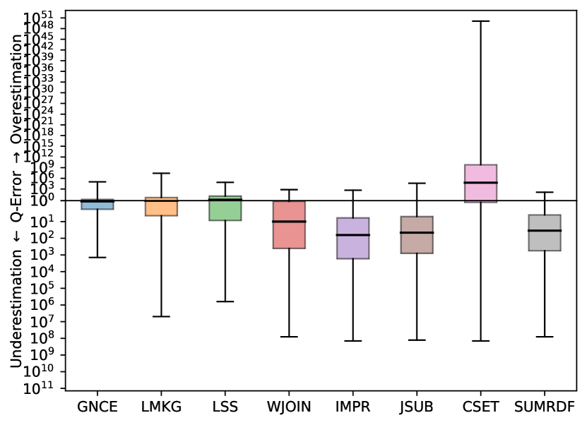
(a) SWDF

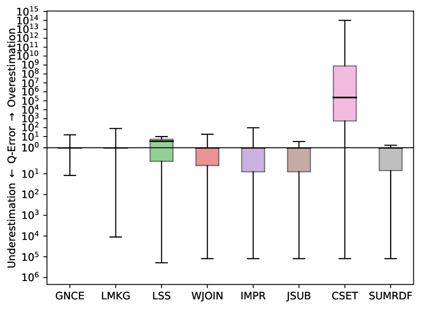
(b) LUBM

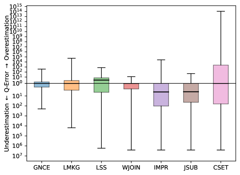
(c) YAGO

Figure 6: Boxplots of q-Errors for path queries

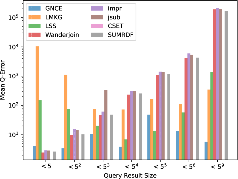
(a) SWDF

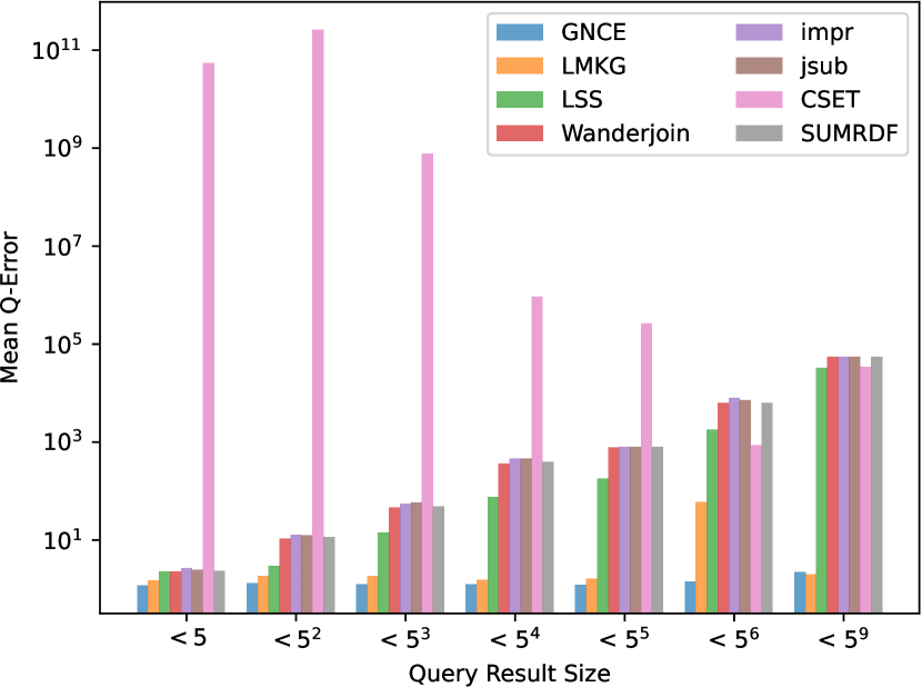
(b) LUBM

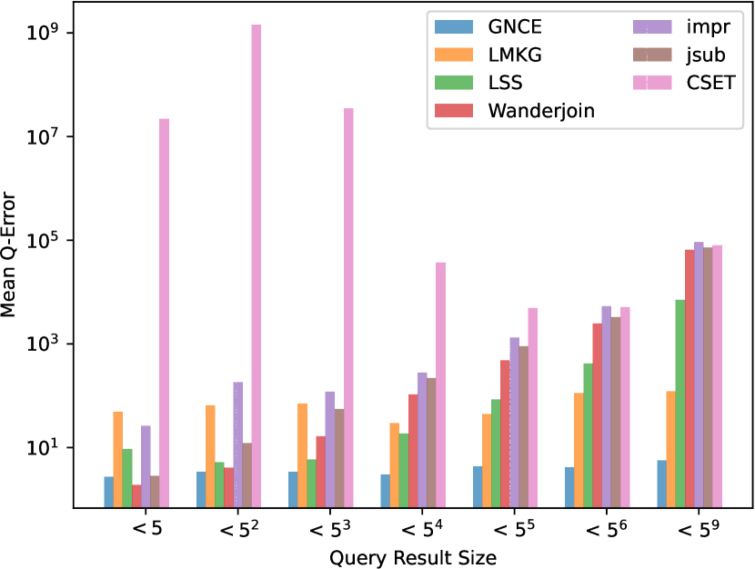
(c) YAGO

Figure 7: q-Errors for path queries, grouped by the true cardinalities of the queries

Next, we examine the effectiveness of the approaches (Q1) for path queries, with joins occurring between subjects and objects of triple patterns. We begin by analyzing the mean q-Error of the approaches, as presented in Table 4. The first observation is that all methods have higher q-Errors in comparison to the star-shaped queries (cf. Table 4). This is consistent with previous results reported by Park et al. (Park et al., 2020). Also interestingly, all methods are at least an order of magnitude worse on SWDF compared to the other datasets. This can be due to the high density of the SWDF graph, i.e., there are lots of possible paths from each start point which makes cardinality estimation significantly more error-prone. The effectiveness of the learning-based approaches is also affected by the fewer (training) queries in the dataset (cf. Table 3). Overall, the learned approaches exhibit the best performance, followed by sampling-based methods, and lastly summary-based methods. Still, GNCE outperforms the state of the art in path queries by several orders of magnitude.

Next, we analyze the distribution of q-Errors in Figure 6. All the sampling methods tend to underestimate the query cardinalities, especially in SWDF as previously explained due to the density of this dataset. Furthermore, their performance greatly deteriorates for YAGO (in comparison to LUBM) due to the size and the known semi-structuredness of this KG. In the summary-based approaches, the estimates computed by CSET are unrealistically high, a phenomenon that was already reported by Davitkova et al. (Davitkova et al., 2022). These results confirm that CSET summaries do not perform well at capturing join correlations between subjects and objects, as expected. In the learning-based approaches, LSS tends to produce overestimations. This was already observed in the star queries (cf. Section 5.3), indicating that this is a recurrent behavior of LSS. In contrast, both GNCE and LSS tend to underestimate. Still, the spread of the errors shown by the whiskers is smaller for GNCE than LMKG.

In Figure 7, we examine the q-Errors categorized by query cardinality. Please note that in Figure 7(a), the bars for CSET are omitted due to the extremely high values. Similar to the trend observed for star-shaped queries, we found that the q-Error increases with the cardinality of queries for all approaches except for GNCE, which exhibited a mostly consistent mean q-Error. Second, in SWDF and YAGO, the sampling-based methods marginally outperform GNCE in the small cardinality range <5. Interestingly, on SWDF, for queries with cardinalities between $5^{4}$ and $5^{5}$, LSS performs best out of all approaches in this particular case.

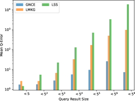
Figure 8: Mean q-Errors on queries consisting of unseen entities for star-shaped queries on the SWDF dataset.

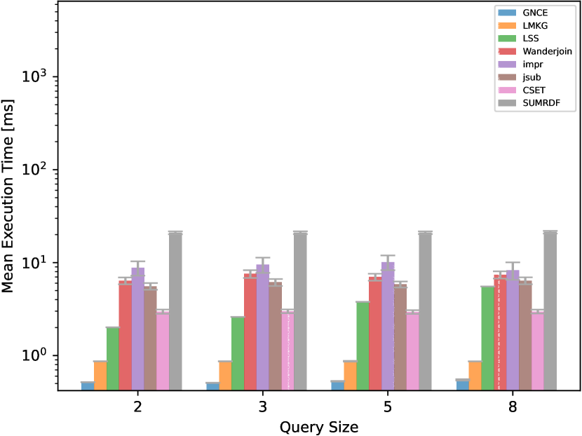
(a) SWDF - Star

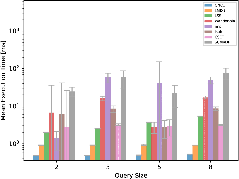
(b) SWDF - Path

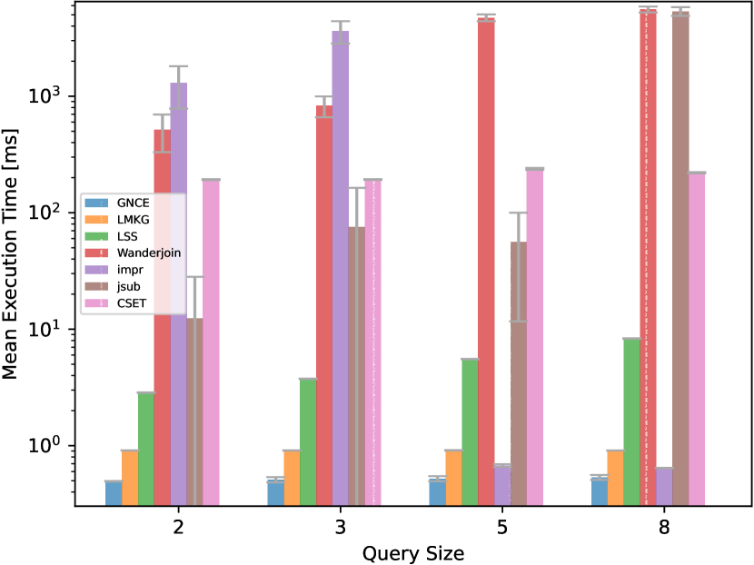
(c) YAGO - Star

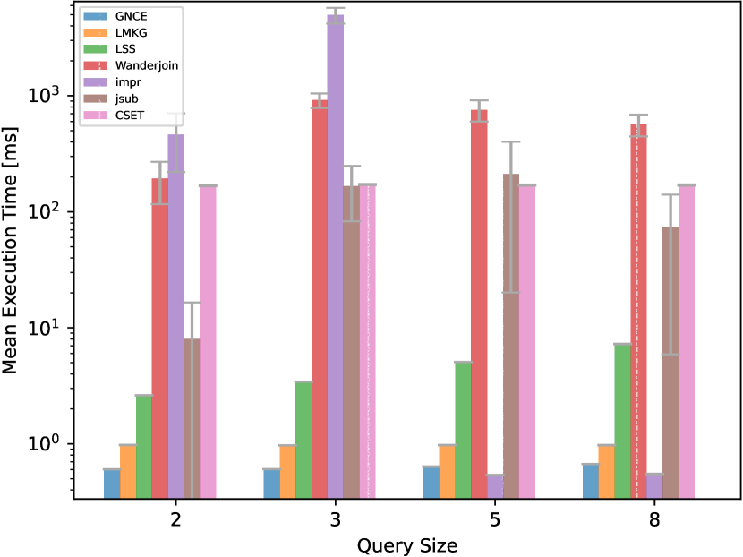
(d) YAGO - Path

Figure 9: Mean execution time [ms] of the different approaches, grouped by the number of triple patterns in the query. Confidence intervals (95%) are shown in grey bars

5.5 Inductive Case: Results of Learned Approaches

In this section, we assess the effectiveness of learned approaches in the inductive case (Q2), i.e., when test queries involve atoms that were not seen during training. For the sake of space, we conduct this experiment only on star queries for SWDF and proceeded as follows. The query set was partitioned into two disjoint sets, such that the entities in both sets were mutually exclusive, i.e., each query in one set did not involve any entity present in the other set. This resulted in two sets with 111K and 2.1K queries each. Then, we trained the three learned approaches, GNCE, LMKG, LSS, on the larger of the two sets and evaluate on the other. The average of q-Errors of the approaches is presented in Figure 8.

Compared to the non-inductive case in Figure 5(a), all methods experience a performance deterioration. However, the increase of the q-Error is significantly smaller for GNCE compared to the other two methods. One notable observation in Figure 8 is that for queries with a cardinality smaller than $5^{2}$, the performance of LSS is improved in comparison to its performance in the non-inductive case. This is because the test set primarily consists of queries with two triple patterns – as it is hard to find larger queries that do not contain entities from the other set – which are easier to evaluate for LSS. For LMKG, the inductive case is challenging as its architecture completely relies on node representations computed from the queries seen during training, while GNCE and LSS use (knowledge) graph embeddings. Because of this, LMKG is the method affected the most in the inductive case. In summary, the results of this experiment show that GNCE can be used in the inductive setting, when new queries are constantly processed, without frequently retraining the model.

5.6 Prediction Efficiency

To be of practical use during query optimization, a cardinality estimator needs to produce results with minimal runtime (Q3). Therefore, in this experiment, we measure the runtime of prediction for the different queries from the smallest and largest datasets, i.e., SWDF and YAGO. To measure the runtime we use the time library (Foundation, 2021) in python. For the learned techniques, we evaluate the propagation of the query representation through the network’s forward pass. For the methods provided by G-CARE (Park et al., 2020), we use the implemented evaluate function of the different methods. All measurements were performed on the same machine, except for LSS on YAGO, which had to be executed on the larger cluster (described in Section 5.1).

We present the results in Figure 9, grouped by the number of triple patterns in the query (query size). The grey bars indicate the 95% confidence interval of the data.

Comparing the results between SWDF and YAGO, we observe that the runtime of the non-learning-based approaches is impacted by the size of the dataset as well as the type of query. The sample-based methods, i.e. impr, jsub, and WanderJoin, show higher efficiency mainly on the smaller SWDF dataset. The performance of CSET and RDFSUM is similar to the sample-based approaches, as they require several accesses to (large) summaries to perform the predictions. Among the learned methods, GNCE consistently has the lowest runtime. From the learned approaches, we report stable behavior across the datasets, query sizes, and types. This is observed in both the mean values as well as the narrow confidence interval indicating almost no variations in prediction time. In particular, GNCE exhibits the best performance from the learned approaches and even outperforms the majority of the non-learning ones except for impr on YAGO. Overall, the runtime of GNCE is competitive with other established methods and is small enough to be employed in a real-time query optimization setting. It is noteworthy that these measurements were obtained using unoptimized prototypical code. In a production environment, neural networks are typically compiled, which results in a further reduction of execution time.

6 Conclusion and Outlook

In this work, we presented GNCE, a novel method for accurate cardinality estimation over Knowledge Graphs (KG) based on KG Embeddings and Graph Neural Networks (GNN). The Embeddings are used to provide semantically meaningful features to the GNN, which directly predicts the cardinality of the embedding-enhanced query graph. By design, our method is lightweight, tailored to the graph structure of queries, requires few training data, and allows for inductive generalization to unseen entities.

On differently sized real-world datasets and a synthetic benchmark, our approach consistently outperforms the state-of-the-art LSS and LMKG in terms of q-Error over different query shapes and sizes. GNCE is also robust in the sense that it does not produce severe prediction errors. An experiment on inductive cases shows that GNCE generalizes to unseen entities, making it a suitable solution for actual deployment in a quickly changing query processing setting. In that context, we also showed that our model is lightweight with fewer parameters than all other learned approaches, leading also to smaller and almost constant runtime for predictions below 1 ms.

Further research directions include the transferability of one model to other datasets, to minimize the training efforts. We also plan to deploy GNCE in a query optimizer to test its effect on actual query execution time as well as ease of integration and operationality in a real-world setting.

References

- Noy et al. [2019] Natasha Noy, Yuqing Gao, Anshu Jain, Anant Narayanan, Alan Patterson, and Jamie Taylor. Industry-scale knowledge graphs: Lessons and challenges. Commun. ACM, 62(8):36–43, jul 2019. ISSN 0001-0782. doi:10.1145/3331166. URL https://doi.org/10.1145/3331166.
- Prud’hommeaux and Seaborne [2008] Eric Prud’hommeaux and Andy Seaborne. SPARQL query language for RDF. W3C recommendation, W3C, January 2008. https://www.w3.org/TR/2008/REC-rdf-sparql-query-20080115/.
- Francis et al. [2018] Nadime Francis, Alastair Green, Paolo Guagliardo, Leonid Libkin, Tobias Lindaaker, Victor Marsault, Stefan Plantikow, Mats Rydberg, Petra Selmer, and Andrés Taylor. Cypher: An evolving query language for property graphs. In Proceedings of the 2018 International Conference on Management of Data, pages 1433–1445, 2018.
- Neumann and Moerkotte [2011] Thomas Neumann and Guido Moerkotte. Characteristic sets: Accurate cardinality estimation for RDF queries with multiple joins. In Serge Abiteboul, Klemens Böhm, Christoph Koch, and Kian-Lee Tan, editors, Proceedings of the 27th International Conference on Data Engineering, ICDE 2011, April 11-16, 2011, Hannover, Germany, pages 984–994. IEEE Computer Society, 2011. doi:10.1109/ICDE.2011.5767868. URL https://doi.org/10.1109/ICDE.2011.5767868.
- Stefanoni et al. [2018] Giorgio Stefanoni, Boris Motik, and Egor V. Kostylev. Estimating the cardinality of conjunctive queries over rdf data using graph summarisation. pages 1043–1052. Association for Computing Machinery, Inc, 4 2018. ISBN 9781450356398. doi:10.1145/3178876.3186003.
- Davitkova et al. [2022] Angjela Davitkova, Damjan Gjurovski, and Sebastian Michel. Lmkg: Learned models for cardinality estimation in knowledge graphs. 2022. doi:10.48786/edbt.2022.07. URL https://www.w3.org/TR/sparql11-overview/.
- Zhao et al. [2021] Kangfei Zhao, Jeffrey Xu Yu, Hao Zhang, Qiyan Li, and Yu Rong. A learned sketch for subgraph counting. pages 2142–2155. Association for Computing Machinery, 2021. doi:10.1145/3448016.3457289.
- Xu et al. [2019] Keyulu Xu, Weihua Hu, Jure Leskovec, and Stefanie Jegelka. How powerful are graph neural networks? In 7th International Conference on Learning Representations, ICLR 2019, New Orleans, LA, USA, May 6-9, 2019. OpenReview.net, 2019. URL https://openreview.net/forum?id=ryGs6iA5Km.
- Rossi et al. [2021] Andrea Rossi, Denilson Barbosa, Donatella Firmani, Antonio Matinata, and Paolo Merialdo. Knowledge graph embedding for link prediction: A comparative analysis. ACM Transactions on Knowledge Discovery from Data, 15, 1 2021. ISSN 1556472X. doi:10.1145/3424672.
- Hogan et al. [2022] Aidan Hogan, Eva Blomqvist, Michael Cochez, Claudia d’Amato, Gerard de Melo, Claudio Gutierrez, Sabrina Kirrane, José Emilio Labra Gayo, Roberto Navigli, Sebastian Neumaier, Axel-Cyrille Ngonga Ngomo, Axel Polleres, Sabbir M. Rashid, Anisa Rula, Lukas Schmelzeisen, Juan F. Sequeda, Steffen Staab, and Antoine Zimmermann. Knowledge graphs. ACM Comput. Surv., 54(4):71:1–71:37, 2022. doi:10.1145/3447772. URL https://doi.org/10.1145/3447772.
- Cyganiak et al. [2014] Richard Cyganiak, David Wood, and Markus Lanthaler. RDF 1.1 concepts and abstract syntax. W3C recommendation, W3C, February 2014. https://www.w3.org/TR/2014/REC-rdf11-concepts-20140225/.
- Angles [2018] Renzo Angles. The property graph database model. In AMW, 2018.
- Ristoski and Paulheim [2016] Petar Ristoski and Heiko Paulheim. RDF2Vec: RDF graph embeddings for data mining. In International Semantic Web Conference, pages 498–514. Springer, 2016.
- Weller and Acosta [2021] Tobias Weller and Maribel Acosta. Predicting instance type assertions in knowledge graphs using stochastic neural networks. In Gianluca Demartini, Guido Zuccon, J. Shane Culpepper, Zi Huang, and Hanghang Tong, editors, CIKM ’21: The 30th ACM International Conference on Information and Knowledge Management, Virtual Event, Queensland, Australia, November 1 - 5, 2021, pages 2111–2118. ACM, 2021. doi:10.1145/3459637.3482377. URL https://doi.org/10.1145/3459637.3482377.
- Mikolov et al. [2013] Tomás Mikolov, Kai Chen, Greg Corrado, and Jeffrey Dean. Efficient estimation of word representations in vector space. In Yoshua Bengio and Yann LeCun, editors, 1st International Conference on Learning Representations, ICLR 2013, Scottsdale, Arizona, USA, May 2-4, 2013, Workshop Track Proceedings, 2013. URL http://arxiv.org/abs/1301.3781.
- Bronstein et al. [2021] Michael M. Bronstein, Joan Bruna, Taco Cohen, and Petar Veličković. Geometric deep learning: Grids, groups, graphs, geodesics, and gauges. 4 2021. URL http://arxiv.org/abs/2104.13478.
- Team [2022] PyG Team. Creating message passing networks. https://pytorch-geometric.readthedocs.io/en/latest/notes/create_gnn.html, 2022. Accessed: 2022-11-29.
- Wu et al. [2019] Zonghan Wu, Shirui Pan, Fengwen Chen, Guodong Long, Chengqi Zhang, and Philip S. Yu. A comprehensive survey on graph neural networks. 1 2019. doi:10.1109/TNNLS.2020.2978386. URL http://arxiv.org/abs/1901.00596http://dx.doi.org/10.1109/TNNLS.2020.2978386.
- Cormode et al. [2011] Graham Cormode, Minos Garofalakis, Peter J. Haas, and Chris Jermaine. Synopses for massive data: Samples, histograms, wavelets, sketches. Foundations and Trends in Databases, 4:1–294, 2011. ISSN 19317883. doi:10.1561/1900000004.
- Vengerov et al. [2150] David Vengerov, Andre Cavalheiro Menck, Mohamed Zait, and Sunil P Chakkappen. Join size estimation subject to filter conditions, 2150.
- Li et al. [2016] Feifei Li, Bin Wu, Ke Yi, and Zhuoyue Zhao. Wander join: Online aggregation via random walks. volume 26-June-2016, pages 615–629. Association for Computing Machinery, 6 2016. ISBN 9781450335317. doi:10.1145/2882903.2915235.
- Zhao et al. [2018] Zhuoyue Zhao, Robert Christensen, Feifei Li, Xiao Hu, and Ke Yi. Random sampling over joins revisited. In Proceedings of the 2018 International Conference on Management of Data, pages 1525–1539, 2018.
- Park et al. [2020] Yeonsu Park, Seongyun Ko, Sourav S. Bhowmick, Kyoungmin Kim, Kijae Hong, and Wook Shin Han. G-care: A framework for performance benchmarking of cardinality estimation techniques for subgraph matching. pages 1099–1114. Association for Computing Machinery, 6 2020. ISBN 9781450367356. doi:10.1145/3318464.3389702.
- Sun et al. [2021] Ji Sun, Jintao Zhang, Zhaoyan Sun, Guoliang Li, and Nan Tang. Learned cardinality estimation: A design space exploration and a comparative evaluation. volume 15, pages 85–97. VLDB Endowment, 2021. doi:10.14778/3485450.3485459.
- Getoor et al. [2001] Lise Getoor, Ben Taskar, and Daphne Koller. Selectivity estimation using probabilistic models, 2001.
- Tzoumas et al. [2011] Kostas Tzoumas, Amol Deshpande, and Christian S. Jensen. Lightweight graphical models for selectivity estimation without independence assumptions. Proceedings of the VLDB Endowment, 4:852–863, 8 2011. ISSN 21508097. doi:10.14778/3402707.3402724.
- Halford et al. [2019] Max Halford, Philippe Saint-Pierre, and Frank Morvan. An approach based on bayesian networks for query selectivity estimation. 7 2019. doi:10.1007/978-3-030-18579-4_1. URL http://arxiv.org/abs/1907.06295http://dx.doi.org/10.1007/978-3-030-18579-4_1.
- Hilprecht et al. [2020] Benjamin Hilprecht, Andreas Schmidt, Moritz Kulessa, Alejandro Molina, Kristian Kersting, and Carsten Binnig. Deepdb: Learn from data, not from queries! volume 13, pages 992–1005. VLDB Endowment, 2020. doi:10.14778/3384345.3384349.
- Kipf et al. [2019] Andreas Kipf, Thomas Kipf, Bernhard Radke, Viktor Leis, Peter A. Boncz, and Alfons Kemper. Learned cardinalities: Estimating correlated joins with deep learning. In 9th Biennial Conference on Innovative Data Systems Research, CIDR 2019, Asilomar, CA, USA, January 13-16, 2019, Online Proceedings. www.cidrdb.org, 2019. URL http://cidrdb.org/cidr2019/papers/p101-kipf-cidr19.pdf.
- Woltmann et al. [2019] Lucas Woltmann, Claudio Hartmann, Maik Thiele, Dirk Habich, and Wolfgang Lehner. Cardinality estimation with local deep learning models. Association for Computing Machinery, 7 2019. ISBN 9781450368025. doi:10.1145/3329859.3329875.
- Zhao et al. [2022] Kangfei Zhao, Jeffrey Xu Yu, Zongyan He, Rui Li, and Hao Zhang. Lightweight and accurate cardinality estimation by neural network gaussian process. In Proceedings of the 2022 International Conference on Management of Data, pages 973–987, 2022.
- Stocker et al. [2008] Markus Stocker, Andy Seaborne, Abraham Bernstein, Christoph Kiefer, and Dave Reynolds. Sparql basic graph pattern optimization using selectivity estimation. pages 595–604, 2008. ISBN 9781605580852. doi:10.1145/1367497.1367578.
- Shironoshita et al. [2007] E Patrick Shironoshita, Michael T Ryan, and Mansur R Kabuka. Cardinality estimation for the optimization of queries on ontologies. ACM SIGMOD Record, 36(2):13–18, 2007.
- Neumann and Weikum [2009] Thomas Neumann and Gerhard Weikum. The rdf-3x engine for scalable management of rdf data, 2009.
- Chen and Lui [2017] Xiaowei Chen and John C.S. Lui. Mining graphlet counts in online social networks. pages 71–80. Institute of Electrical and Electronics Engineers Inc., 1 2017. ISBN 9781509054725. doi:10.1109/ICDM.2016.99.
- Huang and Liu [2011] Hai Huang and Chengfei Liu. Estimating selectivity for joined rdf triple patterns. pages 1435–1444, 2011. ISBN 9781450307178. doi:10.1145/2063576.2063784.
- Zhang et al. [2019] Jie Zhang, Yuxiao Dong, Yan Wang, Jie Tang, and Ming Ding. Prone: Fast and scalable network representation learning. In Proceedings of the Twenty-Eighth International Joint Conference on Artificial Intelligence, IJCAI-19, pages 4278–4284. International Joint Conferences on Artificial Intelligence Organization, 7 2019. doi:10.24963/ijcai.2019/594. URL https://doi.org/10.24963/ijcai.2019/594.
- Wang et al. [2022] Hanchen Wang, Rong Hu, Ying Zhang, Lu Qin, Wei Wang, and Wenjie Zhang. Neural subgraph counting with wasserstein estimator. pages 160–175. Association for Computing Machinery, 6 2022. ISBN 9781450392495. doi:10.1145/3514221.3526163.
- Bengio et al. [2021] Emmanuel Bengio, Moksh Jain, Maksym Korablyov, Doina Precup, and Yoshua Bengio. Flow network based generative models for non-iterative diverse candidate generation. Advances in Neural Information Processing Systems, 34:27381–27394, 2021.
- Maiorov and Pinkus [1999] Vitaly Maiorov and Allan Pinkus. Lower bounds for approximation by mlp neural networks. Neurocomputing, 25(1-3):81–91, 1999.
- Chen et al. [2020] Deli Chen, Yankai Lin, Wei Li, Peng Li, Jie Zhou, and Xu Sun. Measuring and relieving the over-smoothing problem for graph neural networks from the topological view. In Proceedings of the AAAI conference on artificial intelligence, volume 34, pages 3438–3445, 2020.
- Hu et al. [2020] Weihua Hu, Bowen Liu, Joseph Gomes, Marinka Zitnik, Percy Liang, Vijay S. Pande, and Jure Leskovec. Strategies for pre-training graph neural networks. In 8th International Conference on Learning Representations, ICLR 2020, Addis Ababa, Ethiopia, April 26-30, 2020. OpenReview.net, 2020. URL https://openreview.net/forum?id=HJlWWJSFDH.
- Kingma and Ba [2015] Diederik P. Kingma and Jimmy Ba. Adam: A method for stochastic optimization. In Yoshua Bengio and Yann LeCun, editors, 3rd International Conference on Learning Representations, ICLR 2015, San Diego, CA, USA, May 7-9, 2015, Conference Track Proceedings, 2015. URL http://arxiv.org/abs/1412.6980.
- Möller et al. [2007] Knud Möller, Tom Heath, Siegfried Handschuh, and John Domingue. Recipes for semantic web dog food - the ESWC and ISWC metadata projects. In Karl Aberer, Key-Sun Choi, Natasha Fridman Noy, Dean Allemang, Kyung-Il Lee, Lyndon J. B. Nixon, Jennifer Golbeck, Peter Mika, Diana Maynard, Riichiro Mizoguchi, Guus Schreiber, and Philippe Cudré-Mauroux, editors, The Semantic Web, 6th International Semantic Web Conference, 2nd Asian Semantic Web Conference, ISWC 2007 + ASWC 2007, Busan, Korea, November 11-15, 2007, volume 4825 of Lecture Notes in Computer Science, pages 802–815. Springer, 2007. doi:10.1007/978-3-540-76298-0_58. URL https://doi.org/10.1007/978-3-540-76298-0_58.
- Guo et al. [2005] Yuanbo Guo, Zhengxiang Pan, and Jeff Heflin. LUBM: A benchmark for OWL knowledge base systems. J. Web Semant., 3(2-3):158–182, 2005. doi:10.1016/j.websem.2005.06.005. URL https://doi.org/10.1016/j.websem.2005.06.005.
- Suchanek et al. [2008] Fabian M. Suchanek, Gjergji Kasneci, and Gerhard Weikum. Yago: A large ontology from wikipedia and wordnet. Web Semantics, 6:203–217, 9 2008. ISSN 15708268. doi:10.1016/j.websem.2008.06.001.
- Fey and Lenssen [2019] Matthias Fey and Jan E. Lenssen. Fast graph representation learning with PyTorch Geometric. In ICLR Workshop on Representation Learning on Graphs and Manifolds, 2019.
- Vandewiele et al. [2022] Gilles Vandewiele, Bram Steenwinckel, Terencio Agozzino, and Femke Ongenae. pyrdf2vec: A python implementation and extension of rdf2vec. 2022. doi:10.48550/ARXIV.2205.02283. URL https://arxiv.org/abs/2205.02283.
- Zloch et al. [2019] Matthäus Zloch, Maribel Acosta, Daniel Hienert, Stefan Dietze, and Stefan Conrad. A software framework and datasets for the analysis of graph measures on rdf graphs. In The Semantic Web: 16th International Conference, ESWC 2019, Portorož, Slovenia, June 2–6, 2019, Proceedings 16, pages 523–539. Springer, 2019.
- Foundation [2021] Python Software Foundation. The Python Standard Library - time. https://docs.python.org/3/library/time.html, 2021. [Online; accessed 27-February-2023].