Auroral, Ionospheric and Ground Magnetic Signatures of Magnetopause Surface Modes
Abstract
Surface waves on Earth’s magnetopause have a controlling effect upon global magnetospheric dynamics. Since spacecraft provide sparse in situ observation points, remote sensing these modes using ground-based instruments in the polar regions is desirable. However, many open conceptual questions on the expected signatures remain. Therefore, we provide predictions of key qualitative features expected in auroral, ionospheric, and ground magnetic observations through both magnetohydrodynamic theory and a global coupled magnetosphere-ionosphere simulation of a magnetopause surface eigenmode. These show monochromatic oscillatory field-aligned currents, due to both the surface mode and its non-resonant Alfvén coupling, are present throughout the magnetosphere. The currents peak in amplitude at the equatorward edge of the magnetopause boundary layer, not the open-closed boundary as previously thought. They also exhibit slow poleward phase motion rather than being purely evanescent. We suggest the upward field-aligned current perturbations may result in periodic auroral brightenings. In the ionosphere, convection vortices circulate the poleward moving field-aligned current structures. Finally, surface mode signals are predicted in the ground magnetic field, with ionospheric Hall currents rotating perturbations by approximately (but not exactly) compared to the magnetosphere. Thus typical dayside magnetopause surface modes should be strongest in the East-West ground magnetic field component. Overall, all ground-based signatures of the magnetopause surface mode are predicted to have the same frequency across -shells, amplitudes that maximise near the magnetopause’s equatorward edge, and larger latitudinal scales than for field line resonance. Implications in terms of ionospheric Joule heating and geomagnetically induced currents are discussed.
Journal of Geophysical Research: Space Physics
Space and Atmospheric Physics Group, Department of Physics, Imperial College London, London, UK.
Space Science Institute, Boulder, Colorado, USA.
NASA Goddard Space Flight Center, Greenbelt, Maryland, USA.
Department of Mathematics and Statistics, University of St Andrews, St Andrews, UK.
Institut für Geophysik und extraterrestrische Physik, TU Braunschweig, Braunschweig, Germany.
Department of Electrical and Computer Engineering, Virginia Polytechnic Institute and State University, Blacksburg, Virginia, USA.
High Altitude Observatory, National Center for Atmospheric Research, Boulder, Colorado, USA.
Martin Archerm.archer10@imperial.ac.uk
Theory and global simulations of magnetopause surface waves’ effects on the aurorae, ionosphere, and ground magnetic field are investigated
We predict poleward-moving periodic aurora, convection vortices, and ground pulsations, with larger latitudinal scales than Alfvén modes
Amplitudes of all signals peak near the projection of the inner/equatorward edge of the magnetopause rather than the open–closed boundary
Plain Language Summary
Waves on the boundary of the magnetosphere, the magnetic shield established by the interplay of the solar wind with Earth’s magnetic field, play a controlling role on energy flow into our space environment. While these waves can be observed as they pass over satellites in orbit, due to the small number of suitable satellites available it would be helpful to be able to detect these waves from the surface of the Earth with instruments that measure the northern/southern lights, motion of the top of our atmosphere, or magnetic field on the ground. However, we do not currently understand what the signs of these waves should look like in such instruments. In this paper we develop theory and use computer simulations of these boundary waves to predict key features one might expect to measure from the ground. Based on these predictions, we also discuss how the waves might contribute to the hazards of space weather.
1 Introduction
The interaction between the solar wind and Earth’s magnetosphere results in a zoo of dynamical plasma waves. Those with wavelengths comparable to the size of the magnetosphere are well described by magnetohydrodynamics (MHD) and due to their corresponding frequencies, (Jacobs \BOthers., \APACyear1964), are known as ultra-low frequency (ULF) waves. ULF waves play important roles in space weather processes such as substorms (e.g. Kepko \BBA Kivelson, \APACyear1999), wave-wave (e.g. Li \BOthers., \APACyear2011) and wave-particle (e.g. Turner \BOthers., \APACyear2012) interactions, magnetosphere-ionosphere (MI) coupling (e.g. Keiling, \APACyear2009), and geomagnetically induced currents (e.g. Heyns \BOthers., \APACyear2021). In addition to familiar Alfvén and fast/slow magnetosonic body MHD waves (those which may freely propagate through plasma volumes), sharp discontinuities separating regions with different physical parameters, such as the magnetopause and plasmapause, allow for collective modes – surface waves (Kruskal \BBA Schwartzschild, \APACyear1954; Goedbloed, \APACyear1971; Chen \BBA Hasegawa, \APACyear1974). Surface modes lead to mass, momentum, and energy transport across the boundary, consequently manifesting a controlling effect on global magnetospheric wave dynamics (e.g. Kivelson \BBA Chen, \APACyear1995). As with the body waves, theory behind surface waves has largely been developed in simplified box model magnetospheres, typically with homogeneous half-spaces. Within these the surface mode is inherently compressional, being described by two evanescent fast magnetosonic waves (one in each half-space such that perturbations decay with distance from the boundary) that are joined by boundary conditions which ensure pressure balance and continuity of normal displacement across the interface (Pu \BBA Kivelson, \APACyear1983; Plaschke \BBA Glassmeier, \APACyear2011). On each side the magnetosonic relation
| (1) |
holds, where represents the direction normal to the discontinuity, and and are the Alfvén and sound speeds respectively (see Notation). Under incompressibility, the last term of equation 1 may be neglected and the normal wavenumber is imaginary. In contrast, if this assumption is not valid or if waves are damped/unstable then may be complex, exhibiting both evanescence and normal phase motion (Pu \BBA Kivelson, \APACyear1983; M\BPBIO. Archer \BOthers., \APACyear2021, hereafter A21). The dispersion relation for incompressible surface waves in a box model can be analytically solved. Applied to the magnetopause, for zero magnetic shear across boundary (equivalent to northward interplanetary magnetic field; IMF) and no background flows, it is (Plaschke \BBA Glassmeier, \APACyear2011)
| (2) |
where refers to the magnetosphere and the magnetosheath. The boundary conditions of closed magnetic field lines at the northern and southern ionospheres impose quantised wavelengths along the field (Chen \BBA Hasegawa, \APACyear1974), forming an eigenmode of the system. On the dayside, where magnetosheath flows are smaller, this magnetopause surface eigenmode (MSE) is expected to occupy frequencies below (Plaschke \BOthers., \APACyear2009; M\BPBIO. Archer \BBA Plaschke, \APACyear2015). Such low eigenfrequencies are a result of the combination of magnetic fields and densities from both sides of the magnetopause, making it the lowest frequency magnetospheric normal mode and highly penetrating. However, in the flanks the faster magnetosheath velocities are expected to dictate the wave frequency (Plaschke \BBA Glassmeier, \APACyear2011; O. Kozyreva \BOthers., \APACyear2019), rather than the extent of the field lines, yielding shorter wavelengths and periods. In the absence of continuous driving or instabilities, surface modes on a boundary of finite thickness are strongly damped, with this thought to be primarily due to mode conversion to Alfvén waves and spatial phase mixing within the boundary layer rather than dissipation in the ionosphere or due to the presence of the ionosphere-Earth boundary (Chen \BBA Hasegawa, \APACyear1974).
Magnetopause surface modes may be excited by several driving processes, either external or internal to the magnetosphere. External mechanisms include upstream (solar wind, foreshock, or magnetosheath) pressure variations, which may be either quasi-periodic (e.g. Sibeck \BOthers., \APACyear1989) or impulsive (e.g. Shue \BOthers., \APACyear2009), and the Kelvin-Helmholtz instability (KHI) due to velocity shears (e.g. Fairfield \BOthers., \APACyear2000). Internal processes, such as the drift mirror instability, can generate compressional ULF waves within the low- and high-latitude magnetospheric boundary layer (Constantinescu \BOthers., \APACyear2009; Nykyri \BOthers., \APACyear2021), which may also lead to surface wave growth at the magnetopause. There has been much evidence of magnetopause surface waves from spacecraft observations, particularly in the magnetospheric flanks where KHI-generated waves are thought to be prevalent (e.g. Southwood, \APACyear1968; Kavosi \BBA Raeder, \APACyear2015). However, only recently was MSE, as proposed by Chen \BBA Hasegawa (\APACyear1974), discovered through multi-spacecraft observations on the dayside magnetosphere following impulsive external driving (M\BPBIO. Archer \BOthers., \APACyear2019).
Understanding the fundamental properties and potential impacts of magnetopause surface modes within a realistic magnetospheric environment has necessitated the use of global MHD simulations (e.g. S\BPBIG. Claudepierre \BOthers., \APACyear2008; Hartinger \BOthers., \APACyear2015, henceforth H15). These have revealed surface waves might lead the entire magnetosphere to oscillate at the surface mode frequency by coupling to body MHD waves such as Alfvénic field line resonance (FLR) or fast magnetosonic waveguide modes (WM; Merkin \BOthers., \APACyear2013; A21). Confirming such a global system response is challenging with in situ spacecraft observations. For any particular event, only a few observation points are available from current missions (e.g. Cluster, THEMIS, MMS). Statistical studies are also difficult due to the highly variable conditions present throughout geospace, which influence the properties of ULF waves (M\BPBIO. Archer \BBA Plaschke, \APACyear2015; M\BPBIO. Archer \BOthers., \APACyear2015). On the other hand, ground-based instruments such as all-sky imagers (e.g. Donovan \BOthers., \APACyear2006; Rae \BOthers., \APACyear2012), radar (e.g. Walker \BOthers., \APACyear1979; Nishitani \BOthers., \APACyear2019), and ground magnetometers (e.g. Mathie \BOthers., \APACyear1999; Gjerloev, \APACyear2009) provide good coverage of the near-Earth signatures of ULF waves. While they offer the possibility of remote sensing the magnetopause surface mode, we need to understand how its energy couples through the intervening regions. The theory behind ionospheric and ground effects of ULF waves has focused on the Alfvén mode (e.g. Hughes \BBA Southwood, \APACyear1974, \APACyear1976), whereas the surface mode is fundamentally compressional. Several open conceptual questions about the nature of surface modes in these regions remain. It is also difficult to confidently distinguish with ground-based instruments between surface waves, either on the magnetopause (Kivelson \BBA Southwood, \APACyear1991; Glassmeier, \APACyear1992; Glassmeier \BBA Heppner, \APACyear1992) or low latitude boundary layer (Sibeck, \APACyear1990; Lyatsky \BBA Sibeck, \APACyear1997), and propagating body waves near these boundaries (Tamao, \APACyear1964\APACexlab\BCnt1, \APACyear1964\APACexlab\BCnt2; Araki \BBA Nagano, \APACyear1988; Slinker \BOthers., \APACyear1999), especially as surface waves may excite secondary body waves (Southwood, \APACyear1974; A21).
It is not clear whether magnetopause surface waves are expected to directly affect the ionosphere. Kivelson \BBA Southwood (\APACyear1988) consider the currents and boundary conditions associated with MHD waves in a box model. They argue surface waves affect the ionosphere only across the thin transition layer. This work was, however, applied to the plasmapause, avoiding the complication with the magnetopause that adjacent magnetosheath field lines do not terminate in the polar cap (O. Kozyreva \BOthers., \APACyear2019). Other theoretical models have focused on closed field lines Earthward of the boundary, considering field-aligned current (FAC) generation due to coupling between the compressional and Alfvén modes in an inhomogeneous/curvilinear magnetosphere (Sibeck, \APACyear1990; Southwood \BBA Kivelson, \APACyear1990, \APACyear1991). The models all predict FACs communicate (tailward travelling) magnetopause disturbances to the ionosphere, resulting in so-called travelling convection vortices (TCVs). These were first inferred from ground magnetometer observations (Friis-Christensen \BOthers., \APACyear1988) and can also be observed directly through radar observations (e.g. Bristow \BOthers., \APACyear1995). Discrete auroral emission might also result from precipitating electrons which carry these FACs (Greenwald \BBA Walker, \APACyear1980). The models, however, do not make predictions about the magnetopause surface mode directly. In particular, they circumvent the question of how the ionosphere is affected by field lines within (and close to) the boundary layer. Furthermore, auroral brightenings and TCVs are expected for any magnetospheric process which results in FACs, e.g. field line resonance (Greenwald \BBA Walker, \APACyear1980), hence predictions of how to distinguish effects caused by surface waves and other mechanisms are required.
The direct ground magnetic field signatures of surface waves are also poorly understood, even during confirmed case studies from in situ spacecraft observations (M\BPBIO. Archer \BOthers., \APACyear2019; He \BOthers., \APACyear2020). Kivelson \BBA Southwood (\APACyear1988) suggest the surface mode may be screened from the ground due to the thin ionospheric region affected, similar to with small wavelength Alfvén modes (Hughes \BBA Southwood, \APACyear1976). They conclude the magnetic signal on the ground might be similar to that in the magnetosphere, i.e. not rotated by as Alfvén waves are (Hughes, \APACyear1974; Hughes \BBA Southwood, \APACyear1974). However, vortical ground magnetic signals are often observed by high-latitude magnetometer networks, being associated with TCVs (e.g. Glassmeier, \APACyear1992; Glassmeier \BBA Heppner, \APACyear1992; Hwang \BOthers., \APACyear2022). This potentially calls the theoretical prediction into question or signals intermediate Alfvén waves may be involved.
Finally, it is not clear where auroral, ionospheric, and ground magnetic signals of magnetopause surface waves should map to. Intuitively one might expect them around the open-closed boundary (OCB) of magnetic field lines. O. Kozyreva \BOthers. (\APACyear2019) suggest that short-lived quasi-periodic motions of the OCB in auroral keograms and ground magnetic oscillations near the OCB with large latitudinal scales and similar periodicities across -shells might distinguish magnetopause surface modes from the Alfvén continuum, presenting potential case studies. However, Pc5-6 band (periods ) oscillations in ground magnetometer data have been shown to peak systematically equatorward of optical and ionospheric proxies for the cusp OCB by (V\BPBIA. Pilipenko \BOthers., \APACyear2017, \APACyear2018; O. Kozyreva \BOthers., \APACyear2019). In the absence of conjugate space-based observations, conclusions have been mixed over whether these results relate to MSE and what the implications are for its excitation efficiency.
To resolve these open questions, we employ MHD theory and a global MI-coupling simulation of MSE. Since MSE are the lowest frequency normal mode of the magnetosphere, they allow us to better understand the direct effects of surface waves on the dayside aurorae, ionosphere, and ground magnetic field without the complications of secondary coupled wave modes. We aim to detail the physical processes that lead to these signatures, yielding specific qualitative predictions that might enable crucial remote-sensing observations of magnetopause surface modes in the future.
2 Box Model Theory
We first consider a box model magnetosphere. These straighten the geomagnetic field lines into a uniform field bounded by northern and southern ionospheres (Radoski, \APACyear1971; Southwood, \APACyear1974). While this is an unrealistic simplification (e.g. O. Kozyreva \BOthers., \APACyear2019), it is used here to gain initial qualitative insight.
2.1 Method
We use the same model setup as Plaschke \BBA Glassmeier (\APACyear2011), who derived the magnetospheric signatures of incompressible MSE. The model equilibrium consists of two uniform half-spaces, the magnetosheath and magnetosphere, separated by the magnetopause discontinuity at . The geomagnetic field is confined to and points in the -direction. Thus close to the MI-interface, is directed equatorward and is westward. Plaschke \BBA Glassmeier (\APACyear2011) derived the currents associated with surface waves in a box model by finding solutions on closed field lines and requiring continuity of pressure and normal velocity across the boundary. They showed the currents are sinusoidal and contained within the infinitesimally thin boundary, i.e. the last shell of closed field lines, which we refer to as magnetopause currents. These magnetopause currents have field-aligned components, particularly at the MI-interface. Fast magnetosonic waves are not expected to have FACs in infinite uniform media, only Alfvén waves lead to these, hence generally fast magnetosonic modes are not expected to couple to the ionosphere. The surface mode, however, is unique as a fast mode which supports FACs at the interface of two uniform half-spaces due to the nonuniformity at this location. A complementary view considers amplitudes of the different MHD modes through the divergence and curl of electric field perturbations (Yoshikawa \BBA Itonaga, \APACyear1996, \APACyear2000), where gives the fast/compressional mode and yields the Alfvén/shear mode. Applying this to the Plaschke \BBA Glassmeier (\APACyear2011) analytic solutions reveals that in the two uniform half-spaces the surface wave is purely compressional (), whereas inside the boundary layer there are non-zero amplitudes for both shear and compressional modes (via Gauss’ and Stokes’ theorems respectively).
Plaschke \BBA Glassmeier (\APACyear2011) suggested the surface waves’ FACs at the MI-interface might close in the ionosphere. We, therefore, extend their model to incorporate a finite conductivity thin-shell ionosphere using the electrostatic MI-coupling method (Wolf, \APACyear1975; Goodman, \APACyear1995; Janhunen, \APACyear1998; Ridley \BOthers., \APACyear2004), valid since surface waves occupy such low frequencies (Lotko, \APACyear2004). This works by determining the disturbance ionospheric potential through current continuity, which for the northern hemisphere is given by
| (3) |
where are the vertical currents (pointing radially/upwards) at the MI-interface from Plaschke \BBA Glassmeier (\APACyear2011), and denotes the height-integrated conductivity tensor consisting of Pedersen (P) and Hall (H) conductances, both assumed to be uniform. Equation 3 is solved numerically using the 2D Laplacian’s Green’s function
| (4) |
from which the ionospheric electric field and currents are determined. Finally, magnetic field perturbations at some location are calculated using the Biot-Savart law
| (5) |
which can be computed for the magnetopause, Pedersen, and Hall current systems separately (Rastätter \BOthers., \APACyear2014).
2.2 Results
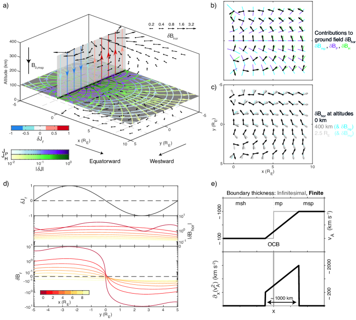
The model used typical dayside field line lengths of , ionospheric conductances valid for sunlit high-latitude regions, and zero magnetic shear across the magnetopause. We present results for one example surface mode, a localised perturbation with wavelength of along the field (fundamental mode) and azimuthally, based on previous simulation results (A21; M\BPBIO. Archer \BOthers., \APACyear2022, hereafter A22). This is applied to a single time, shown in Figure 1a, since the entire pattern will propagate along . The model size is twice the dimensions of that shown, to mitigate potential edge effects.
Figure 1a shows the Pedersen currents (purple) provide current closure in the East-West direction for the FACs. This is unlike in FLRs where closure is typically North-South (e.g. Greenwald \BBA Walker, \APACyear1980). While the Pedersen currents are strongest along the OCB, due to the finite conductivity they spread out significantly across the ionosphere too. Their magnitudes fall off with distance from the OCB, but extend well beyond the evanescent -folding scale of the magnetospheric signatures, given by . Pedersen current patterns result in Hall current vortices (green) surrounding the FAC sources/sinks at the OCB. Their sense of rotation is clockwise for downward FACs and anticlockwise for upward FACs. Hall current magnitudes decrease with distance identically to the Pedersen currents, due to the conductivities used. Since ionospheric velocities are given by the drift, Pedersen currents result in TCVs colocated with the Hall current vortices but with the opposite sense of rotation. As the background magnetic field is uniform in this model, convection speeds also fall off similarly with distance from the OCB.
We now focus on the directions of the horizontal magnetic field perturbations, shown in Figure 1a as black arrows above and below the ionosphere. The ground magnetic signals exhibit a vortical pattern centred at the midpoint of the FACs. Figure 1b shows the relative contributions of different current systems (colours) to the overall horizontal field (black). This reveals the field points mainly in the direction of the Hall current contribution, with magnetopause and Pedersen current magnetic fields largely opposing one another. In the case of an infinite plane Alfvén wave (for vertical background field and uniform conductances) the ground magnetic field is entirely dictated by Hall currents with FAC and Pedersen contributions cancelling (Hughes, \APACyear1974). However, we notice in Figure 1b that the total horizontal field is slightly misaligned from the Hall current contribution, due to magnetopause and Pedersen contributions no longer perfectly cancelling. This occurs because, in the case of a surface wave, while the largest contributions to the ground field from the Hall and Pedersen currents still arise from above the ground station, the FACs into the ionosphere are confined to the OCB and thus are generally not directly overhead. This results in the misalignment growing with distance from the OCB, as well as very close to the OCB but on the outer edges of the localised FACs, as can be seen in Figure 1b.
Figure 1a shows that the horizontal field perturbations above and below the ionosphere are rotated from one another, seemingly by right angles. While an exactly rotation would be expected for a plane Alfvén wave here (Hughes \BBA Southwood, \APACyear1974; Hughes, \APACyear1974), Kivelson \BBA Southwood (\APACyear1988) suggested that no rotation in the field might occur sufficiently far from a surface wave. We find this not to be the case for up to the -folding lengths shown. Panel c compares the directions of the ground field (black) to those at two altitudes above the ionosphere (greys). From these it is clear this rotation is not and that the rotation angle also depends on altitude. This is because ionospheric Pedersen and Hall currents contribute to the magnetic field above the ionosphere, as evidenced by the blue lines which show only the field due to magnetopause currents (less sensitive to altitude). The difference between the grey and blue arrows grow with distance from the OCB, for similar reasons as to which current systems are closest. Such an effect would be less prominent with a plane Alfvén wave since FACs permeate space above the ionosphere. Above the ionosphere, the direction of the magnetic field due to only magnetopause currents are much closer to different from the ground than the total field. The discrepancy from a right angle is exactly that due to the non-cancellation of magnetopause and Pedersen currents on the ground shown in panel b. This discrepancy will vary quantitatively with ionospheric conductivity and surface mode wavelength.
We now consider both horizontal and vertical components of the ground magnetic field. The horizontal field magnitudes shown in Figure 1d clearly show an overall decreasing trend with distance from the OCB (colours). The vertical component has the same sense as the FACs into the ionosphere, i.e. reversing direction at . The vertical component’s magnitude also decreases with distance from the OCB. Close to the OCB the vertical component has root mean squared (RMS) values up to times larger than the horizontal component. However, its RMS drops off much more quickly with distance, with them becoming equal at (), hence is largely negligible at further distances. The horizontal and total magnetic field magnitudes on the ground have RMS values and those of the incident/reflected waves, i.e. only including the magnetopause currents (when all current systems are considered above the ionosphere the ratios become ). Thus despite infinitesimal latitudinal width of FACs, the ionosphere might not screen the surface mode from the ground as suggested by Kivelson \BBA Southwood (\APACyear1988). The ionospheric screening effect goes as , where is the ionospheric altitude, meaning that the small latitudinal wavenumbers are not suppressed. While in the -direction there is only one wavenumber present, in the -direction the delta function in the current has equal Fourier amplitudes at all wavenumbers, thus small total wavenumbers in this superposition may be transmitted to the ground. This highlights the need when applying the Hughes \BBA Southwood (\APACyear1976) formulae for non-plane waves to use Fourier (or spherical harmonic) decomposition, rather than simply measures of spatial amplitude extent (cf. Ozeke \BOthers., \APACyear2009).
Finally, we quantify the extent to which each current system controls the total ground magnetic field through computing the Coefficient of Determination (see A). Since the pattern propagates, integration in time is equivalent to spatially along . This is performed at each distance away from the OCB. On average the Hall currents explain of the variance in the ground field across all components (further statistics are given in Table S1), hence they still exhibit overwhelming control within the model.
We find that changing wavelengths and ionospheric conductivities in this model lead to qualitatively similar results, but leave a full parameterisation to future work. However, we briefly discuss the likely effect of introducing a finite boundary thickness, which will change the surface magnetopause currents used into volume currents. Figure 1e considers a linear Alfvén speed variation between the two half-spaces (black) as in Chen \BBA Hasegawa (\APACyear1974), comparing this to the infinitesimal boundary used thus far (grey). Southwood \BBA Kivelson (\APACyear1990) note that in an azimuthally-uniform box model, FAC sources in a cold plasma are proportional to the product of: (1) the gradient in squared Alfvén speed; and (2) azimuthal derivative of the compressional magnetic field signal. The figure shows while in the infinitesimal case term (1) is non-zero coincident with the OCB, for a finite thickness boundary term (1) instead peaks at the inner edge of the magnetopause layer due to the high magnetospheric Alfvén speed. This is no longer coincident with the OCB, which will be located somewhere within the boundary. Considering term (2), outside of the boundary layer the surface mode’s compressions must decay exponentially with distance from the magnetopause within the two half-spaces. The sign of the compressions must also reverse within the boundary layer itself. These two facts necessitate that term (2) exhibit peaks near the boundary layer edges (see also Figure 1 of A22). Combining both terms suggests surface mode FACs are largest near the inner edge of the magnetopause. This conclusion holds within a box model for more complicated transitions or if thermal effects are included (Itonaga \BOthers., \APACyear2000).
3 Global Simulation
We now employ a global coupled MI simulation to better understand magnetopause surface modes’ potential auroral, ionospheric, and ground magnetic signatures within a more representative environment.
3.1 Overview
The Space Weather Modeling Framework (SWMF; Tóth \BOthers., \APACyear2005, \APACyear2012) is used on NASA’s Community Coordinated Modeling Center (CCMC). This includes BATS-R-US (Block-Adaptive-Tree-Solarwind-Roe-Upwind-Scheme; Powell \BOthers., \APACyear1999) global MHD magnetosphere, which is run at high-resolution ( in the regions considered), coupled to an electrostatic thin-shell ionosphere (Ridley \BOthers., \APACyear2004), where the same uniform conductances as in section 2 are used. The run, which was previously presented by A21 and A22 (based on H15), simulates the magnetospheric response to an idealised solar wind pressure pulse under northward IMF. Full setup details are in Table S2.
Here we summarise salient results from the BATS-R-US simulation. H15 showed, following an initial transient response, the pulse excites damped monochromatic compressional waves near-globally with frequency. Amplitudes of these waves decay with distance from the magnetopause, with a phase reversal across the boundary. The authors concluded these oscillations could only be explained by MSE. A21 found that across most of the dayside, magnetopause displacements showed little azimuthal phase variation. Indeed, the surface waves are stationary between Magnetic Local Time (MLT), despite non-negligible magnetosheath flows being present. They demonstrated this is achieved by the time-averaged Poynting flux inside the magnetosphere surprisingly pointing towards the subsolar point, balancing advection by the magnetosheath flow such that the total wave energy flux is zero. Outside of this region, waves are seeded tailward at the dayside natural frequency and grow due to KHI. A22 reported the magnetospheric velocity polarisation’s handedness in the stationary region (Earthward of the surface mode’s turning point) was also reversed from that typically expected, which was found only in the tailward propagating regions. While associated magnetic field polarisations can be reversed by the field geometry near the cusp, Earthward of each field line’s apex both polarisations are the same. A consequence of these results is MSE must have spatially varying wavenumbers. Across the dayside the system response is large-scale () and thus insensitive to the flow. Since fluctuations seeded downtail from the dayside have fixed frequency in Earth’s frame, in the flanks this results in the Doppler effect (i.e. due to the significant flow velocities) imposing shorter wavelengths along the magnetopause of . Normal to the magnetopause, phase fronts inside the dayside magnetosphere slowly propagate towards the boundary (). The authors argued this results from the magnetosonic dispersion relation (equation 1) when both compressibility and damping of the surface wave are taken into account. Finally, the surface mode is shown to couple to MHD body waves where their eigenfrequencies match: waveguides were found along the equatorial terminator () and outer nightside flanks; FLRs were identified on the equatorial terminator Earthward of the magnetopause and in the magnetotail (A21; A22).
As in those previous studies, in this paper we focus on the MSE response (times ) neglecting the directly-driven transient activity. Perturbations (represented by ’s) from equilibrium (represented by subscript ’s) are extracted by subtracting LOESS (locally estimated scatterplot smoothing; Cleveland, \APACyear1979) filtered data, where outliers were neglected. This removed long-term trends well during the period of interest, with spurious values occurring only before the arrival of the pulse. For the ionosphere and ground, coordinates employ Northward and Eastward horizontal components as well as the vertical/radial direction. In the magnetosphere, an equivalent field-aligned system is used. The field-aligned direction is the time-average of the LOESS-filtered magnetic field. Other directions are obtained as perpendicular projections of the local spherical polar unit vectors ( for colatitude and for azimuth). Specifically, the perpendicular Northward direction is and perpendicular Eastward is . All Fourier analysis is computed between and limited to frequencies , with results being integrated over this band.
3.2 Validity
We must assess the validity of using this simulation to qualitatively predict auroral, ionospheric, and ground magnetic signatures of magnetopause surface modes. We do not aim for fully quantitative predictions due to known limitations of current global MHD codes, such as numerical diffusion and current sheet smearing which underestimate ULF wave effects (S. Claudepierre \BOthers., \APACyear2009; H15). Thus only trends in wave patterns should be interpreted, rather than absolute amplitudes of signatures.
Global MHD models are not able to simulate down to ionospheric altitudes, e.g. since high Alfvén speeds slow down computations, thus magnetospheric boundary conditions are imposed on the plasma and fields further out ( here). This leaves a gap region between the magnetosphere inner boundary and the thin-shell ionosphere ( altitude) which is not simulated, as depicted in Figure 5a. MI-coupling occurs a few grid cells radial of the magnetosphere inner boundary (), where FACs are mapped and scaled through the gap region to the ionosphere along dipole field lines (Ridley \BOthers., \APACyear2004). This means equatorward of magnetic latitides there are no gap region FACs, hence we limit all analysis to poleward of . The ionosphere model solves for the electric potential via current continuity with a given conductance pattern, similarly to section 2, which yields ionospheric electric fields, currents, and velocities. The potential is mapped back to the magnetospheric inner boundary, setting the electric field and velocity there also.
As highlighted by Kivelson \BBA Southwood (\APACyear1988) and indicated in Figure 5a, compressional and shear MHD waves will affect the ionosphere differently due to their different currents. Shear modes exhibit FACs, hence coupling between the magnetosphere and ionosphere will occur, which in simulations will be performed by the current mapping. In contrast, compressional modes have only perpendicular currents and so no current is expected to flow between the magnetosphere and ionosphere. Purely compressional waves result in no significant ionospheric effects, which will be true in simulations also. Therefore, the ionospheric response to incident ULF waves should be reliable.
Potential issues, however, arise when considering ground magnetic field calculations. These are computed by Biot-Savart integration of all current systems: ionospheric Pedersen and Hall currents; those throughout the magnetosphere domain; and gap region FACs (Yu \BOthers., \APACyear2010; Rastätter \BOthers., \APACyear2014). Because the MI-interface in simulations is much further away than in reality, perpendicular currents at this interface will make much smaller contributions than they would otherwise due to the increased distance. FACs, on the other hand, are unaffected as they can traverse the gap region. This is illustrated in Figure 5a and could affect both types of MHD waves, though likely more acutely for compressional modes.
We first investigate the amplitudes of compressional and shear modes via the curl and divergence of the electric field perturbations as before. Due to available model outputs on the CCMC, these are calculated via
| (6) |
for the compressional mode, and
| (7) |
for the shear mode, where is the vorticity. Figure 5b–d shows Fourier wave amplitudes, along with their ratio, for a near-equatorial plane (). At the magnetopause, the OCB is shown as the black solid line and the magnetopause inner edge as the dashed line, which has been manually identified based on the background current, Alfvén speed, and velocity polarisation (A22) and fitted to a polynomial with local time. The large (e.g. at noon) boundary width in the simulation is a consequence of MHD being unable to resolve small gyroradius scales that dictate the thickness of the real magnetopause (Berchem \BBA Russell, \APACyear1982). Panel b demonstrates compressional mode amplitudes are generally largest near the magnetopause and decay slowly across the magnetosphere with distance from the boundary. Panel c shows shear wave amplitudes exhibit strong peaks inside the boundary layer, consistent with Plaschke \BBA Glassmeier (\APACyear2011), both at the inner edge and OCB. Away from these peaks, the amplitude falls off much more quickly than in the compressional mode. However, shear amplitudes remain larger than compressional ones almost throughout the equatorial magnetosphere, as indicated by the ratios in panel d. Since dayside FLR frequencies in the simulation are much larger than the observed waves (A22), we conclude the large shear amplitudes are due to non-resonant coupling between the compressional and shear modes. This occurs due to the inhomogeneous Alfvén speed and curvlinear magnetic geometry present (e.g. Radoski, \APACyear1971), resulting in a single wave that has mixed properties of both. The same quantities are also shown at , near the simulation MI-interface, in Figure 5e–g, where these have been projected along dipole field lines to the northern hemisphere ground. The OCB is found to occupy a small area around the displayed black dot, indicating a mostly closed magnetosphere as has been seen in extended northward IMF simulations previously (Song \BOthers., \APACyear2000; Zhang \BOthers., \APACyear2009). The magnetopause inner edge maps to latitudes equatorward of the OCB. Compressional mode amplitudes (panel e) are significantly weaker near the MI-interface, in agreement with the expected standing structure (Plaschke \BBA Glassmeier, \APACyear2011). They appear constrained to regions equatorward of the magnetopause inner edge and mostly to the dayside. Shear mode amplitudes (panel f) exhibit strong ridges on both flanks which are well-aligned with the inner/equatorward edge of the magnetopause, along which the amplitudes grow with MLT away from noon. Isolated peaks also occur equatorward of the inner edge on the terminator, corresponding to the FLRs identified by A21. Notably no clear peak occurs at the OCB. At the ratio of the shear to compressional mode amplitudes are even greater than at (panel g), indicating again the mixed properties of the wave.
The dominance of shear wave amplitudes over compressive suggests simulation results should be reliable. However, it is currents which are more crucial. Therefore, panels h–m display Fourier amplitudes for the perpendicular and parallel currents (and their ratios) at the same locations. Reassuringly the two components have similar patterns to the two wave modes. In particular, at FACs peak along the magnetopause inner/equatorward edge and at the discrete FLRs. No such peaks are present at the OCB, despite these occuring out in the magnetosphere. While at perpendicular and parallel currents are generally of similar magnitude, at the MI-interface FACs dominate poleward of latitudes (though the current ratio is not as large as that for mode amplitudes). Consequently, as perpendicular currents are small compared to FACs where MI-coupling is performed, Biot-Savart integration will be reliable in estimating ground magnetic field signals at high latitudes.
3.3 Optical aurora
FACs associated with FLR can result in periodic optical auroral forms (Greenwald \BBA Walker, \APACyear1980; Samson \BOthers., \APACyear1996; Milan \BOthers., \APACyear2001). Upward FACs at the ionosphere are carried by precipitating electrons that may, if sufficiently energetic, cause auroral emission, whereas regions of downward FACs appear relatively darker. Given we have demonstrated surface modes also exhibit FACs, it is worth exploring their potential auroral signatures.
As shown in panels i and l of Figure 5, oscillatory FACs associated with the surface mode peak at the inner edge of the magnetopause rather than the OCB. This is difficult to intuit theoretically within a realistic magnetosphere (Southwood \BBA Kivelson, \APACyear1991; Itonaga \BOthers., \APACyear2000), especially since the simplifying assumption of wave scales being smaller than changes in background conditions cannot be made (A22). Nonetheless, the result is in agreement with the box model prediction of section 2. Movie S1 (left) shows perpendicular velocity perturbations near the magnetospheric equator. While near the subsolar point motion is largely normal to the boundary, away from the Sun-Earth line vortical structure emerges near the magnetopause, particularly at the flanks. The clearest structures have vortex cores Earthward of the OCB, corresponding to the inner surface mode (Lee \BOthers., \APACyear1981; A22). These are associated with significant field-aligned vorticity, though this quantity is prevalent throughout the magnetosphere (middle). In a uniform plasma only Alfvén waves exhibit parallel vorticity, hence this results from non-resonant coupling between the compressional and shear modes. On the dayside magnetosphere, the vorticity’s phase structure has shorter normal scales () than transverse ones (the entire morning/afternoon sector). There is also slow () phase motion towards the boundary. Since all signals’ amplitudes decay with distance from the magnetopause inner edge, the vorticity appears to grow as its phase fronts travel towards the boundary. These features are very similar to those reported in A21 for the compressional magnetic field, explained as the result of surface wave damping. We also note these boundary normal wavelengths are much larger than those expected for field line resonance, since the large gradients in FLR frequencies (A22) suggest scales (Southwood \BBA Allan, \APACyear1987). In contrast to the dayside, tailward of approximately the terminator, transverse wavelengths shorten to and phase motion appears predominantly tailward. Vorticity magnitudes in the flanks are significantly larger than on the dayside due to KHI-amplification and the shorter scales. We note that coupling of MSE to body modes, such as waveguides or FLR, has been shown to occur in these regions (A21), hence results in the nightside magnetosphere are generally a superposition of wave modes (including surface waves). Finally, FAC patterns (right) are very similar to the vorticity, as expected theoretically by Southwood \BBA Kivelson (\APACyear1991). Thus, magnetopause surface modes may exhibit FACs not just within the boundary, as in simple box models, but throughout the magnetosphere.
Based on these results near the equatorial plane, we expect that FAC structures at the MI-interface due to the surface mode consist of large-scale (compared to those of Alfvén waves) poleward moving forms on the dayside. Indeed, this can be seen in Movie S2 (left) which shows the ionospheric FAC input. On the dayside, FAC latitudinal wavelengths are ( in the ionosphere), larger than expected for FLRs in this region ( or ). The structures propagate polewards at (or equivalently ), growing in amplitude with their phase motion until they peak at the projection of the magnetopause inner/equatorward edge (as demonstrated in Figure 5i). The azimuthal extent of these waves is likely a function of the driver, hence solar wind excited surface waves like in the simulation should exhibit more extended FACs than those due to most foreshock transients (Sibeck \BOthers., \APACyear1999) or magnetosheath jets (M\BPBIO. Archer \BOthers., \APACyear2019). In the simulation, we find that outside of the MLT stationary region FAC structures propagate principally towards the tail, forming periodic structure along the projection of the boundary’s inner/equatorward edge. While on the dayside structures appear azimuthally stationary, like the surface waves in the magnetosphere, the tailward propagating behaviour of the eigenmode outside the stationary region causes the FACs to bifurcate at the boundary between the two regimes during their poleward phase motion. This results in more complex structure than simply a (spherical) harmonic wave.
We conclude that magnetopause surface modes might have optical auroral signatures somewhat similar to FLRs. These consist of periodic brightenings with latitudinal arc widths of that propagate polewards at slow speeds of (). The intensity of these periodic aurorae should amplify with their phase motion, peaking not at the OCB as had been thought before (O. Kozyreva \BOthers., \APACyear2019), but equatorward of it at the projection of the magnetopause inner edge. In our simulation the OCB and magnetopause inner/equatorward edge are highly separated, about in latitude at noon. However, this is merely due to the large magnetopause thickness. We estimate realistic separations between the OCB and magnetopause inner/equatorward edge to be for the driving conditions considered. This is based on the latitudinal difference in the simulation of traced footpoint locations from field lines separated by the boundary widths reported by Berchem \BBA Russell (\APACyear1982). Thus dayside auroral brightenings associated with surface modes, when visible due to the time of day / season, might consist of poleward moving arcs that intensify towards and peak a few degrees equatorward of an OCB proxy. Further into the flanks, auroral brightenings may form clear periodic structure along the projection of the boundary inner/equatorward edge, which will principally propagate azimuthally. KHI will likely make these auroral features generally stronger on the flanks. The auroral signatures of surface modes might be distinguished from FLR by their higher latitude location, lower frequency, and larger latitudinal extent. However, we make no claims here on the character, colour, or taxonomy of such potential auroral signatures, since these cannot be easily predicted by MHD simulations. It also remains to be seen whether these auroral signals can be extracted from background emissions under different activity levels.
3.4 Ionospheric convection
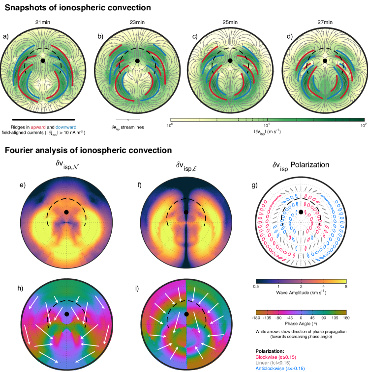
Perturbation convection patterns are shown in Figure 2a–d as streamline snapshots over approximately half a cycle, and in Movie S2 as animated quivers. These reveal on the dayside large-scale convection vortices are present, which circulate the FAC maxima (bold lines in Figure 2a–d). Vortices are clockwise for upward currents and anticlockwise for downward, in agreement with section 2. Interestingly, the vortex cores are located at and MLT, i.e. the transition between stationary and propagating magnetopause surface waves. Like the FACs, dayside vortices have shorter latitudinal scales than longitudinal. At the lower latitudes considered though, vortices appear more spread out in the equatorward direction. This is likely because successive FAC structures become weaker towards the equator, making the ionospheric response more like in the box model. Since dayside FAC structures move polewards and grow in strength towards the magnetopause inner/equatorward edge, the convection vortices travel polewards and exhibit increases in speed up to this point also. Thus poleward-moving sequences of TCVs on the dayside may be a clear ionospheric signature of MSE. These are unlike typically reported isolated / pairs of TCVs associated with the direct impacts of solar wind / foreshock pressure pulses or flux transfer events, which exhibit only tailward motion (Friis-Christensen \BOthers., \APACyear1988; Sibeck, \APACyear1990), suggesting this phase motion could be a potential diagnostic for identifying MSE in ground-based data.
Figure 2e–f shows Fourier amplitudes of the two ionospheric velocity components. Around noon signals are mostly North-South, like the radial motions exhibited in the magnetosphere in this sector (A21; A22). Amplitudes peak at the magnetopause inner/equatorward edge, just like the FACs. However, the amplitude of the East-West component increases significantly away from noon towards the flanks. This is most evident in panel g, which displays polarisation ellipses derived from the Fourier transforms (as outlined in A22). Away from noon the ellipses’ orientations rotate away from the North-South direction and the magnitude of their ellipticity increases. Ionospheric velocity polarisations show consistent handedness with those out in the equatorial magnetosphere (A22), in particular a reversal is present either side of the transition between stationary and propagating surface waves. Panels h–i indicate phases and propagation directions for the velocity components, which are quite different from one another. There is little phase variation in the North-South component on the dayside, with only slight poleward phase motion in the stationary region. This reflects the large-scale periodic North-South motion associated with the surface waves that is clear from Movie S2. In constrast, the East-West component exhibits much larger gradients in phase latitudinally across the dayside. These differences are due to a combination of the vortices’ larger longitudinal scales compared to latitudinal along with the poleward motion of these vortices. Azimuthal phase variation is introduced in the tailward propagating regime for both velocity components, though is clearest in the North-South direction.
The finite ionospheric conductivity causes significant spreading out of patterns caused by localised FACs. Therefore, in the above we have focused on the dayside as we know an FLR is also present at lower latitudes on the terminator. Figure 2e–f shows that at the terminator two amplitude peaks on each flank are present in both components. One of these is near the magnetopause inner boundary corresponding to the surface mode, whereas the lower latitude peak is due to the FLR. There is clearly significant spreading longitudinally of the FLR-related amplitude structures by , meaning that ionospheric convection patterns in general consist of a complex superposition of those due to the surface mode and its coupled FLR(s). Only within of noon is the ionospheric response dominated by the surface mode.
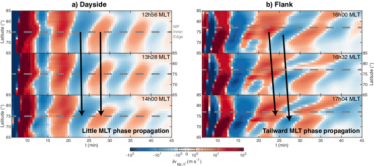
Figure 3 shows potential ionospheric Doppler radar observations, emulating typical range-time plots. These show the time variation of the North-South velocity perturbations with latitude for nearby local times. Figure 3a corresponds to the dayside, which clearly shows in each panel periodic oscillations in the ionospheric velocity that exhibit poleward phase motion and peak in amplitude near the projection of the magnetopause inner boundary (grey dashed line). Comparing the panels indicates there is little phase propagation in MLT since the surface waves are stationary, again unlike typical tailward TCVs. Figure 3b corresponds to the flanks, highlighting the increased complexity of the signal away from noon. Nonetheless, some similar features to the dayside are seen. While the amplitude does maximise near the magnetopause inner boundary due to the surface mode, a secondary amplitude maximum is present at lower latitude associated with the terminator FLR. All of these patterns in the flank exhibit tailward phase propagation when comparing panels.
3.5 Ground magnetic field
Ground magnetic field perturbations were computed using the CalcDeltaB post-processing tool (Rastätter \BOthers., \APACyear2014), performed in SM coordinates due to the idealised model setup. We compare these to the magnetic field signals near the MI-interface. Both are shown in Movie S3.
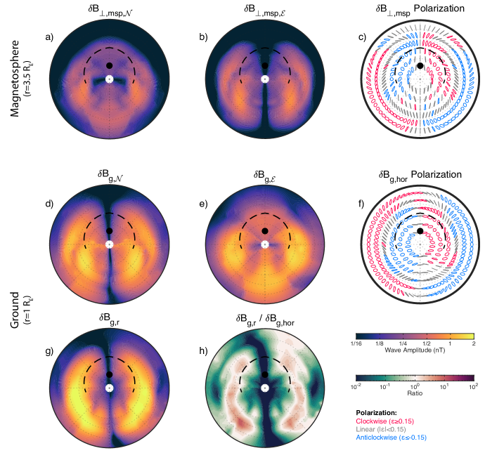
Figure 4a–c show the wave amplitudes and polarisations in the magnetosphere near the MI-interface. On the dayside perturbations are predominantly North-South oriented and maximise at the magnetopause inner/equatorward edge. In contrast, as shown in panels d–f, on the ground the magnetic field is mostly in the East-West direction. The movie shows these East-West signals are coherent across most of the dayside, converging/diverging from the ionospheric vortex cores at and MLT. This is unlike toroidal mode Alfvén waves, some of the most intensively studied ULF waves, which are aligned mostly North-South on the ground. The Fourier amplitude maps at the MSE frequency in Figure 4 for the ground horizontal components resemble those in the magnetosphere for the other component, i.e. that at right angles. Ground signals are of significantly greater amplitude than in the magnetosphere. While this is similar to the box model, in the simulation this will partly be due to the scaling of FACs across the gap region with . Ground magnetic field amplitudes also appear more extended than above the ionosphere. This is due to the spreading of currents in the ionosphere by the finite conductance, as discussed previously, as well as spatial integration of these ionospheric currents (Plaschke \BOthers., \APACyear2009). The handedness of wave polarisations above and below the ionosphere are largely the same. Notable differences occur at the lowest latitudes shown, where the ground magnetic field is less reliable. Generally we see the ground magnetic field has greater ellipticity than in the magnetosphere, likely due to finite ionospheric conductance spreading out the currents’ vortical patterns.
The time-averaged rotation angle from the magnetosphere to the ground was calculated for each point using the Fourier method outlined in B. Over the region depicted, this had a mean and standard deviation of . Note the magnetic field near the MI-interface does not include contributions from ionospheric Pedersen and Hall currents, hence is associated with the incident/reflected waves only. We find in agreement with the box model that the ionosphere rotates surface wave magnetic fields by close to , though significant spread in this angle occurs. Unlike in section 2, however, we found no systematic spatial ordering of the rotation angle. This may be because in the simulation FACs are not confined to within the boundary and move poleward. We again compute the Coefficient of Determination at each point to quantify the contribution of different current systems to the total ground magnetic field. Here this is done using Fourier methods, as outlined in A. As in the box model, it is Hall currents which dominate the ground field, hence why the rotation angle is close to . However, on average Hall currents explain only of the variance across all components – much smaller than in the simple box model. Tabel S1 demonstrates, however, that the other current systems (excluding Hall) and their combinations are not significant predictors of the ground field. Therefore, the total variance on the ground must be a complex superposition of many current systems, including most notably Hall currents.
Movie S3 also shows the vertical component of the ground magnetic field. Qualitatively this somewhat resembles the FACs, in line with predictions from the box model. However, Figure 4g shows towards the flanks, unlike the FACs, the vertical field amplitudes peak at lower latitudes than the magnetopause inner/equatorward boundary. At the terminator the peak corresponds well with the FLRs. Therefore, it appears that the FLR is dominating the vertical field perturbations on the ground, relative to surface mode, across a wide local time range. Vertical field amplitudes are generally greater than the horizontal ones only in the vicinity of their peaks. Close to noon, however, the vertical field is weak and only becomes significant at and MLT, the locations of dayside ionospheric vortex cores. Thus, like with the ionosphere, only in the vicinity of noon are the ground magnetic perturbations solely due to the surface mode.
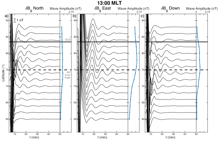
Figure 5 shows stacked time-series of a latitudinal chain of virtual ground magnetometers located close to noon, where effects of the FLR are small. These demonstrate poleward phase motion of the ground magnetic field in all three components, unlike ground magnetometer observations of typical isolated / pairs of TCVs which show predominantly tailward motion (e.g. Friis-Christensen \BOthers., \APACyear1988). Like with the ionospheric velocity though, this phase motion is slightly different for all three components. The amplitude variation (blue lines) is quite broad for all three components. While the vertical component appears to peak at the magnetopause inner/equatorward edge, the East-West component’s maximum appears shifted slightly poleward of this location and the North-South component has a rather flat peak. Nonetheless, all three maxima are clearly closer to the magnetopause inner/equatorward edge than the OCB within the simulation. We suggest that all these features could be used as diagnostics for identifying surface modes in ground magnetometer networks.
4 Discussion
4.1 Limitations
In both aspects of this study we have employed uniform ionospheric conductances. This was to understand the surface mode’s ground-based signatures in the simplest case. Improved empirical conductance maps typically include effects of solar illumination and/or auroral oval conductance contributions (Ridley \BOthers., \APACyear2004). The former exhibit relatively small variations over scales much larger than surface mode wavelengths, hence likely have little effect on the predictions. In contrast, auroral oval Hall conductances can be significantly larger than those outside this region. While these could result in stronger currents within the auroral oval, and thus stronger ground magnetic signals, the sense of FAC closure would likely remain. Hartinger \BOthers. (\APACyear2017) performed simulations comparing ground field perturbations from a solar wind pressure increase under different conductance models. They found qualitatively similar results for the uniform and solar conductance patterns, but somewhat different amplitude profiles with the auroral pattern.
So far we have treated the ground as a perfect insulator, in line with most past global modelling and observational work (e.g. Samsanov \BOthers., \APACyear2015; Tanaka \BOthers., \APACyear2020). While some other ULF wave studies have considered the ground to be a perfect conductor (e.g. Hughes, \APACyear1974; Hughes \BBA Southwood, \APACyear1974; Waters \BBA Sciffer, \APACyear2008), neither regime realistically includes contributions from induced telluric currents in the ground. To estimate their likely effect we apply the Complex Image Method (Boteler \BBA Pirjola, \APACyear1998; Pirjola \BBA Viljanen, \APACyear1998). This places an image current, with the same strength as that in the overhead ionosphere, at a depth of for complex skin depth . Here we take this skin depth to be
| (8) |
where is the ground conductivity. One can assume a uniform conductivity that is able to capture the spatial variations in the field/currents through a plane wave (Pirjola \BOthers., \APACyear2009). For wavelengths and periods , valid for MSE, this yields values of , in line with ground conductivities for rocky or city areas (Cebik W4RNL, \APACyear2001). These values along with the simulation MSE frequency result in skin depths of magnitude , much greater than the ionospheric altitude. Given that in both the box model and simulation the ground magnetic field was mostly dictated by Hall currents with large scale sizes, we estimate the ground magnetic fields from telluric currents by assuming an infinite line current in the ionosphere (Boteler \BBA Pirjola, \APACyear1998). This predicts horizontal ground magnetic field perturbations are amplified by and vertical fields reduced by due to the induced ground currents. Phase changes are negligible (). These are relatively small contributions due to the low frequency of the surface mode, since lower frequencies are less effective at inducing telluric currents for a given amplitude. In contrast, higher frequency ULF waves of are predicted to change the horizontal field by . We also note that near oceans, the high conductivity of salt water likely renders all ULF waves’ ground signatures greatly affected (). Future studies could more comprehensively investigate the importance of telluric currents to ground magnetometer signals of surface and other ULF waves.
Our brief evaluation of these limitations suggests the use of a wide range of latitudes when examining potential observations to these predictions, where overall trends likely persist. On smaller scales, local effects due to varying conditions in the ionosphere and the ground may be more important, which could form the basis of future work.
4.2 Comparison to previous observations
Auroral brightenings, ionospheric convection vortices, and ground pulsations are expected from FACs in general. However, mapping observations from the ground out to space is difficult when trying to distinguish surface waves from nearby body waves. We thus limit comparitive discussion to studies that could better constrain ground-based observations.
Previous conjugate observations have linked aurorae to surface waves. He \BOthers. (\APACyear2020) suggested sawtooth aurorae, large-scale undulations along the equatorward edge of the diffuse aurora, may be the optical atmospheric manifestation of plasmapause surface waves. During a geomagnetic storm, they showed plasmapause surface waves (i.e. with similar frequencies to MSE) in the afternoon-dusk correlated with sawtooth auroral patterns near the footpoints of the plasmapause field lines, with wavelengths and propagation speeds of both being in agreement. The authors suggested the modulation of hot plasma by the plasmapause surface mode may have led to particle precipitation, and thus diffuse aurora. Similarly, Horvath \BBA Lovell (\APACyear2021) presented two case studies of KHI-waves on the flank magnetopause during geomagnetic storms, which appeared to excite surface waves on / near the plasmapause in the hot zone of the outer plasmasphere. During these events, correlated complicated sub-auroral plasma flows and large auroral undulations were observed at low Earth orbit. The authors conclude magnetopause surface modes couple, in complex ways, to the inner magnetosphere and auroral zones. Finally, the ground-based study of O. Kozyreva \BOthers. (\APACyear2019) used observations of the equatorward edge of the red cusp aurora as an optical proxy for the OCB following southward IMF turnings. They noted quasi-periodic motion of this boundary in 3 events, which they interpreted as evidence for MSE. While these studies demonstrate a connection between magnetopause/plasmapause surface waves and aurorae, the latter’s generation mechanism remains unclear. Further work should determine whether surface waves’ FACs directly result in periodic aurorae or merely perturb existing auroral current systems.
M\BPBIO. Archer \BOthers. (\APACyear2019) first showed MSE signatures may be present in dayside ground magnetometer data, though unfortunately data was low resolution and had poor spatial coverage which limited conclusions. O. Kozyreva \BOthers. (\APACyear2019) presented data from a near-noon latitudinal chain following impulsive external driving. Short-lived oscillations in the North-South component were found to peak equatorward of the optical OCB proxy. While the authors attributed this to experimental uncertainty, it is unclear why this would result in a systematic effect. The offset agrees with our estimates for the inner/equatorward edge of the magnetopause boundary layer, thus could instead be consistent with our results. They also noted poleward phase motion and large latitudinal scales, both like in our simulation. He \BOthers. (\APACyear2020) demonstrated ground magnetic pulsations associated with plasmapause surface waves in the afternoon-dusk sector. A latitudinal magnetometer chain showed clear poleward phase motion, as in the simulation. However, the authors suggest the plasmapause surface wave may have coupled to an FLR outside the plasmasphere due to the amplitude and phase structure observed, potentially complicating these observations. Finally, Hwang \BOthers. (\APACyear2022) presented two case studies of KHI-waves and their ground effects. Vortical horizontal field perturbations were observed at high latitudes, corresponding to bead-like FACs elongated in the east-west direction like those seen in the simulation flanks.
There are some interesting similarities and differences between these magnetopause surface mode results and the classic Sudden Commencement (SC) or, more generally, TCV response of the magnetosphere. These models are generally used to interpret ground-based observations following impulsive solar wind driving, e.g. interplanetary shocks or solar wind pressure pulses, hence warrant further discussion. The Araki (\APACyear1994) model of SC predicts bipolar variations of the geomagnetic field at polar latitudes due to a global ionospheric twin vortex resulting from pairs of FACs on each of the morning and afternoon sectors. These are similar but larger in scale than typical TCVs. Our simulation results are broadly consistent with this model during the transient period (see Movie S2 and Figure 6). The Araki (\APACyear1994) model, however, does not predict the subsequent periodic oscillations following this transient, which are associated with MSE. This is because it only considers the intensification of magnetopause currents and FACs related to a single ripple on the magnetopause, hence not a surface wave or eigenmode. This is also true of similar TCVs models (e.g. Sibeck, \APACyear1990). MHD wave propagation during SC is typically linked to the Tamao (\APACyear1964\APACexlab\BCnt1, \APACyear1964\APACexlab\BCnt2) path or cavity/waveguide theory (Kivelson. \BOthers., \APACyear1984; Kivelson \BBA Southwood, \APACyear1985), where compressional waves couple to FLRs at the location their (eigen)frequencies match. Thus the possible contributions of magnetopause surface waves has not been considered in past SC observations or modelling (see the review of Fujita, \APACyear2019). SC can often be followed by long period waves (e.g. Matsushita, \APACyear1962), however, these are rarely discussed. It is therefore possible that ground-based evidence of MSE could be prevalent in past SC observations, with the subsequent pulsations either being neglected or misidentified as cavity/waveguide modes and FLR, which are generally not expected to occupy such low frequencies on the dayside (M\BPBIO. Archer \BOthers., \APACyear2015).
Overall, our simulation results appear consistent with the few previous reported observational signatures of magnetopause surface waves specifically. However, some aspects could not be tested with the data presented, motivating the need for both dedicated future observational studies and reanalysis of previously examined events in light of this work.
4.3 Implications
The results presented in this paper have potential consequences within the context of space weather, which we briefly comment on.
We have demonstrated magnetopause surface modes are predicted to result in ionospheric currents and electric fields. This offers the possibility that surface wave energy may be dissipated in the ionosphere, like it is for other ULF wave modes (e.g. Glassmeier \BOthers., \APACyear1984). Joule heating rates are given by
| (9) |
where the first term corresponds to the DC equilibrium heating rate and the subsequent terms are associated with pulsations. Recall a uniform Pedersen conductance of was used, which is reasonable for sunlit high-latitude regions (cf. Ridley \BOthers., \APACyear2004). In the simulation, we integrate these over the entire dayside ionosphere. While the DC rate is , we find the maximum pulsation-related rate is , occurring during the transient response. The peak dissipation rate during times of confirmed MSE () is also significant compared to the background at (i.e. 13%). While the inclusion of the KHI-amplification of the surface waves and their coupling to FLRs on the nightside result in the global ionospheric dissipation rates being even greater during MSE times at 25% of the global DC rate, the ionospheric conductances in the nightside hemisphere are less realistic. Overall, these simulation results qualitatively suggest magnetopause surface modes may provide important contributions to ionospheric heating. Further work could quantitatively predict heating rates due to surface waves using a range of more representative wave amplitudes and ionospheric conditions, improving our understanding of their global significance under different driving regimes.
We also predict that magnetopause surface modes result in oscillatory magnetic fields at Earth’s surface. This suggests they could be a source of geomagnetically induced currents driven by geoelectric fields (e.g. Belakhovsky \BOthers., \APACyear2019; Heyns \BOthers., \APACyear2021). While geoelectric fields are frequency-dependent with a higher frequency bias relative to the underlying disturbance geomagnetic field (e.g. Boteler \BBA Pirjola, \APACyear1998; Pirjola \BBA Viljanen, \APACyear1998), distinct Pc5-6 frequency ULF waves () can result in significant measured geoelectric fields (Hartinger \BOthers., \APACyear2020; Shi \BOthers., \APACyear2022). Therefore, it may be possible that magnetopause surface waves, at either MSE or higher (e.g. intrinsic KHI) frequencies, could similarly result in strong geoelectric fields. Modelling this is beyond the scope of this study, as it is known the three-dimensional conductivity structure of Earth is important in accurate characterisation of geoelectric fields (Bedrosian \BBA Love, \APACyear2015). Therefore, further study is warranted in assessing whether magnetopause surface modes of more realistic amplitudes may be a source of geoelectric fields and thus geomagnetically induced currents (cf. Belakhovsky \BOthers., \APACyear2019; Heyns \BOthers., \APACyear2021; Yagova \BOthers., \APACyear2021).
5 Conclusions
We have investigated magnetopause surface waves’ direct effects on the aurorae, ionosphere, and ground magnetic field through both MHD theory and a global MI-coupling simulation. Our main conclusions are as follows:
-
1.
Magnetopause surface modes have associated FACs into / out of the ionosphere, which for a finite thickness boundary maximise at the inner/equatorward edge of the magnetopause rather than the OCB. Non-resonant coupling between the compressional and Alfvén modes results in further monochromatic FACs throughout the magnetosphere, hence are unrelated to the Alfvén continuum. The amplitudes of these currents fall off with distance from the magnetopause.
-
2.
The normal phase structure reported by A21 in the equatorial magnetosphere due to damping also manifests at the MI-interface as slow poleward moving FAC structures. With latitudinal wavelengths of on the dayside, these are large-scale compared to expectations for FLR.
-
3.
FACs associated with global MSE are weakest on the dayside, due to smaller boundary displacements and azimuthal scales that span the morning/afternoon sector. In the flanks, where the Doppler effect imposes shorter scales and wave perturbations are amplified through KHI, strong periodic FACs may be present along the magnetopause inner/equatorward edge.
-
4.
We suggest upward FACs associated with surface modes may lead to periodic auroral brightenings that peak in intensity at the magnetopause inner/equatorward edge. On the dayside, these auroral forms move slowly poleward at () and occupy large latitudinal bands compared to narrower FLR-related aurorae. Periodic longitudinal structure will reflect that out at the magnetopause..
-
5.
Ionospheric convection vortices circulate the surface mode’s FAC structures. Like the FACs, they are large-scale, poleward moving, and strongest at the magnetopause inner/equatorward edge. The finite conductivity causes ionospheric signals to be more spread out than the FACs.
-
6.
Magnetopause surface modes can also cause ground magnetic field signals. These are largely caused by Hall current vortices, which rotate the magnetic field perturbations from above the ionosphere to the ground by almost (though significant non-systematic spread in this rotation angle occurs). Therefore, ground signatures of MSE near noon are strongest in the East-West direction. Oscillations have the same frequency across -shells, amplitudes peak near the magnetopause inner/equatorward edge, and latitudinal variations are large-scale.
These conclusions provide qualitative predictions for magnetopause surface modes which might be applied to interpreting high-latitude ground-based data
Different plasma conditions throughout geospace are expected to slightly modify some of the features observed. Penetration of surface modes into the magnetosphere is governed by local normal wavenumbers (equation 1). This is very weakly dependent on the Alfvén speed distribution for MSE, due to its such low frequencies compared to FLR, thus varying the simulation inner boundary density or including a ring current would have little effect. The inclusion of a plasmasphere (S\BPBIG. Claudepierre \BOthers., \APACyear2016), however, might have a greater influence since it could lower the Alfvén continuum at the plasmapause to MSE-range frequencies. This would limit the surface mode’s access to the inner magnetosphere and lead to coupling to plasmapause surface waves and/or FLR on the dayside, introducing an additional superposition of waves. Nonetheless, surface mode signatures in the outer magnetosphere would be little affected. Different Alfvén speed distributions would, however, change the eigenfrequencies of WMs and FLRs, hence where MSE may excite these secondary waves. The polar cap in the simulation presented is very small. While our results (both theoretically and in the simulation) suggest surface mode currents at the MI-interface maximise at the inner/equatorward edge of the magnetopause boundary rather than the OCB, whether the amount of open flux affects possible currents near the OCB should be explored in future work. We also note this simulation is North-South and dawn-dusk symmetric due to zero dipole tilt, whereas interhemispheric (e.g. Engebretson \BOthers., \APACyear2020; Xu \BOthers., \APACyear2020) and dawn-dusk (e.g. Henry \BOthers., \APACyear2017) asymmetries in geospace are of great interest in understanding solar wind – magnetosphere – ionosphere coupling. Overall, how magnetopause surface modes manifest in the magnetosphere, ionosphere, and on the ground under varying magnetospheric conditions should be ascertained through series of further simulations.
Finally, a further potential avenue for remote sensing magnetopause (or even plasmapause) surface modes could be ionospheric Total Electron Content (TEC) data derived from Global Navigation Satellite Systems. Recent work has shown that ULF waves may modulate TEC, yielding periodic oscillations of similar frequency (V. Pilipenko \BOthers., \APACyear2014; Watson \BOthers., \APACyear2015; Belakhovsky \BOthers., \APACyear2016; O\BPBIV. Kozyreva \BOthers., \APACyear2020; Zhai \BOthers., \APACyear2021). While several mechanisms for this have been proposed, overall they remain poorly understood. Future work could use the predicted ionospheric electric fields associated with surface modes to drive height-resolved ionosphere and neutral atmosphere models (Ozturk \BOthers., \APACyear2020). This would crucially unveil how the coupled ionosphere – thermosphere – mesosphere system reacts to boundary waves in our magnetosphere.
![[Uncaptioned image]](/html/2303.01138/assets/x2.png)
(a) Illustration of magnetosphere–ionosphere coupling within global MHD simulations applied to compressional and shear ULF waves. (b–m) Simulation Fourier maps taken from the near-equatorial plane (b–d,h–j) and at near the simulation magnetosphere-ionosphere interface (e–g,k–m), the latter have been projected onto the ground. These show amplitudes of compressional (b,e) and shear (c,f) waves and associated currents perpendicular (h,k) and parallel (i,l) to the background magnetic field. Ratios are also shown (d,g,j,m). Solid black lines indicate the open–closed field line boundary whereas dashed lines indicate the magnetopause inner edge. Arrows highlight regions due to magnetopause surface eigenmode (MSE), waveguide mode (WM), and field line resonance (FLR).
Appendix A Coefficient of Determination
The Coefficient of Determination, , is the proportion of the variance in a dependent variable that is predictable from an independent variable, often used in statistical models to quantify how well outcomes are replicated. In the case that the variables are complex vector time-series, this is given by
| (10) |
where is the dependent variable and is its predicted/modelled value. It follows from Parseval’s theorem that for oscillatory signals can also be determined from the complex Fourier amplitudes (denoted by tildes here)
| (11) |
can be interpreted as the fraction of explained variance, with corresponding to perfect prediction. Negative values are possible when the predictor performs worse than one which always predicts the mean value. In this paper we use to indicate what proportion of the total ground magnetic field perturbations are determined by contributions from different current systems. This has the benefits over simply comparing the root-mean-squared magnitudes of contributions (e.g. Rastätter \BOthers., \APACyear2014) since the vector directions are also included.
Appendix B Rotation Angle
The signed right-handed rotation angle from a vector to about some direction may be expressed as
| (12) |
In the case of oscillatory vectors, the time-average (angular brackets) of can be arrived at by using the following properties of complex Fourier amplitudes
| (13) |
and hence
| (14) |
In this paper, we use this to calculate the rotation of the horizontal magnetic field components from above the ionosphere to below it. Thus the direction is taken as the vertical/radial.
Magnetosheath
Magnetopause
Magnetosphere
Ionosphere
Ground
Geocentric Solar Magnetospheric coordinates
Solar Magnetic coordinates
Northward component
Eastward component
Horizontal
Parallel to the magnetic field
Perpendicular to the magnetic field
Normal to boundary
Pedersen
Hall
Ellipticity
Vacuum permeability
Conductivity
Conductance
Electrostatic potential
Angular frequency
Vorticity
Magnetic field
Speed of sound
Electric field
Altitude
Current density
Wave vector
McIlwain field-line equatorial distance parameter
Geocentric Position
Field line length
Time
Plasma velocity
Alfvén speed
Open Research
Simulation results have been provided by the Community Coordinated Modeling Center (CCMC) at Goddard Space Flight Center using the SWMF and BATS-R-US tools developed at the University of Michigan’s Center for Space Environment Modeling (CSEM). This data is available at https://ccmc.gsfc.nasa.gov/results/viewrun.php?domain=GM&runnumber=Michael_Hartinger_061418_1 and https://ccmc.gsfc.nasa.gov/results/viewrun.php?domain=PP&runnumber=Martin_Archer_20211219_PP_1. Box model results generated are available in M. Archer \BOthers. (\APACyear2022).
Acknowledgements.
We acknowledge valuable discussions within the ISSI International Team project #546 “Magnetohydrodynamic Surface Waves at Earth’s Magnetosphere (and Beyond)”, led by MOA and Katariina Nykyri, thanks to support by the International Space Science Institute (ISSI) in Bern. MOA holds a UKRI (STFC / EPSRC) Stephen Hawking Fellowship EP/T01735X/1. MDH was supported by NASA grant 80NSSC19K0907 and NSF grant AGS 2027210. DJS was supported by STFC grant ST/S000364/1. MH was supported by NERC grant NE/V003070/1 and Schmidt Science Fellows, in partnership with the Rhodes Trust. JWBE was supported by NERC grants NE/P017142/1 and NE/V003070/1. A.N.W. was partially funded by STFC grant ST/N000609/1. XS is supported by NASA award 80NSSC21K1677 and NSF award AGS-1935110. For the purpose of open access, the author has applied a Creative Commons Attribution (CC BY) licence to any Author Accepted Manuscript version arising.References
- Araki (\APACyear1994) \APACinsertmetastarAraki1994{APACrefauthors}Araki, T. \APACrefYearMonthDay1994. \BBOQ\APACrefatitleSolar Wind Sources of Magnetospheric Ultra-Low-Frequency Waves Solar wind sources of magnetospheric ultra-low-frequency waves.\BBCQ \BIn M. Engebretson, K. Takahashi\BCBL \BBA M. Scholer (\BEDS), (\BPGS 183–200). \APACaddressPublisherWashington, DC, USAAmerican Geophysical Union. {APACrefDOI} 10.1029/GM081p0183 \PrintBackRefs\CurrentBib
- Araki \BBA Nagano (\APACyear1988) \APACinsertmetastarAraki1988{APACrefauthors}Araki, T.\BCBT \BBA Nagano, H. \APACrefYearMonthDay1988. \BBOQ\APACrefatitleGeomagnetic response to sudden expansions of the magnetosphere Geomagnetic response to sudden expansions of the magnetosphere.\BBCQ \APACjournalVolNumPagesJ. Geophys. Res. Space Physics933983–3988. {APACrefDOI} 10.1029/JA093iA05p03983 \PrintBackRefs\CurrentBib
- M. Archer \BOthers. (\APACyear2022) \APACinsertmetastararcher_data{APACrefauthors}Archer, M., Hartinger, M., Rastätter, L., Southwood, D., Heyns, M., Eggington, J.\BDBLShi, X. \APACrefYearMonthDay2022\APACmonth12. \APACrefbtitleMagnetopause Surface Mode Box Model data. Magnetopause surface mode box model data. \APAChowpublishedDataset. \APACaddressPublisherLondon, UK. {APACrefDOI} 10.14469/hpc/12004 \PrintBackRefs\CurrentBib
- M\BPBIO. Archer \BOthers. (\APACyear2021) \APACinsertmetastarArcher2021{APACrefauthors}Archer, M\BPBIO., Hartinger, M\BPBID., Plaschke, F., Southwood, D\BPBIJ.\BCBL \BBA Rastaetter, L. \APACrefYearMonthDay2021. \BBOQ\APACrefatitleMagnetopause ripples going against the flow form azimuthally stationary surface waves Magnetopause ripples going against the flow form azimuthally stationary surface waves.\BBCQ \APACjournalVolNumPagesNature Communications125697. {APACrefDOI} 10.1038/s41467-021-25923-7 \PrintBackRefs\CurrentBib
- M\BPBIO. Archer \BOthers. (\APACyear2015) \APACinsertmetastarArcher2015a{APACrefauthors}Archer, M\BPBIO., Hartinger, M\BPBID., Walsh, B\BPBIM., Plaschke, F.\BCBL \BBA Angelopoulos, V. \APACrefYearMonthDay2015. \BBOQ\APACrefatitleFrequency variability of standing Alfvén waves excited by fast mode resonances in the outer magnetosphere Frequency variability of standing Alfvén waves excited by fast mode resonances in the outer magnetosphere.\BBCQ \APACjournalVolNumPagesGeophys. Res. Lett.4210150-10159. {APACrefDOI} 10.1002/2015GL066683 \PrintBackRefs\CurrentBib
- M\BPBIO. Archer \BOthers. (\APACyear2019) \APACinsertmetastarArcher2019{APACrefauthors}Archer, M\BPBIO., Hietala, H., Hartinger, M\BPBID., Plaschke, F.\BCBL \BBA Angelopoulos, V. \APACrefYearMonthDay2019. \BBOQ\APACrefatitleDirect observations of a surface eigenmode of the dayside magnetopause Direct observations of a surface eigenmode of the dayside magnetopause.\BBCQ \APACjournalVolNumPagesNature Communications10615. {APACrefDOI} 10.1038/s41467-018-08134-5 \PrintBackRefs\CurrentBib
- M\BPBIO. Archer \BBA Plaschke (\APACyear2015) \APACinsertmetastarArcher2015{APACrefauthors}Archer, M\BPBIO.\BCBT \BBA Plaschke, F. \APACrefYearMonthDay2015. \BBOQ\APACrefatitleWhat frequencies of standing surface waves can the subsolar magnetopause support? What frequencies of standing surface waves can the subsolar magnetopause support?\BBCQ \APACjournalVolNumPagesJ. Geophys Res. Space Physics1203632-3646. {APACrefDOI} 10.1002/2014JA020545 \PrintBackRefs\CurrentBib
- M\BPBIO. Archer \BOthers. (\APACyear2022) \APACinsertmetastararcher22{APACrefauthors}Archer, M\BPBIO., Southwood, D\BPBIJ., Hartinger, M\BPBID., Rastaetter, L.\BCBL \BBA Wright, A\BPBIN. \APACrefYearMonthDay2022. \BBOQ\APACrefatitleHow a realistic magnetosphere alters the polarizations of surface, fast magnetosonic, and Alfvén waves How a realistic magnetosphere alters the polarizations of surface, fast magnetosonic, and alfvén waves.\BBCQ \APACjournalVolNumPagesJ. Geophys. Res Space Physics127e2021JA030032. {APACrefDOI} 10.1029/2021JA030032 \PrintBackRefs\CurrentBib
- Bedrosian \BBA Love (\APACyear2015) \APACinsertmetastarBedrosian2015{APACrefauthors}Bedrosian, P\BPBIA.\BCBT \BBA Love, J\BPBIJ. \APACrefYearMonthDay2015. \BBOQ\APACrefatitleMapping geoelectric fields during magnetic storms: Synthetic analysis of empirical United States impedances Mapping geoelectric fields during magnetic storms: Synthetic analysis of empirical united states impedances.\BBCQ \APACjournalVolNumPagesGeophys. Res. Lett.4210160–10170. {APACrefDOI} 10.1002/2015GL066636 \PrintBackRefs\CurrentBib
- Belakhovsky \BOthers. (\APACyear2019) \APACinsertmetastarBelakhovsky2019{APACrefauthors}Belakhovsky, V., Pilipenko, V., Engebretson, M., Sakharov, Y.\BCBL \BBA Selivanov, V. \APACrefYearMonthDay2019. \BBOQ\APACrefatitleImpulsive disturbances of the geomagnetic field as a cause of induced currents of electric power lines Impulsive disturbances of the geomagnetic field as a cause of induced currents of electric power lines.\BBCQ \APACjournalVolNumPagesJ. Space Weather Space Clim.9A18. {APACrefDOI} 10.1051/swsc/2019015 \PrintBackRefs\CurrentBib
- Belakhovsky \BOthers. (\APACyear2016) \APACinsertmetastarBalakhovsky2016{APACrefauthors}Belakhovsky, V., Pilipenko, V., Murr, D., Fedorov, E.\BCBL \BBA Kozlovsky, A. \APACrefYearMonthDay2016. \BBOQ\APACrefatitleModulation of the ionosphere by Pc5 waves observed simultaneously by PGPS/TEC and EISCAT Modulation of the ionosphere by Pc5 waves observed simultaneously by PGPS/TEC and EISCAT.\BBCQ \APACjournalVolNumPagesEarth Planet Sp.68102. {APACrefDOI} 10.1186/s40623-016-0480-7 \PrintBackRefs\CurrentBib
- Berchem \BBA Russell (\APACyear1982) \APACinsertmetastarBerchem1982{APACrefauthors}Berchem, J.\BCBT \BBA Russell, C\BPBIT. \APACrefYearMonthDay1982. \BBOQ\APACrefatitleThe thickness of the magnetopause current layer: ISEE 1 and 2 observations The thickness of the magnetopause current layer: ISEE 1 and 2 observations.\BBCQ \APACjournalVolNumPagesJ. Geophys. Res.87A42108–2114. {APACrefDOI} 10.1029/JA087iA04p02108 \PrintBackRefs\CurrentBib
- Boteler \BBA Pirjola (\APACyear1998) \APACinsertmetastarBoteler1998{APACrefauthors}Boteler, D\BPBIH.\BCBT \BBA Pirjola, R\BPBIJ. \APACrefYearMonthDay1998. \BBOQ\APACrefatitleThe complex-image method for calculating the magnetic and electric fields produced at the surface of the Earth by the auroral electrojet The complex-image method for calculating the magnetic and electric fields produced at the surface of the Earth by the auroral electrojet.\BBCQ \APACjournalVolNumPagesGeophys. J. Int.13231–40. {APACrefDOI} 10.1046/j.1365-246x.1998.00388.x \PrintBackRefs\CurrentBib
- Bristow \BOthers. (\APACyear1995) \APACinsertmetastarBristow1995{APACrefauthors}Bristow, W\BPBIA., Sibeck, D\BPBIG., Jacquey, C., Greenwald, R\BPBIA., Sofko, G\BPBIJ., Mukai, T.\BDBLEngebretson, M\BPBIJ. \APACrefYearMonthDay1995. \BBOQ\APACrefatitleObservations of convection vortices in the afternoon sector using the SuperDARN HF radars Observations of convection vortices in the afternoon sector using the SuperDARN HF radars.\BBCQ \APACjournalVolNumPagesJ. Geophys. Res. Space Physics10019743–19756. {APACrefDOI} 10.1029/95JA01301 \PrintBackRefs\CurrentBib
- Cebik W4RNL (\APACyear2001) \APACinsertmetastarcebik2001{APACrefauthors}Cebik W4RNL, L\BPBIB. \APACrefYearMonthDay2001\APACmonth01. \BBOQ\APACrefatitleA Beginners Guide to Modeling with NEC: Part 3 - Sources, grounds and sweeps A beginners guide to modeling with NEC: Part 3 - sources, grounds and sweeps.\BBCQ \APACjournalVolNumPagesQST44–48. \PrintBackRefs\CurrentBib
- Chen \BBA Hasegawa (\APACyear1974) \APACinsertmetastarChen1974{APACrefauthors}Chen, L.\BCBT \BBA Hasegawa, A. \APACrefYearMonthDay1974. \BBOQ\APACrefatitleA theory of long-period magnetic pulsations: 2. Impulse excitation of surface eigenmode A theory of long-period magnetic pulsations: 2. impulse excitation of surface eigenmode.\BBCQ \APACjournalVolNumPagesJ. Geophys. Res.791033-1037. {APACrefDOI} 10.1029/JA079i007p01033 \PrintBackRefs\CurrentBib
- S. Claudepierre \BOthers. (\APACyear2009) \APACinsertmetastarClaudepierre2009{APACrefauthors}Claudepierre, S., Wiltberger, M., Elkington, S., Lotko, W.\BCBL \BBA Hudson, M. \APACrefYearMonthDay2009. \BBOQ\APACrefatitleMagnetospheric cavity modes driven by solar wind dynamic pressure fluctuations Magnetospheric cavity modes driven by solar wind dynamic pressure fluctuations.\BBCQ \APACjournalVolNumPagesGeophys. Res. Lett.36L13101. {APACrefDOI} 10.1029/2009GL039045 \PrintBackRefs\CurrentBib
- S\BPBIG. Claudepierre \BOthers. (\APACyear2008) \APACinsertmetastarClaudepierre2008{APACrefauthors}Claudepierre, S\BPBIG., Elkington, S\BPBIR.\BCBL \BBA Wiltberger, M. \APACrefYearMonthDay2008. \BBOQ\APACrefatitleSolar wind driving of magnetospheric ULF waves: Pulsations driven by velocity shear at the magnetopause Solar wind driving of magnetospheric ULF waves: Pulsations driven by velocity shear at the magnetopause.\BBCQ \APACjournalVolNumPagesJ. Geophys. Res. Space Physics113A05218. {APACrefDOI} 10.1029/2007JA012890 \PrintBackRefs\CurrentBib
- S\BPBIG. Claudepierre \BOthers. (\APACyear2016) \APACinsertmetastarClaudepierre2016{APACrefauthors}Claudepierre, S\BPBIG., Toffoletto, F\BPBIR.\BCBL \BBA Wiltberger, M. \APACrefYearMonthDay2016. \BBOQ\APACrefatitleGlobal MHD modeling of resonant ULF waves: Simulations with and without a plasmasphere Global MHD modeling of resonant ULF waves: Simulations with and without a plasmasphere.\BBCQ \APACjournalVolNumPagesJ. Geophys. Res.121227–244. {APACrefDOI} 10.1002/2015JA022048 \PrintBackRefs\CurrentBib
- Cleveland (\APACyear1979) \APACinsertmetastarCleveland1979{APACrefauthors}Cleveland, W\BPBIS. \APACrefYearMonthDay1979. \BBOQ\APACrefatitleRobust Locally Weighted Regression and Smoothing Scatterplots Robust locally weighted regression and smoothing scatterplots.\BBCQ \APACjournalVolNumPagesJournal of the American Statistical Association74368829–836. {APACrefDOI} 10.2307/2286407 \PrintBackRefs\CurrentBib
- Constantinescu \BOthers. (\APACyear2009) \APACinsertmetastarConstantinescu2009{APACrefauthors}Constantinescu, O\BPBID., Glassmeier, K\BHBIH., Plaschke, F., Auster, U., Angelopoulos, V., Baumjohann, W.\BDBLNarita, Y. \APACrefYearMonthDay2009. \BBOQ\APACrefatitleTHEMIS observations of duskside compressional Pc5 waves THEMIS observations of duskside compressional Pc5 waves.\BBCQ \APACjournalVolNumPagesJ. Geophys. Res. Space Physics114A00C25. {APACrefDOI} https://doi.org/10.1029/2008JA013519 \PrintBackRefs\CurrentBib
- Donovan \BOthers. (\APACyear2006) \APACinsertmetastarDonovan2006{APACrefauthors}Donovan, E., Mende, S., Jackel, B., Frey, H., Syrjäsuo, M., Voronkov, I.\BDBLConnors, M. \APACrefYearMonthDay2006. \BBOQ\APACrefatitleThe THEMIS all-sky imaging array - system design and initial results from the prototype imager The THEMIS all-sky imaging array - system design and initial results from the prototype imager.\BBCQ \APACjournalVolNumPagesJ. Atmos. Sol. Terr. Phys.68131472-1487. {APACrefURL} https://www.sciencedirect.com/science/article/pii/S1364682606001118 \APACrefnotePassive Optics Aeronomy {APACrefDOI} https://doi.org/10.1016/j.jastp.2005.03.027 \PrintBackRefs\CurrentBib
- Engebretson \BOthers. (\APACyear2020) \APACinsertmetastarEngebretson2020{APACrefauthors}Engebretson, M\BPBIJ., Kirkevold, K\BPBIR., Steinmetz, E\BPBIS., Pilipenko, V\BPBIA., Moldwin, M\BPBIB., McCuen, B\BPBIA.\BDBLRose, M\BPBIC. \APACrefYearMonthDay2020. \BBOQ\APACrefatitleInterhemispheric Comparisons of Large Nighttime Magnetic Perturbation Events Relevant to GICs Interhemispheric comparisons of large nighttime magnetic perturbation events relevant to GICs.\BBCQ \APACjournalVolNumPagesJournal of Geophysical Research: Space Physics125e2020JA028128. {APACrefDOI} https://doi.org/10.1029/2020JA028128 \PrintBackRefs\CurrentBib
- Fairfield \BOthers. (\APACyear2000) \APACinsertmetastarFairfield2000{APACrefauthors}Fairfield, D\BPBIH., Otto, A., Mukai, T., Kokubun, S., Lepping, R\BPBIP., Steinberg, J\BPBIT.\BDBLYamamoto, T. \APACrefYearMonthDay2000. \BBOQ\APACrefatitleGeotail observations of the Kelvin-Helmholtz instability at the equatorial magnetotail boundary for parallel northward fields Geotail observations of the Kelvin-Helmholtz instability at the equatorial magnetotail boundary for parallel northward fields.\BBCQ \APACjournalVolNumPagesJ. Geophys. Res.10521159–21174. {APACrefDOI} 10.1029/1999JA000316 \PrintBackRefs\CurrentBib
- Friis-Christensen \BOthers. (\APACyear1988) \APACinsertmetastarFriisChristensen1988{APACrefauthors}Friis-Christensen, E., McHenry, M\BPBIA., Clauer, C\BPBIR.\BCBL \BBA Vennerstrøm, S. \APACrefYearMonthDay1988. \BBOQ\APACrefatitleIonospheric traveling convection vortices observed near the polar cleft: A triggered response to sudden changes in the solar wind Ionospheric traveling convection vortices observed near the polar cleft: A triggered response to sudden changes in the solar wind.\BBCQ \APACjournalVolNumPagesGeophys. Res. Lett.15253–256. {APACrefDOI} 10.1029/GL015i003p00253 \PrintBackRefs\CurrentBib
- Fujita (\APACyear2019) \APACinsertmetastarFujita2019{APACrefauthors}Fujita, S. \APACrefYearMonthDay2019. \BBOQ\APACrefatitleResponse of the magnetosphere-ionosphere system to sudden changes in solar wind dynamic pressure Response of the magnetosphere-ionosphere system to sudden changes in solar wind dynamic pressure.\BBCQ \APACjournalVolNumPagesRev. Mod. Plasma Phys.32. {APACrefDOI} 10.1007/s41614-019-0025-1 \PrintBackRefs\CurrentBib
- Gjerloev (\APACyear2009) \APACinsertmetastarGjerloev2009{APACrefauthors}Gjerloev, J\BPBIW. \APACrefYearMonthDay2009. \BBOQ\APACrefatitleA global ground-based magnetometer initiative A global ground-based magnetometer initiative.\BBCQ \APACjournalVolNumPagesEos Trans. AGU90230–231. {APACrefDOI} 10.1029/2009EO270002 \PrintBackRefs\CurrentBib
- Glassmeier (\APACyear1992) \APACinsertmetastarGlassmeier1992{APACrefauthors}Glassmeier, K\BHBIH. \APACrefYearMonthDay1992. \BBOQ\APACrefatitleTraveling magnetospheric convection twin-vortices: observations and theory Traveling magnetospheric convection twin-vortices: observations and theory.\BBCQ \APACjournalVolNumPagesAnn. Geophys.10. \PrintBackRefs\CurrentBib
- Glassmeier \BBA Heppner (\APACyear1992) \APACinsertmetastarGlassmeier1992b{APACrefauthors}Glassmeier, K\BHBIH.\BCBT \BBA Heppner, C. \APACrefYearMonthDay1992. \BBOQ\APACrefatitleTraveling magnetospheric convection twin vortices: Another case study, global characteristics, and a model Traveling magnetospheric convection twin vortices: Another case study, global characteristics, and a model.\BBCQ \APACjournalVolNumPagesJ. Geophys. Res. Space Physics973977–3992. {APACrefDOI} 10.1029/91JA02464 \PrintBackRefs\CurrentBib
- Glassmeier \BOthers. (\APACyear1984) \APACinsertmetastarGlassmeier1984{APACrefauthors}Glassmeier, K\BPBIH., Volpers, H.\BCBL \BBA Baumjohann, W. \APACrefYearMonthDay1984. \BBOQ\APACrefatitleIonospheric Joule dissipation as a damping mechanism or high latitude ULF pulsations: observational evidence Ionospheric Joule dissipation as a damping mechanism or high latitude ULF pulsations: observational evidence.\BBCQ \APACjournalVolNumPagesPlanet. Space. Sci.321463–1466. {APACrefDOI} 10.1016/0032-0633(84)90088-6 \PrintBackRefs\CurrentBib
- Goedbloed (\APACyear1971) \APACinsertmetastarGoedbloed1971{APACrefauthors}Goedbloed, J\BPBIP. \APACrefYearMonthDay1971. \BBOQ\APACrefatitleStabilization of magnetohydrodynamic instabilities by force-free magnetic fields: I. Plane plasma layer Stabilization of magnetohydrodynamic instabilities by force-free magnetic fields: I. plane plasma layer.\BBCQ \APACjournalVolNumPagesPhysica53412–444. {APACrefDOI} 10.1016/0031-8914(71)90127-3 \PrintBackRefs\CurrentBib
- Goodman (\APACyear1995) \APACinsertmetastarGoodman1995{APACrefauthors}Goodman, M\BPBIL. \APACrefYearMonthDay1995. \BBOQ\APACrefatitleA three-dimensional, iterative mapping procedure for the implementation of an ionosphere-magnetosphere anisotropic Ohm’s law boundary condition in global magnetohydrodynamic simulations A three-dimensional, iterative mapping procedure for the implementation of an ionosphere-magnetosphere anisotropic Ohm’s law boundary condition in global magnetohydrodynamic simulations.\BBCQ \APACjournalVolNumPagesAnn. Geophys.13843–853. {APACrefDOI} 10.1007/s00585-995-0843-z \PrintBackRefs\CurrentBib
- Greenwald \BBA Walker (\APACyear1980) \APACinsertmetastarGreenwald1980{APACrefauthors}Greenwald, R\BPBIA.\BCBT \BBA Walker, A\BPBID\BPBIM. \APACrefYearMonthDay1980. \BBOQ\APACrefatitleEnergetics of long period resonant hydromagnetic waves Energetics of long period resonant hydromagnetic waves.\BBCQ \APACjournalVolNumPagesGeophys. Res. Lett.7745–748. {APACrefDOI} 10.1029/GL007i010p00745 \PrintBackRefs\CurrentBib
- Hartinger \BOthers. (\APACyear2015) \APACinsertmetastarHartinger2015{APACrefauthors}Hartinger, M\BPBID., Plaschke, F., Archer, M\BPBIO., Welling, D\BPBIT., Moldwin, M\BPBIB.\BCBL \BBA Ridley, A. \APACrefYearMonthDay2015. \BBOQ\APACrefatitleThe global structure and time evolution of dayside magnetopause surface eigenmodes The global structure and time evolution of dayside magnetopause surface eigenmodes.\BBCQ \APACjournalVolNumPagesGeophys. Res. Lett.422594-2602. {APACrefDOI} 10.1002/2015GL063623 \PrintBackRefs\CurrentBib
- Hartinger \BOthers. (\APACyear2020) \APACinsertmetastarHartinger2020{APACrefauthors}Hartinger, M\BPBID., Shi, X., Lucas, G\BPBIM., Murphy, B\BPBIS., Kelbert, A., Baker, J\BPBIB\BPBIH.\BDBLBedrosian, P\BPBIA. \APACrefYearMonthDay2020. \BBOQ\APACrefatitleSimultaneous Observations of Geoelectric and Geomagnetic Fields Produced by Magnetospheric ULF Waves Simultaneous observations of geoelectric and geomagnetic fields produced by magnetospheric ULF waves.\BBCQ \APACjournalVolNumPagesGeophys. Res. Lett.47e2020GL089441. {APACrefDOI} 10.1029/2020GL089441 \PrintBackRefs\CurrentBib
- Hartinger \BOthers. (\APACyear2017) \APACinsertmetastarHartinger2017{APACrefauthors}Hartinger, M\BPBID., Xu, Z., Clauer, C\BPBIR., Yu, Y., Weimer, D\BPBIR., Kim, H.\BDBLWiller, A\BPBIN. \APACrefYearMonthDay2017. \BBOQ\APACrefatitleAssociating ground magnetometer observations with current or voltage generators Associating ground magnetometer observations with current or voltage generators.\BBCQ \APACjournalVolNumPagesJ. Geophys. Res. Space Physics1227130–7141. {APACrefDOI} 10.1002/2017JA024140 \PrintBackRefs\CurrentBib
- He \BOthers. (\APACyear2020) \APACinsertmetastarHe2020{APACrefauthors}He, F., Guo, R\BHBIL., Dunn, W\BPBIR., Yao, Z\BHBIH., Zhang, H\BHBIS., Hao, Y\BHBIX.\BDBLWan, W\BHBIX. \APACrefYearMonthDay2020Apr03. \BBOQ\APACrefatitlePlasmapause surface wave oscillates the magnetosphere and diffuse aurora Plasmapause surface wave oscillates the magnetosphere and diffuse aurora.\BBCQ \APACjournalVolNumPagesNature Communications1111668. {APACrefURL} https://doi.org/10.1038/s41467-020-15506-3 {APACrefDOI} 10.1038/s41467-020-15506-3 \PrintBackRefs\CurrentBib
- Henry \BOthers. (\APACyear2017) \APACinsertmetastarHenry2017{APACrefauthors}Henry, Z\BPBIW., Nykyri, K., Moore, T\BPBIW., Dimmock, A\BPBIP.\BCBL \BBA Ma, X. \APACrefYearMonthDay2017. \BBOQ\APACrefatitleOn the Dawn-Dusk Asymmetry of the Kelvin-Helmholtz Instability Between 2007 and 2013 On the dawn-dusk asymmetry of the kelvin-helmholtz instability between 2007 and 2013.\BBCQ \APACjournalVolNumPagesJournal of Geophysical Research: Space Physics12211,888–11,900. {APACrefDOI} https://doi.org/10.1002/2017JA024548 \PrintBackRefs\CurrentBib
- Heyns \BOthers. (\APACyear2021) \APACinsertmetastarHeyns2021{APACrefauthors}Heyns, M\BPBIJ., Lotz, S\BPBII.\BCBL \BBA Gaunt, C\BPBIT. \APACrefYearMonthDay2021. \BBOQ\APACrefatitleGeomagnetic Pulsations Driving Geomagnetically Induced Currents Geomagnetic pulsations driving geomagnetically induced currents.\BBCQ \APACjournalVolNumPagesSpace Weather19e2020SW002557. {APACrefDOI} 10.1029/2020SW002557 \PrintBackRefs\CurrentBib
- Horvath \BBA Lovell (\APACyear2021) \APACinsertmetastarHorvath2021{APACrefauthors}Horvath, I.\BCBT \BBA Lovell, B\BPBIC. \APACrefYearMonthDay2021. \BBOQ\APACrefatitleSubauroral Flow Channel Structures and Auroral Undulations Triggered by Kelvin-Helmholtz Waves Subauroral flow channel structures and auroral undulations triggered by kelvin-helmholtz waves.\BBCQ \APACjournalVolNumPagesJ. Geophys. Res. Space Physics126e2021JA029144. {APACrefDOI} 10.1029/2021JA029144 \PrintBackRefs\CurrentBib
- Hughes (\APACyear1974) \APACinsertmetastarhughes74{APACrefauthors}Hughes, W\BPBIJ. \APACrefYearMonthDay1974. \BBOQ\APACrefatitleThe effect of the atmosphere and ionosphere on long period magnetospheric micropulsations The effect of the atmosphere and ionosphere on long period magnetospheric micropulsations.\BBCQ \APACjournalVolNumPagesPlanet Space Sci.221157–1172. {APACrefDOI} 10.1016/0032-0633(74)90001-4 \PrintBackRefs\CurrentBib
- Hughes \BBA Southwood (\APACyear1974) \APACinsertmetastarhughes74nature{APACrefauthors}Hughes, W\BPBIJ.\BCBT \BBA Southwood, D\BPBIJ. \APACrefYearMonthDay1974. \BBOQ\APACrefatitleEffect of atmosphere and ionosphere on magnetospheric micropulsation signals Effect of atmosphere and ionosphere on magnetospheric micropulsation signals.\BBCQ \APACjournalVolNumPagesNature248493–495. {APACrefDOI} 10.1038/248493b0 \PrintBackRefs\CurrentBib
- Hughes \BBA Southwood (\APACyear1976) \APACinsertmetastarHughes1976{APACrefauthors}Hughes, W\BPBIJ.\BCBT \BBA Southwood, D\BPBIJ. \APACrefYearMonthDay1976. \BBOQ\APACrefatitleThe screening of micropulsation signals by the atmosphere and ionosphere The screening of micropulsation signals by the atmosphere and ionosphere.\BBCQ \APACjournalVolNumPagesJ. Geophys. Res.813234–3240. {APACrefDOI} 10.1029/JA081i019p03234 \PrintBackRefs\CurrentBib
- Hwang \BOthers. (\APACyear2022) \APACinsertmetastarHwang2022{APACrefauthors}Hwang, K\BHBIJ., Weygand, J\BPBIM., Sibeck, D\BPBIG., Burch, J\BPBIL., Goldstein, M\BPBIL., Escoubet, C\BPBIP.\BDBLTorbert, R\BPBIB. \APACrefYearMonthDay2022. \BBOQ\APACrefatitleKelvin-Helmholtz Vortices as an Interplay of Magnetosphere-Ionosphere Coupling Kelvin-helmholtz vortices as an interplay of magnetosphere-ionosphere coupling.\BBCQ \APACjournalVolNumPagesFront. Astron. Space Sci.9895514. {APACrefDOI} 10.3389/fspas.2022.895514 \PrintBackRefs\CurrentBib
- Itonaga \BOthers. (\APACyear2000) \APACinsertmetastaritonaga00{APACrefauthors}Itonaga, M., Yoshikawa, A.\BCBL \BBA Fujita, S. \APACrefYearMonthDay2000. \BBOQ\APACrefatitleA wave equation describing the generation of field-aligned current in the magnetosphere A wave equation describing the generation of field-aligned current in the magnetosphere.\BBCQ \APACjournalVolNumPagesEarth Planet Sp.52503–507. {APACrefDOI} 10.1186/BF03351654 \PrintBackRefs\CurrentBib
- Jacobs \BOthers. (\APACyear1964) \APACinsertmetastarJacobs1964{APACrefauthors}Jacobs, J., Kato, Y., Matsushita, S.\BCBL \BBA Troitskaya, V. \APACrefYearMonthDay1964. \BBOQ\APACrefatitleClassification of geomagnetic micropulsations Classification of geomagnetic micropulsations.\BBCQ \APACjournalVolNumPagesJ. Geophys. Res.69180–181. {APACrefDOI} 10.1029/JZ069i001p00180 \PrintBackRefs\CurrentBib
- Janhunen (\APACyear1998) \APACinsertmetastarJanhunen1998{APACrefauthors}Janhunen, P. \APACrefYearMonthDay1998. \BBOQ\APACrefatitleOn the possibility of using an electromagnetic ionosphere in global MHD simulations On the possibility of using an electromagnetic ionosphere in global MHD simulations.\BBCQ \APACjournalVolNumPagesAnn. Geophys.16397–402. {APACrefDOI} 10.1007/s00585-998-0397-y \PrintBackRefs\CurrentBib
- Kavosi \BBA Raeder (\APACyear2015) \APACinsertmetastarKavosi2015{APACrefauthors}Kavosi, S.\BCBT \BBA Raeder, J. \APACrefYearMonthDay2015. \BBOQ\APACrefatitleUbiquity of Kelvin-Helmholtz waves at Earth’s magnetopause Ubiquity of Kelvin-Helmholtz waves at Earth’s magnetopause.\BBCQ \APACjournalVolNumPagesNature Communications67019. {APACrefDOI} 10.1038/ncomms8019 \PrintBackRefs\CurrentBib
- Keiling (\APACyear2009) \APACinsertmetastarKeiling2009{APACrefauthors}Keiling, A. \APACrefYearMonthDay2009. \BBOQ\APACrefatitleAlfvén Waves and Their Roles in the Dynamics of the Earth’s Magnetotail: A Review. Alfvén waves and their roles in the dynamics of the earth’s magnetotail: A review.\BBCQ \APACjournalVolNumPagesSpace Sci. Rev.14273–156. {APACrefDOI} 10.1007/s11214-008-9463-8 \PrintBackRefs\CurrentBib
- Kepko \BBA Kivelson (\APACyear1999) \APACinsertmetastarKepko1999{APACrefauthors}Kepko, L.\BCBT \BBA Kivelson, M. \APACrefYearMonthDay1999. \BBOQ\APACrefatitleGeneration of Pi2 Pulsations by Bursty Bulk Flows Generation of Pi2 pulsations by bursty bulk flows.\BBCQ \APACjournalVolNumPagesJ. Geophys. Res. Space10425021–25034. {APACrefDOI} 10.1029/1999JA900361 \PrintBackRefs\CurrentBib
- Kivelson \BBA Chen (\APACyear1995) \APACinsertmetastarKivelson1995{APACrefauthors}Kivelson, M\BPBIG.\BCBT \BBA Chen, S\BHBIH. \APACrefYearMonthDay1995. \BBOQ\APACrefatitlePhysics of the Magnetopause Physics of the magnetopause.\BBCQ \BIn P. Song, B. Sonnerup\BCBL \BBA M. Thomsen (\BEDS), (\BPGS 257–268). \APACaddressPublisherWashington DC, USAAmerican Geophysical Union. {APACrefDOI} 10.1029/GM090p0257 \PrintBackRefs\CurrentBib
- Kivelson. \BOthers. (\APACyear1984) \APACinsertmetastarKivelson.1984{APACrefauthors}Kivelson., M\BPBIG., Etcheto, J.\BCBL \BBA Trotignon, J\BPBIG. \APACrefYearMonthDay1984. \BBOQ\APACrefatitleGlobal compressional oscillations of the terrestrial magnetosphere: The evidence and a model Global compressional oscillations of the terrestrial magnetosphere: The evidence and a model.\BBCQ \APACjournalVolNumPagesJ. Geophys Res.899851-9856. {APACrefDOI} 10.1029/JA089iA11p09851 \PrintBackRefs\CurrentBib
- Kivelson \BBA Southwood (\APACyear1985) \APACinsertmetastarKivelson1985{APACrefauthors}Kivelson, M\BPBIG.\BCBT \BBA Southwood, D\BPBIJ. \APACrefYearMonthDay1985. \BBOQ\APACrefatitleResonant ULF waves: a new interpretation Resonant ULF waves: a new interpretation.\BBCQ \APACjournalVolNumPagesGeophys. Res. Lett.1249-52. {APACrefDOI} 10.1029/GL012i001p00049 \PrintBackRefs\CurrentBib
- Kivelson \BBA Southwood (\APACyear1988) \APACinsertmetastarKivelson1988{APACrefauthors}Kivelson, M\BPBIG.\BCBT \BBA Southwood, D\BPBIJ. \APACrefYearMonthDay1988. \BBOQ\APACrefatitleHydromagnetic waves and the ionosphere Hydromagnetic waves and the ionosphere.\BBCQ \APACjournalVolNumPagesGeophys. Res. Lett.151271-1274. {APACrefDOI} 10.1029/GL015i011p01271 \PrintBackRefs\CurrentBib
- Kivelson \BBA Southwood (\APACyear1991) \APACinsertmetastarKivelson1991{APACrefauthors}Kivelson, M\BPBIG.\BCBT \BBA Southwood, D\BPBIJ. \APACrefYearMonthDay1991. \BBOQ\APACrefatitleIonospheric traveling vortex generation by solar wind buffeting of the magnetosphere Ionospheric traveling vortex generation by solar wind buffeting of the magnetosphere.\BBCQ \APACjournalVolNumPagesJ. Geophys. Res. Space Physics961661–1667. {APACrefDOI} 10.1029/90JA01805 \PrintBackRefs\CurrentBib
- O. Kozyreva \BOthers. (\APACyear2019) \APACinsertmetastarKozyreva2019{APACrefauthors}Kozyreva, O., Pilipenko, V., Lorentzen, D., Baddeley, L.\BCBL \BBA Hartinger, M. \APACrefYearMonthDay2019. \BBOQ\APACrefatitleTransient oscillations near the dayside open-closed boundary: Evidence of magnetopause surface mode? Transient oscillations near the dayside open-closed boundary: Evidence of magnetopause surface mode?\BBCQ \APACjournalVolNumPagesJ. Geophys. Res. Space Physics1249058–9074. {APACrefDOI} 10.1029/2018JA025684 \PrintBackRefs\CurrentBib
- O\BPBIV. Kozyreva \BOthers. (\APACyear2020) \APACinsertmetastarKozyreva2020{APACrefauthors}Kozyreva, O\BPBIV., Pilipenko, V\BPBIA., Bland, E\BPBIC., Baddeley, L\BPBIJ.\BCBL \BBA Zakharov, V\BPBII. \APACrefYearMonthDay2020. \BBOQ\APACrefatitlePeriodic Modulation of the Upper Ionosphere by ULF Waves as Observed Simultaneously by SuperDARN Radars and GPS/TEC Technique Periodic modulation of the upper ionosphere by ULF waves as observed simultaneously by SuperDARN radars and GPS/TEC technique.\BBCQ \APACjournalVolNumPagesJ. Geophys. Res. Space Physics125e2020JA028032. {APACrefDOI} 10.1029/2020JA028032 \PrintBackRefs\CurrentBib
- Kruskal \BBA Schwartzschild (\APACyear1954) \APACinsertmetastarKruskal1954{APACrefauthors}Kruskal, M.\BCBT \BBA Schwartzschild, M. \APACrefYearMonthDay1954. \BBOQ\APACrefatitleSome instabilities of a completely ionized plasma Some instabilities of a completely ionized plasma.\BBCQ \APACjournalVolNumPagesProc. R. Soc. London, Ser. A.223348-360. {APACrefDOI} 10.1098/rspa.1954.0120 \PrintBackRefs\CurrentBib
- Lee \BOthers. (\APACyear1981) \APACinsertmetastarLee1981{APACrefauthors}Lee, L\BPBIC., Albano, R\BPBIK.\BCBL \BBA Kan, J\BPBIR. \APACrefYearMonthDay1981. \BBOQ\APACrefatitleKelvin-Helmholtz Instability in the magnetopause-boundary layer region Kelvin-Helmholtz Instability in the magnetopause-boundary layer region.\BBCQ \APACjournalVolNumPagesJ. Geophys. Res. Space Physics8654–58. {APACrefDOI} 10.1029/JA086iA01p00054 \PrintBackRefs\CurrentBib
- Li \BOthers. (\APACyear2011) \APACinsertmetastarLi2011{APACrefauthors}Li, W., Thorne, R\BPBIM., Bortnik, J., Nishimura, Y.\BCBL \BBA Angelopoulos, V. \APACrefYearMonthDay2011. \BBOQ\APACrefatitleModulation of Whistler Mode Chorus Waves: 1. Role of Compressional Pc4-5 Pulsations Modulation of whistler mode chorus waves: 1. role of compressional Pc4-5 pulsations.\BBCQ \APACjournalVolNumPagesJ. Geophys. Res. Space Physics116A06205. {APACrefDOI} 10.1029/2010ja016312 \PrintBackRefs\CurrentBib
- Lotko (\APACyear2004) \APACinsertmetastarlotko04{APACrefauthors}Lotko, W. \APACrefYearMonthDay2004. \BBOQ\APACrefatitleInductive magnetosphere-ionosphere coupling Inductive magnetosphere-ionosphere coupling.\BBCQ \APACjournalVolNumPagesJ. Atmos. Sol. Terr. Phys.661443–1456. {APACrefDOI} 10.1016/j.jastp.2004.03.027 \PrintBackRefs\CurrentBib
- Lyatsky \BBA Sibeck (\APACyear1997) \APACinsertmetastarlyatsky97{APACrefauthors}Lyatsky, W\BPBIB.\BCBT \BBA Sibeck, D\BPBIG. \APACrefYearMonthDay1997. \BBOQ\APACrefatitleSurface waves on the low-latitude boundary layer inner edge and travelling convection vortices Surface waves on the low-latitude boundary layer inner edge and travelling convection vortices.\BBCQ \APACjournalVolNumPagesJ. Geophys. Res. Space Physics10217643–17647. {APACrefDOI} 10.1029/97JA00323 \PrintBackRefs\CurrentBib
- Mathie \BOthers. (\APACyear1999) \APACinsertmetastarMathie1999{APACrefauthors}Mathie, R\BPBIA., Mann, I\BPBIR., Menk, F\BPBIW.\BCBL \BBA Orr, D. \APACrefYearMonthDay1999. \BBOQ\APACrefatitlePc5 ULF pulsations associated with waveguide modes observed with the IMAGE magnetometer array Pc5 ULF pulsations associated with waveguide modes observed with the IMAGE magnetometer array.\BBCQ \APACjournalVolNumPagesJ. Geophys. Res.1047025–7036. {APACrefDOI} 10.1029/1998JA900150 \PrintBackRefs\CurrentBib
- Matsushita (\APACyear1962) \APACinsertmetastarMatsushita1962{APACrefauthors}Matsushita, S. \APACrefYearMonthDay1962. \BBOQ\APACrefatitleOn geomagnetic sudden commencements, sudden impulses, and storm durations On geomagnetic sudden commencements, sudden impulses, and storm durations.\BBCQ \APACjournalVolNumPagesJ. Geophys. Res.673753–3777. {APACrefDOI} 10.1029/JZ067i010p03753 \PrintBackRefs\CurrentBib
- Merkin \BOthers. (\APACyear2013) \APACinsertmetastarMerkin2013{APACrefauthors}Merkin, V\BPBIG., Lyon, J\BPBIG.\BCBL \BBA Clausepierre, S\BPBIG. \APACrefYearMonthDay2013. \BBOQ\APACrefatitleKelvin-Helmholtz instability of the magnetospheric boundary in a three-dimensional global MHD simulation during northward IMF conditions Kelvin-Helmholtz instability of the magnetospheric boundary in a three-dimensional global MHD simulation during northward IMF conditions.\BBCQ \APACjournalVolNumPagesJ. Geophys. Res. Space Physics1185478–5496. {APACrefDOI} 10.1002/jgra.50520 \PrintBackRefs\CurrentBib
- Milan \BOthers. (\APACyear2001) \APACinsertmetastarMilan2001{APACrefauthors}Milan, S\BPBIE., Sato, N., Ejiri, M.\BCBL \BBA Moen, J. \APACrefYearMonthDay2001. \BBOQ\APACrefatitleAuroral forms and the field-aligned current structure associated with field line resonances Auroral forms and the field-aligned current structure associated with field line resonances.\BBCQ \APACjournalVolNumPagesJ. Geophys. Res. Space Physics10625825–25833. {APACrefDOI} 10.1029/2001JA900077 \PrintBackRefs\CurrentBib
- Nishitani \BOthers. (\APACyear2019) \APACinsertmetastarNishitani2019{APACrefauthors}Nishitani, N., Ruohoniemi, J\BPBIM., Lester, M., Baker, J\BPBIB\BPBIH., Koustov, A\BPBIV., Shepherd, S\BPBIG.\BDBLKikuchi, T. \APACrefYearMonthDay2019. \BBOQ\APACrefatitleReview of the accomplishments of mid-latitude Super Dual Auroral Radar Network (SuperDARN) HF radars Review of the accomplishments of mid-latitude Super Dual Auroral Radar Network (SuperDARN) HF radars.\BBCQ \APACjournalVolNumPagesProg. Earth Planet. Sci.627. {APACrefDOI} 10.1186/s40645-019-0270-5 \PrintBackRefs\CurrentBib
- Nykyri \BOthers. (\APACyear2021) \APACinsertmetastarNykyri2021{APACrefauthors}Nykyri, K., Johnson, J., Kronberg, E., Turner, D., Wing, S., Cohen, I.\BDBLFennell, J. \APACrefYearMonthDay2021. \BBOQ\APACrefatitleMagnetospheric Multiscale Observations of the Source Region of Energetic Electron Microinjections Along the Duskside, High-Latitude Magnetopause Boundary Layer Magnetospheric multiscale observations of the source region of energetic electron microinjections along the duskside, high-latitude magnetopause boundary layer.\BBCQ \APACjournalVolNumPagesGeophys. Res. Lett.48e2021GL092466. {APACrefDOI} 10.1029/2021GL092466 \PrintBackRefs\CurrentBib
- Ozeke \BOthers. (\APACyear2009) \APACinsertmetastarozeke09{APACrefauthors}Ozeke, L\BPBIG., Mann, I\BPBIR.\BCBL \BBA Rae, I\BPBIJ. \APACrefYearMonthDay2009. \BBOQ\APACrefatitleMapping guided Alfvén wave magnetic field amplitudes observed on the ground to equatorial electric field amplitudes in space Mapping guided Alfvén wave magnetic field amplitudes observed on the ground to equatorial electric field amplitudes in space.\BBCQ \APACjournalVolNumPagesJ. Geophys. Res. Space Physics114A01214. {APACrefDOI} 10.1029/2008JA013041 \PrintBackRefs\CurrentBib
- Ozturk \BOthers. (\APACyear2020) \APACinsertmetastarOzturk2020{APACrefauthors}Ozturk, D\BPBIS., Meng, X., Verkhoglyadova, O\BPBIP., Varney, R\BPBIH., Reimer, A\BPBIS.\BCBL \BBA Semeter, J\BPBIL. \APACrefYearMonthDay2020. \BBOQ\APACrefatitleA New Framework to Incorporate High-Latitude Input for Mesoscale Electrodynamics A new framework to incorporate high-latitude input for mesoscale electrodynamics.\BBCQ \APACjournalVolNumPagesJ. Geophys. Res. Space Physics125e2019JA027562. {APACrefDOI} 10.1029/2019JA027562 \PrintBackRefs\CurrentBib
- V. Pilipenko \BOthers. (\APACyear2014) \APACinsertmetastarPilipenko2014{APACrefauthors}Pilipenko, V., Belakhovsky, V., Murr, D., Fedorov, E.\BCBL \BBA Engebretson, M. \APACrefYearMonthDay2014. \BBOQ\APACrefatitleModulation of total electron content by ULF Pc5 waves Modulation of total electron content by ULF Pc5 waves.\BBCQ \APACjournalVolNumPagesJ. Geophys. Res. Space Physics1194358–4369. {APACrefDOI} 10.1002/2013JA019594 \PrintBackRefs\CurrentBib
- V\BPBIA. Pilipenko \BOthers. (\APACyear2018) \APACinsertmetastarPilipenko2018{APACrefauthors}Pilipenko, V\BPBIA., Kozyreva, O\BPBIV., A.Lorentzen, D.\BCBL \BBA Baddeley, L\BPBIJ. \APACrefYearMonthDay2018. \BBOQ\APACrefatitleThe correspondence between dayside long-period geomagnetic pulsations and the open-closed field line boundary The correspondence between dayside long-period geomagnetic pulsations and the open-closed field line boundary.\BBCQ \APACjournalVolNumPagesJ. Atmos. Terr. Phys.17064-74. {APACrefDOI} 10.1016/j.jastp.2018.02.012 \PrintBackRefs\CurrentBib
- V\BPBIA. Pilipenko \BOthers. (\APACyear2017) \APACinsertmetastarPilipenko2017{APACrefauthors}Pilipenko, V\BPBIA., Kozyreva, O\BPBIV., Baddeley, L., Lorentzen, D\BPBIA.\BCBL \BBA Belakhovsky, V\BPBIB. \APACrefYearMonthDay2017. \BBOQ\APACrefatitleSuppression of the dayside magnetopause surface modes Suppression of the dayside magnetopause surface modes.\BBCQ \APACjournalVolNumPagesSolar-Terrestrial Physics317-25. {APACrefDOI} 10.12737/stp-34201702 \PrintBackRefs\CurrentBib
- Pirjola \BOthers. (\APACyear2009) \APACinsertmetastarPirjola2009{APACrefauthors}Pirjola, R., Boteler, D.\BCBL \BBA Trichtchenko, L. \APACrefYearMonthDay2009. \BBOQ\APACrefatitleGround effects of space weather investigated by the surface impedance Ground effects of space weather investigated by the surface impedance.\BBCQ \APACjournalVolNumPagesEarth Planets Space61249–261. {APACrefDOI} 10.1186/BF03352905 \PrintBackRefs\CurrentBib
- Pirjola \BBA Viljanen (\APACyear1998) \APACinsertmetastarPirjola1998{APACrefauthors}Pirjola, R.\BCBT \BBA Viljanen, A. \APACrefYearMonthDay1998. \BBOQ\APACrefatitleComplex image method for calculating electric and magnetic fields produced by an auroral electrojet of finite length Complex image method for calculating electric and magnetic fields produced by an auroral electrojet of finite length.\BBCQ \APACjournalVolNumPagesAnn. Geophys.161434–1444. {APACrefDOI} 10.1007/s00585-998-1434-6 \PrintBackRefs\CurrentBib
- Plaschke \BBA Glassmeier (\APACyear2011) \APACinsertmetastarPlaschke2011{APACrefauthors}Plaschke, F.\BCBT \BBA Glassmeier, K\BPBIH. \APACrefYearMonthDay2011. \BBOQ\APACrefatitleProperties of standing Kruskal-Schwarzschild-modes at the magnetopause Properties of standing Kruskal-Schwarzschild-modes at the magnetopause.\BBCQ \APACjournalVolNumPagesAnn. Geophys.291793-1807. {APACrefDOI} 10.5194/angeo-29-1793-2011 \PrintBackRefs\CurrentBib
- Plaschke \BOthers. (\APACyear2009) \APACinsertmetastarPlaschke2009{APACrefauthors}Plaschke, F., Glassmeier, K\BHBIH., Auster, H\BPBIU., Constantinescu, O\BPBID., Magnes, W., Angelopoulos, V.\BDBLMcFadden, J\BPBIP. \APACrefYearMonthDay2009. \BBOQ\APACrefatitleStanding Alfvén waves at the magnetopause Standing Alfvén waves at the magnetopause.\BBCQ \APACjournalVolNumPagesGeophys. Res. Lett.36L02104. {APACrefDOI} 10.1029/2008GL036411 \PrintBackRefs\CurrentBib
- Powell \BOthers. (\APACyear1999) \APACinsertmetastarPowell1999{APACrefauthors}Powell, K\BPBIG., Roe, P\BPBIL., Linde, T\BPBIJ., Gombosi, T\BPBII.\BCBL \BBA De Zeeuw, D\BPBIL. \APACrefYearMonthDay1999. \BBOQ\APACrefatitleA Solution-adaptive upwind scheme for Ideal Magnetohydrodynamics A solution-adaptive upwind scheme for ideal magnetohydrodynamics.\BBCQ \APACjournalVolNumPagesJ. Comput. Phys.154284–309. {APACrefDOI} 10.1006/jcph.1999.6299 \PrintBackRefs\CurrentBib
- Pu \BBA Kivelson (\APACyear1983) \APACinsertmetastarPu1983{APACrefauthors}Pu, Z\BHBIY.\BCBT \BBA Kivelson, M\BPBIG. \APACrefYearMonthDay1983. \BBOQ\APACrefatitleKelvin-Helmholtz Instability at the magnetopause: Solution for compressible plasmas Kelvin-Helmholtz Instability at the magnetopause: Solution for compressible plasmas.\BBCQ \APACjournalVolNumPagesJ. Geophys. Res.88841-852. {APACrefDOI} 10.1029/JA088iA02p00841 \PrintBackRefs\CurrentBib
- Radoski (\APACyear1971) \APACinsertmetastarRadoski1971{APACrefauthors}Radoski, H\BPBIR. \APACrefYearMonthDay1971. \BBOQ\APACrefatitleA note on the problem of hydromagnetic resonances in the magnetosphere A note on the problem of hydromagnetic resonances in the magnetosphere.\BBCQ \APACjournalVolNumPagesPlanet. Space Sci.191012-1013. {APACrefDOI} 10.1016/0032-0633(71)90152-8 \PrintBackRefs\CurrentBib
- Rae \BOthers. (\APACyear2012) \APACinsertmetastarRae2012{APACrefauthors}Rae, I\BPBIJ., Watt, C\BPBIE\BPBIK., Murphy, K\BPBIR., Frey, H\BPBIU., Ozeke, L\BPBIG., Milling, D\BPBIK.\BCBL \BBA Mann, I\BPBIR. \APACrefYearMonthDay2012. \BBOQ\APACrefatitleThe correlation of ULF waves and auroral intensity before, during and after substorm expansion phase onset The correlation of ULF waves and auroral intensity before, during and after substorm expansion phase onset.\BBCQ \APACjournalVolNumPagesJ. Geophys. Res. Space Physics117A08213. {APACrefDOI} 10.1029/2012JA017534 \PrintBackRefs\CurrentBib
- Rastätter \BOthers. (\APACyear2014) \APACinsertmetastarrastatter14{APACrefauthors}Rastätter, L., Tóth, G., Kuznetsova, M\BPBIM.\BCBL \BBA Pulkkinen, A\BPBIA. \APACrefYearMonthDay2014. \BBOQ\APACrefatitleCalcDeltaB: An efficient postprocessing tool to calculate ground-level magnetic perturbations from global magnetosphere simulations CalcDeltaB: An efficient postprocessing tool to calculate ground-level magnetic perturbations from global magnetosphere simulations.\BBCQ \APACjournalVolNumPagesSpace Weather12553–565. {APACrefDOI} 10.1002/2014SW001083 \PrintBackRefs\CurrentBib
- Ridley \BOthers. (\APACyear2004) \APACinsertmetastarRidley2004{APACrefauthors}Ridley, A\BPBIJ., Gombosi, T\BPBII.\BCBL \BBA DeZeeuw, D\BPBIL. \APACrefYearMonthDay2004. \BBOQ\APACrefatitleIonospheric control of the magnetosphere: conductance Ionospheric control of the magnetosphere: conductance.\BBCQ \APACjournalVolNumPagesAnn. Geophys.22567–584. {APACrefDOI} 10.5194/angeo-22-567-2004 \PrintBackRefs\CurrentBib
- Samsanov \BOthers. (\APACyear2015) \APACinsertmetastarSamsanov2015{APACrefauthors}Samsanov, A\BPBIA., Sergeev, V\BPBIA., Kuznetsova, M\BPBIM.\BCBL \BBA Sibeck, D\BPBIG. \APACrefYearMonthDay2015. \BBOQ\APACrefatitleAsymmetric magnetospheric compressions and expansions in response to impact of inclined interplanetary shock Asymmetric magnetospheric compressions and expansions in response to impact of inclined interplanetary shock.\BBCQ \APACjournalVolNumPagesGeophys. Res. Lett.424716–4722. {APACrefDOI} 10.1002/2015GL064294 \PrintBackRefs\CurrentBib
- Samson \BOthers. (\APACyear1996) \APACinsertmetastarSamson1996{APACrefauthors}Samson, J\BPBIC., Cogger, L\BPBIL.\BCBL \BBA Pao, Q. \APACrefYearMonthDay1996. \BBOQ\APACrefatitleObservations of field line resonances, auroral arcs, and auroral vortex structures Observations of field line resonances, auroral arcs, and auroral vortex structures.\BBCQ \APACjournalVolNumPagesJ. Geophys. Res. Space Physics10117373–17383. {APACrefDOI} 10.1029/96JA01086 \PrintBackRefs\CurrentBib
- Shi \BOthers. (\APACyear2022) \APACinsertmetastarShi2022{APACrefauthors}Shi, X., Hartinger, M\BPBID., Baker, J\BPBIB\BPBIH., Murphy, B\BPBIS., Bedrosian, P\BPBIA., Kelbert, A.\BCBL \BBA Rigler, E\BPBIJ. \APACrefYearMonthDay2022. \BBOQ\APACrefatitleCharacteristics and Sources of Intense Geoelectric Fields in the United States: Comparative Analysis of Multiple Geomagnetic Storms Characteristics and sources of intense geoelectric fields in the United States: Comparative analysis of multiple geomagnetic storms.\BBCQ \APACjournalVolNumPagesSpace Weather20e2021SW002967. {APACrefDOI} 10.1029/2021SW002967 \PrintBackRefs\CurrentBib
- Shue \BOthers. (\APACyear2009) \APACinsertmetastarShue2009{APACrefauthors}Shue, J\BHBIH., Chao, J\BHBIK., Song, P., McFadden, J\BPBIP., Suvorova, A., Angelopoulos, V.\BDBLPlaschke, F. \APACrefYearMonthDay2009. \BBOQ\APACrefatitleAnomalous magnetosheath flows and distorted subsolar magnetopause for radial interplanetary magnetic fields Anomalous magnetosheath flows and distorted subsolar magnetopause for radial interplanetary magnetic fields.\BBCQ \APACjournalVolNumPagesGeophys. Res. Lett.36L18112. {APACrefDOI} 10.1029/2009GL039842 \PrintBackRefs\CurrentBib
- Sibeck (\APACyear1990) \APACinsertmetastarSibeck1990{APACrefauthors}Sibeck, D\BPBIG. \APACrefYearMonthDay1990. \BBOQ\APACrefatitleA model for the transient magnetospheric response to sudden solar wind dynamic pressure variations A model for the transient magnetospheric response to sudden solar wind dynamic pressure variations.\BBCQ \APACjournalVolNumPagesJ. Geophys. Res.953755–3771. {APACrefDOI} 10.1029/JA095iA04p03755 \PrintBackRefs\CurrentBib
- Sibeck \BOthers. (\APACyear1989) \APACinsertmetastarSibeck1989{APACrefauthors}Sibeck, D\BPBIG., Baumjohann, W., Elphic, R\BPBIC., Fairfield, D\BPBIH., Fennell, J\BPBIF., Gail, W\BPBIB.\BDBLTakahashi, K. \APACrefYearMonthDay1989. \BBOQ\APACrefatitleThe magnetospheric response to 8-minute-period strong-amplitude upstream pressure variations The magnetospheric response to 8-minute-period strong-amplitude upstream pressure variations.\BBCQ \APACjournalVolNumPagesJ. Geophys. Res.942505–2519. {APACrefDOI} 10.1029/JA094iA03p02505 \PrintBackRefs\CurrentBib
- Sibeck \BOthers. (\APACyear1999) \APACinsertmetastarSibeck1999{APACrefauthors}Sibeck, D\BPBIG., Borodkova, N., Schwartz, S., OWEN, C., Kessel, R., Kokubun, S.\BDBLZastenker \APACrefYearMonthDay1999. \BBOQ\APACrefatitleComprehensive Study of the Magnetospheric Response to a Hot Flow Anomaly Comprehensive study of the magnetospheric response to a hot flow anomaly.\BBCQ \APACjournalVolNumPagesJ. Geophys. Res. Space Physics1044577-4593. {APACrefDOI} 10.1029/1998JA900021 \PrintBackRefs\CurrentBib
- Slinker \BOthers. (\APACyear1999) \APACinsertmetastarslinker99{APACrefauthors}Slinker, S\BPBIP., Fedder, J\BPBIA., Hughes, W\BPBIJ.\BCBL \BBA Lyon, J\BPBIG. \APACrefYearMonthDay1999. \BBOQ\APACrefatitleResponse of the ionosphere to a density pulse in the solar wind: simulation of traveling convection vortices Response of the ionosphere to a density pulse in the solar wind: simulation of traveling convection vortices.\BBCQ \APACjournalVolNumPagesGeophys. Res. Lett.263549–3552. {APACrefDOI} 10.1029/1999GL010688 \PrintBackRefs\CurrentBib
- Song \BOthers. (\APACyear2000) \APACinsertmetastarSong2000{APACrefauthors}Song, P., Gombosi, T\BPBII., DeZeeuw, D\BPBIL., Powell, K\BPBIG.\BCBL \BBA Groth, C\BPBIP\BPBIT. \APACrefYearMonthDay2000. \BBOQ\APACrefatitleA model of solar wind-magnetosphere-ionosphere coupling for due northward IMF A model of solar wind-magnetosphere-ionosphere coupling for due northward IMF.\BBCQ \APACjournalVolNumPagesPlanet. Space Sci.4829–39. {APACrefDOI} 10.1016/S0032-0633(99)00065-3 \PrintBackRefs\CurrentBib
- Southwood (\APACyear1968) \APACinsertmetastarSouthwood1968{APACrefauthors}Southwood, D\BPBIJ. \APACrefYearMonthDay1968. \BBOQ\APACrefatitleThe hydromagnetic stability of the magnetospheric boundary The hydromagnetic stability of the magnetospheric boundary.\BBCQ \APACjournalVolNumPagesPlanet. Space Sci.16587–605. {APACrefDOI} 10.1016/0032-0633(68)90100-1 \PrintBackRefs\CurrentBib
- Southwood (\APACyear1974) \APACinsertmetastarSouthwood1974{APACrefauthors}Southwood, D\BPBIJ. \APACrefYearMonthDay1974. \BBOQ\APACrefatitleSome features of field line resonances in the magnetosphere Some features of field line resonances in the magnetosphere.\BBCQ \APACjournalVolNumPagesPlanet. Space Sci.22483-491. {APACrefDOI} 10.1016/0032-0633(74)90078-6 \PrintBackRefs\CurrentBib
- Southwood \BBA Allan (\APACyear1987) \APACinsertmetastarSouthwood1987{APACrefauthors}Southwood, D\BPBIJ.\BCBT \BBA Allan, W. \APACrefYearMonthDay1987. \BBOQ\APACrefatitleHydromagnetic cavity eigenmodes in a non-uniform plasma Hydromagnetic cavity eigenmodes in a non-uniform plasma.\BBCQ \BIn B. Battrick \BBA E\BPBIJ. Rolfe (\BEDS), \APACrefbtitleSmall Scale Plasma Processes in the Solar Chromosphere/Corona, Interplanetary Medium and Planetary Magnetospheres Small scale plasma processes in the solar chromosphere/corona, interplanetary medium and planetary magnetospheres (\BVOL 275, \BPGS 179–184). \APACaddressPublisherBolkesjø, NorwayESA Spec. Publ. \PrintBackRefs\CurrentBib
- Southwood \BBA Kivelson (\APACyear1990) \APACinsertmetastarsouthwood90{APACrefauthors}Southwood, D\BPBIJ.\BCBT \BBA Kivelson, M\BPBIG. \APACrefYearMonthDay1990. \BBOQ\APACrefatitleThe magnetohydrodynamic response of the magnetospheric cavity to changes in solar wind pressure The magnetohydrodynamic response of the magnetospheric cavity to changes in solar wind pressure.\BBCQ \APACjournalVolNumPagesJ. Geophys. Res. Space Physics952301-2309. {APACrefDOI} 10.1029/JA095iA03p02301 \PrintBackRefs\CurrentBib
- Southwood \BBA Kivelson (\APACyear1991) \APACinsertmetastarsouthwood91{APACrefauthors}Southwood, D\BPBIJ.\BCBT \BBA Kivelson, M\BPBIG. \APACrefYearMonthDay1991. \BBOQ\APACrefatitleAn approximate description of field-aligned currents in a planetary magnetic field An approximate description of field-aligned currents in a planetary magnetic field.\BBCQ \APACjournalVolNumPagesJ. Geophys. Res. Space Physics9667–75. {APACrefDOI} 10.1029/90JA01806 \PrintBackRefs\CurrentBib
- Tamao (\APACyear1964\APACexlab\BCnt1) \APACinsertmetastarTamao1964a{APACrefauthors}Tamao, T. \APACrefYearMonthDay1964\BCnt1. \BBOQ\APACrefatitleA hydromagnetic interpretation of geomagnetic SSC* A hydromagnetic interpretation of geomagnetic SSC*.\BBCQ \APACjournalVolNumPagesRep. Ionos. Space Res. Jpn.1816–31. \PrintBackRefs\CurrentBib
- Tamao (\APACyear1964\APACexlab\BCnt2) \APACinsertmetastarTamao1964b{APACrefauthors}Tamao, T. \APACrefYearMonthDay1964\BCnt2. \BBOQ\APACrefatitleThe structure of three-dimensional hydromagnetic waves in a uniform cold plasma The structure of three-dimensional hydromagnetic waves in a uniform cold plasma.\BBCQ \APACjournalVolNumPagesJ. Geomagn. Geoelectr.1689–114. {APACrefDOI} 10.5636/jgg.16.89 \PrintBackRefs\CurrentBib
- Tanaka \BOthers. (\APACyear2020) \APACinsertmetastarTanaka2020{APACrefauthors}Tanaka, T., Ebihara, Y., Watanabe, M., Den, M., Fujita, S., Kikuchi, T.\BDBLKataoka, R. \APACrefYearMonthDay2020. \BBOQ\APACrefatitleReproduction of Ground Magnetic Variations During the SC and the Substorm From the Global Simulation and Biot-Savart’s Law Reproduction of ground magnetic variations during the sc and the substorm from the global simulation and Biot-Savart’s law.\BBCQ \APACjournalVolNumPagesJ. Geophys. Res. Space Physics125e2019JA027172. {APACrefDOI} 10.1029/2019JA027172 \PrintBackRefs\CurrentBib
- Tóth \BOthers. (\APACyear2005) \APACinsertmetastarToth2005{APACrefauthors}Tóth, G., Sokolov, I\BPBIV., Gombosi, T\BPBII., Chesney, D\BPBIR., Clauer, C\BPBIR., De Zeeuw, D\BPBIL.\BDBLKóta, J. \APACrefYearMonthDay2005. \BBOQ\APACrefatitleSpace Weather Modeling Framework: A new tool for the space science community Space weather modeling framework: A new tool for the space science community.\BBCQ \APACjournalVolNumPagesJournal of Geophysical Research: Space Physics110A12A12226. {APACrefURL} https://agupubs.onlinelibrary.wiley.com/doi/abs/10.1029/2005JA011126 {APACrefDOI} https://doi.org/10.1029/2005JA011126 \PrintBackRefs\CurrentBib
- Tóth \BOthers. (\APACyear2012) \APACinsertmetastarToth2012{APACrefauthors}Tóth, G., van der Holst, B., Sokolov, I\BPBIV., De Zeeuw, D\BPBIL., Gombosi, T\BPBII., Fang, F.\BDBLOpher, M. \APACrefYearMonthDay2012. \BBOQ\APACrefatitleAdaptive numerical algorithms in space weather modeling Adaptive numerical algorithms in space weather modeling.\BBCQ \APACjournalVolNumPagesJournal of Computational Physics2313870-903. {APACrefURL} https://www.sciencedirect.com/science/article/pii/S002199911100088X \APACrefnoteSpecial Issue: Computational Plasma Physics {APACrefDOI} 10.1016/j.jcp.2011.02.006 \PrintBackRefs\CurrentBib
- Turner \BOthers. (\APACyear2012) \APACinsertmetastarTurner2012{APACrefauthors}Turner, D\BPBIL., Shprits, Y., Hartinger, M.\BCBL \BBA Angelopoulos, V. \APACrefYearMonthDay2012. \BBOQ\APACrefatitleExplaining Sudden Losses of Outer Radiation belt Electrons during Geomagnetic Storms Explaining sudden losses of outer radiation belt electrons during geomagnetic storms.\BBCQ \APACjournalVolNumPagesNature Physics8208–212. {APACrefDOI} 10.1038/nphys2185 \PrintBackRefs\CurrentBib
- Walker \BOthers. (\APACyear1979) \APACinsertmetastarWalker1979{APACrefauthors}Walker, A\BPBID\BPBIM., Greenwald, R\BPBIA., Stuart, W\BPBIF.\BCBL \BBA Green, C\BPBIA. \APACrefYearMonthDay1979. \BBOQ\APACrefatitleSTARE auroral radar observations of Pc5 geomagnetic pulsations STARE auroral radar observations of Pc5 geomagnetic pulsations.\BBCQ \APACjournalVolNumPagesJ. Geophys. Res.843373–3388. {APACrefDOI} 10.1029/JA084iA07p03373 \PrintBackRefs\CurrentBib
- Waters \BBA Sciffer (\APACyear2008) \APACinsertmetastarWaters2008{APACrefauthors}Waters, C\BPBIL.\BCBT \BBA Sciffer, M\BPBID. \APACrefYearMonthDay2008. \BBOQ\APACrefatitleField line resonant frequencies and ionospheric conductance: Results from a 2-D MHD model Field line resonant frequencies and ionospheric conductance: Results from a 2-D MHD model.\BBCQ \APACjournalVolNumPagesJ. Geophys. Res. Space Physics113A05219. {APACrefDOI} 10.1029/2007JA012822 \PrintBackRefs\CurrentBib
- Watson \BOthers. (\APACyear2015) \APACinsertmetastarWatson2015{APACrefauthors}Watson, C., Jayachandran, P\BPBIT., Singer, H\BPBIJ., Redmon, R\BPBIJ.\BCBL \BBA Danskin, D. \APACrefYearMonthDay2015. \BBOQ\APACrefatitleLarge-amplitude GPS TEC variations associated with Pc5-6 magnetic field variations observed onthe ground and at geosynchronous orbit Large-amplitude GPS TEC variations associated with Pc5-6 magnetic field variations observed onthe ground and at geosynchronous orbit.\BBCQ \APACjournalVolNumPagesJ. Geophys. Res. Space Physics1207798–7821. {APACrefDOI} 10.1002/2015JA021517 \PrintBackRefs\CurrentBib
- Wolf (\APACyear1975) \APACinsertmetastarWolf1975{APACrefauthors}Wolf, R\BPBIA. \APACrefYearMonthDay1975. \BBOQ\APACrefatitleIonosphere-magnetosphere coupling Ionosphere-magnetosphere coupling.\BBCQ \APACjournalVolNumPagesSpace Sci. Rev.17537–562. {APACrefDOI} 10.1007/BF00718584 \PrintBackRefs\CurrentBib
- Xu \BOthers. (\APACyear2020) \APACinsertmetastarXu2020{APACrefauthors}Xu, Z., Hartinger, M\BPBID., Oliveira, D\BPBIM., Coyle, S., Clauer, C\BPBIR., Weimer, D.\BCBL \BBA Edwards, T\BPBIR. \APACrefYearMonthDay2020. \BBOQ\APACrefatitleInterhemispheric Asymmetries in the Ground Magnetic Response to Interplanetary Shocks: The Role of Shock Impact Angle Interhemispheric asymmetries in the ground magnetic response to interplanetary shocks: The role of shock impact angle.\BBCQ \APACjournalVolNumPagesSpace Weather18e2019SW002427. {APACrefDOI} https://doi.org/10.1029/2019SW002427 \PrintBackRefs\CurrentBib
- Yagova \BOthers. (\APACyear2021) \APACinsertmetastarYagova2021{APACrefauthors}Yagova, N\BPBIV., Pilipenko, V\BPBIA., Sakharov, Y\BPBIA.\BCBL \BBA Selivanov, V\BPBIN. \APACrefYearMonthDay2021. \BBOQ\APACrefatitleSpatial scale of geomagnetic Pc5/Pi3 pulsations as a factor of their efficiency in generation of geomagnetically induced currents Spatial scale of geomagnetic Pc5/Pi3 pulsations as a factor of their efficiency in generation of geomagnetically induced currents.\BBCQ \APACjournalVolNumPagesEarth Planet Sp.7388. {APACrefDOI} 10.1186/s40623-021-01407-2 \PrintBackRefs\CurrentBib
- Yoshikawa \BBA Itonaga (\APACyear1996) \APACinsertmetastarYoshikawa1996{APACrefauthors}Yoshikawa, A.\BCBT \BBA Itonaga, M. \APACrefYearMonthDay1996. \BBOQ\APACrefatitleReflection of shear Alfvén waves at the ionosphere and the divergent Hall current Reflection of shear Alfvén waves at the ionosphere and the divergent Hall current.\BBCQ \APACjournalVolNumPagesGeophys. Res. Lett.23202–104. {APACrefDOI} 10.1029/95GL03580 \PrintBackRefs\CurrentBib
- Yoshikawa \BBA Itonaga (\APACyear2000) \APACinsertmetastaryoshikawa00{APACrefauthors}Yoshikawa, A.\BCBT \BBA Itonaga, M. \APACrefYearMonthDay2000. \BBOQ\APACrefatitleThe nature of reflection and mode conversion of MHD waves in the inductive ionosphere: Multistep mode conversion between divergent and rotational electric fields The nature of reflection and mode conversion of MHD waves in the inductive ionosphere: Multistep mode conversion between divergent and rotational electric fields.\BBCQ \APACjournalVolNumPagesJ. Geophys. Res. Space Physics10510565–10584. {APACrefDOI} 10.1029/1999JA000159 \PrintBackRefs\CurrentBib
- Yu \BOthers. (\APACyear2010) \APACinsertmetastarYu2010{APACrefauthors}Yu, Y., Ridley, A\BPBIJ., Welling, D\BPBIT.\BCBL \BBA Tóth, G. \APACrefYearMonthDay2010. \BBOQ\APACrefatitleIncluding gap region field-aligned currents and magnetospheric currents in the MHD calculation of ground-based magnetic field perturbations Including gap region field-aligned currents and magnetospheric currents in the MHD calculation of ground-based magnetic field perturbations.\BBCQ \APACjournalVolNumPagesJ. Geophys. Res. Space Physics115A08207. {APACrefDOI} 10.1029/2009JA014869 \PrintBackRefs\CurrentBib
- Zhai \BOthers. (\APACyear2021) \APACinsertmetastarZhai2021{APACrefauthors}Zhai, C., Shi, X., Wang, W., Hartinger, M\BPBID., Yao, Y., Peng, W.\BDBLBaker, J\BPBIB\BPBIH. \APACrefYearMonthDay2021. \BBOQ\APACrefatitleCharacterization of High-m ULF Wave Signatures in GPS TEC Data Characterization of high-m ULF wave signatures in GPS TEC data.\BBCQ \APACjournalVolNumPagesGeophys. Res. Lett.48e2021GL094282. {APACrefDOI} 10.1029/2021GL094282 \PrintBackRefs\CurrentBib
- Zhang \BOthers. (\APACyear2009) \APACinsertmetastarZhang2009{APACrefauthors}Zhang, Y., Paxton, L\BPBIJ., Newell, P\BPBIT.\BCBL \BBA Meng, C\BHBII. \APACrefYearMonthDay2009. \BBOQ\APACrefatitleDoes the polar cap disappear under an extended strong northward IMF? Does the polar cap disappear under an extended strong northward IMF?\BBCQ \APACjournalVolNumPagesJ. Atmos. Sol. Terr. Phys.712006–2012. {APACrefDOI} 10.1016/j.jastp.2009.09.005 \PrintBackRefs\CurrentBib