Random Pulse Sequences for Qubit Noise Spectroscopy

Abstract

Qubit noise spectroscopy is an important tool for the experimental investigation of open quantum systems. However, conventional techniques for implementing noise spectroscopy are time-consuming, because they require multiple measurements of the noise spectral density at different frequencies. Here we describe an alternative method for quickly characterizing the spectral density. Our method utilizes random pulse sequences, with carefully-controlled correlations among the pulses, to measure arbitrary linear functionals of the noise spectrum. Such measurements allow us to estimate $k$’th-order moments of the noise spectrum, as well as to reconstruct sparse noise spectra via compressed sensing. Our simulations of the performance of the random pulse sequences on a realistic physical system, self-assembled quantum dots, reveal a speedup of an order of magnitude in extracting the noise spectrum compared to conventional dynamical decoupling approaches.

I Introduction

Noise spectroscopy is an essential tool for understanding the behavior of a quantum system coupled to an environment. It plays an important role in the experimental investigation of quantum computation and quantum sensing, in physical systems such as superconducting qubits, semiconductor quantum dots, and nitrogen-vacancy centers in diamond [1, 2, 3, 4, 5, 6, 7]. Typically, noise spectroscopy consists of estimating the noise spectral density, $S(\omega)$, at different frequencies $\omega$, using techniques such as relaxometry or dynamical decoupling [8, 9, 10, 11, 12, 13].

Dynamical decoupling (DD) pulse sequences have been studied for decades in the field of nuclear magnetic resonance (NMR) to reduce the dephasing of spin ensembles [14, 15], and later implemented in various quantum systems for noise spectroscopy [16, 17, 5, 18, 19, 20]. The rotation $\pi$-pulses incorporated in these sequences shape the filter function that probes the qubit’s environment in the frequency domain. However, such probing requires the application of many pulse sequences across the whole frequency domain, and is thus quite time-consuming.

In this work, we develop a different approach to performing noise spectroscopy, which requires fewer resources for characterizing the noise spectral density $S(\omega)$. Our approach applies $\pi-$pulses at random but carefully chosen timings (i.e., random pulse sequences), which allows us to estimate any linear functional of $S(\omega)$. Such functions can be used to estimate physically-relevant properties of $S(\omega)$, without probing it across the whole frequency domain.

The design of these pulse sequences can be compared with other recent works on generating or simulating non-Markovian noise with prescribed time-correlations [21, 22, 23, 24]. Our goal in this paper is different, however: we use random pulse sequences to measure properties of the noise generated by an unknown environment, rather than to simulate or model a source of noise that has already been characterized by some other kind of measurement.

Furthermore, when $S(\omega)$ is sparse, we can reconstruct it by using random pulse sequences together with compressed sensing [25, 26]. This method is reminiscent of compressed sensing techniques used in NMR, though the domain where we apply these techiques (noise spectroscopy) is quite different [27, 28]. This method requires measurements of only $O(s\log n)$ linear functionals of $S(\omega)$, where $s$ is the sparsity and $n$ is the number of grid points in the frequency domain. Numerical simulations show that this method can achieve an order of magnitude speedup, compared to conventional dynamical decoupling sequences, for a realistic physical system, self-assembled quantum dots.

II noise model

Let us consider a single qubit (“the system”) coupled to a classical bath that leads to pure dephasing of the qubit. The general Hamiltonian can be written as

$$\hat{H}(t)=\hat{H}_{0}+\hat{H}_{V}(t)=(\Omega+V(t))\sigma_{z},$$ (1)

where $\hat{H}_{0}=\Omega\sigma_{z}$ is the system Hamiltonian and $\hat{H}_{V}(t)$ is the Hamiltonian associated with a stochastic process $V(t)$ that describes the noise caused by the bath. For example, $V(t)$ can represent a classical fluctuating variable, such as a magnetic field. For simplicity, here we assume that $V(t)$ is a Gaussian process with zero mean value

$$\langle V(t)\rangle_{V}=0,$$ (2)

where $\langle...\rangle_{V}$ stands for the average with respect to the ensemble of $V(t)$. The Gaussian process is determined by the auto-correlation

$$\langle V(t)V(t^{\prime})\rangle_{V}=g(t-t^{\prime}).$$ (3)

In the frequency domain, the spectral density can be defined by the Fourier transform of the auto-correlation,

$$S(\omega)=\int_{-\infty}^{+\infty}e^{-i\omega t}g(t)dt.$$ (4)

The dynamics of a system coupled to a Gaussian bath can be entirely determined by the spectrum, $S(\omega)$ [29, 30].

In this work, we make an additional mild assumption that the noise spectrum vanishes at frequencies larger than a cutoff frequency $\omega_{c}$, that is, $S(\omega)=0$ when $|\omega|>\omega_{c}$ [31, 32]. The methods for noise spectroscopy described in this paper can also be extended to characterize quantum environments, such as bosonic baths [33]. This involves a technical complication, as the noise spectrum $S(\omega)$ is no longer an even function. However, when the bath is at thermal equilibrium, the asymmetry of $S(\omega)$ has a simple structure that is determined by the temperature of the bath. If this temperature is known, then $S(\omega)$ can be fully characterized [34].

III Protocols for noise spectroscopy

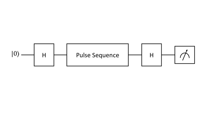
As illustrated by Fig. 1, a general protocol for noise spectroscopy goes as follows: (1) Prepare the system qubit in the $|+\rangle=\frac{1}{\sqrt{2}}(|0\rangle+|1\rangle)$ state using a Hadamard gate. (2) Apply a sequence of $\pi$ pulses, of total time duration $T$. (3) Rotate the qubit back with a Hadamard gate and measure its state in the $\sigma_{z}$ basis. (4) Repeat (1)-(3) many times and estimate the probability, $P_{0}(T)$, to obtain the qubit in the $|0\rangle$ state.

For a stochastic bath, $P_{0}(T)$ yields an exponential decay, $e^{-\chi(T)}$, which only depends on $S(\omega)$ and the pulse sequence [35, 36, 37],

$$P_{0}(T) =\tfrac{1}{2}(1+e^{-\chi(T)}),$$ (5)

$$\chi(T) =\int_{-\infty}^{\infty}\frac{d\omega}{2\pi}S(\omega)|\tilde{f}(\omega)|^{2}=\int_{-\infty}^{\infty}\frac{d\omega}{2\pi}S(\omega)W(\omega),$$

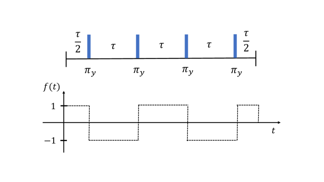
where $f(t)$ is the filter function corresponding to the pulse sequence (see Fig. 1), $\tilde{f}(\omega)$ is the Fourier transform of the filter function, and the window function, $W(\omega)$, is defined as $W(\omega)=|\tilde{f}(\omega)|^{2}$.

[]

[]

[]

Figure 1: (a). A single-qubit noise spectroscopy experiment. The qubit is initialized in the $|+\rangle$ state by a Hadamard gate. Then, the qubit evolves under the application of the pulse sequence. Finally, a measurement is performed in the $\sigma_{z}$ basis after another Hadamard gate. (b). Top: An illustration of the CPMG pulse sequence with $M=4$ instantaneous $\pi$-pulses (blue rectangles) along the $y$ axis. The time interval between each two pulses is $\tau=T/M$. The qubit freely evolves for a time of $\tau/2$ before the first pulse and after the last one. Bottom: The corresponding filter function, $f(t)$, flips the sign every time a $\pi$-pulse is applied. (c) Illustration of the random pulse sequence method. Given a target function, $T(\omega)$, a random pulse generator can produce multiple pulse sequences. The blue spikes represent instantaneous $\pi$-pulses. The expectation value of the resulting window function, $\operatorname{\mathbb{E}}(W(\omega))$, approximates $T(\omega)$. As a result, one can measure the linear functional $\int S(\omega)T(\omega)d\omega$ by averaging the outcome of each individual pulse sequence.

III.1 Dynamical decoupling

Here we review the Carr-Purcell-Meiboom-Gill (CPMG) pulse sequence as the typical DD method used for noise spectroscopy [14, 16, 17, 5, 18, 19, 20, 38]. The CPMG pulse sequence (illustrated by Fig. 1) consists of $M$ rotation $\pi$-pulses applied with time period $\tau$ ($\tau=T/M$). The window function of this sequence equals

$$W(\omega)=\begin{cases}\frac{32}{\omega^{2}}\sin^{4}(\tfrac{\omega\tau}{4})\sin^{2}(\tfrac{\omega M\tau}{2})/\cos^{2}(\tfrac{\omega\tau}{2}),\text{for even $M$}\\ \frac{32}{\omega^{2}}\sin^{4}(\tfrac{\omega\tau}{4})\cos^{2}(\tfrac{\omega M\tau}{2})/\cos^{2}(\tfrac{\omega\tau}{2}),\text{for odd $M$}.\end{cases}$$ (6)

When $M\rightarrow\infty$, we get $W(\omega)\propto T\delta(\pi/2\tau)$ such that

$$\chi(T)\approx\int_{-\infty}^{\infty}\frac{d\omega}{\pi}S(\omega)\frac{4T\delta(\pi/2\tau)}{\pi}\approx\frac{4T}{\pi^{2}}S(\pi/2\tau).$$ (7)

As a result, the application of a CPMG sequence mainly probes the noise at a single frequency of $\pi/2\tau$ (with second order corrections described in [34]). To fully decompose the spectrum then requires sweeping the free evolution time, $\tau$ (or the number of pulses, $M$). However, such probing across the whole frequency range involves numerous measurements, which are not always necessary for extracting the significant features of the noise.

III.2 Random pulse sequence

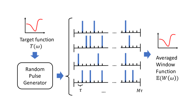
We propose an alternative method for noise spectroscopy based on random pulse sequences. Rather than probing single frequencies like the CPMG method, our approach generates window functions, $W(\omega)$, with desired spectral shapes that probe any linear functional of $S(\omega)$. The general idea is to design a random pulse generator to produce a group of sequences, such that the expectation value of their window function, $\operatorname{\mathbb{E}}(W(\omega))$, can approximate a desired target function, $T(\omega)$ (as illustrated in Fig. 1 and further explained in [34]). As a result, we can directly estimate the linear functional, $I=\int S(\omega)T(\omega)d\omega$. This procedure is analogous to the generation of a stationary sequence [39], adapted for noise spectroscopy.

The random pulse sequences are generated in the following way. The total experiment time, $T$, is divided into $M$ equal segments, such that $T=M\tau$. Rotation $\pi$-pulses are applied only at the end of particular segments determined by a random pulse generator. Specifically, we generate a vector of random variables, $\vec{U}=(U_{1},\ldots,U_{M})\in\{1,-1\}^{M}$, and a corresponding random pulse sequence, such that:

1. $U_{i}$ represents the value of the filter function, $f(t)$, in the time segment $t\in[(i-1)\tau,i\tau]$. A $\pi$-pulse is applied at time $i\tau$ if and only if $U_{i}\neq U_{i+1}$.

2. The expectation value of any random variable is zero, i.e., $\operatorname{\mathbb{E}}(U_{i})=0$.

3. The covariance of two random variables, $U_{i},U_{j}$, should only depend on the distance $\lvert j-i\rvert$, i.e., it has the form $\operatorname{\mathbb{E}}(U_{i}U_{i+j})=R(j)$, where $R(j)$ is determined by the target function, $T(\omega)$, that we wish to generate.

Random variables $U_{i}$ satisfying these properties can be constructed by generating a sequence of independent Gaussian random variables, applying a finite impulse response (FIR) filter with suitably chosen coefficients $(a_{0},a_{1},\ldots,a_{\lambda-1})$, and then applying the sign function. In some cases, time-varying FIR filters may be used for improved computational efficiency [34].

In the following, we show, given a target function $T(\omega)$, which random pulse covariances $R(j)$ should be chosen. The random pulse sequence produces a certain window function, $W_{U}(\omega)$, that probes the noise. The expectation value of the window function over all the possible realizations of $\vec{U}$ yields

$$\small\operatorname{\mathbb{E}}(W_{U}(\omega))=M\tau^{2}\operatorname{sinc}^{2}(\tfrac{\omega\tau}{2})[1+2\sum_{k=1}^{\lambda}R(k)\cos{(k\omega\tau)}(1-\tfrac{k}{M})],$$ (8)

where we define $\operatorname{sinc}x=\tfrac{\sin x}{x}$ and $\lambda$ is the cutoff distance of the correlation between random variables, i.e., $R(k|k>\lambda)=0$.

Note that the cosine functions $\{\cos(k\omega\tau)\}$ form an almost complete basis (the zeroth term excluded) in the region $[-\tfrac{\pi}{\tau},\tfrac{\pi}{\tau}]$. Thus, by matching the time interval between segments and the cutoff frequency of the noise (i.e., setting $\tau=\tfrac{\pi}{\omega_{c}}$), and by adjusting the random pulse generator (i.e., optimizing the filter coefficients $(a_{0},a_{1},\ldots,a_{\lambda-1})$, as explained in [34]) so that

$$R(k)=\tfrac{M}{\pi(M-k)}\int_{-\omega_{c}}^{\omega_{c}}\frac{cT(\omega)\cos(k\omega\tau)}{\operatorname{sinc}^{2}(\tfrac{\omega\tau}{2})}d\omega,$$ (9)

the expectation value of $W(\omega)$ yields

$$\operatorname{\mathbb{E}}(W(\omega))\xrightarrow{\lambda\rightarrow\infty}M\tau^{2}[cT(\omega)+(1-cT_{0})\operatorname{sinc}^{2}(\tfrac{\omega\tau}{2})].$$ (10)

In Eqs. (9) and (10), $c$ is an adjustable parameter that ensures the positivity of $W(\omega)$, and $T_{0}$ is a constant term depending on $T(\omega)$,

$$T_{0}=\tfrac{1}{\omega_{c}}\int_{-\omega_{c}}^{\omega_{c}}\frac{T(\omega)}{\operatorname{sinc}^{2}(\tfrac{\omega\tau}{2})}d\omega.$$ (11)

Note that $R(k)$ is proportional to the $k$-th coefficient of the Fourier series representation of $T(\omega)/\operatorname{sinc}^{2}(\tfrac{\omega\tau}{2})$ (Eq. (9)). As such, Eq. (10) is a good approximation for a finite $\lambda$, if $R(k)$ converges to 0 as $k\rightarrow\infty$. By plugging Eq. (10) into Eq. (5), the expectation value of the decay exponent yields

$$\small\operatorname{\mathbb{E}}(\chi)=\frac{M\tau^{2}}{2\pi}\int_{-\omega_{c}}^{\omega_{c}}[cT(\omega)S(\omega)d\omega+(1-cT_{0})\operatorname{sinc}^{2}(\tfrac{\omega\tau}{2})S(\omega)d\omega].$$ (12)

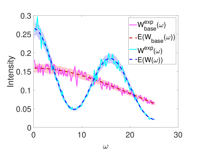
From Eq. (12), we can extract the desired functional, $I=\int S(\omega)T(\omega)d\omega$, by subtracting the term $\int S(\omega)\operatorname{sinc}^{2}(\tfrac{\omega\tau}{2})d\omega$ from $\operatorname{\mathbb{E}}(\chi)$. This term can be estimated by applying an additional series of “base” random pulse sequences, for which $\vec{U}$ contains independent random variables (that is, $R(k)=0$ for all $k>0$). The expectation value of the “base” sequence’s window function is $\operatorname{\mathbb{E}}(W_{\text{base}}(\omega))=\tfrac{M\tau^{2}}{2\pi}\operatorname{sinc}^{2}(\tfrac{\omega\tau}{2})$, and the corresponding decay exponent is $\operatorname{\mathbb{E}}(\chi_{\text{base}})=\tfrac{1}{2\pi}\int S(\omega)\operatorname{\mathbb{E}}(W_{\text{base}}(\omega))$. Figure 2 illustrates the window functions generated by the random pulse protocol for a target function of $T_{1}(\omega)=\operatorname{sinc}^{2}{(\tfrac{\omega\tau}{2})}\cos{(3\omega\tau)}$. The value of $\operatorname{\mathbb{E}}(W_{base})$ (dashed magenta line in Fig. 2) is subtracted from $\operatorname{\mathbb{E}}(W(\omega))$ (dashed cyan line in Fig. 2), to obtain $T(\omega)$ (dashed cyan line in Fig. 2).

[]

[]

Figure 2: Illustration of the generation of the target function ${T}(\omega)=\operatorname{sinc}^{2}{(\tfrac{\omega\tau}{2})}\cos{(3\omega\tau)}$ by two groups of random pulses. In both plots, the dashed lines represent exact expectation values. The solid lines represent simulated results of an experimental realization considering 200 random pulse sequences with 50 segments, each repeated 200 times. The shaded area represents the uncertainties of these results. (a) The dashed blue line (dashed red line) stands for the expectation value of the window function, $\operatorname{\mathbb{E}}(W(\omega))$ (of the base window function, $\operatorname{\mathbb{E}}(W_{\text{base}}(\omega)$)), generated by ${T}(\omega)$, and the solid cyan line (solid magenta line) is the corresponding simulation of the experimental result, $W^{\text{exp}}(\omega)$ ($W_{\text{base}}^{\text{exp}}(\omega)$). (b) The dashed blue line represents ${T}(\omega)$. The solid cyan line stands for the extracted window function of the two averaged window functions in (a), calculated by ${W^{*}(\omega)}=[W^{\text{exp}}(\omega)-(1-cT_{0})W_{\text{base}}^{\text{exp}}(\omega)]/c$.

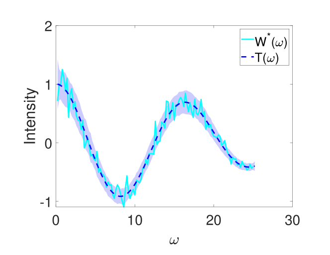
The experimental estimation of the desired functional, $I^{\text{exp}}$, requires measuring the decay exponent $\chi^{\text{exp}}$, by generating $N_{1}$ different random pulse sequences with each repeated $N_{2}$ times, as well as measuring the base decay exponent, $\chi_{\text{base}}^{\text{exp}}$, by generating $N_{\text{base},1}$ different random pulse sequences with each repeated $N_{\text{base},2}$ times. For the specific target function $T(\omega)$ in Fig. 2, the application of random pulse sequences with $(M,N_{1},N_{2})=(M,N_{\text{base},1},N_{\text{base},2})=(200,200,50)$ (solid lines in Fig. 2) provides a close estimation of the expectation values (dashed lines in Fig. 2).

IV Accuracy of the method

The accuracy of the experimental estimation of the desired functional, $I^{\text{exp}}$, depends on the accuracies of the experimentally measured decay exponents, which are also yielded by the method to generate random pulses. For a specific type of random pulse generator, the accuracy is given by (see [34])

$$|\chi^{\text{exp}} -\operatorname{\mathbb{E}}(\chi)|$$ (13)

$$= O\bigg{(}\sqrt{\frac{2}{\pi M\tau}}\frac{||S(\omega)\operatorname{\mathbb{E}}(W(\omega))-\langle S(\omega)\operatorname{\mathbb{E}}(W(\omega))\rangle||_{L2}}{\sqrt{N_{1}}}$$

$$+\frac{||S(\omega)\operatorname{\mathbb{E}}(W(\omega))||_{L1}}{\sqrt{N_{1}N_{2}}}\bigg{)},$$

and the same expression for $|\chi^{\text{exp}}_{\text{base}}-\operatorname{\mathbb{E}}(\chi_{\text{base}})|$ with $\operatorname{\mathbb{E}}(W_{\text{base}}(\omega))=M\tau^{2}\operatorname{sinc}^{2}(\tfrac{\omega\tau}{2})$. In Eq. (13), $\langle.\rangle$ denotes averaging in the frequency regime $[-\pi/\tau,\pi/\tau]$.

The first term in Eq. (13) related to the $L_{2}$ norm can be viewed as a measure of the smoothness of $S(\omega)\operatorname{\mathbb{E}}(W(\omega))$. For example, in the extreme case of constant $S(\omega)\operatorname{\mathbb{E}}(W(\omega))$, the $L_{2}$ norm vanishes. However, when $S(\omega)\operatorname{\mathbb{E}}(W(\omega))$ consists of isolated peaks, the first term will dominate the value of the deviation. In the general case, the best strategy for minimizing the deviation between the measured and ideal decay exponent is to make $N_{1}$ large while keeping $N_{2}$ as small as possible [34].

V Compressed sensing

[]

[]

Figure 3: (a) A reconstruction of an ideal sparse spectrum using the CS method. The solid blue line represents a 2-sparse spectrum with $N=250$ grid points. The red circles represent the decomposed spectrum using CS based on $m=12$ different Fourier basis functions. For each Fourier basis function, we generate random pulse sequences with $(M,N_{1},N_{2})=(250,1000,50)$. (b) The accuracy of CS ($(M,N_{1},N_{2})=(250,1000,50)$) in reconstructing ideal spectra as a function of the number of Fourier basis functions. Different curves represent different sparsities considering 200 randomly generated spectra with $N=250$. Each simulation is repeated for 100 times and the shaded areas represent the 95% confidence regime. Inset: The scaling of the critical number of Fourier basis functions, $m_{c}$, as a function of the sparsity of the spectrum.

Figure 4: A reconstruction of the noise spectrum of an ensemble of nuclear spins interacting with an InAs/GaAs quantum dot (under an external magnetic field of B = 2 T at the Voigt geometry) using pulse sequences of compressed sensing. The blue solid line represents the theoretically simulated noise spectrum. The red dots represent the simulated reconstructed spectrum considering random pulse sequences with $(M,N_{1},N_{2})=(200,2000,50)$ and $m=40$ different Fourier basis functions. For the CS method, we estimate the spectrum using the LASSO, with $N=667$ grid points and 10-fold cross validation, which successfully identifies the central frequencies of the major peaks.

Figure 5: Numerical simulations of the accuracy of reconstructing the central frequencies of the InAs/GaAs noise spectrum as a function of the number of sets of experiments, $N_{\text{set}}$. The reconstruction accuracy, $|\hat{\omega}^{*}-\hat{\omega}^{\text{th}}|_{\infty}$, quantifies the deviation between the reconstructed frequencies and the theoretical ones for the three largest peaks. The solid blue line and the dashed red line represent the accuracy of CS with $N=167$ and $N=667$ grid points, respectively. The CS simulations are repeated for 30 times and the shaded areas represents the 95% confidence regimes. The dotted green line represents the reconstruction accuracy of the noise spectrum using the CPMG sequences. Achieving a certain accuracy by utilizing the CPMG sequences requires an order of magnitude more sets of experiments than by utilizing CS.

A promising application of the random pulse method is the compressed sensing (CS) [25, 26] of sparse noise spectra. A noise spectrum, approximated as a function on a discrete subset of $N$ points in the frequency domain (call this subset $G_{N}$), is called $s$-sparse if it contains at most $s$ non-zero elements. As we show below, our method implements $O(s\log N)$ sets of random pulses to fully decompose the spectrum, ideally providing an exponential speedup compared to $O(N)$ sets of experiments required by the CPMG protocol.

The main idea of the CS method is to implement random pulse sequences that generate a random set of Fourier basis functions to probe the spectrum. According to equations (8) and (10), the target function of random pulse sequences can be set to $T_{k}(\omega)=\cos(k\omega\tau)\operatorname{sinc}^{2}(\tfrac{\omega\tau}{2})$ by setting $R(j)=\tfrac{M}{2(M-k)}\delta(j-k)$, such that

$$\operatorname{\mathbb{E}}(\chi_{k}-\chi_{\text{base}})=M\tau^{2}\int_{-\omega_{c}}^{\omega_{c}}S(\omega)\operatorname{sinc}^{2}(\tfrac{\omega\tau}{2})\cos(k\omega\tau)d\omega,$$ (14)

where $\chi_{k}$ is the decay exponent for random pulses with $T_{k}(\omega)$. Note that the term $S(\omega)\operatorname{sinc}^{2}(\tfrac{\omega\tau}{2})$ has the same sparsity as $S(\omega)$, since $\operatorname{sinc}^{2}(\tfrac{\omega\tau}{2})$ varies mildly between $\tfrac{4}{\pi^{2}}$ and $1$ when $\omega$ is in the interval $[-\tfrac{\pi}{\tau},\tfrac{\pi}{\tau}]$.

According to the CS theory [25, 26], by generating $m$ random Fourier functions with frequencies $k_{1},\ldots,k_{m}$, the discrete spectrum $S^{*}:\>G_{N}\rightarrow\mathbb{R}$ (where $G_{N}$ is the set of grid points) can be recovered by solving a convex optimization problem,

$$\min_{{S^{*}:\>G_{N}\rightarrow\mathbb{R}}}||S^{*}(\omega)\operatorname{sinc}^{2}(\omega\tau/2)||_{L_{1}},\text{ subject to}$$ (15)

$${\sum_{j=1}^{m}\biggl{\lvert}}\chi^{\text{exp}}_{k_{j}}-\chi^{\text{exp}}_{\text{base}}$$

$$-\frac{2\omega_{c}M\tau^{2}}{N}||S^{*}(\omega)\operatorname{sinc}^{2}(\omega\tau/2)\cos(k_{j}\omega\tau)||_{L_{1}}{\biggr{\rvert}^{2}\leq\epsilon}.$$

Here, $\epsilon$ is chosen by the experimenter to allow for noise in the measurements of $\chi^{\text{exp}}_{k_{j}}$ and $\chi^{\text{exp}}_{\text{base}}$. The solution $S^{*}(\omega)$ to Eq. (15) is accurate if the number of generated Fourier functions satisfies $m\geq{\Omega}(s\log N)$ [26].

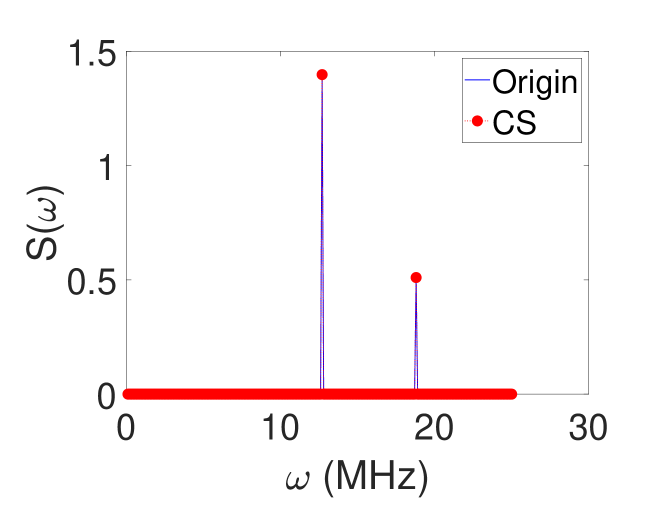
Fig. 3 presents a numerical simulation of the CS method on an ideal sparse spectrum. The solid blue line represents a 2-sparse spectrum with $N=250$ grid points. The red circles represent the reconstructed spectrum, $S^{*}(\omega)$, obtained from CS with $m=12$ different Fourier basis functions. By accurately identifying the non-zero elements of the original spectrum (blue line), the CS method (red circles) succeeeds in reconstructing it.

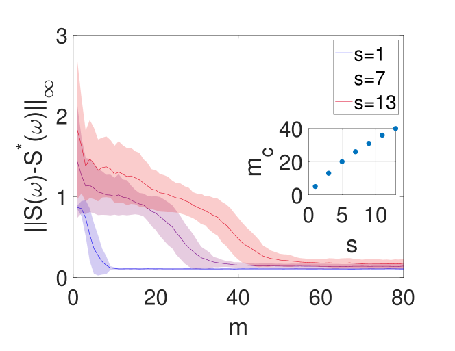
We further examine the accuracy of CS in reconstructing ideal spectra under different sparsities, $s$, as a function of the number of Fourier basis functions, $m$ (Fig. 3). For each sparsity (different curves in Fig. 3), we randomly generate 200 sparse spectra with $N=250$ grid points to obtain the averaged accuracy (see [34]). The accuracy is defined as the $L_{\infty}$ norm of the difference between the discretized true spectrum, $S(\omega)$, and the reconstructed spectrum, $S^{*}(\omega)$. For each sparsity, the accuracy undergoes a clear phase transition at a certain value of $m$. We define $m_{c}$ as the critical number of Fourier basis functions for which the accuracy reaches 0.5 (e.g., for $s=13$, $m_{c}=40$). It can be seen that $m_{c}$ is a linear function of $s$ (inset of Fig.3), which is consistent with the theoretically-predicted proportionality between $m$ and $s\log N$.

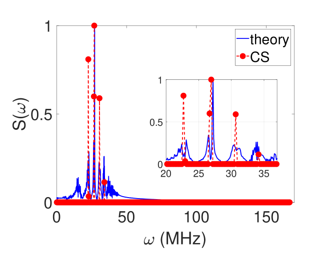
Next, to quantify the performance of the CS method for realistic physical systems, we explore the ability of the method to extract the spectral density of noise that interacts with InAs/GaAs quantum dots. This noise represents the decoherence of the quantum dots due to their hyperfine interaction with an ensemble of nuclear spins broadened by strain [40, 38]. The solid blue line in Fig. 4 shows the theoretical spectral density of such a noise source calculated from the Fourier transform of the autocorrelators of the fluctuating nuclear spins, while considering quantum dots of pure indium and arsenic at a temperature of 4 K and under a magnetic field of B = 2 T applied perpendicular to the growth direction of the dots (Voigt geometry) [40]. This spectrum consists of several narrow peaks at spectral frequencies that correspond to different Larmor frequencies of the nuclei.

The red dots in Fig. 4 represent the discrete spectrum obtained by simulating the performance of CS with $m=40$ different Fourier basis functions. While the theoretical spectrum is not ideally sparse, we adopt suitable data analysis techniques (least absolute shrinkage and selection (LASSO) [41], along with cross-validation (CV) [34]) to successfully identify the centers of the major peaks.

We quantify the accuracy of extracting the InAs/GaAs noise spectrum by comparing the central frequencies of the largest three peaks obtained from CS to their theoretical values. The theoretical central frequencies, $\hat{\omega}^{\text{th}}=(\omega_{1},\omega_{2},\omega_{3})$, are calculated by a Gaussian fitting to the theoretical spectrum. The experimental results, $\hat{\omega}^{*}=(\omega_{1}^{*},\omega_{2}^{*},\omega_{3}^{*})$, are the weighted mean values of the frequencies from the neighboring non-zero discrete $S^{*}(\omega)$ obtained from CS. The reconstruction accuracy is defined as the $\ell_{\infty}$ norm of the difference between these two vectors, i.e. $|\hat{\omega}^{*}-\hat{\omega}^{\text{th}}|_{\infty}$.

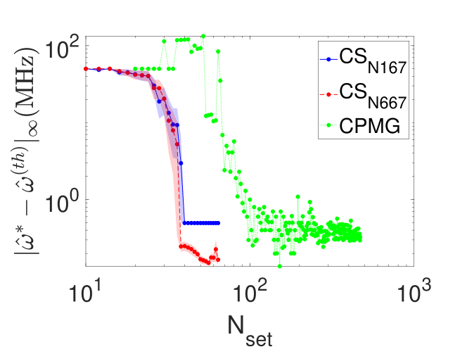
The solid blue line and the dashed red line in Fig. 5 represent the simulated reconstruction accuracies of CS with $N=167$ and $N=667$ grid points, respectively. In these simulations, we assume no experimental errors and only focus on the effect of the number of different sets of experiments, $N_{\text{set}}$. For CS, $N_{\text{set}}=m+1$ for $m$ Fourier basis functions and one additional experiment with the base random pulse sequence. For both choices of $N$, we observe a sharp change (phase transition) in the accuracy of reconstructing the spectrum at $N_{\text{set}}\approx 40$. The reconstruction accuracies then converge to constant values inversely proportional to $N$ (e.g., the dashed red line for $N=667$ has a lower baseline than the solid blue line for $N=167$). As a result, increasing the number of grid points $N$ in post-processing could boost the spectral resolution of CS without adding any resources.

To further demonstrate the resource efficiency of the CS method, we compare the accuracies of CS in resolving the InAs/GaAs noise spectrum to the ones obtained by using the conventional CPMG method (dotted green line in Fig. 5). For CPMG, the number of sets of experiments required for noise spectroscopy is given by $N_{\text{set}}={2\omega_{c}T}/{\pi}$, i.e., the number of different sequences that probe the noise spectrum over the frequency range $[0,\omega_{c}]$ given the total experiment time, $T$ [14, 16, 17, 5, 18, 19, 20, 38].

For $N_{\text{set}}<100$, the CPMG sequences cannot resolve adjacent spectral peaks of the InAs/GaAs noise spectrum (i.e., $|\hat{\omega}^{*}-\hat{\omega}^{\text{th}}|_{\infty}>1$), because the sampling frequency interval associated with the sequences is wider than the spectral distance between nearby peaks in the spectrum. Meanwhile, for $N_{\text{set}}>100$, the CPMG protocol can resolve the desired spectrum, with accuracy inversely proportional to $N_{\text{set}}$. However, to achieve a certain level of accuracy, the CPMG sequences require at least an order of magnitude more resources than the CS method. For example, as we illustrate for the InAs/GaAs noise spectrum, $|\hat{\omega}^{*}-\hat{\omega}^{\text{th}}|_{\infty}\approx 0.2$ for CS dashed red line) with $N=667$ grid points and $N_{set}\approx 40$; but this accuracy is hardly reached by CPMG (dotted green line) up to $N_{set}\approx 500$.

VI Outlook

To conclude, we develop a new method for qubit noise spectroscopy based on the realization of random pulse sequences. This method allows us to measure arbitrary linear functionals of the noise spectrum, and reconstruct sparse spectra by utilizing compressed sensing (CS). Furthermore, the proposed method can be used to reconstruct noise spectra of realistic physical systems, such as optically-active quantum dots, with an order of magnitude less resources than conventional dynamical decoupling techniques.

For future research, our method can be generalized to incorporate pulses with durations other than $\pi$, and toward the characterization of multi-qubit systems [12]. In addition, while we have only considered the reconstruction of the noise spectrum on a finite set of sample points, similar ideas can be applied to reconstruction over continuous domains [42, 43, 44].

Finally, the accuracy of CS utilizing random pulse sequences strongly depends on the spectral properties of the probed noise source. Beyond the experimental realization of CS on the specific platform of InAs/GaAs quantum dots, it would be beneficial to study the performance of random pulse sequences on realistic noise sources with various spectral features, e.g., levels of sparsity.

VII Acknowledgements

It is a pleasure to thank Gregory Quiroz, Kevin Schultz, and others at the Johns Hopkins University Applied Physics Laboratory, for helpful discussions. This work was partially supported by an AFOSR MURI on Scalable Certification of Quantum Computing Devices and Networks, a DOE ASCR ARQC award on Fundamental Algorithmic Research for Quantum Computing (FAR-QC), and the NSF QLCI for Robust Quantum Simulation (RQS). A.S. acknowledges support from a Chicago Prize Postdoctoral Fellowship in Theoretical Quantum Science.

References

- [1] F. Yan, J. Bylander, S. Gustavsson, F. Yoshihara, K. Harrabi, D. G. Cory, T. P. Orlando, Y. Nakamura, J.-S. Tsai, and W. D. Oliver, “Spectroscopy of low-frequency noise and its temperature dependence in a superconducting qubit,” Phys. Rev. B, vol. 85, p. 174521, May 2012.
- [2] O. E. Dial, M. D. Shulman, S. P. Harvey, H. Bluhm, V. Umansky, and A. Yacoby, “Charge noise spectroscopy using coherent exchange oscillations in a singlet-triplet qubit,” Phys. Rev. Lett., vol. 110, p. 146804, Apr 2013.
- [3] J. T. Muhonen, J. P. Dehollain, A. Laucht, F. E. Hudson, R. Kalra, T. Sekiguchi, K. M. Itoh, D. N. Jamieson, J. C. McCallum, A. S. Dzurak, et al., “Storing quantum information for 30 seconds in a nanoelectronic device,” Nature nanotechnology, vol. 9, no. 12, pp. 986–991, 2014.
- [4] F. Reinhard, F. Shi, N. Zhao, F. Rempp, B. Naydenov, J. Meijer, L. T. Hall, L. Hollenberg, J. Du, R.-B. Liu, and J. Wrachtrup, “Tuning a spin bath through the quantum-classical transition,” Phys. Rev. Lett., vol. 108, p. 200402, May 2012.
- [5] N. Bar-Gill, L. M. Pham, C. Belthangady, D. Le Sage, P. Cappellaro, J. Maze, M. D. Lukin, A. Yacoby, and R. Walsworth, “Suppression of spin-bath dynamics for improved coherence of multi-spin-qubit systems,” Nature communications, vol. 3, no. 1, pp. 1–6, 2012.
- [6] Y. Romach, C. Müller, T. Unden, L. J. Rogers, T. Isoda, K. M. Itoh, M. Markham, A. Stacey, J. Meijer, S. Pezzagna, B. Naydenov, L. P. McGuinness, N. Bar-Gill, and F. Jelezko, “Spectroscopy of surface-induced noise using shallow spins in diamond,” Phys. Rev. Lett., vol. 114, p. 017601, Jan 2015.
- [7] C. L. Degen, F. Reinhard, and P. Cappellaro, “Quantum sensing,” Rev. Mod. Phys., vol. 89, p. 035002, Jul 2017.
- [8] T. Yuge, S. Sasaki, and Y. Hirayama, “Measurement of the noise spectrum using a multiple-pulse sequence,” Physical review letters, vol. 107, no. 17, p. 170504, 2011.
- [9] G. A. Álvarez and D. Suter, “Measuring the spectrum of colored noise by dynamical decoupling,” Phys. Rev. Lett., vol. 107, p. 230501, Nov 2011.
- [10] K. C. Young and K. B. Whaley, “Qubits as spectrometers of dephasing noise,” Phys. Rev. A, vol. 86, p. 012314, Jul 2012.
- [11] L. M. Norris, G. A. Paz-Silva, and L. Viola, “Qubit noise spectroscopy for non-gaussian dephasing environments,” Phys. Rev. Lett., vol. 116, p. 150503, Apr 2016.
- [12] G. A. Paz-Silva, L. M. Norris, and L. Viola, “Multiqubit spectroscopy of gaussian quantum noise,” Phys. Rev. A, vol. 95, p. 022121, Feb 2017.
- [13] C. Ferrie, C. Granade, G. Paz-Silva, and H. M. Wiseman, “Bayesian quantum noise spectroscopy,” New Journal of Physics, vol. 20, p. 123005, dec 2018.
- [14] U. Haeberlen, Advances in magnetic resonance, vol. 1. Academic Press, 1976.
- [15] L. M. Vandersypen and I. L. Chuang, “Nmr techniques for quantum control and computation,” Reviews of modern physics, vol. 76, no. 4, p. 1037, 2005.
- [16] J. Bylander, S. Gustavsson, F. Yan, F. Yoshihara, K. Harrabi, G. Fitch, D. G. Cory, Y. Nakamura, J.-S. Tsai, and W. D. Oliver, “Noise spectroscopy through dynamical decoupling with a superconducting flux qubit,” Nature Physics, vol. 7, no. 7, pp. 565–570, 2011.
- [17] Y.-X. Wang and A. A. Clerk, “Intrinsic and induced quantum quenches for enhancing qubit-based quantum noise spectroscopy,” Nature communications, vol. 12, no. 1, pp. 1–14, 2021.
- [18] F. K. Malinowski, F. Martins, P. D. Nissen, E. Barnes, Ł. Cywiński, M. S. Rudner, S. Fallahi, G. C. Gardner, M. J. Manfra, C. M. Marcus, et al., “Notch filtering the nuclear environment of a spin qubit,” Nature nanotechnology, vol. 12, no. 1, pp. 16–20, 2017.
- [19] K. Chan, W. Huang, C. Yang, J. Hwang, B. Hensen, T. Tanttu, F. Hudson, K. M. Itoh, A. Laucht, A. Morello, et al., “Assessment of a silicon quantum dot spin qubit environment via noise spectroscopy,” Physical Review Applied, vol. 10, no. 4, p. 044017, 2018.
- [20] T. Yuge, S. Sasaki, and Y. Hirayama, “Measurement of the noise spectrum using a multiple-pulse sequence,” Physical review letters, vol. 107, no. 17, p. 170504, 2011.
- [21] F. Serinaldi and F. Lombardo, “Betabit: A fast generator of autocorrelated binary processes for geophysical research,” Europhysics Letters, vol. 118, no. 3, p. 30007, 2017.
- [22] F. Serinaldi and F. Lombardo, “General simulation algorithm for autocorrelated binary processes,” Physical Review E, vol. 95, no. 2, p. 023312, 2017.
- [23] K. Schultz, G. Quiroz, P. Titum, and B. Clader, “Schwarma: A model-based approach for time-correlated noise in quantum circuits,” Physical Review Research, vol. 3, no. 3, p. 033229, 2021.
- [24] A. Murphy, J. Epstein, G. Quiroz, K. Schultz, L. Tewala, K. McElroy, C. Trout, B. Tien-Street, J. A. Hoffmann, B. Clader, et al., “Universal-dephasing-noise injection via schrödinger-wave autoregressive moving-average models,” Physical Review Research, vol. 4, no. 1, p. 013081, 2022.
- [25] E. J. Candès and M. B. Wakin, “An introduction to compressive sampling,” IEEE Signal Processing Magazine, vol. 25, no. 2, pp. 21–30, 2008.
- [26] E. J. Candes and Y. Plan, “A probabilistic and ripless theory of compressed sensing,” IEEE Transactions on Information Theory, vol. 57, no. 11, pp. 7235–7254, 2011.
- [27] K. Seetharam, D. Biswas, C. Noel, A. Risinger, D. Zhu, O. Katz, S. Chattopadhyay, M. Cetina, C. Monroe, E. Demler, and D. Sels, “Digital quantum simulation of NMR experiments,” tech. rep., Arxiv preprint 2109.13298, 2021.
- [28] M. Bostock and D. Nietlispach, “Compressed sensing: Reconstruction of non-uniformly sampled multidimensional nmr data,” Concepts in Magnetic Resonance Part A, vol. 46, no. 2, p. e21438, 2017.
- [29] H. Breuer and F. Petruccione, The Theory Of Open Quantum Systems. USA: Oxford University Press, 2002.
- [30] U. Weiss, Quantum Dissipative Systems,. Singapore: World Scientific, 1993.
- [31] L. Viola, E. Knill, and S. Lloyd, “Dynamical decoupling of open quantum systems,” Physical Review Letters, vol. 82, no. 12, p. 2417, 1999.
- [32] K. Khodjasteh, T. Erdélyi, and L. Viola, “Limits on preserving quantum coherence using multipulse control,” Physical Review A, vol. 83, no. 2, p. 020305, 2011.
- [33] A. J. Leggett, S. Chakravarty, A. T. Dorsey, M. P. Fisher, A. Garg, and W. Zwerger, “Dynamics of the dissipative two-state system,” Reviews of Modern Physics, vol. 59, no. 1, p. 1, 1987.
- [34] K. Huang, D. Farfurnik, A. Seif, M. Hafezi, and Y.-K. Liu, “Random pulse sequences for qubit noise spectroscopy (supplementary material),” 2023. In preparation.
- [35] G. A. Paz-Silva and L. Viola, “General transfer-function approach to noise filtering in open-loop quantum control,” Phys. Rev. Lett., vol. 113, p. 250501, Dec 2014.
- [36] G. A. Paz-Silva, L. M. Norris, and L. Viola, “Multiqubit spectroscopy of gaussian quantum noise,” Phys. Rev. A, vol. 95, p. 022121, Feb 2017.
- [37] L. Cywiński, R. M. Lutchyn, C. P. Nave, and S. Das Sarma, “How to enhance dephasing time in superconducting qubits,” Phys. Rev. B, vol. 77, p. 174509, May 2008.
- [38] D. Farfurnik, H. Singh, Z. Luo, A. S. Bracker, S. G. Carter, R. M. Pettit, and E. Waks, “All-optical noise spectroscopy of a solid-state spin,” arXiv preprint arXiv:2109.03405, 2021.
- [39] M. Rosenblatt, Stationary sequences and random fields. Springer Science & Business Media, 2012.
- [40] R. Stockill, C. Le Gall, C. Matthiesen, L. Huthmacher, E. Clarke, M. Hugues, and M. Atatüre, “Quantum dot spin coherence governed by a strained nuclear environment,” Nature communications, vol. 7, no. 1, pp. 1–7, 2016.
- [41] T. Hastie, R. Tibshirani, J. H. Friedman, and J. H. Friedman, The elements of statistical learning: data mining, inference, and prediction, vol. 2. Springer, 2009.
- [42] E. J. Candès and C. Fernandez-Granda, “Towards a mathematical theory of super-resolution,” Communications on Pure and Applied Mathematics, vol. 67, no. 6, pp. 906–956, 2014.
- [43] G. Tang, B. N. Bhaskar, P. Shah, and B. Recht, “Compressed sensing off the grid,” IEEE Transactions on Information Theory, vol. 59, no. 11, pp. 7465–7490, 2013.
- [44] Y. Chi and M. F. Da Costa, “Harnessing sparsity over the continuum: Atomic norm minimization for superresolution,” IEEE Signal Processing Magazine, vol. 37, no. 2, pp. 39–57, 2020.