Stochastic Clustered Federated Learning

Abstract

Federated learning is a distributed learning framework that takes full advantage of private data samples kept on edge devices. In real-world federated learning systems, these data samples are often decentralized and Non-Independently Identically Distributed (Non-IID), causing divergence and performance degradation in the federated learning process. As a new solution, clustered federated learning groups federated clients with similar data distributions to impair the Non-IID effects and train a better model for every cluster. This paper proposes StoCFL, a novel clustered federated learning approach for generic Non-IID issues. In detail, StoCFL implements a flexible CFL framework that supports an arbitrary proportion of client participation and newly joined clients for a varying FL system, while maintaining a great improvement in model performance. The intensive experiments are conducted by using four basic Non-IID settings and a real-world dataset. The results show that StoCFL could obtain promising cluster results even when the number of clusters is unknown. Based on the client clustering results, models trained with StoCFL outperform baseline approaches in a variety of contexts.

1 Introduction

Federated learning (FL) (McMahan et al., 2017; Yang et al., 2019) allows smart devices or institutions to collaboratively conduct machine learning tasks without violating privacy regulations. In this way, data collected on mobile phones and personal computers could be fully utilized by the framework. Furthermore, these data samples usually contain habits, preferences, and even geographic information. Hence, the distribution of data samples among devices in this decentralized system can be quite heterogeneous. Previous research (Zhao et al., 2018; McMahan et al., 2017; Li et al., 2020a, 2022; Zeng et al., 2022a) has revealed that the heterogeneous distribution of data between FL devices can cause divergence or slow convergence in the FL training process, which is referred to as Non-Independently Identically Distributed (Non-IID) issues.

Clustered federated learning (CFL) (Sattler et al., 2020a, b; Ghosh et al., 2020; Briggs et al., 2020; Duan et al., 2021) is an approach to address the Non-IID issues by clustering clients with similar data distributions and learning a personalized model for each cluster. In this case, the Non-IID issues are negligible within the clusters that can be solved easily. Typically, the CFL is built on an assumption, i.e.,

Assumption 1 (Clustered Federated Learning (Sattler et al., 2020a)).

There exists a partitioning $\mathcal{C}=\{c_{1},\dots,c_{K}\},\bigcup_{k=1}^{K}c_{k}=\{1,\dots,N\}$ ($N\geq K\geq 2$) of the client population, such that every subset of clients $c_{k}\in\mathcal{C}$ satisfies the distribution learning assumption (i.e., the data distribution among these clients is similar).

It is assumed that clients in the same group have a similar data distribution. Hence, FedAvg (McMahan et al., 2017) can thus fit data samples in the same cluster very well as long as the clustering goal is fulfilled. Meanwhile, the convergence study of such a CFL pattern is given in  (Ma et al., 2022). However, a number of actual limitations are not considered in existing CFL algorithms for real-world applications. For example, some CFL algorithms (Sattler et al., 2020a; Stallmann and Wilbik, 2022; Duan et al., 2021) require all clients to participate in the FL process. However, federated devices are not always online in real-world applications, especially in cross-device settings. Other studies (Ghosh et al., 2020; Wang et al., 2022; Mansour et al., 2020) necessitate information about the number of clusters, which is often difficult to get in real-world systems due to privacy constraints. As a result, incorrectly estimating the number of clusters may hamper the FL models’ performance. Overall, the application opportunities for CFL approaches are limited due to these severe constraints. Therefore, it is necessary to study a flexible and practical clustered federated learning framework for unknown and Non-IID data in FL scenarios.

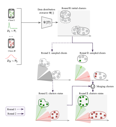
(a) Stochastic Client Clustering

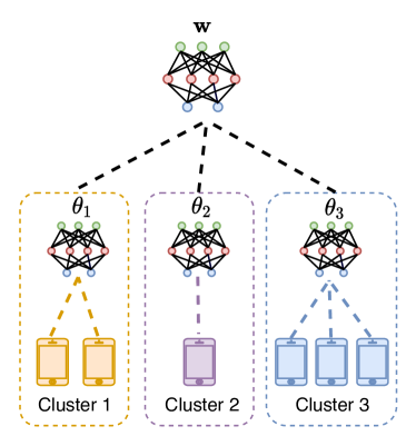
(b) Bi-level Clustered Federated Learning

Figure 1: StoCFL consists of two vital components: stochastic client clustering and bi-level clustered federated learning. In Figure 1(a), the distribution extractor $\Psi(\cdot)$ draws local data distribution representation. Then, the server randomly samples a subset of clients for each round and merges clients into clusters based on cosine similarity. Compared with conventional CFL algorithms (in dashed boxes), Figure 1(b) illustrates an example with 3 clusters that StoCFL enables cluster models to improve each other via a global model $\bm{w}$.

In this research, we introduce StoCFL, a novel CFL algorithm that does not require the number of clusters to be known in advance. Besides, StoCFL allows an arbitrary number of clients to participate in each FL round. In detail, StoCFL creates a representation of local data distributions and evaluates the distribution similarity of any two clients via cosine similarity. Based on this, we implement stochastic federated client clustering, which solves the client clustering problem in that only a subset of clients participates in each round. Furthermore, we propose a bi-level CFL algorithm that enables a knowledge-sharing scheme to further enhance the model performance. Our experimental results show that stochastic federated client clustering can produce promising cluster results in various Non-IID scenarios, while the cluster models trained with StoCFL outperform conventional CFL techniques. In summary, our contributions are as follows.

• We present StoCFL, a novel CFL approach that includes stochastic client clustering and bi-level CFL. StoCFL is flexible with the proportion of client participation and supports newly joined clients in a varying FL system.

• For stochastic client clustering, we suggest a method for drawing a representation of decentralized and inaccessible datasets from federated clients. Then, we estimate the similarity of any two clients via cosine similarity on the representation. Further client clustering trials on four basic Non-IID setups illustrate the client clustering procedure efficacy.

• We assess the performance of StoCFL models on four Non-IID settings and the real-world dataset FEMNIST, including both cross-device (4,800 clients) and cross-silo settings (20 clients). The results of the experiments show that StoCFL outperforms baseline CFL approaches while maintaining a higher generalization performance and system flexibility.

2 Related Work

Non-IID Data Issue. FedAvg (McMahan et al., 2017) could solve the decentralized data optimization problem when these decentralized data are IID. However, in real-world federated learning, the data distributions are usually Non-IID. In this case, FedAvg would take more rounds to iterate the FL model under the Non-IID data setting. The mathematical analysis of this issue in FL is given by work (Zhao et al., 2018), which reveals that the local updates from Non-IID clients are divergent. It consequently damages the convergence performance of FedAvg. Following this study (Hsieh et al., 2020), we review four Non-IID scenarios that widely exist in real-world applications. They are summarized below.

• Feature distribution skew: The marginal distribution of label $\mathcal{P}(x)$ varies across clients. In a handwriting recognition task, the same words written by different users may differ in stroke width, slant, etc.

• Label distribution skew: The marginal distribution of label $\mathcal{P}(y)$ may vary across clients. For instance, clients’ data samples are tied to geo-regions - kangaroos are only in Australia or zoos; for an online shopping website, customers only buy certain items with specific preferences.

• Feature concept skew: The condition distributions $\mathcal{P}(x|y)$ varies across clients, and $\mathcal{P}(y)$ is the same. In other words, the same label $y$ can indicate different features $x$ in different FL clients. For instance, the images of items could vary widely at different times and with different illumination. Hence, the data samples with the same label could look very different.

• Label concept skew: The condition distributions $\mathcal{P}(y|x)$ varies across clients and $\mathcal{P}(x)$ is the same. Similar feature representations from different clients could have different labels because of personal preferences, and the same sentences may reflect different sentiments in language text.

Furthermore, data samples in clients may be a hybrid distribution of the foregoing scenarios in real-world situations, posing a new and formidable challenge to FL techniques. To tackle these Non-IID data issues, conventional federated learning algorithms  (Li et al., 2020b; Acar et al., 2021; Oh et al., 2022; Zeng et al., 2022b) try to learn a single global model that generalizes to all distributions. Another line of research (Li et al., 2021a; Marfoq et al., 2021; T Dinh et al., 2020) focuses on learning personalized models for each client.

Clustered Federated Learning. Clustered federated learning (CFL) is a strategy for dealing with Non-IID difficulties in federated learning. We classify this technique as a compromise between traditional federated learning and personalized federated learning. The first CFL framework is proposed in (Sattler et al., 2020a, b). Other studies follow the CFL-based framework (Ghosh et al., 2020; Briggs et al., 2020; Duan et al., 2021). The core assumption of CFL is described in Assumption 1. Clients with comparable data-generating distributions should be clustered, according to this assumption. The conventional machine learning assumptions would be satisfied by the decentralized datasets in the same cluster.

CFL approaches typically include a federated client clustering algorithm and a cluster model updating algorithm. Federated client clustering is a technique for identifying and grouping clients who have similar data distributions. For example, Works (Stallmann and Wilbik, 2022; Duan et al., 2021; Pedrycz, 2021; Wang et al., 2022; Xie et al., 2020) clusters clients using K-means clustering based on client parameters. CFL (Sattler et al., 2020a, b) separates clients into two partitions, which are congruent. FL+HC (Briggs et al., 2020) uses local updates to produce hierarchical clustering. IFCA (Ghosh et al., 2020)/HypCluster (Mansour et al., 2020) implicitly clusters clients by broadcasting different models to them and allowing them to choose which cluster to join based on local empirical loss (hypothesis-based clustering). For the model updating method, CFL (Briggs et al., 2020; Sattler et al., 2020a, b) utilizes FedAvg to train cluster models for each cluster during the cluster model updating procedure, ignoring the fact that knowledge from one cluster may help the learning of other clusters. IFCA (Ghosh et al., 2020) conducts parameters-sharing in feature extractor layers and trains personalized output layers via FedAvg.

Furthermore, we have some concerns about these approaches. For each round of K-means or hierarchical client clustering, all clients must participate in a federated learning process. In a real-world federated learning scenario, clients are not always available for the federated server. Furthermore, hypothesis-based and k-means-based client clustering necessitate knowledge of the number of clusters, which is unknown in real-world federated learning.

3 Stochastic Clustered Federated Learning

In this section, we provide the details of StoCFL, where the StoCFL consists of a stochastic federated client clustering algorithm and a bi-level CFL algorithm. We illustrate the StoCFL in the following order. Firstly, we build a data extractor function for representing the local data distribution and empirically prove the effectiveness of the similarity metric of clients’ local datasets in Section 3.1. Based on this, we propose a stochastic client clustering algorithm in Section 3.2. Then, we present the bi-level CFL algorithm to train better cluster models in Section 3.3.

Notation: We use $[R]$ to denote the set of integers $\{1,2,\dots,R\}$, $\|\cdot\|$ to denotes the $\ell_{2}$ norm of vectors, and $|\cdot|$ to denote the size of a set. For FL notation, we let $N$ be the number of all federated clients. We use $\mathcal{P}_{k},k\in[K]$ to denote the latent data source distribution, and $K$ is the number of data source distributions. We consider each federated client $i\in[N]$ to have a local data set $D_{i}$.

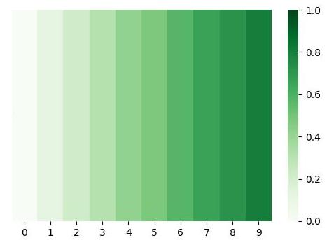
(a) Label distribution skew

(b) Feature distribution skew

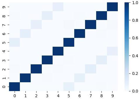
(c) Label concept skew

(d) Feature concept skew

Figure 2: Visualization of the cosine similarity matrix. Let $s$ denote the value of x-axis or y-axis in the figures. For the Figure. (a), $s$ indicates the number of the same label between these two clients. For the Figure. (b), we rotated the data with $36\times s$ degrees. For the Figure. (c), we modified the label $y=(y+s)$ mod $10$. For the Figure. (d), we use gradients calculated based on data samples from MNIST ($s\in[0,5)$) and Fashion-MNIST ($s\in[5,10)$). Then, we random initialize a linear model as anchor $\bm{\psi}$ for the digit recognition task. We calculate the representation $\Psi(\cdot)$ based on these partitioned datasets and observe the cosine similarity.

3.1 Preliminaries

The conventional CFL approach is to cluster clients with similar data distribution. Then, it aims to minimize the following objectives for each cluster $k\in[K]$:

$$\min_{\bm{\theta}_{1},...,\bm{\theta}_{K}}\mathbb{E}_{D^{(k)}\sim\mathcal{P}_{k}}[\ell(\bm{\theta}_{k};D^{(k)})],$$ (1)

s.t. $$\;\mathcal{C}=\{c_{1},\dots,c_{K}\},\;D^{(k)}=\cup_{i\in c_{k}}D_{i},$$

where $\mathcal{C}$ denotes client clustering results, and $D^{(k)}$ denotes the data samples of all clients in cluster $k$. The federated client clustering results, i.e., the subjective term in Equation (1), determines the performance of CFL to some extent. Therefore, Equation (1) motivates that the federated client clustering is a vital component in CFL.

We design a distribution extractor function $\Psi(D)=\texttt{Normalize(}\frac{\partial\ell(\bm{\psi};D)}{\partial\bm{\psi}}$), which indicates the updated direction toward the local minimum corresponding for the input dataset $D$, anchor model $\bm{\psi}$ and loss function $\ell$. We do not optimize the anchor model $\bm{\psi}$ and maintain the loss function $\ell$ constant across all datasets in our implementations. As a result, the $\Psi(\cdot)$ output can be viewed as a representation of data distribution corresponding to the input dataset. Based on the findings with Non-IID data (Zhao et al., 2018), we expect datasets with similar data distributions to provide similar $\Psi(\cdot)$ values. Then, we use cosine similarity to evaluate the distribution similarity of the two decentralized datasets, i.e., given any two unknown datasets $D_{i}$, $D_{j}$, the similarity is determined as:

$$\cos(\Psi(D_{i}),\Psi(D_{j}))=\frac{\Psi(D_{i})\cdot\Psi(D_{j})}{\|\Psi(D_{i})\|\|\Psi(D_{j})\|}.$$

To better support our assumptions, we implement observation experiments on cosine similarity, as shown in Figure 2, in which we augment MNIST/Fashion-MNIST dataset and partition them with varying levels of augmentation. The results reveal a significant difference in cosine similarity values. As a result, we conclude that $\Psi(\cdot)$ could represent a local data distribution, and clients with similar local data distributions (at both label and feature levels) have higher cosine similarity.

3.2 Stochastic Federated Client Clustering

Based on the observations, we implement a stochastic federated client clustering algorithm in this section. In detail, we aim to cluster federated clients by minimizing the following objective:

$$\min_{\mathcal{C}}\sum_{i=1}^{\tilde{K}}\sum_{j=i+1}^{\tilde{K}}\cos\big{(}\Psi(\tilde{D}^{(i)}),\Psi({\tilde{D}^{(j)}})\big{)},$$ (2)

where $\Psi({\tilde{D}^{(j)}})\triangleq\frac{1}{|c_{j}|}\sum_{i\in c_{j}}\Psi(D_{i})$ is the average point for decentralized local datasets of clients in the current $j$-th cluster in $\mathcal{C}$, $\tilde{K}$ denotes the number of clusters and $\tilde{K}=|\mathcal{C}|$. As the larger cosine similarity indicates the closer distance, minimizing the objective is to find the best partition $\mathcal{C}$ where the representations of current clusters are far from each other.

At the initialization stage of stochastic federated client clustering, we treat each client as a single cluster. In other words, the server maintains a partition set $\mathcal{C}=\{c_{1},c_{2},\dots,c_{N}\}$, where $N$ is the number of clients. For each $c_{i}\in\mathcal{C}$, we have $c_{i}=\{i\}$ and $i$ denotes the client id. Meanwhile, we have $\Psi(\tilde{D}^{(k)})=\Psi(D_{i})$ for all $k,i\in[N]$ and $\tilde{K}=N=|\mathcal{C}|$ at the beginning.

For the federated client clustering process, we greedily decrease the value of Equation (2) by merging the similar clusters sampled at each round. We adjust this merging process via a threshold $\tau$, indicating the minimum cosine similarity that two datasets should be considered similar. In practice, the Equation (2) can be represented by a pair-wise cosine similarity matrix $M$, where $M_{i,j}$ indicates the cosine similarity between the $i$-th and the $j$-th clusters in $\mathcal{C}$.

We summarise the stochastic federated client clustering procedure in Lines 4-13, Algorithm 1. For each federated round, the server would request the local data distribution representation from the sampled clients (Line 6). Then, the server updates the distribution representation of clusters (Line 9). Finally, the server merges any two clusters that satisfy the requirements (Lines 11-13). For each merging procedure, the current number of clusters $\tilde{K}$ is reduced by 1. If the federated server samples all clients at the first round, StoCFL recovers to client-wise agglomerative clustering, with the metric provided by distribution extractor $\Psi(\cdot)$.

3.3 Bi-level Clustered Federated Learning

In this section, we established a bi-level CFL objective to further improve conventional CFL approaches. Looking back to the conventional CFL objective in Equation (1), the cluster models are optimized within the cluster alone, with no inter-cluster knowledge sharing. Although the implicit data distribution may differ between clusters, we argue that there is certain knowledge that can be shared by one cluster model to better the other. Based on the observation, we propose the bi-level CFL objective, which regularizes the local optimization and improves cluster models via a shared global model.

In detail, corresponding with the client clustering procedure, the server maintains a global model denoted by $\bm{\omega}$ and cluster models $\bm{\theta}_{k},k\in[\tilde{K}]$. Our method solves a bi-level optimization problem for all cluster $k\in[\tilde{K}]$ given by:

$$\min_{\bm{\theta}_{k}}f_{k}(\bm{\theta}_{k})+\frac{\lambda}{2}\|\bm{\theta}_{k}-\bm{\omega}^{*}\|^{2},$$ (3)

$$s.t.\; \bm{\omega}^{*}\in\arg\min_{\bm{\omega}}G\big{(}f_{1}(\bm{\omega}),\dots,f_{N}(\bm{\omega})\big{)},$$

where $N$ is the total number of clients, $f_{i}(\cdot)=\mathbb{E}[\ell(\cdot;D_{i})]$ is empirical loss for the $i$-th client, and $G(\cdot)$ denotes the global objective function for the global model $\bm{\omega}$.

At the initialization stage, we make $\bm{\omega}_{0}=\bm{\theta}_{1}=\dots=\bm{\theta}_{N}$ and $\tilde{K}=N$. Meanwhile, if any two clusters are merged in the client clustering, then the server will merge corresponding cluster models. Hence, the real-time number of clusters $\tilde{K}$ is always the same as the number of cluster models.

The pseudocode of bi-level CFL is described in Lines 14-23, Algorithm 1. During the training process, the server broadcasts to sampled clients the global model $\bm{\omega}$ and corresponding cluster model $\bm{\theta}_{k}$. Then, the sampled clients perform several steps of SGD to optimize the cluster model (Line 21) and global model (Line 22) locally before uploading updated models to the server. The server updates the global model by aggregating the models from all sampled clients (Line 17). Then, the server updates the cluster models respectively (Lines 18-19).

3.4 Discussion

This section goes through the critical components that could affect the StoCFL. In particular, we discuss the impact of the global model on the cluster model. Additionally, we explain the clustering and optimization parameters to clarify the position of StoCFL in global FL and personalized FL.

Global model $\bm{\omega}$. In our bi-level optimization objective, the global model $\bm{\omega}$ fits the data samples of all clients. Hence, the global model preserves the knowledge (including distribution and feature information) of all clients. As a result, using the regularization term in local cluster model optimization, knowledge from separate clusters might be transferred to others. Additionally, the clustered learning process is separated from the global model optimization process. Hence, StoCFL is free to select the global objective $G(\cdot)$ (Li et al., 2021a). Consequently, the cluster model could inherit the convergence benefit (e.g., robustness or fairness).

Relation to clusters $\mathcal{C}$. The performance of cluster models is subjected to the client clustering results. Meanwhile, the client clustering results $\tilde{K},\mathcal{C}$ depend on the merging threshold $\tau$. Particularly, no clusters will be merged if $\tau=1$. Then, the final number of clusters will be $\tilde{K}=N$, which will degenerate the optimization objective function (3) to the personalized FL algorithm Ditto (Li et al., 2021a). If $\tau=-1$, however, all clients will be clustered together. As a result, the optimization objective degenerates to the global FL algorithm FedProx (Li et al., 2020b). Hence, by altering the clustering threshold $\tau$, the StoCFL could achieve an effective balance between global FL and personalized FL.

Regularization weight $\lambda$. The $\lambda$ is to adjust the impact of the global model on cluster models. When $\lambda$ is set to 0, the objective function degenerates into the conventional CFL task that is described in Equation (1). As the $\lambda$ grows large, it makes the cluster model reach the global objective function $G(\cdot)$. Furthermore, if $\lambda=0,\tau=-1$, StoCFL recovers to FedAvg. The impacts of $\lambda$ are further studied in Table 3, Section 4.3.

Input: Client set $S$, where $|S|=N$, initialized cluster partition $\mathcal{C}=\{c_{1},\dots,c_{N}\}$, initialized model $\bm{\omega}_{0},\bm{\theta}=[\bm{\theta}_{1},\dots,\bm{\theta}_{N}]$, anchor $\bm{\psi}$, threshold $\tau$ and learning rate $\eta$.

Output: Cluster result $\mathcal{C}=\{c_{1},\dots,c_{\tilde{K}}\}$, cluster models $\bm{\theta}_{1},\dots,\bm{\theta}_{\tilde{K}}$, and global model $\bm{\omega}$

1 ServerProcedure:

2        $P\leftarrow\emptyset$

3       for round $t$ $\in$ $[T]$ do

4               Random sample a subset of client $S^{t}\subseteq S,|S^{t}|=m$.

              // federated client clustering

5               for client id $i\in(S^{t}\cap\complement_{S}P)$ in parallel do

6                      $\Psi(D_{i})\leftarrow\textrm{GetDatasetRepresentation}(\bm{\psi})$

7              

8              $P\leftarrow P\cup S^{t}$

9              for $c_{k}\in\mathcal{C}$ do

10                      $\Psi(\tilde{D}^{(k)})=\sum_{i\in c_{k}}\Psi(D_{i})$

11              

12              Obtain cosine similarity matrix $M$ following Equation 2.

13              for $M_{i,j}$ in $M$ do

14                      if $M_{i,j}>\tau$ then

15                             $c_{i}\leftarrow c_{i}\cup c_{j},\mathcal{C}\leftarrow\mathcal{C}/c_{j}$

16                     

17              

              // clustered federated learning

18               for client id $i\in S^{t}$ in parallel do

19                      Let $k$ denote the index of the cluster and client id $i\in c_{k}$.

20                     $\bm{\omega}^{i}_{t},\theta_{k}^{i}\leftarrow\textrm{ClientProcedure}(\bm{\omega}_{t},\bm{\theta}_{k})$

21              $\bm{\omega}_{t+1}\leftarrow\textrm{Aggregate}([\bm{\omega}^{i}_{t}]),i\in S^{t}$

22              for $c_{k}\in C^{t}$ and indexed by $k$ do

23                      $\bm{\theta}_{k}\leftarrow\textrm{FedAvg}([\bm{\theta}_{k}^{i}]),i\in c_{k}$

24              

25       

26

27ClientProcedure($\bm{\omega},\bm{\theta}_{k}$):

28       

29       $\bm{\theta}_{k}^{i}\leftarrow\bm{\theta}_{k}-\eta\big{(}\nabla f_{i}(\bm{\theta}_{k})+\lambda(\bm{\theta}_{k}-\bm{\omega})\big{)}$

30       $\bm{\omega}^{i}\leftarrow\bm{\omega}-\eta\nabla f_{i}(\bm{\omega})$

31       return $\bm{\omega}^{i},\bm{\theta}_{k}^{i}$

Algorithm 1 Stochastic Clustered Federated Learning

4 Experiment Evaluation

In this part, we assess the performance of StoCFL using four basic Non-IID settings and the real-world dataset FEMNIST. Our experiment investigation includes federated client clustering and CFL evaluation. Furthermore, we discuss the effect of StoCFL hyper-parameters. In the end, we demonstrate the application inference ability of StoCFL and study its generalization ability to unseen clients. The experiment is developed using the open-source FL framework (Zeng et al., 2021).

4.1 Stochastic Client Clustering with Non-IID Data

We evaluate the stochastic federated client clustering algorithm on the MNIST (LeCun et al., 1998) and Fashion-MNIST (Li et al., 2021b). We recall that the MNIST/Fashion-MNIST dataset has 60,000 training samples and 10,000 test samples with ten classes. To simulate an FL environment where the data distributions among clients are different, we augment and partition these datasets as follows.

• Pathological MNIST (McMahan et al., 2017): we sort the data samples by labels and split them into {{0,1,2},{3,4},{5,6},{7,8,9}} (4 clusters). Then we randomly partition the dataset into 100 clients for each cluster, resulting in 400 clients with $K=4$. We refer to it as Label distribution skew.

• Rotated MNIST (Lopez-Paz and Ranzato, 2017): we augment MNIST by rotating images with 0, 90, 180, and 270 degrees, resulting in $K=4$ clusters. We randomly partition the Rotated MNIST of each degree into 100 clients. This scenario is Feature distribution skew.

• Shifted MNIST (Sattler et al., 2020a): we modify the label of each sample by adding shift level $s$(i.e., $\bar{y}_{s}=(y+s)\%10,s\in{0,3,6,9}$) and partition dataset of each shift level into 100 clients. Hence, this case shall be Label concept skew.

• Hybrid MNIST: we partition MNIST and Fashion-MNIST into 100 clients, resulting in 200 clients and 2 clusters. The label across clients is the same ($y\in[10]$), but the feature domain is different. Therefore, this case is Feature concept skew.

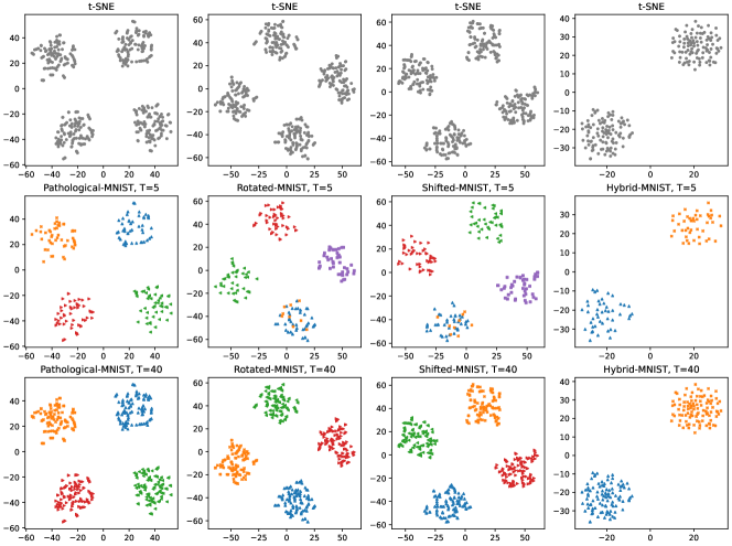
(a) Visualization of clustering

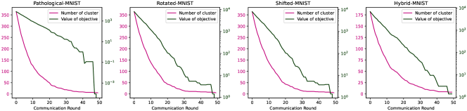
(b) Clustering status curve

Figure 3: Illustration of client clustering. In Figure (a), the first row is the t-SNE results on all $[\Psi(D_{i})],i\in[N]$, where each point denotes the data distribution of the dataset from each client. The other row is the clusters at communication round $T=\{5,10,40\}$, which are colored by StoCFL. In Figure (b), we depicted the overall number of clusters and the value of the clustering objective in Equation 2 at each communication round.

In experiments, we randomly initialize an anchor model $\psi$ and choose the cross-entropy loss as $\ell$ for the classification task. Based on that, we obtain all representation vectors using $\Psi(\cdot)$ and display them using t-SNE (Van der Maaten and Hinton, 2008) visualizing. We conducted 50 rounds of the proposed stochastic federated client clustering procedure, where only 10% of clients are randomly sampled each round. The visualization results are shown in Figure 3(a). The graph with grey points depicts the visualization results of distribution representation vectors. Furthermore, clear clusters are shown from the representation vectors captured by t-SNE, which further proves that $\Psi(\cdot)$ could extract and represent the local data distributions. Besides, an additional clustering status curve is depicted in Figure 3(b). The client clustering results demonstrate that our federated client clustering could deal with different Non-IID scenarios. Based on the distribution representation technique, we could establish a promising CFL method.

Table 1: Test accuacies(%)$\pm$ std.

	Rotated MNIST, K=4						Rotated CIFAR, K=2
$N$, $|D|$	4800, 50		2400, 100		1200, 200		200, 500
Sample Rate	10%	100%	10%	100%	10%	100%	10%	100%
FedAvg	95.72$\pm$0.13	96.10$\pm$1.26	95.32$\pm$0.16	96.00$\pm$1.31	94.96$\pm$0.11	95.72$\pm$1.60	48.26$\pm$0.66	47.98$\pm$1.73
FedProx	76.45$\pm$0.07	76.47$\pm$0.08	77.40$\pm$0.09	77.48$\pm$0.08	77.82$\pm$0.07	77.90$\pm$0.09	47.17$\pm$0.35	47.15$\pm$0.36
Ditto	65.05$\pm$0.05	73.60$\pm$0.05	73.93$\pm$0.11	79.71$\pm$0.05	79.38$\pm$0.08	83.96$\pm$0.03	46.91$\pm$0.38	46.61$\pm$0.39
IFCA $\tilde{M}$=2	84.42$\pm$1.05	84.98$\pm$0.28	85.25$\pm$0.94	84.64$\pm$2.54	86.12$\pm$0.78	84.37$\pm$4.40	50.62$\pm$1.86	49.83$\pm$2.79
IFCA $\tilde{M}$=4	91.74$\pm$0.02	90.43$\pm$2.71	91.39$\pm$1.24	90.75$\pm$2.48	91.00$\pm$1.44	88.69$\pm$2.83	50.80$\pm$1.69	51.40$\pm$2.00
IFCA $\tilde{M}$=6	91.74$\pm$0.03	91.65$\pm$0.12	91.94$\pm$0.13	91.99$\pm$0.04	92.15$\pm$0.07	92.17$\pm$0.04	51.04$\pm$0.40	50.63$\pm$1.85
StoCFL	97.00$\pm$0.04	97.36$\pm$0.38	96.89$\pm$0.02	97.4$\pm$0.35	96.71$\pm$0.04	97.40$\pm$0.38	52.84$\pm$0.74	54.99$\pm$0.66

4.2 Clustered Federated Learning

Baselines. We compare the IFCA (Ghosh et al., 2020) and CFL (Sattler et al., 2020a) under different Non-IID settings. Before that, we first recall the details of the CFL techniques. IFCA (Ghosh et al., 2020) takes an input of the assumption number of cluster $\tilde{M}$. Then, the server initializes $\tilde{M}$ different models for each cluster and broadcasts them to clients for each round. The clients will optimize the specific model, which achieves the lowest forward loss on the local dataset. Clients upload the updated model to the server. The server would aggregate the updated $\tilde{M}$ models in the same cluster following FedAvg. CFL (Sattler et al., 2020a) monitors the model updates of all clients for each round. In the beginning, all clients are in the same cluster. Then, the server will bi-partition clients into two clusters when certain conditions are satisfied. Particularly, The CFL server would recursively run the above procedures in the same cluster till the partition conditions are no longer satisfied (client clustering finished).

Settings. We compare the baseline algorithms respectively using identical experimental conditions as described in their study. The MNIST task model is a linear classification model with a hidden layer of 2048 units, and the CIFAR10 task model is a convolution neural network model with two convolutional layers followed by two fully connected layers. We execute five runs for each experiment, each with a different random seed. We also provide the average test accuracy and standard deviation. Without loss of generality, we initialize model $\bm{\psi}=\bm{\omega}_{0}$ for the distribution extractor function $\Psi(\cdot)$ in experiments, and the loss function $\ell$ is the cross-entropy loss for the classification task. As experiments are conducted with multiple random seeds, we argue that the distribution extractor $\Psi(\cdot)$ is robust to the model initialization.

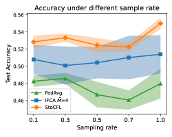
Figure 4: Robustness comparison of different federated learning methods with various sampling rates.

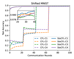
Figure 5: Evolution curves of test accuracy for CFL and StoCFL with increasing communication rounds.

Experiments in IFCA setting. Following the setting of IFCA, we create the Rotated MNIST and Rotated CIFAR10 datasets. Firstly, We rotated the MNIST data samples by 0, 90, 180, and 270 degrees, resulting in cluster number $K=4$. Then, we randomly partition datasets into $N=(4800,2400,1200)$ clients, and each client has $|D|=(50,100,200)$ data samples. For the configuration of MNIST tasks, We run 100 federated communication rounds for the Rotated MNIST setting. Each client performs 5 epochs of local SGD with full batch size and the learning rate $\eta=0.1$. Besides, the Rotated CIFAR10 is created similarly with 0 and 180 degrees of rotation. We run 200 federated communication rounds for the Rotated CIFAR setting. Each client performs 5 epochs of local SGD with a local batch size is 50 and the learning rate $\eta=0.1$. For the hyper-parameters of StoCFL, the stochastic client clustering threshold $\tau=0.5$, and the optimization parameter $\lambda=0.05$.

We highlight that the original experiments in IFCA report a full client sample rate in MNIST and a client sample rate of 10% in CIFAR10. For a fair comparison, we choose different sample rates for both MNIST and CIFAR10 tasks. In addition, we compare to FedAvg, FedProx, and Ditto to demonstrate the improvement of StoCFL. The performance results are shown in Table 1. According to the results, StoCFL outperforms IFCA in most cases. The global baseline performance is worse since the global model tries to fit all data samples from all distributions. More importantly, we observe that IFCA fails to cluster clients from different data distributions in MNIST experiments, where a particular model may dominate another model from the beginning. That is, if a model fits two distributions well in the first few rounds, then this model will dominate another model, making it no chance to fit the expected distribution (no clients will update this model). Hence, we argue that IFCA depends on model initialization to some extent. Meanwhile, previous studies (Wu et al., 2022; Ma et al., 2022) on the heterogeneity of FL observe a similar phenomenon in the IFCA algorithm.

We study the effect of client sample rate on StoCFL with the Rotated CIFAR10 setting, where the results are depicted in Figure 5. The performance curve of StoCFL is stable and better with different settings of the sample rate. Hence, the results reveal that StoCFL is robust and flexible with the proportion of client participation.

Experiments in CFL setting. Following the setting of CFL, we conduct experiments on the Shifted MNIST and the Shifted CIFAR-10 dataset (Krizhevsky et al., 2009). In this case, datasets are partitioned into $N=20$ clients, each belonging to one of $K=4$ clusters. The labels of each client data are modified by randomly shifted labels, i.e., $\tilde{y}=(y+s)\%10,s\in\{0,3,6,9\}$. For a fair comparison, we let all clients participate in StoCFL in this part. Additionally, we also conduct IFCA on this setting for comparison. The performance is shown in Table 7. We obtain a close model performance in the setting of CFL, however, the accuracy curve of StoCFL is better in most training rounds (shown in Figure 5). Besides, the CFL requires full client participation for every round to bi-partition the clients at a proper stage. In contrast, StoCFL supports an arbitrary proportion of client participation, which reveals the flexibility of StoCFL.

Figure 6: Test accuracy(%)$\pm$ std

	Shifted MNIST	Shifted CIFAR
$N$, $|D|$	20, 9600	20, 8000
FedAvg	24.44$\pm$0.03	13.01$\pm$2.48
IFCA	98.11$\pm$0.03	54.05$\pm$0.59
CFL	98.20$\pm$0.02	55.23$\pm$1.02
StoCFL	98.14$\pm$0.01	55.42$\pm$1.42

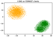
Figure 7: Clustering Results of StoCFL on FEMNIST.

Real-world dataset evaluation. We provide the additional experimental results on the real-world dataset FEMNIST (Cohen et al., 2017), which is proposed by LEAF (Caldas et al., 2018). It is a realistic FL dataset where the data samples on a single client are the handwritten digits or letters from a specific writer. Besides, There are 3,597 clients in FEMNIST, and the number of data samples among these clients is different. Hence, this setting could be considered a hybrid Non-IID scenario. Although there are no clear clusters for FEMNIST clients, the writing style of different people may be clustered. For the model, we use a neural network with two convolutional layers, with a max pooling layer after the convolutional layer, followed by two fully connected layers. We also added a dropout ratio of 0.5 between the convolutional layer and the fully connected layer. The network parameters initialization follows Xavier (Glorot and Bengio, 2010). We run 100 rounds of FL with $5\%$ clients sampled per round. We also evaluate IFCA and CFL on FEMNIST for comparison. The final results on FEMNIST are reported in Table 2.

The results indicate that StoCFL achieves better performance on FEMNIST, compared with IFCA and CFL. Furthermore, we highlight that CFL consumes more resources as it requires the full participation of clients. For the client clustering results, we observe that StoCFL clusters FEMNIST clients into two main clusters (shown in Figure 7), i.e., FEMNIST consists of two implicit data-generating distributions. Importantly, previous studies (Marfoq et al., 2021; Ghosh et al., 2020) on FEMNIST draw the same conclusion, which proves the StoCFL correct. In all, the real-world dataset evaluation results reveal the ability of StoCFL to handle non-synthetic datasets, and further indicate the practical value of StoCFL.

Table 2: Test accuracy(%)$\pm$ std on FEMNIST.

IFCA	$\tilde{M}$=2	$\tilde{M}$=3	CFL	FedAvg
	73.11$\pm$0.92	69.11$\pm$2.49	79.64$\pm$0.37	86.27$\pm$0.11

StoCFL	$\tau$=0.55	$\tau$=0.60	$\tau$=0.65
	90.92$\pm$0.02	90.71$\pm$0.04	90.23$\pm$0.20

4.3 Impact of Hyper-parameters

In this section, we first study the influence of regularization weight $\lambda$ on model performance. Then, we illustrate the impacts of clustering threshold $\tau$ on clustering results. Based on the results, we provide insights about the tuning of hyper-parameters when deploying StoCFL on applications.

Effect of $\lambda$. We demonstrate the effect of $\lambda$ via experiments on Pathological-MNIST, Rotated-MNIST, Shifted-MNIST, and Hybrid-MNIST settings. We run 50 communication rounds of StoCFL with $\lambda=\{0,0.01,0.05,0.5,1,10\}$, and report the test accuracy of the global model and cluster models. The global accuracy is the performance of the final $\bm{\omega}$ on all augmented test sets, while the contents of other columns are the average performance of cluster models. The results are summarized in Table 3.

We note that $\lambda=0$ indicates the conventional CFL with correct client clustering results. In comparison, the results with $\lambda>0$ prove that StoCFL improves the cluster model’s performance by introducing useful knowledge from other clusters via the regularization term. For instance, the global accuracy results of Rotated-MNIST and Shifted-MNIST are distinct, while the cluster models are enhanced by the regularization term with $\lambda=0.05$. Besides, compared with the conventional CFL results ($\lambda=0$), the results of StoCFL are better.

Furthermore, given the impacts of decentralized data distributions in these four settings are different, the value of $\lambda$ where the cluster models achieve the best accuracy is not the same. Hence, we conclude that the best $\lambda$ relies on the real scenario of Non-IID data. In the real-world training process of StoCFL, the $\lambda$ could be adjusted dynamically during the training process. Besides, we could refer to  (Li et al., 2020b, 2021a) for the best strategies for choosing $\lambda$. We will further study the relation between $\lambda$ and the Non-IID data in future work.

Table 3: Effect of $\lambda$. Test accuracy (%).

MNIST	Global	StoCFL, $\lambda$
		10	1	0.5	0.05	0.01	0
Pathological	92.17	89.28	86.89	83.49	37.83	24.12	24.05
Rotated	92.65	62.06	94.88	95.28	95.86	94.20	92.25
Shifted	24.46	32.69	92.36	93.85	95.12	93.80	92.22
Hybrid	92.50	92.26	92.75	92.77	92.69	91.99	90.11

Effect of $\tau$. We demonstrate the effects of $\tau$ on client clustering with a hybrid Non-IID setting combination. In this part, we follow the partition strategies described in Section 4.1. Firstly, we create Rotate-MNIST by 0,180 degrees of rotation and marked them with R0, R180. Then, we pathologically partition (marked by P1, P2, P3, P4) each of them into 200 clients. In this case, we have 400 clients in total, where the client data distributions are 2 clusters in feature distribution (rotation degree), and 4 clusters in label distribution. From the overall perspective, there are 8 clusters in both label and feature distribution. We conduct the stochastic federated client clustering procedure with different $\tau$ on this setting. In our experiments, we observe that the clustering results vary with the value of $\tau$. Then, we depict the representative results via t-SNE in Figure 8 and color the points according to the clustering results.

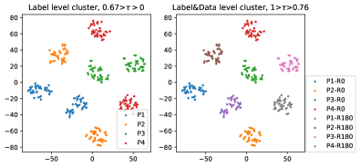
Figure 8: The value of $\tau$ decides the clustering focus.

The results indicate that the value $\tau$ determines the focus of the clustering algorithm. For instance, $\tau>0.76$ in this case, the clustering algorithm will cluster clients only when their feature distribution and label distribution are similar. In contrast, $\tau<0.67$ makes the clustering algorithm focus on the label distribution while ignoring the differences in feature level. Hence, a higher value of $\tau$ decides the client clustering in a more fine-grained way. More importantly, we emphasize that StoCFL is robust to the client clustering results as shown in Table 2. For a further relation between the clustering granularity and the threshold $\tau$, we will study it in future work.

4.4 Cluster Inference and Generalization

In this section, we further explain the advantages of StoCFL for practical applications. First, we demonstrate the ability of StoCFL to infer newly joined clients, which reveals that StoCFL could handle a varying FL system. Based on the inference ability, we further study the generalization performance of StoCFL in the FEMNIST setting.

Cluster inference for newly joined clients. StoCFL is flexible with newly joined clients. In other words, the StoCFL server could determine which cluster to join for a new coming client. Furthermore, StoCFL is adaptable in terms of inferring a newly joined client during or after the training process. Consider a newly joined client with a local dataset $\hat{D}$ that reports the local representation $\Psi(\hat{D})$ to the server. Then, the server could then use a few steps to determine the target cluster:

1. Calculate the candidate cluster with the closest distance

   $$\hat{d}=\arg\max\text{cos}(\Psi(\hat{D}),\Psi(\tilde{D}^{(j)})),\;j\in[\tilde{K}],$$

   and record the candidate cluster id $\hat{c}$.

2. If $\hat{d}\geq\tau$, then assign the client to the cluster $\hat{c}$. Otherwise, the server assigns the client to a new cluster marked by $\tilde{K}+1$, $\tilde{K}=\tilde{K}+1$, and let $\theta_{\tilde{K}}=\theta_{\hat{c}}$.

We emphasize that if the client is unable to join any existing cluster, the server should assign a cluster model with the closest cluster distribution. As a result, the cluster model could be learned from good initialization during the training process. Furthermore, once the FL training process is finished, we could use the closest model to predict data samples from new clients.

Table 4: Generalization performance (%) on FEMNIST

Method	FedAvg	CFL	IFCA	StoCFL
Test Accuracy	85.93$\pm$0.16	79.78$\pm$0.28	74.82$\pm$0.49	91.00$\pm$0.05
Unparticipation	86.70$\pm$0.22	73.24$\pm$0.99	75.78$\pm$0.45	91.06$\pm$0.05

Generalization to unseen clients. The experiments in this section are carried out in the FEMNIST environment in order to evaluate the generalization performance of cluster models. In particular, 1,079 clients (30%) were selected as test clients who did not participate in the FL process. Only 2,518 clients (70%) are participating in the CFL process in this case. Then, using this configuration, we run StoCFL, CFL, and IFCA to infer the cluster of unparticipated clients using their training data samples. As a result, we report in Table 4 the accuracy of test data samples from participated and unanticipated clients. According to the results, StoCFL achieves better generalization performance while preserving higher test accuracy.

5 Conclusion and Future Work

In this paper, we proposed a novel CFL algorithm StoCFL, which consists of stochastic client clustering and bi-level CFL algorithms. Our study demonstrates that StoCFL could cluster federated clients with different unknown distributions and train better-generalized models. Besides, StoCFL is flexible and robust with real-world applications, especially in a varying FL system. Furthermore, the results of intensive experiments have shown the superiority of the proposed algorithms.

For future work, we plan to improve the framework from algorithm and system aspects. For instance, the global model in bi-level optimization can be replaced by different model architectures. Then, we can combine knowledge transfer techniques in local optimization for better cluster models. Besides, we will establish a dynamic join-leave mechanism to deal with a scenario where the local data samples are changing. Furthermore, such a dynamic-join-leave mechanism could exclude potential Byzantine clients from a benign cluster and obtain more robust results in federated learning.

References

- McMahan et al. (2017) Brendan McMahan, Eider Moore, Daniel Ramage, Seth Hampson, and Blaise Aguera y Arcas. Communication-efficient learning of deep networks from decentralized data. In Artificial intelligence and statistics, pages 1273–1282. PMLR, 2017.
- Yang et al. (2019) Qiang Yang, Yang Liu, Tianjian Chen, and Yongxin Tong. Federated machine learning: Concept and applications. ACM Transactions on Intelligent Systems and Technology (TIST), 10(2):1–19, 2019.
- Zhao et al. (2018) Yue Zhao, Meng Li, Liangzhen Lai, Naveen Suda, Damon Civin, and Vikas Chandra. Federated learning with non-iid data. arXiv preprint arXiv:1806.00582, 2018.
- Li et al. (2020a) Tian Li, Anit Kumar Sahu, Manzil Zaheer, Maziar Sanjabi, Ameet Talwalkar, and Virginia Smith. Federated optimization in heterogeneous networks. In Inderjit S. Dhillon, Dimitris S. Papailiopoulos, and Vivienne Sze, editors, Proceedings of Machine Learning and Systems 2020, MLSys 2020, Austin, TX, USA, March 2-4, 2020. mlsys.org, 2020a.
- Li et al. (2022) Zonghang Li, Yihong He, Hongfang Yu, Jiawen Kang, Xiaoping Li, Zenglin Xu, and Dusit Niyato. Data heterogeneity-robust federated learning via group client selection in industrial iot. IEEE Internet Things J., 9(18):17844–17857, 2022.
- Zeng et al. (2022a) Shenglai Zeng, Zonghang Li, Hongfang Yu, Yihong He, Zenglin Xu, Dusit Niyato, and Han Yu. Heterogeneous federated learning via grouped sequential-to-parallel training. In Database Systems for Advanced Applications - 27th International Conference, DASFAA 2022, Virtual Event, April 11-14, 2022, Proceedings, Part II, volume 13246 of Lecture Notes in Computer Science, pages 455–471. Springer, 2022a.
- Sattler et al. (2020a) Felix Sattler, Klaus-Robert Müller, and Wojciech Samek. Clustered federated learning: Model-agnostic distributed multitask optimization under privacy constraints. IEEE transactions on neural networks and learning systems, 32(8):3710–3722, 2020a.
- Sattler et al. (2020b) Felix Sattler, Klaus-Robert Müller, Thomas Wiegand, and Wojciech Samek. On the byzantine robustness of clustered federated learning. In ICASSP 2020-2020 IEEE International Conference on Acoustics, Speech and Signal Processing (ICASSP), pages 8861–8865. IEEE, 2020b.
- Ghosh et al. (2020) Avishek Ghosh, Jichan Chung, Dong Yin, and Kannan Ramchandran. An efficient framework for clustered federated learning. Advances in Neural Information Processing Systems, 33:19586–19597, 2020.
- Briggs et al. (2020) Christopher Briggs, Zhong Fan, and Peter Andras. Federated learning with hierarchical clustering of local updates to improve training on non-iid data. In 2020 International Joint Conference on Neural Networks (IJCNN), pages 1–9. IEEE, 2020.
- Duan et al. (2021) Moming Duan, Duo Liu, Xinyuan Ji, Yu Wu, Liang Liang, Xianzhang Chen, Yujuan Tan, and Ao Ren. Flexible clustered federated learning for client-level data distribution shift. IEEE Transactions on Parallel and Distributed Systems, 2021.
- Ma et al. (2022) Jie Ma, Guodong Long, Tianyi Zhou, Jing Jiang, and Chengqi Zhang. On the convergence of clustered federated learning. arXiv preprint arXiv:2202.06187, 2022.
- Stallmann and Wilbik (2022) Morris Stallmann and Anna Wilbik. Towards federated clustering: A federated fuzzy -means algorithm (ffcm). arXiv preprint arXiv:2201.07316, 2022.
- Wang et al. (2022) Yi Wang, Mengshuo Jia, Ning Gao, Leandro Von Krannichfeldt, Mingyang Sun, and Gabriela Hug. Federated clustering for electricity consumption pattern extraction. IEEE Transactions on Smart Grid, 13(3):2425–2439, 2022.
- Mansour et al. (2020) Yishay Mansour, Mehryar Mohri, Jae Ro, and Ananda Theertha Suresh. Three approaches for personalization with applications to federated learning. arXiv preprint arXiv:2002.10619, 2020.
- Hsieh et al. (2020) Kevin Hsieh, Amar Phanishayee, Onur Mutlu, and Phillip Gibbons. The non-iid data quagmire of decentralized machine learning. In International Conference on Machine Learning, pages 4387–4398. PMLR, 2020.
- Li et al. (2020b) Tian Li, Anit Kumar Sahu, Manzil Zaheer, Maziar Sanjabi, Ameet Talwalkar, and Virginia Smith. Federated optimization in heterogeneous networks. Proceedings of Machine Learning and Systems, 2:429–450, 2020b.
- Acar et al. (2021) Durmus Alp Emre Acar, Yue Zhao, Ramon Matas Navarro, Matthew Mattina, Paul N. Whatmough, and Venkatesh Saligrama. Federated learning based on dynamic regularization. In 9th International Conference on Learning Representations, ICLR 2021, Virtual Event, Austria, May 3-7, 2021. OpenReview.net, 2021.
- Oh et al. (2022) Jaehoon Oh, SangMook Kim, and Se-Young Yun. FedBABU: Toward enhanced representation for federated image classification. In International Conference on Learning Representations, 2022.
- Zeng et al. (2022b) Dun Zeng, Shiyu Liu, Siqi Liang, Zonghang Li, and Zenglin Xu. Aggregating gradients in encoded domain for federated learning. CoRR, abs/2205.13216, 2022b.
- Li et al. (2021a) Tian Li, Shengyuan Hu, Ahmad Beirami, and Virginia Smith. Ditto: Fair and robust federated learning through personalization. In International Conference on Machine Learning, pages 6357–6368. PMLR, 2021a.
- Marfoq et al. (2021) Othmane Marfoq, Giovanni Neglia, Aurélien Bellet, Laetitia Kameni, and Richard Vidal. Federated multi-task learning under a mixture of distributions. Advances in Neural Information Processing Systems, 34:15434–15447, 2021.
- T Dinh et al. (2020) Canh T Dinh, Nguyen Tran, and Josh Nguyen. Personalized federated learning with moreau envelopes. Advances in Neural Information Processing Systems, 33:21394–21405, 2020.
- Pedrycz (2021) Witold Pedrycz. Federated fcm: Clustering under privacy requirements. IEEE Transactions on Fuzzy Systems, 2021.
- Xie et al. (2020) Ming Xie, Guodong Long, Tao Shen, Tianyi Zhou, Xianzhi Wang, Jing Jiang, and Chengqi Zhang. Multi-center federated learning. arXiv preprint arXiv:2005.01026, 2020.
- Zeng et al. (2021) Dun Zeng, Siqi Liang, Xiangjing Hu, and Zenglin Xu. Fedlab: A flexible federated learning framework. arXiv preprint arXiv:2107.11621, 2021.
- LeCun et al. (1998) Yann LeCun, Léon Bottou, Yoshua Bengio, and Patrick Haffner. Gradient-based learning applied to document recognition. Proceedings of the IEEE, 86(11):2278–2324, 1998.
- Li et al. (2021b) Qinbin Li, Yiqun Diao, Quan Chen, and Bingsheng He. Federated learning on non-iid data silos: An experimental study. arXiv preprint arXiv:2102.02079, 2021b.
- Lopez-Paz and Ranzato (2017) David Lopez-Paz and Marc’Aurelio Ranzato. Gradient episodic memory for continual learning. Advances in neural information processing systems, 30, 2017.
- Van der Maaten and Hinton (2008) Laurens Van der Maaten and Geoffrey Hinton. Visualizing data using t-sne. Journal of machine learning research, 9(11), 2008.
- Wu et al. (2022) Shanshan Wu, Tian Li, Zachary Charles, Yu Xiao, Ziyu Liu, Zheng Xu, and Virginia Smith. Motley: Benchmarking heterogeneity and personalization in federated learning. arXiv preprint arXiv:2206.09262, 2022.
- Krizhevsky et al. (2009) Alex Krizhevsky, Geoffrey Hinton, et al. Learning multiple layers of features from tiny images. 2009.
- Cohen et al. (2017) Gregory Cohen, Saeed Afshar, Jonathan Tapson, and Andre Van Schaik. Emnist: Extending mnist to handwritten letters. In 2017 international joint conference on neural networks (IJCNN), pages 2921–2926. IEEE, 2017.
- Caldas et al. (2018) Sebastian Caldas, Sai Meher Karthik Duddu, Peter Wu, Tian Li, Jakub Konečnỳ, H Brendan McMahan, Virginia Smith, and Ameet Talwalkar. Leaf: A benchmark for federated settings. arXiv preprint arXiv:1812.01097, 2018.
- Glorot and Bengio (2010) Xavier Glorot and Yoshua Bengio. Understanding the difficulty of training deep feedforward neural networks. In Proceedings of the thirteenth international conference on artificial intelligence and statistics, pages 249–256. JMLR Workshop and Conference Proceedings, 2010.