Comparison of High-Dimensional Bayesian Optimization Algorithms on BBOB

Abstract.

Bayesian Optimization (BO) is a class of black-box, surrogate-based heuristics that can efficiently optimize problems that are expensive to evaluate, and hence only small evaluation budgets are allowed. BO is particularly popular for solving numerical optimization problems in industry, where the evaluation of objective functions often relies on time-consuming simulations or physical experiments. However, many industrial problems depend on a large number of parameters. This poses a challenge for BO algorithms, whose performance is often reported to suffer when the dimension grows beyond 15 variables. Although many new algorithms have been proposed to address this problem, it is not well understood which one is the best for which optimization scenario.

In this work, we compare five state-of-the-art high-dimensional BO algorithms with vanilla BO and CMA-ES on the 24 BBOB functions of the COCO environment at increasing dimensionality, ranging from 10 to 60 variables. Our results confirm the superiority of BO over CMA-ES for limited evaluation budgets and suggest that the most promising approach to improve BO is the use of trust regions. However, we also observe significant performance differences for different function landscapes and budget exploitation phases, indicating improvement potential, e.g., through hybridization of algorithmic components.

1. Introduction

In countless areas of science, engineering, and beyond, researchers and developers deal with free parameters that can be tuned to achieve a specific goal. With the increase in computing power and simulation methods, optimization techniques have become always more popular in industry. They are replacing the manual trial-and-error method for parameter tuning, which is highly dependent on prior knowledge and expertise about the particular research area and subject, and which requires many trials before a satisfactory parameter configuration is found, without any guarantee of its optimality. In many application areas such as machine learning, neural network design, robotics, aerospace, and mechanical design, optimization deals with black-box problems, i.e., problems where the structure of the objective function, its derivatives, and/or the constraints is unknown, unexploitable, or non-existent. This is the case, for example, in design and prototyping processes, where engineers simulate the performance of new products with increasingly accurate numerical models and simulations. This makes evaluating a particular parameter setting extremely costly, reducing the affordable budget for simulations and making it impossible to fully explore the design space. When limited evaluation budgets are available in optimization, it is a common practice to rely on surrogate models, i.e., approximations that mimic the behavior of the expensive and unknown objective function to be optimized while being computationally cheaper to evaluate.

One of the most commonly used surrogate-based optimization methods is Bayesian Optimization (BO) (Mockus, 2012; Garnett, 2023). Through careful modeling based on Gaussian process regression (GPR) and intelligent search for candidate solutions through the optimization of an acquisition function, BO algorithms can deliver impressive optimization performance even with small evaluation budgets (Garnett, 2023). The potential of BO has been demonstrated in hundreds of studies across a wide range of domains, such as chemistry and material science (Hernández-Lobato et al., 2017; Griffiths and Hernández-Lobato, 2020; Kotthoff et al., 2021), biology, engineering and design (Lam et al., 2018; Raponi et al., 2019, 2021), robotics (Martinez-Cantin et al., 2009; Calandra et al., 2016; Junge et al., 2020), algorithm configuration (Hutter et al., 2011), hyperparameter tuning (Klein et al., 2017; Nguyen, 2019; Turner et al., 2021), and automated machine learning (Malkomes et al., 2016; Jin et al., 2019). However, when the dimensionality of the problem exceeds 15 variables, the performance of BO deteriorates due to the so-called curse of dimensionality (Bellman, 1966). Scaling BO to high-dimensional spaces is challenging as its statistical and computational complexity increases with dimension: the number of points queried to satisfactorily cover the search space increases exponentially with dimension, and optimizing the acquisition function requires more and more computational power, being a non-convex optimization problem on the same design space itself.

Related work: In recent years, characterized by increasingly complex systems and large and high-dimensional data, great efforts have been made to extend BO to higher dimensions, and various strategies have been proposed. According to (Binois and Wycoff, 2022), these are mainly based on (but not limited to) one of the following methods: Variable selection, additive models, linear and nonlinear embeddings, and trust regions. All of these strategies have advantages and disadvantages (see Figure 1), and it is not clear which one is best for which optimization scenario. In Section 2.1 we discuss these categories further and give some examples. However, for a more comprehensive overview, we refer the reader to available surveys on this topic (Malu et al., 2021; Binois and Wycoff, 2022), even though they are purely informative and lack an experimental study comparing the methods. On the other hand, comparative studies have been conducted to present new algorithms such as SMAC (Hutter et al., 2013), REMBO (Wang et al., 2016), TuRBO (Eriksson et al., 2019), SAASBO (Eriksson and Jankowiak, 2021), etc., but they are either outdated or limited to showing the potential of the proposed algorithm rather than presenting a comprehensive and unbiased performance comparison. Our work aims at filling this gap.

Disclaimer: In line with (Binois and Wycoff, 2022) we refer to the setting with dimension 60 as high-dimensional, even if BO-approaches for problems with several thousands of variables have been studied (Wang et al., 2016).

Our contribution: In this article we present the results of a benchmarking study that follows the standardized, well-established guidelines for unbiased performance comparison in numerical black-box optimization. With the goal to obtain a first overview over which high-dimensional BO (HDBO) approaches to favor for which problem characteristics, we benchmark five BO variants that are specifically designed for high-dimensional, low-budget optimization problems. We also include in our comparison two standard solvers, vanilla BO (Pedregosa et al., 2011) and the Covariance Matrix Adaptation Evolution Strategy (CMA-ES) (Hansen and Ostermeier, 2001). To obtain interpretable results, we focus on the 24 functions of (noiseless) the Black-Box Optimization Benchmarking (BBOB) suite from the COCO environment (Hansen et al., 2021) and compare algorithm performance for what we consider small evaluation budgets; motivated by our target applications in structural mechanics, we set the budget to $10D+50$. Key findings from our experiments are that (1) Vanilla BO performs better than CMA-ES for small dimensions and low budget, (2) many of the algorithms that aim to scale BO to high-dimensional spaces outperform vanilla BO and CMA-ES, with the convergence gap widening as the dimension increases, and (3) among the compared algorithms, the BO variant using trust regions performs particularly well on a large number of function, dimension, and budget combinations.

Reproducibility: Our code for reproducing the experiments is available on GitHub, in the public repository IOH-HDBO-Comparison. The project data is also available for interactive analysis and visualization on the IOHanalyzer platform (Wang et al., 2022) as ‘HDBO’ dataset. Code and full data obtained in the experiments are stored in Zenodo under the name of Comparison of High-Dimensional Bayesian Optimization Algorithms on BBOB..

The remainder of this paper is structured as follows: Section 2 introduces the BO algorithm and discusses various approaches specifically designed to tackle the issue of low performance in high-dimensional problems. Following this, Section 3 presents an overview of the experimental setup employed for our comparative study. Results are presented and discussed in Section 4 and Section 5. Finally, Section 6 summarizes the conclusions drawn from our study and outlines the subsequent important steps for further exploration of the current challenges. Additional details regarding the individual algorithms and an extensive analysis of the obtained results can be found in the appendix at the end of the paper.

2. Bayesian Optimization

Bayesian Optimization (Mockus, 2012; Frazier, 2018; Garnett, 2023) is one of the most widely used surrogate-based optimization algorithms. It is a global optimization strategy based on Bayesian inference, tailored to solve optimization problems with a small number of function evaluations.

BO involves two main components: a method for statistical inference, usually a GPR model, and an acquisition function that determines the optimal locations for sampling new points.

The procedure starts with a prior probability distribution for the objective function $f$, usually a Gaussian process prior, and a budget $T$ for the maximum number of function evaluations. Next, the objective function f is evaluated on $n_{0}$ points that are distributed within the design space according to a Design of Experiments (DoE) scheme (Forrester et al., 2008). This process generates an initial sample set $(X,y)=\{(x^{1},y^{1}),(x^{2},y^{2}),...,(x^{n_{0}},y^{n_{0}})\}$. As long as the total budget is not exhausted, a GPR is used to construct a posterior Bayesian probability distribution describing potential values for $y=f(x)$ at a candidate point $x$ in the design space, together with the uncertainty in the prediction. We determine the next point to evaluate by maximizing an acquisition function (e.g., expected improvement, probability of improvement, upper confidence bound, entropy search (Sobester et al., 2008)) that indicates how much the evaluation of the proposed point contributes to the optimization goal, i.e., how much potential this point has to improve on the best solution found up to this iteration. Depending on the acquisition function definition, the search strategy can show a more exploitative or more explorative attitude, favoring the investigation of areas of the search domain with low predicted mean or high predicted uncertainty, respectively. We then observe the objective function at that point, i.e., we evaluate $y^{n}=f(x^{n})$, add the new information $(x^{n},y^{n})$ to the sample set, and update the GPR prediction to obtain a new posterior distribution for the objective function. This process is iterated until a stopping criterion (e.g., exhausted evaluation budget) is met. Algorithm 1, provides a high-level overview of BO.

Algorithm 1 Basic pseudocode for BO

0:  Objective function $f:S\rightarrow\mathbb{R}$, total budget $T$, number of initial points $n_{0}$, acquisition function $\alpha$.

1:  Place a Gaussian process prior on $f$;

2:  Create a data set of $n_{0}$ points, $X=\{x^{1},x^{2},...,x^{n_{0}}\}$ according to a space-filling DoE scheme;

3:  Evaluate $f$ on the $X$, let $y^{i}=f(x^{i})$, and let $y=\{y^{1},y^{2},...,y^{n_{0}}\}$;

4:  Set $n=n_{0}$;

5:  while $n\leq T$ do

6:     Increment $n$ by 1;

7:     Train the GPR model on the sample set $(X,y)$ to get the posterior probability distribution on $f$;

8:     Find the next point $x^{n}$ to query by maximizing the acquisition function $\alpha$ using the current posterior distribution: $x^{n}=\operatorname*{argmax}\{\alpha{(x)}|\ x\in S\}$;

9:     Evaluate the function on the new point and let $y^{n}=f(x^{n})$;

10:     Increase the data set by updating $(X,y)=(X,y)\cup(x^{n},y^{n})$;

11:     Update the current-best solution $x^{*}=\operatorname*{argmin}\left\{f(x^{i})|1\leq i\leq n\right\}$;

12:  end while

13:  Return $x^{*}$.

2.1. High-Dimensional Bayesian Optimization

Several independent studies report that vanilla BO, i.e., the standard version of the algorithm, works well up to around 15 decision variables (Zhigljavsky, 2012; Zhigljavsky and Žilinskas, 2021; Binois and Wycoff, 2022). For larger dimensions, it becomes inefficient compared to other black-box optimization solvers.

The problem of high dimensionality in BO has been addressed using several strategies that, according to (Binois and Wycoff, 2022), can be grouped into five broad categories:

• variable selection (Salem et al., 2019; Marrel et al., 2008; Eriksson and Jankowiak, 2021),

• additive models (Durrande et al., 2011; Delbridge et al., 2020; Wang et al., 2018),

• linear embeddings (Letham et al., 2020; Chen et al., 2020; Raponi et al., 2020),

• nonlinear embeddings (Wycoff et al., 2019; Gaudrie et al., 2020; Antonov et al., 2022),

• trust regions (Eriksson et al., 2019).

Researchers do not agree on which approach is best. There are pros and cons to each of them, and their performance is often influenced by the available evaluation budget and the problem structure. For example, the first two categories assume an underlying structure on the objective function, e.g., intrinsic lower dimensionality or additive structures (a decomposition of the objective function into a sum of lower-dimensional components).

In this article, we test and compare algorithms representing the five different approaches mentioned above. In the selection of these algorithms, preference was given to the most recent ones, namely those that provide a Python implementation.

For the variable selection approach, we focus on Sparse Axis Aligned Subspace Bayesian Optimization (SAASBO) (Eriksson and Jankowiak, 2021). This approach introduces a new surrogate model for high-dimensional BO based on the assumption that the coordinates of $x$ in the design space $S$ have a hierarchy of relevance. According to (Eriksson and Jankowiak, 2021) this approach has several key advantages. First, it preserves the structure of the input space and can therefore exploit it. Second, it is adaptive and shows low sensitivity to its hyperparameters. Third, it can naturally accommodate both input and output constraints, unlike methods based on random projections for which input constraints are a particular challenge.

Among the algorithms that use additive models, we analyze Ensemble Bayesian Optimization (EBO)  (Wang et al., 2018). EBO relies on two main ideas implemented at different levels: 1) using efficient partition-based function approximators to simplify and speed up the model-building and the optimization procedure and 2) improving the expressive power of these approximators by using ensembles and a stochastic approach that relies on the Mondrian process. Moreover, they use an ensemble of Tile Gaussian Processes (TileGPs) for each part, a new GP model based on tile coding and additive structure. Their method can be defined as a stochastic method over a randomized and adaptive sample of partitions of the input data space.

Among the linear and nonlinear embeddings approaches, we focus on PCA-assisted Bayesian Optimization (PCA-BO) (Raponi et al., 2020) and Kernel PCA-assisted Bayesian Optimization (KPCA-BO) (Antonov et al., 2022), respectively. The PCA-BO algorithm is a hybrid surrogate modeling method that starts with a DoE scheme to generate a sample set, evaluates these points, and adaptively learns a linear map to reduce dimensionality through a weighted principal component analysis (PCA) procedure designed to account for target values. Based on the variability of the evaluated points, it identifies an appropriate subspace to which it applies the BO algorithm. In this way, the GPR model and the infill criterion, i.e, the acquisition function optimization, are constructed in the reduced space spanned by the selected dimensions.

KPCA-BO is an extended version of PCA-BO, which uses kernel methods to first map points to a reproducing kernel Hilbert space (RKHS) (Berlinet and Thomas-Agnan, 2011) using an implicit nonlinear feature mapping. Then, PCA in the RKHS is used to learn a linear transformation from all evaluated points during the run and select dimensions in the transformed space according to the variability of the evaluated points. The main advantage of KPCA-BO over PCA-BO is the nonlinearity of the submanifold in the search space, which makes it more likely to catch multiple basins of attraction simultaneously.

For trust-region-based approaches, we consider Trust Region Bayesian Optimization (TuRBO) (Eriksson et al., 2019). TuRBO can be defined as a local strategy for BO. It introduces the use of trust regions in BO, making it a technique for global optimization that uses a collection of simultaneous local optimization runs with independent probabilistic models. Thompson sampling (Hernández-Lobato et al., 2016) is used to find new points to evaluate within a single trust region and across the set of trust regions simultaneously. The main advantage of this approach is that each local surrogate model has the typical advantages of Bayesian modeling, i.e., robustness to noisy observations and uncertainty estimates. Moreover, the local surrogates allow heterogeneous modeling of the objective function and do not suffer from overexploration. This local approach is complemented by a global bandit strategy that distributes samples across these confidence regions, implicitly balancing exploration and exploitation.

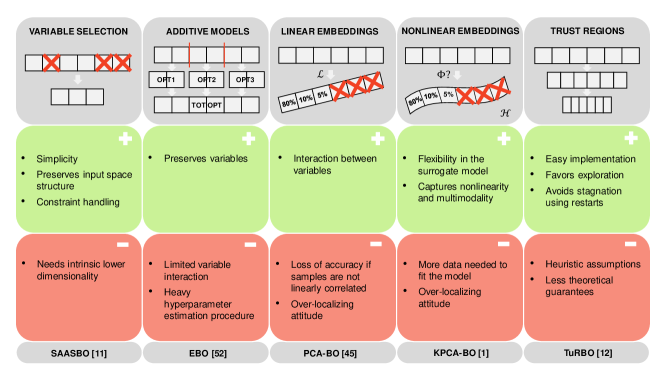
Figure 1. Illustration of the five different categories of BO-based algorithms for high-dimensional problems. The advantages and disadvantages of each category are listed, along with the algorithm chosen for our comparison.

Each of the five HDBO classes has advantages and disadvantages, and the same applies to the algorithms that belong to them. Figure 1 summarizes the idea behind each approach and its pros and cons. To date, there is no consensus on which method is preferable under which circumstances (problem landscape, evaluation budget, and dimensionality).

3. Experimental Setup

We compare the algorithms on the 24 noiseless functions of COCO’s BBOB suite (Hansen et al., 2021). We access these functions via IOHprofiler (Doerr et al., 2018). After initial exploration of the data with IOHanalyzer, we use Python post-processing libraries to generate the plots visualizing our results in this paper.

The BBOB functions on which we base our evaluation are divided into five groups: separable functions (f1-f5), functions with low or moderate conditioning (f6-f9), functions with high conditioning and unimodal structure (f10-f14), multimodal functions with appropriate global structure (f15-f19), and multimodal functions with weak global structure (f20-f24) (Hansen et al., 2009). In our experience, the problems belonging to the last two groups are most representative of real-world problems, as they have a more complex landscape characterized by high nonlinearity and roughness, with multiple peaks or valleys. For each function, we consider dimensions 10, 20, 40, and 60. For SAASBO we did not run complete experiments for dimensions 20, 40 and 60 due to time and memory constraints. In this case, we preferred to perform experiments on functions belonging to the last two groups (f15-f24). Thus, we conducted 10 independent runs of each algorithm for three different instances (instance ID 0-2) of the 24 BBOB functions, with the only exception of SAASBO. For this algorithm, we have:

• data for functions f1-f24 at dimension 10,

• data for functions f15-f24 at dimension 20,

• no data for dimension 60 (infeasible amount of computational time and memory required).

We compare the HDBO algorithms with a vanilla BO from  (Pedregosa et al., 2011) and a default CMA-ES (Hansen et al., 2019).

For each run, the total evaluation budget is set to $10D+50$ function evaluations. For BO-based algorithms, the initial DoE size is set to $D$. By default for the BBOB suite, the domain is set to $[-5,5]^{D}$. For each algorithm described in Section 2.1, we use default settings for their hyperparameters. The implementation of vanilla BO is taken from the Python module scikit-learn, choosing Expected Improvement (EI) as the acquisition function and a noise level equal to $0.01$. The implementation for CMA-ES (Hansen et al., 2019) is the one in the pycma package, available from the GitHub repository pycma. The code for SAASBO is taken from the GitHub repository saasbo. The EBO code is taken from the GitHub repository Ensemble-Bayesian-Optimization, but we redefine the acquisition function as the EI, because the default implementation uses a global minimum value that is assumed to be known, while we assume that it works in a complete black-box scenario. In the experiments, two different implementations of the EBO algorithm are utilized: EBO and EBO_B. They differ for the value of the hyperparameter $B$ that represents the number of query points selected at each iteration. We use $B=1$ and $B=10$, respectively. To use the same total budget, EBO_B runs for budget/10 iterations. The code for PCA-BO and KPCA-BO is taken from the GitHub repository Bayesian-Optimization. The TuRBO code is taken from the GitHub repository TuRBO. In our experiments, two different implementations of TuRBO are compared: TuRBO1 and TuRBOm. They differ in the number of trust regions used by the algorithm: $tr=1$ and $tr=\lfloor D/5\rfloor$, respectively, where $tr$ denotes the number of trust regions and $\lfloor\cdot\rfloor$ denotes the floor function. For more details on the individual algorithms and the values used for the hyperparameters, please refer to the appendix. The code to run the experiments is a modular framework compatible with IOHprofiler. It is available on GitHub in the repository IOH-HDBO-Comparison. We used Python post-processing libraries to present our results and the statistical Wilcoxon signed-rank test to confirm what can be seen through direct inspection of the plots.

4. Results

4.1. Dimension D = 10

4.1.1. Solution Quality

Figure 2. The best-so-far target gap for dimension 10.

Figure 2 compares the convergence behavior of all algorithms on all BBOB functions from f1 to f24 in dimension 10. For a small evaluation budget, vanilla BO always performs better than CMA-ES, as we can see in particular on f2-f4, f12, and f19. However, at the end of the budget, CMA-ES outperforms or is comparable to vanilla BO in many cases. Overall, we see a good performance of vanilla BO, which is due to the still low dimensionality. BO is always among the best or at least comparable to the other algorithms, with a few exceptions. It reaches a particularly good performance on f5, f6, f22, and f24. In Figure 2, algorithm performance is not stable across functions. However, SAASBO and TuRBO tend to predominate. Specifically, TuRBO finds excellent loss values on f2, f3, f13, f14, f16, f18, f20, and f22 (here together with SAASBO). Stagnation at a very low budget is a common behavior of PCA-BO, KPCA-BO, and both EBO and EBO_B (f1, f5, f6, and f20-f22). Finally, if we focus on f5 (linear slope), we can observe the extremely good performance of BO and SAASBO, which are able to immediately find the global optimum due to the unimodal and monotonic landscape of this function (this observation holds for all tested dimensions).

4.1.2. CPU time

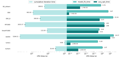
Figure 3. CPU time in seconds (logarithmic scale) for the entire run (left) and model fitting and acquisition function optimization (right) in dimension 40. Values for the total CPU time are averaged across all 24 BBOB functions. Model fitting time and acquisition function optimization time are first averaged over all iterations of one run, and then across the 24 BBOB functions. The black line in each bar represents the bootstrap confidence interval.

In Figure 3, we compare the CPU time in seconds (logarithmic scale) to complete the entire run and the CPU time taken by the different algorithms to fit the GPR model and optimize the acquisition function. We also show the bootstrap confidence interval by the black line in each bar (DiCiccio and Efron, 1996). We can clearly see that SAASBO is the most expensive strategy in terms of total CPU time with an average of 5 284.51 seconds. The two versions of TuRBO are the fastest. They are followed by EBO_B, PCA-BO, and vanilla BO. According to the right side of the plot in Figure 3, SAASBO is also the one that takes more time to complete both steps, fitting the model and optimizing the acquisition function. For almost all algorithms, the CPU time for optimizing the acquisition function is shorter than that for building the model. For PCA-BO and KPCA-BO, they are comparable. From the analyses of convergence and CPU time at 10D, TuRBO1 and TuRBOm seem to perform best.

4.2. Dimension D = 20

4.2.1. Solution Quality

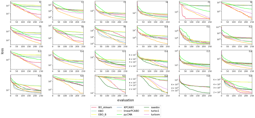
Figure 4. The best-so-far target gap for dimension 20.

Figure 4 compares the convergence behavior of the algorithms on the 20-dimensional problems. We recall that for SAASBO we only have results for f15-f24, due to its high running time. The overall behavior of the BO algorithms and CMA-ES is very similar to that observed for dimension 10. In particular, we see that vanilla BO always outperforms CMA-ES for small budgets, but CMA-ES catches up for a larger budget of 100 evaluations in many cases (f2-f4, f9, f11, f12, and f14). At a high level, vanilla BO is either better or at least comparable to CMA-ES for the entire budget for all multimodal BBOB functions (f15-f24). We can attribute this to the CMA-ES overlocalizing search attitude. It is also interesting to note that at dimension 20, vanilla BO still shows very good performance for some of the functions compared to the BO variants that are specifically designed for high-dimensional problems. In particular, it has one of the best average performances among all algorithms on function f8 and the best one on functions f5 and f24. SAASBO and TuRBO1 are the two HDBO variants whose average performance is best among all tested algorithms for the largest number of functions. Their competitive advantage over the other algorithms is clearly visible in the convergence plots in Figure 4, in particular, true for f1, f2, f13, and f20-f23.

4.2.2. CPU time

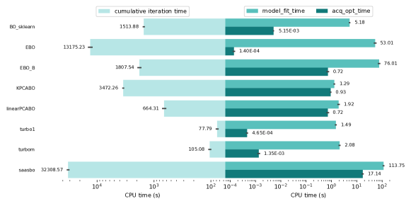
Figure 5. CPU time in seconds (logarithmic scale) for the entire run (left) and model fitting and acquisition function optimization (right) in dimension 40. Values for the total CPU time are averaged across all 24 BBOB functions. Model fitting time and acquisition function optimization time are first averaged over all iterations of one run, and then across the 24 BBOB functions. The black line in each bar represents the bootstrap confidence interval.

Figure 5 compares the CPU times for the entire run, for the modeling phase, and for the optimization of the acquisition function for each algorithm tested. As the figure shows, the time increases significantly compared to dimension 10. Again, the fastest methods are the two versions of TuRBO, while SAASBO reaches a prohibitive total CPU time. Moreover, the CPU time for optimizing the acquisition function is generally much shorter than that for building the model.

Considering the two different analyses, the experimental results suggest that the best algorithm in dimension 20 is TuRBO1. It seems particularly well suited for f20-f22, which belong to the category of multimodal functions with weak global structure.

4.3. Dimension D = 40

4.3.1. Solution Quality

Figure 6 shows the convergence plots for dimension 40.

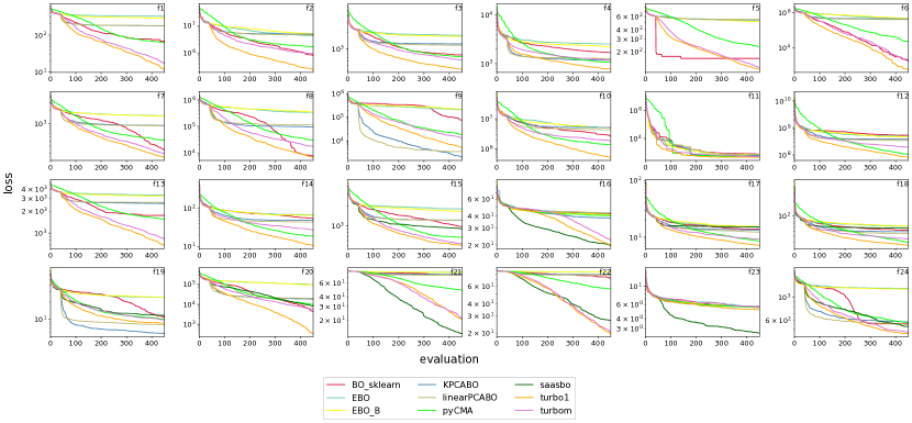
Figure 6. The best-so-far target gap for dimension 40.

We start seeing that vanilla BO scales badly with increasing dimensionality. For a low budget, of $5D$, i.e., 200 function evaluations, BO is never competitive, with the only exception of f5. The best algorithms remain SAASBO and TuRBO1 for most functions. However, we can also notice that on f9 and f19, the KPCA-BO algorithm, followed by PCA-BO, performs significantly better than all the other methods for the entire evaluation budget. We attribute this to the very good global structure of the function landscapes. In this case, PCA-BO and KPCA-BO are more capable of properly capturing the isocontour of the objective function and it is more likely that basins of attraction are detected.

4.3.2. CPU time

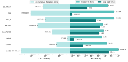
Figure 7. CPU time in seconds (logarithmic scale) for the entire run (left) and model fitting and acquisition function optimization (right) in dimension 40. Values for the total CPU time are averaged across all 24 BBOB functions. Model fitting time and acquisition function optimization time are first averaged over all iterations of one run, and then across the 24 BBOB functions. The black line in each bar represents the bootstrap confidence interval.

In Figure 7, the three different CPU times of the algorithms confirm a prohibitive CPU time for SAASBO, while the computational efficiency of TuRBO1 compared to the other algorithms is even more evident than it was for lower dimension. TuRBO is efficient in terms of CPU time because the Thompson Sampling approach substitutes the sub-optimization of a traditional acquisition function. Finally, it is interesting to observe that also EBO has a low CPU time for optimizing the acquisition function, but this advantage cannot outweigh its poor convergence performance.

Considering the two different analyses, for dimension 40 we can firmly support the predominance of TuRBO1 over the other algorithms.

4.4. Dimension D = 60

4.4.1. Solution Quality

Figure 8. Best-so-far target gap for dimension 60.

Figure 8 compares the convergence behavior of the algorithms for the 60-dimensional BBOB problems. Due to computational constraints, SAASBO is completely missing, as explained in Section 3. The figure demonstrates how BO suffers from a lower convergence rate at high dimensionality. In all cases except for f5, better convergence capabilities of CMA-ES are evident. BO suffers from premature stagnation, which is due to its higher computational complexity in dimension 60. We can observe the same behavior for some HDBO methods, such as EBO and, in some cases, linear and kernel PCA-BO. The performance of BO decreases even on f24, where it was the best solver at lower dimensions. Both versions of TuRBO show very good performance for f1, f13, f21, and f22, and there is a statistically significant difference between them and the other algorithms, which we confirmed by running a Wilcoxon signed-rank test. Moreover, it is worth noting that TuRBO is the only algorithm that continues to improve as the number of evaluations increases, while the other algorithms stagnate easily. Nonetheless, we can observe interesting performance of PCA-BO and KPCA-BO in some cases. They find excellent loss values on f9, f11, f18-f20, and f24, where they either rank first or show initial speedups that make them good candidates for high-dimension/low-budget optimization problems. EBO and EBO_B perform poorly. We attribute this to the choice of their hyperparameters as the default ones, which might not be ideal for the function landscapes addressed in this study.

4.4.2. CPU time

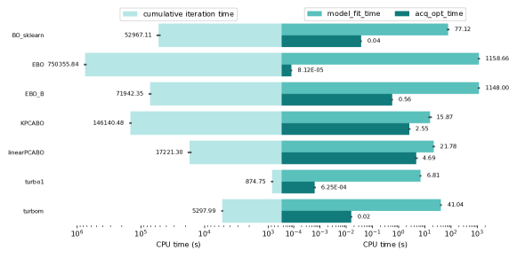
Figure 9. CPU time in seconds (logarithmic scale) for the entire run (left) and model fitting and acquisition function optimization (right) in dimension 40. Values for the total CPU time are averaged across all 24 BBOB functions. Model fitting time and acquisition function optimization time are first averaged over all iterations of one run, and then across the 24 BBOB functions. The black line in each bar represents the bootstrap confidence interval.

In Figure 9, on the left, we can see that EBO and KPCA-BO are the algorithms that require the highest CPU time for the run. Again, TuRBO1 is significantly better than the other algorithms and the difference in performance between TuRBO1 and TuRBOm becomes clearer, which suggests the use of just one trust region for high-dimensional problems. On the right-hand side, Figure 9 confirms that the CPU time for optimizing the acquisition function is generally much shorter than the time required for fitting the model, with almost comparable values for linear and kernel PCA-BO, given that both steps are performed in a mapped space with reduced dimensionality. Finally, we note that the time taken to optimize the acquisition function varies widely between algorithms. This shows that great efforts have been made to improve the efficiency of the infill criterion, which is a main differentiating trait between the algorithms studied.

5. Further Discussion

For an in-depth comparison, we also present in Figure 10 violin plots that compare the performance of three candidate algorithms for each BBOB function for dimension 40: vanilla BO, CMA-ES, and the best among the HDBO algorithms for a specific function at the end of the budget (see the appendix for similar violin plots for dimensions 10, 20, and 60). While BO is usually outperformed by CMA-ES at the end of the evaluation budget, the best among the HDBO algorithms always performs better than CMA-ES.

In general, we can see that TuRBO1 performs the best in dimension 40. However, there are some exceptions: KPCA-BO on f9 and f19, and SAASBO on f21 and f23.

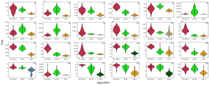
Figure 10. The violin plots show, for dimension 40 and budget 450 (final budget), the distribution of the best-so-far loss values for all functions, obtained by vanilla BO, CMA-ES, and the best among the HDBO algorithms. The plots include a marker for the median of the data and a box indicating the interquartile range.

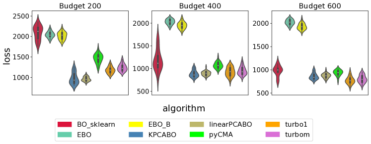
Figure 11. Violin plots showing loss values at three different budgets (200, 400, and 600 function evaluations) for function 24.

Figure 11 shows the convergence evolution of the algorithms compared on f24 at dimension 60, by freezing it at three different budgets: 200, 400, and 600 evaluations. The figure gives an idea of the ranking of the algorithms in different phases of the optimization runs and clearly shows in which context one of the algorithms is preferable to the others. For a limited budget (Figure 11, budget 200), PCA-BO and KPCA-BO find the lowest loss values. We attribute this to their better ability to find good solutions in a lower-dimensional manifold of the original search space. However, this often drives the search towards local optima. Already at budget 400 (Figure 11, budget 400), PCA-BO and KPCA-BO become comparable to the other HDBO algorithms and they are significantly outperformed at the end of the run (Figure  11, budget 600). At this point, TuRBO1 and TuRBOm represent the best choice. In fact, TuRBO seems to offer a better balance between exploration and exploitation of the domain by using dynamic trust regions and multiple restarts. Based on a Wilcoxon signed-rank test, these results are statistically significant. Given these observations, we believe that it would be interesting to explore the possibility of combining the concepts behind PCA-BO and TuRBO, by building local low-dimensional embeddings. In this way, one can benefit from both the flexibility of the trust regions and the lower complexity of the manifolds with reduced dimension. We leave this to our future research.

6. Conclusion and Future Perspectives

In this work, we have conducted an experimental study comparing the performance of vanilla BO, CMA-ES, and five BO-based algorithms designed to improve BO performance in high-dimensional search spaces. For our tests, we selected one representative for each of the main categories of algorithms for high-dimensional BO: SAASBO for variable selection, EBO for additive models, PCA-BO and KPCA-BO for linear and nonlinear embeddings respectively, and TuRBO for trust regions. We compared the algorithms on the 24 functions from the BBOB benchmark suite from the COCO benchmarking environment, by running 10 repetitions of each algorithm on 3 different instances of each function, with some exceptions due to time and memory constraints.

Our results confirm a good performance of BO at low dimension (10D), which gradually deteriorates as the dimensionality of the problem increases. Here, CMA-ES performs better, especially for larger budgets. However, the average observed performance of CMA-ES is worse than that of the HDBO algorithms. Although we observe different performance for different function landscapes and budget utilization phases, TuRBO seems to be the most promising algorithm, both in terms of convergence trend and CPU time. However, PCA-BO and KPCA-BO also show potential for small evaluation budgets, with very fast convergence towards a near-optimal solution.

Therefore, further work is planned to develop a hybrid algorithm that combines PCA-BO and TuRBO. This algorithm could avoid the stagnation of PCA-BO by using restarts and trust regions and still benefit from a linear low-dimensional embedding, resulting in a very competitive algorithm for optimizing expensive black-box functions at high dimensionality. Moreover, we aim at creating a modular framework that allows for choosing a convenient strategy for each optimization phase of BO, such as model fitting and acquisition function optimization, to obtain combinations of the selected algorithms and improvement over the current state of the art. We also found that the poor performance of some algorithms, especially EBO, could be caused by poor initialization of their hyperparameters. Hence, we plan to investigate how they could benefit from hyperparameter optimization and repeat our comparative analysis.

Appendix

Appendix A Algorithms

Here we provide the reader with a more detailed description of the algorithms that were compared in our study and the chosen hyperparameter settings.

A.1. Covariance Matrix Adaptation Evolution Strategy (CMA-ES)

Covariance Matrix Adaptation Evolution Strategy (CMA-ES)) (Hansen, 2006; Hansen and Kern, 2004; Hansen et al., 2003) belongs to the family of evolutionary algorithms (Vikhar, 2016; Simionescu et al., 2006) and is considered to be the state-of-the-art in this category, being the most commonly used for continuous optimization in many research laboratories and industrial environments. CMA-ES is mostly used to solve difficult nonlinear nonconvex black-box optimization problems, unconstrained or constrained, in continuous domains. It efficiently addresses search spaces of dimension between three and one hundred. CMA-ES is based on an idea similar to the Quasi-Newton method (Nocedal and Wright, 1999), that is, it is a second-order estimator that estimates a positive definite matrix, the covariance matrix, in an iterative way. Unlike the Quasi-Newton method, CMA-ES does not use or approximate gradients and does not even assume their existence. For this reason, it can be used for non-smooth and even non-continuous problems, as well as for multimodal and/or noisy problems. Furthermore, CMA-ES does not require expensive hyperparameter tuning, since the choice of hyperparameters is not left to the user (apart from population size). Also, restarts with increasing population size improve the global search performance. The only hyperparameters that the user needs to set for the application of CMA-ES are an initial parent design, an initial step-size, and a termination criterion.

In this study, the initial solution was taken as a random sample array in the design space and the initial step-size in each coordinate is equal to 1. We considered a default population size of $4+3\log D$, where $\log D$ is the natural logarithm of the dimension of the design domain.

A.2. Sparse Axis-Aligned Subspaces BO (SAASBO)

One of the most difficult problems with high-dimensional BO is defining an appropriate class of surrogate models. On the one hand, a class of models that is too flexible may lead to overfitting. On the other hand, a class that is too rigid would not be able to capture the important properties of the objective function landscape.

Sparse Axis Aligned Subspace Bayesian Optimization (SAASBO) (Eriksson and Jankowiak, 2021) introduces a new surrogate model for high-dimensional BO based on the assumption that the coordinates of $x\text{ in }S$ have a relevance hierarchy. According to (Eriksson and Jankowiak, 2021) this approach has several key advantages. First, it preserves the structure of the input space and therefore it can exploit it. Second, it is adaptive and shows low sensitivity to its hyperparameters. Third, it can naturally accommodate both input and output constraints, unlike methods based on random projections for which input constraints are particularly challenging. In SAASBO, the usual Gaussian process is used, but with the help of some new components.

The innovations are:

• sparsity-inducing SAAS function prior;

• combination of the surrogate model with the No-Turn-U-Sampler (NUTS), an adaptive form of Hamiltonian Monte Carlo (HMC) sampling that the algorithm must perform to do inference on that model. It allows the surrogate model to quickly identify the most important low-dimensional subspace, resulting in a sample-efficient BO.

In our experiments we set the following values for the main hyperparameters:

• $\alpha=0.1$, a positive float that controls the level of shrinkage/sparsity of the GP model. Smaller alpha for more sparsity, and so most dimensions “turned off”;

• num_warmup = 256, the number of warmup samples to use in the NUTS. During warmup, the NUTS algorithm adjusts the HMC algorithm parameters metric and step-size in order to sample efficiently. After the warmup, the fixed metric and step-size are used to produce a set of draws;

• num_samples = 256, the number of post-warmup samples to use in HMC inference;

• thinning = 32, a positive integer that controls the fraction of posterior hyperparameter samples that are used to compute the expected improvement;

• kernel = rbf. By default, SAASBO uses radial basis function kernels in the GP model definition.

A.3. Ensemble BO (EBO)

When dealing with high-dimensional problems, the inefficiency of BO occurs not only in the creation of the surrogate model but also in the optimization of the acquisition function, which is sometimes very expensive to evaluate. Moreover, reliable search and estimation for complex functions in very high-dimensional spaces may require a large number of observations. Ensemble Bayesian Optimization (EBO)  (Wang et al., 2018) attempts to answer precisely these three challenges:

1. large-scale observations,

2. high-dimensional input spaces,

3. selection of batches of query points that balance quality and diversity.

To achieve this, EBO uses an ensemble of additive Gaussian process models, each of which has a randomized strategy for division and conquest. The two main ideas implemented at several levels are the use of efficient partitioning-based function approximators that take into account both data and features to simplify and speed up the search, and the expressive power of these approximators through the use of ensembles and a stochastic approach. In fact, to solve the three challenges, the authors propose to improve the GP models by using a hierarchical additive approach based on tile coding, also known as random binning or Mondrian Forest features. Then, thanks to a Gibbs sampling, the posterior distribution is learned over the kernel width and the additive structure to prevent overfitting. The third challenge is to improve the sampler which depends on the likelihood of the observations. This is accelerated by an efficient randomized block approximator of the Gram matrix based on a Mondrian process.

We set the following values for the main hyperparameters:

• z = sample_z(D). This parameter controls the additive decomposition of the input feature space. It is an array of dimension D and it can assume only discrete values. Here it is selected randomly through the method sample_z;

• k = array([10] * D), the number of cuts in each dimension. It is an array of dimension D and it can assume only discrete values;

• $\alpha=1$, hyperparameter of the Gibbs sampling subroutine;

• $\beta=\text{array}([5.,2.])$, hyperparameter of the Gibbs sampling subroutine;

• opt_n = 1000 points randomly sampled to initiate the continuous optimization of the acquisition function;

• gibbs_iter = 10 number of iterations for the Gibbs sampling subroutine;

• nlayers = 100, number of the layers of tiles;

• gp_sigma = 0.1, noise standard deviation;

• n_top = 10, how many points to look ahead when selecting the new infill point.

A.4. Linear PCA-assisted Bayesian Optimization (PCA-BO)

Another method for scaling BO for high-dimensional data is based on the use of the well-known technique of Principal Component Analysis (PCA) to generate a new BO algorithm called PCA-assisted Bayesian optimization (PCA-BO) (Raponi et al., 2020). Thanks to PCA, the algorithm learns a linear transformation based on the points evaluated so far and selects the dimensions in the transformed space considering the variability of these points. Both the fitting of the GPR model and the optimization of the acquisition function are carried out in the space with reduced dimensionality. The primary benefits are the reduction of CPU time for high-dimensional problems and the ability to maintain a good convergence rate for problems with an adequate global structure.

PCA-BO starts with a DoE and adaptively learns a linear map, updated at each iteration, to reduce the dimensionality through a weighted PCA procedure. Weights are used to account for objective values.

The main steps of the PCA-BO algorithm can be summarized as follows:

1. Generate an initial DoE in the original space composed of a set of evenly distributed points;

2. Design a weighted scheme to take into account the information from the objective function into the DoE points: smaller weights are assigned to the points with worse function values.

3. Apply the PCA technique to create a linear map from the original search space to a lower-dimensional space, using the weighted DoE points;

4. Train a GPR model and maximize an infill criterion to find the new infill point, both in the lower-dimensional space;

5. Map back the infill point to the original space and evaluate its objective function value;

6. Append the new infill point and its objective value to the data set and then proceed to Step 2 for a new iteration.

We set the following values for the main hyperparameters:

• n_point = 1, the number of infill points selected during the optimization of the acquisition function;

• n_components = 0.90, the amount of variance that needs to be explained by the principal components kept after dimensionality reduction by PCA;

• acquisition_optimization = BFGS, optimizer used to maximize the acquisition function.

A.5. Kernel PCA-assisted BO (KPCA-BO)

The kernel PCA-assisted algorithm BO (KPCA-BO) (Antonov et al., 2022) is an extended version of PCA-BO, which uses kernel methods to first map points to a reproducing kernel Hilbert space (RKHS) (Berlinet and Thomas-Agnan, 2011) using an implicit nonlinear feature mapping. Then, PCA is used in the RKHS to learn a linear transformation from all evaluated points during the run and select dimensions in the transformed space according to the variability of the evaluated points. The main advantage of KPCA-BO over PCA-BO is the nonlinearity of the submanifold in the search space, which makes it more likely that multiple basins of attraction will be discovered simultaneously. Besides learning a forward map from the original space to a lower-dimensional submanifold, it constructs a backward map that converts an infill point determined in the reduced space to the original space, so that it can be evaluated. In this way, the two most extensive procedures of BO, training the GP model and optimizing the acquisition function, are performed in a low-dimensional space, reducing CPU time.

We set the following values for the main hyperparameters:

• n_point = 1, the number of infill points selected during the optimization of the acquisition function;

• max_information_loss=0.1, the decimal value of the maximum information of variability data points that can be lost during the PCA procedure in the Hilbert space;

• kernel_fit_strategy = KernelFitStrategy.AUTO. The AUTO setting uses an RBF kernel.

A.6. Trust Region BO (TuRBO)

There are two key issues that often lead to poor performance of classical BO in high-dimensional settings: the homogeneity of global probabilistic models and overemphasized exploration due to global coverage. To overcome these problems, the global perspective can be discarded, and a local approach can be used.Trust regions BO (TuRBO) (Eriksson et al., 2019) is a technique for global optimization that uses a collection of simultaneous local optimization runs with independent probabilistic models. To combine all the local parts and return to a global vision, an implicit multi-armed bandit strategy is used at each iteration to distribute the samples across different local domains and hence decide which local optimization runs are preferred. In each global iteration, which means considering all the trust regions, the algorithm selects a batch of $q$ candidates drawn from the union of all the trust regions, and updates all the local models for which candidates were drawn. A Thompson sampling (Hernández-Lobato et al., 2016) is used to select infill points within a single trust region and in all trust regions simultaneously.

The main advantages of this approach are that (1) each local surrogate model is robust to noisy observations and uncertainty estimates, (2) the local surrogates allow heterogeneous modeling of the objective function and do not suffer from overexploitation, and (3) it provides local search trajectories that are able to quickly discover excellent target values.

We set the hyperparameters as follows:

• batch_size = 5, number of infill points found in each iteration,

• max_cholesky_size = 2000, after how many iterations the algorithm switches from Cholesky to Lanczos to train the GP;

• n_training_steps = 50, number of steps of ADAM to learn the hyperparameters of the GP;

• n_cand = min(100 * D, 5000), number of vectors of dimension D generated by a Sobolev sequence where to evaluate the batch_size GP samples;

• failtol = ceil(max([4.0/ batch_size, D/batch_size])) for TuRBO1 and failtol = max(5, D) for TuRBOm, where ceil of the scalar $x$ is the smallest integer $i$ such that $i\leq x$ and it is the threshold for failures after which trust regions halves;

• succtol = 3, the threshold for successes after which trust regions doubles;

• length_min = $0.5^{7}$, the minimum threshold for the base side length of the trust regions before restart;

• length_max = 1.6, the maximum threshold for the base side length of the trust regions;

• length_init = 0.8, value to initialize the base side length of the trust regions.

Appendix B Extensive CPU time analysis

Figures 12, 13, 14, and 15 present additional bar plots for the CPU time required to fit the model, optimize the acquisition function, and perform the complete run, for each method and on each BBOB function.

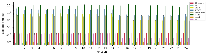
(a)

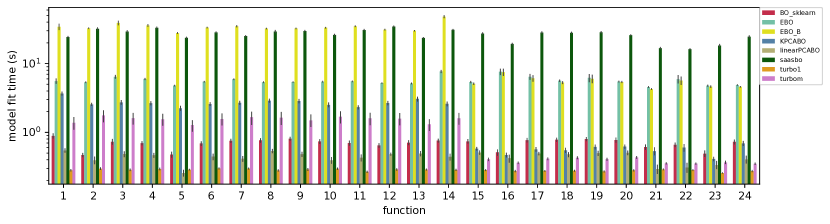
(b)

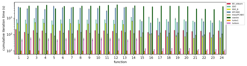
(c)

Figure 12. CPU time bar plots for 10D, function by function.

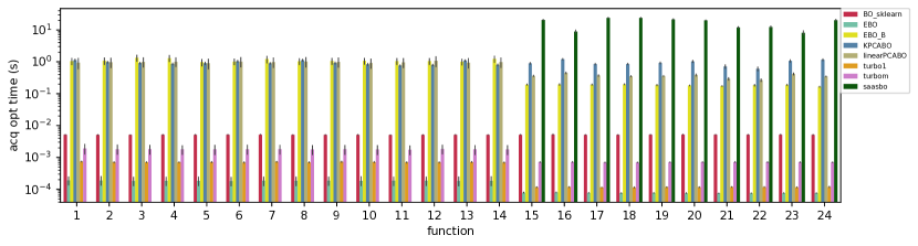
(a)

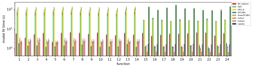
(b)

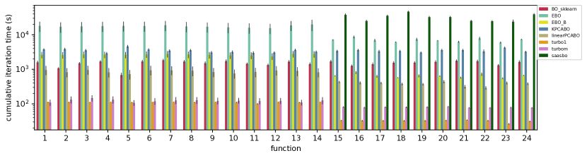
(c)

Figure 13. CPU time bar plots for 20D, function by function.

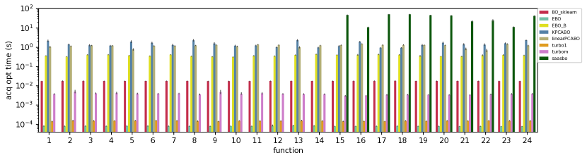
(a)

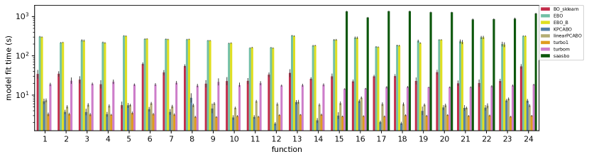
(b)

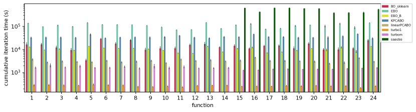
(c)

Figure 14. CPU time bar plots for 40D, function by function.

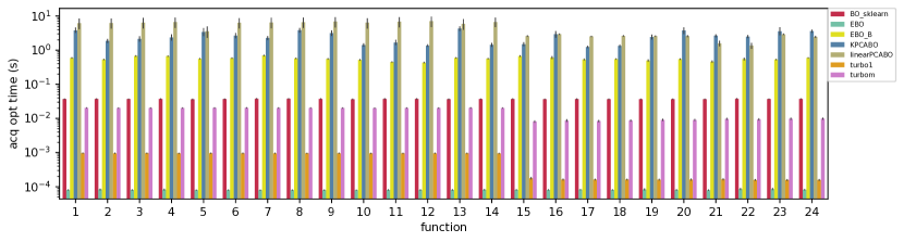
(a)

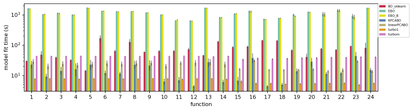
(b)

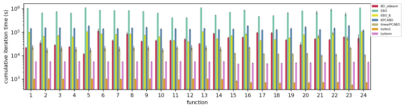
(c)

Figure 15. CPU time bar plots for 60D, function by function.

Appendix C Violin Plots

Figures 16, 17, and 18 provide a comparison through violin plots for the performance of standard BO, CMA-ES, and the best among the HDBO algorithms for each setting (combination of function and dimension) at the end of the budget. Here we show results for dimensions 10, 20, and 60, while dimension 40 was already discussed in Section 5.

Figure 16. The violin plots show, for dimension 10 and budget 150 (final budget), the distribution of the best-so-far function values for all functions, obtained by vanilla BO, CMA-ES, and the best among the HDBO algorithms. The plots include a marker for the median of the data and a box indicating the interquartile range.

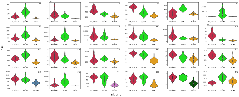
Figure 17. The violin plots show, for dimension 20 and budget 250 (final budget), the distribution of the best-so-far function values for all functions, obtained by vanilla BO, CMA-ES, and the best among the HDBO algorithms. The plots include a marker for the median of the data and a box indicating the interquartile range.

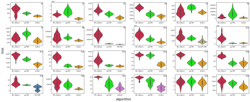
Figure 18. The violin plots show, for dimension 60 and budget 650 (final budget), the distribution of the best-so-far function values for all functions, obtained by vanilla BO, CMA-ES, and the best among the HDBO algorithms. The plots include a marker for the median of the data and a box indicating the interquartile range.