Variance-reduced Clipping for Non-convex Optimization

Abstract

Gradient clipping is a standard training technique used in deep learning applications such as large-scale language modeling to mitigate exploding gradients. Recent experimental studies have demonstrated a fairly special behavior in the smoothness of the training objective along its trajectory when trained with gradient clipping. That is, the smoothness grows with the gradient norm. This is in clear contrast to the well-established assumption in folklore non-convex optimization, a.k.a. $L$–smoothness, where the smoothness is assumed to be bounded by a constant $L$ globally. The recently introduced $(L_{0},L_{1})$–smoothness is a more relaxed notion that captures such behavior in non-convex optimization. In particular, it has been shown that under this relaxed smoothness assumption, Sgd with clipping requires ${\mathcal{O}}(\epsilon^{-4})$ stochastic gradient computations to find an $\epsilon$–stationary solution. In this paper, we employ a variance reduction technique, namely Spider, and demonstrate that for a carefully designed learning rate, this complexity is improved to ${\mathcal{O}}(\epsilon^{-3})$ which is order-optimal. Our designed learning rate comprises the clipping technique to mitigate the growing smoothness. Moreover, when the objective function is the average of $n$ components, we improve the existing ${\mathcal{O}}(n\epsilon^{-2})$ bound on the stochastic gradient complexity to ${\mathcal{O}}(\sqrt{n}\epsilon^{-2}+n)$, which is order-optimal as well. In addition to being theoretically optimal, Spider with our designed parameters demonstrates comparable empirical performance against variance-reduced methods such as Svrg and Sarah in several vision tasks.

1 Introduction

We study the problem of minimizing a non-convex function $F\mathrel{\mathop{\mathchar 58\relax}}{\mathbb{R}}^{d}\to{\mathbb{R}}$ which is expressed as the expectation of a stochastic function, i.e.,

$$\operatorname*{minimize}_{{\mathbf{x}}\in{\mathbb{R}}^{d}}\,\,F({\mathbf{x}})=\mathbb{E}_{\xi}[f({\mathbf{x}};\xi)],$$ (1)

where the random variable $\xi$ is realized according to a distribution ${\mathcal{D}}$. Typically, the distribution ${\mathcal{D}}$ is unknown in this stochastic setting, and rather, a number of realized samples are available. In this setting, known as finite-sum, the objective $F$ can be expressed as the average of $n$ component functions $f_{1},\cdots,f_{n}$, that is,

$$\operatorname*{minimize}_{{\mathbf{x}}\in{\mathbb{R}}^{d}}\,\,F({\mathbf{x}})=\frac{1}{n}\sum_{i=1}^{n}f_{i}({\mathbf{x}}).$$ (2)

This formulation captures the standard training framework in many machine learning and deep learning applications where the model parameters are trained by minimizing the average loss induced by a large number of labeled data samples (also known as empirical risk minimization).

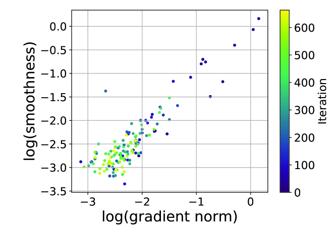
(a) AWD-LSTM training using gradient clipping

(b) Transformers training using Adam

Figure 1: Smoothness grows with gradient norm along the training trajectory for (a) AWD-LSTM on PTB dataset trained with clipped Sgd (Figure taken from Zhang et al. (2019)), and (b) transformers on WMT 2014 translation dataset trained with Adam (Figure taken from Wang et al. (2022)).

Gradient-based algorithms such as stochastic gradient descent (Sgd) have been widely used in training deep learning models due to their simplicity. However, adaptive gradient methods demonstrate superior performance over Sgd in particular applications such as natural language processing (NLP). In such methods, gradient clipping has been a standard practice in training language models to mitigate the exploding gradient problem. Although such superior performance of gradient clipping has not been well justified theoretically, (Zhang et al., 2019) brings about some rationales to better understand the probable underpinning phenomenon. To bridge the theory-practice gap in this particular application, (Zhang et al., 2019) first demonstrates an interesting characteristic of the optimization landscape of large-scale language models such as LSTM trained with gradient clipping. As illustrated in Figure 1, the smoothness of the objective grows with the gradient norm along the training trajectory. This defies a well-established belief in smooth non-convex optimization where the smoothness is assumed to be bounded by a constant over the input space, that is, $\|\nabla^{2}F({\mathbf{x}})\|\leq L$. Inspired by the experimental evidence, (Zhang et al., 2019) introduces the more relaxed smoothness notion named $(L_{0},L_{1})$-smoothness, where the smoothness grows linearly with the gradient norm, that is, $\|\nabla^{2}F({\mathbf{x}})\|\leq L_{0}+L_{1}\|\nabla F({\mathbf{x}})\|$ for positive constants $L_{0},L_{1}$. This class of nonconvex functions includes many instances that do not have global Lipschitz gradients, such as the so-called exponential family. In particular, all polynomials of degree at least $3$, are $(L_{0},L_{1})$–smooth while there exists no constant bounding the smoothness globally (Zhang et al., 2019).

The standard performance measure of non-convex optimization algorithms is their required gradient computation to find approximate first-order stationary solutions. More precisely, the goal of any non-convex optimization algorithm is to find a solution ${\mathbf{x}}$ such that

$$\|\nabla F({\mathbf{x}})\|\leq\epsilon,$$ (3)

for a given target accuracy $\epsilon$. The total number of gradient computations to find such a stationary point is defined as the first-order oracle or gradient complexity for the corresponding algorithm. Employing gradient clipping, Zhang et al. (2019) show that clipped Sgd is able to find an $\epsilon$–stationary solution of any $(L_{0},L_{1})$–smooth non-convex objective with gradient complexity at most ${\mathcal{O}}(\epsilon^{-4})$. In this paper, we aim to answer the following question:

We answer this question in the affirmative. In particular, we employ variance reduction techniques and show that under regular conditions, the gradient complexity of finding an $\epsilon$–stationary point can be improved to ${\mathcal{O}}(\epsilon^{-3})$ which is order-optimal.

Variance reduction has been a promising approach in speeding up non-convex optimization algorithms for $L$–smooth objectives. Most relevant to our work is Spider algorithm proposed in (Fang et al., 2018). The core idea of Spider is to devise and maintain an accurate estimator of the true gradient along the iterates. Let ${\mathbf{v}}_{k}$ denote the Spider’s estimator for the true gradient $\nabla F({\mathbf{x}}_{k})$ at iterate $k$. The gradient estimator ${\mathbf{v}}_{k}$ is updated in every iteration using a small batch of stochastic gradients and the previous ${\mathbf{v}}_{k-1}$. To reset the undesired effect of stochastic gradients noise, a large batch is used to update ${\mathbf{v}}_{k}$ once in a while. It has been shown that for a proper choice of the stepsize, Spider is able to control the variance of the gradient estimator by $\epsilon^{2}$ for every iteration. Together with the standard Descent Lemma, (Fang et al., 2018) has shown that Spider requires at most ${\mathcal{O}}(\epsilon^{-3})$ stochastic gradient computations to reach an $\epsilon$–stationary point for any (averaged) $L$–smooth objective function. The adaptive stepsize corresponding to this order-optimal rate is picked as ${\mathcal{O}}(\min\{1,\epsilon/\|{\mathbf{v}}_{k}\|\})$.

In this work, we aim to employ the variance reduction idea in Spider to speed up the clipped Sgd algorithm for $(L_{0},L_{1})$–smooth objectives. The first challenge in doing so is that the standard Descent Lemma for $L$–smooth objectives does not hold under the relaxed $(L_{0},L_{1})$–smooth condition. We show that the clipping component in the stepsize, i.e. $\epsilon/\|{\mathbf{v}}_{k}\|$, equips us to establish a descent property under the new smoothness condition.

The second and more critical challenge in utilizing the Spider approach in our setting is to control the variance of the gradient estimator, that is $\mathbb{E}\|{\mathbf{v}}_{k}-\nabla F({\mathbf{x}}_{k})\|^{2}$. As mentioned before, Fang et al. (2018) show that for $L$–smooth objectives, the variance of the gradient estimator remains bounded by $\epsilon^{2}$ along the iterates if the stepsize is picked as ${\mathcal{O}}(\min\{1,\epsilon/\|{\mathbf{v}}_{k}\|\})$. However, this stepsize does not guarantee bounded variance in our $(L_{0},L_{1})$–smooth setting. In particular, we show that rather a smaller stepsize is required to control the variance. That is, for stepsize ${\mathcal{O}}(\min\{1,\epsilon/\|{\mathbf{v}}_{k}\|,\epsilon/\|{\mathbf{v}}_{k}\|^{2}\})$, the variance of the gradient estimator ${\mathbf{v}}_{k}$ is provably controlled and bounded by $\epsilon^{2}$. The additional term $\epsilon/\|{\mathbf{v}}_{k}\|^{2}$ in the stepsize is essential in mitigating the growth of the smoothness which scales with the gradient norm in the relaxed $(L_{0},L_{1})$–smooth setting. We shall refer to Spider in this smoothness setup with this particular stepsize as $(L_{0},L_{1})$–Spider.

Together with the (new) descent lemma, we show that $(L_{0},L_{1})$–Spider with our devised choice of the learning rate described above, finds an $\epsilon$–stationary point of any non-convex and $(L_{0},L_{1})$–smooth function with high probability. More importantly, we demonstrate that the total stochastic gradient computations required to find such a stationary point is at most ${\mathcal{O}}(\epsilon^{-3})$. In our analysis, we relax the more restricted stochastic gradient assumption of almost surely bounded noise in (Zhang et al., 2019) and impose a conventional and fairly generic assumption of bounded noise variance. In addition, we assume that the objective function is averaged $(L_{0},L_{1})$–smooth over its stochastic components. Imposing the stronger averaged smoothness assumption on top of the weaker and typical one is indeed a standard practice in variance-reduced optimization literature. Under such generic assumptions, it has been shown that the $\Omega(\epsilon^{-3})$ rate is indeed a lower bound on the stochastic gradient complexity for (averaged) $L$–smooth objectives (Fang et al., 2018). Clearly, every $L$–smooth function is $(L,0)$–smooth, as well. Therefore, our ${\mathcal{O}}(\epsilon^{-3})$ gradient complexity bound is also tight for the broader class of $(L_{0},L_{1})$–smooth non-convex functions.

We extend our results to the finite-sum setting (2) and show that for our devised pick of the stepsize ${\mathcal{O}}(\min\{1,\epsilon/\|{\mathbf{v}}_{k}\|,\allowbreak\epsilon/\|{\mathbf{v}}_{k}\|^{2}\})$, the variance reduction approach in Spider is able to find an $\epsilon$–stationary point of any non-convex $(L_{0},L_{1})$–smooth function with high probability and at most ${\mathcal{O}}(\sqrt{n}\epsilon^{-2}+n)$ gradient computations. This significantly reduces the existing gradient complexity of clipped Sgd (Zhang et al., 2019), that is ${\mathcal{O}}(n\epsilon^{-2})$. In addition, the derived ${\mathcal{O}}(\sqrt{n}\epsilon^{-2}+n)$ complexity bound is naturally tight in the $(L_{0},L_{1})$–smooth setting, as that is the case under the more restrictive $L$–smoothness condition. Tables 1 and 2 summarise our discussion.

Algorithm	Reference	Stochastic	Finite-sum
ClippedSGD	Zhang et al. (2019)	${\mathcal{O}}(\epsilon^{-4})$	${\mathcal{O}}(n\epsilon^{-2})$
$(L_{0},L_{1})$–Spider	This paper	${\mathcal{O}}(\epsilon^{-3})$	${\mathcal{O}}(\sqrt{n}\epsilon^{-2}+n)$
Lower bound	Arjevani et al. (2022); Fang et al. (2018)	$\Omega(\epsilon^{-3})$	$\Omega(\sqrt{n}\epsilon^{-2})$†

Table 1: Complexity of $(L_{0},L_{1})$–smooth non-convex optimization. ^†This lower bound holds for $n\leq{\mathcal{O}}(\epsilon^{-4})$.

Smoothness	Reference	Stochastic	Finite-sum	Learning rate
$L$–smooth	Fang et al. (2018)	${\mathcal{O}}(\epsilon^{-3})$	${\mathcal{O}}(\sqrt{n}\epsilon^{-2}+n)$	${\mathcal{O}}\Big{(}\min\Big{\{}1,\frac{\epsilon}{\|{\mathbf{v}}_{k}\|}\Big{\}}\Big{)}$
$(L_{0},L_{1})$–smooth	This paper	${\mathcal{O}}(\epsilon^{-3})$	${\mathcal{O}}(\sqrt{n}\epsilon^{-2}+n)$	${\mathcal{O}}\Big{(}\min\Big{\{}1,\frac{\epsilon}{\|{\mathbf{v}}_{k}\|},\frac{\epsilon}{\|{\mathbf{v}}_{k}\|^{2}}\Big{\}}\Big{)}$

Table 2: Learning rates for Spider and $(L_{0},L_{1})$–Spider. All gradient complexities are order-optimal.

Contributions. To summarize the above discussion, we study non-convex optimization under $(L_{0},L_{1})$–smoothness and improve the existing gradient complexities of reaching first-order stationary solutions in both stochastic and finite-sum settings. We employ variance reduction technique Spider, and devise learning rates resulting in order-optimal gradient complexities. Tables 1 compares this paper’s results with the existing and optimal gradient complexities. In Table 2, the learning rates resulting in order-optimal complexities in the folklore $L$–smooth and new $(L_{0},L_{1})$–smoothness settings are compared. Moreover, we implement Spider with our designed learning rates and compare its empirical performance against several benchmarks such as Sgd, Sarah and Svrg tested on different image classification tasks with MNIST, CIFAR10 and CIFAR100 datasets.

Notation. Throughout the paper, we denote by $\|{\mathbf{a}}\|$ the $\ell_{2}$–norm of vector ${\mathbf{a}}$. We also let $\|{\mathbf{A}}\|$ denote the spectral norm of matrix ${\mathbf{A}}$. For non-negative functions $f,g\mathrel{\mathop{\mathchar 58\relax}}{\mathcal{X}}\to[0,\infty)$ defined on the same domain, the standard big O notation $f={\mathcal{O}}(g)$ summarizes the fact that there exists a positive constant $c>0$ such that $f({\mathbf{x}})\leq c\cdot g({\mathbf{x}})$ for all ${\mathbf{x}}\in{\mathcal{X}}$. Moreover, we denote $f=\Omega(g)$ if there exists a positive constant $c>0$ such that $f({\mathbf{x}})\geq c\cdot g({\mathbf{x}})$ for all ${\mathbf{x}}\in{\mathcal{X}}$. Lastly, we use the shorthand notation ${\mathbf{x}}_{i\mathrel{\mathop{\mathchar 58\relax}}j}$ to denote the sequence ${\mathbf{x}}_{i},\cdots,{\mathbf{x}}_{j}$.

Related work.

$(L_{0},L_{1})$–smoothness and gradient clipping. As mentioned before, gradient clipping has been widely used in training deep learning models such as large-scale language models to circumvent the exploding gradient challenge (Merity et al., 2017; Gehring et al., 2017; Peters et al., 2018). The work of Zhang et al. (2019) lays out a theoretical framework to better understand the superior performance of clipped algorithms over the conventional non-adaptive gradient methods. Several follow-up works have studied the introduced $(L_{0},L_{1})$–smoothness notion by (Zhang et al., 2019). (Zhang et al., 2020) utilizes momentum techniques and sharpens the constant dependency of the convergence rate of clipped Sgd previously derived by (Zhang et al., 2019). Under this relaxed smoothness assumption, (Qian et al., 2021) studies the role of clipping in incremental gradient methods. In the deterministic setting with full batch gradient computation, clipped Gd and normalized Gd (NGD) are essentially equivalent up to a constant. (Zhao et al., 2021) provides convergence guarantees for stochastic NGD for $(L_{0},L_{1})$–smooth non-convex functions. The work of Faw et al. (2023) builds on AdaGrad-type methods and relaxes the existing restrictive assumptions on the stochastic gradient noise. Clipping methods may be implemented with scalability (Liu et al., 2022) and privacy considerations (Yang et al., 2022; Xia et al., 2022) as well. Under the same setting, it has been shown that unclipped methods, particularly a generalized SignSGD algorithm, attain the same rates as clipped Sgd (Crawshaw et al., 2022). Interestingly, this smoothness behavior is not restricted to the clipped Sgd optimizer as implemented by Zhang et al. (2019); training language models with Adam manifests such smoothness phenomena as well (Wang et al., 2022). Apart from the optimization literature, $(L_{0},L_{1})$–smoothness has been studied for variational inference problems as well (Sun et al., 2022).

Variance reduction in non-convex optimization. Variance reduction is known to be an effective approach for accelerating both convex and non-convex optimization algorithms. To recap the convergence rate improvement offered by variance reduction techniques in finding stationary points of non-convex functions with global Lipschitz-gradients (i.e. $L$–smooth), recall the folklore rate ${\mathcal{O}}(\min\{n\epsilon^{-2},\epsilon^{-4}\})$ of Sgd/Gd corresponding to finite-sum and stochastic settings (Nesterov, 2003). Stochastic Variance-Reduced Gradient (SVRG) and Stochastically Controlled Stochastic Gradient (SCSG) improved the gradient complexity to $\tilde{{\mathcal{O}}}(\min\{n^{2/3}\epsilon^{-2},\epsilon^{-10/3}\})$ (Allen-Zhu and Hazan, 2016; Reddi et al., 2016; Lei et al., 2017). To further improve the gradient complexity, (Fang et al., 2018) introduced a more accurate and less costly approach to track the true gradients across the iterates, namely Stochastic Path-Integrated Differential EstimatoR (Spider). This variance-reduced gradient method costs at most ${\mathcal{O}}(\min\{\sqrt{n}\epsilon^{-2},\epsilon^{-3}\})$ which matches the lower bound complexity in both the finite-sum (Fang et al., 2018) and the stochastic setting (Arjevani et al., 2022). This makes Spider an order-optimal algorithm to find stationary points of non-convex and smooth functions. Similarly and concurrently, SARAH was proposed (Nguyen et al., 2017) which shares the recursive stochastic gradient update framework with Spider. Moreover, Zhou et al. (2020) proposed SNVRG with similar tight complexity bounds. Other works with order-optimal convergence rates include (Wang et al., 2019; Pham et al., 2020; Li et al., 2021a, b). These methods may be equipped with adaptive learning rates such as AdaSpider (Kavis et al., 2022).

Variance reduction in deep learning. Despite its promising theoretical advantages, variance-reduced methods demonstrate discouraging performance in accelerating the training of modern deep neural networks (Defazio and Bottou, 2019; Defazio et al., 2014; Roux et al., 2012; Shalev-Shwartz and Zhang, 2012). As the cause of such a theory-practice gap remains unaddressed, there have been several speculations on the ineffectiveness of variance-reduced (and momentum) methods in deep neural network applications. It has been argued that the non-adaptive learning rate of such methods, e.g. SVRG could make the parameter tuning intractable (Cutkosky and Orabona, 2019). In addition, as eluded in (Zhang et al., 2019), the misalignment of assumptions made in the theory and the practical ones could significantly contribute to this gap. Most of the variance-reduced methods described above heavily rely on the global Lipschitz-gradient assumption which has been observed not to be the case at least in modern NLP applications (Zhang et al., 2019).

2 Preliminaries

In this section, we first review preliminary characteristics of $(L_{0},L_{1})$–smooth functions introduced in prior works and provide the assumption that we consider in the setting of this paper’s interest, i.e. stochastic and finite-sum.

2.1 $(L_{0},L_{1})$–smoothness

As introduced in (Zhang et al., 2019), a function $F$ is said to be $(L_{0},L_{1})$–smooth if there exist constants $L_{0}>0$ and $L_{1}\geq 0$ such that for all ${\mathbf{x}}\in{\mathbb{R}}^{d}$,

$$\|\nabla^{2}F({\mathbf{x}})\|\leq L_{0}+L_{1}\|\nabla F({\mathbf{x}})\|.$$ (4)

The twice-differentiability condition in this definition could be relaxed as noted in (Zhang et al., 2020) and stated below.

Definition 1 ($(L_{0},L_{1})$–smooth).

A differentiable function $F$ is said to be $(L_{0},L_{1})$–smooth if there exist constants $L_{0}>0$ and $L_{1}\geq 0$ such that if $\|{\mathbf{x}}-{\mathbf{y}}\|\leq 1/L_{1}$, then

$$\|\nabla F({\mathbf{x}})-\nabla F({\mathbf{y}})\|\leq\big{(}L_{0}+L_{1}\|\nabla F({\mathbf{x}})\|\big{)}\|{\mathbf{x}}-{\mathbf{y}}\|.$$ (5)

In the following, we show that these two conditions are essentially equivalent up to a constant. Therefore, moving forward, we set Definition 1 as the main condition for $(L_{0},L_{1})$–smoothness.

Proposition 1.

If $F$ is twice differentiable, then condition (5) implies (4). Moreover, condition (4) implies (5) with constants $(2L_{0},2L_{1})$.

We defer the proof to Section F.1. Definition 1 states the smoothness condition on the main objective $F$. Clearly, this smoothness notion relaxes the traditional global Lipschitz-gradient assumption in non-convex optimization where for all ${\mathbf{x}}$ and ${\mathbf{y}}$, $\|\nabla F({\mathbf{x}})-\nabla F({\mathbf{y}})\|\leq L\|{\mathbf{x}}-{\mathbf{y}}\|$ holds true; or, equivalently the function being twice differentiable, $\|\nabla^{2}F({\mathbf{x}})\|\leq L$ for all ${\mathbf{x}}$. In the setting of this paper’s interest, the objective function $F$ is expressed as the (stochastic or finite-sum) average of component functions as formulated in (1) and (2). However, the smoothness condition (5) is solely imposed on the main objective $F$ irrespective of its components. As it is the standard assumption in variance-reduced optimization (Fang et al., 2018), we impose the following averaged smoothness condition of $F$ and its components.

Assumption 1 (Averaged $(L_{0},L_{1})$–smooth).

There exist constants $L_{0}>0$ and $L_{1}\geq 0$ such that if $\|{\mathbf{x}}-{\mathbf{y}}\|\leq 1/L_{1}$, then

1. in the stochastic setting (1),

   $$\mathbb{E}\Big{[}\|\nabla f({\mathbf{x}};\xi)-\nabla f({\mathbf{y}};\xi)\|^{2}\Big{]}^{1/2}\leq\big{(}L_{0}+L_{1}\|\nabla F({\mathbf{x}})\|\big{)}\|{\mathbf{x}}-{\mathbf{y}}\|,$$ (6)

   where the expectation is over random $\xi$; or,

2. in the finite-sum setting (2),

   $$\bigg{(}\frac{1}{n}\sum_{i=1}^{n}\|\nabla f_{i}({\mathbf{x}})-\nabla f_{i}({\mathbf{y}})\|^{2}\bigg{)}^{1/2}\leq\big{(}L_{0}+L_{1}\|\nabla F({\mathbf{x}})\|\big{)}\|{\mathbf{x}}-{\mathbf{y}}\|.$$ (7)

It is worth noting that in both stochastic and finite-sum settings, the conditions in Assumption 1 imply the smoothness of the main objective $F$ per Definition 1. Particularly in the finite-sum case, we have from Jensen’s inequality that

$$\|\nabla F({\mathbf{x}})-\nabla F({\mathbf{y}})\|\leq\mathbb{E}\|\nabla f_{i}({\mathbf{x}})-\nabla f_{i}({\mathbf{y}})\|\leq\mathbb{E}\Big{[}\|\nabla f_{i}({\mathbf{x}})-\nabla f_{i}({\mathbf{y}})\|^{2}\Big{]}^{1/2}\leq\big{(}L_{0}+L_{1}\|\nabla F({\mathbf{x}})\|\big{)}\|{\mathbf{x}}-{\mathbf{y}}\|,$$ (8)

where the last equality holds for any ${\mathbf{x}},{\mathbf{y}}$ such that $\|{\mathbf{x}}-{\mathbf{y}}\|\leq 1/L_{1}$. A similar argument holds in the stochastic setting provided that the stochastic gradients are unbiased. Having set up the main smoothness assumption, we now review the existing gradient clipping methods and their convergence characteristics in the following section.

2.2 Gradient clipping

Similar to traditional (unclipped) gradient methods, a generic gradient clipping algorithm runs through iterations which we denote by $k=0,1,\cdots$, initialized with ${\mathbf{x}}_{0}$. At each iterate $k$, a stochastic gradient ${\mathbf{g}}_{k}\coloneqq\nabla f({\mathbf{x}}_{k};{\mathcal{S}})$ is computed over a randomly selected mini-batch ${\mathcal{S}}$ of size $|{\mathcal{S}}|=S$. The iterate ${\mathbf{x}}_{k}$ is then updated as ${\mathbf{x}}_{k+1}={\mathbf{x}}_{k}-\eta_{k}{\mathbf{g}}_{k}$ where $\eta_{k}$ denotes the learning rate (or stepsize). For instance and for a target accuracy $\epsilon$, the adaptive stepsize can be expressed as $\eta_{k}={\mathcal{O}}(\min\{1,\epsilon/\|{\mathbf{g}}_{k}\|\})$ consisting of constant and clipping parts. Algorithm 1 summarizes this procedure which we denote by ClippedSGD. In the following, we illustrate the gradient complexity of this algorithm in finding $\epsilon$–stationary points of $(L_{0},L_{1})$–smooth functions.

Algorithm 1 ClippedSGD

1:Input: smoothness parameters $L_{0},L_{1}$, accuracy $\epsilon$, batchsize $S=|{\mathcal{S}}|$, number of iterations $K$

2:Initialize ${\mathbf{x}}_{0}$

3:for $k=0,\cdots,K-1$ do

4:     Draw samples ${\mathcal{S}}$ and compute ${\mathbf{g}}_{k}=\nabla f({\mathbf{x}}_{k};{\mathcal{S}})$

5:     Update ${\mathbf{x}}_{k+1}={\mathbf{x}}_{k}-\eta_{k}{\mathbf{g}}_{k}$ $\triangleright$   $\eta_{k}=\min\left\{\dfrac{1}{2L_{0}},\dfrac{1}{L_{0}}\dfrac{\epsilon}{\mathinner{\!\left\lVert{\mathbf{g}}_{k}\right\rVert}}\right\}$

6:end for

7:return $\tilde{{\mathbf{x}}}$ randomly and uniformly picked from $\{{\mathbf{x}}_{0},\cdots,{\mathbf{x}}_{K-1}\}$

Let us start with the stochastic setting (1). We note that (Zhang et al., 2019) characterizes the gradient complexity of ClippedSGD when the stochastic gradient noise is almost surely bounded which we relax in our analysis. The following assumption precisely states the required condition on the stochastic gradient noise.

Assumption 2.

Stochastic gradients $f(\cdot;\xi)$ are unbiased and variance-bounded, that is,

$$\mathbb{E}\big{[}\nabla f({\mathbf{x}};\xi)\big{]}=\nabla F({\mathbf{x}}),\quad\text{and}\quad\mathbb{E}\|\nabla f({\mathbf{x}};\xi)-\nabla F({\mathbf{x}})\|^{2}\leq\sigma^{2}.$$ (9)

The above assumptions are standard and fairly general in stochastic optimization. We are now ready to state the iteration complexity of ClippedSGD.

Theorem 1 (Stochastic setting).

Let Assumptions 1 (i) and 2 hold and $\epsilon\leq\frac{L_{0}}{20L_{1}}$. Pick the stepsize and parameters below

$$\eta_{k}=\min\left\{\frac{1}{2L_{0}},\frac{1}{L_{0}}\frac{\epsilon}{\mathinner{\!\left\lVert{\mathbf{g}}_{k}\right\rVert}}\right\},\quad S=\frac{\sigma^{2}}{\epsilon^{2}},\quad K=\bigg{\lceil}\frac{16\Delta L_{0}}{\epsilon^{2}}\bigg{\rceil}.$$ (10)

Then, for the output of ClippedSGD in Algorithm 1, i.e. $\tilde{{\mathbf{x}}}$ randomly and uniformly picked from $\{{\mathbf{x}}_{0\mathrel{\mathop{\mathchar 58\relax}}K-1}\}$, we have that $\|\nabla F(\tilde{{\mathbf{x}}})\|\leq 12\epsilon$ with probability at least $1/2$. Moreover, the total stochastic gradient complexity is bounded by $\Delta L_{0}\sigma^{2}{\mathcal{O}}(\epsilon^{-4})$.

Proof. We defer the proof to Section D. $\square$

A few remarks are in place. First, throughout the paper, we denote the initial suboptimality by $\Delta\coloneqq F({\mathbf{x}}_{0})-\allowbreak F^{*}$ where the global optimal $F^{*}$ is assumed to be a finite constant, that is, $F^{*}\coloneqq\min_{{\mathbf{x}}}F({\mathbf{x}})>-\infty$. Secondly, Theorem 1 still holds true with a relaxation of Assumptions 1 (i) to condition (5) in Definition 1. Lastly, Theorem 1 improves the result of Zhang et al. (2019) (Theorem 7) and relaxes the almost sure bounded gradient noise to bounded variance.

In the finite-sum setting (2), ClippedSGD reduces to clipped Gd when the gradient ${\mathbf{g}}_{k}=\nabla f({\mathbf{x}}_{k};{\mathcal{S}})$ is computed using the full batch of size $S=|{\mathcal{S}}|=n$. (Zhang et al., 2019) characterizes the iteration complexity of Clipped Gd and shows that to be bounded by ${\mathcal{O}}(\Delta L_{0}\epsilon^{-2}+\Delta L_{1}^{2}/L_{0})$. For completeness of our presentation, we reproduce the convergence rate of ClippedSGD in this setting in the following.

Theorem 2 (Finite-sum setting).

Let Assumptions 1 (ii) and 2 hold and $\epsilon\leq\frac{L_{0}}{20L_{1}}$. Pick the stepsize and parameters as below

$$\eta_{k}=\min\left\{\frac{1}{2L_{0}},\frac{1}{L_{0}}\frac{\epsilon}{\mathinner{\!\left\lVert{\mathbf{g}}_{k}\right\rVert}}\right\},\quad S=n,\quad K=\bigg{\lceil}\frac{16\Delta L_{0}}{\epsilon^{2}}\bigg{\rceil}.$$ (11)

Then,Then, for the output of ClippedSGD in Algorithm 1, i.e. $\tilde{{\mathbf{x}}}$ randomly and uniformly picked from $\{{\mathbf{x}}_{0\mathrel{\mathop{\mathchar 58\relax}}K-1}\}$, we have that $\|\nabla F(\tilde{{\mathbf{x}}})\|\leq 5\epsilon$ with probability at least $1/2$. Moreover, the stochastic gradient complexity is bounded by ${\mathcal{O}}(\Delta L_{0}n\epsilon^{-2})$.

Proof. We defer the proof to Section E. $\square$

Theorems 1 and 2 establish upper bounds on the gradient complexity of finding $\epsilon$–stationary points of non-convex and $(L_{0},L_{1})$–smooth functions which are ${\mathcal{O}}(\epsilon^{-4})$ and ${\mathcal{O}}(n\epsilon^{-2})$ for stochastic (1) and finite-sum (2) optimization problems, respectively. As briefly eluded in Section 1, complexity lower bounds have been characterized for global Lipschitz-gradient objectives, i.e. $L$–smooth. It has been shown that for given problem parameters, there exist $L$–smooth functions requiring at least ${\mathcal{O}}(\epsilon^{-3})$ and ${\mathcal{O}}(\sqrt{n}\epsilon^{-2}+n)$ stochastic gradient access to find $\epsilon$–stationary points (Arjevani et al., 2022; Fang et al., 2018). Since $L$–smooth functions are a subset of $(L_{0},L_{1})$–smooth ones, such lower bounds hold for the larger class. Therefore, we set our goal in the rest of the paper to address the following question:

Are lower bounds ${\mathcal{O}}(\epsilon^{-3})$ and ${\mathcal{O}}(\sqrt{n}\epsilon^{-2}+n)$ achievable for $(L_{0},L_{1})$–smooth non-convex functions, as well?

In the following section, we employ variance reduction techniques and formally prove that such lower bound rates are indeed achievable for the broader class of non-convex functions, i.e. $(L_{0},L_{1})$–smooth.

3 Main Results

In this section, we present our main results and formally show that the gradient complexity lower bounds on finding stationary points of $(L_{0},L_{1})$–smooth functions mentioned in Section 2 are achievable for both stochastic and finite-sum settings. In particular, we show how clipped and variance-reduced methods originally devised for $L$–smooth objectives can be adopted for the more general class of functions of our interest. Let us first review a variance-reduced method originally devised for non-convex objectives with global Lipschitz-gradient.

3.1 Spider

Spider (Fang et al., 2018) is a first-order variance-reduced algorithm that efficiently finds stationary points of smooth non-convex objectives with near-optimal gradient complexity (See Algorithm 2). Particularly in the stochastic setting, it has been shown that when the instance functions $f(\cdot;\xi)$ have averaged $L$–Lipschitz gradients with $\sigma$–bounded variance, Spider finds an $\epsilon$–stationary point of $F$ with (stochastic) gradient complexity of ${\mathcal{O}}(L\sigma\epsilon^{-3})$. Similarly in the finite-sum setting, Spider requires ${\mathcal{O}}(L\sqrt{n}\epsilon^{-2}+n)$ gradient evaluations when the component functions $f_{i}$ have averaged $L$–Lipschitz gradients. In the following, we briefly describe the core idea of Spider.

Algorithm 2 $(L_{0},L_{1})$–Spider

1:Input: smoothness parameters $L_{0},L_{1}$, accuracy $\epsilon$, batchsizes $S_{1}=|{\mathcal{S}}_{1}|,S_{2}=|{\mathcal{S}}_{2}|$, number of iterations $q,K$

2:Initialize ${\mathbf{x}}_{0}$

3:for $k=0,\cdots,K-1$ do

4:     if $k\equiv 0\mod q$ then

5:         Draw samples ${\mathcal{S}}_{1}$ and compute ${\mathbf{v}}_{k}=\nabla f({\mathbf{x}}_{k};{\mathcal{S}}_{1})$

6:     else

7:         Draw samples ${\mathcal{S}}_{2}$ and compute ${\mathbf{v}}_{k}=\nabla f({\mathbf{x}}_{k};{\mathcal{S}}_{2})-\nabla f({\mathbf{x}}_{k-1};{\mathcal{S}}_{2})+{\mathbf{v}}_{k-1}$

8:     end if

9:     Update ${\mathbf{x}}_{k+1}={\mathbf{x}}_{k}-\eta_{k}{\mathbf{v}}_{k}$ $\triangleright$   $\eta_{k}=\min\bigg{\{}\dfrac{1}{2L_{0}},\dfrac{1}{L_{0}}\dfrac{\epsilon}{\mathinner{\!\left\lVert{\mathbf{v}}_{k}\right\rVert}},\dfrac{1}{L_{1}}\dfrac{\epsilon}{\mathinner{\!\left\lVert{\mathbf{v}}_{k}\right\rVert}^{2}}\bigg{\}}$

10:end for

11:return $\tilde{{\mathbf{x}}}$ randomly and uniformly picked from $\{{\mathbf{x}}_{0},\cdots,{\mathbf{x}}_{K-1}\}$

At every iteration $k$, Spider (Algorithm 2) maintains an estimate of the true gradient $\nabla F({\mathbf{x}}_{k})$ denoted by ${\mathbf{v}}_{k}$ and updates it using a small batch of samples ${\mathcal{S}}_{2}$ with size $S_{2}=|{\mathcal{S}}_{2}|$. Every $q$ iterations, ${\mathbf{v}}_{k}$ is refreshed with a large batch ${\mathcal{S}}_{1}$ of size $S_{1}=|{\mathcal{S}}_{1}|\geq S_{2}$. In either case, the iterate is then updated as ${\mathbf{x}}_{k+1}={\mathbf{x}}_{k}-\eta_{k}{\mathbf{v}}_{k}$. An important parameter in Spider is the stepsize $\eta_{k}$. Originally and for $L$–smooth functions (Fang et al., 2018), the learning rate is picked as $\eta_{k}={\mathcal{O}}(\min\{L^{-1},\epsilon L^{-1}/\|{\mathbf{v}}_{k}\|\})$. We adopt the core idea of Spider for our broader smoothness setting and highlight the challenges in doing so as follows.

Challenge. In (Fang et al., 2018), the authors show that for $L$–smooth objectives and proper parameters $S_{1},S_{2},q,K$ and the learning rate $\eta_{k}={\mathcal{O}}(\min\{1,\epsilon/\|{\mathbf{v}}_{k}\|\})$, Spider (Algorithm 2) is able to control the variance of the estimator ${\mathbf{v}}_{k}$ in every iteration. More precisely, it holds that $\mathbb{E}\|{\mathbf{v}}_{k}-\nabla F({\mathbf{x}}_{k})\|^{2}\leq\epsilon^{2}$. This is central to the near-optimal convergence rate of Spider. However, when the $L$–smoothness assumption is relaxed to the $(L_{0},L_{1})$–smoothness, the same stepsize as before would not work under the same conditions. In particular, we show that a smaller learning rate ${\mathcal{O}}(\min\{1,\epsilon/\|{\mathbf{v}}_{k}\|,\allowbreak\epsilon/\|{\mathbf{v}}_{k}\|^{2}\})$ maintains the estimator’s variance by $\epsilon^{2}$. We refer to Spider method with this particular pick for the learning rate as $(L_{0},L_{1})$–Spider. We defer further details to the proof sketch and the appendices.

In the following, we present our main convergence results for both stochastic and finite-sum cases followed by a sketch of the proof.

3.2 Stochastic setting

The next theorem characterizes an upper bound on the gradient complexity of finding $\epsilon$–stationary solutions in the stochastic setting (1).

Theorem 3 (Stochastic setting).

Consider the stochastic minimization in (1) and let Assumptions 1 (i) and 2 hold. Moreover, assume that $\epsilon<\frac{L_{0}}{20L_{1}}$ and pick the stepsize and parameters below

$$\eta_{k}=\min\bigg{\{}\frac{1}{2L_{0}},\frac{1}{L_{0}}\frac{\epsilon}{\mathinner{\!\left\lVert{\mathbf{v}}_{k}\right\rVert}},\frac{1}{L_{1}}\frac{\epsilon}{\mathinner{\!\left\lVert{\mathbf{v}}_{k}\right\rVert}^{2}}\bigg{\}},\quad S_{1}=\frac{4\sigma^{2}}{\epsilon^{2}},\quad S_{2}=48\frac{L_{0}}{L_{1}}\frac{\sigma}{\epsilon},\quad q=2\frac{L_{0}}{L_{1}}\frac{\sigma}{\epsilon},\quad K=\bigg{\lceil}\frac{16\Delta L_{0}}{\epsilon^{2}}\bigg{\rceil}.$$ (12)

Then, for the output of $(L_{0},L_{1})$–Spider in Algorithm 2, i.e. $\tilde{{\mathbf{x}}}$ randomly and uniformly picked from $\{{\mathbf{x}}_{0\mathrel{\mathop{\mathchar 58\relax}}K-1}\}$, we have that $\|\nabla F(\tilde{{\mathbf{x}}})\|\leq 24\epsilon$ with probability at least $1/2$. In addition, the stochastic gradient complexity is bounded by

$$32\Delta\sigma\left(L_{1}+24\frac{L_{0}^{2}}{L_{1}}\right)\frac{1}{\epsilon^{3}}+\frac{4\sigma^{2}}{\epsilon^{2}}+2\sigma\left(\frac{L_{1}}{L_{0}}+24\frac{L_{0}}{L_{1}}\right)\frac{1}{\epsilon}.$$ (13)

Proof. We defer the proof to Section B. $\square$

Theorem 3 shows that the variance reduction technique in the Spider algorithm along with the prescribed choices of the parameters and the learning rate improves the gradient complexity ${\mathcal{O}}(\epsilon^{-4})$ of ClippedSGD characterized in Theorem 1 to ${\mathcal{O}}(\epsilon^{-3})$. It is also worth noting that the probability guarantee of $1/2$ provided by Theorem 3 can be improved to any (constant) probability $1-p$ which in turn results in larger stochastic gradient complexity of ${\mathcal{O}}(\epsilon^{-3}/\text{poly}(p))$.

3.3 Finite-sum setting

Next, we consider the finite-sum setting (2) and provide the convergence guarantees for Spider to find stationary points.

Theorem 4 (Finite-sum setting).

Consider the finite-sum minimization in (2) and let Assumption 1 (ii) hold. Furthermore, assume that $\epsilon<\frac{L_{0}}{20L_{1}}$ and pick the stepsize and parameters below

$$\eta_{k}=\min\bigg{\{}\frac{1}{2L_{0}},\frac{1}{L_{0}}\frac{\epsilon}{\mathinner{\!\left\lVert{\mathbf{v}}_{k}\right\rVert}},\frac{1}{L_{1}}\frac{\epsilon}{\mathinner{\!\left\lVert{\mathbf{v}}_{k}\right\rVert}^{2}}\bigg{\}},\quad S_{1}=n,\quad S_{2}=12\sqrt{n},\quad q=\sqrt{n},\quad K=\bigg{\lceil}\frac{16\Delta L_{0}}{\epsilon^{2}}\bigg{\rceil}.$$ (14)

Then, for the output of $(L_{0},L_{1})$–Spider in Algorithm 2, i.e. $\tilde{{\mathbf{x}}}$ randomly and uniformly picked from $\{{\mathbf{x}}_{0\mathrel{\mathop{\mathchar 58\relax}}K-1}\}$, we have that $\|\nabla F(\tilde{{\mathbf{x}}})\|\leq 24\epsilon$ with probability at least $1/2$. Moreover, the stochastic gradient complexity of finding such a stationary point is bounded by

$$208\Delta L_{0}\sqrt{n}\frac{1}{\epsilon^{2}}+n+13\sqrt{n}.$$ (15)

Proof. We defer the proof to Section C. $\square$

Considering the dominant terms, Theorem 4 improves the gradient complexity of ClippedSGD from ${\mathcal{O}}(n\epsilon^{-2})$ in Theorem 2 to ${\mathcal{O}}(\sqrt{n}\epsilon^{-2}+n)$. Similar to Theorem 3, the probability guarantee of $1/2$ can be improved to any probability $1-p$ with a larger stochastic gradient complexity of ${\mathcal{O}}(\sqrt{n}\epsilon^{-2}/\text{poly}(p)+n)$. It is also worth noting that unlike Theorem 3, no bounded stochastic gradient noise such as Assumption 2 is required in Theorem 4.

Proof sketch. To prove the convergence rates of Theorems 3 and 4, we establish two arguments which are summarized in the following for the stochastic setting. The finite-sum case follows from similar arguments and we defer the details to the appendices.

Lemma 1 (Proof sketch).

Consider the setup and parameters as stated in Theorem 3 with $\epsilon<\frac{L_{0}}{20L_{1}}$. Then, for any iteration $k=0,1,\cdots$, we have that

$$F({\mathbf{x}}_{k+1})\leq F({\mathbf{x}}_{k})-\frac{1}{8}\eta_{k}\mathinner{\!\left\lVert{\mathbf{v}}_{k}\right\rVert}^{2}+\frac{5}{8}\eta_{k}\mathinner{\!\left\lVert{\mathbf{v}}_{k}-\nabla F({\mathbf{x}}_{k})\right\rVert}^{2},$$ (descent inequality) (16)

and

$$\hskip 85.35826pt\mathbb{E}\Big{[}\mathinner{\!\left\lVert{\mathbf{v}}_{k}-\nabla F({\mathbf{x}}_{k})\right\rVert}^{2}\Big{]}\leq\epsilon^{2}.$$ (bounded estimator’s variance) (17)

The first argument (16) established a descent inequality which is often essential to convergence proof of non-convex methods. Note that the folklore decent lemma breaks down in the $(L_{0},L_{1})$–smooth setting. Moreover, (17) guarantees a bounded and small error in estimating the true gradient in all iterations when the learning rate is picked as prescribed by Theorem 3. The finite-sum case in Theorem 4 follows from the same logic.

Lower bounds. To argue the optimality of the convergence rates derived in Theorems 3 and 4, we need to characterize the lower bounds on the gradient complexity of finding stationary solutions under the same conditions. Let us first consider the finite-sum setting and Theorem 4. Under the $L$–smoothness setting, it has been shown that for any $L>0$ and $n\leq{\mathcal{O}}(\epsilon^{-4})$, there exist a function $F$ of the form (2) such that

$$\mathbb{E}\Big{[}\|\nabla f_{i}({\mathbf{x}})-\nabla f_{i}({\mathbf{y}})\|^{2}\Big{]}^{1/2}\leq L\|{\mathbf{x}}-{\mathbf{y}}\|,$$ (18)

for which finding an $\epsilon$–stationary solution costs at least $\Omega(\sqrt{n}\epsilon^{-2})$ stochastic gradient accesses (Fang et al. (2018), Theorem 3). Clearly, any such function is also $(L,0)$–smooth per Definition 1 and satisfies Assumption 1 (ii) with $L_{0}=L$ and $L_{1}=0$. As a result, the gradient complexity of Spider in Theorem 4 is order-optimal for $n\leq{\mathcal{O}}(\epsilon^{-4})$, that is, ${\mathcal{O}}(\sqrt{n}\epsilon^{-2}+n)={\mathcal{O}}(\sqrt{n}\epsilon^{-2})$ matching the lower bound $\Omega(\sqrt{n}\epsilon^{-2})$.

Similarly for the $L$–smooth stochastic setting, (Arjevani et al., 2022, Theorem 2) shows that for any $L>0$ and $\sigma>0$, there exists a function $F$ of the form (1) with stochastic gradients $g(\cdot;\xi)$ such that

$$\mathbb{E}\big{[}g({\mathbf{x}};\xi)\big{]}=\nabla F({\mathbf{x}}),\quad\quad\mathbb{E}\Big{[}\|g({\mathbf{x}};\xi)-\nabla F({\mathbf{x}})\|^{2}\Big{]}\leq\sigma^{2},\quad\text{and}\quad\mathbb{E}\Big{[}\|g({\mathbf{x}};\xi)-g({\mathbf{y}};\xi)\|^{2}\Big{]}^{1/2}\leq L\|{\mathbf{x}}-{\mathbf{y}}\|,$$ (19)

for which finding an $\epsilon$–stationary solution requires at least $\Omega(\sigma\epsilon^{-3}+\sigma^{2}\epsilon^{-2})$ stochastic gradient queries. Therefore, there exist $(L,0)$–smooth functions satisfying Assumptions 1 (i) and 2 that cost at least $\Omega(\sigma\epsilon^{-3}+\sigma^{2}\epsilon^{-2})$ stochastic gradient accesses making the Spider’s rate in Theorem 3 order-optimal.

4 Experiments

In this section, we empirically show the convergence behaviors of different variance reduction methods on various image classification tasks with neural networks. We have provided the code of our implementation in the following GitHub link.

Models, Datases and Benchmarks: We train three different neural network models: a three-layer fully connected network (FCN), ResNet-20 and ResNet-56 (He et al., 2016) on three standard datasets for image classification: MNIST (LeCun et al., 1998), CIFAR10 and CIFAR100. In every experiment, we compare $(L_{0},L_{1})$–Spider against the relevant benchmarks approaches, namely Sgd, Svrg (Reddi et al., 2016), Sarah (Li et al., 2021b), and Spider (Fang et al., 2018). Since our main focus is to fairly compare different variance reduction methods, we do not try to achieve state-of-the-art accuracies using tricks like momentum, weight decay, learning rate reduction, etc. We defer further implementation details to the appendix.

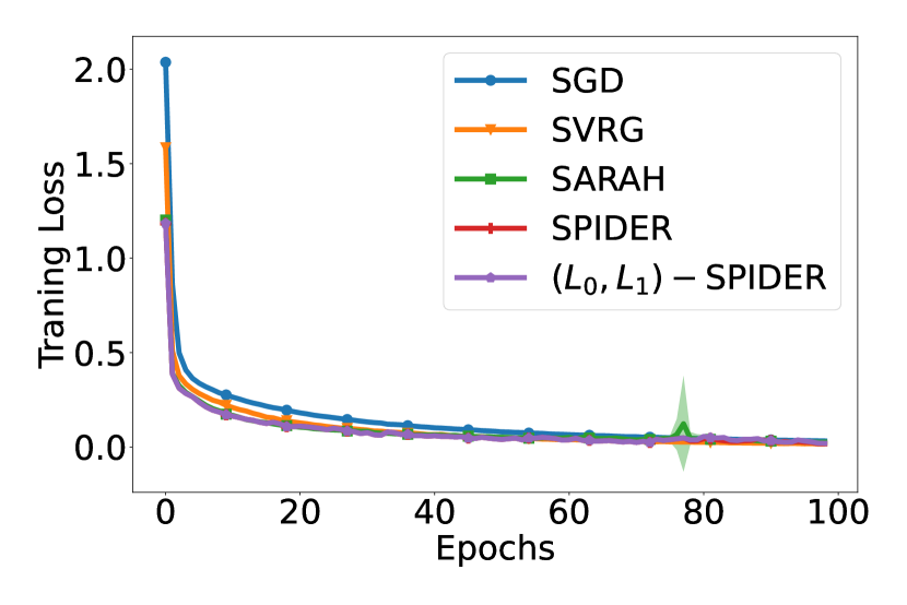
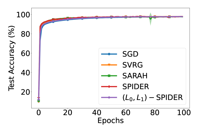
(a) FCN on MNIST

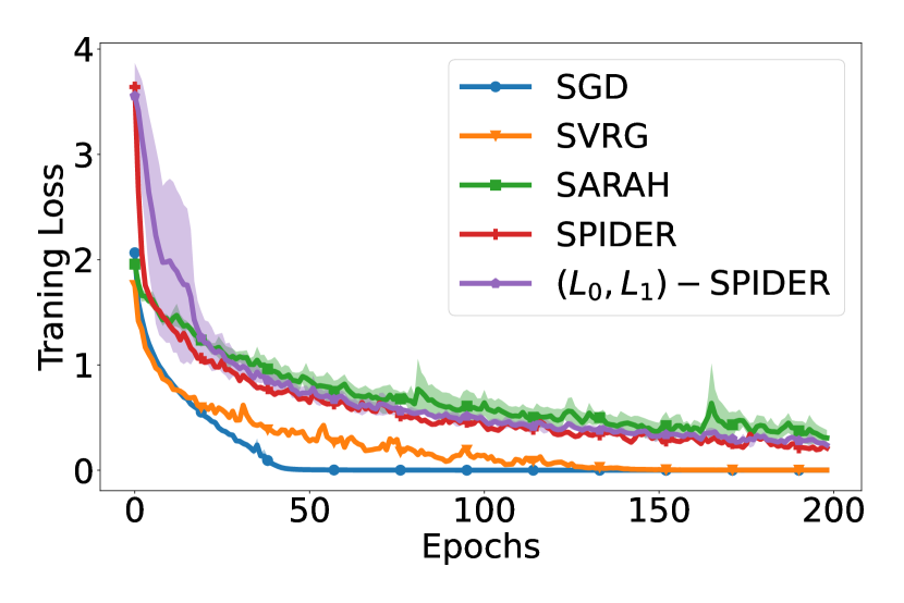
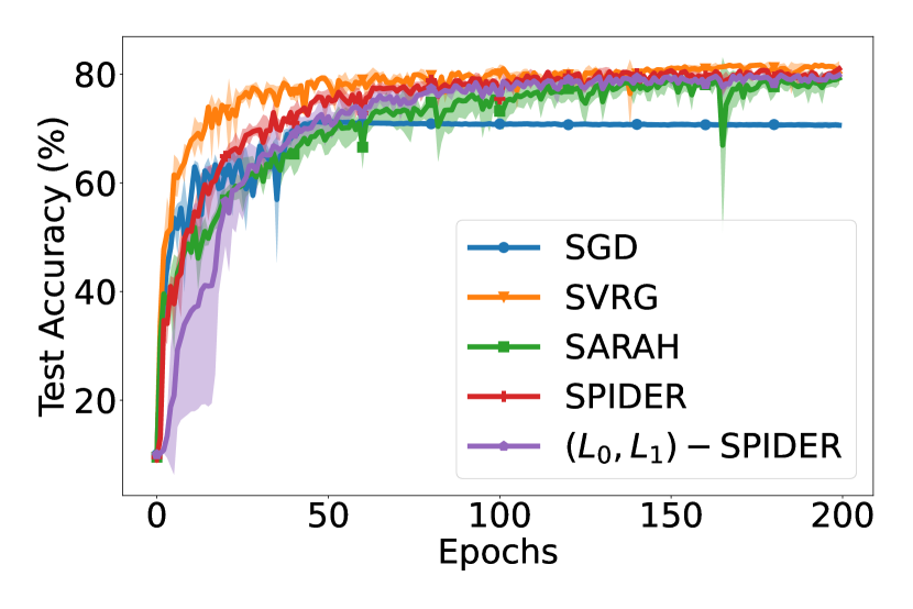
(b) ResNet-20 on CIFAR10

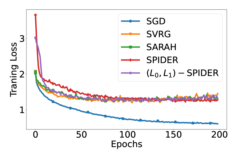
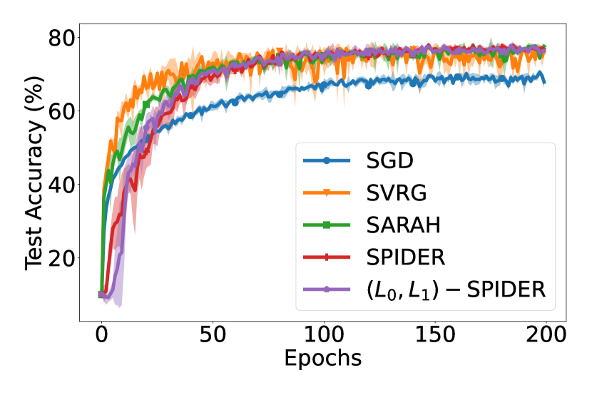
(c) ResNet-20 on noisy CIFAR10

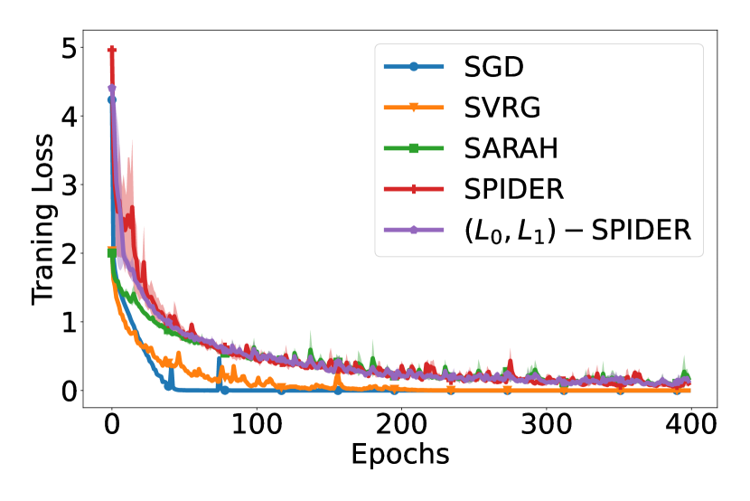
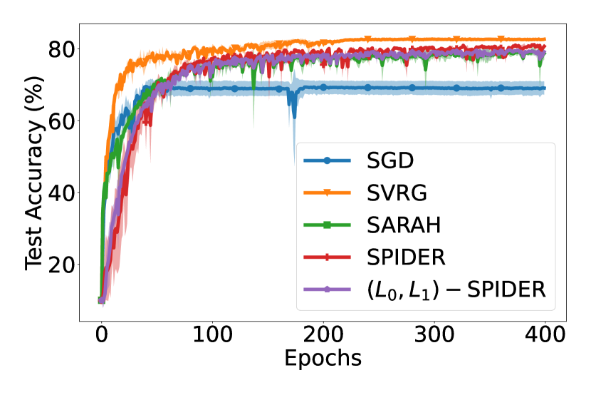
(d) ResNet-56 on CIFAR10

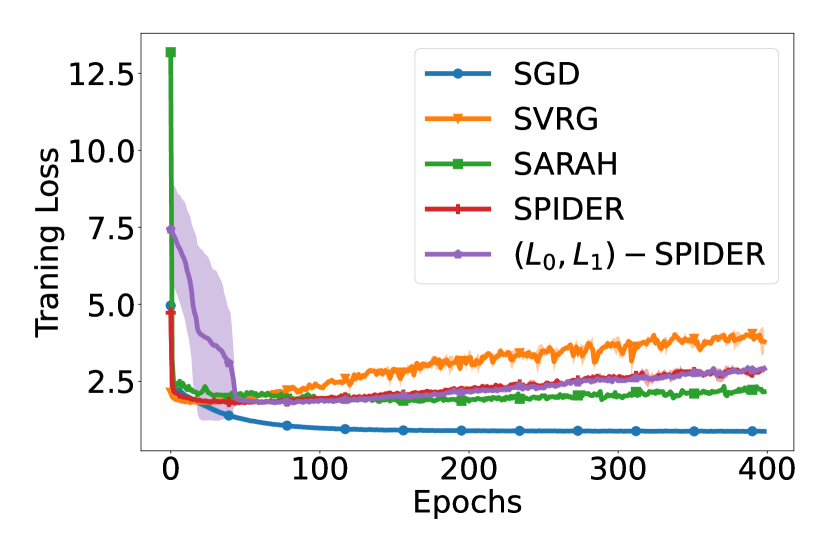
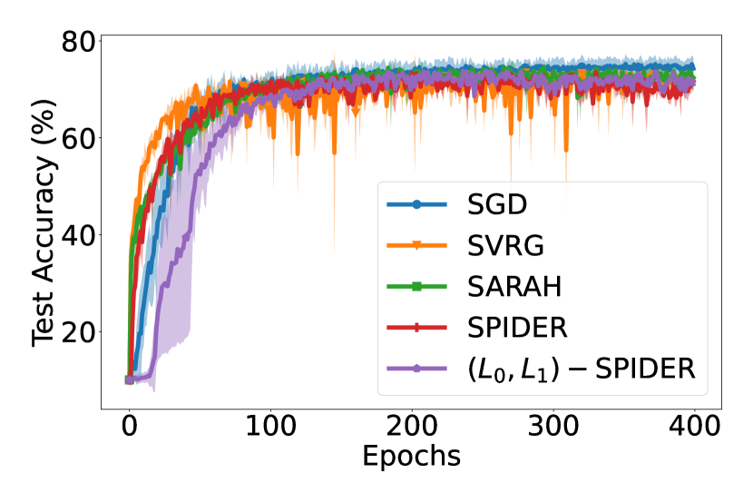
(e) ResNet-56 on noisy CIFAR10

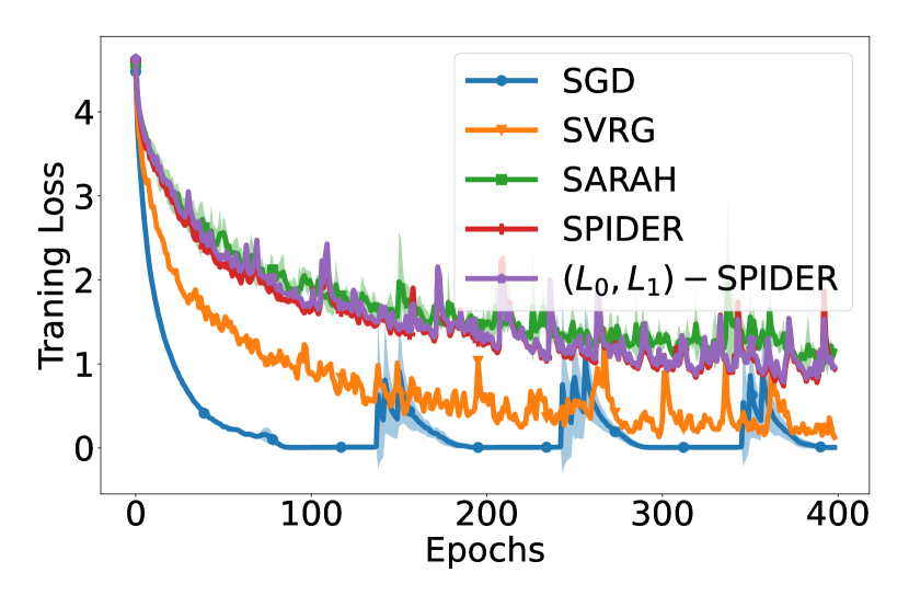
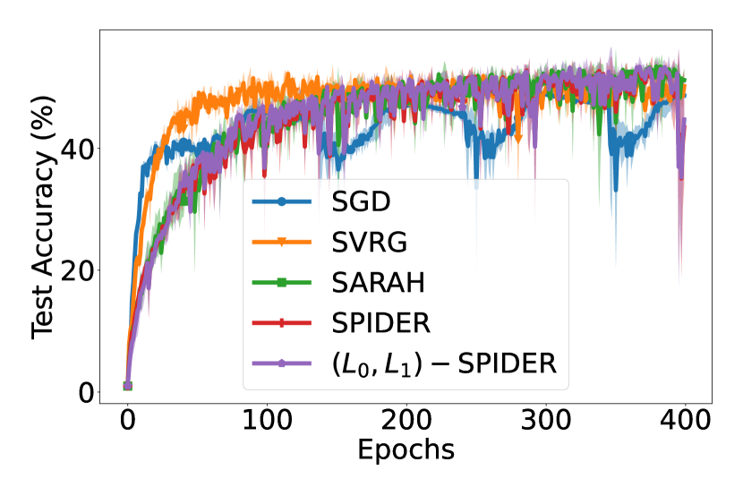
(f) ResNet-20 on CIFAR100

Figure 2: Image classification tasks with neural networks.

As demonstrated in Figure 2(2(a)), for the simple task of training FCN on MNIST, all methods achieve fairly high test accuracy and show almost identical performances. Figure 2(2(b)) provides training and test accuracy curves for ResNet-20 trained on clean (noiseless) CIFAR10. Although the test accuracy of Sgd is lower than that of variance reduction methods, it converges much faster during the training. This is in accordance with the conclusions in (Defazio and Bottou, 2019) that variance reduction methods are not very efficient for deep learning tasks. We highlight that our proposed $(L_{0},L_{1})$–Spider achieves similar performance to the original Spider, and the additional $\mathcal{O}(\|{\mathbf{v}}_{k}\|^{-2})$ term in the stepsize does not slow down the training much except in the initial steps. Quantitatively, $(L_{0},L_{1})$–Spider attains $79.94\%$ test accuracy which is comparable to other variance-reduced benchmarks with $81.72\%$, $79.28\%$ and $81.03\%$ test accuracy. We provide further quantitative results in the appendix.

We further train the same model on noisy CIFAR10. That is, we add Gaussian noise with zero-mean and unit-variance to the images and change the label with probability $0.1$ to all possible categories uniformly. As Figure 2(2(c)) shows, although Svrg is still slightly faster than other variance-reduced methods, both Spider and $(L_{0},L_{1})$–Spider achieve better test accuracy compared to the noiseless experiments in Figure 2(2(b)) which underscore the potential robustness of Spider to noise.

Next, we train a larger model, that is ResNet-56 on both noiseless and noisy CIFAR10 dataset. As depicted in Figures 2(2(d)) and 2(2(e)), $(L_{0},L_{1})$–Spider achieves similar performance to the other variance-reduced benchmarks. They also share other aspects in their convergence with those of the smaller model ResNet-20 in Figures 2(2(b)) and 2(2(c)). Finally, we use a more complicated task with CIFAR100 dataset and train ResNet-20 with results demonstrated in Figure 2(2(f)).

5 Conclusion

Gradient clipping has been extensively used in training deep neural networks for particular applications such as language models. The training trajectory of gradient clipping for such models contradicts the traditional $L$–smoothness assumption which calls for relaxing this premise in non-convex optimization. The more relaxed $(L_{0},L_{1})$–smooth notion has laid out a theoretical framework to study the performance and complexity of gradient clipping methods. In this work, we improved the gradient complexity of clipping methods under this broader setting by employing a variance reduction technique called Spider. We showed that Spider with a carefully picked learning rate is able to achieve the order-optimal gradient complexity rates in finding first-order stationary points. It however remains to study how this method can be boosted to escape from saddle points and find second-order stationary solutions for $(L_{0},L_{1})$–smooth non-convex objectives. Similar to the first-order literature, most of the existing works on the second-order methods highly utilize the restrictive Hessian Lipschitz assumption which most likely breaks in the $(L_{0},L_{1})$–smooth setting. We leave this direction for future work.

Appendices

Appendix A Experiment Setup

Here, we provide further details about our experiments along with quantitative illustrations of the results laid out in Figure 2 from the main paper.

As discussed in the main paper, we train three different neural networks, which are a three-layer fully connected network (FCN), ResNet-20 and ResNet-56 on several datasets, that are MNIST, CIFAR10 and CIFAR100. In each experiment, we compare the performance of $(L_{0},L_{1})$–Spider against benchmarks including Sgd, Svrg, Sarah and Spider. For each method, its hyper-parameters like learning rate are tuned over a range to achieve the best possible test accuracy. In addition to the datasets mentioned above, we conduct experiments on their noisy versions. In particular, we train ResNet-20 on a noisy CIFAR10 dataset. Here, we add Gaussian noise to the images from CIFAR10 dataset with variance $1$ in $\ell_{2}$ norm and also change the label with probability $0.1$ to all possible categories uniformly. Moreover, we double the noise scale on CIFAR10 and train ResNet-56 model. Figure 2 in the main paper demonstrates our results for the experiments described above where for each setting, we conduct three runs and show both mean and standard deviation. Furthermore, we provide quantitative implications from the same experiments in the following table. To obtain each entry in this table, we pick the best test accuracy along each of the three trajectories and report their average, as shown in Table 3. In the supplementary materials, we provide the code of our experiments which is modified from that of (Horváth et al., 2020).

Table 3: Test accuracy ($\%$) corresponding to experiments in Figure 2. ^∗Noisy data.

	FCN	ResNet-20			ResNet-56
Method	MNIST	CIFAR10	CIFAR10∗	CIFAR100	CIFAR10	CIFAR10∗
Sgd	$97.83$	$71.31$	$70.52$	$49.02$	$69.36$	$75.26$
Svrg	$97.98$	$81.72$	$77.00$	$52.24$	$82.76$	$73.49$
Sarah	$97.75$	$79.28$	$77.94$	$53.45$	$79.45$	$74.62$
Spider	$98.04$	$81.03$	$77.95$	$53.33$	$81.2$	$73.53$
$(L_{0},L_{1})$–Spider	$97.91$	$79.94$	$77.82$	$53.39$	$79.69$	$73.83$

Next, we provide the detailed hyper-parameters corresponding to all the curves in Figure 2. First, the mini-batch size for all the methods and datasets is fixed as $1024$. For Sgd, Svrg, and Sarah, the only hyper-parameter to tune is the learning rate $\eta_{0}$. However, for Spider, the stepsize at iteration $k$ is $\eta_{k}=\eta_{0}\min\{1,c_{1}/\|{\mathbf{v}}_{k}\|\}$ which is determined by the learning rate $\eta_{0}$ and the clipping parameter $c_{1}$. For $(L_{0},L_{1})$–Spider, the stepsize is $\eta_{k}=\eta_{0}\min\{1,c_{1}/\|{\mathbf{v}}_{k}\|,c_{2}/\|{\mathbf{v}}_{k}\|^{2}\}$ which is governed by the learning rate $\eta_{0}$ and two clipping parameters $c_{1}$ and $c_{2}$. All of the hyper-parameters are tuned to obtain the best test accuracy. We show the tuned learning rates for all experiments in Table 4. Moreover, Table 5 provides the tuned clipping parameters $c_{1}$ for Spider and $(c_{1},c_{2})$ for $(L_{0},L_{1})$–Spider methods. Note that we do not use techniques such as momentum or weight decay for any of our experiments except in training ResNet-20 on CIFAR100, for which we use a momentum parameter of $0.9$ and weight decay parameter of $10^{-4}$ to get a better test accuracy.

	FCN	ResNet-20			ResNet-56
Method	MNIST	CIFAR10	CIFAR10∗	CIFAR100	CIFAR10	CIFAR10∗
Sgd	$0.1$	$0.2$	$0.025$	$0.0125$	$0.2$	$1.6$
Svrg	$0.05$	$0.2$	$0.05$	$0.8$	$0.2$	$0.025$
Sarah	$0.025$	$0.05$	$0.025$	$0.025$	$0.0125$	$0.0125$
Spider	$0.0125$	$0.05$	$0.05$	$0.0125$	$0.025$	$0.0125$
$(L_{0},L_{1})$–Spider	$0.0125$	$0.025$	$0.025$	$0.05$	$0.0125$	$0.00625$

Table 4: Learning rates corresponding to experiments in Figure 2. ^∗Noisy data.

	FCN	ResNet-20			ResNet-56
Method	MNIST	CIFAR10	CIFAR10∗	CIFAR100	CIFAR10	CIFAR10∗
Spider	$0.5$	$1$	$0.5$	$16$	$8$	$16$
$(L_{0},L_{1})$–Spider	$(0.5,0.5)$	$(2,2)$	$(2,2)$	$(16,128)$	$(8,128)$	$(16,128)$

Table 5: Clipping parameters corresponding to experiments in Figure 2. ^∗Noisy data.

Appendix B Proof of Theorem 3

We first state and prove an essential lemma, a.k.a. the descent lemma, which is the common step in showing the convergence of non-convex optimization algorithms. Throughout this section, we use the notation $\mathbb{E}_{k}[\cdot]$ as the expectation conditioned on the history ${\mathcal{F}}_{k}$ containing $\{{\mathbf{x}}_{0\mathrel{\mathop{\mathchar 58\relax}}k},{\mathbf{v}}_{0\mathrel{\mathop{\mathchar 58\relax}}k-1}\}$.

Lemma 2 (Descent Lemma).

Assume that $F$ is $(L_{0},L_{1})$–smooth according to Definition 1 and consider the update ${\mathbf{x}}_{k+1}={\mathbf{x}}_{k}-\eta_{k}{\mathbf{v}}_{k}$. Then, for $\epsilon\leq\frac{L_{0}}{2L_{1}}$ and stepsize

$$\eta_{k}\leq\min\left\{\frac{1}{2L_{0}},\frac{\epsilon}{L_{0}\mathinner{\!\left\lVert{\mathbf{v}}_{k}\right\rVert}}\right\},$$ (20)

we have that for any iteration $k=0,1,\cdots$,

$$F({\mathbf{x}}_{k+1}) \leq F({\mathbf{x}}_{k})-\frac{1}{8}\eta_{k}\mathinner{\!\left\lVert{\mathbf{v}}_{k}\right\rVert}^{2}+\frac{5}{8}\eta_{k}\mathinner{\!\left\lVert{\mathbf{v}}_{k}-\nabla F({\mathbf{x}}_{k})\right\rVert}^{2}.$$ (21)

Proof. We defer the proof to Section F.2. $\square$

Another important step to show the convergence of variance reduction methods is to control the variance of the gradient estimator which is $\mathbb{E}\|{\mathbf{v}}_{k}-\nabla F({\mathbf{x}}_{k})\|^{2}$ in Algorithm 2. In the following lemma, we show that by scaling the stepsize inversely with both $\|{\mathbf{v}}_{k}\|$ and $\|{\mathbf{v}}_{k}\|^{2}$, we are able to control the variance $\mathbb{E}\|{\mathbf{v}}_{k}-\nabla F({\mathbf{x}}_{k})\|^{2}$.

Lemma 3.

Let Assumptions 1 (i) and 2 hold and assume that $\epsilon\leq\frac{L_{0}}{2L_{1}}$. Then, for stepsize and parameters picked as follows

$$\eta_{k}\leq\min\left\{\frac{1}{L_{0}}\frac{\epsilon}{\mathinner{\!\left\lVert{\mathbf{v}}_{k}\right\rVert}},\frac{1}{L_{1}}\frac{\epsilon}{\mathinner{\!\left\lVert{\mathbf{v}}_{k}\right\rVert}^{2}}\right\},$$ (22)

$$S_{1}=\frac{4\sigma^{2}}{\epsilon^{2}},\quad S_{2}=48\frac{L_{0}}{L_{1}}\frac{\sigma}{\epsilon},\quad q=2\frac{L_{0}}{L_{1}}\frac{\sigma}{\epsilon},$$ (23)

we have that

$$\mathbb{E}_{k_{0}}\Big{[}\mathinner{\!\left\lVert{\mathbf{v}}_{k}-\nabla F({\mathbf{x}}_{k})\right\rVert}^{2}\Big{]}\leq\epsilon^{2},$$ (24)

where $k_{0}\leq k$ denotes the most recent iterate to $k$ for which $q$ divides $k_{0}$, that is, $k_{0}=\lfloor k/q\rfloor\cdot q$.

Proof. We defer the proof to Section F.3. $\square$

Proof of Theorem 3: Having set up these two main helper lemmas, we move to prove Theorem 3. First, note that the specified choice of the stepsize and the accuracy condition $\epsilon<\frac{L_{0}}{20L_{1}}$ in Theorem 3 satisfy the ones required by Lemma 2. Therefore, using this lemma and the condition $\eta_{k}\leq 1/(2L_{0})$ we have that

$$F({\mathbf{x}}_{k+1}) \leq F({\mathbf{x}}_{k})-\frac{1}{8}\eta_{k}\mathinner{\!\left\lVert{\mathbf{v}}_{k}\right\rVert}^{2}+\frac{5}{8}\eta_{k}\mathinner{\!\left\lVert{\mathbf{v}}_{k}-\nabla F({\mathbf{x}}_{k})\right\rVert}^{2}\leq F({\mathbf{x}}_{k})-\frac{1}{8}\eta_{k}\mathinner{\!\left\lVert{\mathbf{v}}_{k}\right\rVert}^{2}+\frac{5}{16L_{0}}\mathinner{\!\left\lVert{\mathbf{v}}_{k}-\nabla F({\mathbf{x}}_{k})\right\rVert}^{2}.$$ (25)

Moreover, for the specified choice of the stepsize $\eta_{k}$, we have that

$$\eta_{k}\mathinner{\!\left\lVert{\mathbf{v}}_{k}\right\rVert}^{2} =\min\left\{\frac{\mathinner{\!\left\lVert{\mathbf{v}}_{k}\right\rVert}^{2}}{2L_{0}},\frac{\epsilon\mathinner{\!\left\lVert{\mathbf{v}}_{k}\right\rVert}}{L_{0}},\frac{\epsilon}{L_{1}}\right\}$$ (26)

$$=\min\left\{\frac{\epsilon^{2}}{L_{0}}\min\left\{\frac{1}{2}\mathinner{\!\left\lVert\frac{{\mathbf{v}}_{k}}{\epsilon}\right\rVert}^{2},\mathinner{\!\left\lVert\frac{{\mathbf{v}}_{k}}{\epsilon}\right\rVert}\right\},\frac{\epsilon}{L_{1}}\right\}$$ (27)

$$\overset{(a)}{\geq}\min\left\{\frac{\epsilon}{L_{0}}\mathinner{\!\left\lVert{\mathbf{v}}_{k}\right\rVert}-\frac{2\epsilon^{2}}{L_{0}},\frac{\epsilon}{L_{1}}\right\}$$ (28)

$$\geq\frac{\epsilon}{L_{0}}\min\left\{\mathinner{\!\left\lVert{\mathbf{v}}_{k}\right\rVert},\frac{L_{0}}{L_{1}}\right\}-\frac{2\epsilon^{2}}{L_{0}},$$ (29)

where in $(a)$, we used the inequality $\min\{x^{2}/2,|x|\}\geq|x|-2$ for all $x$. Rearranging terms in (25) combined with (26) yields that

$$\frac{\epsilon}{8L_{0}}\min\left\{\mathinner{\!\left\lVert{\mathbf{v}}_{k}\right\rVert},\frac{L_{0}}{L_{1}}\right\}-\frac{\epsilon^{2}}{4L_{0}}\leq F({\mathbf{x}}_{k})-F({\mathbf{x}}_{k+1})+\frac{5}{16L_{0}}\mathinner{\!\left\lVert{\mathbf{v}}_{k}-\nabla F({\mathbf{x}}_{k})\right\rVert}^{2}.$$ (30)

Next, we take expectations from both sides of the above inequality and use the bound in Lemma 3 which yields that

$$\frac{\epsilon}{8L_{0}}\mathbb{E}\left[\min\left\{\mathinner{\!\left\lVert{\mathbf{v}}_{k}\right\rVert},\frac{L_{0}}{L_{1}}\right\}\right]\leq\mathbb{E}[F({\mathbf{x}}_{k})]-\mathbb{E}[F({\mathbf{x}}_{k+1})]+\frac{9}{16L_{0}}\epsilon^{2}.$$ (31)

Now, we take the average of both sides over $k=0,\cdots,K-1$ which implies that

$$\frac{\epsilon}{8L_{0}}\cdot\frac{1}{K}\sum_{k=0}^{K-1}\mathbb{E}\left[\min\left\{\mathinner{\!\left\lVert{\mathbf{v}}_{k}\right\rVert},\frac{L_{0}}{L_{1}}\right\}\right]\leq\frac{F({\mathbf{x}}_{0})-\mathbb{E}[F({\mathbf{x}}_{K})]}{K}+\frac{9}{16L_{0}}\epsilon^{2}.$$ (32)

Multiplying both sides by $\frac{8L_{0}}{\epsilon}$ and using the fact that $F({\mathbf{x}}_{0})-\mathbb{E}[F({\mathbf{x}}_{K})]\leq F({\mathbf{x}}_{0})-F^{*}=\Delta$ yields that

$$\frac{1}{K}\sum_{k=0}^{K-1}\mathbb{E}\left[\min\left\{\mathinner{\!\left\lVert{\mathbf{v}}_{k}\right\rVert},\frac{L_{0}}{L_{1}}\right\}\right]\leq\frac{8\Delta L_{0}}{\epsilon K}+\frac{9}{2}\epsilon\leq 5\epsilon,$$ (33)

where we employed the following choice of the number of iterations

$$K=\bigg{\lceil}\frac{16\Delta L_{0}}{\epsilon^{2}}\bigg{\rceil}.$$ (34)

Now, consider index $\tilde{k}$ uniformly picked from $\{0,\cdots,K-1\}$ at random. The average argument in (33) implies that

$$\mathbb{E}\left[\min\left\{\mathinner{\!\left\lVert{\mathbf{v}}_{\tilde{k}}\right\rVert},\frac{L_{0}}{L_{1}}\right\}\right]\leq 5\epsilon,$$ (35)

where the expectation is w.r.t the randomness in both $\tilde{k}$ and the algorithm. Next, we use Markov’s inequality to yield that with probability at least $3/4$, we have

$$\min\left\{\mathinner{\!\left\lVert{\mathbf{v}}_{\tilde{k}}\right\rVert},\frac{L_{0}}{L_{1}}\right\}\leq 20\epsilon.$$ (36)

Note that for $\epsilon<\frac{L_{0}}{20L_{1}}$, we have $L_{0}/L_{1}<20\epsilon$. Therefore, the above bound simplifies to $\mathinner{\!\left\lVert{\mathbf{v}}_{\tilde{k}}\right\rVert}\leq 20\epsilon$.

Next, we have from Lemma 3 that $\mathbb{E}[\|{\mathbf{v}}_{k}-\nabla F({\mathbf{x}}_{k})\|^{2}]\leq\epsilon^{2}$ for every $k$. For uniformly picked $\tilde{k}\in\{0,\cdots,K-1\}$ we have

$$\mathbb{E}\left[\|{\mathbf{v}}_{\tilde{k}}-\nabla F({\mathbf{x}}_{\tilde{k}})\|^{2}\right]=\frac{1}{K}\sum_{k=0}^{K-1}\mathbb{E}\left[\big{\|}{\mathbf{v}}_{k}-\nabla F({\mathbf{x}}_{k})\big{\|}^{2}\right]\leq\epsilon^{2},$$ (37)

which together with Jensen’s inequality implies that $\mathbb{E}\|{\mathbf{v}}_{\tilde{k}}-\nabla F({\mathbf{x}}_{\tilde{k}})\|\leq\epsilon$. Using Markov’s inequality, we have $\|{\mathbf{v}}_{\tilde{k}}-\nabla F({\mathbf{x}}_{\tilde{k}})\|\leq 4\epsilon$ with probability $3/4$. Finally, we use union bound on the above two good events to conclude that for randomly and uniformly picked index $\tilde{k}\in\{0,\cdots,K-1\}$,

$$\mathinner{\!\left\lVert\nabla F({\mathbf{x}}_{\tilde{k}})\right\rVert}\leq\mathinner{\!\left\lVert{\mathbf{v}}_{\tilde{k}}\right\rVert}+\mathinner{\!\left\lVert{\mathbf{v}}_{\tilde{k}}-\nabla F({\mathbf{x}}_{\tilde{k}})\right\rVert}\leq 20\epsilon+4\epsilon=24\epsilon,$$ (38)

with probability at least $1-1/4-1/4=1/2$.

Total iteration complexity: The total gradient complexity of Spider in Algorithm 2 can be bounded as follows

$$\bigg{\lceil}K\cdot\frac{1}{q}\bigg{\rceil}S_{1}+KS_{2} \leq K\cdot\frac{1}{q}\cdot S_{1}+S_{1}+KS_{2}$$ (39)

$$\leq\left(\frac{16\Delta L_{0}}{\epsilon^{2}}+1\right)\frac{L_{1}\epsilon}{2L_{0}\sigma}\cdot\frac{4\sigma^{2}}{\epsilon^{2}}+\frac{4\sigma^{2}}{\epsilon^{2}}+\left(\frac{16\Delta L_{0}}{\epsilon^{2}}+1\right)\frac{48L_{0}\sigma}{L_{1}\epsilon}$$ (40)

$$=32\Delta\sigma\left(L_{1}+24\frac{L_{0}^{2}}{L_{1}}\right)\frac{1}{\epsilon^{3}}+\frac{4\sigma^{2}}{\epsilon^{2}}+2\sigma\left(\frac{L_{1}}{L_{0}}+24\frac{L_{0}}{L_{1}}\right)\frac{1}{\epsilon}.$$ (41)

Appendix C Proof of Theorem 4

Before proving Theorem 4 which corresponds to the finite-sum setting, we provide two helper lemmas. First, Lemma 2 can be directly employed in the finite-sum setting, as well as the stochastic setting. Second, we bound the variance $\mathbb{E}\|{\mathbf{v}}_{k}-\nabla F({\mathbf{x}}_{k})\|^{2}$ in the finite-sum setting, similar to Lemma 3 in the stochastic setting.

Lemma 4.

Let Assumption 1 (ii) hold and assume that $\epsilon\leq\frac{L_{0}}{2L_{1}}$. Then, for stepsize and parameters picked as follows

$$\eta_{k}\leq\min\left\{\frac{1}{L_{0}}\frac{\epsilon}{\mathinner{\!\left\lVert{\mathbf{v}}_{k}\right\rVert}},\frac{1}{L_{1}}\frac{\epsilon}{\mathinner{\!\left\lVert{\mathbf{v}}_{k}\right\rVert}^{2}}\right\}$$ (42)

$$S_{1}=n,\quad S_{2}=12\sqrt{n},\quad q=\sqrt{n},$$ (43)

we have that

$$\mathbb{E}_{k_{0}}\Big{[}\mathinner{\!\left\lVert{\mathbf{v}}_{k}-\nabla F({\mathbf{x}}_{k})\right\rVert}^{2}\Big{]}\leq\epsilon^{2},$$ (44)

where $k_{0}\leq k$ denotes the most recent iterate to $k$ for which $q$ divides $k_{0}$, that is, $k_{0}=\lfloor k/q\rfloor\cdot q$.

Proof. We defer the proof to Section F.4. $\square$

Proof of Theorem 4: Using the descent lemma in Lemma 2 and the variance bound established in Lemma 4, the rest of the proof follows from the proof of Theorem 3. Particularly, for randomly and uniformly picked index ${\tilde{k}}\in\{0,\cdots,K-1\}$, we have $\|\nabla F({\mathbf{x}}_{\tilde{k}})\|\leq 24\epsilon$ with probability at least $1/2$. The total iteration complexity of finding such a stationary point is bounded by

$$\bigg{\lceil}K\cdot\frac{1}{q}\bigg{\rceil}S_{1}+KS_{2} \leq K\cdot\frac{1}{q}\cdot S_{1}+S_{1}+KS_{2}$$ (45)

$$\leq\left(\frac{16\Delta L_{0}}{\epsilon^{2}}+1\right)\frac{1}{\sqrt{n}}\cdot n+n+\left(\frac{16\Delta L_{0}}{\epsilon^{2}}+1\right)12\sqrt{n}$$ (46)

$$=208\Delta L_{0}\sqrt{n}\frac{1}{\epsilon^{2}}+n+13\sqrt{n}.$$ (47)

Appendix D Proof of Theorem 1

We first employ the Descent Lemma (Lemma 2 and treating ${\mathbf{v}}_{k}$ as stochastic gradient ${\mathbf{g}}_{k}$) which implies that

$$F({\mathbf{x}}_{k+1})\leq F({\mathbf{x}}_{k})-\frac{1}{8}\eta_{k}\mathinner{\!\left\lVert{\mathbf{g}}_{k}\right\rVert}^{2}+\frac{5}{16L_{0}}\mathinner{\!\left\lVert{\mathbf{g}}_{k}-\nabla F({\mathbf{x}}_{k})\right\rVert}^{2}.$$ (48)

Next, for the specified choice of stepsize $\eta_{k}$, we can write that

$$\eta_{k}\mathinner{\!\left\lVert{\mathbf{g}}_{k}\right\rVert}^{2} =\min\left\{\frac{\mathinner{\!\left\lVert{\mathbf{g}}_{k}\right\rVert}^{2}}{2L_{0}},\frac{\epsilon\mathinner{\!\left\lVert{\mathbf{g}}_{k}\right\rVert}}{L_{0}}\right\}$$ (49)

$$=\frac{\epsilon^{2}}{L_{0}}\min\left\{\frac{1}{2}\mathinner{\!\left\lVert\frac{{\mathbf{g}}_{k}}{\epsilon}\right\rVert}^{2},\mathinner{\!\left\lVert\frac{{\mathbf{g}}_{k}}{\epsilon}\right\rVert}\right\}$$ (50)

$$\overset{(a)}{\geq}\frac{\epsilon}{L_{0}}\mathinner{\!\left\lVert{\mathbf{g}}_{k}\right\rVert}-\frac{2\epsilon^{2}}{L_{0}},$$ (51)

where $(a)$ follows from the fact that $\min\{x^{2}/2,|x|\}\geq|x|-2$ for all $x$. Plugging this back into (58) yields that

$$\frac{\epsilon}{8L_{0}}\mathinner{\!\left\lVert{\mathbf{g}}_{k}\right\rVert}-\frac{\epsilon^{2}}{4L_{0}}\leq F({\mathbf{x}}_{k})-F({\mathbf{x}}_{k+1})+\frac{5}{16L_{0}}\mathinner{\!\left\lVert{\mathbf{g}}_{k}-\nabla F({\mathbf{x}}_{k})\right\rVert}^{2}.$$ (52)

We take expectation from both sides of the above which together with $\mathbb{E}\|{\mathbf{g}}_{k}-\nabla F({\mathbf{x}}_{k})\|^{2}\leq\frac{\sigma^{2}}{S}$ yields that

$$\mathbb{E}\mathinner{\!\left\lVert{\mathbf{g}}_{k}\right\rVert}\leq\frac{8L_{0}}{\epsilon}\left(\mathbb{E}[F({\mathbf{x}}_{k})]-\mathbb{E}[F({\mathbf{x}}_{k+1})]\right)+\frac{5}{2\epsilon}\cdot\frac{\sigma^{2}}{S}+2\epsilon.$$ (53)

Next, we sum the above inequality over $k=0,\cdots,K-1$ and conclude that

$$\frac{1}{K}\sum_{k=0}^{K-1}\mathbb{E}\mathinner{\!\left\lVert{\mathbf{g}}_{k}\right\rVert}\leq\frac{8\Delta L_{0}}{\epsilon K}+\frac{5}{2\epsilon}\cdot\frac{\sigma^{2}}{S}+2\epsilon\leq\frac{\epsilon}{2}+\frac{5}{2}\epsilon+2\epsilon=5\epsilon,$$ (54)

where we used the parameter choices

$$S=\frac{\sigma^{2}}{\epsilon^{2}},\quad K=\bigg{\lceil}\frac{16\Delta L_{0}}{\epsilon^{2}}\bigg{\rceil}.$$ (55)

Now, consider index $\tilde{k}$ uniformly picked from $\{0,\cdots,K-1\}$ at random. The average argument in (54) implies that $\mathbb{E}\|{\mathbf{g}}_{\tilde{k}}\|\leq 5\epsilon$ where the expectation is w.r.t the randomness in both $\tilde{k}$ and the algorithm. Moreover, the variance of the stochastic gradient ${\mathbf{g}}_{k}$ is bounded by $\mathbb{E}\|{\mathbf{g}}_{k}-\nabla F({\mathbf{x}}_{k})\|^{2}\leq\frac{\sigma^{2}}{S}=\epsilon^{2}$ for every $k$, which together with Jensen’s inequality yields that $\mathbb{E}\|{\mathbf{g}}_{\tilde{k}}-\nabla F({\mathbf{x}}_{\tilde{k}})\|\leq\epsilon$. Therefore, we can write

$$\mathbb{E}\mathinner{\!\left\lVert\nabla F({\mathbf{x}}_{\tilde{k}})\right\rVert}\leq\mathbb{E}\mathinner{\!\left\lVert{\mathbf{g}}_{\tilde{k}}\right\rVert}+\mathbb{E}\mathinner{\!\left\lVert{\mathbf{g}}_{\tilde{k}}-\nabla F({\mathbf{x}}_{\tilde{k}})\right\rVert}\leq 6\epsilon.$$ (56)

Finally, we use Markov’s inequality to conclude that for randomly and uniformly picked index ${\tilde{k}}\in\{0,\cdots,K-1\}$, we have $\|\nabla F({\mathbf{x}}_{\tilde{k}})\|\leq 12\epsilon$ with probability at least $1/2$.

Total gradient complexity can be bounded as follows

$$KS\leq\left(\frac{16\Delta L_{0}}{\epsilon^{2}}+1\right)\frac{\sigma^{2}}{\epsilon^{2}}=16\Delta L_{0}\sigma^{2}\frac{1}{\epsilon^{4}}+\frac{\sigma^{2}}{\epsilon^{2}}.$$ (57)

Appendix E Proof of Theorem 2

First, note that when using the full batch ($S=n$), we have ${\mathbf{g}}_{k}=\nabla F({\mathbf{x}}_{k})$. Using the Descent Lemma (Lemma 2 and treating ${\mathbf{v}}_{k}=\nabla F({\mathbf{x}}_{k})$), we have that

$$F({\mathbf{x}}_{k+1})\leq F({\mathbf{x}}_{k})-\frac{1}{8}\eta_{k}\mathinner{\!\left\lVert\nabla F({\mathbf{x}}_{k})\right\rVert}^{2}.$$ (58)

Next, following the same argument as in (49), we have that

$$\frac{\epsilon}{8L_{0}}\mathinner{\!\left\lVert\nabla F({\mathbf{x}}_{k})\right\rVert}-\frac{\epsilon^{2}}{4L_{0}}\leq F({\mathbf{x}}_{k})-F({\mathbf{x}}_{k+1}).$$ (59)

Summing over $k=0,\cdots,K-1$ yields that

$$\frac{1}{K}\sum_{k=0}^{K-1}\mathinner{\!\left\lVert\nabla F({\mathbf{x}}_{k})\right\rVert}\leq\frac{8\Delta L_{0}}{\epsilon K}+2\epsilon\leq\frac{\epsilon}{2}+2\epsilon=\frac{5}{2}\epsilon.$$ (60)

Let iterate ${\tilde{k}}$ be uniformly picked from $\{0,\cdots,K-1\}$ at random. The average argument above implies that $\mathbb{E}\|\nabla F({\mathbf{x}}_{\tilde{k}})\|\leq\frac{5}{2}\epsilon$ which together with Markov’s inequality implies that $\|\nabla F({\mathbf{x}}_{\tilde{k}})\|\leq 5\epsilon$ with probability at least $1/2$.

Total gradient complexity can be bounded as follows

$$KS\leq\left(\frac{16\Delta L_{0}}{\epsilon^{2}}+1\right)n=16\Delta L_{0}n\frac{1}{\epsilon^{2}}+n.$$ (61)

Appendix F Proof of Deferred Lemmas

F.1 Proof of Proposition 1

Let condition (5) hold. Then, for any unit-norm vector ${\mathbf{u}}$, we have that

$$\mathinner{\!\left\lVert\nabla^{2}F({\mathbf{x}}){\mathbf{u}}\right\rVert}=\Big{\|}\lim_{t\to 0}\frac{1}{t}\left(\nabla F({\mathbf{x}}+t{\mathbf{u}})-\nabla F({\mathbf{x}})\right)\Big{\|}=\lim_{t\to 0}\frac{1}{t}\mathinner{\!\left\lVert\nabla F({\mathbf{x}}+t{\mathbf{u}})-\nabla F({\mathbf{x}})\right\rVert}\leq L_{0}+L_{1}\|\nabla F({\mathbf{x}})\|.$$ (62)

Therefore, we have $\|\nabla^{2}F({\mathbf{x}})\|=\sup_{\|{\mathbf{u}}\|=1}\|\nabla^{2}F({\mathbf{x}}){\mathbf{u}}\|\leq L_{0}+L_{1}\|\nabla F({\mathbf{x}})\|$, which is the same as condition (4). The other direction is a special case of the following result proved in (Zhang et al., 2020).

Lemma 5 (Corollary A.4 in Zhang et al. (2020)).

Assume that $F$ satisfies (4), that is, $\|\nabla^{2}F({\mathbf{x}})\|\leq L_{0}+L_{1}\|\nabla F({\mathbf{x}})\|$ for all ${\mathbf{x}}$. For any $c>0$, if $\|{\mathbf{x}}-{\mathbf{y}}\|\leq c/L_{1}$, then

$$\|\nabla F({\mathbf{x}})-\nabla F({\mathbf{y}})\|\leq\big{(}AL_{0}+BL_{1}\|\nabla F({\mathbf{x}})\|\big{)}\|{\mathbf{x}}-{\mathbf{y}}\|,$$ (63)

where $A=1+e^{c}-\frac{e^{c}-1}{c}$ and $B=\frac{e^{c}-1}{c}$.

Taking $c=1$ in the above lemma yields that $A=2$ and $B=e-1\leq 2$. Therefore, condition (5) holds with $2L_{0}$ and $2L_{1}$.

F.2 Proof of Lemma 2

Consider any iteration $k$ and define ${\mathbf{x}}(t)=t({\mathbf{x}}_{k+1}-{\mathbf{x}}_{k})+{\mathbf{x}}_{k}$ for any $t\in[0,1]$ which lies between ${\mathbf{x}}_{k}$ and ${\mathbf{x}}_{k+1}$. From Taylor’s Theorem, we have that

$$F({\mathbf{x}}_{k+1}) =F({\mathbf{x}}_{k})+\int_{0}^{1}\langle\nabla F({\mathbf{x}}(t)),{\mathbf{x}}_{k+1}-{\mathbf{x}}_{k}\rangle dt$$ (64)

$$=F({\mathbf{x}}_{k})+\langle\nabla F({\mathbf{x}}_{k}),{\mathbf{x}}_{k+1}-{\mathbf{x}}_{k}\rangle+\int_{0}^{1}\langle\nabla F({\mathbf{x}}(t))-\nabla F({\mathbf{x}}_{k}),{\mathbf{x}}_{k+1}-{\mathbf{x}}_{k}\rangle\mathop{}\!\mathrm{d}t$$ (65)

$$\overset{(a)}{\leq}F({\mathbf{x}}_{k})+\langle\nabla F({\mathbf{x}}_{k}),{\mathbf{x}}_{k+1}-{\mathbf{x}}_{k}\rangle+\int_{0}^{1}\left(L_{0}+L_{1}\|\nabla F({\mathbf{x}}_{k})\|\right)\|{\mathbf{x}}_{k+1}-{\mathbf{x}}_{k}\|^{2}t\,\mathop{}\!\mathrm{d}t$$ (66)

$$=F({\mathbf{x}}_{k})+\langle\nabla F({\mathbf{x}}_{k}),{\mathbf{x}}_{k+1}-{\mathbf{x}}_{k}\rangle+\frac{1}{2}\left(L_{0}+L_{1}\|\nabla F({\mathbf{x}}_{k})\|\right)\|{\mathbf{x}}_{k+1}-{\mathbf{x}}_{k}\|^{2},$$ (67)

where in $(a)$ we used Definition 1 since $\|{\mathbf{x}}(t)-{\mathbf{x}}_{k}\|\leq\|{\mathbf{x}}_{k+1}-{\mathbf{x}}_{k}\|=\eta_{k}\|{\mathbf{v}}_{k}\|\leq\epsilon/L_{0}\leq 1/(2L_{1})\leq 1/L_{1}$. We can continue bounding $F({\mathbf{x}}_{k+1})$ by replacing ${\mathbf{x}}_{k+1}-{\mathbf{x}}_{k}=-\eta_{k}{\mathbf{v}}_{k}$ in (64) as follows

$$F({\mathbf{x}}_{k+1}) \leq F({\mathbf{x}}_{k})-\eta_{k}\langle\nabla F({\mathbf{x}}_{k}),{\mathbf{v}}_{k}\rangle+\frac{1}{2}L_{0}\eta_{k}^{2}\|{\mathbf{v}}_{k}\|^{2}+\frac{1}{2}L_{1}\eta_{k}^{2}\|{\mathbf{v}}_{k}\|^{2}\|\nabla F({\mathbf{x}}_{k})\|$$ (68)

$$\leq F({\mathbf{x}}_{k})-\eta_{k}\langle\nabla F({\mathbf{x}}_{k}),{\mathbf{v}}_{k}\rangle+\frac{1}{2}L_{0}\eta_{k}^{2}\|{\mathbf{v}}_{k}\|^{2}+\frac{1}{4}L_{1}\eta_{k}^{2}\|{\mathbf{v}}_{k}\|^{3}+\frac{1}{4}L_{1}\eta_{k}^{2}\|{\mathbf{v}}_{k}\|\cdot\mathinner{\!\left\lVert{\mathbf{v}}_{k}-\nabla F({\mathbf{x}}_{k})\right\rVert}^{2}$$ (69)

$$\leq F({\mathbf{x}}_{k})-\frac{1}{2}\eta_{k}\left(1-L_{0}\eta_{k}\right)\mathinner{\!\left\lVert{\mathbf{v}}_{k}\right\rVert}^{2}+\frac{1}{4}L_{1}\eta_{k}^{2}\|{\mathbf{v}}_{k}\|^{3}+\frac{1}{2}\eta_{k}\mathinner{\!\left\lVert{\mathbf{v}}_{k}-\nabla F({\mathbf{x}}_{k})\right\rVert}^{2}$$ (70)

$$\quad+\frac{1}{4}L_{1}\eta_{k}^{2}\|{\mathbf{v}}_{k}\|\cdot\mathinner{\!\left\lVert{\mathbf{v}}_{k}-\nabla F({\mathbf{x}}_{k})\right\rVert}^{2}$$ (71)

$$\overset{(b)}{\leq}F({\mathbf{x}}_{k})-\frac{1}{4}\eta_{k}\mathinner{\!\left\lVert{\mathbf{v}}_{k}\right\rVert}^{2}+\frac{1}{8}\eta_{k}\|{\mathbf{v}}_{k}\|^{2}+\frac{1}{2}\eta_{k}\mathinner{\!\left\lVert{\mathbf{v}}_{k}-\nabla F({\mathbf{x}}_{k})\right\rVert}^{2}+\frac{1}{8}\eta_{k}\mathinner{\!\left\lVert{\mathbf{v}}_{k}-\nabla F({\mathbf{x}}_{k})\right\rVert}^{2}$$ (72)

$$=F({\mathbf{x}}_{k})-\frac{1}{8}\eta_{k}\mathinner{\!\left\lVert{\mathbf{v}}_{k}\right\rVert}^{2}+\frac{5}{8}\eta_{k}\mathinner{\!\left\lVert{\mathbf{v}}_{k}-\nabla F({\mathbf{x}}_{k})\right\rVert}^{2}.$$ (73)

In deriving $(b)$ above, we particularly used the conditions $L_{0}\eta_{k}\leq 1/2$ and $\eta_{k}\|{\mathbf{v}}_{k}\|\leq\epsilon/L_{0}\leq 1/(2L_{1})$ on the step-size.

F.3 Proof of Lemma 3

Consider iterate $k=0,1,\cdots$ and let us denote by $k_{0}\leq k$ the most recent iterate to $k$ for which $q$ divides $k_{0}$, that is, $k_{0}=\lfloor k/q\rfloor\cdot q$. This implies that Spider updates ${\mathbf{v}}_{k_{0}}=\nabla f({\mathbf{x}}_{k_{0}};{\mathcal{S}}_{1})$ (Algorithm 2). Therefore, for $k=k_{0}$, we have that

$$\mathbb{E}_{k_{0}}\Big{[}\mathinner{\!\left\lVert{\mathbf{v}}_{k_{0}}-\nabla F({\mathbf{x}}_{k_{0}})\right\rVert}^{2}\Big{]}=\mathbb{E}_{k_{0}}\Big{[}\mathinner{\!\left\lVert\nabla f({\mathbf{x}}_{k_{0}};{\mathcal{S}}_{1})-\nabla F({\mathbf{x}}_{k_{0}})\right\rVert}^{2}\Big{]}\leq\frac{\sigma^{2}}{S_{1}}=\frac{\epsilon^{2}}{4}.$$ (74)

For any $k_{0}\leq k<k_{0}+q$, we have

$$\mathbb{E}\Big{[}\mathinner{\!\left\lVert{\mathbf{v}}_{k+1}-\nabla F({\mathbf{x}}_{k+1})\right\rVert}^{2}|\,{\mathcal{F}}_{k+1}\Big{]} =\mathbb{E}\Big{[}\mathinner{\!\left\lVert\nabla f({\mathbf{x}}_{k+1};{\mathcal{S}}_{2})-\nabla f({\mathbf{x}}_{k};{\mathcal{S}}_{2})+{\mathbf{v}}_{k}-\nabla F({\mathbf{x}}_{k+1})\right\rVert}^{2}|\,{\mathcal{F}}_{k+1}\Big{]}$$ (75)

$$=\mathbb{E}\Big{[}\mathinner{\!\left\lVert\nabla f({\mathbf{x}}_{k+1};{\mathcal{S}}_{2})-\nabla f({\mathbf{x}}_{k};{\mathcal{S}}_{2})+\nabla F({\mathbf{x}}_{k})-\nabla F({\mathbf{x}}_{k+1})\right\rVert}^{2}|\,{\mathcal{F}}_{k+1}\Big{]}$$ (76)

$$\quad+\mathinner{\!\left\lVert{\mathbf{v}}_{k}-\nabla F({\mathbf{x}}_{k})\right\rVert}^{2}.$$ (77)

Noting that the mini-batch ${\mathcal{S}}_{2}$ is of size $|{\mathcal{S}}_{2}|=S_{2}$, the first term in RHS of above can be bounded as follows

$$\quad\mathbb{E}\Big{[}\mathinner{\!\left\lVert\nabla f({\mathbf{x}}_{k+1};{\mathcal{S}}_{2})-\nabla f({\mathbf{x}}_{k};{\mathcal{S}}_{2})+\nabla F({\mathbf{x}}_{k})-\nabla F({\mathbf{x}}_{k+1})\right\rVert}^{2}|\,{\mathcal{F}}_{k+1}\Big{]}$$ (78)

$$\leq\frac{1}{S_{2}}\mathbb{E}\Big{[}\mathinner{\!\left\lVert\nabla f({\mathbf{x}}_{k+1};\xi)-\nabla f({\mathbf{x}}_{k};\xi)\right\rVert}^{2}|\,{\mathcal{F}}_{k+1}\Big{]}$$ (79)

$$\leq\frac{1}{S_{2}}\left(L_{0}+L_{1}\mathinner{\!\left\lVert\nabla F({\mathbf{x}}_{k})\right\rVert}\right)^{2}\mathinner{\!\left\lVert{\mathbf{x}}_{k+1}-{\mathbf{x}}_{k}\right\rVert}^{2}$$ (80)

$$\leq\frac{2}{S_{2}}L_{0}\eta_{k}^{2}\mathinner{\!\left\lVert{\mathbf{v}}_{k}\right\rVert}^{2}+\frac{2}{S_{2}}L_{1}^{2}\eta_{k}^{2}\mathinner{\!\left\lVert{\mathbf{v}}_{k}\right\rVert}^{2}\cdot\mathinner{\!\left\lVert\nabla F({\mathbf{x}}_{k})\right\rVert}^{2}$$ (81)

$$\leq\frac{2}{S_{2}}L_{0}^{2}\eta_{k}^{2}\mathinner{\!\left\lVert{\mathbf{v}}_{k}\right\rVert}^{2}+\frac{4}{S_{2}}L_{1}^{2}\eta_{k}^{2}\mathinner{\!\left\lVert{\mathbf{v}}_{k}\right\rVert}^{4}+\frac{4}{S_{2}}L_{1}^{2}\eta_{k}^{2}\mathinner{\!\left\lVert{\mathbf{v}}_{k}\right\rVert}^{2}\cdot\mathinner{\!\left\lVert{\mathbf{v}}_{k}-\nabla F({\mathbf{x}}_{k})\right\rVert}^{2}$$ (82)

$$\leq\frac{6}{S_{2}}\epsilon^{2}+\frac{4}{S_{2}}\left(\frac{L_{1}}{L_{0}}\right)^{2}\epsilon^{2}\mathinner{\!\left\lVert{\mathbf{v}}_{k}-\nabla F({\mathbf{x}}_{k})\right\rVert}^{2}.$$ (83)

In deriving the last inequality above, we used the facts that $L_{0}\eta_{k}\|{\mathbf{v}}_{k}\|\leq\epsilon$ and $L_{1}\eta_{k}\|{\mathbf{v}}_{k}\|^{2}\leq\epsilon$. Putting (75) and (78) together yields that

$$\mathbb{E}\Big{[}\mathinner{\!\left\lVert{\mathbf{v}}_{k+1}-\nabla F({\mathbf{x}}_{k+1})\right\rVert}^{2}|\,{\mathcal{F}}_{k+1}\Big{]} \leq\left(1+\frac{4}{S_{2}}\left(\frac{L_{1}}{L_{0}}\right)^{2}\epsilon^{2}\right)\mathinner{\!\left\lVert{\mathbf{v}}_{k}-\nabla F({\mathbf{x}}_{k})\right\rVert}^{2}+\frac{6}{S_{2}}\epsilon^{2}.$$ (84)

Let us take expectation from both sides of the above inequality w.r.t all the sources of randomness contained in $\{{\mathbf{x}}_{k_{0}+1\mathrel{\mathop{\mathchar 58\relax}}k+1},{\mathbf{v}}_{k_{0}\mathrel{\mathop{\mathchar 58\relax}}k}\}$ conditioned on ${\mathcal{F}}_{k_{0}}$. We also denote $e_{k}\coloneqq\mathbb{E}[\|{\mathbf{v}}_{k}-\nabla F({\mathbf{x}}_{k})\|^{2}|\,{\mathcal{F}}_{k_{0}}]=\mathbb{E}_{k_{0}}[\|{\mathbf{v}}_{k}-\nabla F({\mathbf{x}}_{k})\|^{2}]$. Therefore, we have shown that the non-negative sequence $\{e_{k}\}$ satisfies the following for $k_{0}\leq k<k_{0}+q$

$$e_{k+1}\leq ae_{k}+b$$ (85)

where

$$a=1+\frac{4}{S_{2}}\left(\frac{L_{1}}{L_{0}}\right)^{2}\epsilon^{2},\quad b=\frac{6}{S_{2}}\epsilon^{2},\quad\text{and}\quad e_{k_{0}}\leq\frac{\epsilon^{2}}{4}.$$ (86)

This implies that for $k_{0}\leq k<k_{0}+q$, we have

$$e_{k}\leq a^{k-k_{0}}e_{k_{0}}+b\sum_{i=0}^{k-k_{0}-1}a^{i}\leq a^{q}e_{k_{0}}+b\sum_{i=0}^{q-1}a^{i}\leq a^{q}e_{k_{0}}+bqa^{q}.$$ (87)

Next, we plug in the specified choices of $q$ and $S_{2}$ in the above inequality as stated in the following,

$$q=2\frac{L_{0}}{L_{1}}\frac{\sigma}{\epsilon},\quad S_{2}=48\frac{L_{0}}{L_{1}}\frac{\sigma}{\epsilon}.$$ (88)

We first bound $a^{q}$ as follows,

$$a^{q}=\left(1+\frac{4}{S_{2}}\left(\frac{L_{1}}{L_{0}}\right)^{2}\epsilon^{2}\right)^{q}\leq\left(1+\frac{1}{\sigma}\left(\frac{L_{1}}{L_{0}}\frac{\epsilon}{2}\right)^{3}\right)^{q}=\left(1+\frac{\tilde{\epsilon}^{3}}{\sigma}\right)^{\sigma/\tilde{\epsilon}}\leq\left(1+\frac{1}{16}\frac{\tilde{\epsilon}}{\sigma}\right)^{\sigma/\tilde{\epsilon}}\leq 2,$$ (89)

where we denote $\tilde{\epsilon}=\frac{L_{1}}{L_{0}}\frac{\epsilon}{2}\leq\frac{1}{4}$ and used the fact that $(1+x/16)^{1/x}\leq 2$ for any $x>0$. Moreover, the other term $bqa^{q}$ can be bounded as follows,

$$bqa^{q}\leq 2bq=2\cdot\frac{6}{S_{2}}\epsilon^{2}\cdot q=2\cdot\frac{1}{8}\frac{L_{1}}{L_{0}}\frac{\epsilon}{\sigma}\cdot\epsilon^{2}\cdot 2\frac{L_{0}}{L_{1}}\frac{\sigma}{\epsilon}=\frac{\epsilon^{2}}{2}.$$ (90)

Putting all together, we have shown that

$$\mathbb{E}_{k_{0}}\Big{[}\mathinner{\!\left\lVert{\mathbf{v}}_{k}-\nabla F({\mathbf{x}}_{k})\right\rVert}^{2}\Big{]}=e_{k}\leq a^{q}e_{k_{0}}+bqa^{q}\leq 2\frac{\epsilon^{2}}{4}+\frac{\epsilon^{2}}{2}=\epsilon^{2},$$ (91)

which concludes the proof.

F.4 Proof of Lemma 4

The proof follows the same steps as in Lemma 3. Starting with $k=k_{0}$, Spider computes the full-batch gradient. Therefore, ${\mathbf{v}}_{k_{0}}=\nabla F({\mathbf{x}}_{k_{0}})$ and

$$\mathbb{E}_{k_{0}}\Big{[}\mathinner{\!\left\lVert v_{k_{0}}-\nabla F({\mathbf{x}}_{k_{0}})\right\rVert}^{2}\Big{]}=0.$$ (92)

Next, for any $k_{0}\leq k\leq k_{0}+q$, we can employ our arguments in the proof of Lemma 3 (See Section F.3). Particularly, from (75) and (78), we have that

$$\mathbb{E}\Big{[}\mathinner{\!\left\lVert{\mathbf{v}}_{k+1}-\nabla F({\mathbf{x}}_{k+1})\right\rVert}^{2}|\,{\mathcal{F}}_{k+1}\Big{]} \leq\left(1+\frac{4}{S_{2}}\left(\frac{L_{1}}{L_{0}}\right)^{2}\epsilon^{2}\right)\mathinner{\!\left\lVert{\mathbf{v}}_{k}-\nabla F({\mathbf{x}}_{k})\right\rVert}^{2}+\frac{6}{S_{2}}\epsilon^{2}.$$ (93)

Similar to the proof of Lemma 3, take expectations on both sides of the above inequality w.r.t all the sources of randomness contained in $\{{\mathbf{x}}_{k_{0}+1\mathrel{\mathop{\mathchar 58\relax}}k+1},{\mathbf{v}}_{k_{0}\mathrel{\mathop{\mathchar 58\relax}}k}\}$ conditioned on ${\mathcal{F}}_{k_{0}}$ and denote $e_{k}\coloneqq\mathbb{E}[\|{\mathbf{v}}_{k}-\nabla F({\mathbf{x}}_{k})\|^{2}|\,{\mathcal{F}}_{k_{0}}]$. Therefore, we have shown that the non-negative sequence $\{e_{k}\}$ satisfies the following for $k_{0}\leq k<k_{0}+q$

$$e_{k+1}\leq ae_{k}+b$$ (94)

where

$$a=1+\frac{4}{S_{2}}\left(\frac{L_{1}}{L_{0}}\right)^{2}\epsilon^{2},\quad b=\frac{6}{S_{2}}\epsilon^{2},\quad\text{and}\quad e_{k_{0}}=0.$$ (95)

This yields that

$$e_{k}\leq b\sum_{i=0}^{k-k_{0}-1}a^{i}\leq b\sum_{i=0}^{q-1}a^{i}\leq bqa^{q}.$$ (96)

First, we can bound $a^{q}$ for our choices of parameters $S_{2}=12\sqrt{n}$ and $q=\sqrt{n}$ as follows

$$a^{q}=\left(1+\frac{4}{S_{2}}\left(\frac{L_{1}}{L_{0}}\right)^{2}\epsilon^{2}\right)^{q}=\left(1+\frac{1}{3q}\left(\frac{L_{1}}{L_{0}}\epsilon\right)^{2}\right)^{q}=\left(1+\frac{1}{12\sqrt{n}}\right)^{\sqrt{n}}\leq 2,$$ (97)

where we used the fact that $\frac{L_{1}}{L_{0}}\epsilon\leq\frac{1}{2}$. Finally, we have for every $k_{0}\leq k<k_{0}+q$ that

$$\mathbb{E}_{k_{0}}\Big{[}\mathinner{\!\left\lVert{\mathbf{v}}_{k}-\nabla F({\mathbf{x}}_{k})\right\rVert}^{2}\Big{]}=e_{k}\leq bqa^{q}\leq\frac{6}{S_{2}}\epsilon^{2}\cdot q\cdot 2=\epsilon^{2},$$ (98)

which concludes the proof.

References

• Allen-Zhu and Hazan (2016) Zeyuan Allen-Zhu and Elad Hazan. Variance reduction for faster non-convex optimization. In International conference on machine learning, pages 699–707. PMLR, 2016.
• Arjevani et al. (2022) Yossi Arjevani, Yair Carmon, John C Duchi, Dylan J Foster, Nathan Srebro, and Blake Woodworth. Lower bounds for non-convex stochastic optimization. Mathematical Programming, pages 1–50, 2022.
• Crawshaw et al. (2022) Michael Crawshaw, Mingrui Liu, Francesco Orabona, Wei Zhang, and Zhenxun Zhuang. Robustness to unbounded smoothness of generalized signsgd. arXiv preprint arXiv:2208.11195, 2022.
• Cutkosky and Orabona (2019) Ashok Cutkosky and Francesco Orabona. Momentum-based variance reduction in non-convex sgd. Advances in neural information processing systems, 32, 2019.
• Defazio and Bottou (2019) Aaron Defazio and Léon Bottou. On the ineffectiveness of variance reduced optimization for deep learning. Advances in Neural Information Processing Systems, 32, 2019.
• Defazio et al. (2014) Aaron Defazio, Francis Bach, and Simon Lacoste-Julien. Saga: A fast incremental gradient method with support for non-strongly convex composite objectives. Advances in neural information processing systems, 27, 2014.
• Fang et al. (2018) Cong Fang, Chris Junchi Li, Zhouchen Lin, and Tong Zhang. Spider: Near-optimal non-convex optimization via stochastic path-integrated differential estimator. Advances in Neural Information Processing Systems, 31, 2018.
• Faw et al. (2023) Matthew Faw, Litu Rout, Constantine Caramanis, and Sanjay Shakkottai. Beyond uniform smoothness: A stopped analysis of adaptive sgd. arXiv preprint arXiv:2302.06570, 2023.
• Gehring et al. (2017) Jonas Gehring, Michael Auli, David Grangier, Denis Yarats, and Yann N Dauphin. Convolutional sequence to sequence learning. In International conference on machine learning, pages 1243–1252. PMLR, 2017.
• He et al. (2016) Kaiming He, Xiangyu Zhang, Shaoqing Ren, and Jian Sun. Deep residual learning for image recognition. In Proceedings of the IEEE conference on computer vision and pattern recognition, pages 770–778, 2016.
• Horváth et al. (2020) Samuel Horváth, Lihua Lei, Peter Richtárik, and Michael I Jordan. Adaptivity of stochastic gradient methods for nonconvex optimization. arXiv preprint arXiv:2002.05359, 2020.
• Kavis et al. (2022) Ali Kavis, Stratis Skoulakis, Kimon Antonakopoulos, Leello Tadesse Dadi, and Volkan Cevher. Adaptive stochastic variance reduction for non-convex finite-sum minimization. arXiv preprint arXiv:2211.01851, 2022.
• LeCun et al. (1998) Yann LeCun, Corinna Cortes, and Christopher J. C. Burges. THE MNIST DATABASE of handwritten digits. 1998. URL http://yann.lecun.com/exdb/mnist/.
• Lei et al. (2017) Lihua Lei, Cheng Ju, Jianbo Chen, and Michael I Jordan. Non-convex finite-sum optimization via scsg methods. Advances in Neural Information Processing Systems, 30, 2017.
• Li et al. (2021a) Zhize Li, Hongyan Bao, Xiangliang Zhang, and Peter Richtárik. Page: A simple and optimal probabilistic gradient estimator for nonconvex optimization. In International conference on machine learning, pages 6286–6295. PMLR, 2021a.
• Li et al. (2021b) Zhize Li, Slavomír Hanzely, and Peter Richtárik. Zerosarah: Efficient nonconvex finite-sum optimization with zero full gradient computation. arXiv preprint arXiv:2103.01447, 2021b.
• Liu et al. (2022) Mingrui Liu, Zhenxun Zhuang, Yunwei Lei, and Chunyang Liao. A communication-efficient distributed gradient clipping algorithm for training deep neural networks. arXiv preprint arXiv:2205.05040, 2022.
• Merity et al. (2017) Stephen Merity, Nitish Shirish Keskar, and Richard Socher. Regularizing and optimizing lstm language models. arXiv preprint arXiv:1708.02182, 2017.
• Nesterov (2003) Yurii Nesterov. Introductory lectures on convex optimization: A basic course, volume 87. Springer Science & Business Media, 2003.
• Nguyen et al. (2017) Lam M Nguyen, Jie Liu, Katya Scheinberg, and Martin Takáč. Stochastic recursive gradient algorithm for nonconvex optimization. arXiv preprint arXiv:1705.07261, 2017.
• Peters et al. (2018) ME Peters, M Neumann, M Iyyer, M Gardner, C Clark, K Lee, and L Zettlemoyer. Deep contextualized word representations. arxiv 2018. arXiv preprint arXiv:1802.05365, 12, 2018.
• Pham et al. (2020) Nhan H Pham, Lam M Nguyen, Dzung T Phan, and Quoc Tran-Dinh. Proxsarah: An efficient algorithmic framework for stochastic composite nonconvex optimization. The Journal of Machine Learning Research, 21(1):4455–4502, 2020.
• Qian et al. (2021) Jiang Qian, Yuren Wu, Bojin Zhuang, Shaojun Wang, and Jing Xiao. Understanding gradient clipping in incremental gradient methods. In International Conference on Artificial Intelligence and Statistics, pages 1504–1512. PMLR, 2021.
• Reddi et al. (2016) Sashank J Reddi, Ahmed Hefny, Suvrit Sra, Barnabás Póczos, and Alex Smola. Stochastic variance reduction for nonconvex optimization. In International conference on machine learning, pages 314–323. PMLR, 2016.
• Roux et al. (2012) Nicolas Roux, Mark Schmidt, and Francis Bach. A stochastic gradient method with an exponential convergence _rate for finite training sets. Advances in neural information processing systems, 25, 2012.
• Shalev-Shwartz and Zhang (2012) Shai Shalev-Shwartz and Tong Zhang. Stochastic dual coordinate ascent methods for regularized loss minimization. arXiv preprint arXiv:1209.1873, 2012.
• Sun et al. (2022) Lukang Sun, Avetik Karagulyan, and Peter Richtarik. Convergence of stein variational gradient descent under a weaker smoothness condition. arXiv preprint arXiv:2206.00508, 2022.
• Wang et al. (2022) Bohan Wang, Yushun Zhang, Huishuai Zhang, Qi Meng, Zhi-Ming Ma, Tie-Yan Liu, and Wei Chen. Provable adaptivity in adam. arXiv preprint arXiv:2208.09900, 2022.
• Wang et al. (2019) Zhe Wang, Kaiyi Ji, Yi Zhou, Yingbin Liang, and Vahid Tarokh. Spiderboost and momentum: Faster variance reduction algorithms. Advances in Neural Information Processing Systems, 32, 2019.
• Xia et al. (2022) Tianyu Xia, Shuheng Shen, Su Yao, Xinyi Fu, Ke Xu, Xiaolong Xu, Xing Fu, and Weiqiang Wang. Differentially private learning with per-sample adaptive clipping. arXiv preprint arXiv:2212.00328, 2022.
• Yang et al. (2022) Xiaodong Yang, Huishuai Zhang, Wei Chen, and Tie-Yan Liu. Normalized/clipped sgd with perturbation for differentially private non-convex optimization. arXiv preprint arXiv:2206.13033, 2022.
• Zhang et al. (2020) Bohang Zhang, Jikai Jin, Cong Fang, and Liwei Wang. Improved analysis of clipping algorithms for non-convex optimization. Advances in Neural Information Processing Systems, 33:15511–15521, 2020.
• Zhang et al. (2019) Jingzhao Zhang, Tianxing He, Suvrit Sra, and Ali Jadbabaie. Why gradient clipping accelerates training: A theoretical justification for adaptivity. arXiv preprint arXiv:1905.11881, 2019.
• Zhao et al. (2021) Shen-Yi Zhao, Yin-Peng Xie, and Wu-Jun Li. On the convergence and improvement of stochastic normalized gradient descent. Science China Information Sciences, 64(3):1–13, 2021.
• Zhou et al. (2020) Dongruo Zhou, Pan Xu, and Quanquan Gu. Stochastic nested variance reduction for nonconvex optimization. The Journal of Machine Learning Research, 21(1):4130–4192, 2020.