Achieving metrological limits using ancilla-free quantum error-correcting codes

Abstract

Quantum error correction (QEC) is theoretically capable of achieving the ultimate estimation limits in noisy quantum metrology. However, existing quantum error-correcting codes designed for noisy quantum metrology generally exploit entanglement between one probe and one noiseless ancilla of the same dimension, and the requirement of noiseless ancillas is one of the major obstacles to implementing the QEC metrological protocol in practice. Here we successfully lift this requirement by explicitly constructing two types of multi-probe quantum error-correcting codes, where the first one utilizes a negligible amount of ancillas and the second one is ancilla-free. Specifically, we consider Hamiltonian estimation under Markovian noise and show that (i) when the Heisenberg limit (HL) is achievable, our new codes can achieve the HL and its optimal asymptotic coefficient; (ii) when only the standard quantum limit (SQL) is achievable (even with arbitrary adaptive quantum strategies), the optimal asymptotic coefficient of the SQL is also achievable by our new codes under slight modifications.

Introduction

Quantum metrology, the science of estimation and measurement of quantum systems, is a central topic of modern quantum technologies Giovannetti et al. (2011); Degen et al. (2017); Pezzè et al. (2018); Pirandola et al. (2018). Quantum sensors are expected to have wide applications across various fields, such as gravitational detection Caves (1981); Yurke et al. (1986); LIGO Collaboration (2011, 2013); Demkowicz-Dobrzański et al. (2013), atomic clocks Rosenband et al. (2008); Appel et al. (2009); Kaubruegger et al. (2021); Marciniak et al. (2022), magnetometry Wineland et al. (1992); Leibfried et al. (2004); Dutt et al. (2007); Hanson et al. (2008), super-resolution imaging Tsang et al. (2016), etc. With the accelerating growth of experimental methods in manipulating and probing quantum systems, environmental noise becomes a major bottleneck in advancing the sensitivity limit of quantum sensors as they scale up. Different tools, such as quantum error correction (QEC) Kessler et al. (2014); Dür et al. (2014); Arrad et al. (2014); Ozeri (2013); Unden et al. (2016); Zhou et al. (2018); Wang et al. (2022); Ouyang and Brennen (2022), dynamical decoupling Viola et al. (1999), optimization of quantum controls Liu and Yuan (2017), error mitigation Yamamoto et al. (2021), environment monitoring Albarelli et al. (2018), etc., have been explored to battle the effect of noise in quantum metrology.

QEC, a standard tool to reduce noise in quantum computing Shor (1995); Gottesman (2010); Lidar and Brun (2013), is also capable of achieving the ultimate estimation limits in noisy quantum metrology Zhou and Jiang (2021); Kurdzialek et al. (2022). In quantum metrology, the Heisenberg limit (HL) states that the optimal scaling of the estimation error is $1/N$ where $N$ is the number of probes (or $1/t$, where $t$ is the probing time) Giovannetti et al. (2006). However, in presence of noise, the estimation error will usually inevitably drop to the standard quantum limit (SQL) ($\propto 1/\sqrt{N}$ or $1/\sqrt{t}$), as indicated by the classical central limit theorem, in which case quantum enhancement is at most constant-factor Escher et al. (2011); Demkowicz-Dobrzański et al. (2012). In the setting of Hamiltonian estimation under quantum Markovian noise that we consider in this work, the HL for estimating the Hamiltonian parameter is achievable if and only if the Hamiltonian is not in the noise subspace (called the “Hamiltonian-not-in-Lindblad-span” (HNLS) condition) Demkowicz-Dobrzański et al. (2017); Zhou et al. (2018), and only the SQL is achievable when the HNLS condition is violated. In both cases, whether the HL is achievable or not, there exist corresponding QEC strategies that achieve the optimal metrological limits and asymptotic coefficients, which no other adaptive quantum strategies can surpass Zhou et al. (2018); Zhou and Jiang (2020); Demkowicz-Dobrzański and Maccone (2014); Wan and Lasenby (2022).

However, there are several barriers towards practical implementation of the QEC metrological strategies. One unique demand of QEC in quantum metrology, that has no equivalent in quantum communication or computing, is to balance the trade-off between reducing the noise and enhancing the signal, posing fundamental difficulties in designing QEC codes for noisy quantum metrology. So far, QEC has only been shown to achieve the metrological limits under the assumption that QEC operations can be applied fast and accurately Sekatski et al. (2017); Shettell et al. (2021); Rojkov et al. (2022). Furthermore, the corresponding QEC codes are generally hybrid, consisting of a probing system where the signal and noise accumulates over time, and a noiseless ancillary system of the same dimension Zhou et al. (2018). In particular, the ancillary system can be a costly resource in experiments, composed of either exceedingly stable qubits Kessler et al. (2014); Unden et al. (2016) or noisy qubits under inner QEC Zhou et al. (2018).

Growing efforts have been devoted to removing the requirement of noiseless ancillas Layden et al. (2019); Peng and Fan (2020). Some results were obtained in several practically relevant sensing scenarios. When the HNLS condition is satisfied and the HL is achievable, for qubit probes where the signal and noise acts individually on each probe, an optimal ancilla-free repetition code can be constructed Dür et al. (2014); Arrad et al. (2014); Peng and Fan (2020). Additionally, when the signal and the noise commute, e.g., a Pauli-Z signal acting on multiple probes under correlated dephasing noise, optimal ancilla-free codes were also proven to exist Layden et al. (2019). In the case where the HNLS condition is violated, weakly spin-squeezed states were known to achieve the optimal SQL for a Pauli-Z signal under local dephasing noise Ulam-Orgikh and Kitagawa (2001); Escher et al. (2011); while in general ancilla-assisted QEC strategies are necessary. In this work, we will address the open question of finding general ancilla-free QEC codes for Hamiltonian estimation under Markovian noise that achieve the optimal HL (or SQL). We will exploit quantum entanglement among multiple probes to successfully design optimal ancilla-free QEC codes.

Preliminaries: QEC sensing

Given a quantum state $\rho_{\omega}$ that contains an unknown parameter $\omega$, the estimation error of $\omega$ (i.e., the standard deviation of an unbiased $\omega$-estimator) is bounded by $\delta\omega\geq 1/\sqrt{N_{\rm expr}F(\rho_{\omega})}$ from the quantum Cramér–Rao bound Holevo (2011); Helstrom (1976); Braunstein and Caves (1994). Here $N_{\rm expr}$ is the number of experiments and $F(\rho_{\omega})$ is the quantum Fisher information (QFI) of $\rho_{\omega}$ defined by $F(\rho_{\omega}):=\mathrm{Tr}(\rho_{\omega}L_{\rm sym}^{2})$ where $L_{\rm sym}$ is a Hermition operator satisfying $\partial_{\omega}\rho_{\omega}=\frac{1}{2}(L_{\rm sym}\rho_{\omega}+\rho_{\omega}L_{\rm sym})$. The bound is asymptotically attainable as $N_{\rm expr}$ goes to infinity Lehmann and Casella (2006); Kobayashi et al. (2011), making the QFI is a canonical measure of the power of quantum sensors.

Consider a quantum state $\rho_{\omega}$ of $N$ identical probes, the HL describes the case where $F(\rho_{\omega})=\Theta(N^{2})$ 1fo , which is the optimal scaling allowed by quantum mechanics Giovannetti et al. (2006). For example, consider $N$ qubit probes where the density operator $\rho$ of each probe evolves as

$$\frac{d\rho}{dt}=-i\left[\frac{\omega Z}{2},\rho\right]+\frac{\gamma}{2}(Z\rho Z-\rho),$$ (1)

where $Z=\ket{0}\bra{0}-\ket{1}\bra{1}$ is the Pauli-Z operator, $\omega Z/2$ is the Hamiltonian, and $\gamma$ is the dephasing noise rate. When the initial state is the Greenberger–Horne–Zeilinger (GHZ) state Giovannetti et al. (2006); 2fo , i.e., $\ket{\psi_{\rm in}}=\frac{1}{\sqrt{2}}(\ket{0}^{\otimes N}+\ket{1}^{\otimes N})$, the QFI of the final state $\rho_{\omega}(t)$ at the probing time $t$ will be

$$F(\rho_{\omega}(t))=N^{2}t^{2}e^{-2N\gamma t}.$$ (2)

The HL is achieved when $\gamma=0$. However, fixing $\gamma t>0$, we have $F(\rho_{\omega}(t))\rightarrow 0$ as $N\rightarrow\infty$, indicating the HL is no longer achievable under noise. In fact, only the SQL $F(\rho_{\omega})=\Theta(N)$ is achievable in presence of noise, e.g., by using product states.

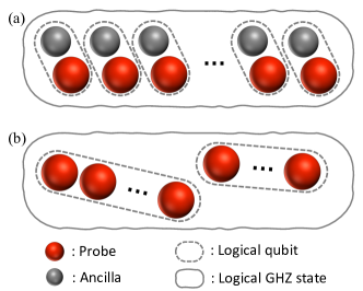
Figure 1: (a) Ancilla-assisted QEC strategy. For example, in Eq. (8), one probe and one noiseless ancilla encode one logical qubit. The HL ($\delta\omega=O(1/N)$) is achieved by preparing a logical GHZ state using $N$ logical qubits. (b) Ancilla-free multi-probe QEC strategy. For example, in Eq. (15), $m=\Theta(N)$ probes encode one logical qubit. The HL is achieved by preparing a logical GHZ state containing $O(1)$ number of logical qubits.

In general, the density operator $\rho$ of each $d$-dimensional probe ($d\geq 2$) evolves according to the master equation Breuer et al. (2002)

$$\frac{d\rho}{dt}=-i[\omega H,\rho]+\sum_{i=1}^{r}L_{i}\rho L_{i}^{\dagger}-\frac{1}{2}\{L_{i}^{\dagger}L_{i},\rho\}.$$ (3)

Here $\omega H$ is the Hamiltonian of the probe and $L_{i}$ are the Lindblad operators that cause dissipation in the system. The noise is assumed to be known and independent of $\omega$. Define ${\mathcal{S}}$ to be the linear subspace of Hermitian operators spanned by ${\mathbbm{1}},L_{i},L_{i}^{\dagger}$ and $L_{i}^{\dagger}L_{j}$ for all $i,j$. The HNLS condition states that the HL is achievable using adaptive quantum strategies Demkowicz-Dobrzański and Maccone (2014) (see also Appx. A) if and only if HNLS holds, i.e., $H\notin{\mathcal{S}}$ Demkowicz-Dobrzański et al. (2017); Zhou et al. (2018). The QEC sensing strategy is a special type of adaptive quantum strategies where the QEC operations act sufficiently fast on the probe and ancilla. When HNLS holds, the HL is achievable using QEC Zhou et al. (2018) and, up to an aribitrarily small error,

$$F(\rho_{\omega}(t))=4N^{2}t^{2}\left\|H-{\mathcal{S}}\right\|^{2}=4N^{2}t^{2}\min_{S\in{\mathcal{S}}}\left\|H-S\right\|^{2},$$ (4)

where $\left\|\cdot\right\|$ is the operator norm. Moreover, the HL coefficient, defined by,

$$\sup_{t>0}\lim_{N\rightarrow\infty}\frac{F(\rho_{\omega}(t))}{N^{2}t^{2}}=4\left\|H-{\mathcal{S}}\right\|^{2},$$ (5)

cannot be surpassed via arbitrary adaptive quantum strategies Wan and Lasenby (2022), indicating the optimality of QEC. When HNLS fails, we must have $F(\rho_{\omega}(t))=O(N)$ and the optimal SQL coefficient $\sup_{t>0}\lim_{N\rightarrow\infty}{F(\rho_{\omega}(t))}/{(Nt)}$ is also achievable using QEC Zhou and Jiang (2020) (see also Appx. F). We will say a QEC code achieves the optimal HL (or SQL) if and only if there is a corresponding QEC strategy that achieves the HL (or SQL) and its optimal coefficient.

Assuming HNLS holds, a QEC code assisted by noiseless ancillas can attain the optimal HL (the SQL case Zhou and Jiang (2020) is elaborated in Appx. F.) As proven in Zhou et al. (2018), there exist two density matrices $\rho_{0}$ and $\rho_{1}$ in the probing system such that $\mathrm{Tr}(\rho_{0}\rho_{1})=0$, and

$$\mathrm{Tr}((\rho_{0}-\rho_{1})H)=2\left\|H-{\mathcal{S}}\right\|,$$ (6)

$$\mathrm{Tr}((\rho_{0}-\rho_{1})S)=0,\;\forall S\in{\mathcal{S}}.$$ (7)

Let $\rho_{0}=\sum_{i=0}^{d_{0}-1}\lambda_{i}\ket{i}_{P}\bra{i}_{P}$ and $\rho_{1}=\sum_{i=d_{0}}^{d-1}\lambda_{i}\ket{i}_{P}\bra{i}_{P}$, where $\{\ket{i}_{P}\}_{i=0}^{d-1}$ is an orthonormal basis of the probe space ${\mathcal{H}}_{P}$ and $\sum_{i=0}^{d_{0}-1}\lambda_{i}=\sum_{i=d_{0}}^{d-1}\lambda_{i}=1$. The ancilla-assisted code Zhou et al. (2018) is defined in ${\mathcal{H}}_{P}\otimes{\mathcal{H}}_{A}$ by

$$\ket{0_{\textsc{l}}}=\!\sum_{i=0}^{d_{0}-1}\!\sqrt{\lambda_{i}}\ket{i}_{P}\!\ket{i}_{A},\;\;\ket{1_{\textsc{l}}}=\!\sum_{i=d_{0}}^{d-1}\!\sqrt{\lambda_{i}}\ket{i}_{P}\!\ket{i}_{A},$$ (8)

where $\{\ket{i}_{A}\}_{i=0}^{d-1}$ is an orthonormal basis of the ancillary system ${\mathcal{H}}_{A}$, assumed to be unaffected by both the signal and the noise. (We consider only two-dimensional codes in this paper because it is sufficient for single-parameter estimation.) Using the ancilla-assisted code, there exists a QEC strategy such that the logical qubit evolves noiselessly as a logical Pauli-Z rotation (up to an arbitrarily small error):

$$\frac{d\rho_{\textsc{l}}}{dt}=-i\left[\omega\left\|H-{\mathcal{S}}\right\|Z_{\textsc{l}},\rho_{\textsc{l}}\right],$$ (9)

where $Z_{\textsc{l}}$ is the logical Pauli-Z operator. The logical GHZ state then achieves the optimal HL (see Fig. 1(a)).

Qutrit Example

Generically, every probe needs to be accompanied by a noiseless ancilla of the same dimension in order to achieve the HL. It is a stringent requirement in practical experiments, but can be relaxed in special cases. For example, consider a qubit evolving under a Pauli-Z Hamiltonian and a bit-flip (Pauli-X) noise Kessler et al. (2014); Dür et al. (2014); Arrad et al. (2014); Ozeri (2013); Peng and Fan (2020), the ancilla-free repetition code that entangles three qubits $\ket{k_{\textsc{l}}}=\ket{k}^{\otimes 3}_{P}$ (for $k=0,1$) performs equally well as the ancilla-assisted code $\ket{k_{\textsc{l}}}=\ket{k}_{P}\ket{k}_{A}$ (for $k=0,1$) in terms of achieving the optimal HL.

In this work, we will see how the number of noiseless ancillas can be dramatically reduced using multi-probe encodings (see Fig. 1(b)). We first illustrate this idea in a qutrit example (see details in Appx. B). Consider the qutrit evolution $\frac{d\rho}{dt}=-i[\omega H,\rho]+L\rho L^{\dagger}-\frac{1}{2}\{L^{\dagger}L,\rho\}$, where $H=\ket{0}\bra{0}-(\ket{1}\bra{1}+\ket{2}\bra{2}+\ket{1}\bra{2}+\ket{2}\bra{1})$ and $L=\ket{0}\bra{1}+\ket{0}\bra{2}+\ket{1}\bra{2}$. HNLS holds and we have $\rho_{0}=\frac{1}{2}(\ket{0}\bra{0}+\ket{2}\bra{2})$, $\rho_{1}=\ket{1}\bra{1}$. The ancilla-assisted code is then

$$\ket{0_{\textsc{l}}}=\frac{1}{\sqrt{2}}(\ket{0}_{P}\ket{0}_{A}+\ket{2}_{P}\ket{2}_{A}),\;\;\ket{1_{\textsc{l}}}=\ket{1}_{P}\ket{1}_{A}.$$ (10)

We call it a $(1,1)$-qutrit code, for the encoding contains $1$ qutrit probe and $1$ qutrit ancilla.

As proven in Appx. B, a $(m,1)$-qutrit code in ${\mathcal{H}}_{P}^{\otimes m}\otimes{\mathcal{H}}_{A}$ achieves the optimal HL if it satisfies, for any $k,k^{\prime}=0,1$, $\ell\neq\ell^{\prime}$ and $\ell,\ell^{\prime}=1,\ldots,m$,

$$\mathrm{Tr}_{\backslash\{\ell,\ell^{\prime}\}}(\ket{k_{\textsc{l}}}\bra{k^{\prime}_{\textsc{l}}})=(\rho_{k}^{(\ell)}\otimes\rho_{k}^{(\ell^{\prime})}-Q_{k}^{(\ell)}\otimes Q_{k}^{(\ell^{\prime})})\delta_{kk^{\prime}},$$ (11)

where $\mathrm{Tr}_{\backslash\{\ell,\ell^{\prime}\}}$ means tracing out the entire system except for the $\ell$-th and $\ell^{\prime}$-th probes, we use ^(ℓ) to denote an operator acting on the $\ell$-th probe and $Q_{k}$ can be any traceless Hermitian operator satisfying $\mathrm{Tr}(Q_{k}L_{i})=0,\forall i$. We call Eq. (11) a multi-probe QEC condition in this paper. For example, the repetition code for Pauli-Z signal and Pauli-X noise satisfies it, i.e., $\mathrm{Tr}_{\backslash\{\ell,\ell^{\prime}\}}(\ket{k}\bra{k^{\prime}}^{\otimes 3})=\rho_{k}^{\otimes 2}\delta_{kk^{\prime}}$ where $\rho_{k}=\ket{k}\bra{k}$ and $Q_{k}=0$. In the qutrit case above, a $(4,1)$-qutrit code satisfying this condition for $m=4$ is

$$\ket{0_{\textsc{l}}}=\frac{1}{\sqrt{6}}\big{(} (\ket{0022}_{P^{\otimes 4}}+\ket{2200}_{P^{\otimes 4}})\ket{0}_{A}$$

$$+ (\ket{0202}_{P^{\otimes 4}}+\ket{2020}_{P^{\otimes 4}})\ket{1}_{A}$$

$$+ (\ket{0220}_{P^{\otimes 4}}+\ket{2002}_{P^{\otimes 4}})\ket{2}_{A}\big{)},$$ (12)

and $\ket{1_{\textsc{l}}}=\ket{1111}_{P^{\otimes 4}}\ket{0}_{A}$.

The advantage of a smaller number of ancillas arises when the noiseless ancilla is a limited resource. Imagine a simplified scenario where a qutrit probe and a qutrit noiseless ancilla are two equivalent units of resource (in reality the latter can be more difficult to prepare, e.g., a noiseless ancilla can be replaced by a constant number of noisy probes under inner QEC Zhou et al. (2018)). Then the achievable QFI using $N_{\textsc{u}}$ units of resource in a probing time $t$ is $\frac{1}{4}N_{\textsc{u}}^{2}t^{2}$ via the $(1,1)$-qutrit encoding and a $\frac{N_{\textsc{u}}}{2}$-qubit logical GHZ state, and $\frac{16}{25}N_{\textsc{u}}^{2}t^{2}$ via the $(4,1)$-qutrit encoding and a $\frac{4N_{\textsc{u}}}{5}$-qubit logical GHZ state. Clearly, a higher sensitivity is achieved when more resources can be used as probes instead of ancillas.

Ancilla-free QEC codes

Here we present two types of QEC codes that achieve the optimal HL when HNLS holds, where the fraction of noiseless ancillas is negligible asymptotically. The QEC codes that achieve the optimal SQL when HNLS fails can be defined analogously, with details provided in Appx. F.

The first code, which we will refer to as small-ancilla code, entangles $m\geq 3$ probes and one ancilla (i.e., ${\mathcal{H}}_{P}^{\otimes m}\otimes{\mathcal{H}}_{A}$). We will prove later that it achieves the optimal HL when $m=\Theta(N)$, although in special circumstances (e.g., the $(4,1)$-qutrit code), the optimal HL is achievable with a constant $m$. The codewords are

$$\ket{k_{\textsc{l}}}=\frac{1}{\sqrt{\left|W_{k}\right|}}\sum_{w\in W_{k}}\ket{w}_{P^{\otimes m}}\ket{{\mathfrak{i}}_{k}(w)}_{A},$$ (13)

for $k=0,1$. Here we use $\ket{w}$ to denote $\ket{w_{1}}\otimes\cdots\otimes\ket{w_{m}}$ for any string $w=w_{1}w_{2}\cdots w_{m}\in\{0,\ldots,d-1\}^{m}$. $W_{0}$ and $W_{1}$ are two non-overlapping sets of strings of length $m$ and $\left|W_{k}\right|$ denotes the order of $W_{k}$. To define $W_{0,1}$, note that for all $m$, it is possible to find a set of integers $\{m_{i}\}_{i=0}^{d-1}$ such that $\sum_{i=0}^{d_{0}-1}m_{i}=\sum_{i=d_{0}}^{d-1}m_{i}=m$ and

$$\left|\frac{m_{i}}{m}-\lambda_{i}\right|\leq\frac{1}{m},\;\forall i=0,\ldots,d-1.$$ (14)

Note that it satisfies $\lim_{m\rightarrow\infty}m_{i}/m=\lambda_{i}$. We then define $W_{0}$ (or $W_{1}$) to be the set of strings that contains $m_{i}$ $i$’s for $0\leq i\leq d_{0}-1$ (or $d_{0}\leq i\leq d-1$).

Note that the above construction guarantees that for $m\gg 1$, $k,k^{\prime}=0,1$ and $\ell\neq\ell^{\prime}$, the multi-probe QEC condition (choosing $Q_{k}=0$) is satisfied approximately, which is a key ingredient in proving the optimality of the small-ancilla code.

The second code exploits random phases such that the multi-probe QEC condition holds when $m\gg 1$. We call it ancilla-free random code, which entangles $m\geq 3$ probes without ancillas (i.e., ${\mathcal{H}}_{P}^{\otimes m}$). It also achieves the optimal HL when $m=\Theta(N)$, and is defined by

$$\ket{k_{\textsc{l}}}=\frac{1}{\sqrt{\left|W_{k}\right|}}\sum_{w\in W_{k}}e^{i\theta_{w}}\ket{w}_{P^{\otimes m}},$$ (15)

for $k=0,1$, where $\{\theta_{w}\}_{w\in W_{0}\cup W_{1}}$ are sampled from a set of independent and identically distributed random variables following the uniform distribution in $[0,2\pi)$. The ancilla-free random code achieves the optimal HL when $m=\Theta(N)$ with probability $1-e^{-\Omega(m)}$.

QEC strategy

Now we delve into the details of the QEC strategy, in particular the recovery channel, and explain how our (effectively) ancilla-free codes achieve the optimal HL. (The SQL case is discussed in Appx. F.) In particular, we will show that there exists a QEC strategy such that the signal strength increases linearly with $N$, while the noise rate at most a constant, leading to the HL.

We first examine the form of logical master equations, i.e., the logical state evolution under QEC, and identify the optimal choice of recovery channels. Let $P=\ket{0_{\textsc{l}}}\bra{0_{\textsc{l}}}+\ket{1_{\textsc{l}}}\bra{1_{\textsc{l}}}$ be the projection operator onto the code subspace. The QEC sensing strategies are performed by constantly applying the quantum channel ${\mathcal{P}}+{\mathcal{R}}\circ{\mathcal{P}}_{\perp}$ on the quantum state Zhou et al. (2018); Zhou and Jiang (2020), where ${\mathcal{P}}(\cdot)=P(\cdot)P$, ${\mathcal{P}}_{\perp}(\cdot)=P_{\perp}(\cdot)P_{\perp}$, $P_{\perp}={\mathbbm{1}}-P$ and ${\mathcal{R}}$ is a recovery channel satisfying ${\mathcal{R}}={\mathcal{P}}\circ{\mathcal{R}}$. Then the multi-probe logical state $\rho_{\textsc{l}}$ (satisfying $\rho_{\textsc{l}}=P\rho_{\textsc{l}}P$) evolves as (see Appx. D)

$$\frac{d\rho_{\textsc{l}}}{dt}=-i\left[\omega{\mathcal{P}}\left(\sum_{\ell=1}^{m}H^{(\ell)}\right),\rho_{\textsc{l}}\right]+\sum_{i=1}^{r}\sum_{\ell=1}^{m}{\mathcal{P}}\left(L_{i}^{(\ell)}\rho_{\textsc{l}}L_{i}^{(\ell)\dagger}\right)\\ +{\mathcal{R}}\left({\mathcal{P}}_{\perp}\left(L_{i}^{(\ell)}\rho_{\textsc{l}}L_{i}^{(\ell)\dagger}\right)\right)-\frac{1}{2}\left\{{\mathcal{P}}\left(L_{i}^{(\ell)\dagger}L_{i}^{(\ell)}\right),\rho_{\textsc{l}}\right\}.$$ (16)

Furthermore, let ${\mathfrak{L}}_{k}={\rm span}\{\ket{k_{\textsc{l}}},L_{i}^{(\ell)}\ket{k_{\textsc{l}}},\forall i,\ell\}$ for $k=0,1$, where ${\rm span}\{\cdot\}$ denotes the linear span of states and assume that (i) ${\mathfrak{L}}_{0}\perp{\mathfrak{L}}_{1}$; (ii) the recovery channel has the form

$${\mathcal{R}}(\cdot)\!=\!\sum_{p}(\ket{0_{\textsc{l}}}\bra{R_{p}}+\ket{1_{\textsc{l}}}\bra{S_{p}})(\cdot)(\ket{R_{p}}\bra{0_{\textsc{l}}}+\ket{S_{p}}\bra{1_{\textsc{l}}}),$$ (17)

where $\{\ket{R_{p}},\ket{S_{p}},\forall p\}$ is an orthonormal basis of ${\mathcal{H}}_{P}^{\otimes m}\otimes{\mathcal{H}}_{A}$, such that ${\mathfrak{L}}_{0}\subseteq{\rm span}\{\ket{R_{p}},\forall p\}$ and ${\mathfrak{L}}_{1}\subseteq{\rm span}\{\ket{S_{p}},\forall p\}$. Then the logical master equation is described by (see Appx. D)

$$\frac{d\rho_{\textsc{l}}}{dt}=-i\left[\frac{\omega\mathrm{Tr}(\sum_{\ell}H^{(\ell)}Z_{\textsc{l}})}{2}Z_{\textsc{l}}+\beta_{\textsc{l}}({\mathcal{R}})Z_{\textsc{l}},\rho_{\textsc{l}}\right]\\ +\frac{\gamma_{\textsc{l}}({\mathcal{R}})}{2}(Z_{\textsc{l}}\rho_{\textsc{l}}Z_{\textsc{l}}-\rho_{\textsc{l}}),$$ (18)

where $\beta_{\textsc{l}}({\mathcal{R}})$ and $\gamma_{\textsc{l}}({\mathcal{R}})$ are functions of ${\mathcal{R}}$. Note that the Hamiltonian term $\beta_{\textsc{l}}({\mathcal{R}})Z_{\textsc{l}}$ can be ignored because it is independent of $\omega$, commutes with the system dynamics, and thus will not contribute to the QFI. We choose the recovery channel (of the form Eq. (17)) that attains the minimum logical noise rate

$$\gamma_{\textsc{l}}:=\min_{\ket{R_{p}},\ket{S_{p}}}\gamma({\mathcal{R}})=\sum_{i=1}^{r}\sum_{\ell=1}^{m}-{\mathrm{Re}}[\bra{0_{\textsc{l}}}L_{i}^{(\ell)}\ket{0_{\textsc{l}}}\bra{1_{\textsc{l}}}L_{i}^{(\ell)\dagger}\ket{1_{\textsc{l}}}]$$

$$+\frac{1}{2}(\bra{0_{\textsc{l}}}L_{i}^{(\ell)\dagger}L_{i}^{(\ell)}\ket{0_{\textsc{l}}}+\bra{1_{\textsc{l}}}L_{i}^{(\ell)\dagger}L_{i}^{(\ell)}\ket{1_{\textsc{l}}})$$ (19)

$$-\left\|\sum_{i=1}^{r}\sum_{\ell=1}^{m}({\mathbbm{1}}-\ket{0_{\textsc{l}}}\bra{0_{\textsc{l}}})(L_{i}^{(\ell)}\ket{0_{\textsc{l}}}\bra{1_{\textsc{l}}}L_{i}^{(\ell)\dagger})({\mathbbm{1}}-\ket{1_{\textsc{l}}}\bra{1_{\textsc{l}}})\right\|_{1},$$

where $\left\|\cdot\right\|_{1}$ is the trace norm.

The discussions above hold for any QEC encoding and recovery that satisfy assumptions (i) and (ii), including the ancilla-assisted code (taking $m=1$), the small-ancilla code, and the ancilla-free random code.

As a sanity check and a preparation for later proofs, we first show that $\gamma_{\textsc{l}}=0$ for the ancilla-assisted code (taking $m=1$), recovering Eq. (9). We first notice that the transformations (i) $L_{i}\leftarrow L_{i}-x_{i}{\mathbbm{1}}$ for any $x_{i}\in{\mathbb{C}}$ and (ii) $L_{i}\leftarrow\sum_{j}u_{ij}L_{j}$ for any isometry $u$ satisfying $\sum_{i}u_{ik}^{*}u_{ij}=\delta_{kj}$ introduces at most an irrelevant parameter-independent Pauli-Z Hamiltonian in Eq. (18). Therefore, without loss of generality, we can always assume (also using Eq. (7)) that

$$\mathrm{Tr}(\rho_{0}L_{i})=\mathrm{Tr}(\rho_{1}L_{i})=0,\;\forall i$$ (20)

$$\mathrm{Tr}(\rho_{0}L_{i}^{\dagger}L_{j})=\mathrm{Tr}(\rho_{1}L_{i}^{\dagger}L_{j})=\mu_{i}\delta_{ij},\;\forall i,j,$$ (21)

where $\mu_{i}\geq 0$. Eq. (8) implies $\braket{0_{\textsc{l}}}{L_{i}}{0_{\textsc{l}}}=\braket{1_{\textsc{l}}}{L_{i}}{1_{\textsc{l}}}=0$ and $\braket{0_{\textsc{l}}}{L_{i}^{\dagger}L_{j}}{0_{\textsc{l}}}=\braket{1_{\textsc{l}}}{L_{i}^{\dagger}L_{j}}{1_{\textsc{l}}}=\mu_{i}\delta_{ij}$, leading to $\gamma_{\textsc{l}}=\sum_{i=1}^{r}\mu_{i}-\big{\|}\sum_{i=1}^{r}L_{i}\ket{0_{\textsc{l}}}\bra{1_{\textsc{l}}}L_{i}^{\dagger}\big{\|}_{1}=0$.

Consider $n$ logical qubits (the total number of probes is $N=mn$), evolving under Eq. (18) with an initial state $\ket{\psi_{\rm in}}=\frac{1}{\sqrt{2}}(\ket{0_{\textsc{l}}}^{\otimes n}+\ket{1_{\textsc{l}}}^{\otimes n})$. We have (from Eq. (2)) that

$$F(\rho_{\omega}(t))=n^{2}\left(\sum_{\ell=1}^{m}\mathrm{Tr}(H^{(\ell)}Z_{\textsc{l}})\right)^{2}t^{2}e^{-2n\gamma_{\textsc{l}}t}.$$ (22)

Taking $m=1$, $n=N$, $\gamma_{\textsc{l}}=0$ and $\mathrm{Tr}(H^{(\ell)}Z_{\textsc{l}})=2\left\|H-{\mathcal{S}}\right\|$, it is obvious that the optimal HL is achieved using the ancilla-assisted code.

For the multi-probe codes, $\gamma_{\textsc{l}}$ is sometimes positive due to the fact that Eq. (11) is only approximately true. Nonetheless, the optimal HL is still achievable, because $\gamma_{\textsc{l}}$ is at most a constant as $N$ increase. (Note that without QEC, the noise rate will increase linearly with respect to $N$.) Specifically, the multi-probe code satisfies

$$F(\rho_{\omega}(t))=n^{2}m^{2}\mathrm{Tr}((\tilde{\rho}_{0}-\tilde{\rho}_{1})H)^{2}t^{2}e^{-2n\gamma_{\textsc{l}}t},$$ (23)

where $\tilde{\rho}_{k}=\mathrm{Tr}_{\backslash\{\ell\}}(\ket{k_{\textsc{l}}}\bra{k_{\textsc{l}}})$ for $k=0,1$, where $\mathrm{Tr}_{\backslash\{\ell\}}$ means tracing out the entire system except for the $\ell$-th probe. (Note that $\tilde{\rho}_{k}=\rho_{k}+O(1/m)$ is independent of $\ell$.) The optimal HL (Eq. (5)) is then achievable, taking $n=\Theta(1)$ and $m=\Theta(N)$, if

$$\lim_{m\rightarrow\infty}\mathrm{Tr}((\tilde{\rho}_{0}-\tilde{\rho}_{1})H)=2\left\|H-{\mathcal{S}}\right\|,$$ (24)

$$\limsup_{m\rightarrow\infty}\gamma_{\textsc{l}}=\overline{\gamma}_{\textsc{l}}<+\infty.$$ (25)

In particular, when $\overline{\gamma}_{\textsc{l}}>0$, the optimal HL is achieved in the regime $t\ll 1/\overline{\gamma}_{\textsc{l}}$. The proofs of Eq. (24) and Eq. (25) are left in Appx. E.

Discussion

This work answers the long-standing open question of the requirement of noiseless ancillas in noisy quantum metrology. To achieve this, we constructed two types of multi-probe QEC codes that are (effectively) ancilla-free and achieve the optimal HL when HNLS holds (or the optimal SQL when HNLS fails). We started from the previously known optimal ancilla-assisted QEC code that entangles one probe and one ancilla and designed multi-probe codes such that their 2-local reduced density operators resemble those of ancilla-assisted codes. We then proved their optimality by choosing suitable recovery channels.

There are several open problems remain to be addressed. First, our ancilla-free codes are only proven optimal when the number of probes are sufficiently large, and the performance of our codes in a small-size quantum sensor might be suboptimal and remains to be investigated. Second, our codes achieve the optimal HL with respect to the number of probes, but sometimes fails when the probing time is too long and it remains open where there are ancilla-free code that achieves the optimal HL with respect to the probing time. Finally, efficient encoding and decoding algorithms are yet to be found for our multi-probe codes.

Appendix A Adaptive quantum strategies and QEC strategies for noisy quantum metrology

In this appendix, we explain in detail the common metrological strategies used in noisy quantum metrology, and clarify our definitions of the HL and the SQL in the main text. We consider Hamiltonian estimation under Markovian noise where the probe evolution is described by Eq. (3). Let the quantum channel

$${\mathcal{E}}_{\omega}(\rho)=\rho+\left(-i[\omega H,\rho]+\sum_{i=1}^{r}L_{i}\rho L_{i}^{\dagger}-\frac{1}{2}\{L_{i}^{\dagger}L_{i},\rho\}\right)dt+O(dt^{2})$$ (26)

describe the probe evolution in a small time $dt$.

Adaptive quantum strategies (or sequential strategies, shown in Fig. S1(a)) are usually considered as the most general quantum strategies Demkowicz-Dobrzański and Maccone (2014); Sekatski et al. (2017); Demkowicz-Dobrzański et al. (2017), where the system consists of a probe and an ancillary system of an arbitrarily large dimension. Arbitrary quantum controls (i.e., quantum channels) ${\mathcal{C}}_{1},{\mathcal{C}}_{2},\ldots$ are applied instantaneously every time interval $dt$. The total number of controls are $T/dt$, where $T$ is the probing time. The goal is to maximize the QFI of final states $\rho_{\omega}$ over all quantum controls and initial states $\ket{\psi_{\rm in}}$, taking the limit $dt\rightarrow 0$. It was shown that Demkowicz-Dobrzański et al. (2017); Zhou et al. (2018); Wan and Lasenby (2022), for any adaptive quantum strategy, we always have

$$F(\rho_{\omega}(T))\leq 4\left\|H-{\mathcal{S}}\right\|T^{2}+O(T),$$ (27)

when HNLS holds (i.e., $H\notin{\mathcal{S}}$). In this case, there exists an ancilla-assisted QEC strategy achieving $F(\rho_{\omega})=\Theta(T^{2})$ Zhou et al. (2018). On the other hand, when HNLS fails (i.e., $H\in{\mathcal{S}}$), we always have

$$F(\rho_{\omega}(T))\leq 4\alpha T,\quad\alpha:=\min_{\begin{subarray}{c}h\in{\mathbb{C}}^{r},\text{\leavevmode\nobreak\ Hermitian\leavevmode\nobreak\ }{\mathfrak{h}}\in{\mathbb{C}}^{r\times r},\text{\leavevmode\nobreak\ s.t.\leavevmode\nobreak\ }\\ H-\sum_{j}(h_{j}^{*}L_{j}+h_{j}L_{j}^{\dagger})-\sum_{ij}{\mathfrak{h}}_{ij}L_{i}^{\dagger}L_{j}\propto{\mathbbm{1}}\end{subarray}}\left\|\sum_{i}\bigg{(}\sum_{j}h_{j}{\mathbbm{1}}+{\mathfrak{h}}_{ij}L_{j}\bigg{)}^{\dagger}\bigg{(}\sum_{j}h_{j}{\mathbbm{1}}+{\mathfrak{h}}_{ij}L_{j}\bigg{)}\right\|.$$ (28)

It means the QFI cannot go beyond the SQL.

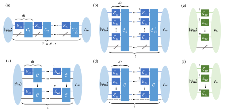
Figure S1: (a)-(d) Hamiltonian estimation under Markovian noise. (a) Adaptive quantum strategies (or sequential strategies). (b) Parallel strategies. (c) Ancilla-assisted QEC strategies. (d) Multi-probe QEC strategies that are effectively ancilla-free. Here we set the number of probes in a logical qubit $m$ equal to the total number of probes $N$; while in general $N$ can be a multiple of $m$ and the QEC operation will act repeatedly in parallel on each multi-probe logical qubit like in (c). Note that we use slashes over lines to represent ancillary systems whose dimension can be arbitrarily large; and dashed lines to denote small ancillary systems whose dimensions are exponentially small compared to the dimension of the probes. (e)-(f) Quantum channel estimation. (e) Parallel strategies. (f) Ancilla-free parallel strategies.

Parallel strategies form a subset of adaptive quantum strategies, as shown in Fig. S1(b), where the system consists of $N$ probes and an ancillary system of an arbitrarily large dimension and the probing time is taken as $t=T/N$ (in comparison to the probing time $T$ in adaptive quantum strategies). Fig. S1(b) can be reduced to Fig. S1(a) if we apply in each step in Fig. S1(a) a swap gate between the probe and one ancilla, making parallel strategies a subset of adaptive strategies. Therefore, we have, for parallel strategies,

$$F(\rho_{\omega}(t))\leq\begin{cases}4\left\|H-{\mathcal{S}}\right\|N^{2}t^{2}+O(Nt),&\text{\leavevmode\nobreak\ when\leavevmode\nobreak\ }H\notin{\mathcal{S}},\\ 4\alpha Nt,&\text{\leavevmode\nobreak\ when\leavevmode\nobreak\ }H\in{\mathcal{S}}.\end{cases}$$ (29)

When we fix $t$ and let $N\rightarrow\infty$, the scaling $F(\rho_{\omega})=\Theta(N^{2})$ is the HL with respect to the number of probes $N$, which is the definition of HL we focus on in this work. In particular, we define the asymptotic HL (or SQL) coefficient to be $\sup_{t>0}\lim_{N\rightarrow\infty}{F(\rho_{\omega}(t))}/{(Nt)^{2}}$ (or $\sup_{t>0}\lim_{N\rightarrow\infty}{F(\rho_{\omega}(t))}/{(Nt)}$) and we say a metrological protocol achieves the optimal asymptotic HL (or SQL) coefficient if the coefficient reaches its upper bound $4\left\|H-{\mathcal{S}}\right\|^{2}$ (or $4\alpha$). On the other hand, when we fix $N$ and let $t\rightarrow\infty$, the scaling $F(\rho_{\omega})=\Theta(t^{2})$ is the HL with respect to the probing time $t$. Our ancilla-free QEC strategies do not necessarily reach the HL with respect to $t$.

We discuss in this work both the case where the HL (with respect to $N$) is achievable and the case where only the SQL (with respect to $N$) is achievable. In particular, we design (effectively) ancilla-free QEC strategies that achieve the optimal HL (or SQL) with respect to $N$, where only the ancilla-assisted QEC procotols were known previously Zhou et al. (2018); Zhou and Jiang (2020).

The QEC metrological strategies are special types of parallel strategies. Fig. S1(c) illustrates the ancilla-assisted QEC strategy, e.g., using the ancilla-assisted code (Eq. (8)) when HNLS holds, or the ancilla-assisted code${}^{\textsc{sql}}$ (Eq. (107)) when HNLS fails, where the QEC operation ${\mathcal{C}}$ applies repeatedly in parallel on each pair of a probe and an ancilla of the same dimension (or twice the probe’s dimension in the SQL case).

Fig. S1(d) illustrates our newly introduced multi-probe QEC strategies that is effectively ancilla-free. For simplicity, Fig. S1(d) specifically shows the case where $m$, the number of probes in a logical qubit, is equal to $N$ (i.e., we encode the logical qubit in the entire system); while in general $N$ can be a multiple of $m$ and the QEC operation will act repeatedly in parallel on each multi-probe logical qubit like in Fig. S1(c). Our multi-probe QEC strategies include QEC using the small-ancilla code (Eq. (13)) and the ancilla-free random code (Eq. (15)) when HNLS holds, and the the small-ancilla code${}^{\textsc{sql}}$ (Eq. (114)) and the qubit-ancilla random code${}^{\textsc{sql}}$ (Eq. (149)) when HNLS fails. We prove that when $m=\Theta(N)$, the optimal HL is achievable using our multi-probe QEC strategies. Moreover, we show that in order to achieve the optimal HL, we only need an ancilla whose dimension is exponentially smaller than that of the probes. It means that these codes are effectively ancilla-free because the ancilla can always be replaced by a negligible amount of probes under inner QEC.

Previous results on the role of ancilla

Finally, we remark on previous results on the role of ancilla in quantum metrology and related fields.

In quantum channel estimation where ${\mathcal{E}}_{\omega}$ is an arbitary quantum channel as a function of $\omega$, it was previously known that the ancilla-assisted parallel quantum strategy (Fig. S1(e)) performs better than the ancilla-free parallel quantum strategy (Fig. S1(f)) Demkowicz-Dobrzański and Maccone (2014). For phase estimation under amplitude damping noise,

$${\mathcal{E}}_{\omega}(\cdot)=(\ket{0}\bra{0}+\sqrt{\eta}\ket{1}\bra{1})e^{i\frac{\omega}{2}Z}(\cdot)e^{-i\frac{\omega}{2}Z}(\ket{0}\bra{0}+\sqrt{\eta}\ket{1}\bra{1})+(1-\eta)\ket{0}\bra{1}e^{i\frac{\omega}{2}Z}(\cdot)e^{-i\frac{\omega}{2}Z}\ket{1}\bra{0},\;0<\eta<1,$$ (30)

the optimal QFI of the ancilla-assisted parallel strategy is $\frac{4N\eta}{1-\eta}$, larger than the optimal QFI of the ancilla-free parallel strategy $\frac{N\eta}{1-\eta}$ Demkowicz-Dobrzański and Maccone (2014). The result seemingly contradicts with our conclusion that ancilla-free strategies performs equally well as ancilla-assisted strategies in the case of Hamiltonian estimation under Markovian noise. The reason could lie in that we allow frequent QEC acting repeatedly in the system evolution (e.g., in Fig. S1(d)), while in quantum channel estimation no controls are allowed during the channel application, but only before and after it (Fig. S1(f)).

Besides single-parameter quantum metrology, ancilla also plays an important role in multi-parameter quantum metrology. In multi-parameter estimation, the incompatibility of optimal measurements for different parameters is a crucial issue and ancilla helps alleviate such incompatibility. For example, in quantum sensing of magnetic field strength and frequency, a maximally entangled state between the probe and ancillary system reaches the optimal sensitivity Yuan (2016); Hou et al. (2021). In the related field of multi-parameter quantum learning, there can be exponential separations between the sample complexity in the sequential ancilla-assisted case and that in the sequential ancilla-free case Chen et al. (2022). It would be intriguing, in future works, to compare the performance of ancilla-free QEC strategies with the ancilla-assisted QEC strategies Górecki et al. (2020) in multi-parameter noisy quantum metrology.

Appendix B $(4,1)$-qutrit code example

In this appendix, we consider a Markovian noise model on a qutrit. We first derive the ancilla-assisted code which entangles one probe qutrit with one ancillary qutrit (Eq. (8)) and show it achieves the optimal HL. Then we show that the size of ancilla can be reduced by presenting a code that entangles four probes with one ancilary qutrits and we call it a $(4,1)$-qutrit code, which is a special case of the general small-ancilla code (Eq. (13)) in the main text. We show the $(4,1)$-qutrit code also achieves the optimal HL using a multi-probe QEC sensing condition (Lemma S1).

Here we consider a qutrit state $\rho$ evolving according to a master equation

$$\frac{d\rho}{dt}=-i[\omega H,\rho]+L\rho L^{\dagger}-\frac{1}{2}\{L^{\dagger}L,\rho\},$$ (31)

where (we use the $(i+1)$-th row/column to represent a basis state $\ket{i}$ ($i=0,1,2$))

$$H=\begin{pmatrix}1&0&0\\ 0&-1&-1\\ 0&-1&-1\\ \end{pmatrix},\quad L=\begin{pmatrix}0&1&1\\ 0&0&1\\ 0&0&0\\ \end{pmatrix}.$$ (32)

The Lindblad span is ${\mathcal{S}}={\rm span}\left\{{\mathbbm{1}},L+L^{\dagger},i(L-L^{\dagger}),L^{\dagger}L\right\}$, where

$$L+L^{\dagger}=\begin{pmatrix}0&1&1\\ 1&0&1\\ 1&1&0\\ \end{pmatrix},\quad i(L-L^{\dagger})=\begin{pmatrix}0&i&i\\ -i&0&i\\ -i&-i&0\\ \end{pmatrix},\quad L^{\dagger}L=\begin{pmatrix}0&0&0\\ 0&1&1\\ 0&1&2\\ \end{pmatrix}.$$ (33)

We first observe that $H\notin{\mathcal{S}}$. Moreover,

$$\left\|H-{\mathcal{S}}\right\|=\left\|H-S\right\|=\frac{1}{2},\text{\leavevmode\nobreak\ \leavevmode\nobreak\ \leavevmode\nobreak\ where\leavevmode\nobreak\ }S=\frac{1}{2}{\mathbbm{1}}-L^{\dagger}L=\text{\leavevmode\nobreak\ and\leavevmode\nobreak\ }H-S=\begin{pmatrix}\frac{1}{2}&0&0\\ 0&-\frac{1}{2}&0\\ 0&0&\frac{1}{2}\\ \end{pmatrix}.$$ (34)

To find $\rho_{0,1}$ satisfying Eq. (6) and Eq. (7), we use the fact that $\rho_{0}$ is supported on the eigenspace correspondings to the maximum eigenvalue of $H-S$ and $\rho_{1}$ is supported on the eigenspace correspondings to the minimum eigenvalue of $H-S$. Then the only solutions to $\rho_{0}$ and $\rho_{1}$ satisfying Eq. (7) are

$$\rho_{0}=\frac{1}{2}\left(\ket{0}\bra{0}+\ket{2}\bra{2}\right),\quad\rho_{1}=\ket{1}\bra{1}.$$ (35)

Then the ancilla-assisted code is given by

$$\ket{0_{\textsc{l}}}=\frac{1}{\sqrt{2}}(\ket{0}_{P}\ket{0}_{A}+\ket{2}_{P}\ket{2}_{A}),\;\;\ket{1_{\textsc{l}}}=\ket{1}_{P}\ket{1}_{A},$$ (36)

whose reduced density operators in ${\mathcal{H}}_{P}$ are $\rho_{0,1}$. We call it a $(1,1)$-qutrit code, for the encoding contains $1$ qutrit probe and $1$ qutrit ancilla. There exists a recovery channel such that the logical state evolves as Zhou et al. (2018)

$$\frac{d\rho_{\textsc{l}}}{dt}=-i\left[\frac{\omega}{2}Z_{\textsc{l}},\rho_{\textsc{l}}\right].$$ (37)

Before we present the $(4,1)$-qutrit code, we first prove a useful lemma for general QEC sensing that provides a sufficient condition for a code to achieve the optimal HL. Note that it is not a necessary condition for multi-probe QEC sensing to achieve the HL (for example, we can replace $Q_{k}$ with $iQ_{k}$ below, or introduce more than one $Q_{k}$ and sums up all $Q_{k}\otimes Q_{k}$ terms, and the lemma still holds), but in this paper all our constructed codes follow this sufficient condition (at least approximately). Thus, we will focus on it here for simplicity.

Lemma S1 (Multi-probe QEC sensing).

If a two-dimensional QEC code in ${\mathcal{H}}_{P}^{\otimes m}\otimes{\mathcal{H}}_{A}$ ($m\geq 2$) satisfies for $k,k^{\prime}=0,1$, $\ell\neq\ell^{\prime}$ and $\ell,\ell^{\prime}=1,\ldots,m$,

$$\mathrm{Tr}_{\backslash\{\ell,\ell^{\prime}\}}(\ket{k_{\textsc{l}}}\bra{k^{\prime}_{\textsc{l}}})=\left(\rho_{k}^{(\ell)}\otimes\rho_{k}^{(\ell^{\prime})}-Q_{k}^{(\ell)}\otimes Q_{k}^{(\ell^{\prime})}\right)\delta_{kk^{\prime}},$$ (38)

where $\mathrm{Tr}_{\backslash\{\ell,\ell^{\prime}\}}$ means tracing out the entire system except for the $\ell$-th and $\ell^{\prime}$-th probes and $Q_{k}$ can be any traceless Hermitian operator satisfying $\mathrm{Tr}(Q_{k}L_{i})=0,\forall i$, then there exists a QEC strategy such that a logical state $\rho_{\textsc{l}}$ evolves as (up to an arbitrarily small error)

$$\frac{d\rho_{\textsc{l}}}{dt}=-i\left[\omega m\left\|H-{\mathcal{S}}\right\|Z_{\textsc{l}},\rho_{\textsc{l}}\right].$$ (39)

Proof.

We will use a result from Zhou et al. (2018), which states that if for a two-dimensional QEC code in ${\mathcal{H}}_{P}\otimes{\mathcal{H}}_{A}$, the QEC condition

$$\braket{0_{\textsc{l}}}{S}{0_{\textsc{l}}}=\braket{1_{\textsc{l}}}{S}{1_{\textsc{l}}},\quad\braket{0_{\textsc{l}}}{S}{1_{\textsc{l}}}=0,\quad\forall S\in{\mathcal{S}}={\rm span}\{{\mathbbm{1}},L_{i}^{\dagger},L_{i},L_{i}^{\dagger}L_{j},\;\forall i,j\},$$ (40)

is satisfied, then there exists a QEC strategy such that a logical state $\rho_{\textsc{l}}$ evolves as (up to an arbitrarily small error)

$$\frac{d\rho_{\textsc{l}}}{dt}=-i\left[\omega\frac{\braket{0_{\textsc{l}}}{H}{0_{\textsc{l}}}-\braket{1_{\textsc{l}}}{H}{1_{\textsc{l}}}}{2}Z_{\textsc{l}},\rho_{\textsc{l}}\right].$$ (41)

In the multi-probe case, we only need to replace ${\mathcal{S}}$ with a multi-probe Lindblad span ${\mathcal{S}}_{m}$, where

$${\mathcal{S}}_{m}={\rm span}\{{\mathbbm{1}},L_{i}^{\dagger(\ell)},L_{i}^{(\ell)},L_{i}^{\dagger(\ell)}L_{j}^{(\ell^{\prime})},\;\forall i,j,\ell,\ell^{\prime}\},$$ (42)

and the single-probe Hamiltonian $H$ with the multi-probe Hamiltonian $\sum_{\ell=1}^{m}H^{(\ell)}$. Noting that ${\mathcal{S}}_{m}$ contains at most $2$-local operators, i.e., operators that act as identity on all but two probes, and using Eq. (38) and

$$\mathrm{Tr}((Q_{0}\otimes Q_{0})S_{2})=\mathrm{Tr}((Q_{1}\otimes Q_{1})S_{2})=0,\quad\forall S_{2}\in{\mathcal{S}}_{2}={\rm span}\{S\otimes{\mathbbm{1}},{\mathbbm{1}}\otimes S,L_{i}^{\dagger}\otimes L_{j},\forall i,j,S\in{\mathcal{S}}\}$$ (43)

from the definition of $Q_{k}$, the multi-probe QEC condition translates to

$$\mathrm{Tr}((\rho_{0}\otimes\rho_{0})S_{2})=\mathrm{Tr}((\rho_{1}\otimes\rho_{1})S_{2}),\quad\forall S_{2}\in{\mathcal{S}}_{2}={\rm span}\{S\otimes{\mathbbm{1}},{\mathbbm{1}}\otimes S,L_{i}^{\dagger}\otimes L_{j},\forall i,j,S\in{\mathcal{S}}\}.$$ (44)

The above equation holds true because for all $S\in{\mathcal{S}}$,

$$\mathrm{Tr}((\rho_{0}\otimes\rho_{0}-\rho_{1}\otimes\rho_{1})(S\otimes{\mathbbm{1}}))=\mathrm{Tr}((\rho_{0}\otimes\rho_{0}-\rho_{1}\otimes\rho_{1})({\mathbbm{1}}\otimes S))=\mathrm{Tr}((\rho_{0}-\rho_{1})S)=0,$$ (45)

and for all $i,j$,

$$\mathrm{Tr}((\rho_{0}\otimes\rho_{0}-\rho_{1}\otimes\rho_{1})(L_{i}^{\dagger}\otimes L_{j}))=\frac{1}{2}\mathrm{Tr}(((\rho_{0}+\rho_{1})\otimes(\rho_{0}-\rho_{1})+(\rho_{0}-\rho_{1})\otimes(\rho_{0}+\rho_{1}))(L_{i}^{\dagger}\otimes L_{j}))=0.$$ (46)

Finally, we have Eq. (39), noticing that

$$\frac{1}{2}\left(\braket{0_{\textsc{l}}}{\sum_{\ell=1}^{m}H^{(\ell)}}{0_{\textsc{l}}}-\braket{1_{\textsc{l}}}{\sum_{\ell=1}^{m}H^{(\ell)}}{1_{\textsc{l}}}\right)=\frac{1}{2}m\mathrm{Tr}((\rho_{0}-\rho_{1})H)=m\left\|H-{\mathcal{S}}\right\|.$$ (47)

∎

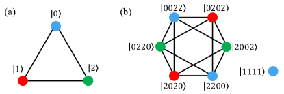
Figure S2: Dimension of ancilla. (a) The dimension of ancilla in the $(1,1)$-qutrit code is $3$. Here we draw a graph where each vertex represents the probe state $\{\ket{0},\ket{1},\ket{2}\}$ and there is an edge between two different states $\ket{w}$ and $\ket{w^{\prime}}$ if and only if there exists $S\in{\mathcal{S}}$ such that $\braket{w}{S}{w^{\prime}}\neq 0$. We use the color of vertices to represent the (orthonormal) basis of the ancilla. We require adjacent vertices to have different colors which is a sufficient condition for QEC. Then at least $3$ colors are required. (b) The dimension of ancilla in the $(4,1)$-qutrit code is $3$. Here we draw a graph where each vertex represents the probe state $\{\ket{0022},\ldots,\ket{1111}\}$ (where $\ldots$ includes all permutations of $\ket{0022}$) and there is an edge between two different states $\ket{w}$ and $\ket{w^{\prime}}$ if and only if there exists $S_{2}\in{\mathcal{S}}_{2}$ and $\ell\neq\ell^{\prime}$ such that $\braket{w}{S_{2}^{(\ell,\ell^{\prime})}}{w^{\prime}}\neq 0$, where $S_{2}^{(\ell,\ell^{\prime})}$ means $S_{2}$ acting on the $\ell$-th and $\ell^{\prime}$-th probes (or equivalently, if and only if $w$ can be obtained from $w^{\prime}$ by swapping two sites with different states). We require adjacent vertices to have different colors which is a sufficient condition for QEC. Then at least $3$ colors are required.

We aim at finding a multi-probe QEC code in ${\mathcal{H}}_{P}^{\otimes m}\otimes{\mathcal{H}}_{A}$ that satisfies the sufficient condition in Lemma S1. Assume $m=4$. Since $\rho_{1}$ is a rank-one operator, we can define

$$\ket{1_{\textsc{l}}}=\ket{1111}_{P^{\otimes 4}}\ket{0}_{A},$$ (48)

which satisfies $\mathrm{Tr}_{\backslash\{\ell,\ell^{\prime}\}}(\ket{1_{\textsc{l}}}\bra{1_{\textsc{l}}})=\rho_{1}\otimes\rho_{1}$ (and $Q_{1}=0$). On the other hand, we define

$$\ket{0_{\textsc{l}}}=\frac{1}{\sqrt{6}}\big{(}(\ket{0022}_{P^{\otimes 4}}+\ket{2200}_{P^{\otimes 4}})\ket{0}_{A}+(\ket{0202}_{P^{\otimes 4}}+\ket{2020}_{P^{\otimes 4}})\ket{1}_{A}+(\ket{0220}_{P^{\otimes 4}}+\ket{2002}_{P^{\otimes 4}})\ket{2}_{A}\big{)},$$ (49)

where the number of appearances of $\ket{0}$ and $\ket{2}$ are tuned so that $\mathrm{Tr}_{\backslash\{\ell,\ell^{\prime}\}}(\ket{0_{\textsc{l}}}\bra{0_{\textsc{l}}})=\rho_{0}\otimes\rho_{0}-Q_{0}\otimes Q_{0}$ and $Q_{0}=\frac{1}{\sqrt{12}}(\ket{0}\bra{0}-\ket{2}\bra{2})$. Note that we also use additional ancillas so that $\mathrm{Tr}_{\backslash\{\ell,\ell^{\prime}\}}(\ket{0_{\textsc{l}}}\bra{0_{\textsc{l}}})$ contains no non-diagonal terms $\ket{02}\bra{20}$ and $\ket{20}\bra{02}$. The minimum dimension of ancillas required is $3$, as illustrated in Fig. S2. Finally, we have $\mathrm{Tr}_{\backslash\{\ell,\ell^{\prime}\}}(\ket{0_{\textsc{l}}}\bra{1_{\textsc{l}}})=0$ because $\ket{1}$ is perpendicular to ${\rm span}\{\ket{0},\ket{2}\}$. Therefore, Eq. (38) is satisfied by the $(4,1)$-qutrit code. Using Lemma S1, we obtain the logical dynamics

$$\frac{d\rho_{\textsc{l}}}{dt}=-i\left[\frac{\omega m}{2}Z_{\textsc{l}},\rho_{\textsc{l}}\right].$$ (50)

The performance of the $(1,1)$-qutrit code and the $(4,1)$-qutrit code are equally optimal in the following sense: if we have $N$ probes that evolves for a probing time $t$, then the QEC strategy using both encodings (where arbitrary numbers of noiseless ancillas are allowed) can prepare a quantum state $\rho_{\omega}(t)$ that has QFI (up to an arbitrarily small error)

$$F(\rho_{\omega}(t))=4\left\|H-{\mathcal{S}}\right\|^{2}N^{2}t^{2}=N^{2}t^{2}.$$ (51)

In practice, however, the $(4,1)$-qutrit code is superior to the $(1,1)$-qutrit code when the noiseless ancilla is not considered as a free resource, which is true because it is must be built of exceedingly stable qubits or noisy qubits under inner QEC. In order to see the advantage of the $(4,1)$-qutrit code, consider the following overly-simplified but illustrative way of resource counting: a qutrit probe and a qutrit noiseless ancilla are considered as two equivalent units of resource and other resources (e.g., QEC operations) are considered free. Then using the $(1,1)$-qutrit code, the achievable QFI using $N_{\textsc{u}}$ units of resource in time $t$ is (assuming $N_{\textsc{u}}$ is a multiple of $2$)

$$F(\rho_{\omega}(t))=\frac{1}{4}N_{\textsc{u}}^{2}t^{2},$$ (52)

and the optimal initial state is

$$\ket{\psi_{\rm in}}=\frac{1}{\sqrt{2}}\left(\ket{0_{\textsc{l}}}^{\otimes N_{\textsc{u}}/2}+\ket{1_{\textsc{l}}}^{\otimes N_{\textsc{u}}/2}\right).$$ (53)

On the other hand, using the $(4,1)$-qutrit code, the achievable QFI using $N_{\textsc{u}}$ units of resource in time $t$ is (assuming $N_{\textsc{u}}$ is a multiple of $5$)

$$F(\rho_{\omega}(t))=\frac{16}{25}N_{\textsc{u}}^{2}t^{2},$$ (54)

and the optimal initial state is

$$\ket{\psi_{\rm in}}=\frac{1}{\sqrt{2}}\left(\ket{0_{\textsc{l}}}^{\otimes 4N_{\textsc{u}}/5}+\ket{1_{\textsc{l}}}^{\otimes 4N_{\textsc{u}}/5}\right).$$ (55)

Clearly, the smaller the ratio between the number of noiseless ancillary qutrits and the number of probe qutrits is, the larger QFI of the final state is. The reason is the QFI is a function of the number of probes only and the more probes there are, the larger the QFI will be. In the case where noiseless ancillas and probes are equivalent units of resource, the QFI of ancilla-free strategy is at most 4 times the QFI of ancilla-assisted strategy; while in practice when noiseless ancillas are more expensive than probes, the advantage of ancilla-free strategies will be even more significant.

Appendix C Upper bound on the dimension of ancilla in small-ancilla codes

Here we count $\dim({\mathcal{H}}_{A})=\left|{\mathfrak{I}}\right|$, the dimension of the noiseless ancilla required for the small-ancilla code (Eq. (13)). The set ${\mathfrak{I}}=\{{\mathfrak{i}}_{k}(w),\forall k=0,1,w\in W_{0}\cup W_{1}\}$ should be large enough such that ${\mathfrak{i}}_{k}(w)$ (for $k=0,1$) can be chosen to be any integer functions that satisfy ${\mathfrak{i}}_{k}(w)\neq{\mathfrak{i}}_{k}(w^{\prime})$ when $w$ and $w^{\prime}$ are different on exactly two sites. Calculating the minimum number of values of ${\mathfrak{i}}_{0}(w)$ required so that ${\mathfrak{i}}_{0}(w)\neq{\mathfrak{i}}_{0}(w^{\prime})$ when $w$ and $w^{\prime}$ are different on exactly two sites is essentially a graph coloring problem (see a qutrit example in Fig. S2(b)), where the elements of $W_{0}$ are vertices of the graph, and there is an edge between $w$ and $w^{\prime}$ as long as $w^{\prime}$ can be obtained from $w$ by swapping two sites with different numbers. We want to know the minimum number of colors required to color the vertices of the graph such that every two adjacent vertices have different colors. Note that the graph is regular—every vertex has the same degree (the number of vertices adjacent to it), which we denote by $\deg(W_{0})$. Similar statements also hold for ${\mathfrak{i}}_{1}(w)$. Then, the minimum value of $\dim({\mathcal{H}}_{A})=\left|{\mathfrak{I}}\right|$ required is at most $\max\{\deg(W_{0})+1,\deg(W_{1})+1\}$, from the Brook’s theorem Brooks (1941). For $k=0$, we have

$$\deg(W_{0})+1=\sum_{i\neq j\leq d_{0}-1}m_{i}m_{j}+1\leq d^{2}m^{2},$$ (56)

and similarly,

$$\deg(W_{1})+1=\sum_{i\neq j\geq d_{0}}m_{i}m_{j}+1\leq d^{2}m^{2}.$$ (57)

Therefore we only need an exponentially small ancilla

$$\dim({\mathcal{H}}_{A})\leq d^{2}m^{2}=o(d^{m}),$$ (58)

compared to the system of $m$ probes.

Appendix D Logical master equations

Consider a logical quantum state $\rho_{\textsc{l}}$ that contains $m$ probes satisfying $\rho_{\textsc{l}}=P\rho_{\textsc{l}}P$ at time $t$. Without QEC, the quantum state at time $t+dt$ satisfies

$$\rho_{\textsc{l}}+d\rho_{\textsc{l}}=\rho_{\textsc{l}}+\left(-i\left[\omega\sum_{\ell=1}^{m}H^{(\ell)},\rho_{\textsc{l}}\right]+\sum_{i=1}^{r}\sum_{\ell=1}^{m}L_{i}^{(\ell)}\rho_{\textsc{l}}L_{i}^{(\ell)\dagger}-\frac{1}{2}\left\{L_{i}^{(\ell)\dagger}L_{i}^{(\ell)},\rho_{\textsc{l}}\right\}\right)dt+O(dt^{2}).$$ (59)

If we apply the QEC operation ${\mathcal{P}}+{\mathcal{R}}\circ{\mathcal{P}}_{\perp}$ on $\rho_{\textsc{l}}$ instantaneously at time $t+dt$, we have

$$\rho_{\textsc{l}}+d\rho_{\textsc{l}}=\rho_{\textsc{l}}+({\mathcal{P}}+{\mathcal{R}}\circ{\mathcal{P}}_{\perp})\Bigg{(}-i\left[\omega\sum_{\ell=1}^{m}H^{(\ell)},\rho_{\textsc{l}}\right]+\sum_{i=1}^{r}\sum_{\ell=1}^{m}L_{i}^{(\ell)}\rho_{\textsc{l}}L_{i}^{(\ell)\dagger}-\frac{1}{2}\left\{L_{i}^{(\ell)\dagger}L_{i}^{(\ell)},\rho_{\textsc{l}}\right\}\Bigg{)}dt+O(dt^{2}).$$ (60)

In the limit of infinitely fast QEC (i.e., $dt\rightarrow 0$), we derive Eq. (16):

$$\frac{d\rho_{\textsc{l}}}{dt}=-i\left[\omega{\mathcal{P}}\left(\sum_{\ell=1}^{m}H^{(\ell)}\right),\rho_{\textsc{l}}\right]+\sum_{i=1}^{r}\sum_{\ell=1}^{m}{\mathcal{P}}\left(L_{i}^{(\ell)}\rho_{\textsc{l}}L_{i}^{(\ell)\dagger}\right)+{\mathcal{R}}\left({\mathcal{P}}_{\perp}\left(L_{i}^{(\ell)}\rho_{\textsc{l}}L_{i}^{(\ell)\dagger}\right)\right)-\frac{1}{2}\left\{{\mathcal{P}}\left(L_{i}^{(\ell)\dagger}L_{i}^{(\ell)}\right),\rho_{\textsc{l}}\right\}.$$ (61)

Note that ${\mathcal{P}}\circ{\mathcal{R}}={\mathcal{R}}$ guarantees that the quantum state always stays in the logical space. Furthermore, we assume ${\mathfrak{L}}_{0}\perp{\mathfrak{L}}_{1}$, where ${\mathfrak{L}}_{k}={\rm span}\{\ket{k_{\textsc{l}}},L_{i}^{(\ell)}\ket{k_{\textsc{l}}},\forall i,\ell\}$ for $k=0,1$, and the recovery channel

$${\mathcal{R}}(\cdot)=\sum_{p}(\ket{0_{\textsc{l}}}\bra{R_{p}}+\ket{1_{\textsc{l}}}\bra{S_{p}})(\cdot)(\ket{R_{p}}\bra{0_{\textsc{l}}}+\ket{S_{p}}\bra{1_{\textsc{l}}}),$$ (62)

where $\{\ket{R_{p}},\ket{S_{p}},\forall p\}$ is an orthonormal basis of ${\mathcal{H}}_{P}^{\otimes m}\otimes{\mathcal{H}}_{A}$, such that ${\mathfrak{L}}_{0}\subseteq{\rm span}\{\ket{R_{p}},\forall p\}$ and ${\mathfrak{L}}_{1}\subseteq{\rm span}\{\ket{S_{p}},\forall p\}$. Then by considering the input and output of the basis of one logical qubit operators $\{\ket{0_{\textsc{l}}}\bra{0_{\textsc{l}}},\ket{0_{\textsc{l}}}\bra{1_{\textsc{l}}},\ket{1_{\textsc{l}}}\bra{0_{\textsc{l}}},\ket{1_{\textsc{l}}}\bra{1_{\textsc{l}}}\}$, we can see that the logical dynamic is described by a dephasing noise and a Pauli-Z rotation, that is, for any $\rho_{\textsc{l}}=P\rho_{\textsc{l}}P$,

$$\frac{d\rho_{\textsc{l}}}{dt}=-i\left[\frac{\omega\mathrm{Tr}(\sum_{\ell}H^{(\ell)}Z_{\textsc{l}})}{2}+\beta_{\textsc{l}}({\mathcal{R}})Z_{\textsc{l}},\rho_{\textsc{l}}\right]+\frac{\gamma_{\textsc{l}}({\mathcal{R}})}{2}(Z_{\textsc{l}}\rho_{\textsc{l}}Z_{\textsc{l}}-\rho_{\textsc{l}}),$$ (63)

where $Z_{\textsc{l}}=\ket{0_{\textsc{l}}}\bra{0_{\textsc{l}}}-\ket{1_{\textsc{l}}}\bra{1_{\textsc{l}}}$,

$$\gamma_{\textsc{l}}({\mathcal{R}})=-\frac{1}{2}(x+x^{*}),\quad\beta_{\textsc{l}}({\mathcal{R}})=-\frac{1}{2i}(x-x^{*}),$$ (64)

and

$$x=\sum_{i=1}^{r}\sum_{\ell=1}^{m}\bra{0_{\textsc{l}}}L_{i}^{(\ell)}\ket{0_{\textsc{l}}}\bra{1_{\textsc{l}}}L_{i}^{(\ell)\dagger}\ket{1_{\textsc{l}}}-\frac{1}{2}(\bra{0_{\textsc{l}}}L_{i}^{(\ell)\dagger}L_{i}^{(\ell)}\ket{0_{\textsc{l}}}+\bra{1_{\textsc{l}}}L_{i}^{(\ell)\dagger}L_{i}^{(\ell)}\ket{1_{\textsc{l}}})\\ +\sum_{p}\bra{R_{p}}({\mathbbm{1}}-\ket{0_{\textsc{l}}}\bra{0_{\textsc{l}}})(L_{i}^{(\ell)}\ket{0_{\textsc{l}}}\bra{1_{\textsc{l}}}L_{i}^{(\ell)\dagger})({\mathbbm{1}}-\ket{1_{\textsc{l}}}\bra{1_{\textsc{l}}})\ket{S_{p}}.$$ (65)

In particular, we are going to pick the optimal ${\mathcal{R}}$ of the form Eq. (17) such that $\gamma_{\textsc{l}}({\mathcal{R}})$ is minimized, and we define

$$\gamma_{\textsc{l}}:=\min_{\ket{R_{p}},\ket{S_{p}}}\gamma_{\textsc{l}}({\mathcal{R}})=\sum_{i=1}^{r}\sum_{\ell=1}^{m}-{\mathrm{Re}}[\bra{0_{\textsc{l}}}L_{i}^{(\ell)}\ket{0_{\textsc{l}}}\bra{1_{\textsc{l}}}L_{i}^{(\ell)\dagger}\ket{1_{\textsc{l}}}]+\frac{1}{2}(\bra{0_{\textsc{l}}}L_{i}^{(\ell)\dagger}L_{i}^{(\ell)}\ket{0_{\textsc{l}}}+\bra{1_{\textsc{l}}}L_{i}^{(\ell)\dagger}L_{i}^{(\ell)}\ket{1_{\textsc{l}}})\\ -\left\|\sum_{i=1}^{r}\sum_{\ell=1}^{m}({\mathbbm{1}}-\ket{0_{\textsc{l}}}\bra{0_{\textsc{l}}})(L_{i}^{(\ell)}\ket{0_{\textsc{l}}}\bra{1_{\textsc{l}}}L_{i}^{(\ell)\dagger})({\mathbbm{1}}-\ket{1_{\textsc{l}}}\bra{1_{\textsc{l}}})\right\|_{1},$$ (66)

where we use $\max_{U:U^{\dagger}U=I}{\mathrm{Re}}[\mathrm{Tr}(BU)]=\left\|B\right\|_{1}$ for any $B$ whose number of columns are no smaller than number of rows.

Appendix E Proof of Eq. (24) and Eq. (25)

To prove Eq. (24) and Eq. (25) for each code, we note first that for both codes,

$$\lim_{m\rightarrow\infty}\tilde{\rho}_{0}=\sum_{i=0}^{d_{0}-1}\lim_{m\rightarrow\infty}\frac{m_{i}}{m}\ket{i}_{P}\bra{i}_{P}=\rho_{0},$$ (67)

$$\lim_{m\rightarrow\infty}\tilde{\rho}_{1}=\sum_{i=d_{0}}^{d-1}\lim_{m\rightarrow\infty}\frac{m_{i}}{m}\ket{i}_{P}\bra{i}_{P}=\rho_{1}.$$ (68)

Then Eq. (24) is proven, using Eq. (6).

We now briefly sketch the proof of Eq. (25) and provide the details later. (Note that we will need to use the fact that, for both codes, ${\mathfrak{L}}_{0}\perp{\mathfrak{L}}_{1}$, where ${\mathfrak{L}}_{k}={\rm span}\{\ket{k_{\textsc{l}}},L_{i}^{(\ell)}\ket{k_{\textsc{l}}},\forall i,\ell\}$ for $k=0,1$.) Using the gauge constraints (Eq. (20) and Eq. (21)), we have

$$\gamma_{\textsc{l}}=m\bigg{(}\sum_{i=1}^{r}{\mu}_{i}-{\mathrm{Re}}[b_{0,i}^{*}b_{1,i}]+\frac{1}{2}(a_{0,ii}+a_{1,ii})\bigg{)}-\left\|B\right\|_{1},$$ (69)

where $b_{k,i}=\braket{k_{\textsc{l}}}{L_{i}^{(\ell)}}{k_{\textsc{l}}}$, $a_{k,ij}=\braket{k_{\textsc{l}}}{L_{i}^{(\ell)\dagger}L_{j}^{(\ell)}}{k_{\textsc{l}}}-\mu_{ij}\delta_{ij}$ for all $k=0,1$, $i,j=1,\ldots,r$, and

$$B=\sum_{i=1}^{r}\sum_{\ell=1}^{m}(L_{i}^{(\ell)}-b_{0,i})\ket{0_{\textsc{l}}}\bra{1_{\textsc{l}}}(L_{i}^{(\ell)}-b_{1,i})^{\dagger}.$$ (70)

The 2nd and 3rd terms in Eq. (69) contribute to $O(1)$ in $\gamma_{\textsc{l}}$ because $b_{k,i}$ and $a_{k,ij}$ are $O(1/m)$ from Eq. (14). To analyze the 4th term $\left\|B\right\|_{1}$, we find two sets of orthonormal states $\{\ket{e_{i,\ell}}\}$ and $\{\ket{f_{i,\ell}}\}$ from $\{(L_{i}^{(\ell)}-b_{0,i})\ket{0_{\textsc{l}}}\}$ and $\{(L_{i}^{(\ell)}-b_{1,i})\ket{1_{\textsc{l}}}\}$ using the Gram–Schmidt procedure. Using $\left\|B\right\|_{1}\geq\left|\sum_{i=1}^{r}\sum_{\ell=1}^{m}\braket{e_{i,\ell}}{B}{f_{i,\ell}}\right|$, we have, for the small-ancilla code, $\left\|B\right\|_{1}\geq m\sum_{i=1}^{r}{\mu}_{i}-O(1)$, implying $\gamma_{\textsc{l}}=O(1)$; and for the ancilla-free random code, the inequality holds true with probability $1-e^{-\Omega(m)}$.

E.1 Proof of Eq. (25) for the small-ancilla code

The small-ancilla code (Eq. (13)) is symmetric (i.e., permutation-invariant) in the probe system. For all $\ell$ and $\ell^{\prime}\neq\ell$, we have

$$b_{0,i} :=\braket{0_{\textsc{l}}}{L_{i}^{(\ell)}}{0_{\textsc{l}}}=\mathrm{Tr}\left(\sum_{i=0}^{d_{0}-1}\left(\frac{m_{i}}{m}-\lambda_{i}\right)\ket{i}\bra{i}\cdot L_{i}\right)=O\left(\frac{1}{m}\right),$$ (71)

$$b_{1,i} :=\braket{1_{\textsc{l}}}{L_{i}^{(\ell)}}{1_{\textsc{l}}}=\mathrm{Tr}\left(\sum_{i=d_{0}}^{d-1}\left(\frac{m_{i}}{m}-\lambda_{i}\right)\ket{i}\bra{i}\cdot L_{i}\right)=O\left(\frac{1}{m}\right),$$ (72)

$$a_{0,ij} :=\braket{0_{\textsc{l}}}{L_{i}^{(\ell)\dagger}L_{j}^{(\ell)}}{0_{\textsc{l}}}-\mu_{i}\delta_{ij}=\mathrm{Tr}\left(\sum_{i=0}^{d_{0}-1}\left(\frac{m_{i}}{m}-\lambda_{i}\right)\ket{i}\bra{i}\cdot L_{i}^{\dagger}L_{j}\right)=O\left(\frac{1}{m}\right),$$ (73)

$$a_{1,ij} :=\braket{1_{\textsc{l}}}{L_{i}^{(\ell)\dagger}L_{j}^{(\ell)}}{1_{\textsc{l}}}-\mu_{i}\delta_{ij}=\mathrm{Tr}\left(\sum_{i=d_{0}}^{d-1}\left(\frac{m_{i}}{m}-\lambda_{i}\right)\ket{i}\bra{i}\cdot L_{i}^{\dagger}L_{j}\right)=O\left(\frac{1}{m}\right),$$ (74)

$$\eta_{0,ij} :=\braket{0_{\textsc{l}}}{L_{i}^{(\ell)\dagger}L_{j}^{(\ell^{\prime})}}{0_{\textsc{l}}}=\frac{mb_{0,i}^{*}b_{0,j}}{m-1}-\sum_{k=0}^{d_{0}-1}\frac{m_{k}}{m(m-1)}\bra{k}L_{i}^{\dagger}\ket{k}\bra{k}L_{j}\ket{k}=O\left(\frac{1}{m}\right),$$ (75)

$$\eta_{1,ij} :=\braket{1_{\textsc{l}}}{L_{i}^{(\ell)\dagger}L_{j}^{(\ell^{\prime})}}{1_{\textsc{l}}}=\frac{mb_{1,i}^{*}b_{1,j}}{m-1}-\sum_{k=d_{0}}^{d-1}\frac{m_{k}}{m(m-1)}\bra{k}L_{i}^{\dagger}\ket{k}\bra{k}L_{j}\ket{k}=O\left(\frac{1}{m}\right).$$ (76)

To derive the equations above, we use the gauge constraints (Eq. (20) and Eq. (21)) and the fact that (we will omit the subscript _P denoting the probe systems in this appendix)

$$\mathrm{Tr}_{\backslash\{\ell,\ell^{\prime}\}}(\ket{0_{\textsc{l}}}\bra{0_{\textsc{l}}})=\sum_{i,j=0}^{d_{0}-1}m_{ij}\ket{ij}\bra{ij},\quad\mathrm{Tr}_{\backslash\{\ell,\ell^{\prime}\}}(\ket{1_{\textsc{l}}}\bra{1_{\textsc{l}}})=\sum_{i,j=d_{0}}^{d-1}m_{ij}\ket{ij}\bra{ij},$$ (77)

where

$$m_{ij}=\frac{1}{m(m-1)}\times\begin{cases}m_{i}m_{j},&i\neq j,\\ m_{i}(m_{i}-1),&i=j.\end{cases}$$ (78)

In particular, it implies

$$\tilde{\rho}_{0}=\mathrm{Tr}_{\backslash\{\ell\}}(\ket{0_{\textsc{l}}}\bra{0_{\textsc{l}}})=\sum_{i,j=0}^{d_{0}-1}\frac{m_{i}}{m}\ket{i}\bra{i},\quad\tilde{\rho}_{1}=\mathrm{Tr}_{\backslash\{\ell\}}(\ket{1_{\textsc{l}}}\bra{1_{\textsc{l}}})=\sum_{i,j=d_{0}}^{d-1}\frac{m_{i}}{m}\ket{i}\bra{i},$$ (79)

Note that the multi-probe QEC condition (Eq. (11), taking $Q_{k}=0$) approximately holds true because

$$\lim_{m\rightarrow\infty}\mathrm{Tr}_{\backslash\{\ell,\ell^{\prime}\}}(\ket{0_{\textsc{l}}}\bra{0_{\textsc{l}}})=\rho_{0}\otimes\rho_{0},\quad\lim_{m\rightarrow\infty}\mathrm{Tr}_{\backslash\{\ell,\ell^{\prime}\}}(\ket{1_{\textsc{l}}}\bra{1_{\textsc{l}}})=\rho_{1}\otimes\rho_{1},$$ (80)

However, for a finite $m$, the multi-probe QEC condition is only approximate true (choosing $Q_{k}=0$) and $\gamma_{\textsc{l}}$ can be positive (except for special cases where all parameters $b_{k,i}$, $a_{k,ij}$ and $\eta_{k,ij}$ are exactly zero and then $\gamma_{\textsc{l}}=0$, e.g., the repetition code and the $(4,1)$-qutrit code). We will now analyze the scaling of $\gamma_{\textsc{l}}$ with respect to $m$.

As argued in the previous discussion, to show $\gamma_{\textsc{l}}=O(1)$, our goal is to prove $\left\|B\right\|_{1}\geq m\sum_{i=1}^{r}{\mu}_{i}-O(1)$. One possible way to put a lower bound on $B$ is to find a matrix $V$ and use

$$\left\|B\right\|_{1}\geq\frac{|\mathrm{Tr}(BV)|}{\left\|V\right\|_{\infty}},$$ (81)

where $\left\|V\right\|_{\infty}$ is the spectral norm (maximum singular value) of $V$. In particular, we will choose

$$V=\sum_{i=1}^{r}\sum_{\ell=1}^{m}\ket{f_{i,\ell}}\bra{e_{i,\ell}},$$ (82)

where we use two sets of orthonormal states $\ket{e_{i,\ell}}$ and $\ket{f_{i,\ell}}$ (satisfying ${\rm span}\{\ket{e_{i,\ell}}\}\subseteq{\mathfrak{L}}_{0}$, ${\rm span}\{\ket{f_{i,\ell}}\}\subseteq{\mathfrak{L}}_{1}$ and $\braket{e_{i,\ell}}{e_{j,\ell^{\prime}}}=\delta_{ij}\delta_{\ell\ell^{\prime}}$ and $\braket{f_{i,\ell}}{f_{j,\ell^{\prime}}}=\delta_{ij}\delta_{\ell\ell^{\prime}}$.), so that $\left\|V\right\|_{\infty}=1$. Let us first define a set of vectors for $i=1,\ldots,r$ and $\ell=1,\ldots,m$:

$$\ket{\widehat{J}_{0,i}^{(\ell)}}=\frac{1}{\sqrt{\mu_{i}}}(L_{i}^{(\ell)}-b_{0,i})\ket{0_{\textsc{l}}}.$$ (83)

It satisfies for all $\ell$,

$$\braket{\widehat{J}_{0,i}^{(\ell)}}{\widehat{J}_{0,j}^{(\ell)}}=\delta_{ij}-\frac{b_{0,i}^{*}b_{1,i}}{\sqrt{\mu_{i}\mu_{j}}}=\delta_{ij}+O\left(\frac{1}{m^{2}}\right).$$ (84)

and for $\ell\neq\ell^{\prime}$,

$$\braket{\widehat{J}_{0,i}^{(\ell)}}{\widehat{J}_{0,j}^{(\ell^{\prime})}}=\frac{1}{\sqrt{\mu_{i}\mu_{j}}}\big{(}\eta_{0,ij}-{b_{0,i}^{*}b_{1,i}}\big{)}=O\left(\frac{1}{m}\right).$$ (85)

Note that $\ket{\widehat{J}_{0,i}^{(\ell)}}$ is a set of approximately orthonormal states for $m\gg 1$. We now construct a set of orthonormal $\{\ket{e_{i\ell}}\}_{i\in\{1,\ldots,r\},\ell\in\{1,\ldots,m\}}$ using the Gram–Schmidt procedure, where we put $\ket{\widehat{J}_{0,i}^{(\ell)}}$ in order assuming $(j,k)<(i,\ell)$ if and only if $k<\ell$ or $j<i$ when $k=\ell$. We have

$$\ket{e_{1,1}}=\frac{\ket{\widehat{J}_{0,1}^{(1)}}}{\sqrt{\braket{\widehat{J}_{0,1}^{(1)}}{\widehat{J}_{0,1}^{(1)}}}},$$ (86)

and for $(i,\ell)>(1,1)$,

$$\ket{e_{i,\ell}}=\frac{\ket{\widehat{J}_{0,i}^{(\ell)}}-\sum_{(j,k)<(i,\ell)}\ket{e_{j,k}}\braket{e_{j,k}}{\widehat{J}_{0,i}^{(\ell)}}}{\sqrt{\braket{\widehat{J}_{0,i}^{(\ell)}}{\widehat{J}_{0,i}^{(\ell)}}-\sum_{(j,k)<(i,\ell)}\braket{\widehat{J}_{0,i}^{(\ell)}}{e_{j,k}}\braket{e_{j,k}}{\widehat{J}_{0,i}^{(\ell)}}}}.$$ (87)

Next we show inductively that for all $(j,k)$ and $(i,\ell)$,

$$\braket{e_{i,\ell}}{\widehat{J}_{0,j}^{(k)}}=\delta_{ij}\delta_{\ell k}+O\left(\frac{1}{m}\right).$$ (88)

First, when $(i,\ell)=(1,1)$,

$$\braket{e_{1,1}}{\widehat{J}_{0,j}^{(k)}}=\frac{\delta_{1j}\delta_{1k}+O(1/m)}{\sqrt{1+O(1/m)}}=\delta_{ij}\delta_{\ell k}+O\left(\frac{1}{m}\right),$$ (89)

and Eq. (88) holds true, for any $(j,k)$. Next, we prove for any $(i,\ell)$, Eq. (88) also holds true. Assume for all $(i^{\prime},\ell^{\prime})<(i,\ell)$, Eq. (88) holds true. Then for any $(j,k)$,

$$\braket{e_{i,\ell}}{\widehat{J}_{0,j}^{(k)}}=\frac{\braket{\widehat{J}_{0,i}^{(\ell)}}{\widehat{J}_{0,j}^{(k)}}-\sum_{(i^{\prime},\ell^{\prime})<(i,\ell)}\braket{e_{i^{\prime},\ell^{\prime}}}{\widehat{J}_{0,j}^{(k)}}\braket{\widehat{J}_{0,i}^{(\ell)}}{e_{i^{\prime},\ell^{\prime}}}}{\sqrt{\braket{\widehat{J}_{0,i}^{(\ell)}}{\widehat{J}_{0,i}^{(\ell)}}-\sum_{(i^{\prime},\ell^{\prime})<(i,\ell)}\braket{\widehat{J}_{0,i}^{(\ell)}}{e_{i^{\prime},\ell^{\prime}}}\braket{e_{i^{\prime},\ell^{\prime}}}{\widehat{J}_{0,i}^{(\ell)}}}}=\frac{\delta_{ij}\delta_{\ell k}+O(1/m)}{\sqrt{1+O(1/m)}}=\delta_{ij}\delta_{\ell k}+O\left(\frac{1}{m}\right).$$ (90)

Eq. (88) is then proven.

Analogously, we could define the set of orthonormal states $\{\ket{f_{i,\ell}}\}$ from the ordered

$$\ket{\widehat{J}_{1,i}^{(\ell)}}=\frac{1}{\sqrt{\mu_{i}}}(L_{i}^{(\ell)}-b_{1,i})\ket{1_{\textsc{l}}},$$ (91)

using the Gram–Schmidt procedure.

Using $\{\ket{e_{i,\ell}}\}$ and $\{\ket{f_{i,\ell}}\}$, we now have a lower bound on the trace norm of $B=\sum_{i=1}^{r}\sum_{\ell=1}^{m}(L_{i}^{(\ell)}-b_{0,i})\ket{0_{\textsc{l}}}\bra{1_{\textsc{l}}}(L_{i}^{(\ell)}-b_{1,i})^{\dagger}$ using Eq. (81),

$$\begin{split}\left\|B\right\|_{1}&\geq\Big{|}\sum_{i,\ell}\braket{e_{i,\ell}}{B}{f_{i,\ell}}\Big{|}=\Big{|}\sum_{i,\ell,j,k}\braket{e_{i,\ell}}{(L_{j}^{(k)}-b_{0,j})\ket{0_{\textsc{l}}}\bra{1_{\textsc{l}}}(L_{j}^{(k)}-b_{1,j})^{\dagger}}{f_{i,\ell}}\Big{|}\\ &=\sum_{i,\ell,j,k}\mu_{j}(\delta_{ij}\delta_{k\ell}+O(1/m))(\delta_{ij}\delta_{k\ell}+O(1/m))\\ &=\sum_{i,\ell}\mu_{j}(1+O(1/m))+\sum_{i\neq j,k\neq\ell}\mu_{j}O(1/m^{2})=m\sum_{j}\mu_{j}+O(1).\end{split}$$ (92)

To conclude, now we have

$$\gamma_{\textsc{l}}=m\sum_{i=1}^{r}{\mu}_{i}-{\mathrm{Re}}[b_{0,i}^{*}b_{1,i}]+\frac{1}{2}(a_{0,ii}+a_{1,ii})-\left\|B\right\|_{1}=m\sum_{i=1}^{r}{\mu}_{i}-\left\|B\right\|_{1}+O(1)=O(1).$$ (93)

E.2 Proof of Eq. (25) for the ancilla-free random code

The ancilla-free random code also satisfies Eq. (71)-Eq. (74) because Eq. (79) also holds for the ancilla-free random code. We will show that, with probability $1-e^{-\Omega(m)}$, Eq. (75) and Eq. (76) still hold true in the sense that their scalings are $O(1/m)$.

First, note that if $d_{0}=1$, $\eta_{0,ij}$ is $O(1/m)$ because then the codeword $\ket{0_{\textsc{l}}}=\ket{0}^{\otimes m}$ is the same as the small-ancilla code; if $d-d_{0}=1$, $\eta_{1,ij}$ is $O(1/m)$ because then the codeword $\ket{1_{\textsc{l}}}=\ket{1}^{\otimes m}$ is the same as the small-ancilla code. Now we assume $d_{0}>1$ and $d-d_{0}>1$ so that $\left|W_{k}\right|$ for $k=0,1$ is exponentially large as $m$ grows. Note that the ancilla-free random code is not necessarily symmetric like the small-ancilla code. Let $\ell=1,\ell^{\prime}=2$, we have

$$\mathrm{Tr}_{\backslash\{1,2\}}(\ket{0_{\textsc{l}}}\bra{0_{\textsc{l}}})=\sum_{i,j=0}^{d_{0}-1}m_{ij}\ket{ij}\bra{ij}+\sum_{\begin{subarray}{c}i\neq j,\\ i,j=0\end{subarray}}^{d_{0}-1}\Delta^{(1,2)}_{0,ij}\ket{ij}\bra{ji},$$ (94)

$$\mathrm{Tr}_{\backslash\{1,2\}}(\ket{1_{\textsc{l}}}\bra{1_{\textsc{l}}})=\sum_{i,j=d_{0}}^{d-1}m_{ij}\ket{ij}\bra{ij}+\sum_{\begin{subarray}{c}i\neq j,\\ i,j=0\end{subarray}}^{d_{0}-1}\Delta^{(1,2)}_{1,ij}\ket{ij}\bra{ji},$$ (95)

where for $k=0,1$ and $i\neq j$,

$$\Delta^{(1,2)}_{k,ij}=\frac{1}{\left|W_{k}\right|}\sum_{\widetilde{w}\in\widetilde{W}_{k,ij}}e^{-i\theta_{ij\widetilde{w}}}e^{i\theta_{ji\widetilde{w}}},$$ (96)

and $\widetilde{W}_{0,ij}$ (or $\widetilde{W}_{1,ij}$) for $i\neq j$ and $i,j\in\{0,\cdots,d_{0}-1\}$ (or $i,j\in\{d_{0},\cdots,d-1\}$) is the set of strings of length $m-2$ which contains $m_{i}-1$ $i$’s, $m_{j}-1$ $j$’s and $m_{l}$ $l$’s for all $l\neq i,j$ and $l\in\{0,\cdots,d_{0}-1\}$ (or $l\in\{d_{0},\cdots,d-1\}$). We have

$${\mathbb{E}}[\Delta^{(1,2)}_{k,ij}]=\frac{1}{\left|W_{k}\right|}\sum_{\widetilde{w}\in\widetilde{W}_{k,ij}}{\mathbb{E}}[e^{-i\theta_{ij\widetilde{w}}}]{\mathbb{E}}[e^{i\theta_{ji\widetilde{w}}}]=0,$$ (97)

$${\mathbb{E}}[\left|\Delta^{(1,2)}_{k,ij}\right|^{2}]=\frac{1}{\left|W_{k}\right|^{2}}\sum_{\widetilde{w},\widetilde{w}^{\prime}\in\widetilde{W}_{k,ij}}{\mathbb{E}}[e^{-i\theta_{ij\widetilde{w}}}e^{i\theta_{ji\widetilde{w}}}e^{i\theta_{ij\widetilde{w}^{\prime}}}e^{-i\theta_{ji\widetilde{w}^{\prime}}}]=\frac{\left|\widetilde{W}_{k,ij}\right|}{\left|W_{k}\right|^{2}}\leq\frac{1}{\left|W_{k}\right|}.$$ (98)

Using the Chebyshev’s inequality, we have for all $i\neq j$, $\mathrm{Prob}\left({\mathrm{Re}}[\Delta^{(1,2)}_{k,ij}]>\frac{1}{\sqrt{2}m}\right)\leq\frac{2m^{2}}{\left|W_{k}\right|}$, $\mathrm{Prob}\left({\mathrm{Im}}[\Delta^{(1,2)}_{k,ij}]>\frac{1}{\sqrt{2}m}\right)\leq\frac{2m^{2}}{\left|W_{k}\right|}$. Then the union bound implies,

$$\mathrm{Prob}\left(\left|\Delta^{(1,2)}_{k,ij}\right|>\frac{1}{m}\right)\leq\frac{4m^{2}}{\left|W_{k}\right|}.$$ (99)

Similarly, we could define any $\Delta^{(\ell,\ell^{\prime})}_{k,ij}$ for any $\ell\neq\ell^{\prime}$ by tracing out the entire system except for the $\ell$-th and $\ell^{\prime}$-th probes. The total number of coefficients $\Delta^{(\ell,\ell^{\prime})}_{k,ij}$ are

$$\frac{m(m-1)}{2}{d_{0}(d_{0}-1)}{}+\frac{m(m-1)}{2}{(d-d_{0})(d-d_{0}-1)}{}\leq m^{2}d^{2}.$$ (100)

Using the union bound again, we have

$$\mathrm{Prob}\left(\left|\Delta_{k,ij}^{(\ell,\ell^{\prime})}\right|>\frac{1}{m},\exists k,i,j,\ell,\ell^{\prime}\right)\leq\frac{4m^{2}}{\min\{\left|W_{0}\right|,\left|W_{1}\right|\}}m^{2}d^{2}=e^{-\Omega(m)}.$$ (101)

So far, we’ve successfully shown that with probability $1-e^{-\Omega(m)}$,

$$\mathrm{Tr}_{\backslash\{\ell,\ell^{\prime}\}}(\ket{0_{\textsc{l}}}\bra{0_{\textsc{l}}})=\sum_{i,j=0}^{d_{0}-1}m_{ij}\ket{ij}\bra{ij}+O\left(\frac{1}{m}\right),\quad\mathrm{Tr}_{\backslash\{\ell,\ell^{\prime}\}}(\ket{1_{\textsc{l}}}\bra{1_{\textsc{l}}})=\sum_{i,j=d_{0}}^{d-1}m_{ij}\ket{ij}\bra{ij}+O\left(\frac{1}{m}\right).$$ (102)

When these relations hold true, we have

$$\eta_{0,ij} =\braket{0_{\textsc{l}}}{L_{i}^{(\ell)\dagger}L_{j}^{(\ell^{\prime})}}{0_{\textsc{l}}}=\frac{mb_{0,i}^{*}b_{0,j}}{m-1}-\sum_{k=0}^{d_{0}-1}\frac{m_{k}}{m(m-1)}\bra{k}L_{i}^{\dagger}\ket{k}\bra{k}L_{j}\ket{k}+O\left(\frac{1}{m}\right)=O\left(\frac{1}{m}\right),$$ (103)

$$\eta_{1,ij} =\braket{1_{\textsc{l}}}{L_{i}^{(\ell)\dagger}L_{j}^{(\ell^{\prime})}}{1_{\textsc{l}}}=\frac{mb_{1,i}^{*}b_{1,j}}{m-1}-\sum_{k=d_{0}}^{d-1}\frac{m_{k}}{m(m-1)}\bra{k}L_{i}^{\dagger}\ket{k}\bra{k}L_{j}\ket{k}+O\left(\frac{1}{m}\right)=O\left(\frac{1}{m}\right).$$ (104)

The rest of the derivation follows exactly from Appx. E.1.

Appendix F Achieving the optimal SQL using ancilla-free QEC codes

In this appendix, we first review existing results on achieving the optimal SQL when HNLS fails using ancilla-assisted QEC. Then we show that using the similar techniques that were presented in the main text, we can define two (effectively) ancilla-free codes: the small-ancilla code${}^{\textsc{sql}}$ (similar to Eq. (13)) and the qubit-ancilla random code${}^{\textsc{sql}}$ (similar to Eq. (15)) that achieve the optimal SQL. Note that in this appendix, we use ${}^{\textsc{sql}}$ to distinguish the codes achieving the optimal SQL from those achieving the optimal HL when HNLS holds in the main text.

F.1 Optimal ancilla-assisted QEC

When HNLS fails (i.e, $H\in{\mathcal{S}}$), the SQL coefficient has the upper bound Demkowicz-Dobrzański et al. (2017); Zhou et al. (2018),

$$\sup_{t>0}\lim_{N\rightarrow\infty}\frac{F(\rho_{\omega}(t))}{Nt}\leq 4\alpha,$$ (105)

where $\alpha$ is defined in Eq. (28). It was shown in Zhou and Jiang (2020) that for any small $\delta>0$, there exists a two-dimensional ancilla-assisted QEC code entangles one probe and two ancillas ${\mathcal{H}}_{P}\otimes{\mathcal{H}}_{A_{1}}\otimes{\mathcal{H}}_{A_{2}}$, where $\dim({\mathcal{H}}_{P})={\mathcal{H}}_{A_{1}}=d$ and $\dim({\mathcal{H}}_{A_{2}})=2$, that achieves

$$\sup_{t>0}\lim_{N\rightarrow\infty}\frac{F(\rho_{\omega}(t))}{Nt}=4\alpha-\delta.$$ (106)

The ancilla-assisted code${}^{\textsc{sql}}$ is defined by

$$\ket{0^{\mathrm{sg}}_{\textsc{l}}}=\sum_{i=0}^{d-1}\sqrt{\lambda_{i}^{[0]}}\ket{\phi_{i}}_{P}\ket{\phi_{i}}_{A_{1}}\ket{0}_{A_{2}},\quad\ket{1^{\mathrm{sg}}_{\textsc{l}}}=\sum_{i=0}^{d-1}\sqrt{\lambda_{i}^{[1]}}\ket{\varphi_{i}}_{P}\ket{\varphi_{i}}_{A_{1}}\ket{1}_{A_{2}},$$ (107)

where $\{\ket{\phi_{i}}\}_{i=0}^{d-1}$ and $\{\ket{\varphi_{i}}\}_{i=0}^{d-1}$ are two sets of orthonormal basis in ${\mathcal{H}}_{P}$ (or ${\mathcal{H}}_{A_{1}}$), $\sum_{i=0}^{d-1}\lambda_{i}^{[0]}=\sum_{i=0}^{d-1}\lambda_{i}^{[1]}=1$ and $\lambda_{i}^{0,1}>0$. Differed from the HL case, $\{\ket{\phi_{i}}\}$ and $\{\ket{\varphi_{i}}\}$ are not perpendicular to each other and the additional qubit ancilla ${\mathcal{H}}_{A_{2}}$ is required to make sure that $\braket{0^{\mathrm{sg}}_{\textsc{l}}}{1^{\mathrm{sg}}_{\textsc{l}}}=0$. We do not specify the exact values of $\lambda_{i}^{[0],[1]}$, $\ket{\phi_{i}}$ or $\ket{\varphi_{i}}$ as they will not be used in the following discussion. Note that we use the superscript ^sg to denote the single-probe case, in order to distinguish it from the multi-probe case that we discuss later.

Following the discussion in Appx. D (and also in Zhou and Jiang (2020)), there exists a recovery operation for the ancilla-assisted code${}^{\textsc{sql}}$ above such that the logical master equation for the logical qubit consists of a Pauli-Z Hamiltonian and a dephasing noise, described by

$$\frac{d\rho^{\mathrm{sg}}_{\textsc{l}}}{dt}=-i\left[\frac{\omega\mathrm{Tr}(HZ^{\mathrm{sg}}_{\textsc{l}})}{2}Z^{\mathrm{sg}}_{\textsc{l}}+\beta^{\mathrm{sg}}_{\textsc{l}}Z^{\mathrm{sg}}_{\textsc{l}},\rho^{\mathrm{sg}}_{\textsc{l}}\right]+\frac{\gamma^{\mathrm{sg}}_{\textsc{l}}}{2}(Z^{\mathrm{sg}}_{\textsc{l}}\rho^{\mathrm{sg}}_{\textsc{l}}Z^{\mathrm{sg}}_{\textsc{l}}-\rho^{\mathrm{sg}}_{\textsc{l}}),$$ (108)

where $Z^{\mathrm{sg}}_{\textsc{l}}=\ket{0^{\mathrm{sg}}_{\textsc{l}}}\bra{0^{\mathrm{sg}}_{\textsc{l}}}-\ket{1^{\mathrm{sg}}_{\textsc{l}}}\bra{1^{\mathrm{sg}}_{\textsc{l}}}$, $\beta^{\mathrm{sg}}_{\textsc{l}}$ is a parameter-independent constant,

$$\gamma^{\mathrm{sg}}_{\textsc{l}}=\sum_{i=1}^{r}-{\mathrm{Re}}[\bra{0^{\mathrm{sg}}_{\textsc{l}}}L_{i}\ket{0^{\mathrm{sg}}_{\textsc{l}}}\bra{1^{\mathrm{sg}}_{\textsc{l}}}L_{i}^{\dagger}\ket{1^{\mathrm{sg}}_{\textsc{l}}}]+\frac{1}{2}(\bra{0^{\mathrm{sg}}_{\textsc{l}}}L_{i}^{\dagger}L_{i}\ket{0^{\mathrm{sg}}_{\textsc{l}}}+\bra{1^{\mathrm{sg}}_{\textsc{l}}}L_{i}^{\dagger}L_{i}\ket{1^{\mathrm{sg}}_{\textsc{l}}})-\left\|B^{\mathrm{sg}}\right\|_{1},$$ (109)

and

$$B^{\mathrm{sg}}=\sum_{i=1}^{r}({\mathbbm{1}}-\ket{0^{\mathrm{sg}}_{\textsc{l}}}\bra{0^{\mathrm{sg}}_{\textsc{l}}})(L_{i}\ket{0^{\mathrm{sg}}_{\textsc{l}}}\bra{1^{\mathrm{sg}}_{\textsc{l}}}L_{i}^{\dagger})({\mathbbm{1}}-\ket{1^{\mathrm{sg}}_{\textsc{l}}}\bra{1^{\mathrm{sg}}_{\textsc{l}}}).$$ (110)

Using an initial state $\ket{\psi^{\mathrm{sg}}_{\rm in}}=\frac{1}{\sqrt{2}}(\ket{0^{\mathrm{sg}}_{\textsc{l}}}+\ket{1^{\mathrm{sg}}_{\textsc{l}}})$, the final state satisfies

$$\sup_{t>0}\lim_{N\rightarrow\infty}\frac{F(\rho^{\mathrm{sg}}_{\omega}(t))}{Nt}=\frac{\mathrm{Tr}(HZ^{\mathrm{sg}}_{\textsc{l}})^{2}}{2\gamma^{\mathrm{sg}}_{\textsc{l}}}=4\alpha-\delta.$$ (111)

Our goal is to find ancilla-free codes $\{\ket{0_{\textsc{l}}},\ket{1_{\textsc{l}}}\}$ on $m$ probes such that

$$\mathrm{Tr}\Big{(}\sum_{\ell}H^{(\ell)}Z_{\textsc{l}}\Big{)}=m\mathrm{Tr}(HZ^{\mathrm{sg}}_{\textsc{l}})+O(1),\quad\gamma_{\textsc{l}}=m\gamma^{\mathrm{sg}}_{\textsc{l}}+O(1).$$ (112)

Then letting $m=\Theta(N)$, $n=O(1)$, and $N=mn$, with an initial state $\ket{\psi_{\rm in}}=\frac{1}{\sqrt{2}}(\ket{0_{\textsc{l}}}^{\otimes n}+\ket{1_{\textsc{l}}}^{\otimes n})$, the final state satisfies

$$\sup_{t>0}\lim_{N\rightarrow\infty}\frac{F(\rho_{\omega}(t))}{Nt}=\lim_{m\rightarrow\infty}\frac{n}{N}\frac{(\mathrm{Tr}(\sum_{\ell}H^{(\ell)}Z_{\textsc{l}}))^{2}}{2\gamma_{\textsc{l}}}=\lim_{m\rightarrow\infty}\frac{1}{m}\frac{(m\mathrm{Tr}(HZ^{\mathrm{sg}}_{\textsc{l}}))^{2}}{2m\gamma^{\mathrm{sg}}_{\textsc{l}}+O(1)}=\frac{\mathrm{Tr}(HZ^{\mathrm{sg}}_{\textsc{l}})^{2}}{2\gamma^{\mathrm{sg}}_{\textsc{l}}}=4\alpha-\delta.$$ (113)

Note that we can exchange the order of $\sup_{t>0}$ and $\lim_{N\rightarrow\infty}$ because of the uniform convergence of $F(\rho_{\omega}(t))$ when $m\rightarrow\infty$. We will show the existence of such multi-probe codes in the next section.

F.2 Optimal ancilla-free QEC codes

Here we provide two QEC codes that achieve Eq. (113) and utilize an exponentially small ancilla. We will first define the codes and then prove Eq. (113).

F.2.1 The small-ancilla code${}^{\textsc{sql}}$

We first define the small-ancilla code${}^{\textsc{sql}}$ acting on $m\geq 3$ probes in the SQL case, where

$$\begin{split}\ket{0_{\textsc{l}}}&=\frac{1}{\sqrt{\left|W^{\textsc{sql}}_{0}\right|}}\sum_{w\in W^{\textsc{sql}}_{0}}\ket{\phi_{w}}_{P^{\otimes m}}\ket{{\mathfrak{i}}^{\textsc{sql}}_{0}(w)}_{A_{1}}\ket{0}_{A_{2}},\\ \ket{1_{\textsc{l}}}&=\frac{1}{\sqrt{\left|W^{\textsc{sql}}_{1}\right|}}\sum_{w\in W^{\textsc{sql}}_{1}}\ket{\varphi_{w}}_{P^{\otimes m}}\ket{{\mathfrak{i}}^{\textsc{sql}}_{1}(w)}_{A_{1}}\ket{1}_{A_{2}},\end{split}$$ (114)

Here we use $\ket{\phi_{w}}$ (or $\ket{\varphi_{w}}$) to denote $\ket{\phi_{w_{1}}}\otimes\cdots\otimes\ket{\phi_{w_{m}}}$ (or $\ket{\varphi_{w_{1}}}\otimes\cdots\otimes\ket{\varphi_{w_{m}}}$) for any string $w=w_{1}w_{2}\cdots w_{m}\in\{0,\ldots,d-1\}^{m}$. $W^{\textsc{sql}}_{0}$ and $W^{\textsc{sql}}_{1}$ are two sets of strings of length $m$ and $\left|W^{\textsc{sql}}_{k}\right|$ denotes the order of $W^{\textsc{sql}}_{k}$. To define $W^{\textsc{sql}}_{0,1}$, note that for all $m$, it is possible to find two sets of integers $\{m^{[0]}_{i}\}_{i=0}^{d-1}$ and $\{m^{[1]}_{i}\}_{i=0}^{d-1}$, such that $\sum_{i=0}^{d-1}m^{[0]}_{i}=\sum_{i=0}^{d-1}m^{[1]}_{i}=m$ and

$$\left|\frac{m^{[k]}_{i}}{m}-\lambda^{[k]}_{i}\right|\leq\frac{1}{m},\;\forall i=0,\ldots,d-1,\;k=0,1.$$ (115)

Note that $\lim_{m\rightarrow\infty}m^{[k]}_{i}/m=\lambda^{[k]}_{i}$ for $k=0,1$. Then we define $W^{\textsc{sql}}_{k}$ to be the set of strings that contains $m^{[k]}_{i}$ $i$’s for $0\leq i\leq d-1$. ${\mathfrak{i}}^{\textsc{sql}}_{k}(w)$ can be chosen to be any integer functions that satisfy ${\mathfrak{i}}^{\textsc{sql}}_{k}(w)\neq{\mathfrak{i}}^{\textsc{sql}}_{k}(w^{\prime})$ when $w$ and $w^{\prime}$ are different on exactly two sites. Let ${\mathfrak{I}}^{\textsc{sql}}=\{{\mathfrak{i}}^{\textsc{sql}}_{k}(w),\forall k=0,1,w\in W_{0}\cup W_{1}\}$. Every integer in ${\mathfrak{I}}^{\textsc{sql}}$ corresponds to an (orthonormal) basis state of the ancilla ${\mathcal{H}}_{A_{1}}$ and we can assume $\dim({\mathcal{H}}_{A_{1}})=\left|{\mathfrak{I}}^{\textsc{sql}}\right|$. We choose ${\mathfrak{i}}^{\textsc{sql}}_{k}(w)$ such that $\left|{\mathfrak{I}}^{\textsc{sql}}\right|$ is minimized. Then using graph theory arguments in Appx. C, $\left|{\mathfrak{I}}^{\textsc{sql}}\right|$ is no larger than $m^{2}d^{2}$. In the regime of $m\gg 1$, the dimension of the ancilla $\dim({\mathcal{H}}_{A})=\dim({\mathcal{H}}_{A_{1}})\dim({\mathcal{H}}_{A_{2}})=2\left|{\mathfrak{I}}^{\textsc{sql}}\right|$ is exponentially smaller than the dimension of the probes.

Following the discussion in Appx. D, there exists a recovery operation for the small-ancilla code${}^{\textsc{sql}}$ such that the master equation for the logical qubit consists of a Pauli-Z Hamiltonian and a dephasing noise, described by

$$\frac{d\rho_{\textsc{l}}}{dt}=-i\left[\frac{\omega\mathrm{Tr}(HZ_{\textsc{l}})}{2}Z_{\textsc{l}}+\beta_{\textsc{l}}Z_{\textsc{l}},\rho_{\textsc{l}}\right]+\frac{\gamma_{\textsc{l}}}{2}(Z_{\textsc{l}}\rho_{\textsc{l}}Z_{\textsc{l}}-\rho_{\textsc{l}}),$$ (116)

where

$$\gamma_{\textsc{l}}=\sum_{i=1}^{r}\sum_{\ell=1}^{m}-{\mathrm{Re}}[\bra{0_{\textsc{l}}}L_{i}^{(\ell)}\ket{0_{\textsc{l}}}\bra{1_{\textsc{l}}}L_{i}^{(\ell)\dagger}\ket{1_{\textsc{l}}}]+\frac{1}{2}(\bra{0_{\textsc{l}}}L_{i}^{(\ell)\dagger}L_{i}^{(\ell)}\ket{0_{\textsc{l}}}+\bra{1_{\textsc{l}}}L_{i}^{(\ell)\dagger}L_{i}^{(\ell)}\ket{1_{\textsc{l}}})-\left\|B\right\|_{1},$$ (117)

and

$$B=\sum_{i=1}^{r}\sum_{\ell=1}^{m}({\mathbbm{1}}-\ket{0_{\textsc{l}}}\bra{0_{\textsc{l}}})(L_{i}^{(\ell)}\ket{0_{\textsc{l}}}\bra{1_{\textsc{l}}}L_{i}^{(\ell)\dagger})({\mathbbm{1}}-\ket{1_{\textsc{l}}}\bra{1_{\textsc{l}}}).$$ (118)

Note that for the small-ancilla code${}^{\textsc{sql}}$,

$$\braket{0_{\textsc{l}}}{L_{i}^{(\ell)}}{0_{\textsc{l}}}-\braket{0^{\mathrm{sg}}_{\textsc{l}}}{L_{i}}{0^{\mathrm{sg}}_{\textsc{l}}}=\mathrm{Tr}\left(\sum_{i=0}^{d-1}\left(\frac{m^{[0]}_{i}}{m}-\lambda^{[0]}_{i}\right)\ket{i}\bra{i}\cdot L_{i}\right)=O\left(\frac{1}{m}\right),$$ (119)

$$\braket{1_{\textsc{l}}}{L_{i}^{(\ell)}}{1_{\textsc{l}}}-\braket{1^{\mathrm{sg}}_{\textsc{l}}}{L_{i}}{1^{\mathrm{sg}}_{\textsc{l}}}=\mathrm{Tr}\left(\sum_{i=0}^{d-1}\left(\frac{m^{[1]}_{i}}{m}-\lambda^{[1]}_{i}\right)\ket{i}\bra{i}\cdot L_{i}\right)=O\left(\frac{1}{m}\right),$$ (120)

$$\braket{0_{\textsc{l}}}{L_{i}^{(\ell)\dagger}L_{j}^{(\ell)}}{0_{\textsc{l}}}-\braket{0^{\mathrm{sg}}_{\textsc{l}}}{L_{i}^{\dagger}L_{j}}{0^{\mathrm{sg}}_{\textsc{l}}}=\mathrm{Tr}\left(\sum_{i=0}^{d-1}\left(\frac{m^{[0]}_{i}}{m}-\lambda^{[0]}_{i}\right)\ket{i}\bra{i}\cdot L_{i}^{\dagger}L_{j}\right)=O\left(\frac{1}{m}\right),$$ (121)

$$\braket{1_{\textsc{l}}}{L_{i}^{(\ell)\dagger}L_{j}^{(\ell)}}{1_{\textsc{l}}}-\braket{1^{\mathrm{sg}}_{\textsc{l}}}{L_{i}^{\dagger}L_{j}}{1^{\mathrm{sg}}_{\textsc{l}}}=\mathrm{Tr}\left(\sum_{i=0}^{d-1}\left(\frac{m^{[1]}_{i}}{m}-\lambda^{[1]}_{i}\right)\ket{i}\bra{i}\cdot L_{i}^{\dagger}L_{j}\right)=O\left(\frac{1}{m}\right).$$ (122)

Combining Eq. (109) and Eq. (117), we obtain that

$$\gamma_{\textsc{l}}=m\gamma_{\textsc{l}}^{\textsc{sql}}-\left\|B\right\|_{1}+m\left\|B^{\mathrm{sg}}\right\|_{1}+O(1).$$ (123)

Thus, we only need to prove

$$-\left\|B\right\|_{1}+m\left\|B^{\mathrm{sg}}\right\|_{1}=O(1).$$ (124)

To do so, we first define two sets of orthonormal states $\{\ket{D^{\mathrm{sg}}_{0,i}}\}\subseteq{\rm span}\{({\mathbbm{1}}-\ket{0^{\mathrm{sg}}_{\textsc{l}}}\bra{0^{\mathrm{sg}}_{\textsc{l}}})(L_{i}\ket{0^{\mathrm{sg}}_{\textsc{l}}},\forall i\}$ and $\{\ket{D^{\mathrm{sg}}_{1,i}}\}\subseteq{\rm span}\{({\mathbbm{1}}-\ket{1^{\mathrm{sg}}_{\textsc{l}}}\bra{1^{\mathrm{sg}}_{\textsc{l}}})(L_{i}\ket{1^{\mathrm{sg}}_{\textsc{l}}},\forall i\}$ such that

$$B^{\mathrm{sg}}=\sum_{i}\gamma_{i}^{\mathrm{sg}}\ket{D^{\mathrm{sg}}_{0,i}}\bra{D^{\mathrm{sg}}_{1,i}},\quad\text{ for some }\{\gamma_{i}^{\mathrm{sg}}\}.$$ (125)

In particular, let

$$\ket{D^{\mathrm{sg}}_{0,i}}=\sum_{j=1}^{r}D_{0,ij}({\mathbbm{1}}-\ket{0^{\mathrm{sg}}_{\textsc{l}}}\bra{0^{\mathrm{sg}}_{\textsc{l}}})L_{j}\ket{0^{\mathrm{sg}}_{\textsc{l}}},\quad\ket{D^{\mathrm{sg}}_{1,i}}=\sum_{j=1}^{r}D_{1,ij}({\mathbbm{1}}-\ket{1^{\mathrm{sg}}_{\textsc{l}}}\bra{1^{\mathrm{sg}}_{\textsc{l}}})L_{j}\ket{1^{\mathrm{sg}}_{\textsc{l}}},$$ (126)

and define

$$\ket{D^{(\ell)}_{0,i}}=\sum_{j=1}^{r}D_{0,ij}({\mathbbm{1}}-\ket{0_{\textsc{l}}}\bra{0_{\textsc{l}}})L_{j}^{(\ell)}\ket{0_{\textsc{l}}},\quad\ket{D^{(\ell)}_{1,i}}=\sum_{j=1}^{r}D_{1,ij}({\mathbbm{1}}-\ket{1_{\textsc{l}}}\bra{1_{\textsc{l}}})L_{j}^{(\ell)}\ket{1_{\textsc{l}}}.$$ (127)

They satisfy, for all $\ell\neq\ell^{\prime}$,

$$\braket{D^{(\ell)}_{0,i}}{D^{(\ell)}_{0,j}}=\sum_{i^{\prime}j^{\prime}}D_{0,ii^{\prime}}^{*}D_{0,jj^{\prime}}\bra{0_{\textsc{l}}}L_{i^{\prime}}^{(\ell)\dagger}({\mathbbm{1}}-\ket{0_{\textsc{l}}}\bra{0_{\textsc{l}}})L_{j^{\prime}}^{(\ell)}\ket{0_{\textsc{l}}}=\delta_{ij}+O\left(\frac{1}{m}\right),$$ (128)

$$\braket{D^{(\ell)}_{1,i}}{D^{(\ell)}_{1,j}}=\sum_{i^{\prime}j^{\prime}}D_{1,ii^{\prime}}^{*}D_{1,jj^{\prime}}\bra{1_{\textsc{l}}}L_{i^{\prime}}^{(\ell)\dagger}({\mathbbm{1}}-\ket{1_{\textsc{l}}}\bra{1_{\textsc{l}}})L_{j^{\prime}}^{(\ell)}\ket{1_{\textsc{l}}}=\delta_{ij}+O\left(\frac{1}{m}\right),$$ (129)

$$\bra{D^{(\ell)}_{0,i}}({\mathbbm{1}}-\ket{0_{\textsc{l}}}\bra{0_{\textsc{l}}})L_{j}^{(\ell)}\ket{0_{\textsc{l}}}=\sum_{i^{\prime}}D^{*}_{0,ii^{\prime}}\bra{0^{\mathrm{sg}}_{\textsc{l}}}L^{\dagger}_{i^{\prime}}({\mathbbm{1}}-\ket{0^{\mathrm{sg}}_{\textsc{l}}}\bra{0^{\mathrm{sg}}_{\textsc{l}}})L_{j}\ket{0^{\mathrm{sg}}_{\textsc{l}}}+O\left(\frac{1}{m}\right),$$ (130)

$$\bra{1_{\textsc{l}}}L_{j}^{(\ell)\dagger}({\mathbbm{1}}-\ket{1_{\textsc{l}}}\bra{1_{\textsc{l}}})\ket{D^{(\ell)}_{1,i}}=\sum_{i^{\prime\prime}}D_{1,ii^{\prime\prime}}\bra{1^{\mathrm{sg}}_{\textsc{l}}}L^{\dagger}_{j}({\mathbbm{1}}-\ket{1^{\mathrm{sg}}_{\textsc{l}}}\bra{1^{\mathrm{sg}}_{\textsc{l}}})L_{i^{\prime\prime}}\ket{1^{\mathrm{sg}}_{\textsc{l}}}+O\left(\frac{1}{m}\right),$$ (131)

$$\begin{split}\braket{D^{(\ell)}_{0,i}}{D^{(\ell^{\prime})}_{0,j}}&=\sum_{i^{\prime}j^{\prime}}D_{0,ii^{\prime}}^{*}D_{0,jj^{\prime}}\bra{0_{\textsc{l}}}L_{i^{\prime}}^{(\ell)\dagger}({\mathbbm{1}}-\ket{0_{\textsc{l}}}\bra{0_{\textsc{l}}})L_{j^{\prime}}^{(\ell^{\prime})}\ket{0_{\textsc{l}}}\\ &=\sum_{i^{\prime}j^{\prime}}D_{0,ii^{\prime}}^{*}D_{0,jj^{\prime}}\left(\frac{\braket{0_{\textsc{l}}}{L_{i^{\prime}}^{(\ell)\dagger}}{0_{\textsc{l}}}\braket{0_{\textsc{l}}}{L_{j^{\prime}}^{(\ell)}}{0_{\textsc{l}}}}{m-1}-\sum_{k=0}^{d-1}\frac{m^{[0]}_{k}}{m(m-1)}\bra{k}L_{i^{\prime}}^{\dagger}\ket{k}\bra{k}L_{j^{\prime}}\ket{k}\right)=O\left(\frac{1}{m}\right),\end{split}$$ (132)

$$\begin{split}\braket{D^{(\ell)}_{1,i}}{D^{(\ell^{\prime})}_{1,j}}&=\sum_{i^{\prime}j^{\prime}}D_{1,ii^{\prime}}^{*}D_{1,jj^{\prime}}\bra{1_{\textsc{l}}}L_{i^{\prime}}^{(\ell)\dagger}({\mathbbm{1}}-\ket{1_{\textsc{l}}}\bra{1_{\textsc{l}}})L_{j^{\prime}}^{(\ell^{\prime})}\ket{1_{\textsc{l}}}\\ &=\sum_{i^{\prime}j^{\prime}}D_{1,ii^{\prime}}^{*}D_{1,jj^{\prime}}\left(\frac{\braket{1_{\textsc{l}}}{L_{i^{\prime}}^{(\ell)\dagger}}{1_{\textsc{l}}}\braket{1_{\textsc{l}}}{L_{j^{\prime}}^{(\ell)}}{1_{\textsc{l}}}}{m-1}-\sum_{k=0}^{d-1}\frac{m^{[1]}_{k}}{m(m-1)}\bra{k}L_{i^{\prime}}^{\dagger}\ket{k}\bra{k}L_{j^{\prime}}\ket{k}\right)=O\left(\frac{1}{m}\right),\end{split}$$ (133)

$$\begin{split}&\bra{D^{(\ell)}_{0,i}}({\mathbbm{1}}-\ket{0_{\textsc{l}}}\bra{0_{\textsc{l}}})L_{j}^{(\ell^{\prime})}\ket{0_{\textsc{l}}}=\sum_{i^{\prime}}D^{*}_{0,ii^{\prime}}\bra{0_{\textsc{l}}}L^{(\ell)\dagger}_{i^{\prime}}({\mathbbm{1}}-\ket{0_{\textsc{l}}}\bra{0_{\textsc{l}}})L_{j}^{(\ell^{\prime})}\ket{0_{\textsc{l}}}\\ &\qquad\qquad=\sum_{i^{\prime}}D_{0,ii^{\prime}}^{*}\left(\frac{\braket{0_{\textsc{l}}}{L_{i^{\prime}}^{(\ell)\dagger}}{0_{\textsc{l}}}\braket{0_{\textsc{l}}}{L_{j}^{(\ell)}}{0_{\textsc{l}}}}{m-1}-\sum_{k=0}^{d-1}\frac{m^{[0]}_{k}}{m(m-1)}\bra{k}L_{i^{\prime}}^{\dagger}\ket{k}\bra{k}L_{j^{\prime}}\ket{k}\right)=O\left(\frac{1}{m}\right),\end{split}$$ (134)

$$\begin{split}&\bra{1_{\textsc{l}}}L_{j}^{(\ell)\dagger}({\mathbbm{1}}-\ket{1_{\textsc{l}}}\bra{1_{\textsc{l}}})\ket{D^{(\ell^{\prime})}_{1,i}}=\sum_{i^{\prime\prime}}D_{1,ii^{\prime\prime}}\bra{1_{\textsc{l}}}L^{(\ell)\dagger}_{j}({\mathbbm{1}}-\ket{1_{\textsc{l}}}\bra{1_{\textsc{l}}})L_{i^{\prime\prime}}^{(\ell^{\prime})}\ket{1_{\textsc{l}}}\\ &\qquad\qquad=\sum_{j^{\prime}}D_{1,jj^{\prime}}\left(\frac{\braket{1_{\textsc{l}}}{L_{i}^{(\ell)\dagger}}{1_{\textsc{l}}}\braket{1_{\textsc{l}}}{L_{j^{\prime}}^{(\ell)}}{1_{\textsc{l}}}}{m-1}-\sum_{k=0}^{d-1}\frac{m^{[1]}_{k}}{m(m-1)}\bra{k}L_{i}^{\dagger}\ket{k}\bra{k}L_{j^{\prime}}\ket{k}\right)=O\left(\frac{1}{m}\right).\end{split}$$ (135)

We will use these relations later. Now we generate a set of orthonormal states $\{\ket{e_{i,\ell}}\}$ from the Gram–Schmidt process using $\{\ket{D_{0,i}^{(\ell)}}\}$, and another set of orthonormal states $\{\ket{f_{i,\ell}}\}$ from the Gram–Schmidt process using $\{\ket{D_{1,i}^{(\ell)}}\}$. We assume $(j,k)<(i,\ell)$ if and only if $k<\ell$ or $j<i$ when $k=\ell$. Specifically,

$$\ket{e_{1,1}}=\frac{\ket{D_{0,1}^{(1)}}}{\sqrt{\braket{D_{0,1}^{(1)}}{D_{0,1}^{(1)}}}},\quad\ket{e_{i,\ell}}=\frac{\ket{D^{(\ell)}_{0,i}}-\sum_{(j,k)<(i,\ell)}\ket{e_{j,k}}\braket{e_{j,k}}{D^{(\ell)}_{0,i}}}{\sqrt{\braket{D^{(\ell)}_{0,i}}{D^{(\ell)}_{0,i}}-\sum_{(j,k)<(i,\ell)}\braket{D^{(\ell)}_{0,i}}{e_{j,k}}\braket{e_{j,k}}{D^{(\ell)}_{0,i}}}}\text{ for }(i,\ell)>(1,1),$$ (136)

$$\ket{f_{1,1}}=\frac{\ket{D_{1,1}^{(1)}}}{\sqrt{\braket{D_{1,1}^{(1)}}{D_{1,1}^{(1)}}}},\quad\ket{f_{i,\ell}}=\frac{\ket{D^{(\ell)}_{1,i}}-\sum_{(j,k)<(i,\ell)}\ket{f_{j,k}}\braket{f_{j,k}}{D^{(\ell)}_{1,i}}}{\sqrt{\braket{D^{(\ell)}_{1,i}}{D^{(\ell)}_{1,i}}-\sum_{(j,k)<(i,\ell)}\braket{D^{(\ell)}_{1,i}}{e_{j,k}}\braket{e_{j,k}}{D^{(\ell)}_{1,i}}}}\text{ for }(i,\ell)>(1,1).$$ (137)

We will prove inductively that they satisfy

$$\braket{e_{i,\ell}}{D_{0,j}^{(k)}}=\delta_{ij}\delta_{k\ell}+O\left(\frac{1}{m}\right),$$ (138)

$$\bra{e_{i,\ell}}({\mathbbm{1}}-\ket{0_{\textsc{l}}}\bra{0_{\textsc{l}}})L_{j}^{(k)}\ket{0_{\textsc{l}}}=\sum_{i^{\prime}}D^{*}_{0,ii^{\prime}}\bra{0^{\mathrm{sg}}_{\textsc{l}}}L^{\dagger}_{i^{\prime}}({\mathbbm{1}}-\ket{0^{\mathrm{sg}}_{\textsc{l}}}\bra{0^{\mathrm{sg}}_{\textsc{l}}})L_{j}\ket{0^{\mathrm{sg}}_{\textsc{l}}}\delta_{k\ell}+O\left(\frac{1}{m}\right),$$ (139)

and

$$\braket{f_{i,\ell}}{D_{1,j}^{(k)}}=\delta_{ij}\delta_{k\ell}+O\left(\frac{1}{m}\right),$$ (140)

$$\bra{1_{\textsc{l}}}L_{j}^{(k)\dagger}({\mathbbm{1}}-\ket{1_{\textsc{l}}}\bra{1_{\textsc{l}}})\ket{f_{i,\ell}}=\sum_{i^{\prime\prime}}D_{1,ii^{\prime\prime}}\bra{1^{\mathrm{sg}}_{\textsc{l}}}L^{\dagger}_{j}({\mathbbm{1}}-\ket{1^{\mathrm{sg}}_{\textsc{l}}}\bra{1^{\mathrm{sg}}_{\textsc{l}}})L_{i^{\prime\prime}}\ket{1^{\mathrm{sg}}_{\textsc{l}}}\delta_{k\ell}+O\left(\frac{1}{m}\right).$$ (141)

We will only prove Eq. (138) and Eq. (139). Eq. (140) and Eq. (141) will follow analogously. First, when $(i,\ell)=(1,1)$, we have for any $(j,k)$

$$\braket{e_{i,\ell}}{D_{0,j}^{(k)}}=\frac{\braket{D_{0,1}^{(1)}}{D_{0,j}^{(k)}}}{\sqrt{\braket{D_{0,1}^{(1)}}{D_{0,1}^{(1)}}}}=\frac{\delta_{1j}\delta_{1k}+O(1/m)}{1+O(1/m)}=\delta_{1j}\delta_{1k}+O\left(\frac{1}{m}\right),$$ (142)

$$\begin{split}\bra{e_{i,\ell}}({\mathbbm{1}}-\ket{0_{\textsc{l}}}\bra{0_{\textsc{l}}})L_{j}^{(k)}\ket{0_{\textsc{l}}}&=\frac{\bra{D_{0,1}^{(1)}}({\mathbbm{1}}-\ket{0_{\textsc{l}}}\bra{0_{\textsc{l}}})L_{j}^{(k)}\ket{0_{\textsc{l}}}}{\sqrt{\braket{D_{0,1}^{(1)}}{D_{0,1}^{(1)}}}}\\ &=\sum_{i^{\prime}}D^{*}_{0,1i^{\prime}}\bra{0^{\mathrm{sg}}_{\textsc{l}}}L^{\dagger}_{i^{\prime}}({\mathbbm{1}}-\ket{0^{\mathrm{sg}}_{\textsc{l}}}\bra{0^{\mathrm{sg}}_{\textsc{l}}})L_{j}\ket{0^{\mathrm{sg}}_{\textsc{l}}}\delta_{1k}+O\left(\frac{1}{m}\right).\end{split}$$ (143)

Next, assume for $(i^{\prime},\ell^{\prime})<(i,\ell)$, Eq. (138) and Eq. (139) hold true. Then

$$\braket{e_{i,\ell}}{D_{0,j}^{(k)}}=\frac{\braket{D_{0,i}^{(\ell)}}{D_{0,j}^{(k)}}-\sum_{(i^{\prime},\ell^{\prime})<(i,\ell)}\braket{e_{i^{\prime},\ell^{\prime}}}{D_{0,j}^{(k)}}\braket{D_{0,i}^{(\ell)}}{e_{i^{\prime},\ell^{\prime}}}}{\sqrt{\braket{D_{0,i}^{(\ell)}}{D_{0,i}^{(\ell)}}-\sum_{(i^{\prime},\ell^{\prime})<(i,\ell)}\braket{D_{0,i}^{(\ell)}}{e_{i^{\prime},\ell^{\prime}}}\braket{e_{i^{\prime},\ell^{\prime}}}{D_{0,i}^{(\ell)}}}}=\frac{\delta_{ij}\delta_{\ell k}+O(1/m)}{\sqrt{1+O(1/m)}}=\delta_{ij}\delta_{\ell k}+O\left(\frac{1}{m}\right),$$ (144)

$$\bra{e_{i,\ell}}({\mathbbm{1}}-\ket{0_{\textsc{l}}}\bra{0_{\textsc{l}}})L_{j}^{(k)}\ket{0_{\textsc{l}}} =\frac{\bra{D_{0,i}^{(\ell)}}({\mathbbm{1}}-\ket{0_{\textsc{l}}}\bra{0_{\textsc{l}}})L_{j}^{(k)}\ket{0_{\textsc{l}}}-\sum_{(j,k)<(i,\ell)}\bra{e_{j,k}}({\mathbbm{1}}-\ket{0_{\textsc{l}}}\bra{0_{\textsc{l}}})L_{j}^{(k)}\ket{0_{\textsc{l}}}\braket{D_{0,i}^{(\ell)}}{e_{j,k}}}{\sqrt{\braket{D_{0,i}^{(\ell)}}{D_{0,i}^{(\ell)}}-\sum_{(j,k)<(i,\ell)}\braket{D_{0,i}^{(\ell)}}{e_{j,k}}\braket{e_{j,k}}{D_{0,i}^{(\ell)}}}}$$

$$=\frac{\sum_{i^{\prime}}D^{*}_{0,ii^{\prime}}\bra{0^{\mathrm{sg}}_{\textsc{l}}}L^{\dagger}_{i^{\prime}}({\mathbbm{1}}-\ket{0^{\mathrm{sg}}_{\textsc{l}}}\bra{0^{\mathrm{sg}}_{\textsc{l}}})L_{j}\ket{0^{\mathrm{sg}}_{\textsc{l}}}\delta_{\ell k}+O(1/m)}{\sqrt{1+O(1/m)}}$$

$$=\sum_{i^{\prime}}D^{*}_{0,ii^{\prime}}\bra{0^{\mathrm{sg}}_{\textsc{l}}}L^{\dagger}_{i^{\prime}}({\mathbbm{1}}-\ket{0^{\mathrm{sg}}_{\textsc{l}}}\bra{0^{\mathrm{sg}}_{\textsc{l}}})L_{j}\ket{0^{\mathrm{sg}}_{\textsc{l}}}\delta_{\ell k}+O\left(\frac{1}{m}\right).$$ (145)

Eq. (138) and Eq. (139) are then proven. Finally, we plug Eq. (138)-Eq. (141) into $\left\|B\right\|_{1}-m\left\|B^{\mathrm{sg}}\right\|_{1}$, and get

$$\quad\,\left\|B\right\|_{\mathbbm{1}}-m\left\|B^{\mathrm{sg}}\right\|_{1}$$

$$\geq\Big{|}\sum_{i,\ell}\sum_{j,k}\bra{e_{i,\ell}}({\mathbbm{1}}-\ket{0_{\textsc{l}}}\bra{0_{\textsc{l}}})(L_{j}^{(k)}\ket{0_{\textsc{l}}}\bra{1_{\textsc{l}}}L_{j}^{(k)\dagger})({\mathbbm{1}}-\ket{1_{\textsc{l}}}\bra{1_{\textsc{l}}})\ket{f_{i,\ell}}\Big{|}-m\left\|B^{\mathrm{sg}}\right\|_{1}$$

$$=\Big{|}\sum_{j,k}\sum_{i,\ell}\Big{(}\sum_{i^{\prime}}D^{*}_{0,ii^{\prime}}\bra{0^{\mathrm{sg}}_{\textsc{l}}}L^{\dagger}_{i^{\prime}}({\mathbbm{1}}-\ket{0^{\mathrm{sg}}_{\textsc{l}}}\bra{0^{\mathrm{sg}}_{\textsc{l}}})L_{j}\ket{0^{\mathrm{sg}}_{\textsc{l}}}\delta_{k\ell}+O(1/m)\Big{)}$$

$$\qquad\qquad\qquad\qquad\Big{(}\sum_{i^{\prime\prime}}D_{1,ii^{\prime\prime}}\bra{1^{\mathrm{sg}}_{\textsc{l}}}L^{\dagger}_{j}({\mathbbm{1}}-\ket{1^{\mathrm{sg}}_{\textsc{l}}}\bra{1^{\mathrm{sg}}_{\textsc{l}}})L_{i^{\prime\prime}}\ket{1^{\mathrm{sg}}_{\textsc{l}}}\delta_{k\ell}+O(1/m)\Big{)}\Big{|}-m\sum_{i}\gamma^{\mathrm{sg}}_{i}$$

$$=\left|\sum_{i,\ell}\bra{D_{0,i}^{\mathrm{sg}}}B^{\mathrm{sg}}\ket{D_{1,i}^{\mathrm{sg}}}+O(1)\right|-m\sum_{i}\gamma_{i}^{\mathrm{sg}}=\Big{|}\sum_{i,\ell}\gamma^{\mathrm{sg}}_{i}+O(1)\Big{|}-m\sum_{i}\gamma^{\mathrm{sg}}_{i}=O(1),$$ (146)

which proves

$$\gamma_{\textsc{l}}=m\gamma_{\textsc{l}}^{\textsc{sql}}-\left\|B\right\|_{1}+m\left\|B^{\mathrm{sg}}\right\|_{1}+O(1)=m\gamma_{\textsc{l}}^{\textsc{sql}}+O(1).$$ (147)

Moreover,

$$\mathrm{Tr}\Big{(}\sum_{\ell}H^{(\ell)}Z_{\textsc{l}}\Big{)}=m\sum_{i=0}^{d-1}\left(\frac{m^{[0]}_{i}}{m}-\frac{m^{[1]}_{i}}{m}\right)\bra{i}H\ket{i}=m\sum_{i=0}^{d-1}\left(\lambda^{[0]}_{i}-\lambda^{[1]}_{i}\right)\bra{i}H\ket{i}+O(1)=m\mathrm{Tr}(HZ^{\mathrm{sg}}_{\textsc{l}})+O(1).$$ (148)

Eq. (113) is then proven, following Appx. F.1.

F.2.2 The qubit-ancilla random code${}^{\textsc{sql}}$

Similar to the ancilla-free random code defined in the main text for achieving the optimal HL when HNLS holds, here we define a qubit-ancilla random code${}^{\textsc{sql}}$ that achieves the optimal SQL when HNLS fails. The codewords, acting on $m\geq 3$ probes, are

$$\begin{split}\ket{0_{\textsc{l}}}&=\frac{1}{\sqrt{\left|W^{\textsc{sql}}_{0}\right|}}\sum_{w\in W^{\textsc{sql}}_{0}}e^{i\theta^{\textsc{sql}}_{w}}\ket{\phi_{w}}_{P^{\otimes m}}\ket{0}_{A},\\ \ket{1_{\textsc{l}}}&=\frac{1}{\sqrt{\left|W^{\textsc{sql}}_{1}\right|}}\sum_{w\in W^{\textsc{sql}}_{1}}e^{i\theta^{\textsc{sql}}_{w}}\ket{\varphi_{w}}_{P^{\otimes m}}\ket{1}_{A},\end{split}$$ (149)

where $\{\theta^{\textsc{sql}}_{w}\}_{w\in W_{0}^{\textsc{sql}}\cup W_{1}^{\textsc{sql}}}$ are sampled from a set of independent and identically distributed random variables following the uniform distribution in $[0,2\pi)$. Note that here $\dim({\mathcal{H}}_{A})=2$, i.e., one qubit ancilla is needed.

Now we show that the qubit-ancilla random code${}^{{\textsc{sql}}}$ achieves the optimal SQL (Eq. (113)) when $m=\Theta(N)$ with probability $1-e^{-\Omega(m)}$. We have shown in Appx. F.2.1 that if the scalings in Eqs. (128)-(135) are true, Eq. (147) is true. Combining with Eq. (148) which holds true for the qubit-ancilla random code, the optimality is then proven. Therefore, in order to show the optimality of the qubit-ancilla random code${}^{{\textsc{sql}}}$, we only need to prove Eqs. (128)-(135). First, note that Eqs. (128)-(131) are satisfied for the qubit-ancilla random code${}^{{\textsc{sql}}}$ as well because

$$\mathrm{Tr}_{\backslash\{\ell\}}(\ket{k_{\textsc{l}}}\bra{k_{\textsc{l}}})=\sum_{i=0}^{d-1}\frac{m^{[k]}_{i}}{m}\ket{i}\bra{i}$$ (150)

for $k=0,1$, the same as for the small-ancilla code${}^{{\textsc{sql}}}$. Second, in order to show the scalings in Eqs. (132)-(135) are true for the qubit-ancilla random code${}^{{\textsc{sql}}}$, we only need to prove for $k=0,1$ and $\ell\neq\ell^{\prime}$,

$$\mathrm{Tr}_{\backslash\{\ell,\ell^{\prime}\}}(\ket{k_{\textsc{l}}}\bra{k_{\textsc{l}}})=\sum_{i,j=1}^{d-1}m^{[k]}_{ij}\ket{i}\bra{j}+O\left(\frac{1}{m}\right),$$ (151)

where

$$m^{[k]}_{ij}=\frac{1}{m(m-1)}\times\begin{cases}m^{[k]}_{i}m^{[k]}_{j},&i\neq j,\\ m^{[k]}_{i}(m^{[k]}_{i}-1),&i=j.\end{cases}$$ (152)

Now we prove Eq. (151) holds with probability $1-e^{-\Omega(m)}$. For example, take $\ell=1$ and $\ell^{\prime}=2$,

$$\mathrm{Tr}_{\backslash\{1,2\}}(\ket{k_{\textsc{l}}}\bra{k_{\textsc{l}}})=\sum_{i,j=0}^{d-1}m^{[k]}_{ij}\ket{ij}\bra{ij}+\sum_{\begin{subarray}{c}i\neq j,\\ i,j=0\end{subarray}}^{d-1}\Delta^{(1,2)}_{k,ij}\ket{ij}\bra{ji},$$ (153)

where for $k=0,1$ and $i\neq j$,

$$\Delta^{(1,2)}_{k,ij}=\frac{1}{\left|W_{k}^{\textsc{sql}}\right|}\sum_{\widetilde{w}\in\widetilde{W}_{k,ij}^{\textsc{sql}}}e^{-i\theta^{\textsc{sql}}_{ij\widetilde{w}}}e^{i\theta^{\textsc{sql}}_{ji\widetilde{w}}},$$ (154)

and $\widetilde{W}_{0,ij}^{\textsc{sql}}$ (or $\widetilde{W}_{1,ij}^{\textsc{sql}}$) for $i\neq j$ and $i,j\in\{0,\cdots,d-1\}$ is the set of strings of length $m-2$ which contains $m^{[k]}_{i}-1$ $i$’s, $m^{[k]}_{j}-1$ $j$’s and $m^{[k]}_{l}$ $l$’s for all $l\neq i,j$ and $l\in\{0,\cdots,d-1\}$. We have

$${\mathbb{E}}[\Delta^{(1,2)}_{k,ij}]=\frac{1}{\left|W_{k}^{\textsc{sql}}\right|}\sum_{\widetilde{w}\in\widetilde{W}_{k,ij}^{\textsc{sql}}}{\mathbb{E}}[e^{-i\theta^{\textsc{sql}}_{ij\widetilde{w}}}]{\mathbb{E}}[e^{i\theta^{\textsc{sql}}_{ji\widetilde{w}}}]=0,$$ (155)

$${\mathbb{E}}[\left|\Delta^{(1,2)}_{k,ij}\right|^{2}]=\frac{1}{\left|W_{k}^{\textsc{sql}}\right|^{2}}\sum_{\widetilde{w},\widetilde{w}^{\prime}\in\widetilde{W}_{k,ij}^{\textsc{sql}}}{\mathbb{E}}[e^{-i\theta^{\textsc{sql}}_{ij\widetilde{w}}}e^{i\theta^{\textsc{sql}}_{ji\widetilde{w}}}e^{i\theta^{\textsc{sql}}_{ij\widetilde{w}^{\prime}}}e^{-i\theta^{\textsc{sql}}_{ji\widetilde{w}^{\prime}}}]=\frac{\left|\widetilde{W}_{k,ij}^{\textsc{sql}}\right|}{\left|W_{k}^{\textsc{sql}}\right|^{2}}\leq\frac{1}{\left|W_{k}^{\textsc{sql}}\right|}.$$ (156)

Using the Chebyshev’s inequality, we have for all $i\neq j$, $\mathrm{Prob}\left({\mathrm{Re}}[\Delta^{(1,2)}_{k,ij}]>\frac{1}{\sqrt{2}m}\right)\leq\frac{2m^{2}}{\left|W_{k}\right|}$, $\mathrm{Prob}\left({\mathrm{Im}}[\Delta^{(1,2)}_{k,ij}]>\frac{1}{\sqrt{2}m}\right)\leq\frac{2m^{2}}{\left|W_{k}^{\textsc{sql}}\right|}$. Then the union bound implies,

$$\mathrm{Prob}\left(\left|\Delta^{(1,2)}_{k,ij}\right|>\frac{1}{m}\right)\leq\frac{4m^{2}}{\left|W_{k}^{\textsc{sql}}\right|}.$$ (157)

Similarly, we could define any $\Delta^{(\ell,\ell^{\prime})}_{k,ij}$ for any $\ell\neq\ell^{\prime}$ by tracing out the entire system except for the $\ell$-th and $\ell^{\prime}$-th probes. The total number of coefficients $\Delta^{(\ell,\ell^{\prime})}_{k,ij}$ are

$$\frac{m(m-1)}{2}{d(d-1)}{}+\frac{m(m-1)}{2}{d(d-1)}{}\leq m^{2}d^{2}.$$ (158)

Using the union bound again, we have

$$\mathrm{Prob}\left(\left|\Delta_{k,ij}^{(\ell,\ell^{\prime})}\right|>\frac{1}{m},\exists k,i,j,\ell,\ell^{\prime}\right)\leq\frac{4m^{2}}{\min\{\left|W_{0}^{\textsc{sql}}\right|,\left|W_{1}^{\textsc{sql}}\right|\}}m^{2}d^{2}=e^{-\Omega(m)},$$ (159)

proving Eq. (151) holds with probability $1-e^{-\Omega(m)}$.