Population overcompensation, transients, and oscillations in age-structured Lotka-Volterra models

Abstract

There has been renewed interest in understanding the mathematical structure of ecological population models that lead to overcompensation, the process by which a population recovers to a higher level after suffering an increase in predation or harvesting. Here, we construct an age-structured single-species population model that includes a Lotka-Volterra-type cannibalism interaction. Depending on the age-dependent structure of the interaction, our model can exhibit transient or steady-state overcompensation–as well as oscillations of the total population–phenomena that have been observed in ecological systems. Analytic and numerical analysis of our model reveals sufficient conditions for overcompensation and oscillations. We also show how our structured population PDE model can be reduced to coupled ODE models representing piecewise constant parameter domains, providing additional mathematical insight into the emergence of overcompensation.

1 Introduction

Overcompensation, which describes the phenomenon in which the total population of a species increases after experiencing removal or culling (Schröder et al., 2014), has become an increasingly important concept in ecology. This phenomenon, also termed the “hydra effect,” states that a population increases in response to an increased death or removal rate (Abrams, 2009; McIntire and Juliano, 2018; Schröder et al., 2014). There are multiple hypotheses for the mechanism underlying overcompensation, including the removal of apical dominance (Aarssen, 1995; Wise and Abrahamson, 2008; Lennartsson et al., 2018) in plant stem populations, development of resistance to herbivory (Wise and Abrahamson, 2005) in plant populations, and reduction of competition or cannibalism in animal populations (Grenfell et al., 1992; Grosholz et al., 2021).

There are several mathematical models based on these proposed mechanisms. For example, a three-compartment consumer-resource model which tracks the amount of food, the number of predators, and the food consumption rate has been used to construct a model exhibiting “overcompensation” arising in the form of time-periodic increases and decreases of the total predator population (Pachepsky et al., 2008). Extensions of such consumer-resource models that incorporate intraspecific cannibalism in which adults prey on juveniles when food is scarce have also been used to demonstrate overcompensation (De Roos et al., 2007). Such consumer-resource models are constructed for animal populations and assume overcompensation arises when resources are abundant.

A single-species discrete-time stage-specific model was proposed and shown to exhibit overcompensation as well as periodic and even chaotic dynamics (Liz and Ruiz-Herrera, 2012, 2022). Recently, (Sorenson and Cortez, 2021) treated the continuous-time versions of these models. Here, we generalize the stage-specific model by formulating a simple age-structured PDE model and introducing a general cannibalistic interaction to more formally study overcompensation. Our structured PDE model is developed from a high-dimensional kinetic/stochastic theory of age-structured cannibalistic interactions, which can formally be projected onto an age-structured logistic-growth-type (or generalized Lotka-Volterra-type) PDE model.

Distinct from previous consumer-resource models (De Roos et al., 2007; Pachepsky et al., 2008) we show that a rich variety of overcompensating dynamics can arise from intraspecific interactions alone, without being triggered by external factors such as an increase in resources. Mathematically, our model is also different from previous logistic-type self-inhibition models (Liu and Cohen, 1987; Kozlov et al., 2017) as it allows for a continuous range of age-specific interactions. Specific distributions of such interactions will be shown to be necessary to achieve overcompensation.

Moreover, our PDE model cannot be reduced to previous stage-structured ODE models (Sorenson and Cortez, 2021) for two reasons. First, our model assumes a completely different type of intraspecific interaction that results in an extra Lotka-Volterra-type death term for juveniles preyed upon by older individuals. In (Sorenson and Cortez, 2021), intraspecific interactions govern the transition rates across different stages but do not affect death rates. Second, our model employs more realistic inter-“stage” transition rates through continuous advancement in age, while in (Sorenson and Cortez, 2021), the first-order inter-stage transitions lose track of the life histories of the individuals in each stage. Consequently, our model yields different sufficient conditions for overcompensation. Finally, our generalized Lotka-Volterra model can be readily solved numerically, allowing us to evaluate both its dynamics and how oscillations and overcompensation, transient or permanent, arise.

Besides analyzing our age-structured PDE model, we reduce it to a set of coupled ODEs that more closely resemble multispecies or multistage ecological population models. For example, in (Sorenson and Cortez, 2021), overcompensation is found to arise in a simple two-compartment–young and old populations–ODE model. In our structured population model, we show that a two-compartment ODE reduction does not admit overcompensation, but that three or more compartments can. In fact, our age-structured interacting model, as well as its ODE-system approximation, can exhibit rich dynamical behaviors, including overcompensation of the steady-state total population after a permanent increase in the death rate and the emergence of transient or permanent population oscillations following the loss of stability of a positive fixed point (Boyce et al., 1999). These dynamics allow us to quantitatively distinguish transient overcompensation, where the total population temporarily increases following a temporary increase in death rate, from permanent, steady-state overcompensation, in which a permanent increase in death leads to a permanent increase in the total population.

In the next section, we develop a single-species age-structured Lotka-Volterra model that describes interactions such as cannibalism in animal populations. Numerical experiments are carried out in Section 3 to explore conditions under which overcompensation arises and to validate previous experimental findings. We also explicitly show how our age-structured PDE model can be “discretized” into systems of ODEs, allowing us to derive additional corresponding conditions for overcompensation and oscillating populations. We give concluding remarks and discuss some future directions in the Summary and Conclusions section.

2 Age-structured intraspecies predation model

Data and accompanying biomathematical models on certain animal populations, such as those of the European green crab (Grosholz et al., 2021) and perch (Ohlberger et al., 2011), suggest that cannibalism of juveniles by adults suppresses the overall population and that the removal of such cannibalism can lead to compensatory increases of the total population. Motivated by these real-world ecological systems, we formally construct a simple single-species age-structured population PDE model for cannibalization that can lead to overcompensation.

We start by invoking a kinetic theory framework developed for proliferating cell populations (Greenman and Chou, 2016; Chou and Greenman, 2016; Xia and Chou, 2021) to describe the evolution of a probability density over ensembles of populations, each described by a vector of ages ${\bf x}_{s}=(x_{1},...,x_{s})$. Here, $s$ is the number of individuals and $x_{i}$ is the age of the $i^{\text{th}}$ individual. The probability that an animal population has $s$ individuals with ages within $[{\bf x}_{s},{\bf x}_{s}+\mathrm{d}{\bf x}_{s})$ at time $t$ is $\rho_{s}({\bf x}_{s};t)\mathrm{d}x_{1}\ldots\mathrm{d}x_{s}$. Without loss of generality, we assume that the density $\rho_{s}$ is symmetric in the age variables, i.e., for any permutation of $(x_{1},...,x_{s})$ denoted by ${\bf x}^{\prime}_{s}$, we have $\rho_{s}({\bf x}_{s};t)=\rho_{s}({\bf x}_{s}^{\prime};t)$.

The age- and time-dependent death rate, the rate of cannibalism by an age $x^{\prime}$ individual on an age $x$ individual, and the birth rate are defined as

$$\mu=\mu(x,t),\,\,K=K(x^{\prime},x,t),\,\,\beta_{i}=\beta\big{(}x,\textstyle{\sum\limits_{j\neq i}}R(x_{i},x_{j},t),t\big{)}.$$ (1)

Here, the function $R(x_{i},x_{j},t)$ describes the added nourishment an age $x_{i}$ individual gains from consuming an age $x_{j}$ individual. We have made the birth rate function $\beta_{i}$ more general by allowing it to depend on the individuals’ total gain in nourishment $\sum_{j\neq i}R(x_{i},x_{j},t)$. With these definitions, the PDE satisfied by $\rho_{s}$ becomes

$$\frac{\partial\rho_{s}({\bf x}_{s};t)}{\partial t}+\sum_{i=1}^{s}\frac{\partial\rho_{s}({\bf x}_{s};t)}{\partial x_{i}}= -\sum_{i=1}^{s}\Big{[}\beta_{i}\big{(}x_{i},\textstyle{\sum\limits_{j\neq i}}R(x_{i},x_{j},t),t\big{)}+\mu(x_{i},t)\Big{]}\rho_{s}({\bf x}_{s};t)$$ (2)

$$-\Big{[}\sum_{i=1}^{s}\sum_{j\neq i}K(x_{j},x_{i},t)\Big{]}\rho_{s}({\bf x}_{s};t)$$

$$+(s+1)\!\int_{0}^{\infty}\!\!\mu(y,t)\rho_{s+1}({\bf x}_{s},y;t)\mathrm{d}{y}$$

$$+(s+1)\!\int_{0}^{\infty}\!\!\!\rho_{s+1}({\bf x}_{s},y;t)\sum_{i=1}^{s}\!K(x_{i},y,t)\,\mathrm{d}{y},$$

$$\rho_{s}({\bf x}_{s}[x_{i}=0],t) =\frac{1}{s}\sum_{j=1}^{s-1}\beta\big{(}x_{j},\textstyle{\sum\limits_{m\neq j}}R(x_{j},x_{m},t),t\big{)}\rho_{s-1}({\bf x}_{s,-i};t),$$

where ${\bf x}_{s}[x_{i}=0]\coloneqq(x_{1},...,x_{i-1},0,x_{i+1},...,x_{s})$, ${\bf x}_{s,-i}\coloneqq(x_{1},...,x_{i-1},x_{i+1},...,x_{s})$, and the argument $({\bf x}_{s},y)$ indicates an additional $(s+1)^{\rm st}$ individual with age $y$. The population density at age $x$ can thus be defined as a sum over all possible numbers of individuals and marginalizing over all but one age:

$$n(x,t)\coloneqq\sum_{s=0}^{\infty}s\int\rho_{s}({\bf x}_{s}[x_{1}=x];t)\mathrm{d}{\bf x}_{s,-1}.$$ (3)

If the number of individuals in the population is large enough ($s\gg 1$) and we can approximate the sums by convolutions over continuous kernels and the population density,

$$\sum_{j=1,j\neq i}^{s}K(x_{j},x,t) \approx\sum_{i=1}^{s}K(x_{i},x,t)\approx\int_{0}^{\infty}\!\!K(x^{\prime},x,t)n(x^{\prime},t)\mathrm{d}{x^{\prime}},$$ (4)

$$\sum_{j=1,j\neq i}^{s}\!\!R(x_{i},x_{j},t) \approx\int_{0}^{\infty}\!\!R(x^{\prime},x,t)n(x^{\prime},t)\mathrm{d}{x^{\prime}}\coloneqq\phi[n;x].$$

Upon applying the marginalization and summation of Eq. (3) to Eq. (2), we obtain a closed-form PDE satisfied by $n(x,t)$:

$$\frac{\partial n(x,t)}{\partial t}+\frac{\partial n(x,t)}{\partial x} =-\left[\mu(x,t)+\int_{0}^{\infty}\!\!K(x^{\prime},x,t)n(x^{\prime},t)\mathrm{d}{x^{\prime}}\right]n(x,t),$$ (5)

$$n(0,t) =\int_{0}^{\infty}\!\!\beta(x,\phi[n;x],t)n(x,t)\mathrm{d}{x}.$$

Eq. 5 is the most general form of a simple deterministic model that incorporates a continuously distributed predator-prey Lotka-Volterra interaction within an age-structured population model (Lotka, 2002; Volterra, 1928). Here, the quadratic interaction term couples predator and prey populations through the predation kernel $K(x^{\prime},x,t)$. In general, $\beta(x,\phi[n;x],t)$ monotonically increases with $\phi$ and saturates to $\beta(x,t)\equiv\lim_{\phi\to\infty}\beta(x,\phi,t)$. When food is abundant, we approximate $\beta(x,\phi[n;x],t)\approx\beta(x,t)$.

If $K(x^{\prime},x,t)=0$, Eq. (5) reduces to the classical age-structured McKendrick model, which does not exhibit permanent overcompensation. If $K(x^{\prime},x,t)\coloneqq k(x,t)\delta(x^{\prime}-x)$, Eq. (5) coincides with previously studied age-structured growth models (Liu and Cohen, 1987; Kozlov et al., 2017), reducing to

$$\frac{\partial n(x,t)}{\partial t}+\frac{\partial n(x,t)}{\partial x} =-\big{[}\mu(x,t)+k(x,t)n(x,t)\big{]}n(x,t),$$ (6)

$$n(0,t) =\int_{0}^{\infty}\!\!\beta(x,\phi[n;x],t)n(x,t)\mathrm{d}{x}.$$

As we will be interested primarily in steady-state overcompensation, or population transients associated with instantaneous jumps in the death rate, we will restrict our analysis to time-independent $K(x^{\prime},x)$ and instantaneous changes to otherwise time-independent $\beta(x)$ and $\mu(x)$. Dynamically, changing birth and death rates can be implemented by changing $\beta$ and $\mu$ instantaneously to new values that subsequently remain constant (time-independent). Thus, we will henceforth assume time-independent $\beta,\mu$ (and $K$) after their abrupt change. If a steady-state population density $n^{*}(x)$ is reached, it will then satisfy

$$\frac{\mathrm{d}n^{*}(x)}{\mathrm{d}x} =-\left[\mu(x)+\int_{0}^{\infty}\!\!K(x^{\prime},x)n^{*}(x^{\prime})\mathrm{d}{x^{\prime}}\right]n^{*}(x),$$ (7)

$$n^{*}(0) =\int_{0}^{\infty}\!\!\beta(x)n^{*}(x)\mathrm{d}{x}.$$

Under this setup, we will show that for our model to display steady-state overcompensation associated with increased death rate, an interaction kernel $K(x^{\prime},x)$ that varies with both $x^{\prime}$ and $x$ is necessary.

3 Results and Discussion

Overcompensation of the total population can be reflected as a transient increase in the overall population following a transient increase in $\mu$, as a permanent change in the steady-state population and/or as a periodically fluctuating population following permanent increases in the death rate. Although the general conditions on $K(x^{\prime},x)$ required for the model to exhibit overcompensation and/or oscillations cannot be analytically derived, we present several cases that preclude or allow overcompensation. We also present a piecewise constant function approximation to convert our PDE model to a system of ODEs, further providing mathematical insight into the dynamical behavior of our model.

3.1 Interactions that preclude overcompensation

Here, we consider permanent changes in the birth and death rates $\beta,\mu$ and present simple interactions $K(x^{\prime},x)$ for which permanent, steady-state overcompensation can be proven not to arise:

• $K(x^{\prime},x)=k(x)\delta(x^{\prime}-x),k(x)>0$. Correspondingly, Eq. (7) reduces to $\mathrm{d}n^{*}/\mathrm{d}x=-\mu(x)n^{*}-k(x)(n^{*})^{2}$, $n^{*}(x=0)=\int_{0}^{\infty}\beta(x)n^{*}(x)\mathrm{d}x$.

• $K(x^{\prime},x)=K(x^{\prime})$ with constant $\beta,\mu$. This interaction is independent of prey age $x$ and the resulting model corresponds to an age-structured McKendrick model with a modified death rate $\mu\to\mu+\int_{0}^{\infty}K(x^{\prime})n(x^{\prime})\mathrm{d}{x}$ as proposed in (Kozlov et al., 2017).

• $K(x^{\prime},x)=K(x)$ with constant $\beta,\mu$. This case corresponds to predators of any age $x^{\prime}$ preferentially cannibalizing prey of age $x$ according to $K(x)$. With this interaction kernel, Eq. (5) reduces to a linear, self-consistent McKendrick equation, as in (ii), except with a modified death rate $\mu\to\mu+K(x)N^{*}$. A uniform interaction kernel (constant $K$) is a subcase ($X\to\infty$).

Here, $\delta(x)$ is the Dirac delta distribution and $\theta(x>0)=1,\theta(x\leq 0)=0$ is the Heaviside function. All of these cases admit simple, unique, nonzero steady states. The corresponding reduced models of cases (i), (ii), and (iii) all admit simple self-consistent solutions. For constant birth and death rates $\beta$ and $\mu$, we prove in Appendix A that interactions (i), (ii), and (iii) all preclude steady-state overcompensation; that is, the total steady-state population $N^{*}\equiv\int_{0}^{\infty}n^{*}(x)\mathrm{d}{x}$, where $n^{*}$ is the steady-state solution of Eq. (7), does not increase when $\mu$ increases. Case (i) indicates that a more distributed kernel is required for overcompensation. Case (ii) indicates that variation in predator age $x^{\prime}$ alone is insufficient to generate steady-state overcompensation. Case (iii) represents an interaction kernel that varies only in prey age $x$ and is also insufficient to generate steady-state overcompensation. These results imply that steady-state overcompensation requires $K(x^{\prime},x)$ that varies to some degree in both the prey age $x$ and predator age $x^{\prime}$.

3.2 Existence and uniqueness of the positive steady state

Henceforth, we consider a fairly general compact form for $K(x^{\prime},x)$ that incorporates dependencies on both $x^{\prime}$ and $x$:

$$K(x^{\prime},x)=0,\,\,\forall x\geq X,\,\,\,\mbox{or}\,\,\,x^{\prime}\leq x.$$ (8)

In Appendix B, we prove that given time-independent $\beta(x),\mu(x)$ our model (Eqs. 5 and 7) admits one unique steady state $n^{*}$ under some conditions. Thus, for a transient perturbation of the birth and death rates (which eventually return to their constant pre-perturbation values) permanent overcompensation of the population cannot arise. The system has no other accessible steady state and the total population returns to its unique steady-state value, provided it does not vanish during its transient evolution. However, abrupt, permanent increases in the death rate may lead to permanent overcompensation as the new steady state associated with higher $\mu$ may be associated with a higher total population $N^{*}=\int_{0}^{\infty}n^{*}(x,t)\mathrm{d}x$.

3.3 Overcompensating higher death rates

Since analytically finding all conditions under which Eq. (5) or Eq. (7) exhibits overcompensation is difficult, we shall carry out numerical experiments to show how overcompensation arises for some simple forms of $K(x^{\prime},x)$ after instantaneous changes in $\beta$ and $\mu$ from one constant value to another. In general, we find that a cannibalism interaction $K$ that decreases with $x$ and increases with $x^{\prime}$ is more likely to exhibit larger overcompensation. The analysis of steady-state overcompensation boils down to investigating how the solution $n^{*}$ obeying Eq. 7, and in particular, how the total population $N^{*}=\int_{0}^{\infty}n^{*}(x)\mathrm{d}{x}$ changes with $\beta$ and $\mu$. We examine two simple forms of $K$: $K_{1}(x^{\prime},x)=k\theta(x^{\prime}-X)\theta(X-x)$ and $K_{2}(x^{\prime},x)=kx^{\prime}K_{1}(x^{\prime},x)=k^{2}x^{\prime}\theta(x^{\prime}-X)\theta(X-x)$, both of which satisfy Eq. (8). Since $k$ is a rate, we can measure $\beta$ and $\mu$ in units of $k$ and time $t$ and ages $x$ in units of $1/k$. In such units, we set $k=1$ without loss of generality and the dimensionless interactions take the forms

$$K_{1}(x^{\prime},x)\equiv\theta(x^{\prime}-X)\theta(X-x),\quad K_{2}(x^{\prime},x)\equiv x^{\prime}K_{1}(x^{\prime},x)=x^{\prime}\theta(x^{\prime}-X)\theta(X-x).$$ (9)

For concreteness, we choose $X=2$ and plot heatmaps of the dimensionless predation kernels $K_{1}$ and $K_{2}$ in Figs. 1(a) and (e). Subsequent results derived from using these interactions are displayed across each row.

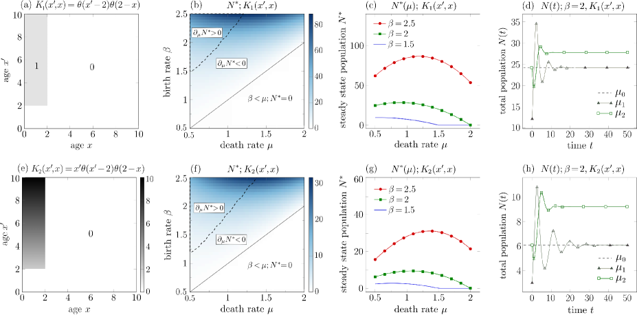
Figure 1: (a) Heatmap of the dimensionless predation interaction $K_{1}(x^{\prime},x)=\theta(x^{\prime}-2)\theta(2-x)$. (b) Heatmap of the total steady-state population $N^{*}$ as a function of constant $\beta$ and $\mu$. A nontrivial stable fixed point arises only for $\beta>\mu$. The region of no overcompensation, where $\partial_{\mu}N^{*}<0$, is indicated while the parameters that admit steady-state overcompensation, where $\partial_{\mu}N^{*}>0$ (not indicated), occur in the upper-left corner. The dashed curve delineates the phase boundary on which $\partial_{\mu}N^{*}=0$. (c) $N^{*}$ plotted as a function of $\mu$ for fixed values of $\beta=2.5,2,1.5$. (d) Plots of $N(t)$ for $\beta=2$ and death rate sequences $\mu_{1}(t)$ and $\mu_{2}(t)$ (Eq. (10)). For $\mu_{1}(t)$, damped oscillations yield transient overcompensation, while $\mu_{2}(t)$ results in a permanent, steady-state overcompensation, in addition to damped oscillations. (e-h) The corresponding results for $\beta=2$ and the predation/cannibalization interaction $K_{2}(x^{\prime},x)=x^{\prime}K_{1}(x^{\prime},x)$.

First, we investigate how the steady-state total population $N^{*}=\int_{0}^{\infty}n^{*}(x,t)\mathrm{d}x$ varies with constant $\beta$ and $\mu$. Figs. 1(b) and (f) plot $N^{*}$ and the solution to Eq. (7) using $K_{1}$ and $K_{2}$, respectively. We see that for both types of interactions, regimes in which $\partial_{\mu}N^{*}>0$ arise, signaling permanent overcompensation. In Figs. 1(b) and (f), the unlabeled overcompensation regime is in the upper left when birth rates are large and death rates small. The dashed curves Figs. 1(b) and (f) mark the “phase boundary” of overcompensation at which $\partial_{\mu}N^{*}=0$. For larger $\mu$ and smaller $\beta$, $\partial_{\mu}N^{*}<0$, and there is no overcompensation. Note that when $\beta<\mu$, the only stable state is $n^{*}(x),N^{*}=0$. Figs. 1(c) and (g) show the corresponding curves $N^{*}(\mu)$ for fixed values of $\beta$, quantitatively illustrating the different magnitudes of steady-state overcompensation through different values of the slope $\partial_{\mu}N^{*}$. These results, along with the interactions shown to preclude long-lasting overcompensation, indicate that permanent overcompensation in our model requires cannibalization of the young by the old and a $K(x^{\prime},x)$ that increases in $x^{\prime}$ and decreases in $x$.

To interrogate the dynamics of the population following perturbations to the death rate, we now start the system at its steady state corresponding to specific values $\beta_{0},\mu_{0}$ and consider how the population $N(t)$ evolves after applying these two different perturbations:

$$\mu_{1}(t)=\mu_{0}+(\log 2)\delta(t),\quad\mu_{2}(t)=\mu_{0}+\theta(t)\Delta\mu.$$ (10)

To be specific, we take $\beta_{0}=2$, $\mu_{0}=1/2$, and $\Delta\mu=1/2$. The death rate function $\mu_{1}(t)$ includes a delta function at $t=0$, which corresponds to an instantaneous removal of half the population from the steady state associated with $\beta_{0},\mu_{0}$ and the corresponding interaction $K$. A finite volume discretization (Eymard et al., 2000) with $\Delta x=0.02,x_{\max}=10,\Delta t=0.002$ was used to numerically solve Eq. (5) to find $n(x,t)$, which is then used to construct $N(t)=\int_{0}^{\infty}n(x,t)\mathrm{d}x$. Figs. 1(d) and (h) show damped oscillations in $N(t)$ associated with $K_{1}$ and $K_{2}=x^{\prime}K_{1}$, respectively. Although $\mu_{1}(t)$ immediately returns to the value $\mu_{1}(t>0)=\mu_{0}$, and $N(t\to\infty)\to N^{*}$, at shorter times, $N(t)$ oscillates and can exceed $N^{*}$ at intermediate times. Thus, transient overcompensation can arise even though the population returns to the same value set by $\beta_{0},\mu_{0}$. If $\mu_{2}(t)$ is used, the death rate jumps from $\mu_{0}$ to $\mu_{0}+\Delta\mu$ at $t=0$, leading ultimately to a higher steady-state population. For $\mu_{2}$, in addition to a higher steady-state population, initial oscillations can lead to even higher transient populations.

Motivated by these results showing that $N^{*}$ can increase upon increasing $\mu$ for fixed values of $\beta$, we provide in Appendix E additional examples of mechanisms whereby a steady-state overcompensation can arise. First, we consider overcompensation in a model in which $R(x^{\prime},x)=K(x,x^{\prime})/4$ and the birth rate function that models predation-enhanced fecundity takes on the form $\beta(x,\phi[n;x])=\beta_{0}+\phi[n;x]/4$. In this example, $\beta(x,\phi[n;x])=\beta_{0}+(\tfrac{1}{4})\int_{0}^{\infty}\!\!K(x,x^{\prime})n(x^{\prime},t)\mathrm{d}{x^{\prime}}$ is shown to preserve overcompensation associated with increases in $\mu$, as detailed in Appendix E.1.

We also show in Appendix E.2 that age-dependent harvesting can lead to overcompensation. Harvesting or culling of the population that is modeled via an additional removal term

$$\frac{\partial n(x,t)}{\partial t}+\frac{\partial n(x,t)}{\partial x} =-\left[\mu(x,t)+\int_{0}^{\infty}\!\!K(x^{\prime},x)n(x^{\prime},t)\mathrm{d}{y}\right]n(x,t)-h(n;x,t),$$ (11)

$$n(0,t) =\int_{0}^{\infty}\!\!\beta(x)n(x,t)\mathrm{d}{x},$$

where $h(n;x,t)$ represents the rate of harvesting that may depend nonlinearly on the structured population. Increases in a realistic harvesting function $h(n;x,t)$ are shown to lead to permanent increases in the total population. Finally, we also prove in Appendix E.3 that for an interaction that satisfies Eq. (8), increasing a constant $\beta$ will always lead to an increase in $N^{*}$; however, for asymmetric predation kernels that can be negative (a young-eat-old interaction), overcompensation in response to increased birth rates, where $\partial_{\beta}N^{*}<0$ for fixed values of $\mu$, can arise.

3.4 Undamped oscillations

The instantaneous changes in the death rate given by Eqs. (10) and the interactions $K_{1}$ and $K_{2}$ give rise to damped oscillations that eventually settle back to their corresponding unique values $N^{*}$. However, oscillations may be undamped and lead to periodic overcompensation when the fixed point loses stability and bifurcates to a stable limit cycle. Such oscillations have been observed, for example, in European green crabs populations (Grosholz et al., 2021). Although the source of such oscillations may be difficult to disentangle from the effects of seasonality, they have been modeled in different contexts using a single-compartment discrete-time population model (Boyce et al., 1999). Overcompensation has also been described in consumer-resource models, as cycles of rising and falling populations (Pachepsky et al., 2008), as in the classical predator-prey model.

Here, we use a simple, realistic old-eat-young cannibalization rate

$$K_{3}(x^{\prime},x)=(x^{\prime}-x)\theta(x^{\prime}-2)\theta(2-x)$$ (12)

and assume constant birth rate $\beta$ and death rate $\mu$. Upon numerically solving Eq. (5) using a finite volume discretization with $\Delta x=0.01,\Delta t=0.002$ and initial condition $n(x,0)=e^{-2x}/2$, we explore whether or not the total population $N(t)$ oscillates.

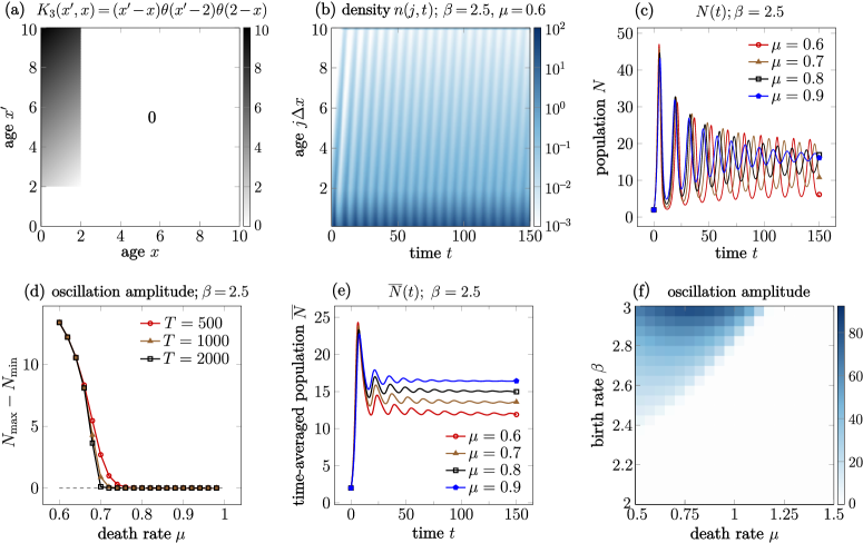
Figure 2: (a) Heatmap of the interaction kernel $K_{3}(x^{\prime},x)=(x^{\prime}-x)\theta(x^{\prime}-2)\theta(2-x)$ (Eq. (12)). (b) The population density computed using Eq. (12), $\beta=2.5$, and $\mu=0.6$, and approximated as $n(j,t)\equiv(\Delta x)^{-1}\int_{j\Delta x}^{(j+1)\Delta x}n(y,t)\mathrm{d}y$ with $\Delta x=0.02$ displays persistent periodic oscillations. (c) The total population $N(t)=\int_{0}^{\infty}n(x,t)\mathrm{d}{x}$ also exhibits oscillations that persist(damp) for small(large) values of $\mu$. (d) The long-time oscillation amplitude $\max_{T-20\leq t\leq T}N(t)-\min_{T-20\leq t\leq T}N(t)$ near $T=500$, $T=1000$, and $T=2000$, respectively, plotted as a function of $\mu$ ($\beta=2.5$). As $T$ is increased, the transition to oscillating states as $\mu$ is decreased becomes sharper These numerical results suggest that the transition at $\mu\sim 0.7$ has jump discontinuity in the first-order derivative. (e) Time-averaged populations $\overline{N}(t)\equiv\tfrac{1}{t}\int_{0}^{t}N(s)\mathrm{d}{s}$ for $\beta=2.5,\mu=0.6,0.7,0.8,0.9$ that more clearly reveal the mean values of $N(t\to\infty)$. (f) Oscillation amplitude in $\beta$-$\mu$ space. As $\beta$ increases from $2$ to $3$ and $\mu$ decreases from $1.5$ to $0.5$, undamped oscillations arise. Here, the oscillation amplitudes are measured by $\max\limits_{480<t\leq 500}N(t)-\min\limits_{480<t\leq 500}N(t)$. In the regime plotted, we find that undamped oscillations arise for $\beta\gtrsim 1.87+0.93\mu$.

Fig. 2(a) shows the heatmap of the interaction kernel $K_{3}(x^{\prime},x)=(x^{\prime}-x)\theta(x^{\prime}-2)\theta(2-x)$, while Fig. 2(b) shows a heatmap of an oscillating structured population density $n(x,t)$ approximated by its local mean value $n(j,t)=(\Delta x)^{-1}\int_{j\Delta x}^{(j+1)\Delta x}n(y,t)\mathrm{d}y$. These oscillations lead to an oscillating total population $N(t)$, as shown in Fig. 2(c). Oscillations damp out when $\mu$ is large, but persist for smaller values of $\mu$. The long-time amplitudes of oscillation shown in Fig. 2(d) indicate a sharp decrease as $\mu$ is increased. To better resolve the long-time average values of $N(t)$, we define its function average $\overline{N}(t)\equiv\tfrac{1}{t}\int_{0}^{t}N(s)\mathrm{d}s$ and plot them in Fig. 2(e). Besides transient or permanent oscillations that lead to temporary overcompensation, increasing $\mu$ in the regime studied also led to increased average values of $N(t)$, and in particular, when oscillations are damped out at larger $\mu$, the steady values $N^{*}$ also increase with $\mu$. Thus, as $\mu$ increases, periodic overcompensation transitions to steady-state overcompensation. The phase diagram separating regimes of transient and permanent oscillations is shown in Fig. 2(f). As $\beta$ increases and $\mu$ decreases, the dynamics transition from a monotonically converging one (to steady-state value $N^{*}$) to a periodically oscillating one, with a finite oscillation magnitude that arises when $\beta$ exceeds a critical value $\beta_{*}\approx 1.87+0.93\mu$.

3.5 Reduction of structured population PDE to ODE systems

We have provided some numerical examples which explicitly show various types of overcompensation in response to variations in constant $\mu,\beta$. However, our model can also be approximated via coarse-graining and discretization and formulated in terms of a system of coupled nonlinear ODEs. Systems of ODEs are typically used to describe multispecies models in which previous studies have found overcompensation. Multistage models in which, e.g., adult or later-stage insect feed on eggs or early-stage individuals (Thomas and Manica, 2003; Ohba et al., 2006) can also be directly modeled by our discrete stage discretized ODEs.

Since the analysis of the general nonlinear PDE model Eq. (5) or the steady-state integral-differential equation Eq. (7) is difficult and uniqueness only under Eq. (8) and a few specific proofs of cases that preclude overcompensation could be found (see Appendix A), related analyses of the ODE system can be more easily performed (De Roos et al., 2008; Sorenson and Cortez, 2021) if parameters and variables are considered to be piecewise constants. In addition to providing mathematical insight into the approximate, lower dimensional ODE system, the simplest numerical implementation of a finite volume method for the PDE model Eq. (5) is conceptually similar to piecewise constant discretization in the age variable.

Here, we formally discretize our PDE model and explore whether the resulting ODE models exhibit the analogous behaviors of the full PDE model discussed above. We discretize the space of ages $[0,\infty)$ into $L+1$ bins: $[x_{i},x_{i+1}),~{}i=0,...,L$ where $x_{i}=i\Delta x$ if $i\leq L$, and $x_{L+1}=\infty$. Let the population on the $i^{\textrm{th}}$ bin $[x_{i},x_{i+1})$ be denoted $n_{i}(t)=\int_{x_{i}}^{x_{i+1}}n(y,t)\mathrm{d}y,\,\,(x_{L+1}\to\infty)$. By integrating Eq. (5) over increments, each $n_{i}$ obeys

$$\frac{\mathrm{d}n_{i}}{\mathrm{d}t}= \,n(x_{i},t)-n(x_{i+1},t)-\int_{x_{i}}^{x_{i+1}}\mu(x,t)n(x,t)\mathrm{d}{x}$$ (13)

$$\hskip 56.9055pt-\int_{x_{i}}^{x_{i+1}}\!\!\!\mathrm{d}x\int_{x}^{\infty}\!\!\mathrm{d}x^{\prime}\,n(x^{\prime},t)K(x^{\prime},x)n(x,t),$$

$$n(0,t)= \sum_{i=0}^{L}\int_{x_{i}}^{x_{i+1}}\!\!\beta(x)n(x,t)\mathrm{d}{x}.$$

We now take the coefficients $\beta,\mu$, and $K$ to be piecewise constant in each compartment,i.e.,

$$\beta\big{(}x,\phi[n;x],t\big{)} =\beta_{i}\big{(}\textstyle{\sum\limits_{j=1}^{L}}R\big{(}(i-\frac{1}{2})\Delta{x},(j-\frac{1}{2})\Delta{x},t\big{)}n_{i}(t)\Delta{x},t\big{)},\quad x\in[x_{i},x_{i+1}),$$ (14)

$$\mu(x,t) =\mu_{i}(t),\qquad x\in[x_{i},x_{i+1}),$$

$$K(x^{\prime},x) =K_{j,i}(t),\quad\,\,x^{\prime}\in[x_{j},x_{j+1}),\,x\in[x_{i},x_{i+1}),$$

where $\beta(x,t)=\beta_{i}(t),\,\,x\in[x_{i},x_{i+1})$ if $\beta$ is independent of cannibalism. If we approximate $n(x_{i},t)\Delta{x}\approx n_{i-1}(t),\,\,L\geq i>0$ for sufficiently smooth $n(x,t)$, Eq. (13) simplifies to

$$\frac{\mathrm{d}n_{0}}{\mathrm{d}t} =-\mu_{0}(t)n_{0}(t)-n_{0}(t)\sum_{j=0}^{L}\!K_{j,0}n_{j}(t)+\sum_{j=1}^{L}\beta_{j}(t)n_{j}(t)-\frac{n_{0}(t)}{\Delta{x}},$$ (15)

$$\frac{\mathrm{d}n_{i}}{\mathrm{d}t} =-\mu_{i}(t)n_{i}(t)-n_{i}(t)\sum_{j=i}^{L}\!K_{j,i}n_{j}(t)-\frac{n_{i}(t)-n_{i-1}(t)}{\Delta{x}},\quad\,0<i<L,$$

$$\frac{\mathrm{d}n_{L}}{\mathrm{d}t} =-\mu_{L}(t)n_{L}(t)-n_{L}(t)K_{L,L}n_{L}(t)+\frac{n_{L-1}(t)}{\Delta{x}}.$$

$K_{i,i}$ represents the within-compartment competition introduced due to the discretization. In the following, we will assume that $K_{i,i}=0$ and that $\beta_{0}=0$. Note that the ODE system Eq. (15) is also the discretized finite volume method we used to numerically solve the original PDE Eq. (5). We are particularly interested in whether the simplified ODE model Eq. (15) with time-independent coefficients gives rise to the rich dynamics observed in the original PDE model, especially as $L$ is varied. Our main results are: (i) the ODE system Eq. (15) has at most one positive steady state, (ii) the two-compartment ODE model (setting $L=1$ in Eq. (15)) has a unique positive steady state and the steady-state populations $n_{0}$ and $n_{1}$ never increase with the death rate. This result deviates from that of the two-stage ODE model in (Sorenson and Cortez, 2021) where overcompensation could occur, at least for one compartment, (iii) the three-compartment ODE model (setting $L=2$) exhibits a unique, positive, stable steady state and overcompensation of the total population can arise, and (iv) higher-$L$ ODE systems can exhibit permanent as well as oscillatory behavior as the positive steady state destabilizes. The proofs for these results are detailed in Appendix D.

4 Summary and Conclusions

In this paper, we proposed a deterministic population model that combines a continuum of Lotka-Volterra-type interactions with age structure to describe intraspecies predation or cannibalization. Distinct from previous models that typically assume complicated interactions within multistage/multispecies populations or rely on complex consumer-resource interactions, we demonstrate mathematically that our single-species, bilinear interaction model, structured simply according to age, can give rise to a variety of dynamical behavior.

With realistic forms of predation, our model can exhibit permanent, steady-state overcompensation of the total population in response to increases in death rate. General forms of predation kernels $K(x^{\prime},x)$ that preclude steady-state overcompensation were enumerated showing that gradients in both $x^{\prime}$ and $x$ are necessary for static overcompensation (when $\beta$ and $\mu$ are constants). Specifically, our analysis suggests that $K(x^{\prime},x)$ that increases in $x^{\prime}$ and decreases in $x$ are more likely to exhibit steady-state overcompensation. Using predation kernels $K_{1}(x^{\prime},x)$ and $K_{2}(x^{\prime},x)$, Eq. (5) was solved numerically using a finite volume method to show the emergence of steady-state overcompensation. Our model is also amenable to recently developed adaptive spectral methods that are quite efficient at handling unbounded domains (Xia et al., 2021a, b; Chou et al., 2023).

Our analyses also allowed us to quantitatively distinguish transient overcompensation from steady-state overcompensation. Dynamic, or transient overcompensation was defined in terms of oscillations in the total population that also arose under predation kernels $K_{1}$ and $K_{2}$ and abrupt changes in the values of $\mu$ and $\beta$ (see Fig. 1). These cases exhibited damped oscillations in the total population that transiently exceeded their expected steady-state values. At long times, the total populations converged to steady values uniquely associated with their permanent values of $\mu$. For $\mu$ that has permanently increased, steady-state overcompensation is not universal but arises only under certain values of $\beta$ and $\mu$. However, for values of $\beta$ and $\mu$ under which steady-state overcompensation does not arise (for $K=K_{1},K_{2}$), transient overcompensation may nonetheless arise following jumps in $\mu(t)$.

Using certain forms of $K$ (see Fig. 1), dynamic or transient overcompensation was observed in terms of oscillations in the total population that eventually damps to steady values that could be lower or higher (steady-state overcompensation) following increases in $\mu(x)$. However, similar to predator-prey models that can exhibit periodic oscillations, we also found that an interaction such as $K_{3}(x^{\prime},x)=(x^{\prime}-x)\theta(x^{\prime}-2)\theta(2-x)$ leads to undamped oscillations in total population for certain values of $\beta$ and $\mu$. We found numerically that permanent oscillations emerge in a way suggestive of a Hopf bifurcation as $\mu$ is decreased. It would be interesting to develop analytic results for how stability is gained or lost as $\mu$ is tuned.

Besides formal proofs that certain simple predation interactions rule out permanent overcompensation, and numerical exploration of specific cases that exhibit dynamical (damped and undamped oscillations) and steady-state overcompensation, a rigorous analysis of our nonlinear structured population PDE model remains elusive. However, simplification via coarse-graining and discretizing the age variable allowed the PDE to be cast as a system of approximating ODEs for piecewise constant parameter functions $\beta(x),\mu(x)$, and $K(x^{\prime},x)$. The corresponding system of ODEs was amenable to additional mathematical analysis. Specifically, we showed that, under certain conditions, both the original Lotka-Volterra-type PDE model and the reduced ODE model admitted at most one positive steady state, implying that permanent overcompensation associated with increases in the death rate is unlikely due to transitions from one steady state to another. Steady-state overcompensation and permanent oscillations are also recapitulated in ODE systems of at least three and four dimensions, respectively. These results may provide insight into mathematical strategies for analyzing our PDE model under age-dependent birth and death rates.

A number of additional extensions and analyses of our model are apparent. For example, since chaotic behavior can arise in the two-species predator-prey dynamics (Wikan and Kristensen, 2021), another intriguing question is how chaotic solutions might arise in our single-species continuously structure model Eq. (5), which would carry many important ecological implications. Continuously structured PDE models can also be combined wihtin multicomponent models where even richer behavior might arise. For example, multicompartment aging models with symmetric age-age interactions have been shown to give rise to waves in opinion dynamics Chuang et al. (2018). Finally, in analogy with spatial predator-prey models (Cosner et al., 1999; Cantrell and Cosner, 2001), including age-dependent spatial diffusion within our continuum structured PDE model may lead to intriguing behavior such as transport-mediated local and global overcompensation.

Declaration of interest

None

Author contributions

All authors, Mingtao Xia, Xiangting Li, and Tom Chou conceptualized the project, performed the mathematical and computational analyses, visualized the results, wrote, and edited the manuscript.

Mathematical Appendices

Appendix A Interactions that preclude permanent overcompensation

A.1 Self-inhibition $K(x^{\prime},x)=k(x)\delta(x^{\prime}-x)$

We first show that if cannibalization occurs within individuals of the same structured variable (age in this case), i.e., $K(x^{\prime},x)=k(x)\delta(x^{\prime}-x),k(x)>0$, no overcompensation can occur, even for age-dependent birth and death rates $\beta(x)$ and $\mu(x)$. The steady-state Eq. (7) becomes a Riccati equation with a specific boundary condition,

$${\mathrm{d}n^{*}(x)\over\mathrm{d}x}=-\mu(x)n^{*}(x)-k(x)(n^{*}(x))^{2},\quad n^{*}(0)=\int_{0}^{\infty}\!\!\beta(x)n^{*}(x)\mathrm{d}{x}.$$ (16)

After defining $q^{*}(x)\coloneqq k(x)n^{*}(x)$, Eq. (16) simplifies to

$$\frac{\mathrm{d}q^{*}(x)}{\mathrm{d}x}=-\hat{\mu}(x)q^{*}(x)-[q^{*}(x)]^{2},\quad\hat{\mu}(x)\coloneqq\mu(x)-\frac{k^{\prime}(x)}{k(x)},\quad q^{*}(0)=\!\int_{0}^{\infty}\!\frac{k(0)}{k(x)}\beta(x)q^{*}(x)\mathrm{d}{x}.$$ (17)

Substituting $q^{*}(x)=u^{\prime}(x)/u(x)$ into Eq. (17), we obtain the linear ODE $\frac{\mathrm{d}^{2}u(x)}{\mathrm{d}x^{2}}+\hat{\mu}(x)\frac{\mathrm{d}u(x)}{\mathrm{d}x}=0$ which admits the general solution

$$u(x)\propto\big{(}1+C\int_{0}^{x}\!e^{-\int_{0}^{z}\hat{\mu}(y)\mathrm{d}{y}}\mathrm{d}{z}\big{)},$$ (18)

where $C$ is an integration constant and it is assumed that $\hat{\mu}$ such that $\int_{0}^{z}\hat{\mu}(y)\mathrm{d}{y}$ has a finite lower bound and that $e^{-\int_{0}^{z}\hat{\mu}(y)\mathrm{d}{y}}$ is integrable. The steady-state population density $n^{*}(x)$ is then reconstructed as

$$n^{*}(x)=\frac{1}{k(x)}\frac{e^{-\int_{0}^{x}\hat{\mu}(x^{\prime})\mathrm{d}x^{\prime}}}{\tfrac{1}{C}+\int_{0}^{x}\!e^{-\int_{0}^{z}\hat{\mu}(y)\mathrm{d}{y}}\mathrm{d}{z}},\quad C=k(0)n^{*}(0).$$ (19)

Substituting Eq. (19) into Eq. (16), we find the constraint on $C=k(0)n^{*}(0)$

$$1=\int_{0}^{\infty}\frac{k(0)}{k(x)}\frac{\beta(x)e^{-\int_{0}^{x}\hat{\mu}(x^{\prime})\mathrm{d}{x^{\prime}}}}{1+C\int_{0}^{x}\!e^{-\int_{0}^{z}\hat{\mu}(y)\mathrm{d}{y}}\mathrm{d}{z}}\,\mathrm{d}{x}.$$ (20)

Suppose we have two different death rates $\mu_{1}(x)\geq\mu_{2}(x)$ (and thus $\hat{\mu}_{1}(x)\geq\hat{\mu}_{2}(x)$) with their corresponding steady-state solutions $n_{1}^{*}(x),n_{2}^{*}(x)$ defined by their integration constants $C(\mu_{1}),C(\mu_{2})$. We first show that $C(\mu_{1})>C(\mu_{2})$. Define

$$F_{\mu}(C)=\int_{0}^{\infty}\frac{k(0)}{k(x)}\frac{\beta(x)e^{-\int_{0}^{x}\hat{\mu}(x^{\prime})\mathrm{d}{x^{\prime}}}}{1+C\int_{0}^{x}\!e^{-\int_{0}^{z}\hat{\mu}(y)\mathrm{d}{y}}\mathrm{d}{z}}\,\mathrm{d}{x},$$ (21)

which is a decreasing function of $C$ when $C>0$. Next, note that

$$\frac{e^{-\int_{0}^{x}\hat{\mu}_{1}(x^{\prime})\mathrm{d}{x^{\prime}}}}{1+C\int_{0}^{x}\!e^{-\int_{0}^{z}\hat{\mu}_{1}(y)\mathrm{d}{y}}\mathrm{d}{z}}\leq\frac{e^{-\int_{0}^{x}\hat{\mu}_{2}(x^{\prime})\mathrm{d}{x^{\prime}}}}{1+C\int_{0}^{x}\!e^{-\int_{0}^{z}\hat{\mu}_{2}(y)\mathrm{d}{y}}\mathrm{d}{z}}$$ (22)

if $\mu_{1}(x)\geq\mu_{2}(x)$. Thus, $F_{\mu_{1}}(C(\mu_{1}))=1$ and $\mu_{1}(x)\geq\mu_{2}(x)$ imply $F_{\mu_{2}}(C(\mu_{1}))>1$. Together with the constraint $F_{\mu_{2}}(C(\mu_{2}))=1$ and monotonicity of $F_{\mu_{2}}$, $F_{\mu_{2}}(C(\mu_{1}))>1$ implies $C(\mu_{2})>C(\mu_{1})$; in other words, $n_{2}^{*}(0)>n_{1}^{*}(0)$. Furthermore, we have for all $x\geq 0$

$$n_{1}^{*}(x) =\frac{1}{k(x)}\frac{e^{-\int_{0}^{x}\hat{\mu}_{1}(x^{\prime})\mathrm{d}{x^{\prime}}}}{\tfrac{1}{C(\mu_{1})}+\int_{0}^{x}\!e^{-\int_{0}^{z}\hat{\mu}_{1}(y)\mathrm{d}{y}}\mathrm{d}{z}}$$ (23)

$$\leq\frac{1}{k(x)}\frac{e^{-\int_{0}^{x}\hat{\mu}_{2}(x^{\prime})\mathrm{d}{x^{\prime}}}}{\tfrac{1}{C(\mu_{2})}+\int_{0}^{x}\!e^{-\int_{0}^{z}\hat{\mu}_{2}(y)\mathrm{d}{y}}\mathrm{d}{z}}=n_{2}^{*}(x).$$

Thus, the total populations $N_{1}^{*}$ and $N_{2}^{*}$ satisfy $N_{1}^{*}=\int_{0}^{\infty}\!\!n_{1}^{*}(x)\mathrm{d}{x}\leq\int_{0}^{\infty}\!\!n_{2}^{*}(x)\mathrm{d}{x}=N_{2}^{*}$. We conclude that no overcompensation will be observed under an interaction of the form $K(x^{\prime}-x)=k(x)\delta(x^{\prime}-x)$.

A.2 $x$-independent cannibalism rate $K=K(x^{\prime})$

We also show that an $x$-independent predation (predators do not prefer prey of any age), $K(x^{\prime},x)=K(x^{\prime})$, also precludes permanent overcompensation. In this proof however, we must assume age-independent birth and death $\beta(x)=\beta,\mu(x)=\mu$. For $K(x^{\prime},x)=K(x^{\prime})$, the solution to Eq. (7) satisfies

$$n^{*}(x)=n^{*}(0)e^{-(\mu+K^{*})x},\,\,\,K^{*}\equiv\int_{0}^{\infty}\!K(x^{\prime})n^{*}(x^{\prime})\mathrm{d}{x^{\prime}},\,\,\,n^{*}(0)=\beta N^{*}=\beta\int_{0}^{\infty}n^{*}(x)\mathrm{d}x.$$ (24)

When $\mu\geq\beta$, no positive $K^{*}$ in Eq. (24) can satisfy $N^{*}=\int_{0}^{\infty}n^{*}(x)\mathrm{d}x$ and no positive solution exists. Numerical integration of the full time-dependent model in Eq. (5) shows that the only steady state is $n^{*}\equiv 0$. When $\mu<\beta$, the solution to Eq. (24) is satisfied by $K^{*}=\beta-\mu$ which leads to $n^{*}(x)=\beta N^{*}e^{-\beta x}$. Upon using $n^{*}(x)=\beta N^{*}e^{-\beta x}$ in the expression $K^{*}=\beta-\mu=\int_{0}^{\infty}\!K(x^{\prime})n^{*}(x^{\prime})\mathrm{d}x^{\prime}=\beta N^{*}\int_{0}^{\infty}K(x^{\prime})e^{-\beta x^{\prime}}\mathrm{d}x^{\prime}$, we find

$$N^{*}=\frac{1-\tfrac{\mu}{\beta}}{\int_{0}^{\infty}\!K(x^{\prime})e^{-\beta{x^{\prime}}}\mathrm{d}{x^{\prime}}},$$ (25)

which strictly decreases with $\mu$. Thus, a predation kernel that is independent of prey age $x$ cannot exhibit steady-state overcompensation.

A.3 $x^{\prime}$-independent cannibalism rate $K(x^{\prime},x)=K(x)$

For a predation/cannibalization rate of the form $K(x^{\prime},x)=K(x)$, the steady-state Eq. (7) becomes

$$\frac{\mathrm{d}n^{*}(x)}{\mathrm{d}x}=-\left[\mu+K(x)\!\int_{0}^{\infty}\!\!n^{*}(x^{\prime})\mathrm{d}{x^{\prime}}\right]n^{*}(x),\quad n^{*}(0)=\beta N^{*}.$$ (26)

We now prove that if $\mu,\beta$ are constants, then no permanent overcompensation will occur. Equation (26) is solved by $n^{*}(x)=n^{*}(0)e^{-\mu x-N^{*}\tilde{K}(x)}$, where $\tilde{K}(x)\equiv\int_{0}^{x}\!K(y)\mathrm{d}y$. Upon integrating the solution and using the boundary condition $n^{*}(0)=\beta N^{*}$, eliminating $n^{*}(0)$, and using the definition $N^{*}=\int_{0}^{\infty}\!n(x)\mathrm{d}x$, we find an implicit solution for $N^{*}$:

$$1=\beta\int_{0}^{\infty}\!\!e^{-\mu x-N^{*}\tilde{K}(x)}\mathrm{d}x\equiv F(\mu,N^{*}).$$ (27)

Eq. (27) is the specific form of Eq. (42) to be derived under a general condition later. To see how $N^{*}$ varies with $\mu$, we introduce perturbation $(\delta\mu,\delta N^{*})$ to the solution $(\mu,N^{*})$ to Eq. (27) and find

$$1=F(\mu,N^{*})+\left(\frac{\partial F}{\partial\mu}\right)\delta\mu+\left(\frac{\partial F}{\partial N^{*}}\right)\delta N^{*}+o(\delta\mu,\delta N^{*}).$$ (28)

On the lowest order, $\big{(}\partial F/\partial\mu\big{)}\delta\mu+\big{(}\partial F/\partial N^{*}\big{)}\delta N^{*}=0$, which yields

$$\frac{\delta N^{*}}{\delta\mu}=-\frac{(\partial F/\partial\mu)}{(\partial F/\partial N^{*})}=-\frac{\int_{0}^{\infty}\!xe^{-\mu x-N^{*}\tilde{K}(x)}\mathrm{d}x}{\int_{0}^{\infty}\!\tilde{K}(y)e^{-\mu y-N^{*}\tilde{K}(y)}\mathrm{d}y}.$$ (29)

For $\mu,N^{*}>0$, the RHS above is negative. Thus, $\partial N^{*}/\partial\mu<0$ and steady-state overcompensation cannot arise. This result implies that an interaction kernel $K(x^{\prime},x)$ that varies only in $x$ is insufficient for steady-state overcompensation and that variation in $x^{\prime}$ is necessary. This result, along with that in section A.2, suggests that predation kernels $K(x^{\prime},x)$ that vary in both $x^{\prime}$ and $x$ are required for steady-state overcompensation, at least for age-independent $\beta$ and $\mu$.

Appendix B Uniqueness of the positive steady state of Eq. (5)

If the distributed interaction $K(x^{\prime},x)$ satisfies Eq. (8), we shall prove uniqueness of a positive steady state under the assumption that the set $\{x:\exists x^{\prime}>x>0,K(x^{\prime},x)>0\}\cap\{x:\beta(x)>0,x>0\}$ has positive measure. First, we assume two steady states, $m^{*}(x)$ and $n^{*}(x)$, and demonstrate that if $m^{*}(X)=n^{*}(X)$ at some age $X$, then $m^{*}(x)$ and $n^{*}(x)$ are precisely the same steady state everywhere. Second, without loss of generality, if $n^{*}(X)>m^{*}(X)$, we will demonstrate that $n^{*}(x)>m^{*}(x)\,\,\forall x\geq 0$. This dominance relation conflicts with the well-known Euler-Lotka equation, thereby demonstrating the uniqueness of the steady-state solution.

To show

$$m^{*}(X)=n^{*}(X)\Rightarrow m^{*}(x)=n^{*}(x),\forall x\geq X,$$ (30)

first note that since $K(x^{\prime},x>X)=0$, the interaction terms in Eq. (7) for both $m(x)$ and $n(x)$ vanish for $x>X$ and thus are linear first-order equations with identical decay rates $\mu(x)$ and coincident “initial conditions” $m^{*}(X)=n^{*}(X)$. Thus, the solutions for $x>X$ are identical.

What remains is to show that $m^{*}(X)=n^{*}(X)\Rightarrow m^{*}(x)=n^{*}(x),\,\forall x\geq 0$. To simplify notation, we set $\xi=X-x$, $\xi^{\prime}=X-x^{\prime}$ and define $f(\xi)\equiv n(X-x)$, $f^{*}(\xi)\equiv n^{*}(X-x)$, transforming the steady-state problem Eq. (7) into a general integral-differential equation with given initial data (using Eq. (30))

$$\begin{cases}\displaystyle{\mathrm{d}f(\xi)\over\mathrm{d}\xi}=\left[\mu(\xi)+\int_{-\infty}^{\xi}\!\!K(\xi^{\prime},\xi)f(\xi^{\prime})d\xi^{\prime}\right]f(\xi),\;X\geq\xi>0,\\[13.0pt] f(\xi)=f^{*}(\xi),\;\forall\,\xi\leq 0,\end{cases}$$ (31)

where we have reparameterized $\mu(x)$ such that $\mu(\xi)=\mu(x=X-\xi)$ and $K(x^{\prime},x)$ such that $K(\xi^{\prime},\xi)=K(x^{\prime}=X-\xi^{\prime},x=X-\xi)$. The goal is to march the steady-state uniqueness from $\xi<0$ ($x>X$) up to $\xi=X$ ($x=0$). Let us assume that uniqueness of $f(\xi)$ has been demonstrated up to $\xi_{0}$, i.e., that $f(\xi)=f^{*}(\xi)\equiv n^{*}(X-\xi)$ has been uniquely determined in $(-\infty,\xi_{0}]$. Breaking up the integral term, we write

$$\begin{cases}\displaystyle{\mathrm{d}f(\xi)\over\mathrm{d}\xi}=\left[\mu(\xi)+\int_{-\infty}^{\xi_{0}}\!\!K(\xi^{\prime},\xi)f(\xi^{\prime})\mathrm{d}\xi^{\prime}+\int_{\xi_{0}}^{\xi}\!K(\xi^{\prime},\xi)f(\xi^{\prime})\mathrm{d}\xi^{\prime}\right]f(\xi),&\forall\,\xi>\xi_{0}\\[13.0pt] f(\xi)=f^{*}(\xi),&\forall\xi\leq\xi_{0}.\end{cases}$$ (32)

We can march $\xi_{0}$ forward from 0 and consider a small region $(\xi_{0},\xi_{0}+\varepsilon)$ successively. At each stage, since $f(\xi)=f^{*}(\xi_{0}\leq\xi<\xi_{0}+\varepsilon)$ has been uniquely determined, we can combine $\mu(\xi)+\int_{-\infty}^{\xi_{0}}K(\xi^{\prime},\xi)f(\xi^{\prime})\mathrm{d}\xi^{\prime}\to\mu(\xi)$. If we start at $\xi_{0}=0$, it suffices to show that the solution to

$$\frac{\mathrm{d}f(\xi)}{\mathrm{d}\xi}=\left[\mu(\xi)+\int_{0}^{\xi}\!K(\xi^{\prime},\xi)f(\xi^{\prime})\mathrm{d}\xi^{\prime}\right]f(\xi),\,\,\,\forall\xi>0\,\,\,f(0)=f^{*}(0)$$ (33)

is unique in a small domain of $(0,\varepsilon)$.

Suppose that $\mu(\xi)$ is (locally) bounded by $\hat{\mu}$, $K(\xi^{\prime},\xi)$ is bounded by $\hat{K}$, and $g$ is the local solution to the associated differential equation

$$\frac{\mathrm{d}g(\xi)}{\mathrm{d}\xi}=\left[\hat{\mu}+\hat{K}\int_{0}^{\xi}g(\xi^{\prime})\mathrm{d}\xi^{\prime}\right]g(\xi),\forall\xi>0,\,\,\\ g(0)=f^{*}(0).$$ (34)

The integral $G(\xi)\equiv\int_{0}^{\xi}g(\xi^{\prime})\mathrm{d}\xi^{\prime}$ then obeys the standard-form second-order ODE

$$\frac{\mathrm{d}^{2}G(\xi)}{\mathrm{d}\xi^{2}}=\left[\hat{\mu}+\hat{K}G(\xi)\right]\frac{\mathrm{d}G(\xi)}{\mathrm{d}\xi},\forall\xi>0,\,\,G(0)=0,\,\,\frac{\mathrm{d}G(\xi)}{\mathrm{d}\xi}\bigg{|}_{\xi=0}=g(0)\equiv f^{*}(0).$$ (35)

The solution to Eq. (35) in the region $(0,\varepsilon)$ is unique and for any solution $f$ of Eq. (33), $0<f\leq g$.

Now suppose that $f_{1}$ and $f_{2}$ are two solutions in the neighborhood of $0$ that solve Eq. (33). We have

$$f_{i}(\xi)=f^{*}(\xi)+\int_{0}^{\xi}\bigg{(}\mu(\xi^{\prime})+\int_{0}^{\xi^{\prime}}\!K(\xi^{\prime\prime},\xi^{\prime})f_{i}(\xi^{\prime\prime})\mathrm{d}\xi^{\prime\prime}\bigg{)}f_{i}(\xi^{\prime})d\xi^{\prime},\,\,\,i=1,2.$$ (36)

Note that

$$\begin{split}&\left|f_{1}(\xi^{\prime})\int_{0}^{\xi^{\prime}}\!K(\xi^{\prime\prime},\xi^{\prime})f_{1}(\xi^{\prime\prime})\mathrm{d}\xi^{\prime\prime}-f_{2}(\xi^{\prime})\int_{0}^{\xi^{\prime}}\!K(\xi^{\prime\prime},\xi^{\prime})f_{2}(\xi^{\prime\prime})\mathrm{d}\xi^{\prime\prime}\right|\\ &\hskip 39.83368pt=\left|f_{1}(\xi^{\prime})\int_{0}^{\xi^{\prime}}\!K(\xi^{\prime\prime},\xi^{\prime})\big{[}f_{1}(\xi^{\prime\prime})-f_{2}(\xi^{\prime\prime})\big{]}\mathrm{d}\xi^{\prime\prime}+\big{[}f_{1}(\xi^{\prime})-f_{2}(\xi^{\prime})\big{]}\int_{0}^{\xi^{\prime}}\!K(\xi^{\prime\prime},\xi^{\prime})f_{2}(\xi^{\prime\prime})\mathrm{d}\xi^{\prime\prime}\right|\\ &\hskip 39.83368pt\leq 2\hat{K}\xi^{\prime}\sup_{\xi\in(0,\varepsilon)}g(\xi)\sup_{\xi\in(0,\varepsilon)}|f_{1}(\xi)-f_{2}(\xi)|.\end{split}$$ (37)

Then, using Eq. (36), we conclude that

$$\sup_{xi\in[\xi_{0},\xi_{0}+\varepsilon]}\left|f_{1}(\xi)-f_{2}(\xi)\right|\leq\bigg{\{}\varepsilon\hat{\mu}+\varepsilon^{2}\hat{K}\sup_{\xi\in(0,\varepsilon)}g(\xi)\bigg{\}}\sup_{\xi\in[\xi_{0},\xi_{0}+\varepsilon]}\left|f_{1}(\xi)-f_{2}(\xi)\right|.$$ (38)

$\varepsilon$ can be chosen sufficiently small such that $\big{\{}\varepsilon\hat{\mu}+\varepsilon^{2}\hat{K}\sup_{\xi\in(0,\varepsilon)}g(\xi)\big{\}}<1$, so we conclude $\sup_{\xi\in[\xi_{0},\xi_{0}+\varepsilon]}\left|f_{1}(\xi)-f_{2}(\xi)\right|=0$, proving the solution to Eq. (33) is unique in a neighborhood of $0$. Under the assumption that the solution to Eq. (33) exists, we can replace the point $\xi=0$ with $\xi\in(0,K)$ and conclude that the solution is unique in a small neighborhood of $\xi$. Therefore, the solution is globally unique in $(0,K)$, and the proof of the first statement is completed.

Next, we show that the case $n^{*}(X)>m^{*}(X)$ cannot not hold by first claiming that

$$n^{*}(X)>m^{*}(X)\Rightarrow n^{*}(x)>m^{*}(x),\,\,\forall x\geq 0.$$ (39)

We easily observe that the statement is true for $x\geq X$. Suppose for some $x_{0}$, $n^{*}(x_{0})\leq m^{*}(x_{0})$. Then let $x^{*}=\sup_{x\geq 0}\{x:n^{*}(x)\leq m^{*}(x)\}$. By continuity of $m^{*}$ and $n^{*}$, we note that $x^{*}<X$.

Within the interval $(x^{*},X)$, $n^{*}(x)>m^{*}(x)$. Let $\xi^{*}=X-x^{*}$, and consider the functions $m^{*}$ and $n^{*}$ written as functions of $\xi$. The difference of Eq. 31 satisfied by $m^{*}$ and $n^{*}$ becomes

$$\frac{\mathrm{d}}{\mathrm{d}\xi}\left(n^{*}(\xi)-m^{*}(\xi)\right)\geq{\mu(\xi)}\left(n^{*}(\xi)-m^{*}(\xi)\right),\;\forall\xi\in(0,\xi^{*}).$$ (40)

By integrating both sides of Eq. (40) from $0$ to $\xi^{*}$, we conclude that $n^{*}(\xi^{*})-m^{*}(\xi^{*})>0$, which demonstrates the dominance relation $n^{*}(x)>m^{*}(x),\,\forall x\geq 0$.

We can now exploit the equilibrium form of the Euler-Lotka equation (Keyfitz and Keyfitz, 1997; Sharpe and Lotka, 1911). Let $\tilde{\mu}(x)=\mu(x)+\int_{x}^{\infty}K(x^{\prime},x)n^{*}(x^{\prime})dx^{\prime}$ be the effective death rate and $s(x)=\exp\left(-\int_{0}^{x}\tilde{\mu}(x^{\prime})\mathrm{d}x^{\prime}\right)$ be the survival probability of any individual up to age $x$. The overall steady-state rate of new births defined by

$$n(0,t)\equiv B(t)=\int_{0}^{\infty}\!\!\beta(x)n(x,t)\mathrm{d}x$$ (41)

can be formally written in terms of $s(x)$ and the form of the method of characteristics solution $n(x<t,t)=n(0,t-x)s(x)=B(t-x)s(x)$. Using this form of $n(x<t,t)$ in the integrand in Eq. (41), we find in the $t\to\infty$ limit $B(t)=\int_{0}^{\infty}\!\!\beta(x)B(t-x)s(x)\mathrm{d}x$. Since in the $t\to\infty$ steady state limit all quantities are independent of time, $B(t)=B$ and

$$1=\int_{0}^{\infty}\!\!\beta(x)s(x)\mathrm{d}x\equiv\int_{0}^{\infty}\!\!\beta(x)e^{-\int_{0}^{x}\tilde{\mu}(x^{\prime})\mathrm{d}x^{\prime}}\mathrm{d}x,$$ (42)

which means that at steady state, the population $n^{*}(x)$ and effective death rate $\tilde{\mu}(x^{\prime})$ settles to value such that the effective reproductive number $R_{0}\equiv\int_{0}^{\infty}\!\!\beta(x)s(x)\mathrm{d}x=1$.

Equation (42) must be satisfied at steady state but allows us to compare different $\tilde{\mu}$s associated with different steady state solutions. For different steady states $m^{*}$ and $n^{*}$ such that $m^{*}>n^{*}$ at all ages, the effective death rates satisfy $\tilde{\mu}^{(m)}\geq\tilde{\mu}^{(n)}$. Since $\beta$ remains the same, the survival probability satisfies $s^{(m)}\leq s^{(n)}$, where the inequality should hold on a positive measure interval. Because $\{x:\exists x^{\prime}>x>0,K(x^{\prime},x)>0\}\cap\{x:\beta(x)>0,x>0\}$ has positive measure, we will conclude

$$1=\int_{0}^{\infty}\!\!\beta(x)e^{-\int_{0}^{x}\tilde{\mu}^{(m)}(x^{\prime})\mathrm{d}x^{\prime}}\mathrm{d}x<\int_{0}^{\infty}\!\!\beta(x)e^{-\int_{0}^{x}\tilde{\mu}^{(n)}(x^{\prime})\mathrm{d}x^{\prime}}\mathrm{d}x=1.$$ (43)

This contradiction shows that if $K$ is continuous and compactly supported and if $\{x:\exists x^{\prime}>x>0,K(x^{\prime},x)>0\}\cap\{x:\beta(x)>0,x>0\}$ has positive measure, then Eq. (5) admits at most one positive steady state.

Appendix C Existence of a positive steady state of Eq. (5)

If a predation kernel satisfies Eq. (8), we can also obtain the criterion for the existence of a positive steady state, which is equivalent to finding a positive solution $n^{*}(x)$ to Eqs. (7) under certain additional assumptions.

In Appendix B, we showed that any solution $n^{*}(x)$ to Eqs. (7) must satisfy Eq. 33 with the transformed coordinate $\xi=X-x$ and $f(\xi)=n^{*}(X-x)$. For the existence arguments, we first investigate the condition under which Eq. (33) has a positive solution. Formally, we pick the initial condition $n_{X}\coloneqq f(0)>0$ as the parameter of interest, and consider the domain of $n_{X}$ such that the solution to Eq. 33 exists up to $\xi=X$. Define $f_{-1}(\xi)\equiv 0$ and $f_{n+1}(\xi)$ as solution to the ODE

$$\frac{1}{f_{n+1}(\xi)}\frac{\mathrm{d}f_{n+1}}{\mathrm{d}\xi}(\xi) =\mu(\xi)+\int_{0}^{\xi}K(\xi^{\prime},\xi)f_{n}(\xi^{\prime})\mathrm{d}\xi^{\prime},\;\forall\xi\in(0,X);$$ (44)

$$f_{n+1}(0) =n_{X},$$

where $n\geq-1$. In particular, $f_{0}(\xi)=n_{X}e^{\int_{0}^{\xi}\mu(\xi^{\prime})\mathrm{d}\xi^{\prime}}>0=f_{-1}(\xi)$ for all $\xi\in(0,X)$. For each $n$, an iterative argument shows that $f_{n}$ is bounded, continuous, and nonnegative on $[0,X]$. In addition, $f_{0}(\xi)>f_{-1}(\xi),\forall\xi\in(0,X)$ implies that $\{f_{n}(\xi)\}$ is a monotonically increasing sequence in both $\xi$ and $n$. Therefore, $f(\xi):=\lim_{n\rightarrow\infty}f_{n}(\xi)\in{(0,\infty]}$ exists and satisfies Eq. (33) up to the moment of blowup $\xi^{*}\equiv\sup\left\{\xi\in(0,X):f(\xi)<\infty\right\}$, thanks to the monotone convergence theorem.

We also observe that $f(\xi)$ depends monotonically on the initial value $n_{X}$. For sufficiently regular $\mu$ and $K$, we also assume that $f(\xi)$ depends continuously on $n_{X}$. Define the upper limit for $n_{X}$ by $n_{X}^{*}\equiv\sup\left\{n_{X}:\xi^{*}(n_{X})>X\right\}$ with the convention that $\sup\emptyset=0$, and we find an open domain $(0,n_{X}^{*})$ of $n_{X}$ such that $f(\xi)<\infty$ for all $\xi\in[0,X]$ with the initial value $n_{X}$. In particular, the continuity assumption implies $\lim_{n_{X}\rightarrow n_{X^{-}}^{*}}f(X)=\infty$. The marginal case $n_{X}^{*}=\infty$ is covered by this equation because $f(X)\geq f(0)=n_{X}\rightarrow\infty$.

Now, we recover $n^{*}(x)$ from $f(\xi)$ and denote $n^{*}$ by $n^{*}_{n_{X}}$ to emphasize the dependence on $n_{X}$. For the sake of simplicity, we assume the upper limit $n_{X}^{*}=+\infty$ in the following discussion. This can be achieved by imposing proper restrictions on $\mu$ and $K$, such that the existence of the solution to Eq. 35 on the interval $(0,X)$ is guaranteed.

We proved that there is a unique solution $n^{*}_{n_{X}}(x)$ to the first equation in Eqs. (7) when $n^{*}_{n_{X}}(X)=n_{X}$ provided that $\mu$ and $K$ are bounded on $[0,X]$, there exist positive constants $\mu_{0},K_{0}>0$ such that $\mu\geq\mu_{0},K\geq K_{0}$, and $K$ vanishes for $x>X$. We shall show that the solution to Eqs. (7) exists if: (i) in the cannibalism-free environment ($K=0$), the expected number of offspring that an individual will give birth to is larger than 1

$$\int_{0}^{\infty}\!\!\beta(x)e^{-\int_{0}^{x}\mu(x^{\prime})\mathrm{d}x^{\prime}}\mathrm{d}x>1,$$ (45)

and (ii) given any $\frac{\mathrm{d}G(\xi)}{\mathrm{d}\xi}|_{\xi=0}\coloneqq n_{X}$,

the second order ODE Eq. (35) can be solved up to $\xi=X$, and that $\frac{\mathrm{d}G(\xi)}{\mathrm{d}\xi},\xi\in(0,X)$ depends continuously on the initial $\frac{\mathrm{d}G(\xi)}{\mathrm{d}\xi}|_{\xi=0}$.

The existence of the solution to Eqs. (7) is then converted to finding a proper $n_{X}$ such that $n^{*}_{n_{X}}(0)$ is suitable for the second equation in Eqs. (7), i.e., the boundary condition representing the newborn cells. So we need to show that $\frac{\mathrm{d}G(\xi)}{\mathrm{d}\xi}|_{\xi=X}=n^{*}_{n_{X}}(0)$ satisfies the boundary condition in Eqs. (7). Note that as long as $n_{X}>0$, $n^{*}_{n_{X}}(x)>0,~{}\forall x\geq 0$. Let $\tilde{\mu}$ denote the effective death rate $\tilde{\mu}(x)=\mu(x)+\int_{x}^{\infty}K(x^{\prime},x)n^{*}_{n_{X}}(x)\mathrm{d}{x}$, then the second equation in Eqs. (7) is equivalent to

$$n^{*}_{n_{X}}(0)\left\{1-\int_{0}^{\infty}\!\!\beta(x)e^{-\int_{0}^{x}\tilde{\mu}_{n_{X}}(x^{\prime})\mathrm{d}x^{\prime}}\mathrm{d}x\right\}=0.$$ (46)

We define the Euler-Lotka functional as

$$\textrm{EL}\big{[}n^{*}_{n_{X}}\big{]}=\int_{0}^{\infty}\!\!\beta(x)e^{-\int_{0}^{x}\tilde{\mu}_{n_{X}}(x^{\prime})\mathrm{d}x^{\prime}}\mathrm{d}x,$$ (47)

Then, the second equation in Eq. (7) is equivalent to the famous Euler-Lotka equation $\textrm{EL}\big{[}n^{*}_{n_{X}}\big{]}=1$ for positive solutions $n^{*}_{n_{X}}$. We’ve shown that $n_{X}<n_{X}^{\prime}\Rightarrow\tilde{\mu}_{n_{X}}(x)\leq\tilde{\mu}_{n_{X}^{\prime}}(x),~{}\forall x\geq 0$. Therefore, the function $n_{X}\mapsto\textrm{EL}\big{[}n_{n_{X}}^{*}\big{]}$ is monotonically decreasing. Because $n^{*}_{n_{X}}(x),\,x\leq X$ depends continuously on $n^{*}_{n_{X}}$, the functional Eq. (47) also depends continuously on $n^{*}_{n_{X}}$. Consequently, we conclude that the existence of the positive steady state is equivalent to

$$\lim_{n_{X}\rightarrow\infty}\int_{0}^{\infty}\!\beta(x)e^{-\int_{0}^{x}\tilde{\mu}_{n_{X}}(x^{\prime})\mathrm{d}x^{\prime}}\mathrm{d}x <1;\quad\lim_{n_{X}\rightarrow 0+}\int_{0}^{\infty}\!\beta(x)e^{-\int_{0}^{x}\tilde{\mu}_{n_{X}}(x^{\prime})\mathrm{d}x^{\prime}}\mathrm{d}x >1.$$ (48)

When $n_{X}=0$, $n^{*}_{n_{X}}(x)\equiv 0$. Furthermore, for $x<X$, $n^{*}(x)\geq n^{*}(X)$, which implies $\lim_{n_{X}\rightarrow\infty}n^{*}_{n_{X}}(x)=\infty,x<X$. Since we have assumed that both $\mu$ and $K$ have positive lower bounds on their support and that the solution $n^{*}_{n_{X}}$ is continuously dependent on the initial condition $n_{X}$, we could conclude that

$$\lim_{n_{X}\rightarrow 0+}\tilde{\mu}_{n_{X}}(x) =\mu(x)+\int_{x}^{\infty}K(x^{\prime},x)n^{*}_{0}(x^{\prime})\mathrm{d}x^{\prime}=\mu(x);$$ (49)

$$\lim_{n_{X}\rightarrow\infty}\tilde{\mu}_{n_{X}}(x) =\mu(x)+\int_{x}^{\infty}K(x^{\prime},x)n_{\infty}^{*}(x^{\prime})\mathrm{d}x=\begin{cases}\mu(x)&x\geq X\\ \infty&\textrm{ otherwise}\end{cases}.$$

The first equation in Eq. (48) is satisfied as

$$\lim_{n_{X}\rightarrow\infty}\int_{0}^{\infty}\!\beta(x)e^{-\int_{0}^{x}\tilde{\mu}_{n_{X}}(x^{\prime})\mathrm{d}x^{\prime}}\mathrm{d}x=0$$ (50)

because $\lim_{n_{X}\rightarrow\infty}\tilde{\mu}_{n_{X}}(x)=\infty,x\in(0,X)$. Furthermore, the second equation in Eq. (48) is satisfied by the assumption Eq. (45). Therefore, there must exist an $n_{X}$ such that ${\rm EL}\big{[}n_{n_{X}}^{*}\big{]}=1$, and thus the corresponding $n_{n_{X}}(x)$ satisfies the two equations in Eqs. (7).

Appendix D Analysis of the discretized ODE system Eq. (15)

D.1 Uniqueness of the positive equilibrium of the ODE Eq. (15)

We shall first show that there is at most one positive steady-state solution $\{n_{i}^{*}\}$ of the discretized ODE Eq. (15). The positive steady-state solution to Eq. (15), if it exists, satisfies the backward difference equation:

$$n_{i-1}^{*} =\big{[}1+\Delta{x}\mu_{i}+\Delta{x}\sum_{j\geq i}K_{j,i}n_{j}^{*}\big{]}n_{i}^{*} 1<i\leq L-1$$ (51)

$$n_{L-1}^{*} =\Delta{x}(\mu_{L}+K_{L,L}n_{L}^{*})n_{L}^{*}$$ (52)

$$\sum_{i=1}^{L}\beta_{i}n_{i}^{*} =\mu_{0}n_{0}^{*}+n_{0}^{*}(\sum_{j=0}^{L}K_{j,i}n_{j}^{*})+\frac{n_{0}^{*}}{\Delta{x}}.$$ (53)

We proceed by showing that if $\{m_{i}^{*}\}$ and $\{n_{i}^{*}\}$ are two positive steady states, then $m_{L}^{*}=n_{L}^{*}$. If $m_{L}^{*}=n_{L}^{*}$, then by induction, $m_{i}^{*}\equiv n_{i}^{*}$. If $n_{L}^{*}>m^{*}_{L}$, then $n_{L-1}^{*}>m_{L-1}^{*}$ by Eq. 52. Since $K_{i,j}\geq 0$, we observe that $K_{L-1,L}n_{L}^{*}\geq K_{L-1,L}m_{L}^{*}$. This inequality further demonstrates that $n_{L-2}^{*}>m_{L-2}^{*}$ combined with Eq. 51. Thus, by induction, $n_{L}^{*}>m^{*}_{L}$ leads to $n_{i}^{*}>m_{i}^{*}$ for all $i\in\left\{0,1,...,L\right\}$.

Next, let $n_{i}(t)$ be solutions to Eq. 15 with the initial value equal to the steady state $n_{i}^{*}$. Let $B(t)\coloneqq\sum_{i}\beta_{i}n_{i}(t)$ be the newborn population at time $t$. Then, for any compartment $i$, the population $n_{i}(t)$ at time $t$ is composed of two parts: the survivors from the initial $t=0$ population and those who were born in $(0,t)$. In order to characterize survival, we define $\{s_{j,i}(t)\}_{j=0}^{L}$ to be the solution of

$$\frac{\mathrm{d}s_{i,0}(t)}{\mathrm{d}t} =-\mu_{0}s_{i,0}(t)-s_{i,0}(t)\sum_{j=0}^{L}\!K_{j,0}n_{j}(t)-\frac{s_{i,0}(t)}{\Delta{x}},$$ (54)

$$\frac{\mathrm{d}s_{i,j}(t)}{\mathrm{d}t} =-\mu_{i}s_{i,j}(t)-s_{i,j}(t)\sum_{j^{\prime}=j}^{L}\!K_{j^{\prime},j}n_{j^{\prime}}(t)+\frac{s_{i,j-1}(t)-s_{i,j}(t)}{\Delta{x}},\quad 0<j<L,$$

$$\frac{\mathrm{d}s_{i,L}(t)}{\mathrm{d}t} =-\mu_{L}s_{i,L}(t)-s_{i,L}(t)K_{L,L}n_{L}(t)+\frac{s_{i,L-1}(t)}{\Delta{x}},$$

with the initial condition $s_{i,j}(0)=1,i=j$ and $s_{ik}(0)=0,~{}\forall k\neq i$.

Note that an initial condition $n_{i}(0)=n_{i}^{*}$ implies that $n_{i}(t)=n_{i}^{*}$. Since death rates and interaction terms do not explicitly depend on time, the survival fraction is time-translation invariant, i.e., the survival from compartment $i$ at time $t=0$ to the compartment $j$ at time $t=T-\tau$ is the same as survival from compartment $i$ at time $t=\tau$ to the compartment j at time $t=T$. Therefore, the solution to Eq. 15 can be written as

$$n_{i}(t)=\sum_{j=0}^{L}n_{j}(0)s_{j,i}(t)+\int_{0}^{t}B(\tau)s_{0,i}(t-\tau)\mathrm{d}{\tau},$$ (55)

where $B(t)\coloneqq\sum_{i=0}^{L}\beta_{i}n_{i}(t)$ is the total birth rate at time $t$. Since every individual eventually dies, we have $\lim_{t\rightarrow\infty}s_{i,j}(t)=0$ for all $i,j$. Therefore, using the solution in Eq. (55) in $B(t)$, the birth rate can be decomposed into contributions from the initial population and from the population born within time $(0,t)$:

$$B(t)=\sum_{i,j=0}^{L}\beta_{j}n_{i}(0)s_{i,j}(t)+\int_{0}^{t}B(t-\tau)\sum_{i=0}^{L}\beta_{i}s_{0,i}(\tau)\mathrm{d}\tau.$$ (56)

At steady state, we introduce the lower and upper bounds of $B(t)$:

$$\int_{0}^{t}\!B(t-\tau)\sum_{i=0}^{L}\!\beta_{i}s_{0,i}(\tau)\mathrm{d}{\tau}\leq B(t)\leq\!\int_{0}^{t}\!B(t-\tau)\sum_{i=0}^{L}\!\beta_{i}s_{0,i}(\tau)\mathrm{d}{\tau}+\!\sum_{i,j=0}^{L}n^{*}_{i}\max_{i}\{\beta_{i}\}s_{i,j}(t),$$ (57)

where the left-hand side represents the birth rate at time $t$ generated by individuals born with $(0,t)$ and the right-hand side are birth rate of newborns at time $t$ that are offspring of individuals born within $(0,t)$, plus the maximum possible number of offspring that the initial population could give birth to at time $t$. When $n_{i}(0)=n_{i}^{*}$, $B(t)\coloneqq B$ is a constant and the limit $t\rightarrow\infty$ forces the lower and upper bounds to converge yielding

$$B=B\int_{0}^{\infty}\sum_{i=0}^{L}\beta_{i}s_{0,i}(\tau)\mathrm{d}{\tau},$$ (58)

which is the discrete analogue of the $R_{0}=1$ condition of Eq. (42) where the factor $\int_{0}^{\infty}\sum_{i=0}^{L}\beta_{i}s_{0,i}(\tau)\mathrm{d}{\tau}$ on the right-hand side is the expected offspring that one individual has during its lifetime.

Similar to the proof of uniqueness in Appendix B, it is intuitively clear that $s_{0,i}(a)$ as well as $\int_{0}^{\infty}\sum_{i=0}^{L}\beta_{i}s_{0,i}(\tau)\mathrm{d}{\tau}$ monotonically decreases with with increasing effective death rate $\tilde{\mu}_{i}$. We demonstrate this by explicitly computing

$$1=\int_{0}^{\infty}\sum_{i=0}^{L}\beta_{i}s_{0,i}(\tau)\mathrm{d}{\tau} =\sum_{i=1}^{L-1}\prod_{j=0}^{i-1}\frac{1}{(1+\Delta{x}\tilde{\mu}_{j})}\int_{0}^{\infty}(\tilde{\mu}_{i}+\tfrac{1}{\Delta{x}})\beta_{i}te^{-(\tilde{\mu}_{i}+1/\Delta{x})t}\mathrm{d}{t}$$ (59)

$$\qquad\quad+\prod_{j=0}^{L-1}\frac{1}{(1+\Delta{x}\tilde{\mu}_{j})}\int_{0}^{\infty}\mu_{L}\beta_{L}te^{-\tilde{\mu}_{L}t}\mathrm{d}{t},$$

$$=\sum_{i=1}^{L-1}\prod_{j=0}^{i-1}\frac{\beta_{i}\Delta x}{(1+\Delta{x}\tilde{\mu}_{j})(\Delta{x}\tilde{\mu}_{i}+1)}+\prod_{j=0}^{L-1}\frac{\beta_{L}}{\mu_{L}(1+\tilde{\mu}_{j})},$$

where $\tilde{\mu}_{i}\coloneqq\mu_{i}+\sum_{j>i}K_{j,i}n_{j}^{*}$. The first term on the right-hand side of Eq. (59) is the summation of the expected number of offspring that an individual gives birth to while in the $i^{\text{th}},\,i<L$ stage multiplied by the probability that it will survive until the $i^{\text{th}}$ stage. The second term on the right-hand side is the expected number of offspring that an individual gives birth while in the $L^{\text{th}}$ stage multiplied by the probability that it survives to the $L^{\text{th}}$ stage. If $n_{i}^{*}>m_{i}^{*},\,i=0,\ldots,L$ and there exists at least one $K_{j,i}>0$, then $\tilde{\mu}^{n}_{i}>\tilde{\mu}^{m}_{i}$ and Eq. (59) cannot be satisfied by two distinct steady-state solutions $\{m_{i}^{*}\}\neq\{n_{i}^{*}\}$.

D.2 Permanent overcompensation is precluded in two-compartment ODE models

In the following discussion, we will exclude the artificial self-inhibition term $K_{i,i}$ as a result of binning the age structure into a finite number of compartments. We start by considering the simplest two-compartment model by imposing some additional assumptions on the coefficients. Setting $L=1$ (two compartments) in Eq. (15), we find

$$\frac{\mathrm{d}n_{0}}{\mathrm{d}t}=-\mu_{0}n_{0}-K_{1,0}n_{1}n_{0}+\beta_{1}n_{1}-\frac{n_{0}}{\Delta{x}},\,\,\,\frac{\mathrm{d}n_{1}}{\mathrm{d}t}=-\mu_{1}n_{1}+\frac{n_{0}}{\Delta{x}}.$$ (60)

Eq. (60) admits a unique steady state at

$$(n_{0}^{*},n_{1}^{*})=\Big{(}\frac{\beta_{1}-\mu_{1}-\mu_{0}\mu_{1}\Delta{x}}{K_{1,0}},\frac{\beta_{1}-\mu_{1}-\mu_{0}\mu_{1}\Delta{x}}{K_{1,0}\mu_{1}\Delta{x}}\Big{)},$$ (61)

which, as is the total population $n_{0}^{*}+n_{1}^{*}$, monotonically decreasing with either $\mu_{0}$ or $\mu_{1}$, indicating that steady-state overcompensation cannot arise. The Jacobian matrix at the fixed point is

$${\bf J}=\left[\begin{array}[]{cc}\displaystyle-\mu_{0}-K_{1,0}n_{1}-\frac{1}{\Delta{x}}&\displaystyle-K_{1,0}n_{0}+\beta_{1}\\[8.0pt] \displaystyle\frac{1}{\Delta{x}}&\displaystyle-\mu_{1}\end{array}\right].$$ (62)

which has two negative eigenvalues if the equilibrium $(n_{0}^{*},n_{1}^{*})>0$. Therefore, the steady state is stable and we do not expect periodic oscillations about this fixed point.

D.3 Undamped oscillations are precluded in a three-compartment model

Setting $L=2$ in Eq. (15), we obtain

$$\frac{\mathrm{d}n_{0}}{\mathrm{d}t} =-\frac{n_{0}}{\Delta{x}}-\mu_{0}n_{0}-K_{1,0}n_{1}n_{0}-K_{2,0}n_{2}n_{0}+\beta_{1}n_{1}+\beta_{2}n_{2},$$ (63)

$$\frac{\mathrm{d}n_{1}}{\mathrm{d}t} =-\frac{n_{1}}{\Delta{x}}+\frac{n_{0}}{\Delta{x}}-\mu_{1}n_{1}-K_{2,1}n_{2}n_{1},$$

$$\frac{\mathrm{d}n_{2}}{\mathrm{d}t} =\frac{n_{1}}{\Delta{x}}-\mu_{2}n_{2}.$$

First, we demonstrate that this three-compartment model can exhibit overcompensation by considering a simple specific set of parameters: $\beta_{2}=\beta_{2}^{\prime}+\mu_{2}$, $\beta_{2}^{\prime}\geq 0$, $\mu_{1}=0$, $K_{1,0}=K_{2,1}=0$. Equations (63) then simplify to

$$\frac{\mathrm{d}n_{0}}{\mathrm{d}t} =-\frac{n_{0}}{\Delta{x}}-K_{2,0}n_{2}n_{0}+(\beta_{2}^{\prime}+\mu_{2})n_{2}+\beta_{1}n_{1},$$ (64)

$$\frac{\mathrm{d}n_{1}}{\mathrm{d}t} =\frac{n_{0}-n_{1}}{\Delta{x}},$$

$$\frac{\mathrm{d}n_{2}}{\mathrm{d}t} =\frac{n_{1}}{\Delta{x}}-\mu_{2}n_{2}$$

which admits the positive steady state

$$(n_{0}^{*},n_{1}^{*},n_{2}^{*})=(\frac{\beta_{1}\mu_{2}\Delta{x}+\beta_{2}^{\prime}}{K_{2,0}},\frac{\beta_{1}\mu_{2}\Delta{x}+\beta_{2}^{\prime}}{K_{2,0}},\frac{\beta_{1}\mu_{2}\Delta{x}+\beta_{2}^{\prime}}{\Delta{x}\mu_{2}K_{2,0}})$$ (65)

and the total steady-state population

$$N(\mu_{2})\coloneqq n_{0}^{*}+n_{1}^{*}+n_{2}^{*}=2\frac{\beta_{1}\mu_{2}\Delta{x}+\beta_{2}^{\prime}}{K_{2,0}}+\frac{\beta_{1}\mu_{2}\Delta{x}+\beta_{2}^{\prime}}{\Delta{x}\mu_{2}K_{2,0}}.$$ (66)

Therefore, $\partial_{\mu_{2}}N(\mu_{2})=\frac{2\beta_{1}\Delta{x}}{K_{2,0}}-\frac{\beta_{2}^{\prime}}{K_{2,0}\mu_{2}^{2}\Delta{x}}$ indicates that the total population at equilibrium $N(\mu_{2})$ will increase with the death rate of the oldest population $\mu_{2}$ if $\mu_{2}>\sqrt{\frac{\beta_{2}^{\prime}}{2\beta_{1}\Delta{x}^{2}}}$. So in order to observe overcompensation, at least three compartments are needed.

Next, we show that the positive steady state of the three-compartment model Eqs. (63), if it exists, is stable. This statement holds for general parameter values in Eqs. (63). The steady-state populations $n_{i}^{*}$ obey the relationships

$$n_{1}^{*} =\Delta{x}\mu_{2}n_{2}^{*},\quad n_{0}^{*}=\big{(}\Delta{x}+\mu_{1}\Delta{x}^{2}+\Delta{x}^{2}K_{2,1}n_{2}^{*}\big{)}\mu_{2}n_{2}^{*},$$ (67)

$$\Delta{x}\beta_{1}\mu_{2}+\beta_{2} =\mu_{2}\Big{(}\mu_{0}+\Delta{x}K_{1,0}\mu_{2}n_{2}^{*}+K_{2,0}n_{2}^{*}+\frac{1}{\Delta{x}}\Big{)}\big{(}\Delta{x}+\Delta{x}^{2}\mu_{1}+\Delta{x}^{2}K_{2,1}n_{2}^{*}\big{)}.$$

Therefore, this system contains one real positive fixed point whenever a positive root for $n_{2}^{*}$ satisfies the last equation in (67). This occurs for parameters values for which

$$\beta_{1}\mu_{2}\Delta x+\beta_{2}>\mu_{2}\big{(}\mu_{0}\Delta{x}+1\big{)}\big{(}\mu_{1}\Delta{x}+1\big{)}.$$ (68)

The Jacobian matrix at this fixed point is

$${\bf J}=\left[\begin{array}[]{ccc}\displaystyle-\mu_{0}-K_{1,0}n_{1}^{*}-\frac{1}{\Delta{x}}-K_{2,0}n_{2}^{*}&\displaystyle-K_{1,0}n_{0}^{*}+\beta_{1}&-K_{2,0}n_{0}^{*}+\beta_{2}\\[8.0pt] \displaystyle\frac{1}{\Delta{x}}&\displaystyle-\frac{1}{\Delta{x}}-\mu_{2}-K_{2,1}n_{2}^{*}&-K_{2,1}n_{1}^{*}\\[8.0pt] 0&\displaystyle\frac{1}{\Delta{x}}&-\mu_{2}\end{array}\right]$$ (69)

whose eigenpolynomial is

$$f(\lambda) \equiv\text{det}(\lambda\mathds{I}-{\bf J})$$ (70)

$$=\big{(}\lambda+\mu_{0}+K_{1,0}n_{1}^{*}+\frac{1}{\Delta{x}}+K_{2,0}n_{2}^{*}\big{)}\big{(}\lambda+\frac{1}{\Delta{x}}+\mu_{1}+K_{2,1}n_{2}^{*}\big{)}(\lambda+\mu_{2})+\frac{1}{\Delta{x}^{2}}(K_{2,0}n_{0}^{*}-\beta_{2})$$

$$\hskip 22.76219pt+\frac{1}{\Delta{x}}K_{2,1}n_{1}^{*}\big{(}\lambda+\mu_{0}+K_{1,0}n_{1}^{*}+\frac{1}{\Delta{x}}+K_{2,0}n_{2}^{*}\big{)}+\frac{1}{\Delta{x}}(\lambda+\mu_{2})(K_{1,0}n_{0}^{*}-\beta_{1}),$$

where $\mathds{I}$ is the identity matrix. In order to simplify this expression, we define the effective death rates to be $\tilde{\mu}_{0}=\mu_{0}+n_{1}^{*}K_{1,0}+n_{2}^{*}K_{2,0}$ and $\tilde{\mu}_{1}=\mu_{1}+n_{2}^{*}K_{2,1}$. Then, the eigenpolynomial can be simplified into

$$\begin{split}f(\lambda)=&\lambda^{3}+C_{2}\lambda^{2}+C_{1}\lambda+C_{0},\\ C_{2}&=\mu_{2}+\tilde{\mu}_{0}+\tilde{\mu}_{1}+\frac{2}{\Delta x}\\ C_{1}&=K_{1,0}n_{1}^{*}\big{(}\tilde{\mu}_{1}+\frac{1}{\Delta x}\big{)}+K_{2,1}n_{2}^{*}\mu_{2}+\mu_{2}C_{2}+\frac{\beta_{2}}{\Delta x^{2}\mu_{2}}\\ C_{0}&=\frac{\mu_{2}}{\Delta x}\big{(}K_{1,0}n_{1}^{*}\Delta x\tilde{\mu}_{1}+K_{1,0}n_{1}^{*}+K_{2,0}n_{2}^{*}\Delta x\tilde{\mu}_{1}+K_{2,0}n_{2}^{*}+K_{2,1}n_{2}^{*}\Delta x\tilde{\mu}_{0}+K_{2,1}n_{2}^{*}\big{)}\end{split}$$ (71)

Here, we have employed Eq. (67) to replace $n_{0}^{*}$, $n_{1}^{*}$, and $\beta_{1}$ by simple terms involving $n_{2}^{*}$. Note that our parameters are all non-negative. We may reasonably parameterize our model such that at least one $K_{i,j}>0$, at least one $\mu_{i}>0$, at least one $\beta_{i}>0$, and all $n_{i}^{*}>0$. Under such assumptions, $C_{0},C_{1},C_{2}>0$. Then, $f(\lambda)$ is monotonically increasing on $(0,+\infty)$. Therefore, $f(\lambda)$ has no positive real root.

What remains is to show that $f(\lambda)$ cannot have a pair of complex roots with positive real parts, which we prove by contradiction. Suppose such a pair of complex roots $\lambda_{\pm}$ exists with $\operatorname{Re}(\lambda_{\pm})>0$. Recall that $f(\lambda)$ is a polynomial of degree 3, and, from our discussion above, has a negative real root $\lambda_{1}$. $f(\lambda)$ can be factorized as $f(\lambda)=(\lambda-\lambda_{1})(\lambda^{2}+b\lambda+c)$ with $b=-(\lambda_{+}+\lambda_{-})<0$, $\lambda_{1}<0$, and $-\lambda_{1}+b=C_{2}$. Thus, $\lambda_{1}<-C_{2}$ and because $f(\lambda)$ is monotonically increasing in $(-\infty,-C_{2})$, $f(-C_{2})\geq f(\lambda_{1})=0$.

We next demonstrate the polynomial $-f(-\lambda-C_{2})=\lambda^{3}+D_{2}\lambda^{2}+D_{1}\lambda^{1}+D_{0}$ is monotonically increasing for $\lambda>0$ and that $D_{0}>0$. Through straightforward algebra, we note that $D_{2}=2C_{1}>0$, $D_{1}=C_{2}^{2}+C_{1}>0$, $D_{0}=C_{1}C_{2}-C_{0}>0$. To see $D_{0}>0$, we just claim that every term in $C_{0}$ can be written as one term in the product $C_{1}C_{2}$. For example, the first term $K_{1,0}n_{1}^{*}\tilde{\mu}_{1}\mu_{2}$ in $C_{0}$ can be written as the product of the $K_{1,0}n_{1}^{*}\tilde{\mu}_{1}$ term from $C_{1}$ and the $\mu_{2}$ term from $C_{2}$. Also note that every term in $C_{1}$ and $C_{2}$ is positive. Thus, we have $D_{0}>0$. We conclude that $f(-C_{2})<0$. This contradicts $f(-C_{2})\geq f(\lambda_{1})=0$ and precludes complex roots $\lambda_{\pm}$ with positive real parts.

Combining previous uniqueness statement and stability analysis, the system Eq. (63) admits at most one positive steady state which must be stable. Therefore, a three-compartment model precludes oscillatory solutions in the total population since the positive steady state is stable.

D.4 Higher-order reduced ODE models

For higher-order ODE models with $L+1,L\geq 2$ compartments, we can consider the special case

$$\left\{\begin{aligned} &\frac{\mathrm{d}n_{0}}{\mathrm{d}t}=-\frac{n_{0}}{\Delta{x}}-K_{L,0}n_{0}n_{L}+\beta_{1}n_{1}+(\beta_{L}^{\prime}+\mu_{L})n_{L},\\ &\frac{\mathrm{d}n_{i}}{\mathrm{d}t}=\frac{n_{i-1}-n_{i}}{\Delta{x}},~{}i=1,2...,L-1,\\ &\frac{\mathrm{d}n_{L}}{\mathrm{d}t}=\frac{n_{L-1}}{\Delta{x}}-\mu_{L}n_{L}.\end{aligned}\right.$$ (72)

which has the equilibrium

$$n_{i}^{*}=\frac{\beta_{1}\mu_{L}\Delta{x}+\beta_{L}^{\prime}}{K_{L,0}},\,\,i=0,...,L-1;\,\,\,n_{L}^{*}=\frac{\beta_{1}\mu_{L}\Delta{x}+\beta_{L}^{\prime}}{K_{L,0}\mu_{L}\Delta{x}}.$$ (73)

The total population at equilibrium as a function of $\mu_{L}$ is $N^{*}(\mu_{L})\coloneqq\sum_{i=0}^{L}n_{i}^{*}=L\frac{\beta_{1}\mu_{L}\Delta{x}+\beta_{L}^{\prime}}{K_{L,0}}+\frac{\beta_{1}\mu_{L}\Delta{x}+\beta_{L}^{\prime}}{K_{L,0}\mu_{L}\Delta{x}}$. Therefore, $\frac{\mathrm{d}N(\mu_{L})}{\mathrm{d}\mu_{L}}=\frac{L\beta_{1}\Delta{x}}{K_{L,0}}-\frac{\beta_{L}^{\prime}}{K_{L,0}\mu_{L}^{2}\Delta{x}}$, indicating that the total population at equilibrium is increasing with $\mu_{L}$ as long as $\mu_{L}>\sqrt{\frac{L\beta_{L}^{\prime}}{\beta_{1}\Delta{x}^{2}}}$. Thus, for higher-order compartment ODE models, overcompensation of the total equilibrium population to increases in death rate of certain subpopulations is always possible.

The equilibrium of multi-compartment ODE models, if it exists, could be unstable. We now switch back to the model discussed in the main text in Section 3.4. The numerical solution of the structured population obtained by the finite volume method, which is a 500-compartment ODE Eq. (15) with $L=499$ displays undamped oscillatory behavior. We numerically analyzed the stability of the positive equilibrium of the PDE Eq. (5) with the cannibalism rate $K(x^{\prime},x)$ defined by Eq. (12) and the same age-independent birth rate $\beta$ and death rate $\mu$ as used in subsection 3.4. As a surrogate of the PDE Eq. (5), we numerically analyzed the derived ODE system Eq. (15) in subsection 3.4 with $\mathrm{d}x=0.02,~{}L=499$. In Eqs. (51) and (52), $n^{*}_{i-1}$ is completely determined by $\left\{n_{j}^{*}:j\geq i\right\}$. Therefore, the steady-state solution $n^{*}_{i},i=0,..,L-1$ can be parameterized by the value of $n^{*}_{L}$, i.e., $n_{i}^{*}=n_{i}^{*}(n^{*}_{L})$. Considering the newborn individuals, we employed the bisection method to find a proper positive $n^{*}_{L}$ such that Eq. (53) is satisfied.

We then consider the Jacobian matrix ${\bf J}(n^{*})$ of the dynamical system at the steady state and numerically find its eigenvalues. We denote the principle eigenvalue of ${\bf J}(n^{*})$ with the largest real part by $\lambda_{0}$. The eigenvector corresponding to $\lambda_{0}$ decays (grows) slowest for $\operatorname{Re}\lambda_{0}<0$ ($\operatorname{Re}\lambda_{0}>0$) and characterizes the long-term local dynamical behavior of the system. Near the steady state, we found that, corresponding to the region of oscillation described in Fig. 2(f), there is also a region of linearly unstable steady states with $\textrm{Re}\lambda_{0}>0$ shown in Fig. 3(a).

To better understand the correspondence between oscillation and unstable steady states, we examined real and imaginary parts of $\lambda_{0}$ as a function of $\beta$ in detail, as shown in Fig. 3(b). When $\beta=2.5$ is fixed, the real part of the principal eigenvalue $\operatorname{Re}\lambda_{0}$ increases as $\mu$ is decreased, vanishing at about $\mu\approx 0.7$. At this point $\lambda_{0}$ (and $\lambda_{0}^{*}$) become purely imaginary, indicative of a Hopf-type bifurcation. As $\mu$ is further decreased, $\lambda_{0}$ and $\lambda_{0}^{*}$ acquire positive real parts. This regime corresponds to the numerical result plotted in Fig. 2(c.d) where undamped oscillations are found to arise when $\beta=2.5,\mu\leq 0.7$.

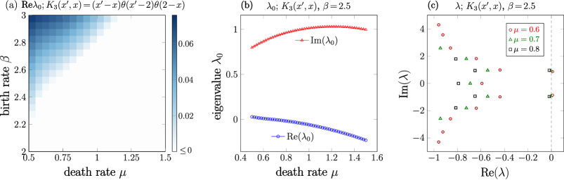
Figure 3: (a) Heatmap of the real part of the principle eigenvalue $\lambda_{0}$ associated with the Jacobian matrix of the discretized ODE system Eq. (15) at its fixed point. The top left region takes positive real values. (b) Dependence of the largest eigenvalue $\lambda_{0}$ on $\mu$ for $\beta=2.5$. When $\mu$ is small, $\text{Re}\lambda_{0}>0$, which indicates an unstable positive equilibrium. In (a) and (b), $\beta,\mu$ are age-independent, and the cannibalism rate is derived from $K_{3}$ in Eq. (12). (c) The first five eigenvalues for $\mu=0.6,0.7,0.8$ (open circle, triangle, square, respectively). When $\mu=0.6$, $\lambda_{0}$ has a positive real part; when $\mu=0.7,0.8$, $\lambda_{0}$ has a negative real part, implying stability of the steady state.

Generalizing to more compartments, if the Jacobian matrix ${\bf J}_{L}$ of the positive equilibrium $(n_{0}^{*},\ldots,n_{L}^{*})$ of the $(L+1)$-compartment reduced ODE model Eq. (15) has an unstable equilibrium, we can assume that

$$\textbf{v}_{L}\in\mathbb{R}^{L+1},\,\,{\bf J}_{L}\textbf{v}_{L}=\lambda\mathds{I}\textbf{v}_{L}=(v_{1},...,v_{L})\neq 0,\,\,\text{Re}\lambda>0.$$ (74)

For $L^{\prime}>L$, we can consider the following ODE model

$$\frac{\mathrm{d}n_{0}}{\mathrm{d}t}=-\mu_{0}(t)n_{0}(t)-n_{0}(t)\sum_{j=i}^{L}(K_{j,0}(t)n_{j}(t))+\sum_{j=1}^{L}\beta_{j}(t)n_{j}(t)-\frac{n_{0}(t)}{\Delta{x}},$$ (75)

$$\frac{\mathrm{d}n_{i}}{\mathrm{d}t}=-\mu_{i}(t)n_{i}(t)-n_{i}(t)\sum_{j=i}^{L}(K_{j,i}(t)n_{j}(t))-\frac{n_{i}(t)-n_{i-1}(t)}{\Delta{x}},\quad L\geq i>0,$$

$$\frac{\mathrm{d}n_{i}}{\mathrm{d}t}=\frac{n_{i-1}(t)-n_{i}(t)}{\Delta{x}},\quad\,\,i>L$$

which has a positive equilibrium $(n_{0}^{*},...,n_{L}^{*},n_{L+1}^{*},...,n_{L^{\prime}}^{*}),n_{i}^{*}=n_{L}^{*},i>L$. Denoting the Jacobian matrix of the equilibrium of the ODE Eq. (75) to be ${\bf J}_{L^{\prime}}$, it is obvious that $\lambda$ is also an eigenvalue of ${\bf J}_{L^{\prime}}$ with the corresponding eigenvector

$$\textbf{v}_{L^{\prime}}=(v_{1},...,v_{L},\tfrac{1}{1+\Delta{x}\lambda}v_{L},\dots,(\tfrac{1}{1+\Delta{x}\lambda})^{L^{\prime}-L}v_{L}).$$ (76)

Therefore, all reduced ODE systems with $L^{\prime}>L$ compartments have a positive equilibrium whose Jacobian matrix has a positive eigenvalue. Therefore, the positive equilibrium can be unstable, which could then lead to undamped oscillating solutions.

Appendix E Additional examples of overcompensation

E.1 Cannibalism-related birth rate

In the main discussion, we assumed that cannibalism only modifies the death rate. Here, we provide a numerical example in which preying on juveniles can increase birth rates. This limit may arise when food is not abundant and cannibalism provides nourishment for reproduction. We consider using the following coefficients in Eq. (5)

$$K(x^{\prime},x)=K_{1}(x^{\prime},x)\equiv\theta(x^{\prime}-2)\theta(2-x),\,\,\,\beta(x,\phi[n;x])=\beta_{0}+\frac{1}{4}\int_{0}^{\infty}K(x,x^{\prime})n(x^{\prime},t)\mathrm{d}{x^{\prime}},$$ (77)

where $\beta_{0},\mu$ are constants. We plot the total steady-state population at as a function of $\beta_{0}$ and $\mu$ in Fig. 4(b). When $\beta_{0}$ is fixed, the total population is found to first increase with the death rate $\mu$ until $\mu\rightarrow\beta_{0}^{+}$ when the population starts to diminish. This implies that for the cannibalism-rate-dependent birth rate $\beta$ defined in Eq. (77), overcompensation can arise.

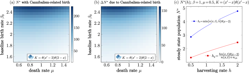
Figure 4: (a) The steady-state total population $N^{*}(\beta(x,\phi[n;x]))$ that displays overcompensation with a constant death rate for the cannibalism-dependent birth rate Eq. (77), where cannibalism has a positive effect on the birth rate. (b) The difference in the steady-state population $N^{*}(\beta(x,\phi[n;x]))-N^{*}(\beta_{0})$, where $N^{*}(\beta(x,t))$ is the steady-state total population with a constant birth rate $\beta\coloneqq\beta_{0}$. Because $\beta(x,\phi[n;x])>\beta_{0}$ for $n^{*}$, the difference is always positive. Furthermore, for some fixed $\beta_{0}$, the difference $N^{*}(\beta(x,\phi[n;x]))-N^{*}(\beta_{0})$ also “overcompensates” by first increase then decrease with $\mu\coloneqq\mu_{0}$. (c) The steady-state total population for $h_{1},h_{2}$ in Eq. (78) for the harvesting model Eq. (11). Overcompensation is observed with increasing harvesting rates. Furthermore, since $h_{1}>h_{2}$ if $h$ is the same, for a fixed $h$, the total population under the harvesting rate $h_{1}$ is greater than that under $h_{2}$.

E.2 Harvesting-induced overcompensation

Populations can also respond to age-dependent harvesting, as is practiced in animal culling and fisheries. Our age-structured Lotka-Volterra model can be modified to include a harvesting term $h(n;x,t)$ that could be a nonlinear function of $n$ (Diedrichs, 2019), as described by Eq. (11).

We explore age-dependent harvesting $h(n;x,t)$ that preferentially removes older populations and show numerically that overcompensation can arise for the two forms of harvesting

$$h_{1}=\min\{n(x,t),h\}\theta(x-2),\,\,\,h_{2}=\frac{hn(x,t)}{n(x,t)+n_{1/2}}\theta(x-2),$$ (78)

where $h$ is the intrinsic maximum harvesting rate and $n_{1/2}$ is a constant half-saturation density. Both effective harvesting rates $h_{1}$ and $h_{2}$ vanish with the population densities $n(x,t)$, saturate to $h$ when $n(x,t)\gg n_{1/2}$, and increase with the parameter $h$. We set all other dimensionless coefficients in Eq. (11) to $K(x^{\prime},x)=K_{4}(x^{\prime},x)=(x^{\prime}-x)\theta(x^{\prime}-x),\,\beta=1,\,\mu=0.5,\,n_{1/2}=1$. In Fig. (4)(a), we plot the plot steady-state population $N^{*}$ for scenarios $h_{1}$ and $h_{2}$ as a function of $h$. The total population $N^{*}$ is seen to increase with $h$ for both harvesting strategies, indicating overcompensation in response to increased harvesting rate.

E.3 Overcompensation following changes in birth rate

The usual “hydra effect” overcompensation is described by a steady state total population that increases with the death rate. In all of our examples, the total steady-state population increased with birth rate $\beta$. One can show that if $K(x^{\prime},x)\geq 0$ and $K(x^{\prime},x)=0$ for $x>X$ or $x^{\prime}\leq x$, the steady-state solutions to Eq. (7) that correspond to birth rates $\beta_{1}(x)>\beta_{2}(x)$, $n_{\beta_{1}}^{*}(x)$ and $n_{\beta_{2}}^{*}(x)$, are such that the total steady-state total populations

$$N^{*}_{\beta_{1}}\coloneqq\int_{0}^{\infty}\!n^{*}_{\beta_{1}}(x)\mathrm{d}{x}>N^{*}_{\beta_{2}}\coloneqq\int_{0}^{\infty}\!n^{*}_{\beta_{2}}(x)\mathrm{d}{x}.$$ (79)

In fact, steady-state solution $n^{*}(x),x\geq 0$ to Eq. (7) can be expressed in terms of $n^{*}(X)$

$$\left\{\begin{aligned} &n^{*}(x)=e^{-\int_{X}^{x}\mu(x^{\prime})\mathrm{d}{x^{\prime}}}\,n^{*}(X),\,\,\,x\geq X,\\ &n^{*}(x)=e^{\int_{x}^{X}\mu(x^{\prime})\mathrm{d}{x^{\prime}}}e^{\int_{x}^{X}\int_{x^{\prime}}^{\infty}\!K(y,x^{\prime})n^{*}(y)\mathrm{d}{y}\mathrm{d}{x^{\prime}}}\,n^{*}(X).\end{aligned}\right.$$ (80)

We conclude from Eq. (80) that if $n_{\beta_{1}}^{*}(X)>n_{\beta_{2}}^{*}(X)$ then $n_{\beta_{1}}^{*}(x)>n_{\beta_{2}}^{*}(x),x\geq 0$ and therefore Eq. (79) still holds.

On the other hand, if $n_{\beta_{1}}^{*}(X)\leq n_{\beta_{2}}^{*}(X)$, we conclude from Eq. (80) that $n_{\beta_{1}}^{*}(x)\leq n_{\beta_{2}}^{*}(x),x\geq 0$. However, from Eq. (42), we have

$$\int_{0}^{\infty}\!\beta_{i}(x)e^{-\int_{0}^{x}\tilde{\mu}_{i}(a)\mathrm{d}{a}}\mathrm{d}{x}=1,\,\,\,i=1,2$$ (81)

where

$$\tilde{\mu}_{1}(x)=\mu(x)+\int_{x}^{\infty}K(x^{\prime},x)n^{*}_{\beta_{1}}(x^{\prime})\mathrm{d}{x^{\prime}}\leq\tilde{\mu}_{2}(x)=\mu(x)+\int_{x}^{\infty}K(x^{\prime},x)n^{*}_{\beta_{2}}(x^{\prime})\mathrm{d}{x^{\prime}}.$$ (82)

Therefore,

$$1=\int_{0}^{\infty}\!\beta_{1}(x)e^{-\int_{0}^{x}\tilde{\mu}_{1}(a)\mathrm{d}{a}}\mathrm{d}{x}>\int_{0}^{\infty}\!\beta_{2}(x)e^{-\int_{0}^{x}\tilde{\mu}_{2}(a)\mathrm{d}{a}}\mathrm{d}{x}=1$$ (83)

is a contradiction implying $n_{\beta_{1}}^{*}(x)>n_{\beta_{2}}^{*}(x),x\geq 0$ and that the total steady-state population $n_{\beta_{1}}^{*}(x)>n_{\beta_{2}}^{*}(x),x\geq 0$ always increases with birth rate when $K\geq 0$ and the predation is unidirectional (old-eat-young).

In scenarios in which the younger population can prey on the older population, and $K$ can be negative, steady-state total populations can decrease with the birth rate, i.e., the steady-state total population “overcompensates” as the birth rate decreases. As an example, we assume a dimensionless predation rate of the form

$$\tilde{K}(x^{\prime},x)\equiv 2\theta(X-x^{\prime})-1,$$ (84)

set $X,\mu$, and $\beta$ to be dimensionless constants, and investigate how the population varies with $\beta$. Here, the young population $x^{\prime}<X$ suppresses the whole population as $\tilde{K}(x^{\prime},x)=1>0,\,x^{\prime}<X$, while the old population $x^{\prime}\geq X$ has a positive effect on the whole population since $\tilde{K}(x^{\prime},x)=-1,\,x^{\prime}\geq X$. The explicit solution for the steady-state population is

$$n^{*}(x)=\frac{\beta(\beta-\mu)e^{-\beta x}}{\big{(}1-2e^{-\beta X}\big{)}},\quad N^{*}=\!\int_{0}^{\infty}\!\!n^{*}(x)\mathrm{d}{x}=\frac{(\beta-\mu)}{\big{(}1-2e^{-\beta X}\big{)}}.$$ (85)

Upon taking the derivative $\partial_{\beta}N^{*}$, we find

$$\frac{\partial N^{*}}{\partial\beta}=\frac{1-2e^{-\beta X}-2(\beta-\mu)Xe^{-\beta X}}{\big{(}1-2e^{-\beta X}\big{)}^{2}},$$ (86)

and specifically, $\big{(}\partial N^{*}/\partial\beta\big{)}<0$ if $2+2(\beta-\mu)X>e^{\beta X}$. Therefore, if the interspecific interaction $K$ allows younger individuals to suppress the overall population, the steady-state population can overcompensate by decreasing as the birth rate $\beta$ is increased.

References

• Aarssen (1995) Aarssen, L.W., 1995. Hypotheses for the evolution of apical dominance in plants: implications for the interpretation of overcompensation. Oikos 74, 149–156.
• Abrams (2009) Abrams, P.A., 2009. When does greater mortality increase population size? The long history and diverse mechanisms underlying the hydra effect. Ecol. Lett. 12, 462–474.
• Boyce et al. (1999) Boyce, M.S., Sinclair, A., White, G.C., 1999. Seasonal compensation of predation and harvesting. Oikos 87, 419–426.
• Cantrell and Cosner (2001) Cantrell, R.S., Cosner, C., 2001. On the dynamics of predator–prey models with the Beddington–Deangelis functional response. Journal of Mathematical Analysis and Applications 257, 206–222.
• Chou and Greenman (2016) Chou, T., Greenman, C.D., 2016. A hierarchical kinetic theory of birth, death, and fission in age-structured interacting populations. Journal of Statistical Physics 164, 49–76.
• Chou et al. (2023) Chou, T., Shao, S., Xia, M., 2023. Adaptive hermite spectral methods in unbounded domains. Applied Numerical Mathematics 183, 201–220.
• Chuang et al. (2018) Chuang, Y.L., Chou, T., D’Orsogna, M.R., 2018. Age-structured social interactions enhance radicalization. Journal of Mathematical Sociology 42, 128–151.
• Cosner et al. (1999) Cosner, C., DeAngelis, D.L., Ault, J.S., Olson, D.B., 1999. Effects of spatial grouping on the functional response of predators. Theoretical population biology 56, 65–75.
• De Roos et al. (2007) De Roos, A., Schellekens, T., Van Kooten, T., Van De Wolfshaar, K., Claessen, D., Persson, L., 2007. Food-dependent growth leads to overcompensation in stage-specific biomass when mortality increases: the influence of maturation versus reproduction regulation. Am. Nat. 170, E59–E76.
• De Roos et al. (2008) De Roos, A., Schellekens, T., Van Kooten, T., Van De Wolfshaar, K., Claessen, D., Persson, L., 2008. Simplifying a physiologically structured population model to a stage-structured biomass model. Theor. Popul. Biol. 73, 47–62.
• Diedrichs (2019) Diedrichs, D.R., 2019. Using harvesting models to teach modeling with differential equations. PRIMUS 29, 712–723.
• Eymard et al. (2000) Eymard, R., Gallouët, T., Herbin, R., 2000. Finite volume methods. Handb. Numer. Anal. 7, 713–1018.
• Greenman and Chou (2016) Greenman, C.D., Chou, T., 2016. A kinetic theory of age-structured stochastic birth-death processes. Physical Review E 93, 2016.
• Grenfell et al. (1992) Grenfell, B.T., Price, O.F., Albon, S.D., Glutton-Brock, T.H., 1992. Overcompensation and population cycles in an ungulate. Nature 355, 823–826.
• Grosholz et al. (2021) Grosholz, E., Ashton, G., Bradley, M., Brown, C., Ceballos-Osuna, L., Chang, A., Rivera, C., Gonzalex, J., Heineke, M., Marraffini, M., McCann, L., Pollard, E., Pritchard, I., Ruiz, G., Turner, B., Pepolt, C., 2021. Stage-specific overcompensation, the hydra effect, and the failure to eradicate an invasive predator. P. Natl. A. Sci. 118.
• Keyfitz and Keyfitz (1997) Keyfitz, B.L., Keyfitz, N., 1997. The McKendrick partial differential equation and its uses in epidemiology and population study. Math. Comput. Model. 26, 1–9. URL: https://doi.org/10.1016/S0895-7177(97)00165-9.
• Kozlov et al. (2017) Kozlov, V., Radosavljevic, S., Wennergren, U., 2017. Large time behavior of the logistic age-structured population model in a changing environment. Asymptotic Ana. 102, 21–54.
• Lennartsson et al. (2018) Lennartsson, T., Ramula, S., Tuomi, J., 2018. Growing competitive or tolerant? Significance of apical dominance in the overcompensating herb Gentianella campestris. Ecology 99, 259–269.
• Liu and Cohen (1987) Liu, L., Cohen, J.E., 1987. Equilibrium and local stability in a logistic matrix model for age-structured populations. J. Math. Biol. 25, 73–88.
• Liz and Ruiz-Herrera (2012) Liz, E., Ruiz-Herrera, A., 2012. The hydra effect, bubbles, and chaos in a simple discrete population model with constant effort harvesting. J. Math. Biol. 65, 997–1016.
• Liz and Ruiz-Herrera (2022) Liz, E., Ruiz-Herrera, A., 2022. Stability, bifurcations and hydra effects in a stage-structured population model with threshold harvesting. Commun. Nonlinear Sci. 109, 106280.
• Lotka (2002) Lotka, A.J., 2002. Contribution to the theory of periodic reactions. J. Phys. Chem. 14, 271–274.
• McIntire and Juliano (2018) McIntire, K.M., Juliano, S.A., 2018. How can mortality increase population size? a test of two mechanistic hypotheses. Ecology 99, 1660–1670.
• Ohba et al. (2006) Ohba, S., Hidaka, K., Sasaki, M., 2006. Notes on paternal care and sibling cannibalism in the giant water bug, Lethocerus deyrolli (heteroptera: Belostomatidae). Entomological Science 9, 1–5.
• Ohlberger et al. (2011) Ohlberger, J., Langangen, Ø., Edeline, E., Claessen, D., Winfield, I.J., Stenseth, N.C., VØllestad, L.A., 2011. Stage-specific biomass overcompensation by juveniles in response to increased adult mortality in a wild fish population. Ecology 92, 2175–2182.
• Pachepsky et al. (2008) Pachepsky, E., Nisbet, R.M., Murdoch, W.W., 2008. Between discrete and continuous: consumer–resource dynamics with synchronized reproduction. Ecology 89, 280–288.
• Schröder et al. (2014) Schröder, A., van Leeuwen, A., Cameron, T.C., 2014. When less is more: positive population-level effects of mortality. Trend. Ecol. Evol. 29, 614–624.
• Sharpe and Lotka (1911) Sharpe, F.R., Lotka, A.J., 1911. A problem in age-distribution. The London, Edinburgh, and Dublin Philosophical Magazine and Journal of Science 21, 435–438. URL: https://doi.org/10.1080/14786440408637050.
• Sorenson and Cortez (2021) Sorenson, D.K., Cortez, M.H., 2021. How intra-stage and inter-stage competition affect overcompensation in density and hydra effects in single-species, stage-structured models. Theor. Ecol.-Neth. 14, 23–39.
• Thomas and Manica (2003) Thomas, L.K., Manica, A., 2003. Filial cannibalism in an assassin bug. Animal Behaviour 66, 205–210.
• Volterra (1928) Volterra, V., 1928. Variations and fluctuations of the number of individuals in animal species living together. ICES J. Mar. Sci. 3, 3–51.
• Wikan and Kristensen (2021) Wikan, A., Kristensen, Ø., 2021. Compensatory and overcompensatory dynamics in prey–predator systems exposed to harvest. Journal of Applied Mathematics and Computing 67, 455–479.
• Wise and Abrahamson (2005) Wise, M.J., Abrahamson, W.G., 2005. Beyond the compensatory continuum: environmental resource levels and plant tolerance of herbivory. Oikos 109, 417–428.
• Wise and Abrahamson (2008) Wise, M.J., Abrahamson, W.G., 2008. Applying the limiting resource model to plant tolerance of apical meristem damage. Am. Nat. 172, 635–647.
• Xia and Chou (2021) Xia, M., Chou, T., 2021. Kinetic theory for structured population models: application to stochastic sizer-timer models of cell proliferation. Journal of Physics A 54, 385601.
• Xia et al. (2021a) Xia, M., Shao, S., Chou, T., 2021a. Efficient scaling and moving techniques for spectral methods in unbounded domains. SIAM J. Sci. Comput. 43, A3244–A3268.
• Xia et al. (2021b) Xia, M., Shao, S., Chou, T., 2021b. A frequency-dependent p-adaptive technique for spectral methods. J. Comput. Phys. 446, 110627.