Parallel and Distributed Exact Single-Source Shortest Paths with Negative Edge Weights

Abstract

This paper presents parallel and distributed algorithms for single-source shortest paths when edges can have negative weights (negative-weight SSSP). We show a framework that reduces negative-weight SSSP in either setting to $n^{o(1)}$ calls to any SSSP algorithm that works with a virtual source. More specifically, for a graph with $m$ edges, $n$ vertices, undirected hop-diameter $D$, and polynomially bounded integer edge weights, we show randomized algorithms for negative-weight SSSP with

• $W_{SSSP}(m,n)n^{o(1)}$ work and $S_{SSSP}(m,n)n^{o(1)}$ span, given access to an SSSP algorithm with $W_{SSSP}(m,n)$ work and $S_{SSSP}(m,n)$ span in the parallel model, and

• $T_{SSSP}(n,D)n^{o(1)}$, given access to an SSSP algorithm that takes $T_{SSSP}(n,D)$ rounds in $\mathsf{CONGEST}$.

This work builds off the recent result of Bernstein, Nanongkai, Wulff-Nilsen Bernstein et al. (2022), which gives a near-linear time algorithm for negative-weight SSSP in the sequential setting.

Using current state-of-the-art SSSP algorithms yields randomized algorithms for negative-weight SSSP with

• $m^{1+o(1)}$ work and $n^{1/2+o(1)}$ span in the parallel model, and

• $(n^{2/5}D^{2/5}+\sqrt{n}+D)n^{o(1)}$ rounds in $\mathsf{CONGEST}$.

Up to a $n^{o(1)}$ factor, these match the current best upper bounds for reachability Jambulapati et al. (2019); Cao et al. (2021). Consequently, any improvement to negative-weight SSSP in these models beyond the $n^{o(1)}$ factor necessitates an improvement to the current best bounds for reachability.

Our main technical contribution is an efficient reduction for computing a low-diameter decomposition (LDD) of directed graphs to computations of SSSP with a virtual source. Efficiently computing an LDD has heretofore only been known for undirected graphs in both the parallel and distributed models. The LDD is a crucial step of the algorithm in Bernstein et al. (2022), and we think that its applications to other problems in parallel and distributed models are far from being exhausted.

Other ingredients to our results include altering the recursion structure of the scaling algorithm in Bernstein et al. (2022) to surmount difficulties that arise in parallel and distributed models, and also an efficient reduction for computing strongly connected components to computations of SSSP with a virtual source in $\mathsf{CONGEST}$. The latter result answers a question posed in Bernstein and Nanongkai (2019) in the negative.

1 Introduction

Single-source shortest paths (SSSP) is one one the most fundamental algorithmic graph problems there is. Given a directed graph $G=(V,E)$, an integer weight function $w:E\rightarrow\mathbb{Z}$, and a source vertex $s\in V$, we want to compute the distance from $s$ to $v$ for all $v\in V$.

Efficient solutions to this problem are typically better understood in the regime where edge weights are non-negative. Dijkstra’s algorithm, from the 50s, is one such solution which runs in near-linear time but whose correctness holds under the restriction that inputs have non-negative edge weights. The picture for single-source shortest paths with negative weights (negative-weight SSSP) in the sequential setting, on the other hand, has up to very recently been a work in progress towards finding a near-linear time algorithm. From the 50s, the classic Bellman-Ford algorithm gives an $O(mn)$ time algorithm which either computes distances from $s$ to $v$ or reports a negative-weight cycle. Goldberg’s algorithm Goldberg (1995), from the 90s, achieves a runtime of $\widetilde{O}(m\sqrt{n})$ using a scaling technique. Slightly more recently, there have been several other algorithms Cohen et al. (2017); van den Brand et al. (2020); Axiotis et al. (2020) for the more general problems of transshipment and min-cost flow using sophisticated continuous-optimization methods, implying an algorithm for negative-weight SSSP that runs in near-linear time on moderately dense graphs. It is only within the last year that the major breakthrough by Chen, Kyng, Liu, Peng, Probst Gutenberg, and Sachdeva Chen et al. (2022), using continuous-optimization methods, culminated this series of works, which thus implies an $O(m^{1+o(1)})$ time algorithm for negative-weight SSSP. In a parallel and independent work, Bernstein, Nanongkai, Wulff-Nilsen Bernstein et al. (2022) gave a $\widetilde{O}\mathopen{}\mathclose{{}\left(m}\right)$ time algorithm for negative-weight SSSP that uses relatively simpler techniques. In this paper, we take the exploration of negative-weight SSSP to parallel and distributed models of computation. Should there be analogous results there?

In parallel models, much progress has been made with SSSP algorithms. Very recently, Rozhoň, Haeupler, Martinsson, Grunau and Zuzic Rozhoň et al. (2022) and Cao and Fineman Cao and Fineman (2023) show that SSSP with polynomially bounded non-negative integer edge weights can be solved with $\widetilde{O}(m)$ work and $n^{1/2+o(1)}$ depth in the parallel model. In contrast, the Bellman-Ford algorithm solves negative-weight SSSP with $O(mn)$ work and $O(n)$ depth. Cao, Fineman and Russell Cao et al. (2022) proposed an algorithm solving negative-weight SSSP with $\widetilde{O}(m\sqrt{n})$ work and $n^{5/4+o(1)}$ depth.

Similarly, in distributed models, Rozhoň et al. Rozhoň et al. (2022) and Cao and Fineman Cao and Fineman (2023) show algorithms for SSSP with non-negative integer edge weights that take $\widetilde{O}((n^{2/5+o(1)}D^{2/5}+\sqrt{n}+D)$ rounds. On the negative-weight SSSP front, the Bellman-Ford algorithm takes $O(n)$ rounds. The current state-of-the-art by Forster, Goranci, Liu, Peng, Sun and Ye Forster et al. (2022), which uses Laplacian solvers, gives an $\widetilde{O}(m^{3/7+o(1)}(n^{1/2}D^{1/4}+D))$ round algorithm for negative-weight SSSP.

There is a substantial gap between the best known upper bounds for SSSP and negative-weight SSSP in these models and, in fact, the number of landmark algorithms for negative-weight SSSP have been comparatively few. This begets the following question: Can we close the gap, and get parallel and distributed algorithms for negative-weight SSSP that are nearly as efficient as the best SSSP algorithms? This paper gives an answer in the affirmative. The main results of this paper are as follows.

Theorem 1.1 (Parallel negative-weight SSSP, proved in Section 7).

There is a randomized parallel algorithm that, given an n-node m-edge directed graph with polynomially bounded integer edge weights, solves the exact single-source shortest path problem with $m^{1+o(1)}$ work and $n^{1/2+o(1)}$ span, with high probability.

Theorem 1.2 (Distributed negative-weight SSSP, proved in Section 8.3).

There is a distributed randomized algorithm that, given an $m$-edge $n$-node directed graph with polynomially bounded integer edge weights and undirected hop-diameter $D$, solves the exact single source shortest path problem with $O((n^{2/5+o(1)}D^{2/5}+\sqrt{n}+D)n^{o(1)})$ rounds of communication in the $\mathsf{CONGEST}$ model with high probability.

A Research Agenda for Basic Algorithms

Bernstein et al. Bernstein et al. (2022) poses a research agenda of designing simple (combinatorial) algorithms for fundamental graph problems, to catch up to the extent possible with algorithms that rely on min-cost flow, whose state-of-the-art involves sophisticated methods from continuous optimization. One of the main attractions of this line of research is the belief that simple algorithms are more amenable to being ported across to different well-studied models of computation. Our results provide support to this belief by giving an analog of the simple negative-weight SSSP algorithm in parallel and $\mathsf{CONGEST}$ models.

1.1 Our Contributions

On top of algorithms for negative-weight SSSP, we provide several algorithms that may be of independent interest, such as an efficient low-diameter decomposition for directed graphs, and computing strongly connected components in distributed models of computation. These algorithms, and the algorithms that directly address negative-weight SSSP, are actually general reductions to SSSP (this includes Theorems 1.1 and 1.2 among others). One advantage of this approach is that our results scale with SSSP; if there is any progress in the upper bounds to SSSP, progress to the bounds in this paper immediately follow.

We first give the definition of the SSSP oracle that we make reductions to.

Definition 1.3 ($(dist_{G}(s,v))_{v\in V}\leftarrow\mathcal{O}^{NN-SSSP}(G=(V,E,w),s)$).

The non-negative single source shortest path oracle $\mathcal{O}^{NN-SSSP}$ takes inputs (i) A directed graph $G=(V,E,w)$ with non-negative polynomially bounded integer edge weights (ii) A vertex $s\in V$, and returns the distance from $s$ to all vertices in $V$.

Now, we provide the statement for the reduction from low-diameter decomposition to oracle $\mathcal{O}^{NN-SSSP}(G,s)$ (for more details, see Section 4).

Low Diameter Decomposition

Lemma 1.4 (Low-Diameter Decomposition, Algorithm 1).

Let $G=(V,E,w)$ be a directed graph with a polynomially bounded weight function $w:E\to\mathbb{N}$ and let $d$ be a positive integer. There exists a randomized algorithm $LowDiameterDecomposition(G,d)$ with following guarantees:

• INPUT: an $n$-node $m$-edge, graph $G=(V,E,w)$ with non-negative integer edge weight and a positive integer $d$.

• OUTPUT: (proved in Section 4.2) a set of edges $E^{rem}\subseteq E$ satisfying:

  • each SCC of the subgraph $E-E^{rem}$ has weak diameter at most $d$ in $G$, i.e. if $u,v$ are two vertices in the same SCC, then $dist_{G}(u,v)\leq d$ and $dist_{G}(v,u)\leq d$.

  • for any $e\in E$, we have $\mathbf{Pr}[e\in E^{rem}]=O\mathopen{}\mathclose{{}\left(\frac{w(e)\log^{2}n}{d}+\frac{1}{n^{8}}}\right)$

• RUNNING TIME: The algorithm is randomized and takes $\widetilde{O}(1)$ calls to $\mathcal{O}^{NN-SSSP}$. More specifically,

  • (Proved in Section 7) assuming there is a parallel algorithm answering $\mathcal{O}^{NN-SSSP}$ in $W(m,n)$ work and $S(m,n)$ span, then $LowDiameterDecomposition(G,d)$ takes $\widetilde{O}(W(m,n))$ work and $\widetilde{O}(S(m,n))$ span with high probability.

  • (Proved in Section 8.2) assuming there exists a $\mathsf{CONGEST}$ algorithm answering $\mathcal{O}^{NN-SSSP}_{S}$ in $T(n,D)$ rounds, then $LowDiameterDecomposition(G,d)$ takes $\widetilde{O}(T(n,D)+\sqrt{n}+D)$ rounds in the $\mathsf{CONGEST}$ model with high probability, where $D$ is the undirected hop diameter.

Remark

In the $\mathsf{CONGEST}$ model, we are using $\mathcal{O}^{NN-SSSP}_{S}$ instead of $\mathcal{O}^{NN-SSSP}$. The main difference is that $\mathcal{O}^{NN-SSSP}_{S}$ allows querying graph with virtual super source. See 8.3 for the precise definition.

This result forms the basis for our improved SSSP algorithms. Using the parallel low-diameter decomposition, we argue that careful modification of the algorithmic and analytic insights of Bernstein et al.’s algorithm Bernstein et al. (2022) suffices to obtain improvements for a parallel negative-weight SSSP algorithm.

Theorem 1.5 (Parallel SSSP reduction with negative edge-weight, proved in Section 7).

Assuming there is a parallel algorithm answering SSSP oracle $\mathcal{O}^{NN-SSSP}$ in $W(m,n)$ work and $S(m,n)$ span, then exists a randomized algorithm that solves single-source shortest-paths problem for directed $n$-node graph $G$ with polynomially bounded integer edge-weight with $O(W(m,n)(\log n)^{O(\sqrt{\log n})})$ work and $\widetilde{O}(S(m,n)2^{\sqrt{\log n}})$ span with high probability.

We also prove an analogous result in the $\mathsf{CONGEST}$ model.

Theorem 1.6 (Distributed SSSP reduction with negative edge-weight, proved in Section 8.3).

In the $\mathsf{CONGEST}$ model, assuming there is an algorithm answering SSSP oracle $\mathcal{O}^{NN-SSSP}_{S}$ in $T(n,D)$ rounds, then there exists a randomized algorithm that solves single-source shortest-paths problem for directed $n$-node graph $G$ with polynomially bounded integer edge-weights and undirected hop-diameter $D$ in $O((T(n,D)+\sqrt{n}+D)(\log n)^{O(\sqrt{\log n})})$ rounds with high probability.

Theorems 1.5 and 1.6 give us reductions from SSSP with negative integer edge-weights to SSSP with non-negative integer edge-weight in the parallel and distributed model. Using the-state-of-art non-negative SSSP (Rozhoň et al. (2022) and Cao and Fineman (2023)) immediately gives Theorems 1.1 and 1.2.

SCC+Topsort

Our result for finding strongly connected components in the $\mathsf{CONGEST}$ model is as follows.

[Reduction for SCC+Topsort in $\mathsf{CONGEST}$ ]lemmascctopcongest There is a $\mathsf{CONGEST}$ algorithm that, given a directed graph $G=(V,E)$, and assuming there is an algorithm answering SSSP oracle $\mathcal{O}^{NN-SSSP}_{S}$ in $T(n,D)$ rounds, outputs SCCs in topological order. More specifically, it outputs a polynomially-bounded labelling $(r_{v})_{v\in V}$ such that, with high probability

1. $r_{u}=r_{v}$ if and only if $u$ and $v$ are in the same strongly connected component;

2. when the SCC that $u$ belongs to has an edge towards the SCC that $v$ belongs to, $r_{u}>r_{v}$.

The algorithm takes $\widetilde{O}\mathopen{}\mathclose{{}\left(T(n,D)+\sqrt{n}+D}\right)$ rounds.

It is worth noting that a more careful examination gives a round complexity in terms of calls to a reachability oracle, rather than an SSSP oracle. Incidentally, instantiating the oracle with the current state-of-the-art SSSP algorithm (Rozhoň et al. (2022) and Cao and Fineman (2023)) leads to a $\widetilde{O}\mathopen{}\mathclose{{}\left(n^{1/2}+D+n^{2/5+o(1)}D^{2/5}}\right)$ round algorithm (Corollary 9.4), answering a question posed in Bernstein and Nanongkai (2019) which asked if a lower bound of $\widetilde{\Omega}\mathopen{}\mathclose{{}\left(n}\right)$ rounds applies to the problem of finding SCCs. More on both points in Section 9.

Technique Overview

Broadly speaking, we port the algorithm of Bernstein et al. (2022) into parallel and distributed models of computation. The main difficulties in this are: (i) There being no known efficient algorithm for computing an LDD in parallel and distributed models. The algorithm in Bernstein et al. (2022) is fundamentally sequential, and it is not clear how to sidestep this. (ii) It being unclear how the algorithm in Bernstein et al. (2022) without using Dijkstra’s algorithm. (iii) There being no efficient $\mathsf{CONGEST}$ algorithm for finding strongly connected components of a DAG in topological order. We go into each point, in more detail, in Section 2.

1.2 Organization

Section 2 contains a high-level overview of our results, which explain the key difficulties of bringing over the result of Bernstein et al. (2022) to parallel and distributed models, and some intuition for how these are overcome. Section 3 covers terminology, notation, and some basic results we use; this may be skipped and returned to as and when necessary. For details on the low-diameter decomposition reduction, Section 4 covers the main ideas and Section 11 contains some of the omitted proofs. For details on the negative-weight SSSP algorithm reduction, Section 5 covers the general framework, Section 6 in the appendix contains the key technical details, while Sections 10 and 12 in the appendix contain details and proofs related to simpler subroutines. For an implementation of either the low-diameter decomposition or the negative-weight SSSP algorithm in the parallel or $\mathsf{CONGEST}$ model, see Sections 7 and 8. Finally, for details on finding strongly connected components in $\mathsf{CONGEST}$, along with a topological ordering of the components, see Section 9.

2 High Level Overview

Our results follow the framework of Bernstein et al. (2022), which provides a sequential algorithm for negative-weight SSSP that takes $\widetilde{O}(m)$ time with high probability (and in expectation). The core difficulty in bringing the sequential algorithm there to parallel and distributed models of computation lies in the scaling subroutine ScaleDown, which we focus most of the efforts in this work towards. In this section, we summarize ScaleDown and highlight the key areas of difficulty.

2.1 The Scaling Subroutine of Bernstein et al. (2022)

The input to ScaleDown is a weighted directed graph whose weights are no lower than $-2B$, for some non-negative $B$. The output of ScaleDown is a price function over vertices under which the weights of edges are no lower than $-B$. The price function ScaleDown computes is the distance from a virtual source $s$ to every vertex $v$ on $G^{B}$, which is $G$ with all negative-weight edges raised by $B$. Thus for much of ScaleDown we will be thinking about how to make the edges of $G^{B}$ non-negative without changing its shortest path structure. ScaleDown consists of four phases.

• Phase 0: Run a Low Diameter Decomposition on $G^{B}$ with negative-weight edges rounded up to $0$. This gives a set $E^{rem}$ of removed edges, and partitions the vertex set into strongly connected components (SCCs) that can be topologically ordered after having removed $E^{rem}$.

• Phase 1: Recursively call ScaleDown on the edges inside each SCC. This finds a price function on vertices under which edges inside each SCC have non-negative weight, thus fixing them.

• Phase 2: Fix DAG edges (i.e. the edges not in $E^{rem}$, that connect one component to another).

• Phase 3: Run epochs of Dijkstra’s Algorithm with Bellman-Ford iterations to fix the remaining negative-weight edges, all of which are contained in $E^{rem}$.

Observe that between Phases 1 to 3, all the edges are fixed. That is, the weight of edges in $G^{B}$ are non-negative, and consequently the weights of edges in $G$ are at least $-B$.

The key obstacles to porting ScaleDown to parallel and distributed models are as follows.

Obstacle 1: Low Diameter Decomposition

The work of Bernstein et al. Bernstein et al. (2022) gives a sequential algorithm solving directed LDD in $\widetilde{O}\mathopen{}\mathclose{{}\left(m}\right)$ time. Their algorithm runs in a recursive manner, described as follows.

• (Phase I) Categorize vertices as heavy or light. Heavy vertices have mutual distances $O(d)$ and we can ignore them; a light vertex has a small number of vertices with distance $O(d)$ to it.

• (Phase II) Sequentially carve out balls with a light vertex as center and with random radius (follows geometric distribution with mean value roughly $d$) where each ball becomes a recursive instance and the edges on the ball’s boundary are added to $E^{rem}$.

The key property to bound recursive depth is that each ball has size at most $.9|V|$ since the center is light. Finally, the algorithm recursively solves induced subgraphs $G[V_{i}]$ for each subset $V_{i}$ and adds the result to $E^{rem}$. Phase II is a highly sequential procedure that cannot be adapted to the parallel or $\mathsf{CONGEST}$ model efficiently, since the number of balls can be as large as $\Theta(n)$ for small $d$, which is considered a bad running time in both models. This is due to the fact that each ball only has its size upper bounded by $.9|V|$, but not lower bounded.

To this end, we take a different approach. Instead of simply carving out balls one by one where each ball only has size upper bounded by $.9|V|$ but lower bounded by nothing, we use a designated subroutine (Algorithm 2) to find a set $A\subseteq V$ such that $.1|V|\leq|A|\leq.9|V|$. $A$ is not necessarily a ball anymore, but a union of balls. It is also guaranteed that an edge is included in $A$’s boundary with small probability. In this way, we can recurse on two sets $A,V\backslash A$ thus avoiding inefficient computations.

Obstacle 2: From Dijkstra’s Algorithm to Oracles

By Phase 3 in Bernstein et al. (2022), the only remaining negative edges, which are all contained in $E^{rem}$, are fixed by computing distances from a dummy source $s$. While it seems like we are trying to solve negative-weight SSSP all over again, we can make use of the fact that $|E^{rem}|$ and thus the number of negative edges will be small in expectation. In particular, Bernstein et al. (2022) presents the algorithm ElimNeg with running time $O(m\widehat{\eta})$, where $\widehat{\eta}$ is the average number (over $v\in V$) of negative edges on a shortest path from $s$ to $v$. The LDD of Phase 0 guarantees that $\widehat{\eta}$ is polylogarithmic in $n$, hence ElimNeg is efficient in the sequential setting.

It is unclear how ElimNeg can be ported over to parallel and distributed models. In the sequential setting, ElimNeg runs multiple epochs where each epoch is, loosely speaking, an execution of Dijkstra’s algorithm followed by one iteration of the Bellman-Ford algorithm where, crucially, each execution of Dijkstra’s algorithm does not pay for the whole graph. ElimNeg guarantees that there is no more computation involving vertices $v$ after the first $\eta(v)$ epochs, where $\eta(v)$ is the number of negative edges on a shortest path from $s$ to $v$. It then follows, roughly, that there are $O(\sum_{v\in V}\eta(v))=O(m\widehat{\eta})$ computations.

In parallel and distributed models, however, it is not clear how to ensure that $v$ is involved in at most $\eta(v)$ computations. Even more, Dijkstra’s algorithm has the nice property that only vertices whose distances have been updated are involved in computation. It is unclear how an SSSP oracle, a blackbox that replaces Dijkstra’s algorithm, can be executed in a way that does not pay for the whole graph each time it is called. We end up settling for a weaker algorithm than ElimNeg, where each SSSP oracle call pays for the whole graph. Naively, this results in $O(\max_{v}\eta(v))$ calls to the oracle which is much too inefficient. While the LDD guarantees that $\eta(v)$ is polylogarithmic in expectation for all $v$, this does not hold with high probability; the maximum $\eta(v)$ could be as high as $\sqrt{n}$, resulting in $\sqrt{n}$ calls (as opposed to $n^{o(1)}$ calls) to the SSSP oracle. We instead truncate the number of calls to $n^{o(1)}$; in this way, we compute a distance estimate for every vertex: if the shortest path from $s$ to $v$ has at most $n^{o(1)}$ negative edges, we have the true distance in our hands, and otherwise we have the distance of a shortest path using no more than $n^{o(1)}$ negative edges which is an overestimation.

To resolve this and turn our estimates into true distances, we run $O(\log n)$ independent copies of LDD (more specifically, Phases 0 to 3). With high probability at least one of these estimates coincides with the true distance, which is what we want. Computing the indpendent LDDs changes the recursion structure of Scaledown, where we go from $O(\log n)$ invocations of linear recursion (see Figure 1) to $O(\log n)^{O(\sqrt{\log n})}=n^{o(1)}$ invocations of tree recursion (see Figure 2).

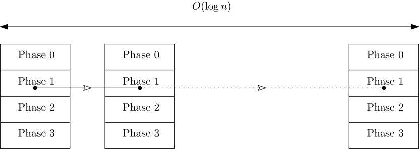
Figure 1: Recursion structure of ScaleDown in Bernstein et al. (2022).

Figure 2: Recursion structure of ScaleDown in this paper.

We note that this change in both the recursion structure and the parameters used to support it is the key reason for the $n^{o(1)}$ overhead over SSSP, and it is an interesting open question to reduce this overhead to $\textrm{polylog}(n)$.

Obstacle 3: SCC + Topological Sort in $\mathsf{CONGEST}$.

The framework of Schudy Schudy (2008) gives us an algorithm for SCC+Topsort in parallel models that uses $O(\log^{2}n)$ calls to $\mathcal{O}^{NN-SSSP}$ and yet, somewhat surprisingly, there has been no such algorithm formally written for $\mathsf{CONGEST}$.

Some care needs to be taken with bringing this idea into $\mathsf{CONGEST}$. Namely, how can recursive calls be orchestrated so as to achieve an efficient round complexity? The algorithm recurses into induced subgraphs, which may have a much larger undirected hop-diameter than the base graph; naively making calls to $\mathcal{O}^{NN-SSSP}$ on recursive instances consequently yields an inefficient distributed algorithm. Nevertheless, with some work done , this idea can be brought into $\mathsf{CONGEST}$.

We show how to overcome the above obstacles by using the Distributed Minor-Aggregation Model (see Section 8), which is an abstraction that affords us a relatively detail-free description of SCC+Topsort, avoiding much of the low level work hinted at above. For further details, see Section 9.

3 Definitions and Preliminaries

A weighted directed graph $G$ is a triple $(V,E,w)$ where $w:E\rightarrow R$ is a weight function. For a weighted directed graph $G$, the number of vertices and edges are $|V(G)|=n$ and $|E(G)|=m$, respectively. We denote the set of negative edge by $E^{neg}(G)=\{e\in E\mid w(e)<0\}$. For a subset $V^{\prime}\subset V$, we denote the induced graph on $V^{\prime}$ by $G[V^{\prime}]$ and the induced edges on $V^{\prime}$ by $E(V^{\prime})$. For an edge set $E^{\prime}\subseteq E$, when we treat $E^{\prime}$ as a subgraph of $G$, we mean the graph $(\{u,v\mid(u,v)\in E^{\prime}\},E^{\prime},w)$. A path is a sequence of vertices joined by edges; sometimes we refer to the path by the sequence of vertices and sometimes by the edges, depending on what is more convenient.

For a path $\Gamma=\langle v_{0},v_{1},\ldots,v_{k}\rangle$, the weight of $\Gamma$ is given by $w(\Gamma)=\sum_{i=1}^{k}w(v_{i-1},v_{i})$, that is, the sum of the weights of the edges on the path. For a pair of nodes $u,v\in V$, the shortest path distance from $u$ to $v$ is the minimum length over all paths that start at $u$ and end at $v$. We use $\mathit{dist}_{G}(u,v)$ to denote this shortest path distance with respect to the graph $G$. When the graph $G$ is clear in the context, we simply write $\mathit{dist}(u,v)$. If there is no $u$-to-$v$ path, then we define $\mathit{dist}(u,v)=+\infty$. Given a directed graph $G=(V,E,w)$, a vertex $s\in V$ and $d\in\mathbb{N}$, we define $\operatorname{Ball_{G}^{in}}(s,d)=\{v\mid dist_{G}(v,s)\leq d\}$ and $\operatorname{Ball_{G}^{out}}(s,d)=\{v\mid dist_{G}(s,v)\leq d\}$ be the ball within distance $d$. For a given graph $G=(V,E,w)$ set $S\subseteq V$, we define $\delta^{-}(S)=\{(u,v)\in E\mid u\not\in S,v\in S\}$ and $\delta^{+}(S)=\{(u,v)\in E\mid u\in S,v\not\in S\}$ be the edge set Crossing $S$ .

When we say that an algorithm achieves some performance $O(f(n))$ with high probability, we mean the following: for any particular choice of constant $c>0$, with probability at least $1-1/n^{c}$ the algorithm achieves performance $O(f(n))$.

Dependence on $W_{in}$

Throughout the paper, we will assume the maximum weight edge (in absolute value), $W_{in}$, is polynomially bounded and ignore the $\log W_{in}$ term throughout the paper. Based on the following theorem, we only have one $\log W_{in}$ factor. The proof is deferred to section 12.

Theorem 3.1.

In the distributed or parallel model, if there is an algorithm solving exact SSSP with polynomially bounded negative integer edge weight with runtime $T(m,n)$(work, span, or rounds), then there exists an algorithm solving exact SSSP with edge weight from $\{-W_{in},-(W_{in}-1),...,0,1,...,W_{in}-1,W_{in}\}$ with runtime $\widetilde{O}(T(m,n)\log W_{in})$.

$\mathsf{CONGEST}$ model.

Suppose the communication happens in the network $G=(V,E)$. In the $\mathsf{CONGEST}$ model, time is divided into discrete time slots, where each slot is called a round. Throughout the paper, we always use $n$ to denote the number of vertices in our distributed network, i.e., $|V|$. In each round, each vertex in $V$ can send an $O(\log n)$ bit message to each of its neighbors. At the end of each round, vertices can do arbitrary local computations. A $\mathsf{CONGEST}$ algorithm initially specifies the input for each vertex, after several rounds, all vertices terminate and generate output. The time complexity of a $\mathsf{CONGEST}$ algorithm is measured by the number of rounds.

Distributed inputs and outputs.

Since the inputs and outputs to the distributed network should be specified for each vertex, we must be careful when we say something is given as input or output. Here we make some assumptions. For the network $G=(V,E)$, we say a subset of vertices (or a single vertex) $V^{\prime}\subseteq V$ is the input or output if every vertex is given the information about whether it is in $V^{\prime}$. We say a subgraph $H$ (a subset of edges, for example, paths or circles) is the input or output if every vertex knows the edges in $H$ adjacent to it. We say a number is an input or output, we normally mean the number is the input or output of every vertex unless otherwise specified.

Distributed directed single source shortest path problem.

In this problem, each edge $e$ in the network $G=(V,E)$ is assigned an integer weight $w(e)$ and a direction, which defines a weighted directed graph $G^{\prime}=(V,E,w)$. A source node $s$ is specified. In $\mathsf{CONGEST}$ model, the inputs are (i) each node knows the weights and directions of all its incident edges, (ii) each node knows whether it is $s$ or not. The goal is to let every node $v$ output $dist_{G^{\prime}}(s,v)$.

3.1 Definitions from Bernstein et al. (2022).

The following two definitions are taken from Bernstein et al. (2022) and are heavily used in Section 6.

Definition 3.2 ($G_{s},w_{s},G^{B},w^{B},G^{B}_{s},w^{B}_{s}$).

[Definition 2.3 of Bernstein et al. (2022)]

Given any graph $G=(V,E,w)$, we let $G_{s}=(V\cup\{s\},E\cup\{(s,v)\colon v\in V\},w_{s})$ refer to the graph $G$ with a dummy source $s$ added, where there is an edge of weight $0$ from $s$ to $v$ for every $v\in V$ and no edges into $s$. Note that $G_{s}$ has a negative-weight cycle if and only if $G$ does and that $dist_{G_{s}}(s,v)=\min_{u\in V}dist_{G}(u,v)$.
For any integer $B$, let $G^{B}=(V,E,w^{B})$ denote the graph obtained by adding $B$ to all negative edge weights in $G$, i.e., $w^{B}(e)=w(e)+B$ for all $e\in E^{neg}(G)$ and $w^{B}(e)=w(e)$ for $e\in E\setminus E^{neg}(G)$. Note that $(G^{B})_{s}=(G_{s})^{B}$ so we can simply write $G^{B}_{s}=(V\cup\{s\},E\cup\{(s,v)\colon v\in V\},w^{B}_{s})$.

Definition 3.3 ($\eta_{G}(v),P_{G}(v)$).

[Definition 2.4 of Bernstein et al. (2022)] For any graph $G=(V,E,w)$, let $G_{s}$ and $s$ be as in Definition 3.2. Define

$\mu_{G}(v):=\mathopen{}\mathclose{{}\left\{\begin{array}[]{ll}\infty&\text{if $dist_{G_{s}}(s,v)=-\infty$}\\ \min\{|E^{neg}(G)\cap P|\colon\text{ $P$ is a shortest $sv$-path in $G_{s}$}\};&\,\textrm{otherwise}.\\ \end{array}}\right.$

Let $\eta(G)=\max_{v\in V}\eta_{G}(v)$. When $dist_{G}(s,v)\neq-\infty$, let $P_{G}(v)$ be a shortest $sv$-path on $G_{s}$ such that

$$|E^{neg}(G)\cap P_{G}(v)|=\mu_{G}(v).$$

When the context is clear, we drop the subscripts.

The following definitions and lemmas about price functions are standard in the literature, and can all be found in Bernstein et al. (2022). Price functions were first introduced by Johnson Johnson (1977) and heavily used since then.

Definition 3.4 (Definition 2.5 of Bernstein et al. (2022)).

Consider a graph $G=(V,E,w)$ and let $\phi$ be any function: $V\mapsto\mathbb{Z}$. Then, we define $w_{\phi}$ to be the weight function $w_{\phi}(u,v)=w(u,v)+\phi(u)-\phi(v)$ and we define $G_{\phi}=(V,E,w_{\phi})$. We will refer to $\phi$ as a price function on $V$. Note that $(G_{\phi})_{\psi}=G_{\phi+\psi}$.

Definition 3.5 (Definition 2.6 of Bernstein et al. (2022)).

We say that two graphs $G=(V,E,w)$ and $G^{\prime}=(V,E,w^{\prime})$ are equivalent if (1) any shortest path in $G$ is also a shortest path in $G^{\prime}$ and vice-versa and (2) $G$ contains a negative-weight cycle if and only if $G^{\prime}$ does.

Lemma 3.6 (Lemma 2.7 of Bernstein et al. (2022)).

Consider any graph $G=(V,E,w)$ and price function $\phi$. For any pair $u,v\in V$ we have $dist_{G_{\phi}}(u,v)=dist_{G}(u,v)+\phi(u)-\phi(v)$, and for any cycle $C$ we have $w(C)=w_{\phi}(C)$. As a result, $G$ and $G_{\phi}$ are equivalent. Finally, if $G=(V,E,w)$ and $G^{\prime}=(V,E,w^{\prime})$ and $w^{\prime}=cw$ for some positive $c$, then $G$ and $G^{\prime}$ are equivalent.

Lemma 3.7 (Lemma 2.8 of Bernstein et al. (2022)).

Let $G=(V,E)$ be a directed graph with no negative-weight cycle and let $S$ be the dummy source in $G_{s}$. Let $\phi(v)=dist_{G_{s}}(s,v)$ for all $v\in V$. Then, all edge weights in $G_{\phi}$ are non-negative.

4 Low Diameter Decomposition

In this section, we provide the low diameter decomposition (LDD) algorithm on non-negative weighted directed graphs (Algorithm 1).

Organization.

In Section 4.1, we give a detailed overview of our algorithm. In Section 4.2, we describe Algorithm 1 $LowDiameterDecomposition$ and its analysis. Its most important subroutine is Algorithm 2 $FindBalancedSet$, which is described in Section 4.3.

4.1 Algorithm Overview

The algorithm contains two phases.

Phase 1: mark vertices as light or heavy.

This phase is identical to the sequential algorithm introduced in Bernstein et al. (2022). After this phase, each vertex $v$ will get one of the following three marks: in-light, out-light, heavy. It is guaranteed that w.h.p., if a vertex $v$ is marked as (i) in-light, then $|\operatorname{Ball_{G}^{in}}(v,d/4)|\leq.7|V|$, (ii) out-light, then $|\operatorname{Ball_{G}^{out}}(v,d/4)|\leq.7|V|$, (iii) heavy, then $|\operatorname{Ball_{G}^{in}}(v,d/4)|>.5|V|$ and $|\operatorname{Ball_{G}^{in}}(v,d/4)|>.5|V|$. See Algorithm 1 Phase 1 for how to get the marks, and 4.2 for the proof of the guarantees.

Phase 2: creates sub-problems with small sizes.

We denote the set of in-light vertices by $V_{in}$, the set of out-light vertices by $V_{out}$, and the set of heavy vertices by $V_{heavy}$. We first apply subroutine $FindBalancedSet$ (Algorithm 2) on $V_{in},V_{out}$. $FindBalancedSet$ on $V_{in}$ (or $V_{out}$) will create a random set $A_{in}$ (or $A_{out}$) having the following properties:

1. (Light boundary) It is guaranteed that each edge $e$ is included in $\delta^{-}(A_{in})$ (or $\delta^{+}(A_{out})$) with probability $O(w(e)\log n/d)$. Note that this differs from Lemma 1.4 by a $\log n$ factor.

2. (Balanced) For $*\in\{in,out\}$, we have (i) $|A_{*}|\leq.9|V|$, (ii) $|A_{*}|\geq.1|V|$ or $V_{*}\subseteq A_{*}$. In other words, the only case that $A_{*}$ is not balanced (too small) is that $V_{*}$ is completely contained in $A_{*}$.

We now go over the LDD guarantees for either case pertaining to the Balanced property of Phase 2.

Case 1: $A_{in}$ or $A_{out}$ is balanced. For convenience, we only consider the case when $A_{in}$ is balanced, i.e. $.1|V|\leq|A_{in}|\leq.9|V|$. The case where $A_{out}$ is balanced is similar. In this case, we recursively call $E^{rem}_{1}\leftarrow LowDiameterDecomposition(G[A_{in}],d)$ and $E^{rem}_{2}\leftarrow LowDiameterDecomposition(G[V\backslash A_{in}],d)$, and return $\delta^{-}(A_{in})\cup E^{rem}_{1}\cup E^{rem}_{2}$ as $E^{rem}$. Now, we verify the output guarantees.

1. (Time cost) Since each recursion layer decreases the size of the graph by a constant factor, the depth of the recursion tree is bounded by $O(\log n)$.

2. (Low diameter) Consider an SCC $C$ of the subgraph $E-E^{rem}$. Since $\delta^{-}(A_{in})\subseteq E^{rem}$, it must be the case that $C\subseteq A_{in}$ or $C\subseteq V\backslash A_{in}$. In both cases, $C$ is included in a recursive call.

3. ($E^{rem}$ guarantee) Each edge $e$ is included in $\delta^{-}(A_{in})$ with probability $O(w(e)\log n/d)$. Each edge $e$ can also be included in the returned edge set of a recursive call. The depth of the recursion tree is bounded by $O(\log n)$, therefore, an edge is included in $E^{rem}$ with probability $O(w(e)\log^{2}n/d)$.

Case 2: both $A_{in},A_{out}$ are not balanced. In this case, we have $V_{in}\subseteq A_{in},V_{out}\subseteq A_{out}$. We call $E^{rem}_{1}\leftarrow LowDiameterDecomposition(G[A_{in}],d),E^{rem}_{2}\leftarrow LowDiameterDecomposition(G[A_{out}\backslash A_{in}],d)$, then return $\delta^{-}(A_{in})\cup\delta^{+}(A_{out})\cup E^{rem}_{1}\cup E^{rem}_{2}$ as $E^{rem}$. Now we verify the output guarantees.

1. (Time cost) Notice that $|A_{in}\cup A_{out}|\leq.2|V|$, thus, each recursion layer decreases the size of the graph by a constant factor; the depth of the recursion tree is bounded by $O(\log n)$.

2. (Low diameter) Consider an SCC $C$ of the subgraph $E-E^{rem}$. Since $\delta^{-}(A_{in}),\delta^{+}(A_{out})\subseteq E^{rem}$, it must be the case that $C\subseteq A_{in}$ or $C\subseteq A_{out}\backslash A_{in}$ or $C\subseteq V\backslash(A_{in}\cup A_{out})\subseteq V_{heavy}$. In both the first two cases, $C$ is included in a recursive call. In the third case, remember that each vertex $v\in V_{heavy}$ has the property that $|\operatorname{Ball_{G}^{in}}(v,d/4)|>.5|V|$ and $|\operatorname{Ball_{G}^{out}}(v,d/4)|>.5|V|$. Thus, any two vertices in $V_{heavy}$ have mutual distance at most $d/2$ and so $C$ has weak diameter at most $d$.

3. ($E^{rem}$ guarantee) Each edge $e$ is included in $\delta^{-}(A_{in})$ or $\delta^{+}(A_{out})$ with probability $O(w(e)\log n/d)$. Each edge $e$ can also be included in the returned edge set of a recursive call. The depth of the recursion tree is bounded by $O(\log n)$, therefore, an edge is included in $E^{rem}$ with probability $O(w(e)\log^{2}n/d)$.

Overview of FindBalancedSet.

Remember that FindBalancedSet takes $V_{in}$ or $V_{out}$ as input and outputs a set $A_{in}$ or $A_{out}$ that satisfies properties light boundary and balanced described above. For convenience, we only consider the case when $V_{in}$ is the input. Write $V_{in}=\{v_{1},v_{2},...,v_{\ell}\}$. The algorithm is simple and contains two steps.

Step 1.

For each $i\in\mathopen{}\mathclose{{}\left[\ell}\right]$, sample an integer $d_{i}$ following a certain geometric distribution. The detailed definition is given by Definition 4.6. For now, we can think of the distribution in the following way: suppose a player is repeating identical independent trials, where each trial succeeds with probability $\Theta(\frac{\log n}{d})$, $d_{i}$ is the number of failed trails before the first success.

Step 2.

Find the smallest $i\in[\ell]$ such that $\mathopen{}\mathclose{{}\left|\cup_{j\leq i}\operatorname{Ball_{G}^{in}}(v_{j},d_{j})}\right|>0.1|V|$, denoted as $k$. If $k$ does not exist, i.e. $\mathopen{}\mathclose{{}\left|\cup_{j\in[\ell]}\operatorname{Ball_{G}^{in}}(v_{j},d_{j})}\right|\leq 0.1|V|$, set $k=\ell$. Return $\cup_{j\leq k}\operatorname{Ball_{G}^{in}}(v_{j},d_{j})$ as $A$.

Property balanced. According to the definition of $d_{i}$, one can show that $d_{i}<d/4$ w.h.p., which implies $|\operatorname{Ball_{G}^{in}}(v_{i},d_{i})|\leq.7|V|$. Since $k$ is the smallest integer such that $\mathopen{}\mathclose{{}\left|\cup_{j\leq k}\operatorname{Ball_{G}^{in}}(v_{j},d_{j})}\right|>0.1|V|$, it must be the case $\mathopen{}\mathclose{{}\left|\cup_{j\leq k}\operatorname{Ball_{G}^{in}}(v_{j},d_{j})}\right|<0.8|V|$. Moreover, if $\mathopen{}\mathclose{{}\left|\cup_{j\leq k}\operatorname{Ball_{G}^{in}}(v_{j},d_{j})}\right|>0.1|V|$ is not true, then $k=\ell$ and $V_{in}\subseteq A_{in}$.

Property light boundary. This is the most technical part and we will try to give the intuition of the proof.

Notice that the only randomness of $FindBalancedSet$ comes from $d_{1},d_{2},...,d_{\ell}$. For convenience, write $\mathbf{d}=(d_{1},d_{2},...,d_{\ell})$. Since $\delta^{-}(A)$ only depends on $\mathbf{d}$, we may define $\delta^{-}(A)_{\mathbf{d}}$ as the edge set $\delta^{-}(A)$ generated by the algorithm with $\mathbf{d}$ as the randomness.

We will describe another algorithm that, given $\mathbf{d}=(d_{1},d_{2},...,d_{\ell})$, outputs an edge set $E_{\mathbf{d}}$, such that

1. $\delta^{-}(A)_{\mathbf{d}}\subseteq E_{\mathbf{d}}$ holds for any $\mathbf{d}$.

2. An edge $e$ is included in $E_{\mathbf{d}}$ with probability $O(w(e)\log n/d)$.

(The algorithm to generate $E_{\mathbf{d}}$) Initially set $E_{\mathbf{d}}=\emptyset$. For iterations $i=1,2,...,\ell$, do

• Mark all edges $(u,v)$ with $u,v\in\operatorname{Ball_{G}^{in}}(v_{i},d_{i})$ as "invulnerable", and add all edges in $\delta^{-}(\operatorname{Ball_{G}^{in}}(v_{i},d_{i}))$ that are not "invulnerable" to $E_{\mathbf{d}}$.

We can show $\delta^{-}(A)\subseteq E_{\mathbf{d}}$ is always true: remember that $A=\cup_{j\leq k}\operatorname{Ball_{G}^{in}}(v_{j},d_{j})$. Any edge in $\delta^{-}(A)$ is not "invulnerable" before the end of the $k$-th iteration; any edge in $\delta^{-}(A)$ is also on the boundary of some $B_{j}$ for $j\leq k$, which means it has already been added to $E_{\mathbf{d}}$ before the end of the $k$-th iteration.

The last thing is to show that an edge $e$ is included in $E_{\mathbf{d}}$ with probability $O(w(e)\log n/d)$. To this end, consider the following alternative explanation of the procedure when we do the $i$-th iteration: $v_{i}$ gradually grows the radius of the ball centered on $v_{i}$, each round increases the radius by $1$, and stops with probability $\Theta(\log n/d)$. This is exactly how $d_{i}$ is defined. Observe that each edge $(u,v)$ will be included in $E_{\mathbf{d}}$ if and only if the first $v_{i}$ that grows its ball to reach $v$ failed to reach $u$ (if it reached $u$, then this edge is marked as "invulnerable" and will never be added to $E_{\mathbf{d}}$). This happens with probability $\Theta(w(e)\cdot\log n/d)$.

4.2 Low Diameter Decomposition

Remark 4.1.

Throughout this section, we use $n$ to denote a global variable which always refers to the size of the graph in which we call low diameter decomposition. Introducing the parameter $n$ ensures that in the analysis "with high probability" is in terms of $n$. In addition, we always use $c$ to denote a sufficiently large constant.

Input: Non-negative weighted directed graph $G=(V,E,w)$, an integer $d$.

Output: A random set of edges $E^{rem}\subseteq E$. (See Lemma 1.4 for the properties of the output.)

1

2If $G$ is an empty graph, return $\emptyset$;

3 Let $n$ and $c$ be defined as in Remark 4.1;

4 // Phase 1: mark vertices as light or heavy

5Sample $\lceil c\log n\rceil$ vertices in $V$ uniformly at random, denoted as $S$;

6 For each $v\in S$, use $\mathcal{O}^{NN-SSSP}(G,v)$ to find $\operatorname{Ball_{G}^{in}}(v,d/4)$ and $\operatorname{Ball_{G}^{out}}(v,d/4)$;

7

8For each $v\in V$, compute $\operatorname{Ball_{G}^{in}}(v,d/4)\bigcap S$ and $\operatorname{Ball_{G}^{out}}(v,d/4)\bigcap S$ using Line 1;

9

10foreach $v\in V$ do

11      

12      If $|\operatorname{Ball_{G}^{in}}(v,d/4)\bigcap S|\leq.6|S|$, mark $v$ in-light // whp $|\operatorname{Ball_{G}^{in}}(v,d/4)|\leq.7|V(G)|$

13      Else if $|\operatorname{Ball_{G}^{out}}(v,d/4)\bigcap S|\leq.6|S|$, mark $v$ out-light // whp $|\operatorname{Ball_{G}^{out}}(v,d/4)|\leq.7|V(G)|$

14      Else mark $v$ heavy // whp $|\operatorname{Ball_{G}^{in}}(v,D/4)|>.5|V(G)|$ and $|\operatorname{Ball_{G}^{out}}(v,D/4)|>.5|V(G)|$

15

16// Phase 2: creates sub-problems with small sizes

17Denote the set of in-light vertices by $V_{in}$, the set of out-light vertices by $V_{out}$;

18 $A_{in}\leftarrow FindBalancedSet(G,V_{in},d,in)$, $E^{rem}_{in}\leftarrow\delta^{-}(A_{in})$;

19 $A_{out}\leftarrow FindBalancedSet(G,V_{out},d,out)$, $E^{rem}_{out}\leftarrow\delta^{+}(A_{out})$;

20

21// Case 1: One of $A_{in},A_{out}$ is balanced.

22if $A_{*}$ ($*$ can be $in$ or $out$) has size between $.1|V|$ and $.9|V|$ then

23       $E^{rem}_{1}\leftarrow LowDiameterDecomposition(G[A_{*}],d)$;

24       $E^{rem}_{2}\leftarrow LowDiameterDecomposition(G[V\backslash A_{*}],d)$;

25       return $E^{rem}_{*}\bigcup E^{rem}_{1}\bigcup E^{rem}_{2}$;

26      

27// Clean up: Check that $V\backslash(A_{in}\bigcup A_{out})$ have small weak diameter.

28Pick an arbitrary vertex $u\in V\backslash(A_{in}\cup A_{out})$. Use $\mathcal{O}^{NN-SSSP}(G,u)$ to find $\operatorname{Ball_{G}^{in}}(u,d/2),\operatorname{Ball_{G}^{out}}(u,d/2)$;

29

30if $V\backslash(A_{in}\cup A_{out})\not\subseteq\operatorname{Ball_{G}^{in}}(u,d/2)\bigcap\operatorname{Ball_{G}^{out}}(u,d/2)$ or $|A_{in}\cup A_{out}|\geq.5|V|$ then

31       return $E$

32

33// Case 2: both $A_{in},A_{out}$ are small.

34$E^{rem}_{1}\leftarrow LowDiameterDecomposition(G[A_{in}],d)$;

35 $E^{rem}_{2}\leftarrow LowDiameterDecomposition(G[A_{out}\backslash A_{in}],d)$;

36

37return $E^{rem}_{in}\bigcup E^{rem}_{out}\bigcup E^{rem}_{1}\bigcup E^{rem}_{2}$;

Algorithm 1 $E^{rem}\leftarrow LowDiameterDecomposition(G,d)$

Proof of Lemma 1.4 (correctness).

One can verify that each recursion will decrease the size of the graph by at least $1$. Therefore, the algorithm will terminate.

We use induction on the size of the input graph $G$ to show that the following statement is true, thus proving the lemma.

Induction hypothesis.

The output of Algorithm 1 satisfies

1. each SCC of the subgraph $E-E^{rem}$ has weak diameter at most $d$ in $G$, i.e. if $u,v$ are two vertices in the same SCC, then $dist_{G}(u,v)\leq d$ and $dist_{G}(v,u)\leq d$.

2. for any $e\in E$, we have $\mathbf{Pr}[e\in E^{rem}]=\frac{c^{3}w(e)\log|V|\log n}{d}+\frac{|V|}{n^{9}}$.

Base case.

When $G$ contains $0$ vertices, the algorithm returns $E^{rem}=\emptyset$, the induction hypothesis holds.

Induction.

We first prove (2). There are two possibilities for $E^{rem}$: either $E^{rem}\subseteq E^{rem}_{in}\bigcup E^{rem}_{out}\bigcup E^{rem}_{1}\bigcup E^{rem}_{2}$ or $E^{rem}=E$. According to Lemma 4.8, each edge $e$ is included in $E^{rem}_{in}$ or $E^{rem}_{out}$ with probability $\frac{2c^{2}w(e)\log n}{d}$.

We first need the following claims to bound the size of the recursive call. The proofs of these claims are deferred to Section 11.

Claim 4.2.

With high probability in $n$, for any $v\in V_{in}$, we have $|\operatorname{Ball_{G}^{in}}(v,d/4)|\leq.7|V|$; for any $v\in V_{out}$, we have $|\operatorname{Ball_{G}^{out}}(v,d/4)|\leq.7|V|$; for any $v\in V\backslash(V_{out}\cup V_{in})$, we have $|\operatorname{Ball_{G}^{in}}(v,d/4)|,|\operatorname{Ball_{G}^{out}}(v,d/4)|>.5|V|$.

Claim 4.3.

With high probability in $n$, we have $|A_{in}|,|A_{out}|\leq 0.9|V|$.

The following claim shows that $E^{rem}=E$ happens with a small probability.

Claim 4.4.

With high probability in $n$, line 1 is not executed.

Now we are ready to compute $\mathbf{Pr}[e\in E^{rem}]$. Notice that each edge can be included in at most $1$ recursive call. The following inequality bounds the total probability of an edge being in $E^{rem}$. The first term is according to the induction hypothesis, the second term is the probability of being included in $E^{rem}_{1},E^{rem}_{2}$, the last term is the small failing probability of 4.3, and the small failing probability of 4.4.

$$\mathopen{}\mathclose{{}\left(\frac{c^{3}w(e)\log\mathopen{}\mathclose{{}\left(0.9|V|}\right)\log n}{d}+\frac{0.9|V|}{n^{9}}}\right)+\frac{2c^{2}w(e)\log n}{d}+\frac{1}{n^{9}}\leq\frac{c^{3}w(e)\log(|V|)\log n}{d}+\frac{|V|}{n^{9}}$$

for sufficiently large $c$.

Then we prove (1). Consider an SCC $C$ of the subgraph $E-E^{rem}$. If the algorithm returns by line 1, since $\delta^{-}(A_{in})\subseteq E^{rem}$, it must be the case that $C\subseteq A_{in}$ or $C\subseteq V\backslash A_{in}$. In both cases, $C$ is included in a recursive call and $C$ has small weak diameter in the induced subgraph according to the induction hypothesis, which also holds in the original graph. If the algorithm return by line 1, then each SCC is a single node. If the algorithm returns by line 1, since $\delta^{-}(A_{in}),\delta^{+}(A_{out})\subseteq E^{rem}$, it must be the case that $C\subseteq A_{in}$ or $C\subseteq A_{out}\backslash A_{in}$ or $C\subseteq V\backslash(A_{in}\cup A_{out})\subseteq V_{heavy}$. In both the first two cases, $C$ is included in a recursive call. In the third case, remember that each vertex $v\in V_{heavy}$ has the property that $|\operatorname{Ball_{G}^{in}}(v,d/4)|>.5|V|$ and $|\operatorname{Ball_{G}^{out}}(v,d/4)|>.5|V|$. Thus, any two vertices in $V_{heavy}$ have mutual distance at most $d/2$, $C$ has weak diameter at most $d$. ∎

In order to bound the number of oracle calls, we use the following lemma to bound the depth of recursion.

Lemma 4.5.

The recursion depth of $LowDiameterDecomposition(G=(V,E),d)$ (Algorithm 1) is $O(\log|V|)$. Any recursion call is on an induced subgraph of $G$, and any two recursion calls in the same recursion layer are on vertex-disjoint induced subgraphs.

Proof of Lemma 4.5.

Consider an execution $LowDiameterDecomposition(G[V^{\prime}],d)$. If the algorithm enters line 1, then we know $|A_{*}|\leq.9|V^{\prime}|$ and $|V\backslash A_{*}|\leq.9|V^{\prime}|$. If the algorithm enters line 1, then we konw that $|A_{in}\cup A_{out}|<.5|V^{\prime}|$. In other words, the maximum number of vertices in all recursion calls in the next layer is at most $0.9$ times the size of the previous layer. Thus, recursion ends at the $O(\log n)$-th layer.

One can verify that each LowDiameterDecomposition($G,d$) generates two recursive calls on subgraphs induced by either $A_{*},V\backslash A_{*}$ or $A_{in},A_{out}\backslash A_{in}$, where each pair is trivially vertex disjoint. Thus, any two recursion calls in the same recursion layer are on vertex-disjoint induced subgraphs.

∎

The running time of Lemma 1.4 is proved in Sections 7 and 8.

4.3 Find Balanced Set

Definition 4.6 (Truncated geometric distribution).

We say $x$ follows the geometric distribution with parameter $p\in(0,1)$ truncated at $t\in\mathbb{N}$, denoted by $x\sim GE[p]_{\leq l}$, if $x\in\mathbb{N},x\leq t$ and $\mathbf{Pr}[x=k]=(1-p)^{k}p\cdot\frac{1}{1-(1-p)^{t+1}}$.

Input: Non-negative weighted directed graph $G=(V,E,w)$, a vertex set $V^{\prime}\subseteq V$ and an integer $d$ satisfying $|\operatorname{Ball_{G}^{*}}(v,d/4)|\leq.7|V|$ for any $v\in V^{\prime}$.

Output: A set of vertices $A\subseteq V$ satisfying Lemma 4.8.

1 Suppose $V^{\prime}=\{v_{1},v_{2},...,v_{\ell}\}$. Each vertex $v_{i}$ samples $d_{i}\sim GE[\min\mathopen{}\mathclose{{}\left((c\log n)/d,1}\right)]_{\leq\lfloor d/4\rfloor}$ (see Definition 4.6) ;

2 Find the smallest $i\in[\ell]$ such that $\mathopen{}\mathclose{{}\left|\cup_{j\leq i}\operatorname{Ball_{G}^{*}}(v_{j},d_{j})}\right|>0.1|V|$, denoted as $k$. If $k$ does not exist, i.e. $\mathopen{}\mathclose{{}\left|\cup_{j\in[\ell]}\operatorname{Ball_{G}^{*}}(v_{j},d_{j})}\right|\leq 0.1|V|$, set $k=\ell$. (See Remark 4.7 for implementation);

3

4return $\cup_{j\leq k}\operatorname{Ball_{G}^{*}}(v_{j},d_{j})$, ;

Algorithm 2 $A\leftarrow FindBalancedSet(G,V^{\prime},d,*)$

Remark 4.7.

Line 2 can be implemented in the following way by calling $O(\log n)$ times of $\mathcal{O}^{NN-SSSP}$. Note that the function $f(i)=\mathopen{}\mathclose{{}\left|\cup_{j\leq i}\operatorname{Ball_{G}^{*}}(v_{j},d_{j})}\right|$ is an increasing function. To find the smallest $i\in[\ell]$ such that $f(i)>0.1|V|$, we can use binary search, which requires $O(\log n)$ queries to the value of $f(i)$. To compute $f(i)$, for simplicity, we assume the input graph is $A_{in}$. Let $G^{\prime}=(V\cup\{s\},E\cup\{(v_{j},s)\mid j\leq i\},w\cup w^{\prime})$ where $w^{\prime}((v_{j},s))=d-d_{j}$, then we call $\mathcal{O}^{NN-SSSP}(G^{\prime},s)$ to compute $f(i)$ and one can verify that $f(i)=|\operatorname{Ball_{G}^{in}}(s,d)|-1$.

Lemma 4.8.

If the input of Algorithm 2 satisfies $|\operatorname{Ball_{G}^{*}}(v,d/4)|\leq.7|V|$ for any $v\in V^{\prime}$, then the outputs satisfy

1. for any $e\in E$, we have $\mathbf{Pr}[e\in E^{rem}]\leq\frac{c^{2}w(e)\log n}{d}$,

2. either $|A|>0.1|V|$, or $V^{\prime}\subseteq A$,

3. $|A|\leq.9|V|$,

The proof is deferred to Section 11.

5 The Framework

This section is dedicated to describe the guarantees of the subroutines used in our negative-weight SSSP algorithm; the formal proofs are deferred to different sections.

5.1 Basic Subroutines

The algorithm in Bernstein et al. (2022) finds SCCs, which are recursed into. Moreover, to handle edges which are not fixed through recursive calls, the SCCs need to be found in a topological order. For our results, it will be useful to have a version of this algorithm that can be stated in terms of calls to $\mathcal{O}^{NN-SSSP}$.

In the parallel model, we find a solution in the framework of Schudy Schudy (2008) which, with a small modification, gives us SCCs in order by making $O((\log n)^{2})$ calls to $\mathcal{O}^{NN-SSSP}$. The Distributed Minor-Aggregation Model (more on this in Section 8) provides an abstraction which allows us to easily port this framework into the $\mathsf{CONGEST}$ model. The algorithm for either model is spelled out in Section 9; its output is a labelling of vertices $(r_{v})_{v\in V}$, which corresponds to which SCC they belong to and, even more, a topological ordering of the SCCs.

[SCC+Topsort ]lemmascctop Given a directed graph $G=(V,E)$, Algorithm 4 outputs a polynomially-bounded labelling $(r_{v})_{v\in V}$ such that, with high probability

1. $r_{u}=r_{v}$ if and only if $u$ and $v$ are in the same strongly connected component;

2. when the SCC that $u$ belongs to has an edge towards the SCC that $v$ belongs to, $r_{u}>r_{v}$.

Moreover, Algorithm 4 performs $O(\log^{2}n)$ oracle calls to the non-negative weight distance oracle $\mathcal{O}^{NN-SSSP}$. We defer a proof of Section 5.1 to Section 9. The labelling $(r_{v})_{v\in V}$ allows us to efficiently find SCCs and thus recursive instances of ScaleDown. Additionally, it allows us to easily compute a price $\psi$ such that the edges connecting different SCCs have a non-negative weight in $G_{\psi}$. The next subroutine formalizes this.

[FixDAGEdges ]lemmafixDAG Let $G=(V,E,w)$ be a directed graph with polynomially-bounded integer weights, where for all $(u,v)\in E$ where $u$ and $v$ are in the same strongly connected component, $w(u,v)\geq 0$. Let $(r_{v})_{v\in V}$ be a polynomially-bounded labelling which respects a topological ordering (see Section 5.1) of SCCs of $G$. Given $G$ and $(r_{v})_{v\in V}$, Algorithm 5 outputs a polynomially bounded price function $\psi:V\rightarrow\mathbb{Z}$ such that $w_{\psi}(u,v)\geq 0$ for all $(u,v)\in E$. Algorithm 5 makes no oracle calls. We defer a statement of Algorithm 5 and a proof of Section 5.1 to Section 10.

The algorithm EstDist is used in the third step of the recursive scaling procedure ScaleDown.

[EstDist ]lemmaestdist Let $G=(V,E,w)$ be a directed graph with polynomially-bounded integer weights, $s\in V$ and $h\in\mathbb{N}$. Assume that $dist_{G}(s,v)<\infty$ for all $v\in V$. Given $G$, $s$ and $h$ as input, Algorithm 6 outputs a distance estimate $\widetilde{d}\colon V\mapsto\mathbb{Z}$ such that for every $v\in V$, $\widetilde{d}(v)\geq dist_{G}(s,v)$ and $\widetilde{d}(v)=dist_{G}(s,v)$ if there exists a shortest path connecting $s$ and $v$ that contains at most $h$ negative edges. Moreover, Algorithm 6 performs $h+1$ oracle calls to the non-negative weight distance oracle $\mathcal{O}^{NN-SSSP}$.

Proof Sketch.

We only discuss the high-level ideas; the actual algorithm is slightly messier. The algorithm maintains a distance estimate $d(v)\geq dist_{G}(s,v)$ for each node $v\in V$ and updates this estimate in each of the $h$ iterations. At the beginning of each iteration, the distance estimate is updated by running a single iteration of Bellman-Ford. Afterwards, the distance estimate is updated by setting $d(v)=dist_{H_{i}}(s,v)$ where we obtain $H_{i}$ from the input graph as follows: First, set the weight of all negative edges to $0$. Second, for each vertex $v$, add an edge from $s$ to $v$ and set its weight to the distance estimate $d(v)$. We use $\mathcal{O}^{NN-SSSP}$ to compute $dist_{H_{i}}(s,v)$. This requires however that $d(v)\geq 0$, as otherwise $H_{i}$ has negative weight edges. This technicality can be handled by a small preprocessing step right at the beginning which at the beginning adds an additive $B$ to each edge $(s,v)$ for a sufficiently large $B$. After iteration $i$, the guarantee of the distance estimate is that $d(v)=dist_{G}(s,v)$ if there exists a shortest $sv$-path using at most $i$ edges. ∎

Algorithm 6 and the proof of Section 5.1 can be found in Section 12.

5.2 The Interface of the Two Main Algorithms

The algorithm SPMain is a simple outer shell which calls the recursive scaling procedure ScaleDown $\log n$ times. We take SPMain with essentially no modifications from Bernstein et al. (2022). The algorithm along with its analysis can be found in Section 12. [SPMain]theoremSPMain Let $G_{in}=(V,E,w_{in})$ be a directed graph with polynomially bounded integer edge weights and $s_{in}\in V$. Algorithm 7 takes as input $G_{in}$ and $s_{in}$ and has the following guarantee:

1. If $G_{in}$ has a negative-weight cycle, then Algorithm 7 outputs ERROR,
   

2. If $G_{in}$ has no negative-weight cycle, then Algorithm 7 computes $dist_{G}(s_{in},v)$ for every node $v\in V$ with high probability and otherwise it outputs ERROR.

Algorithm 7 invokes the non-negative weight SSSP oracle $\mathcal{O}^{NN-SSSP}$ $n^{o(1)}$ times.

While Section 5.2 does outputs ERROR when there is a negative-weight cycle, there is a blackbox reduction in Bernstein et al. (2022) (see Section 7 there) that extends Algorithm 7 into a Las Vegas algorithm that reports a negative-weight cycle (instead of outputting ERROR).

Finally, the key technical procedure is the recursive scaling algorithm ScaleDown. The input-output guarantees of ScaleDown are essentially the same as for the corresponding procedure in Bernstein et al. (2022) (Theorem 3.5). Our recursive structure is however different compared to theirs, as discussed in the introduction. [ScaleDown]theoremsd Let $G=(V,E,w)$ be a weighted directed graph, $\Delta\leq n$ and $B\in\mathbb{N}$. The input has to satisfy that $w(e)\geq-2B$ for all $e\in E$. If the graph $G$ does not contain a negative cycle, then the input must also satisfy $\eta(G^{B})\leq\Delta$; that is, for every $v\in V$ there is a shortest $sv$-path in $G^{B}_{s}$ with at most $\Delta$ negative edges (Definitions 3.2 and 3.3).
Then, $ScaleDown(G,\Delta,B)$ returns a polynomially bounded potential $\phi$ such that if $G$ does not contain a negative cycle, then $w_{\phi}(e)\geq-B$ for all $e\in E$, with high probability. $ScaleDown(G,\Delta,B)$ calls the non-negative SSSP oracle $\mathcal{O}^{NN-SSSP}{}$ $2^{O(\sqrt{\log n}\log\log n)}$ times.

Appendix

6 Algorithm ScaleDown (Theorem 5.2)

This section is dedicated to prove Section 5.2. We start with giving a high-level overview of Algorithm 3.

1 if $\Delta\leq 2^{\sqrt{\log n}}$ then

2       $\widetilde{d}\leftarrow EstDist(G^{B}_{s},s,2^{\sqrt{\log n}})$

3       $\phi\leftarrow rem(\widetilde{d},s)$     // $\phi$ is the same as $\widetilde{d}$ except that the entry for $s$ is deleted

4       return $\phi$

5Let $G^{B}_{\geq 0}:=(V,E,w^{B}_{\geq 0})$ where $w^{B}_{\geq 0}(e):=\max\{0,w^{B}(e)\}$ for all $e\in E$

6 for $i=1,\ldots,10\log(n)$ do

7       //  Phase 0: Decompose $V$ to SCCs $V_{1},V_{2},\ldots$ with weak diameter $\lfloor\Delta/2^{\sqrt{\log n}}\rfloor B$ in $G$

8      

9      $E^{rem}\leftarrow LowDiameterDecomposition\mathopen{}\mathclose{{}\left(G^{B}_{\geq 0},\lfloor\Delta/2^{\sqrt{\log n}}\rfloor B}\right)$

10       $(r_{v})_{v\in V}\leftarrow\text{SCC+Topsort}((V,E\setminus E^{rem}))$

11       Denote the SCCs (found using $(r_{v})_{v\in V}$) of $G^{B}\backslash E^{rem}$ with $V_{1},V_{2},...$

12       // (Lemma 6.3) If $\eta(G^{B})\leq\Delta$, then for all $v\in V_{i}$, $E[|P_{G^{B}}(v)\cap E^{rem}|]=O(\log^{2}(n)2^{\sqrt{\log n}})$.

13      

14      //  Phase 1: Make edges inside the SCCs $G^{B}[V_{i}]$ non-negative (with high probability)

15       Let $H=\cup_{j}G[V_{j}]$

16       // (Lemma 6.4) If $G$ has no negative-weight cycle, then $\eta(H^{B})\leq\lfloor\Delta/2^{\sqrt{\log n}}\rfloor$. $\phi_{1}\leftarrow ScaleDown\mathopen{}\mathclose{{}\left(H,\lfloor\Delta/2^{\sqrt{\log n}}\rfloor,B}\right)$

17      

18      //  Phase 2: Make all edges in $G^{B}\setminus E^{rem}$ non-negative (with high probability)

19       $\psi_{2}\leftarrow FixDAGEdges(G^{B}_{\phi_{1}}\setminus E^{rem},r)$

20       $\phi_{2}\leftarrow\phi_{1}+\psi_{2}$

21      

22      //  Phase 3: For each node $v\in V$, $\widetilde{d}^{(i)}(v)=dist_{G^{B}_{s}}(s,v)$ with probability at least $1/2$ $\phi^{\prime}_{2}\leftarrow add(\phi_{2},(s,0))$   // $\phi_{2}^{\prime}$ is the same as $\phi_{2}$ but we additionally define $\phi^{\prime}_{2}(s)=0$

23       $\widetilde{d}_{3}\leftarrow EstDist((G^{B}_{s})_{\phi^{\prime}_{2}},s,h)$ for $h=O(\log^{2}(n)2^{\sqrt{\log n}})$ being sufficiently large

24       $\widetilde{d}^{(i)}:=rem(\widetilde{d}_{3},s)+\phi_{2}$     // $\widetilde{d}^{(i)}(v)=dist_{G_{s}^{B}}(s,v)$ with probability at least $1/2$

25Let $\phi=\min_{i=1,\ldots,10\log(n)}\widetilde{d}^{(i)}$    // $\phi(v)=dist_{G_{s}^{B}}(s,v)$ with probability at least $1-n^{-10}$

return $\phi$

Algorithm 3 Algorithm for $ScaleDown(G=(V,E,w),\Delta,B)$

6.1 Overview

For the discussion below, assume that $G$ does not contain a negative weight cycle. Algorithm 3 computes a potential $\phi$ satisfying $\phi(v)=dist_{G_{s}^{B}}(s,v)$ for every vertex $v\in V$, with high probability. If indeed $\phi(v)=dist_{G_{s}^{B}}(s,v)$ for every vertex $v\in V$, then Lemma 3.7 implies that $G^{B}_{\phi}$ contains no negative weight edges, which then directly implies $w_{\phi}(e)\geq-B$ for every edge $e\in E$, as promised in Section 5.2.

The base case $\Delta\leq 2^{\sqrt{\log n}}$ is simple. Recall that the input has to satisfy $\eta(G^{B})\leq\Delta$. Therefore, for each vertex $v\in V$, there exists a shortest $sv$-path in $G^{B}_{s}$ using at most $\Delta\leq 2^{\sqrt{\log n}}$ negative edges. We can therefore directly compute $dist_{G^{B}_{s}}(s,v)$ for every vertex $v\in V$ by calling $EstDist(G^{B}_{s},s,2^{\sqrt{\log n}})$, which itself uses the nonnegative shortest path oracle $\mathcal{O}^{NN-SSSP}$ $O(2^{\sqrt{\log n}})$ times.

Next, consider the case that $\Delta>2^{\sqrt{\log n}}$. Algorithm 3 runs in $10\log(n)$ iterations. In each iteration $i$, a distance estimate $\widetilde{d}^{(i)}$ is computed. The distance estimate satisfies that $\widetilde{d}^{(i)}(v)\geq dist_{G^{B}_{s}}(s,v)$ for every vertex $v\in V$ and $\widetilde{d}^{(i)}(v)=dist_{G^{B}_{s}}(s,v)$ with probability at least $1/2$. Therefore, $\widetilde{d}^{(i)}(v)=dist_{G^{B}_{s}}(s,v)$ for some $i$ with probability at least $1-(1/2)^{10\log n}=1-n^{-10}$. We next discuss what happens in iteration $i$. In Phase $0$, we compute a low-diameter decomposition of $G^{B}_{\geq 0}$ by invoking $E^{rem}\leftarrow LowDiameterDecomposition(G^{B}_{\geq 0},\lfloor\Delta/2^{\sqrt{\log n}}\rfloor B)$ and then $V_{1},V_{2},\ldots\leftarrow SCC+TopSort(G^{B}\setminus E^{rem})$; the decomposition guarantees that each $V_{j}$ has weak diameter $\lfloor\Delta/2^{\sqrt{\log n}}\rfloor B$ in $G$. In phase $1$, we recursively call $ScaleDown(H,\lfloor\Delta/2^{\sqrt{\log n}}\rfloor,B)$, where $H$ is the union of all the subgraphs $G[V_{j}]$ induced by SCCs. As a result, we get a price function $\phi_{1}$ such that $w^{B}_{\phi_{1}}(e)\geq 0$ for every edge $e\in E(H)$, with high probability. Lemma 6.4 shows that $\eta(H^{B})\leq\lfloor\Delta/2^{\sqrt{\log n}}\rfloor$, which is needed to perform the recursive call. The proof of Lemma 6.4 uses the fact that the weak diameter of each SCC in $G$ is $\lfloor\Delta/2^{\sqrt{\log n}}\rfloor B$. Next, in phase $2$ we make all remaining edges in $G^{B}\setminus E^{rem}$ non-negative. Observe that the edges inside each SCC $V_{j}$ are non-negative from phase $1$, with high probability, and so the remaining negative edges will be among those connecting one SCC to another. FixDAGEdges gives, with high probability, a price function $\psi_{2}$ such that $w^{B}_{\phi_{1}+\psi_{2}}(e)\geq 0$ for every edge $e\in E\setminus E^{rem}$ (Lemma 6.6). After step $2$, and assuming that the recursive call in step $1$ succeeded, which we will expand on in the discussion below, all remaining negative edges in $G^{B}_{\phi_{2}}$ are contained in $E^{rem}$. Using this fact together with $E[|P_{G^{B}}(v)\cap E^{rem}|]=O(\log^{2}(n)2^{\sqrt{\log n}})$ (Lemma 6.3), one can show that with probability at least $1/2$ the number of negative edges on the path $P_{G^{B}}(v)$ in $(G^{B}_{s})_{\phi^{\prime}_{2}}$ is at most $h$ for a sufficiently large $h=O(\log^{2}(n)2^{\sqrt{\log n}})$, which we will assume in the discussion below. As $G^{B}_{s}$ and $(G^{B}_{s})_{\phi^{\prime}_{2}}$ are equivalent (Lemma 3.6), $P_{G^{B}}(v)$ is also a shortest $sv$-path in $(G^{B}_{s})_{\phi^{\prime}_{2}}$ and therefore has length $dist_{(G^{B}_{s})_{\phi^{\prime}_{2}}}(s,v)$. As $P_{G^{B}}(v)$ has at most $h$ negative edges in $(G^{B}_{s})_{\phi^{\prime}_{2}}$, setting $\widetilde{d}_{3}\leftarrow EstDist((G^{B}_{s})_{\phi^{\prime}_{2}},s,h)$ guarantees that $\widetilde{d}_{3}(v)=dist_{(G^{B}_{s})_{\phi^{\prime}_{2}}}(s,v)=dist_{G^{B}_{s}}(s,v)+\phi^{\prime}_{2}(s)-\phi^{\prime}_{2}(v)=dist_{G^{B}_{s}}(s,v)-\phi_{2}(v)$ and therefore $\widetilde{d}^{(i)}(v)\leftarrow\widetilde{d}_{3}(v)+\phi_{2}(v)=dist_{G^{B}_{s}}(s,v)$, as needed.

Note that the algorithm recursively calls itself $O(\log n)$ times in total, each time with parameter $\Delta_{rec}=\lfloor\Delta/2^{\sqrt{\log n}}\rfloor$. As $\Delta\leq n$, the recursion depth is $O(\sqrt{\log n})$ and thus the total number of recursive invocations is $O(\log n)^{O(\sqrt{\log n})}=2^{O(\sqrt{\log n}\log\log n)}$. Ignoring the recursive calls, the nonnegative SSSP oracle $\mathcal{O}^{NN-SSSP}$ is called $O(2^{\sqrt{\log n}})$ times and therefore the total number of invocations to $\mathcal{O}^{NN-SSSP}$ is $2^{O(\sqrt{\log n}\log\log n)}O(2^{\sqrt{\log n}})=2^{O(\sqrt{\log n}\log\log n)}$, as desired.

6.2 Analysis

We now give a formal proof of Section 5.2, which we restate below for convenience.

*

Proof.

It directly follows from Lemma 6.1 and Lemma 6.8 that $\phi$ satisfies the conditions stated in Section 5.2. It remains to show that the negative-weight shortest path oracle $\mathcal{O}^{NN-SSSP}$ is called $2^{O(\sqrt{\log n}\log\log n)}$ times in total. We first upper bound the total number of recursive invocations of ScaleDown. As $\Delta\leq n$, the recursion depth is upper bounded by $O(\sqrt{\log n})$. As ScaleDown recursively calls itself $O(\log n)$ times, the total number of calls is upper bounded by $\log(n)^{O(\sqrt{\log n})}=2^{O(\sqrt{\log n}\log\log n)}$. Next, we show that in a single call the total number of invocations to $\mathcal{O}^{NN-SSSP}$ is upper bounded by $2^{O(\sqrt{\log n})}$. The low-diameter decomposition algorithm calls $\mathcal{O}^{NN-SSSP}$ $poly(\log n)$ times. The same holds for SCC+Topsort and FixDAGEdges. Finally, in the base case EstDist makes $O(2^{\sqrt{\log n}})$ calls to $\mathcal{O}^{NN-SSSP}$ and in phase 3 it makes $O(\log^{2}(n)2^{\sqrt{\log n}})=2^{O(\sqrt{\log n})}$ calls. Hence, the total number of calls to $\mathcal{O}^{NN-SSSP}$ is indeed upper bounded by $2^{O(\sqrt{\log n}\log\log n)}$. ∎

Lemma 6.1.

If $\Delta\leq 2^{\sqrt{\log n}}$ and $G$ does not contain a negative weight cycle, then $w_{G_{\phi}}(e)\geq-B$ for every $e\in E$ and $\phi$ is polynomially bounded.

Proof.

It follows from the output guarantees of Section 5.1 that $\phi(v)=\widetilde{d}(v)=dist_{G^{B}_{s}}(s,v)$ for every $v\in V$. Therefore, Lemma 3.7 implies that for every $e\in E$, $w_{G^{B}_{\phi}}(e)\geq 0$ and therefore $w_{G_{\phi}}(e)\geq-B$, as desired. ∎

The following lemma comes from Bernstein et al. [3].

Lemma 6.2 (Lemma 4.3 of Bernstein et al. [3]).

For every $j$ and every $u,v\in V_{j}$, $dist_{G}(u,v)\leq\lfloor\Delta/2^{\sqrt{\log n}}\rfloor B$.

Lemma 6.3 (Lemma 4.4 of Bernstein et al. [3]).

If $\eta(G^{B})\leq\Delta$, then for every $v\in V$, $E[|P_{G^{B}}(v)\cap E^{rem}|]=O(\log^{2}(n)2^{\sqrt{\log n}})$.

Lemma 6.4 (Lemma 4.5 of Bernstein et al. [3]).

If $G$ has no negative cycle, then $\eta(H^{B})\leq\lfloor\Delta/2^{\sqrt{\log n}}\rfloor$.

During phase 1, we perform the recursive call $ScaleDown(H,\lfloor\Delta/2^{\sqrt{\log n}}\rfloor,B)$. Lemma 6.4 implies the input satisfies the requirements of Section 5.2. Hence, we can assume by induction (because of the base case proven in Lemma 6.1) that ScaleDown (Section 5.2) outputs a price function $\phi_{1}$ satisfying the following:

Corollary 6.5.

If $G$ has no negative-weight cycle, then all edges in $G^{B}_{\phi_{1}}[V_{j}]$ are non-negative for every $j$, with high probability.

Phase 2: Make all edges in $G^{B}\setminus E^{rem}$ non-negative, with high probability

Lemma 6.6.

Assume that $G$ has no negative-weight cycle. Also, assume that all edge weights in $G^{B}_{\phi_{1}}[V_{j}]$ are non-negative and polynomially bounded for every $j$, which happens with high probability. Then, all edge weights in $G^{B}_{\phi_{2}}\setminus E^{rem}$ are non-negative and polynomially bounded with high probability.

Proof.

ScaleDown calls $\Psi_{2}\leftarrow FixDAGEdges(G^{B}_{\phi_{1}}\setminus E^{rem},r)$. As we assume that all edge weights in $G^{B}_{\phi_{1}}[V_{j}]$ are polynomially bounded for every $j$, it follows that for every $(u,v)\in E\setminus E^{rem}$ that $w_{G^{B}_{\phi_{1}}}(u,v)\geq 0$, which is the first input condition of FixDAGEdges according to Section 5.1. The second condition is that $(r_{v})_{v\in V}$ is a polynomially-bounded labelling which respects a topological ordering of SCCs of $G^{B}_{\phi_{1}}\setminus E^{rem}$. It follows from setting $(r_{v})_{v\in V}\leftarrow SCC+Topsort((V,E\setminus E^{rem}))$ and the output guarantees of Section 5.1 that this condition is satisfied with high probability. If this condition is indeed satisfied, then the output guarantee of FixDAGEdges in Section 5.1 gives that all edge weights in $(G^{B}_{\phi_{1}}\setminus E^{rem})_{\Psi_{2}}=G^{B}_{\phi_{2}}\setminus E^{rem}$ are non-negative and polynomially bounded, as desired. ∎

Phase 3: Compute $dist_{G^{B}_{s}}(s,v)$ for every $v$ with probability at least one half

Lemma 6.7.

For every $v\in V$, it holds that $\widetilde{d}^{(i)}(v)\geq dist_{G^{B}_{s}}(s,v)$. Moreover, if $G$ does not contain a negative cycle, then $\widetilde{d}^{(i)}(v)=dist_{G^{B}_{s}}(s,v)$ with probability at least $1/2$.

Proof.

For every $v\in V$, we have

$$\widetilde{d}^{(i)}(v) =\widetilde{d}_{3}(v)+\phi_{2}(v)$$

$$\geq dist_{(G^{B}_{s})_{\phi^{\prime}_{2}}}(s,v)+\phi_{2}(v)$$

$$=dist_{G^{B}_{s}}(s,v)+\phi^{\prime}_{2}(s)-\phi^{\prime}_{2}(v)+\phi_{2}(v)$$

$$=dist_{G^{B}_{s}}(s,v),$$

which shows the first part of Lemma 6.7. Moreover, the calculations above also imply that if $\widetilde{d}_{3}(v)=dist_{(G^{B}_{s})_{\phi^{\prime}_{2}}}(s,v)$, then $\widetilde{d}^{(i)}(v)=dist_{G^{B}_{s}(s,v)}$. We next show that if $G$ does not contain a negative weight cycle, then $\widetilde{d}_{3}(v)=dist_{(G^{B}_{s})_{\phi^{\prime}_{2}}}(s,v)$ with probability at least $1/2$, which then shows the second part of Lemma 6.7.

According to Section 5.1, $\widetilde{d}_{3}(v)=dist_{(G^{B}_{s})_{\phi^{\prime}_{2}}}(s,v)$ if there exists a shortest path connecting $s$ and $v$ in $(G^{B}_{s})_{\phi^{\prime}_{2}}$ with at most $h$ negative edges.

Recall that $P_{G^{B}}(v)$ is a shortest $sv$-path in $G^{B}_{s}$. As $G^{B}_{s}$ and $(G^{B}_{s})_{\phi^{\prime}_{2}}$ are equivalent according to Lemma 3.6, this implies that $P_{G^{B}}(v)$ is also a shortest $sv$-path in $(G^{B}_{s})_{\phi^{\prime}_{2}}$. It therefore suffices to show that $P_{G^{B}}(v)$ has at most $h$ negative edges in $(G^{B}_{s})_{\phi^{\prime}_{2}}$ with probability at least $1/2$. Combining Corollary 6.5 and Lemma 6.6, we get that with high probability $E^{neg}(G^{B}_{\phi_{2}})\subseteq E^{rem}$, i.e. each negative edge in $G^{B}_{\phi_{2}}$ is contained in $E^{rem}$, with high probability. Therefore, each negative edge in $(G^{B}_{s})_{\phi^{\prime}_{2}}$ is either in $E^{rem}$ or an outgoing edge from $s$, with high probability. The path $P_{G^{B}}(v)$ contains exactly one outgoing edge from $s$. Therefore, if $E^{neg}(G^{B}_{\phi_{2}})\subseteq E^{rem}$ and $|P_{G^{B}}(v)\cap E^{rem}|\leq h-1$, then $P_{G^{B}}(v)$ contains at most $h$ negative edges. In Lemma 6.3, we have shown that $\operatorname*{\mathbb{E}}[|P_{G^{B}}(v)\cap E^{rem}|]=O(\log^{2}(n)2^{\sqrt{\log n}})$. Therefore, for $h=O(\log^{2}(n)2^{\sqrt{\log n}})$ being sufficiently large, it holds that $h-1\geq 3\operatorname*{\mathbb{E}}[|P_{G^{B}}(v)\cap E^{rem}|]$ and therefore a simple Markov bound implies $Pr[|P_{G^{B}}(v)\cap E^{rem}|\geq h-1]\leq 1/3$.

Thus, we get

$$Pr[\widetilde{d}_{3}(v)\neq dist_{(G^{B}_{s})_{\phi^{\prime}_{2}}}(s,v)]\leq Pr[E^{neg}(G^{B}_{\phi_{2}})\not\subseteq E^{rem}]+Pr[|P_{G^{B}}(v)\cap E^{rem}|\geq h-1]\leq 0.5,$$

as desired. ∎

Lemma 6.8.

If $\Delta>2^{\sqrt{\log n}}$ and $G$ does not contain a negative weight cycle, then $w_{G_{\phi}}(e)\geq-B$ for every $e\in E$ and $\phi$ is polynomially bounded.

Proof.

Lemma 6.7 together with setting $\phi=\min_{i=1,\ldots,10\log(n)}\widetilde{d}^{(i)}$ implies that $\phi(v)=dist_{G^{B}_{s}}(s,v)$ for every $v\in V$ with high probability. If that’s indeed the case, then Lemma 3.7 implies that for every $e\in E$, $w_{G^{B}_{\phi}}(e)\geq 0$ and therefore $w_{G_{\phi}}(e)\geq-B$, as desired. ∎

7 Implementation in parallel model

We now discuss each of the main steps for the parallel version.

Model

We consider the work-span model [10], where the work is defined as the total number of instructions executed across all processors, and the span is the length of the critical path (i.e., the length of the longest chain of sequential dependencies). Our algorithm is naturally parallelized.

Oracle Implementation

Note that the oracle $\mathcal{O}^{NN-SSSP}(G,x)$ have a super source, we can add source $s$ and $O(n)$ edges to $G$, and any parallel SSSP algorithm can answer $\mathcal{O}^{NN-SSSP}(G,x)$. Very recently, Rozhoň et al. [18] and Cao and Fineman [4] showed that

Theorem 7.1.

There exists a randomized parallel algorithm that solves SSSP with polynomially bounded non-negative integer edge weight in $\widetilde{O}(m)$ work and $n^{1/2+o(1)}$ span with high probability.

Low diameter decomposition (Proof of lemma 1.4 parallel running time).

In Phase 1, we sample $\widetilde{O}(1)$ nodes and call $\mathcal{O}^{NN-SSSP}$ for sampling nodes. In Phase 2, $FindBalancedSet$ calls $\mathcal{O}^{NN-SSSP}(G,s)$ $\widetilde{O}(1)$ times. Finally, we will recurse the whole process on the subproblem. Based on Lemma 4.5, in each level of recursion, each node will be only in one subproblem and the recursion depth is at most $\widetilde{O}(1)$. Combining them gives us the lemma 1.4.

Proof of Theorem 1.5

Based on Lemma 1.4, the low diameter decomposition calls $\mathcal{O}^{NN-SSSP}$ $\widetilde{O}(1)$ times. Then we can use schudy’s algorithm [20] to compute the topological ordering with respect to SCC. Schudy’s algorithm makes $\widetilde{O}(1)$ calls to reachability oracle, which can be answered by $\mathcal{O}^{NN-SSSP}$. In Phase 3, we have to run Bellman-Ford and call $\mathcal{O}^{NN-SSSP}$ $O(2^{\sqrt{\log n}})$ times. Each ScaleDown calls $\mathcal{O}^{NN-SSSP}$ $O(2^{\sqrt{\log n}})$ times. Note that when we recurse ScaleDown on the new graph, the graph contains at most $O(m)$ edges and $O(n)$ vertex, so each subproblem calls $\mathcal{O}^{NN-SSSP}$ at most $O(2^{\sqrt{\log n}})$ times. Each ScaleDown calls $O(\log n)$ subproblem and the recursion depth is at most $O(\sqrt{\log n})$. In total, ScaleDown calls $\mathcal{O}^{NN-SSSP}$ $2^{\sqrt{\log n}}\times(\log n)^{\sqrt{\log n}}$ times, and so it takes $W(m,n)(\log n)^{\sqrt{\log n}}$ work. For the span, although we need to run Phase 0 - Phase 3 $\log n$ times, we can run them simultaneously, and it only takes $S(m,n)2^{\sqrt{\log n}}$ span for each level of recursion. The recursion depth is $O(\sqrt{\log n})$. Therefore, the span of ScaleDown is $O(S(m,n)2^{\sqrt{\log n}})$. To solve SSSP with negative edge weight, we can repeat SPmain $\widetilde{O}(1)$ times, which gives us Theorem 1.5.

Proof of Theorem 1.1

Combining Theorem 1.5 and Theorem 7.1 gives us Theorem 1.1.

8 Implementation in $\mathsf{CONGEST}$ Model

8.1 Preliminaries

Distributed Minor-Aggregation Model.

For ease of explanation, we will work in the Distributed Minor-Aggregation Model, which was first formally defined in [13]. In their definition, there are three operations in each round. (i) (Contraction step) Specify an edge set to contract the graph, where each vertex after contraction is called a super node and represents a connected vertex set in the original graph. (ii) (Consensus step) Each node on the original graph computes an $\widetilde{O}\mathopen{}\mathclose{{}\left(1}\right)$-bits value, and every vertex in a super node learns the aggregation (which can be, for example, $+,\min,\max$) of all the values inside the vertex set represented by the super node. (iii) (Aggregation step) This step in the original paper can be simulated by one $\mathsf{CONGEST}$ round and one consensus step, and so we omit this step in our definition and treat consensus step as aggregation step. The precise definition of the Distributed Minor-Aggregation Model we work in is as follows.

Definition 8.1 (Distributed Minor-Aggregation Model).

Given a network $G=(V,E)$, each node is an individual computational unit (has its own processor and memory space), and initially receives some individual inputs. Each round of this framework contains the following three operations.

1. Contraction step. Each node $v$ computes a $\widetilde{O}\mathopen{}\mathclose{{}\left(1}\right)$-bits value $a_{v}$. Each edge $(u,v)$ is marked with $c_{e}\in\{\bot,\top\}$ based on $a_{u},a_{v}$. Contracting all edges with $c_{e}=\top$ and self-loops removed to get the minor graph $G^{\prime}=(V^{\prime},E^{\prime})$. We also treat each node $S\in V^{\prime}$ as a vertex set $S\subseteq V$.

2. Aggregation step. Each node $v\in V$ computes a $\widetilde{O}\mathopen{}\mathclose{{}\left(1}\right)$-bits value $x_{v}$. For every $S\in V^{\prime}$, each $u\in S$ gets the value $\oplus_{v\in S}x_{v}$ where $\oplus$ is an operator satisfying commutative and associative laws, like sum, min, max.

It is known that each round of the Distributed Minor-Aggregation Model can be simulated in the $\mathsf{CONGEST}$ model efficiently.

Theorem 8.2 (Theorem 17 in [13]).

Each round of the Distributed Minor-Aggregation Model can be simulated in the $\mathsf{CONGEST}$ model in $\widetilde{O}\mathopen{}\mathclose{{}\left(\sqrt{n}+D}\right)$ rounds.

Theorem 17 in [13] also gives some results which show faster simulation when the graph is planar or has small shortcut quality (defined in [12]). But since we need to use single source shortest path (SSSP) oracle, and there are no better algorithm for SSSP for planar graph or for small shortcut quality graph, we omit these. However, if in the future a faster algorithm for SSSP in planar graph or small shortcut quality graph is discovered, our running time will also be improved in these graphs accordingly.

Definition of $\mathcal{O}^{NN-SSSP}_{S}$.

There is a challenge when we call $\mathcal{O}^{NN-SSSP}$ in $\mathsf{CONGEST}$ model. For example, Remark 4.7 is one of the places where we call $\mathcal{O}^{NN-SSSP}$, but one can notice that we call $\mathcal{O}^{NN-SSSP}$ on a graph with a super source $s$ connecting to many vertices in our communication network. Running SSSP in this new graph cannot be trivially simulated by $\mathsf{CONGEST}$ algorithm in the original network, since the new edges cannot transfer information in the original graph. Thus, we define the following oracle which allows the SSSP to start with a super source.

Definition 8.3.

The oracle $\mathcal{O}^{NN-SSSP}_{S}(G,S,x)$ has inputs (i) $G=(V,E,w)$ is a directed graph with polynomially bounded weighted function $w:E\to\mathbb{N}$, (ii) $S\subseteq V$ specifies the vertices that the super source is connected to, (iii) $x:S\to\mathbb{N}$ specifies the weight of edges from the super source to each vertex in $S$. $\mathcal{O}^{NN-SSSP}_{S}(G,S,x)$ returns a distance vector $(d_{v})_{v\in V}$ defined as follows. Let $G^{\prime}=(V\cup\{s\},E\cup\{(s,v)\mid v\in S\},w\cup w^{\prime})$ where $w^{\prime}((s,v))=x(v)$ for each $v\in S$, then $d_{v}=dist_{G^{\prime}}(s,v)$.

The following theorem is from Rozhoň et al. [18].

Theorem 8.4 (Collary 1.9 of Rozhoň et al. [18]).

There exists a randomized distributed algorithm that solves SSSP with non-negative polynomial bounded integer edge weight in $\widetilde{O}\mathopen{}\mathclose{{}\left(n^{1/2}+D+n^{2/5+o(1)}D^{2/5}}\right)$ rounds, where D denotes the undirected hop-diameter, and works with high probability.

Using Theorem 8.4, we can answer $\mathcal{O}^{NN-SSSP}_{S}(G,S,x)$ in $\widetilde{O}\mathopen{}\mathclose{{}\left(n^{1/2}+D+n^{2/5+o(1)}D^{2/5}}\right)$ rounds. The only difficulty comes from the fact we have a virtual source for $\mathcal{O}^{NN-SSSP}_{S}$. In Rozhoň et al. [18], first, they construct a new graph $\widehat{G}$ by adding another virtual source to the input graph. Then they reduce the exact SSSP to approximate SSSP on the graph with one virtual source. Note that in our case, we add the virtual source to graph $G^{\prime}$, where $G^{\prime}$ is the graph defined in 8.3 and already has one virtual source. Fortunately, after adding another virtual source to $G^{\prime}$, our $\widehat{G}$ can have only one virtual source by combining edges going through $s$. The exact SSSP is still reduced to the approximate SSSP on the graph with one virtual source. This gives us the following theorem,

Theorem 8.5.

There exists a randomized distributed algorithm answering $\mathcal{O}^{NN-SSSP}_{S}$ in
$\widetilde{O}\mathopen{}\mathclose{{}\left(n^{1/2}+D+n^{2/5+o(1)}D^{2/5}}\right)$ rounds, where D denotes the undirected hop-diameter, and works with high probability.

8.2 Implementation of Low Diameter Decomposition.

We will prove the following corollary, which reveals the Distributed Minor-Aggregation Model implementation of Algorithm 1.

Corollary 8.6.

There is an algorithm given a directed polynomial bounded positive integer weighted graph $G=(V,E,w)$, computes a low diameter decomposition (as described in Lemma 1.4) within $\widetilde{O}\mathopen{}\mathclose{{}\left(1}\right)$ rounds in the Distributed Minor-Aggregation Model, $\widetilde{O}\mathopen{}\mathclose{{}\left(1}\right)$ rounds in the $\mathsf{CONGEST}$ model and $\widetilde{O}\mathopen{}\mathclose{{}\left(1}\right)$ times of $\mathcal{O}^{NN-SSSP}_{S}$ calls.

Proof.

The algorithm contains $O(\log n)$ recursive layers. We will consider implementing recursive instances in each layer simultaneously, in $\widetilde{O}\mathopen{}\mathclose{{}\left(1}\right)$ rounds in Distributed Minor-Aggregation Model and $\widetilde{O}\mathopen{}\mathclose{{}\left(1}\right)$ times of $\mathcal{O}^{NN-SSSP}_{S}$ calls. To avoid confusion, we always use $G$ to denote the original graph that we want to do low diameter decomposition on.

We first consider Phase 1. Suppose in this layer, the recursive instances are on vertex sets $V_{1},V_{2},...,V_{\ell}$. We first contract all edges $(u,v)$ with both end points in the same set $u,v\in V_{i}$ (we will guarantee later that each vertex set $V_{i}$ is connected). In this way, each $V_{i}$ becomes a node in the minor graph. To sample $\lceil c\log n\rceil$ vertices, each vertex uniformly at random samples an integer in $[n^{2}]$, then use binary search to find the threshold $t$ where there are exactly $\lceil c\log n\rceil$ vertices that have sampled integer greater than $k$. Counting the number of vertices that have sampled integers greater than $k$ can be done by one aggregation step in each $V_{i}$. It might be the case that there is no such threshold $k$ (several vertices get the same sample integer), in which case we re-run the procedure. Now each vertex knows whether it is in $S$ or not. Other lines of phase 1 can be done by $O(1)$ times of calling to $\mathcal{O}^{NN-SSSP}_{S}$ inside each $G[V_{i}]$. We claim that one $\mathcal{O}^{NN-SSSP}_{S}$ on $G$ suffices to simulate $\ell$ calls to $\mathcal{O}^{NN-SSSP}_{S}$ on each of $G[V_{i}]$: simply setting the weight of edges inside each $G[V_{i}]$ to be the corresponding weight of edges determined by $\mathcal{O}^{NN-SSSP}_{S}$, other edges to have infinite (large enough) weight, and the source set is the combination of all the source set in each $V_{i}$. In this way, any path crossing different $V_{i}$ cannot be the shortest path, thus, the distances are correctly computed for each $G[V_{i}]$.

Then we consider Phase 2. First, we need to show the implementation of FindBalancedSet (Algorithm 2). Similar to the implementation about, for each $V_{i}$, we can get the arbitrary order $v_{1},...,v_{\ell}$ by sampling from $[n^{2}]$ for each vertex, and the set $\{v_{1},v_{2},...,v_{i}\}$ can be found by binary search the threshold $k$ where there are exactly $i$ vertices that has sampled integer greater than $k$. Another part of FindBalancedSet is $O(\log n)$ calls to $\mathcal{O}^{NN-SSSP}_{S}$ inside each $V_{i}$. We already showed how to implement this by $\widetilde{O}\mathopen{}\mathclose{{}\left(1}\right)$ times of $\mathcal{O}^{NN-SSSP}_{S}$ calling on $G$. After two calls to FindBalancedSet, each node knows whether it is in $A_{in},A_{out}$ or not.

For case 1, we first need to count the size $|A_{in}|,|A_{out}|$, which can be done by one aggregation step. To do the recursive call, we will contract edges inside induced subgraph $G[A_{*}],G[V\backslash A_{*}]$. Notice that after contracting these edges, there are not necessarily two recursive instances in the next layer: $V\backslash A_{*}$ could be unconnected, which means several instances will be created. However, one can verify that this does not affect the outcome of our algorithm, as long as each edge in $E^{rem}$ is included in one of the recursive instances or $E^{rem}_{*}$, and each SCC is completely included in one of the recursive instances.

For "clean up", the arbitrary vertex $u$ can be picked by one aggregation step, $\operatorname{Ball_{G}^{in}}(u,d/2),\operatorname{Ball_{G}^{out}}(u,d/2)$ can be found by one $\mathcal{O}^{NN-SSSP}_{S}$ call on $G$, other vertex sets sizes computation can be done by aggregation steps.

For case 2, to do the recursive call, we will contract edges inside induced subgraph $G[A_{in}],G[A_{out}\backslash A_{in}]$. The same problem happens: $A_{out}\backslash A_{in}$ does not necessarily be connected. We can recurse on each connected component of $A_{out}\backslash A_{in}$ which will not affect the output, as we have already argued above. ∎

Proof of Lemma 1.4 $\mathsf{CONGEST}$ Running Time.

It can be proved by combining Corollaries 8.6 and 8.2. ∎

By combining Theorem 8.5, we can get the following corollary.

Corollary 8.7.

There is a $\mathsf{CONGEST}$ algorithm given a directed graph $G=(V,E,w)$ with polynomially bounded non-negative weights, computes a low diameter decomposition (as described in Lemma 1.4) within $\widetilde{O}\mathopen{}\mathclose{{}\left(n^{1/2}+D+n^{2/5+o(1)}D^{2/5}}\right)$ rounds.

8.3 Implementation of Main Algorithm

Now that we have all the pieces, we are ready to give an implementation of Algorithm 7 in the Distributed Minor-Aggregation Model.

Corollary 8.8.

Let $G=(V,E,w)$ be a weighted directed graph with polynomially bounded weights, and $s\in V$. There is an algorithm in the Distributed Minor-Aggregation Model that takes $G$ and $s$ such that

1. If $G$ has a negative-weight cycle, then all vertices output ERROR.

2. If $G$ has no negative-weight cycle, then every vertex $v$ knows $d_{G}(s,v)$.

The algorithms takes $(\log n)^{O(\sqrt{\log n})}$ Distributed Minor-Aggregation Model rounds, and makes $(\log n)^{O(\sqrt{\log n})}$ calls to $\mathcal{O}^{NN-SSSP}_{S}$.

Proof.

We implement Algorithm 7 in the Distributed Minor-Aggregation Model. Lines 7 and 7 are implemented by contracting the whole graph into one super node and an aggregation step. Line 7 makes one call to $\mathcal{O}^{NN-SSSP}_{S}$. It remains to show how ScaleDown, executed in line 7, is implemented in the Distributed Minor-Aggregation Model.

ScaleDown. We implement Algorithm 3 in the Distributed Minor-Aggregation Model. First, observe that subroutine calls on subgraphs (denoted here with $G^{\prime}$) of $G$ in lines 3 and 3 can use $G$ as the communication network and hence we can measure the complexity of every line as if run on an $n$ vertex $D$ hop-diameter graph. Distributed Minor-Aggregation Model rounds on $G^{\prime}$ can be straightforwardly simulated by $G$, and $\mathcal{O}^{NN-SSSP}_{S}$ calls on $G^{\prime}$ can be run using $G$ by setting the weights of edges in $E(G)\setminus E(G^{\prime})$ to be a sufficiently high polynomial in $n$ (which precludes them from being part of any shortest path).

Oracle calls in ScaleDown. The number of calls to $\mathcal{O}^{NN-SSSP}_{S}$ follows directly from Section 5.2. It remains to bound the number of Distributed Minor-Aggregation Model rounds.

Distributed Minor-Aggregation Model rounds in ScaleDown. The base case, when $\Delta\leq 2^{\sqrt{\log n}}$, only uses calls to $\mathcal{O}^{NN-SSSP}_{S}$ and makes up zero rounds. Let us hence focus on implementing just one iteration of the loop (line 3). If we can show that this takes $\widetilde{O}\mathopen{}\mathclose{{}\left(1}\right)$ rounds, we are done since across all recursive instances there are $(\log n)^{O(\sqrt{\log n})}$ iterations.

Computation of LowDiameterDecomposition (i.e. $E^{rem}$) takes $\widetilde{O}\mathopen{}\mathclose{{}\left(1}\right)$ rounds, by Corollary 8.6. Similarly, computation of SCC+Topsort (i.e. $(r_{v})_{v\in V}$) takes $\widetilde{O}\mathopen{}\mathclose{{}\left(1}\right)$ rounds, by Corollary 9.3. Computation of FixDAGEdges (i.e. $\psi_{2}$) takes exactly $1$ round in the Distributed Minor-Aggregation Model by Corollary 10.2. The remaining lines of the algorithm are all internal computations within vertices, or calls to $\mathcal{O}^{NN-SSSP}_{S}$, and have no bearing on the number of Distributed Minor-Aggregation Model rounds. In all, one iteration consequently takes $\widetilde{O}\mathopen{}\mathclose{{}\left(1}\right)$ rounds.

To tie things up, one iteration of ScaleDown takes $\widetilde{O}\mathopen{}\mathclose{{}\left(1}\right)$ rounds, there are $(\log n)^{O(\sqrt{\log n})}$ iterations, and $O(\log n)$ calls to ScaleDown from which the number of Distributed Minor-Aggregation Model rounds is $(\log n)^{O(\sqrt{\log n})}$. ∎

Proof of Theorem 1.6.

This follows immediately from Corollary 8.8 and Theorem 8.2 to down-compile the $(\log n)^{O(\sqrt{\log n})}$ Distributed Minor-Aggregation Model rounds into $(\sqrt{n}+D)(\log n)^{O(\sqrt{\log n})}$ $\mathsf{CONGEST}$ rounds. ∎

Proof of Theorem 1.2.

This follows from Theorem 1.6 and instantiating $\mathcal{O}^{NN-SSSP}_{S}$ with the algorithm in Theorem 8.5. ∎

9 SCC + Topological Sort

We adapt the parallel framework of Schudy [20] for finding strongly connected components (SCCs) in a topological order to $\mathsf{CONGEST}$. This framework finds SCCs using $O(\log^{2}n)$ calls to $\mathcal{O}^{NN-SSSP}_{S}$.

At a high level, the framework is based on that of Coppersmith et al. [9]; pick a random vertex $v_{p}$, which identifies an SCC (all vertices that reach and can be reached from $v_{p}$), and three topologically orderable recursive instances (the remaining vertices which (i) can reach $v_{p}$, (ii) are reachable from $v_{p}$, (iii) can neither reach nor are reachable from $v_{p}$). The snag here is that the recursive instances may be large, and consequently the algorithm is inefficient in the worst case. Schudy [20] fixes this by employing a more careful selection of recursive instances which shrink by a constant multiplicative factor (hence the algorithm has a logarithmic recursion depth) and still satisfy topological orderability (hence the algorithm is correct).

Algorithm 4 gives a model-independent overview of the framework, with the addition of a labelling $(r_{v})_{v\in V}$ which identifies the SCC to which the vertices belong ([20] instead outputs the SCCs as a topologically sorted list). To help with assigning a valid labelling, our algorithm takes in two more arguments, $\ell$ and $N$. Intuitively, $\ell$ and $N$ are used to define a valid range of labels that may be assigned to the SCCs of a recursive instance. $\ell$ is roughly the total number of vertices that are in preceding recursive instances, and $N$ is the number of vertices in $G$, the graph in the top-level recursive instance. These together define the range from $\ell$ to $\ell$ plus the number of vertices in the recursive instances, dilated by a factor of $N^{2}$ so that different SCCs get different labels with high probability.

Input:

• Directed Graph $G=(V,E)$. Internally, we treat $G$ as a weighted graph with edge weights all $0$. Accordingly, $\operatorname{Ball_{G}^{out}}(v,0)$ contains all vertices that $v$ can reach and $\operatorname{Ball_{G}^{in}}(v,0)$ contains all vertices that can reach $v$.

• Integers $\ell,N$, which bound $r_{v}$. Think of $N$ as the number of vertices of the graph at the top layer of recursion.

Output: Ordering $(r_{v})_{v\in V}$ of vertices such that

• with high probability, $r_{u}=r_{v}$ if and only iff $u$ and $v$ are in the same SCC;

• $r_{u}>r_{v}$ when $(u,v)\in E$ and $u$ and $v$ belong to different SCCs;

• $\ell\cdot N^{2}\leq r_{v}\leq(\ell+n-1)\cdot N^{2}$.

1 Let $v_{1},v_{2},...,v_{n}$ be a uniformly random permutation of all vertices in $V$;

2

3For $i\in[n]$, define $S_{i}=\cup_{j\leq i}\operatorname{Ball_{G}^{out}}(v_{j},0)$, i.e., all the vertices that are reachable from $v_{1},...,v_{i}$. Let $p\in[n]$ be the smallest index such that the induced subgraph $G[S_{p}]=(S_{p},E_{p})$ satisfies $|S_{p}|+|E_{p}|\geq\frac{n+m}{2}$ (we can efficiently find $p$ using a binary search, where each iteration makes one call to $\mathcal{O}^{NN-SSSP}_{S}$ with the virtual source attached to $v_{1},v_{2},\ldots,v_{i}$ by $0$ weight edges);

4

5Let $A\leftarrow S_{p-1}$, $B\leftarrow\operatorname{Ball_{G}^{out}}(v_{p},0)$, $C\leftarrow\operatorname{Ball_{G}^{in}}(v_{p},0)\cap\operatorname{Ball_{G}^{out}}(v_{p},0)$;

6

7Let $R_{1}\leftarrow V\backslash(A\cup B)$, $R_{2}\leftarrow A\setminus B$, $R_{3}\leftarrow C$, $R_{4}\leftarrow B\setminus(A\cup C)$, $R_{5}\leftarrow(A\cap B)\setminus C$;

8

9// Base case.

10If $|C|=|V|$, let $r$ be an integer drawn uniformly at random from $[\ell\cdot N^{2},(\ell+n-1)\cdot N^{2}]$ and set $(r_{v})_{v\in V}\leftarrow r$. Return $(r_{v})_{v\in V}$;

11

12// Recursion.

13Let $(r_{v})_{v\in R_{1}}\leftarrow SCC+Topsort(G[R_{1}],\ell+\sum_{j=2}^{5}|R_{j}|,N)$;

14

15Let $(r_{v})_{v\in R_{2}}\leftarrow SCC+Topsort(G[R_{2}],\ell+\sum_{j=3}^{5}|R_{j}|,N)$;

16

17Let $(r_{v})_{v\in R_{3}}\leftarrow SCC+Topsort(G[R_{3}],\ell+\sum_{j=4}^{5}|R_{j}|,N)$;

18

19Let $(r_{v})_{v\in R_{4}}\leftarrow SCC+Topsort(G[R_{4}],\ell+|R_{5}|,N)$;

20

21Let $(r_{v})_{v\in R_{5}}\leftarrow SCC+Topsort(G[R_{5}],\ell,N)$;

22

23Return $(r_{v})_{v\in V}$;

Algorithm 4 $(r_{v})_{v\in V}\leftarrow$ SCC+Topsort $(G=(V,E),\ell,N)$

Before we show an efficient implementation of Algorithm 4 in the Distributed Minor-Aggregation Model, we need two results from [20]. The first asserts its correctness, and the second asserts its efficiency.

Proposition 9.1 (Paraphrasing Claim 5 and Lemma 7 in [20]).

$R_{1},R_{2},R_{3},R_{4},R_{5}$ (discovered in Algorithm 4) partition $V$, and there are no edges going from one set to a lower numbered set.

Proposition 9.2 (Paraphrasing Lemmas 8 and 9, Section 5.2 in [20]).

The recursion depth of Algorithm 4 is $O(\log n)$ with high probability.

Proof of Section 5.1.

Correctness of Algorithm 4 follows from observing that for any recursive instance, the labels assigned to its vertices are in the range $[\ell\cdot N^{2},(\ell+n-1)\cdot N^{2}]$ which is disjoint from and ordered with the ranges of other recursive instances in the same level by Proposition 9.1.

The number of calls to $\mathcal{O}^{NN-SSSP}$ (more precisely, $\mathcal{O}^{NN-SSSP}_{S}$) being $O(\log^{2}n)$ follows from Proposition 9.2 (we can cut off the algorithm and output Fail if the recursion depth is too large), and there being $O(\log n)$ calls to $\mathcal{O}^{NN-SSSP}_{S}$ in each recursive layer (we can run all executions of line 4 in one recursive layer simultaneously). ∎

9.1 SCC + Topological Sort in $\mathsf{CONGEST}$

We are now ready to restate Algorithm 4 in the Distributed Minor-Aggregation Model, but with one crucial difference in our implementation. Let $\mathsf{CC}(G[S])$ denote the connected components of $G[S]$, listed in any order. Where Algorithm 4 recurses into $G[R_{1}],G[R_{2}],G[R_{3}],G[R_{4}],G[R_{5}]$ (in order), our implementation recurses into $\mathsf{CC}(G[R_{1}]),\mathsf{CC}(G[R_{2}]),\mathsf{CC}(G[R_{3}]),\mathsf{CC}(G[R_{4}]),\mathsf{CC}(G[R_{5}])$ (in order). That is, one recursive call is made for each connected component. This way, recursive instances in our implementation can correspond with connected subgraphs and, thus, super nodes in the Distributed Minor-Aggregation Model.

Corollary 9.3.

There is an algorithm on a directed graph $G=(V,E)$ which computes, with high probability, a ranking $(r_{v})_{v\in V}$ of vertices such that,

• $r_{u}=r_{v}$ if and only if $u$ and $v$ are in the same strongly connected component of $G$;

• if $u\in S$ and $v\in T$, where $S$ and $T$ are different strongly connected components of $G$, and there is an edge from $S$ to $T$, then $r_{u}>r_{v}$.

This algorithm takes $\widetilde{O}\mathopen{}\mathclose{{}\left(1}\right)$ rounds in the Distributed Minor-Aggregation Model and makes $\widetilde{O}\mathopen{}\mathclose{{}\left(1}\right)$ calls to $\mathcal{O}^{NN-SSSP}_{S}$.

Proof.

We describe Algorithm 4 using Distributed Minor-Aggregation Model steps. Let us focus on the implementation of one layer of recursion. Let $G[V_{1}],G[V_{2}],\ldots,G[V_{k}]$ be the recursive instances in this layer, listed in order. For now, suppose for all $i\in[k]$ that $G[V_{i}]$ is connected.

We contract all edges with both endpoints in the same recursive instance to get a graph of super nodes. Let us now refine our focus to a particular super node $V_{i}$ at this layer of recursion. We subscript names in Algorithm 4 with $i$ to make this clear.

Line 4. Each vertex independently samples a uniform random number in $[n_{i}^{3}]$. Using a simple first moment method, it can be seen that with high probability no two vertices in $V_{i}$ sample the same number, which induces a uniformly random ordering of the vertices in $V_{i}$.

Line 4. We can then find $p_{i}$ via binary searching over $[n_{i}^{3}]$, with each iteration making a call to $\mathcal{O}^{NN-SSSP}_{S}(G,\cup_{i}S_{i},0)$ where $S_{i}$ is the set of all vertices in $V_{i}$ whose number is less than their respective binary search threshold. The binary searches in super nodes are independent of each other, but they coordinate one call to $\mathcal{O}^{NN-SSSP}_{S}$ to execute a threshold-check (see Remark 4.7 for a similar example). Edges joining different super nodes are taken to have infinite weight on this call to $\mathcal{O}^{NN-SSSP}_{S}$. The number of vertices plus edges of the graph induced by reachable vertices can be computed using an aggregation step.

Lines 4, 4, and 4. Next, the sets $A_{i},B_{i},C_{i}$ can be found with three calls to $\mathcal{O}^{NN-SSSP}_{S}$ (making sure to reverse edge directions for $C_{i}$). Now every vertex will know its membership in $(R_{1})_{i},(R_{2})_{i},(R_{3})_{i},(R_{4})_{i},(R_{5})_{i}$ which partition $V_{i}$. Use an aggregation step to find $|(R_{j})_{i}|$, and set the ranks of all vertices to $r$ if only $|(R_{3})_{i}|>0$; the random integer $r$ can be sampled by using an aggregation step to elect a leader, having the leader sample $r$, and using another aggregation step to broadcast $r$.

Lines 4 onwards. Recall that in this implementation, recursive instances of the next layer are connected components $\mathsf{CC}(G[(R_{j})_{i}])$ of $G[(R_{j})_{i}]$. Each connected component of $G[(R_{j})_{i}]$ sets its $\ell$ parameter as if it were in the recursive instance $G[(R_{j})_{i}]$ (so there will only be five different $\ell$ parameters branching off from $G[V_{i}]$, even if there are much more than five connected components). The $\ell$ parameters can be found using the already computed values of $|(R_{j})_{i}|$.

Uncontract all super nodes and recurse down into the next layer.

Correctness. By observing that each label is taken uniformly at random from an interval of length at least $|V|^{2}$, SCC labels are distinct with high probability (one may again use a first moment method to see this).

If $S$ and $T$ are SCCs with an edge from $S$ to $T$, there must be a first time in the recursion that they are separated. That is, $S\subseteq R_{i^{*}}$ and $T\subseteq R_{j^{*}}$ for $i^{*}<j^{*}$ (the inequality comes from Proposition 9.1) on some level of the recursion. Denote the $\ell$ parameters for $G[R_{i^{*}}]$ and $G[R_{j^{*}}]$ with $\ell_{R_{i^{*}}}$ and $\ell_{R_{j^{*}}}$ respectively. Then one can see that the intervals $[\ell_{R_{i^{*}}},\ell_{R_{i^{*}}}+|R_{i^{*}}|-1]$ and $[\ell_{R_{j^{*}}},\ell_{R_{j^{*}}}+|R_{j^{*}}|-1]$ are disjoint and $\ell_{R_{i^{*}}}>\ell_{R_{j^{*}}}$. Thus, $r_{u}>r_{v}$ for $u\in S$ and $v\in T$.

Complexity. By Proposition 9.2, Algorithm 4 has $O(\log n)$ levels of recursion with high probability. Vertices can halt and output Fail after $\Theta(\log n)$ levels of recursion, and so this algorithm succeeds with high probability using $\widetilde{O}\mathopen{}\mathclose{{}\left(1}\right)$ rounds of the Distributed Minor-Aggregation Model. Each layer of recursion involves $O(\log n)$ calls to $\mathcal{O}^{NN-SSSP}_{S}$, running the binary searches together, and hence in total there are $\widetilde{O}\mathopen{}\mathclose{{}\left(1}\right)$ calls. ∎

Before concluding this section, it is worth noting that we may instead use an oracle for Reachability with a virtual source, instead of $\mathcal{O}^{NN-SSSP}_{S}$ which we use here for clarity and convenience. Recursive calls to Algorithm 4 on subgraphs $G^{\prime}\subseteq G$ are currently made by setting weights of edges to $0$ or $1$ in accordance with the edge being present or not present in the subgraph; this way, the top-level graph $G$ is used as the communication network throughout and hence the round complexity remains in terms of $n$ and $D$. With reachability, we can continue to use $G$ as the communication network by simulating SCC+Topsort on $G^{\prime}$ with a copy of $V(G^{\prime})$ where every vertex in $V(G^{\prime})$ is connected to its copy, and every edge in $E(G)\setminus E(G^{\prime})$ is in the copy of $V(G^{\prime})$. Suffice to say, the construction shows that reachability in a subgraph $G^{\prime}\subseteq G$ is as hard as reachability in a graph $G$.

To conclude this section, we complete the proofs for Sections 1 and 9.4, which we restate here for convenience.

*

Proof.

This follows immediately from Corollaries 9.3 and 8.2. ∎

Corollary 9.4.

There is a $\mathsf{CONGEST}$ algorithm that, given a directed graph $G=(V,E)$, outputs SCCs in topological order (same conditions as Section 1) within $\widetilde{O}\mathopen{}\mathclose{{}\left(n^{1/2}+D+n^{2/5+o(1)}D^{2/5}}\right)$ rounds.

Proof.

This follows immediately from Sections 1 and 8.5. ∎

10 FixDAGEdges Implementation

This section goes over FixDAGEdges and a proof of Section 5.1. The high level idea of FixDAGEdges is very simple. Let $G=(V,E,w)$ be a directed graph where edges contained in SCCs have non-negative weights, and let $(r_{v})_{v\in V}$ be a labelling of vertices such that

1. $r_{u}=r_{v}$ if and only if $u$ and $v$ are in the same strongly connected component;

2. when the SCC that $u$ belongs to has an edge towards the SCC that $v$ belongs to, $r_{u}>r_{v}$.

Finally, let $-B$ be the smallest (i.e. most negative) weight in $G$. Then, we simply add a price $\psi(v)$ of $B\cdot r_{v}$ to every vertex. Algorithm 5 formalizes this idea.

Input:

• A weighted directed Graph $G=(V,E,w)$ where edges contained in SCCs have non-negative weights.

• A labelling $(r_{v})_{v\in V}$ respecting a topological order of SCCs of $G$.

Output: Price function $\psi$ such that $G_{\psi}$ has non-negative weights.

1 $-B\leftarrow\min(0,\min_{e\in E}(w(e)))$;

2 For each $v\in V$, let $\psi(v)\leftarrow B\cdot r_{v}$;

3 Return $\psi$;

Algorithm 5 $\psi(\cdot)\leftarrow FixDAGEdges(G=(V,E,w),(r_{v})_{v\in V})$

Section 5.1, which we restate here for convenience, asserts the correctness of Algorithm 5. *

Proof.

Suppose $(u,v)\in E$ is an edge contained in an SCC. Then $w_{\psi}(u,v)=w(u,v)\geq 0$ since $w(u,v)\geq 0$ and $r_{u}=r_{v}$.

Suppose, on the other hand, $(u,v)\in E$ is an edge such $u$ and $v$ are in different SCCs. Then $w_{\psi}(u,v)\geq B\cdot(r_{u}-r_{v}-1)\geq 0$ since $w(u,v)\geq-B$ and $r_{u}>r_{v}$.

Finally, it is clear that Algorithm 5 does not make any call to $\mathcal{O}^{NN-SSSP}$. ∎

We now show that there are efficient implementations of Algorithm 5 in both parallel and distributed models.

Parallel Implementation

A direct implementation of Algorithm 5 in the parallel model gives the following corollary.

Corollary 10.1.

Let $G=(V,E,w)$ be a directed graph with polynomially-bounded integer weights, where for all $(u,v)\in E$ where $u$ and $v$ are in the same strongly connected component, $w(u,v)\geq 0$. Let $(r_{v})_{v\in V}$ be a polynomially-bounded labelling which respects a topological ordering (see Section 5.1) of SCCs of $G$. Given $G$ and $(r_{v})_{v\in V}$, there is an algorithm that outputs a price function $\psi:V\rightarrow\mathbb{Z}$ such that $w_{\psi}(u,v)\geq 0$ for all $(u,v)\in E$ with $O(m)$ work and $O(1)$ span.

Distributed Implementation

Algorithm 5 takes one round in the Distributed Minor-Aggregation Model: contract the whole graph and use a consensus step to compute the minimum weight edge. Then each vertex updates their price. This leads to the following corollary.

Corollary 10.2.

Let $G=(V,E,w)$ be a directed graph with polynomially-bounded integer weights, where for all $(u,v)\in E$ where $u$ and $v$ are in the same strongly connected component, $w(u,v)\geq 0$. Let $(r_{v})_{v\in V}$ be a polynomially-bounded labelling which respects a topological ordering (see Section 5.1) of SCCs of $G$. Given $G$ and $(r_{v})_{v\in V}$, there is an algorithm in the Distributed Minor-Aggregation Model that outputs a price function $\psi:V\rightarrow\mathbb{Z}$ such that $w_{\psi}(u,v)\geq 0$ for all $(u,v)\in E$ in one round.

11 Missing Proofs of Low Diameter Decomposition

The following proofs are for the claims used in Section 4.2.

Proof of 4.2.

Notice that $S$ contains $\lceil c\log n\rceil$ vertices sampled uniformly at random. If a vertex $v$ with $|\operatorname{Ball_{G}^{in}}(v,d/4)|>.7|V|$ is included in $V_{in}$, that means $|\operatorname{Ball_{G}^{in}}(v,d/4)\bigcap S|\leq.6|S|$. However, the expectation of the number of vertices in $\operatorname{Ball_{G}^{in}}(v,d/4)\bigcap S$ is at least $.7|S|$ since $S$ is uniformly sampled. Using a simple Chernoff bound, by taking $c$ sufficiently large, the event does not happen with high probability. The same arguments hold for vertices in $V_{in},V\backslash(V_{out}\cup V_{in})$. ∎

Proof of 4.3.

According to Lemma 4.8, we just need to prove that with high probability in $n$, for any $v\in V_{out}$, we have $|\operatorname{Ball_{G}^{in}}(v,d/4)|\leq.7|V|$ and for any $v\in V_{in}$, we have $|\operatorname{Ball_{G}^{out}}(v,d/4)|\leq.7|V|$. This can be deduced by 4.2.

∎

Proof of 4.4.

If line 1 is executed, then both $A_{in},A_{out}$ has size not between $.1|V|$ and $.9|V|$ (algorithm does not return in line 1) and either we have $V\backslash(A_{in}\cup A_{out})\not\subseteq\operatorname{Ball_{G}^{in}}(u,d/2)\bigcap\operatorname{Ball_{G}^{out}}(u)$, or we have $|A_{in}\cup A_{out}|\geq.5|V|$. According to 4.3, with high probability in $n$, we have $|A_{in}|,|A_{out}|\leq.1|V|$, which means $|A_{in}\cup A_{out}|<.5|V|$. According to Lemma 4.8 item (2), we have $V_{in}\subseteq A_{in},V_{out}\subseteq A_{out}$. Thus, $V\backslash(A_{in}\cup A_{out})\subseteq V\backslash(V_{in}\cup V_{out})$. According to 4.2, with high probability in $n$, for any two vertices $u,v\in V\backslash(V_{out}\cup V_{in})$, we know both $u$ and $v$ can reach and can be reached by at least $.5|V|$ vertices within distance $d/4$. Therefore, $u$ and $v$ can reach each other within distance $d/2$, which means $V\backslash(A_{in}\cup A_{out})\subseteq\operatorname{Ball_{G}^{in}}(u,d/2)\bigcap\operatorname{Ball_{G}^{out}}(u)$. ∎

The following proof is for the missing part in Section 4.3.

Proof of Lemma 4.8.

We first prove (1). If $p=1$, then $d<c\log n$, which means $\frac{cw(e)\log n}{d}\geq 1$ as long as $w(e)>0$. In this case, any edge $e$ with non-zero weight satisties 1. Also notice that zero-weight edges will never be added to $E^{rem}$. In the following arguments we only consider the case when $p<1$.

For each node $u\in V$, let $I_{u}$ denote the smallest $i$ such that $u\in B^{+}_{d_{i}}(v_{i})$. If such $i$ does not exist, let $I_{u}=\ell+1$. Consider an edge $e=(u,v)$. If $e\in E^{rem}$, we first argue that $I_{u}<I_{v}$: according to the algorithm description, there must exists $k\in[\ell]$ such that $u\in\cup_{j\leq k}B^{+}_{d_{j}}(v_{j})$, in which case we have $I_{u}\leq k$ and $I_{v}>k$. Thus, $I_{u}<I_{v}$ must hold. Now we focus on bounding the probability of $I_{u}<I_{v}$.

Denote event $A_{i}$ as $d_{i}-w(e)<dist(v_{i},u)\leq d_{i}$ We have

$$\mathbf{Pr}[I_{u}<I_{v}]\leq\sum_{i\in[\ell]}\mathbf{Pr}[A_{i},I_{u}=i]=\sum_{i\in[\ell],\mathbf{Pr}[I_{u}=i]\not=0}\mathbf{Pr}[I_{u}=i]\cdot\mathbf{Pr}[A_{i}\mid I_{u}=i]$$

Explanation: If $I_{u}<I_{v}\leq\ell+1$, then $I_{u}=i$ must happen for some $i\in[\ell]$, which means $dist(v_{i},u)\leq d_{i}$. If $dist(v_{i},u)\leq d_{i}-w(e)$, since $(u,v)$ is an edge with weight $w(e)$, we have $dist(v_{i},v)\leq d_{i}$, contradicting the fact that $I_{u}<I_{v}$. Thus, $A_{i}$ must happen.

For each $i$ with $dist(v_{i},u)\geq d/8$, we claim that $\mathbf{Pr}[I_{u}=i]\leq\frac{1}{n^{9}}$. That is because $I_{u}=i$ implies $d_{i}\geq dist(v_{i},u)\geq d/8$. Remember that $d_{i}\sim GE[(c\log n)/d]_{\leq d/4}$, which means $\mathbf{Pr}[d_{i}\geq d/8]\leq\frac{1}{n^{9}}$, for sufficiently large $c$. Therefore, we can write

$$\mathbf{Pr}[I_{u}<I_{v}]\leq\sum_{i\in[\ell],\mathbf{Pr}[I_{u}=i]\not=0,dist(v_{i},u)<d/8}\mathbf{Pr}[I_{u}=i]\cdot\mathbf{Pr}[A_{i}\mid I_{u}=i]+\frac{1}{n^{8}}$$

In what follows, we will prove $\mathbf{Pr}[A_{i}\mid I_{u}=i]\leq 2pw(e)$ for any $i\in[\ell],\mathbf{Pr}[I_{u}=i]\not=0,dist(v_{i},u)<d/8$.

Let $S$ contain all the tuples $\mathbf{d}=(d^{\prime}_{1},d^{\prime}_{2},...,d^{\prime}_{i-1})$ such that $\mathbf{Pr}[d_{1}=d^{\prime}_{1},d_{2}=d^{\prime}_{2},...,d_{i-1}=d^{\prime}_{i-1}]\not=0$ and $u\not\in\cup_{j\leq i-1}B^{+}_{d^{\prime}_{j}}(v_{j})$. One can see that if $I_{u}=i$ happens, then $d_{1},...,d_{i-1}$ must get value $\mathbf{d}$ for some $\mathbf{d}\in S$. Denote this event as $D_{\mathbf{d}}$. Thus, we have

$$\mathbf{Pr}[A_{i}\mid I_{u}=i]=\sum_{\mathbf{d}\in S}\mathbf{Pr}[D_{\mathbf{d}},A_{i}\mid I_{u}=i]=\sum_{\mathbf{d}\in S}\mathbf{Pr}[D_{\mathbf{d}}\mid I_{u}=i]\cdot\mathbf{Pr}\mathopen{}\mathclose{{}\left[A_{i}\mid I_{u}=i,D_{\mathbf{d}}}\right]$$

We will bound the probability $\mathbf{Pr}\mathopen{}\mathclose{{}\left[A_{i}\mid I_{u}=i,D_{\mathbf{d}}}\right]$ for any $\mathbf{d}$ and for any $i\in[\ell],\mathbf{Pr}[I_{u}=i]\not=0,dist(v_{i},u)<d/8$. Notice that event $I_{u}=i,D_{\mathbf{d}}$ is equivalent to event $dist(v_{i},u)\leq d_{i},D_{\mathbf{d}}$. Thus, we get

$$\mathbf{Pr}\mathopen{}\mathclose{{}\left[A_{i}\mid I_{u}=i,D_{\mathbf{d}}}\right]=\mathbf{Pr}\mathopen{}\mathclose{{}\left[A_{i}\mid dist(v_{i},u)\leq d_{i},D_{\mathbf{d}}}\right]=\frac{\mathbf{Pr}\mathopen{}\mathclose{{}\left[d_{i}-w(e)<dist(v_{i},u)\leq d_{i}\mid D_{\mathbf{d}}}\right]}{\mathbf{Pr}\mathopen{}\mathclose{{}\left[dist(v_{i},u)\leq d_{i}\mid D_{\mathbf{d}}}\right]}$$

Notice that $D_{\mathbf{d}}$ is independent of the random variable $d_{i}$, thus, the above term equals to

$$\frac{\mathbf{Pr}\mathopen{}\mathclose{{}\left[d_{i}-w(e)<dist(v_{i},u)\leq d_{i}}\right]}{\mathbf{Pr}\mathopen{}\mathclose{{}\left[dist(v_{i},u)\leq d_{i}}\right]}$$

Remember that $i$ is an index such that $\mathbf{Pr}[I_{u}=i]\not=0$, which means $dist(v_{i},u)\leq\lfloor d/4\rfloor$ (otherwise, since $d_{i}$ is a geometric distribution truncated at $\lfloor d/4\rfloor$, it is impossible that $I_{u}=i$). Thus, the above term is at most

$$\frac{\sum_{k\in[dist(v_{i},u),dist(v_{i},u)+w(e)]}\mathbf{Pr}[d_{i}=k]}{\sum_{k\geq dist(v_{i},u)}\mathbf{Pr}[d_{i}=k]}\leq\frac{w(e)\cdot(1-p)^{dist(v_{i},u)}\cdot p}{(1-p)^{dist(v_{i},u)}-(1-p)^{\lfloor d/4\rfloor+1}}$$

$$=\frac{w(e)p}{1-(1-p)^{\lfloor d/4\rfloor+1-dist(v_{i},u)}}\leq 2w(e)p$$

By combining everything together, we get

$$\mathbf{Pr}[(u,v)\in E^{rem}]\leq\mathbf{Pr}[I_{u}<I_{v}]\leq 2w(e)p+\frac{1}{n^{8}}\leq 3w(e)p\leq\frac{c^{2}w(e)\log n}{d}$$

Then we prove (2). Recall that $k$ is the smallest $i\in[\ell]$ such that $\mathopen{}\mathclose{{}\left|\cup_{j\leq i}\operatorname{Ball_{G}^{*}}(v_{j},d_{j})}\right|>0.1|V|$ if such $i$ exists, in which case we have $|A|>0.1|V|$; or we set $k=\ell$, in which case we have $V^{\prime}\subseteq A$.

Then we prove (3). We can see that $d_{i}\leq d$ holds for any $i\in[\ell]$. According to the input guarantee, we have $|B^{+}_{d_{i}}(v_{i})|\leq.7|V|$ for any $i\in[\ell]$. Since we have $\mathopen{}\mathclose{{}\left|\cup_{j<k}\operatorname{Ball_{G}^{*}}(v_{j},d_{j})}\right|\leq 0.1|V|$ and $|B^{+}_{d_{k}}(v_{k})|\leq.7|V|$, we have $|A|\leq 0.1|V|+0.7|V|\leq.9|V|$.

∎

12 Other Missing Proofs

Proof of Theorem 3.1

Proof.

• When we reduce the negative weight edges, we can use the scaling framework of Goldberg [14] to bound the negative edge weight at the expense of an extra $\log W_{in}$ factor. See section 3 in [14] for detail.

• Once the graph contains only non-negative edge weight, we can use the scaling framework of Klein and Subramanian [17] to bound the positive edge weight at the expense of an extra $\log W_{in}$ factor. See Lemma 4.1 in [17] for detail.

∎

Proof of Section 5.1

This section is dedicated to proving Section 5.1, which we restate here for convenience.

*

Proof.

First, 12.2 verifies that we only give graphs with non-negative weight edges to the distance oracle $\mathcal{O}^{NN-SSSP}$.

By using induction, we first show that for every $i\in\{0,1,\ldots,h\}$ and $v\in V\setminus\{s\}$, it holds that $\widetilde{d}_{i}(v)\geq dist_{H}(s,v)$. The base case $i=0$ trivially follows. Now, consider some $i\in\{1,2,\ldots,h\}$. Assume that $\widetilde{d}_{i-1}(v)\geq dist_{H}(s,v)$ for every $v\in V\setminus\{s\}$. By using triangle inequality, we therefore get

$$\widetilde{d}^{(1)}_{i}(v) =\min(\widetilde{d}_{i-1}(v),\min_{u\in V\setminus\{s\}\colon(u,v)\in E}\widetilde{d}_{i-1}(u)+w(u,v))$$

$$\geq\min(dist_{H}(s,v),\min_{u\in V\colon(u,v)\in E}dist_{H}(s,u)+w(u,v))\geq\mathit{dist}_{H}(s,v)$$

for every $v\in V\setminus\{s\}$. Thus, it directly follows from the way $H_{i}$ is constructed that

$$\widetilde{d}_{i}(v)=dist_{H_{i}}(s,v)\geq dist_{H}(s,v),$$

as needed.

In particular, we get for every $v\in V\setminus\{s\}$ that

$$\widetilde{d}(v)=\widetilde{d}_{h}(v)-B\geq dist_{H}(s,v)-B\geq dist_{G}(s,v),$$

as needed. Also, it trivially follows that $\widetilde{d}(s)=0\geq dist_{G}(s,s)$.

Next, let $v\in V\setminus\{s\}$ be a node such that there exists a shortest path $P$ connecting $s$ and $v$ with at most $h$ negative edges in $G$. By 12.1, $P$ is also a shortest path connecting $s$ and $v$ in $H$. We show that $\widetilde{d}_{h}(v)=dist_{H}(s,v)$. To do so, let $u$ be a node contained in $P$ such that there are at most $i$ negative edges between $s$ and $u$ on the path $P$ in $H$. We show that this implies $\widetilde{d}_{i}(u)=dist_{H}(s,u)$ by induction on $i$. The base case $i=0$ trivially follows from the way we obtain $H_{0}$ from $H$.

Next, consider some fixed $i\in\{1,2,\ldots,h\}$ and assume that it holds for $i-1$. Let $u$ be a node contained in $P$ such that there are at most $i$ negative edges between $s$ and $u$ on the path $P$ in $H$. If the number of negative edges is strictly less than $i$, then by induction we get $\widetilde{d}_{i-1}(u)=dist_{H}(s,u)$ and therefore also $\widetilde{d}_{i}(u)\leq\widetilde{d}_{i}^{(1)}(u)\leq\widetilde{d}_{i-1}(u)\leq dist_{H}(s,u)$. Now, assume that the number of negative edges is exactly $i$. Let $e=(x,y)$ be the $i$-th negative edge on the path $P$ in $H$, i.e., the last negative edge before $u$. In particular, the number of negative edges on the path $P$ until $x$ is strictly less than $i$, and therefore we can use the induction hypothesis to conclude that $\widetilde{d}_{i-1}(x)=dist_{H}(s,x)$. As $P$ is a shortest path in $H$, it holds that

$$\widetilde{d}^{(1)}_{i}(y)\leq\widetilde{d}_{i-1}(x)+w(x,y)=dist_{H}(s,y).$$

As $(x,y)$ is the last negative edge on the path $P$ before $u$, the whole path segment from $y$ to $u$ only consists of nonnegative edges and is therefore present in the graph $H_{i}$. As $P$ is a shortest path in $H$, the segment has a length of $dist_{H}(s,u)-dist_{H}(s,y)$. Therefore, we get

$$d_{H_{i}}(u)\leq\widetilde{d}^{(1)}_{i}(y)+(dist_{H}(s,u)-dist_{H}(s,y))=dist_{H}(s,u).$$

As we have shown above that $\widetilde{d}_{i}(u)\geq dist_{H}(s,u)$, we therefore get $\widetilde{d}_{i}(u)=dist_{H}(s,u)$, which finishes the induction.

In particular, for every $v\in V\setminus\{s\}$ such that there exists a shortest path $P$ connecting $s$ and $v$ with at most $h$ negative edges in $G$, we get that

$$\widetilde{d}(v)=\widetilde{d}_{h}(v)-B=dist_{H}(s,v)-B=dist_{G}(s,v),$$

where the last equality follows from 12.1.

Finally, Algorithm 6 indeed calls the oracle $\mathcal{O}^{NN-SSSP}$ $h+1$ times, which finishes the proof. ∎

Claim 12.1.

For each vertex $v\in V\setminus\{s\}$ with $dist_{G}(s,v)>-\infty$, it holds that $dist_{G}(s,v)=dist_{H}(s,v)-B$.

Proof.

Consider some vertex $v\in V\setminus\{s\}$ with $dist_{G}(s,v)>-\infty$. As we additionally assume that $dist_{G}(s,v)<\infty$, there is a shortest path $P$ from $s$ to $v$ in $G$ of length $dist_{G}(s,v)$. This path $P$ has exactly one outgoing edge from $s$ and therefore is of length $dist_{G}(s,v)+B$ in $H$. Therefore, $dist_{H}(s,v)\leq dist_{G}(s,v)+B$. On the other hand, any $sv$-path in $H$ has at least one outgoing edge from $s$ and therefore the weight of this path in $G$ is at least smaller by an additive $B$. Hence, $dist_{G}(s,v)=dist_{H}(s,v)-B$, as needed. ∎

Claim 12.2.

For every $i\in\{0,1,\ldots,h\}$, $H_{i}$ only contains non-negative weight edges.

Proof.

We first prove by induction that for every $i\in\{0,1,\ldots,h\}$,

$$\min_{v\in V\setminus\{s\}}\widetilde{d}_{i}(v)\geq\max(0,-(h-i)\min_{e\in E}w(e))\geq 0.$$

We start with the base case $i=0$. From the way $H_{0}$ is defined, it follows that

$$\min_{v\in V\setminus\{s\}}\widetilde{d}_{0}(v)\geq\min_{e\in E}w(e)+B=\min_{e\in E}w(e)+\max(0,-(h+1)\cdot\min_{e\in E}w(e))\geq\max(0,-(h-0)\cdot\min_{e\in E}w(e)).$$

Now, consider some fixed $i\in\{1,2,\ldots,h\}$ and assume that it holds for $i-1$. From the way $\widetilde{d}^{(1)}_{i}$ and $H_{i}$ are defined and the induction hypothesis, we get

$$\min_{v\in V\setminus\{s\}}\widetilde{d}_{i}(v) \geq\min_{v\in V\setminus\{s\}}\widetilde{d}^{(1)}_{i}(v)\geq\min_{v\in V\setminus\{s\}}\widetilde{d}_{i-1}(v)+\min(0,\min_{e\in E}w(e))$$

$$\geq\max(0,-(h-(i-1))\cdot\min_{e\in E}w(e))+\min(0,\min_{e\in E}w(e))=\max(0,-(h-i)\cdot\min_{e\in E}w(e)),$$

which finishes the induction. In particular, for every $i\in\{1,\ldots,h\}$,

$$\min_{v\in V\setminus\{s\}}\widetilde{d}^{(1)}_{i}(v)\geq\max(0,-(h-i)\cdot\min_{e\in E}w(e))\geq 0$$

and therefore $H_{i}$ only contains non-negative weight edges, as needed. ∎

1 Let $H$ be the graph we obtain from $G$ by adding $B:=\max(0,-(h+1)\cdot\min_{e\in E}w(e))$ to the weight of each outgoing edge from $s$.

2 Let $H_{0}$ be the graph we obtain from $H$ by making all negative weight edges to be zero weight.

3 $\widetilde{d}_{0}\leftarrow\mathcal{O}^{NN-SSSP}(H_{0},s)$

4 for $i=1,2,\ldots,h$ do

5       $\widetilde{d}^{(1)}_{i}(v)\leftarrow\min(\widetilde{d}_{i-1}(v),\min_{u\in V\setminus\{s\}\colon(u,v)\in E}\widetilde{d}_{i-1}(u)+w(u,v))$ for every $v\in V$

6       Let $H_{i}$ be the graph we obtain from $H$ by making all negative-weight edges zero weight. Then, for every vertex $v\in V\setminus\{s\}$, add one edge from $s$ to $v$ with weight $\widetilde{d}^{(1)}_{i}(v)$.

7       $\widetilde{d}_{i}\leftarrow\mathcal{O}^{NN-SSSP}(H_{i},s)$

8$\widetilde{d}(v)\leftarrow\widetilde{d}_{h}(v)-B$ for every $v\in V\setminus\{s\}$

9 $\widetilde{d}(s)\leftarrow 0$

return $\widetilde{d}$

Algorithm 6 Algorithm for $EstDist(G=(V,E,w),s,h)$

Proof of Section 5.2

This subsection is dedicated to prove Section 5.2, which we restate here for convenience. We note that Algorithm 7 is essentially the same algorithm as Algorithm 2 in [3], modulo some very small technicalities.

*

Proof.

First, consider the case that $G_{in}$ has a negative-weight cycle. As we obtain $\bar{G}$ from $G_{in}$ by multiplying each edge weight by $2n$, this implies that there exists a cycle with weight at most $-2n$ in $\bar{G}$. Together with Lemma 3.6, this implies that $\bar{G}_{\phi_{t}}$ also contains a cycle with weight at most $-2n$. Thus, there exists an edge in $\bar{G}_{\phi_{t}}$ with weight at most $-2$ and this edge has a negative weight in $G^{*}$. Therefore, Algorithm 7 indeed outputs ERROR. Next, assume that $G_{in}$ does not contain a negative-weight cycle. Then, according to 12.4, the graph $G^{*}$ does not contain a negative-weight edge with high probability. If that’s indeed the case, then the algorithm computes $dist_{G_{in}}(s,v)$ for every node $v\in V$ according to 12.3, as desired. It remains to discuss the number of oracle call invocations. As we assume that the edge weights are polynomially bounded, Algorithm 7 invokes ScaleDown $O(\log n)$ times. Each invocation calls the non-negative weight distance oracle $\mathcal{O}^{NN-SSSP}$ $n^{o(1)}$ times according to Section 5.2. Therefore, the total number of oracle invocations is indeed $n^{o(1)}$, which finishes the proof. ∎

1

2 $\bar{w}(e)\leftarrow w_{in}(e)\cdot 2n$ for all $e\in E$, $\bar{G}\leftarrow(V,E,\bar{w})$, $B\leftarrow-\min_{e\in E}\bar{w}(e)$.

3 Round $B$ up to nearest power of $2$

4 $\phi_{0}(v)=0$ for all $v\in V$

5 for $i=1$ to $t:=\log_{2}(B)$ do

6       $\psi_{i}\leftarrow ScaleDown((\bar{G})_{\phi_{i-1}},\Delta:=n,B/2^{i})$

7       // 12.4: $w_{\phi_{i}}(e)\geq-B/2^{i}$ for all $e\in E$ w.h.p. if $G$ does not contain a negative weight cycle $\phi_{i}\leftarrow\phi_{i-1}+\psi_{i}$

8$G^{*}\leftarrow(V,E,w^{*})$ where $w^{*}(e)\leftarrow\bar{w}_{\phi_{t}}(e)+1$ for all $e\in E$

9 // Observe: If $G_{in}$ does not contain a negative-weight cycle, then w.h.p. $G^{*}$ in above line has only strictly positive weights

10 if $G^{*}$ contains a negative-weight edge then

11       return ERROR

12$d^{*}\leftarrow\mathcal{O}^{NN-SSSP}(G^{*},s_{in})$

13 $d_{in}(v)\leftarrow\lfloor(d^{*}(v)-\phi_{t}(s_{in})+\phi_{t}(v))/(2n)\rfloor$ for all $v\in V$

return $d_{in}$

Algorithm 7 Algorithm for $SPMain(G_{in}=(V,E,w_{in}),s_{in})$

Claim 12.3.

Assume that $G^{*}$ has non-negative weights. Then, $d_{in}(v)=dist_{G_{in}}(s_{in},v)$ for every vertex $v\in V$.

Proof.

We have

$$d_{in}(v) =\lfloor(d^{*}(v)-\phi_{t}(s_{in})+\phi_{t}(v))/(2n)\rfloor$$

$$=\lfloor(dist_{G^{*}}(s_{in},v)-\phi_{t}(s_{in})+\phi_{t}(v))/(2n)\rfloor d^{*}(v)=dist_{G^{*}}(s_{in},v)$$

$$\geq\lfloor(dist_{\bar{G}_{\phi_{t}}}(s_{in},v)-\phi_{t}(s_{in})+\phi_{t}(v))/(2n)\rfloor w^{*}(e)\geq\bar{w}_{\phi_{t}}(e) e\in E$$ for all

$$=\lfloor dist_{\bar{G}}(s_{in},v)/(2n)\rfloor$$

$$=\lfloor dist_{G_{in}}(s_{in},v)\rfloor=dist_{G_{in}}(s_{in},v)$$

and similarly,

$$d_{in}(v) =\lfloor(dist_{G^{*}}(s_{in},v)-\phi_{t}(s_{in})+\phi_{t}(v))/(2n)\rfloor$$

$$\leq\lfloor(dist_{\bar{G}_{\phi_{t}}}(s_{in},v)+n-\phi_{t}(s_{in})+\phi_{t}(v))/(2n)\rfloor$$

$$=\lfloor(dist_{\bar{G}}(s_{in},v)+n)/(2n)\rfloor$$

$$=\lfloor dist_{G_{in}}(s_{in},v)+1/2\rfloor=dist_{G_{in}}(s_{in},v).$$

∎

Claim 12.4.

Assume that $G_{in}$ does not contain a negative-weight cycle. Then, the following holds with high probability: For all $e\in E$ and $i\in[0,t:=\log_{2}(B)]$ we have that $\bar{w}_{i}$ is integral and that $\bar{w}_{i}(e)\geq-B/2^{i}$ for all $e\in E$. In particular, $\bar{w}_{t}(e)\geq-1$ for all $e\in E$ and therefore the graph $G^{*}$ has non-negative weights.

Proof.

We prove the claim by induction on $i$. The base case $i=0$ directly follows from the way $B$ is defined. Now, assume by induction that the claim holds for $\bar{G}_{\phi_{i-1}}$. The call to $ScaleDown(\bar{G}_{\phi_{i-1}},\Delta:=n,B/2^{i})$ satisfies the necessary input properties (see Section 5.2) and in particular $\bar{G}_{\phi_{i-1}}$ does not contain a negative-weight cycle.

Thus, by the output guarantee of ScaleDown we have that $(\bar{w}_{\phi_{i-1}})_{\psi_{i}}(e)\geq(B/2^{i-1})/2=B/2^{i}$. The claim follows because as noted in Definition 3.4, $(\bar{w}_{\phi_{i-1}})_{\psi_{i}}=\bar{w}_{\phi_{i-1}+\psi_{i}}=\bar{w}_{\phi_{i}}$. ∎

References

- Axiotis et al. [2020] Kyriakos Axiotis, Aleksander Madry, and Adrian Vladu. Circulation control for faster minimum cost flow in unit-capacity graphs. In Sandy Irani, editor, 61st IEEE Annual Symposium on Foundations of Computer Science, FOCS 2020, Durham, NC, USA, November 16-19, 2020, pages 93–104. IEEE, 2020. doi: 10.1109/FOCS46700.2020.00018. URL https://doi.org/10.1109/FOCS46700.2020.00018.
- Bernstein and Nanongkai [2019] Aaron Bernstein and Danupon Nanongkai. Distributed exact weighted all-pairs shortest paths in near-linear time. In Proceedings of the 51st Annual ACM SIGACT Symposium on Theory of Computing, pages 334–342, 2019.
- Bernstein et al. [2022] Aaron Bernstein, Danupon Nanongkai, and Christian Wulff-Nilsen. Negative-weight single-source shortest paths in almost-linear time. arXiv preprint arXiv:2203.03456, 2022.
- Cao and Fineman [2023] Nairen Cao and Jeremy Fineman. Parallel exact shortest paths in almost linear work and square root depth. In SODA. SIAM, 2023.
- Cao et al. [2021] Nairen Cao, Jeremy T. Fineman, and Katina Russell. Brief announcement: An improved distributed approximate single source shortest paths algorithm. In Proceedings of the 2021 ACM Symposium on Principles of Distributed Computing, PODC’21, page 493–496, New York, NY, USA, 2021. Association for Computing Machinery. ISBN 9781450385480. doi: 10.1145/3465084.3467945. URL https://doi.org/10.1145/3465084.3467945.
- Cao et al. [2022] Nairen Cao, Jeremy T. Fineman, and Katina Russell. Parallel shortest paths with negative edge weights. In Proceedings of the 34th ACM Symposium on Parallelism in Algorithms and Architectures, SPAA ’22, page 177–190, New York, NY, USA, 2022. Association for Computing Machinery. ISBN 9781450391467. doi: 10.1145/3490148.3538583. URL https://doi.org/10.1145/3490148.3538583.
- Chen et al. [2022] Li Chen, Rasmus Kyng, Yang P. Liu, Richard Peng, Maximilian Probst Gutenberg, and Sushant Sachdeva. Maximum flow and minimum-cost flow in almost-linear time. In 2022 IEEE 63rd Annual Symposium on Foundations of Computer Science (FOCS), pages 612–623, 2022. doi: 10.1109/FOCS54457.2022.00064.
- Cohen et al. [2017] Michael B. Cohen, Aleksander Mądry, Piotr Sankowski, and Adrian Vladu. Negative-weight shortest paths and unit capacity minimum cost flow in Õ( ) time: (extended abstract). In Proceedings of the Twenty-Eighth Annual ACM-SIAM Symposium on Discrete Algorithms, SODA ’17, page 752–771, USA, 2017. Society for Industrial and Applied Mathematics.
- Coppersmith et al. [2003] Don Coppersmith, Lisa Fleischer, Bruce Hendrickson, and Ali Pinar. A divide-and-conquer algorithm for identifying strongly connected components. 2003.
- Cormen et al. [2001] Thomas H. Cormen, Charles E. Leiserson, Ronald L. Rivest, and Clifford Stein. Introduction to Algorithms. MIT Press, Cambridge, MA, USA, 2nd edition, 2001. ISBN 0-262-03293-7, 9780262032933.
- Forster et al. [2022] Sebastian Forster, Gramoz Goranci, Yang P. Liu, Richard Peng, Xiaorui Sun, and Mingquan Ye. Minor sparsifiers and the distributed laplacian paradigm. In 2021 IEEE 62nd Annual Symposium on Foundations of Computer Science (FOCS), pages 989–999, 2022. doi: 10.1109/FOCS52979.2021.00099.
- Ghaffari and Haeupler [2016] Mohsen Ghaffari and Bernhard Haeupler. Distributed algorithms for planar networks II: low-congestion shortcuts, mst, and min-cut. In SODA, pages 202–219. SIAM, 2016.
- Ghaffari and Zuzic [2022] Mohsen Ghaffari and Goran Zuzic. Universally-optimal distributed exact min-cut. In PODC, pages 281–291. ACM, 2022.
- Goldberg [1995] Andrew V. Goldberg. Scaling algorithms for the shortest paths problem. SIAM Journal on Computing, 24(3):494–504, 1995. doi: 10.1137/S0097539792231179. URL https://doi.org/10.1137/S0097539792231179.
- Jambulapati et al. [2019] Arun Jambulapati, Yang P Liu, and Aaron Sidford. Parallel reachability in almost linear work and square root depth. In 2019 IEEE 60th Annual Symposium on Foundations of Computer Science (FOCS), pages 1664–1686. IEEE, 2019.
- Johnson [1977] Donald B. Johnson. Efficient algorithms for shortest paths in sparse networks. J. ACM, 24(1):1–13, jan 1977. ISSN 0004-5411. doi: 10.1145/321992.321993. URL https://doi.org/10.1145/321992.321993.
- Klein and Subramanian [1997] Philip N Klein and Sairam Subramanian. A randomized parallel algorithm for single-source shortest paths. Journal of Algorithms, 25(2):205 – 220, 1997. ISSN 0196-6774. doi: https://doi.org/10.1006/jagm.1997.0888. URL http://www.sciencedirect.com/science/article/pii/S0196677497908889.
- Rozhon et al. [2022] Václav Rozhon, Bernhard Haeupler, Anders Martinsson, Christoph Grunau, and Goran Zuzic. Parallel breadth-first search and exact shortest paths and stronger notions for approximate distances. CoRR, abs/2210.16351, 2022.
- Rozhoň et al. [2022] Václav Rozhoň, Christoph Grunau, Bernhard Haeupler, Goran Zuzic, and Jason Li. Undirected -shortest paths via minor-aggregates: Near-optimal deterministic parallel distributed algorithms, 2022.
- Schudy [2008] Warren Schudy. Finding strongly connected components in parallel using o (log2 n) reachability queries. In Proceedings of the twentieth annual symposium on Parallelism in algorithms and architectures, pages 146–151, 2008.
- van den Brand et al. [2020] Jan van den Brand, Yin Tat Lee, Danupon Nanongkai, Richard Peng, Thatchaphol Saranurak, Aaron Sidford, Zhao Song, and Di Wang. Bipartite matching in nearly-linear time on moderately dense graphs. In Sandy Irani, editor, 61st IEEE Annual Symposium on Foundations of Computer Science, FOCS 2020, Durham, NC, USA, November 16-19, 2020, pages 919–930. IEEE, 2020. doi: 10.1109/FOCS46700.2020.00090. URL https://doi.org/10.1109/FOCS46700.2020.00090.