Fast and reliable entanglement distribution with quantum repeaters: principles for improving protocols using reinforcement learning
Abstract
Future quantum technologies such as quantum communication, quantum sensing, and distributed quantum computation, will rely on networks of shared entanglement between spatially separated nodes. In this work, we provide improved protocols/policies for entanglement distribution along a linear chain of nodes, both homogeneous and inhomogeneous, that take practical limitations into account. For a wide range of parameters, our policies improve upon previously known policies, such as the “swap-as-soon-as-possible” policy, with respect to both the waiting time and the fidelity of the end-to-end entanglement. This improvement is greatest for the most practically relevant cases, namely, for short coherence times, high link losses, and highly asymmetric links. To obtain our results, we model entanglement distribution using a Markov decision process, and then we use the Q-learning reinforcement learning (RL) algorithm to discover new policies. These new policies are characterized by dynamic, state-dependent memory cutoffs and collaboration between the nodes. In particular, we quantify this collaboration between the nodes. Our quantifiers tell us how much “global” knowledge of the network every node has, specifically, how much knowledge two distant nodes have of each other’s states. In addition to the usual figures of merit, these quantifiers add an extra important dimension to the performance analysis and practical implementation of quantum repeaters. Finally, our understanding of the performance of large quantum networks is currently limited by the computational inefficiency of simulating them using RL or other optimization methods. The other main contribution of our work is to address this limitation. We present a method for nesting policies in order to obtain policies for large repeater chains. By nesting our RL-based policies for small repeater chains, we obtain policies for large repeater chains that improve upon the swap-as-soon-as-possible policy, and thus we pave the way for a scalable method for obtaining policies for long-distance entanglement distribution under practical constraints.
I Introduction
The development of advanced and practical quantum technologies is a hallmark of the second quantum revolution [1]. One of the frontiers of this revolution is a global-scale quantum internet [2, 3, 4, 5, 6, 7, 8, 9], which promises the realization of a plethora of quantum technologies, such as distributed quantum computing [10, 11], distributed quantum sensing [12, 13, 14, 5, 15], and quantum key distribution [16, 17, 18, 19]. A critical milestone on the road to a quantum internet is the ability to distribute quantum entanglement over long distances.
One of the main obstacles to achieving long-distance entanglement distribution, and consequently many of the above promises of quantum technologies, is noise, i.e., errors caused by the difficulty of maintaining good control over qubits and their environment. Noise arises in entanglement distribution due to loss in the quantum channels used to send qubits between spatially-separated nodes, and at every node noise arises due to short-lived quantum memories and imperfect entanglement swapping [20, 21]. These sources of noise ultimately limit the rate, the distance, and the quality of entanglement distribution. Quantum error correction [22, 23, 24, 25], which includes entanglement distillation [26, 27, 28], has been understood for almost two decades to be the primary method to combat noise in order to achieve long-distance entanglement distribution, as well as full-scale, fault-tolerant quantum computation more generally. However, building devices with several thousands of qubits and then implementing error correction is currently a major technological and engineering challenge.
Motivated by this current state of affairs, our work is inspired by the following ensuing idea: instead of viewing noise as something that should be fought, let us take noise as a given and then see what protocols we can design, and what performance and potential advantages we can achieve. This idea lies at the intersection of theory and experiment, and our goal is to prove theoretical statements that provide a guide to researchers in the lab on how to design their devices in order to achieve the best performance. We note that this type of question, on making the best use of noisy quantum resources, has already been the focus of recent theoretical and experimental research on noisy intermediate-scale quantum computing [29, 30, 31], particularly in the context of noise resilience [32, 33, 34], quantum error mitigation [35], and quantum advantage [36].

Long-distance entanglement distribution typically proceeds by breaking up a quantum communication channel between a sender and a receiver into segments with intermediate nodes called “quantum repeaters” [37, 38, 39]. The quantum repeaters (at least those of the first generation; see Refs. [40, 39]) perform entanglement distillation and entanglement swapping [41, 42] in order to increase the quality and distance, respectively, of an entangled quantum state; see Fig. 1. Once entanglement between the sender and the receiver has been established, they can use the quantum teleportation protocol [41] in order to send arbitrary quantum information to each other. The advantage of using quantum repeaters is that the rates for the end-to-end quantum information transmission can be improved compared to directly sending the quantum information. Entanglement distribution has been experimentally demonstrated on numerous platforms for neighboring nodes [43, 44, 45, 46, 47], and recently for non-neighboring nodes in a quantum network of solid-state spin qubits [48].
Understanding what parameter regimes of today’s noisy devices correspond to high performance (high rates and high fidelities)—or, conversely, what performance can be achieved with such devices—is crucial in order to realize long-distance entanglement distribution with currently available quantum devices. One challenge is to determine what protocols achieve optimal performance in the presence of device imperfections. For example, a simple strategy one can always do is perform entanglement swapping as soon as both elementary links are active at a particular node [49, 50], the so-called “swap-as-soon-as-possible” (swap-asap) policy—but is this the best strategy, especially in the presence of device imperfections, and particularly probabilistic elementary link generation and entanglement swapping? This is the primary question we are concerned with in this work. In more detail, we are concerned with the following questions:
-
•
Can we find optimal entanglement distribution policies, or at least policies better than swap-asap, for small, inhomogeneous, resource-constrained quantum networks, which provide faster connectivity as well as high end-to-end fidelities?
-
•
Can general unifying features be identified for such improved policies?
-
•
Can these unifying features help in devising improved policies for large networks with many nodes, for which a direct optimization is not practical?
Under certain conditions, which we outline below, we answer “yes” to all of the above questions.
I.1 Summary of our work
In this work, we provide a theoretical framework for both modeling protocols/policies for entanglement distribution and for optimizing policies with respect to the performance parameters of average waiting time and fidelity. We do so while taking specific aspects of physical implementations into account, but the framework is abstract enough that our results are agnostic to any particular implementation. We consider specifically the task of distributing entanglement between two distant nodes separated by a linear chain of quantum repeaters; see Fig. 1. We consider probabilistic elementary link generation, probabilistic entanglement swapping, and quantum memories with finite coherence time at the nodes. The policies that we obtain are thus functions of these high-level parameters that characterize the noise and imperfections of the quantum devices that are available today. We note that in our policy optimization, our notion of waiting time is based on the number of rounds of local operations and classical communication (LOCC), rather than the actual classical communication time. We also assume that all nodes have full, global knowledge of the state of the repeater chain; see Sec. II for more details. While having full global knowledge is challenging in practice, especially for large repeater chains, we also in this work present a method for nesting policies that are “global” only for small sections of a full repeater chain; see Sec. VII for details. Our theoretical framework is based on Markov decision processes (MDPs), which we use to model states of the repeater chain and the actions that can be taken at the nodes; see Sec. II.
In principle, MDPs can be solved exactly using dynamic and linear programming [51]. However, because the state and action space grows exponentially with the input size (in our case, the input is the number of nodes), other techniques are needed. In this work, we use reinforcement learning (RL) [52], and we use it to obtain policies that, while not necessarily globally optimal, are better in certain parameter regimes than human-developed policies such as the swap-asap policy referred to above.
The main results of our work are as follows.
-
•
Using Q-learning, a model-free RL technique, we find improved policies for entanglement distribution in a linear repeater chain with up to five nodes. Our policies yield faster communication (i.e., lower waiting time) (Sec. III) and higher fidelity (Sec. IV) compared to the swap-asap policy. Furthermore, our fidelity-based results apply to arbitrary Pauli noise models, such as dephasing, for the decoherence of the quantum memories. The improvement of our policies over the swap-asap policy is the largest in the most non-ideal cases, and thus the most practically relevant cases: when the memory coherence times are low, the elementary link success probabilities are low, and the asymmetries are high. Furthermore, the policies obtained using Q-learning are known to be optimal, in principle, as long as enough training is done. In this sense, our policies are near-optimal. We refer to Appendix B for more information about the Q-learning algorithm and the specifics of our implementation.
-
•
Another important practical consideration is inhomogeneous device parameters. In this work, we also find improved policies for small inhomogeneous repeater chains of up to five nodes; see Sec. III.4.
-
•
Apart from discovering policies that outperform swap-asap over a wide range of parameters, in Sec. VI we also quantitatively address the question: Where do improved policies derive their advantage from? We find that our improved policies have the following key features:
-
1.
Using global knowledge of the network, i.e., using the state of the entire repeater chain when executing actions at a particular node.
-
2.
Collaboration between nodes of the network, i.e., correlations between the states and actions of links and nodes.
-
3.
Dynamic, state-dependent cutoffs for the links. This means that links are kept only for a limited amount of time before being discarded due to too much decoherence. Compared to the swap-asap policy, these cutoffs improve the end-to-end fidelity, as one would expect, but surprisingly they also improve the expected waiting time.
We provide in this work concrete quantifiers for the aforementioned “global knowledge”, “collaboration”, and “dynamic cutoffs”; see Sec. VI. These results, and in particular the quantifiers that we use, provide new conceptual insights into the functioning of quantum repeaters. In particular, because our policies provide the most improvement in highly non-ideal parameter regimes, as described above, we see that collaboration between the nodes, one of the central features of our policies, is crucial when dealing with realistic, small-to-medium scale quantum networks with noisy and imperfect quantum devices.
-
1.
-
•
Finally, practical quantum networks require policies for distributing entanglement over very long distances. Finding an optimal policy directly for large repeater chains under general assumptions is neither analytically tractable nor computationally efficient. Global policies for such repeater chains, i.e., those in which the actions are based on the entire state of the repeater chain, would also not necessarily be practically useful, because classical communication times would adversely effect the average waiting time and end-to-end fidelity. Another main contribution of this work is to address this challenge. We introduce a nesting method that takes our improved RL-based policies for small sections of a long repeater chain and combines them with a local policy for connecting the sections amongst themselves; see Sec. VII. We demonstrate this method for up to 13 nodes with two levels of nesting. In this case, we show that the nested policies substantially outperform fully local policies, and thus we demonstrate the utility of our RL-based approach even for very large quantum repeater chains.
It is worth mentioning that the swap-asap policy is a “system-agnostic” policy, not depending explicitly on the device parameters of the repeater chain. In contrast, our RL-based policies do in general depend on the input device parameters and on the entanglement swapping success probability. The advantage of obtaining these “system-dependent” policies is that it allows practitioners to use policies that are tailored to their specific device parameters. Furthermore, while it might not be surprising that we would obtain waiting time and fidelity improvements by using RL (or any other optimization technique that takes information about the system into account), understanding how these improvements come about is certainly of interest, even for small repeater chains, and it is this question that we primarily address in this work. Notably, just by extracting the general principles of improved policies for small repeater chains in Sec. V and Sec. VI, we are able to construct improved policies for large repeater chains in Sec. VII.
I.2 Summary of prior work
Due to the complexity of the problem that we consider in this work, analytical treatments of performance and policy optimization [53, 54, 55, 56, 57, 58, 59, 60, 61] are limited to simple geometries (e.g., linear or star networks) of only a handful of nodes, often with the simplifying assumption of infinite quantum memory coherence time. Hence, numerical optimization seems to be a more accessible route to analyzing realistic quantum networks. For example, Ref. [62] numerically optimizes memory cutoffs, Ref. [63] uses dynamic programming to optimize quantum repeater protocols, and Ref. [64] uses genetic algorithms. There also exist several numerical simulation platforms for quantum networks [65, 66, 67, 68, 69, 70, 71, 72].
Recently, in Ref. [73], the idea of using machine learning, in particular reinforcement learning, for quantum communication tasks was introduced. Then, in Ref. [59] (see also Ref. [61]), a particular kind of MDP for elementary links in a quantum network was introduced, taking memory decoherence into account, with an exact solution using dynamic [59] and linear [61] programming. Thereafter, in Refs. [74, 75, 76], an analogous MDP formulation for repeater chains was presented, with exact solutions based on linear programming in Ref. [74] and RL-based solutions in Refs. [75, 76]. This work is most similar in spirit to Refs. [75, 76]; however, there are notable differences in the modeling of the repeater chain using MDPs between those two works and ours, and we defer a detailed outline of these and other differences between our work and Refs. [75, 76] to Sec. V.2.
Finally, it is important to emphasize that this line of work departs from the usual information-theoretic analysis of entanglement distribution and quantum communication [77, 78, 79], which is concerned with what rates, in principle, can be achieved when constrained by the laws of quantum mechanics alone. (See, in particular, Refs. [80, 81, 82, 83, 84, 85, 86, 87, 88, 89, 90, 91, 92] for information-theoretic analyses for quantum communication networks.) From a practical perspective, the fundamental rate limitations derived in those works should be thought of as informing us about what performance rates cannot at all be achieved in practice. On the other hand, while this work still uses tools from quantum information theory, it also dives deeper into the physical implementation, thus resulting in a more realistic performance analysis, telling us what rates and performance criteria can be achieved with quantum devices available to us today, and provides us with a mathematical framework for obtaining optimal protocols in realistic settings. Prior works along similar lines include Refs. [93, 94, 95, 96, 97, 98, 99, 100, 101, 102, 103, 104, 57, 56, 58, 2, 64, 105]. We emphasize that while the framework and results presented in this work take the specifics of physical implementations into account, they are agnostic to any particular implementation.
II Theoretical Model
In this section, we outline our theoretical model for entanglement distribution in a quantum repeater chain. We start with the model for the creation of elementary and virtual links, and then proceed to the definition of the two types of rewards that are provided to the learning agent in our Q-learning algorithm for determining policies for creating end-to-end entanglement in the quantum repeater chain. Further mathematical details on the model presented here can be found in Ref. [61].
In summary, our model consists of the following elements.
-
•
The quantum repeater chain consists of nodes. Every node has at most two quantum memories; see Fig. 1. All of these memories have a maximum cutoff time , which can be thought of in terms of the coherence time of the quantum memory. If a pair of memories has been holding an entangled state for time steps, then the state is discarded and the entanglement is regenerated.
-
•
Elementary link generation succeeds with probability . Different elementary links can have different success probabilities, in which case we refer to the repeater chain as “inhomogeneous”. Otherwise, when all of the elementary links have the same value of , we refer to the repeater chain as “homogeneous”.
-
•
Entanglement swapping is assumed to be error-free but non-deterministic in general, succeeding with probability .
-
•
We consider discrete time steps. In every time step, nodes, or pairs of nodes, can perform the following actions:
-
–
A pair of neighboring nodes can attempt to generate an elementary link between them, discard the link that might already exist between them, or wait (do nothing).
-
–
A node can attempt entanglement swapping on its two quantum memories.
-
–
It is important to note that, in this work, we consider the abstract setting in which the size of the repeater chain is given simply by the total number of nodes, and neither the physical distance between the end points of the chain nor the distances between the intermediate nodes is explicitly specified. Also, classical communication—specifically, LOCC—is assumed to be free in our framework. This abstract setting is entirely analogous to the information-theoretic setting of quantum communication, in which only the number of channel uses (or the number of “network uses”—see, e.g., Refs. [81, 88]) is the resourceful quantity used to determine the waiting time/rate, and LOCC is assumed to be free. Accordingly, in this work, a time step is synonymous with a single use of the repeater chain, and thus entanglement swapping operations (because they are LOCC operations) do not add a time step, and thus do not contribute to the waiting time; see Sec. III below for more information. A detailed calculation of waiting times, taking into account classical communication in both the uses of the repeater chain and of the entanglement swapping operations, is left for future work.
We now describe our model for the creation of elementary and virtual links.
II.1 Creation of elementary links
As shown in Fig. 1(b), an elementary link exists between two neighboring nodes when one part of a bipartite entangled state is successfully delivered to each of them from a common source. Elementary link creation succeeds with probability . This success probability includes the effects of channel loss, detector inefficiencies, noise, finite absorption cross-sections of quantum memories, etc.; see Refs. [59, 61] for details and examples. We call the elementary link “active” if an entangled state is shared between the two nodes.
Assume that the quantum state shared by the quantum memories of two nodes, call them and , after successful creation of the elementary link, is the two-qubit state . Let us also assume that the qubit memories and undergo decoherence according to quantum channels and , respectively. Then, let
| (1) |
be the quantum state of the two memories after discrete time steps, where ( times), and similarly for . We refer to as the age of the elementary link. In Sec. IV.1, we give an example of a noise model and an explicit form for the states .
As time progresses, the fidelity of the quantum state in (1) deteriorates until it is considered too noisy to be useful after a given number of time steps, at which point the state is discarded and the elementary link is created again. We let
| (2) |
be the fidelity of the state of the elementary link after time steps, where is the two-qubit maximally-entangled Bell state. In Sec. IV.1, we give an example of noise model for which we can analytically determine this fidelity function.
II.2 Creation of virtual links
As shown in Fig. 1(c), a virtual link can be established between two distant nodes with intermediate nodes acting as quantum repeaters, which execute the entanglement swapping protocol with success probability . With reference to Fig. 1(c), consider three nodes, corresponding to two elementary links, such that the quantum state of the two elementary links is . By performing the entanglement swapping protocol on the two qubits , the resulting quantum state shared by and is ; we refer to Ref. [61] for an explicit expression for this state, which is not required for our purposes in what follows. Now, we would like to determine the fidelity
| (3) |
of the swapped state without keeping track of the full quantum state of the elementary links. Depending on the noise model of the individual quantum memories, there exists an such that . The age of the swapped state can thus be calculated as , as long as is invertible. For example, suppose that the initial state in (1) is the perfect maximally-entangled state . Then, for Pauli noise, because it commutes with the entanglement swapping operation [106, 107], we have that , so that . This update rule can be viewed as a consequence of the developments in Ref. [107, Appendix D]; however, for convenience, we provide a short proof in Appendix C. For non-Pauli, in particular non-unital noise models, the function will not necessarily have a simple form, and we leave the analysis of entanglement swapping under non-unital noise as an interesting direction for future work.
With the update rule for entanglement swapping of two elementary links under Pauli noise, we have that for a repeater chain with nodes, i.e., elementary links, the end-to-end fidelity after entanglement swapping is given simply by , where are the ages of the elementary links. A basic requirement for our end-to-end link is then that , so that the fidelity of the end-to-end link will be at least equal to . This requirement can be achieved if , where . Alternatively, if we have a more stringent requirement on the fidelity of the end-to-end link, say , then the condition becomes
| (4) |
The quantity can be thought of as a cutoff time for the elementary links, a time that could be less than at which the elementary links are discarded and regenerated. The relation in (4) can then be interpreted as telling us the maximum number of elementary links that are allowed in a repeater chain with a given end-to-end fidelity requirement and a given cutoff time for the elementary links. In this work, using the reinforcement learning model that we introduce below, in Sec. IV.1 we obtain values for the minimum fidelity that can be achieved for a given number of nodes, through optimization of the cutoff , while allowing this cutoff to be different for each of the elementary links.
II.3 Policies via reinforcement learning
We are interested in optimizing the waiting time and fidelity in quantum repeater chains. To do this, in this work we resort to using reinforcement learning, specifically, the Q-learning reinforcement learning algorithm [52]. Q-learning is a model-free reinforcement learning algorithm, in the sense that the learning agent is not given a description of its environment. In principle, the Q-learning algorithm provides us with an optimal policy, in the limit that all states and actions are visited by the agent sufficiently often. The mathematical backbone of reinforcement learning is a model of the agent’s environment as a Markov decision process (MDP). Our MDP for a quantum repeater chain is summarized in Fig. 2, and we provide a detailed description of the MDP in Appendix A. In Appendix B, we provide a few details on the Q-learning algorithm and our implementation of it.
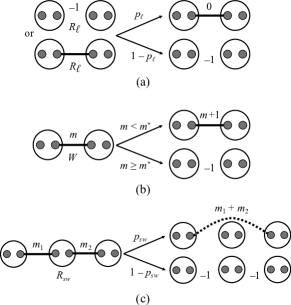
Our implementation of the Q-learning algorithm requires the learning agent to receive a reward in a manner such that maximizing the expected total reward over time corresponds to optimizing either the waiting time or the fidelity. We now provide our definitions of these rewards.
Reward for the waiting time.
When optimizing for the expected waiting time, we want the agent to receive high rewards for actions that bring it to the terminal state, namely, the state in which the two end nodes are connected. Hence, we define the reward as follows:
| (5) |
for every state and action . Note that with this definition, the agent, in order to achieve the highest expected total reward, is incentivized to take the least number of steps to reach the terminal state, and this is why it can be used to minimize the expected waiting time for an end-to-end link.
Reward for the fidelity.
When maximizing the fidelity, we want to give rewards to the Q-learning agent based on minimizing the age of the end-to-end entangled state. Note that when optimizing for the waiting time, the reward in (5) only depends on whether the state is a terminal state. Thus, in that case, the total reward collected is the highest if the number of intermediate states required to reach the terminal states from a fully disconnected initial state is minimized (least number of negative rewards collected). Now, we are not only interested in taking a small number of steps, but also at the end we want to reach a terminal state with a small value of the age of the end-to-end entangled state; we refer to Appendix A for an explanation of the notation . The reward should therefore incentivize the agent to not only reduce the waiting time, but also reduce the age of the end-to-end link. We therefore define the reward as follows:
| (6) |
for every state and action . In other words, higher positive rewards are awarded to the agent if the age of the end-to-end link is low. We also emphasize that by defining the reward in terms of the age of the entangled state, we circumvent the need to keep track of quantum states during our simulations. Let us emphasize a subtlety in the definition of this reward. This reward does not maximize the fidelity alone. In fact, for optimizing the fidelity alone, the optimal policy is clear: just wait for all of the elementary links to become newly active at the same time, and then perform entanglement swapping. This policy maximizes the end-to-end fidelity, but the waiting time is exceedingly large. On the other hand, with the reward function in (6) we can, in a sense, optimize both the fidelity and the waiting time, and we illustrate this explicitly in Sec. IV. We remark that this subtlety in the choice of the reward when considering the fidelity has been pointed out already in the case of elementary links in Ref. [59].
III Improved policies for the waiting time
In this section, we apply the Q-learning reinforcement learning algorithm to find policies that reduce the expected waiting time for end-to-end entanglement in a linear quantum repeater chain. We consider four-node and five-node repeater chains, and we compare the policy obtained via Q-learning to the swap-asap (swap-as-soon-as-possible) policy [49, 50]. We refer to Appendix B for a brief description of the Q-learning algorithm and the details of our implementation of it.
III.1 Evolution of the state and calculation of the waiting time
As described at the beginning of Sec. II, the state of the repeater chain evolves in discrete time steps. Initially, all elementary links in the repeater chain are inactive. In every time step, we have a combination of elementary link requests and requests for entanglement swapping. Specifically, we have the following:
-
1.
Check if there are any elementary link requests. If so, then increase the age of all existing elementary and virtual links by one; see Appendix A for the precise update rule. Otherwise, leave the state unchanged.
-
2.
Perform all requests for elementary links.
-
3.
Perform all entanglement swapping requests.
Since we consider LOCC to be free, any time step in which the action consists only of entanglement swapping requests does not increase the age of existing links and also does not count towards the waiting time. Time steps in which only elementary links are requested or both swaps and elementary links are requested contribute one time step towards the waiting time and also to the age of all links. This is a reasonable assumption for short chains, in which the classical communication time between different nodes of the chain is small compared to the time required to create the elementary links by storing the shared entangled qubits in quantum memories. For longer chains/larger networks, classical communication times become more relevant. Even though we neglect the time taken for entanglement swapping, some reasonable restrictions are put on the allowed actions at any given time step in order to mimic the finite-time requirements of entanglement generation, processing, and storage in memories. Specifically, nodes that request entanglement swapping cannot request elementary links in the same time step, and vice versa. Another restriction is that virtual links cannot cross. For example, consider a seven-link repeater chain. If nodes 1 and 5 are connected, then nodes 2 and 6 cannot be connected; similarly, nodes 3 and 7 cannot be connected, and so on. However, nodes 2, 3, and 4 can form links amongst themselves. We refer to Appendix A for further details regarding the constraints on the states and actions.
III.2 Fixed and dynamic swap-asap policies
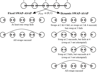
In this work, we consider two versions of the swap-asap policy, one that we refer to as the dynamic swap-asap policy (which has been considered before in Ref. [74]) and the other that we refer to as the fixed swap-asap policy (which has been considered before in Ref. [75]). See Fig. 3 for an illustration of the difference between the two versions.
The dynamic swap-asap policy is defined as follows.
-
•
The action of requesting an elementary link between two neighboring nodes is performed whenever an elementary link is inactive.
-
•
An elementary link is discarded if and only if its age is equal to the maximum cutoff value .
-
•
A virtual link is discarded when its age is equal to .
-
•
Entanglement swaps are performed “as soon as possible”, i.e., as soon as two elementary links sharing a common node are active.
-
•
If more than one entanglement swap can be performed sequentially, then we are free to choose the order of the swaps, in a dynamic way; see Fig. 3 for an example. When LOCC is considered free, all such different orderings correspond to a single time step.
The policy described above is called the “dynamic” swap-asap policy because the entanglement swapping is performed sequentially when multiple entanglement swapping operations can be done at the same time. On the other hand, the fixed swap-asap policy is a strictly local policy in which the entanglement swapping operations are done in parallel rather than sequentially. Doing the entanglement swapping operations in parallel means that they can only succeed together or fail together. For example, in Fig. 3, we see that if one of the entanglement swapping operations fails, then this causes all of the other elementary links to become inactive, even if the swapping succeeds at the other nodes. Instead, in the dynamic swap-asap policy, because the swapping operations are done sequentially, it is possible to communicate the failure of a swapping operation to the adjacent nodes, such the adjacent nodes can avoid doing the entanglement swapping. In fact, a better strategy in the four-segment case is thus to first try to perform the swaps at nodes 2 and 4 and only if they succeed attempt swapping at node 3 (see Fig. 3 (right)). The extra classical communication involved in the dynamic swap-asap policy does not add to the waiting time, because in our model LOCC is considered free. As a result of this freedom in choosing the order of the entanglement swapping, and because LOCC is assumed free, the dynamic swap-asap policy can, in principle, outperform the fixed swap-asap policy.
Despite their differences, from the point of view of actions on elementary links (namely, waiting and requesting on an elementary link), both the fixed and dynamic versions of the swap-asap policy are considered to be local, because in these policies the elementary link actions of waiting and requesting depend only on the state of the nodes performing those actions, and not on the state of the other elementary links or of the network as a whole.
III.3 Homogeneous repeater chains
We now analyze the performance of policies obtained via Q-learning, henceforth referred to as “Q-learning policies”. Specifically, we compare our Q-learning policies to the dynamic swap-asap policy using the improvement factor [75], which is defined as , where is the average waiting time using the Q-learning policy and is the average waiting time using the dynamic swap-asap policy.
Our main results are as follows.
-
1.
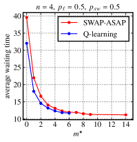
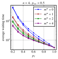
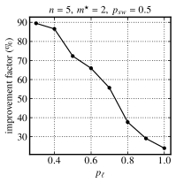
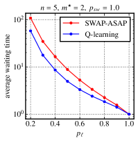
For a fixed elementary link and entanglement swapping success probability, the Q-learning policy’s waiting time curve has a larger gap with the swap-asap curve for smaller values of the maximum memory cutoff . In Fig. 4 (top left), we show this trend for and . As increases, the Q-learning policy approaches the dynamic swap-asap policy, and the improvement factor falls. It is also interesting to note that the waiting time for the dynamic swap-asap policy approaches a fixed value for large . In Fig. 4 (top right), we show that for various values of and , the waiting time falls with increasing values of . We also see that Q-learning policies always yield a lower waiting time than the dynamic swap-asap policy, with the gap reducing with increasing ; see also Fig. 4 (bottom).
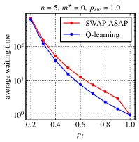
It is also notable that even for , which is when links have to be used as soon as they are created, the Q-learning policy does not coincide with the swap-asap policy. Instead, the Q-learning policy coincides with the policy of waiting for all of the elementary links to become active at the same time, and then doing all of the entanglement swapping operations at once. The waiting time of this policy has the known analytical expression [108] , and this indeed coincides with the Q-learning data shown in Fig. 4 (top right). This result proves that the swap-asap policy is not optimal even in the simple case of . On the other hand, when , the Q-learning and swap-asap policies have the same average waiting time, which is equal to . Although the waiting times coincide, we note that the policies are different, a point that we elaborate upon in Sec. V.1.
-
2.
For deterministic entanglement swapping, in Fig. 5, we observe similar trends, with the Q-learning policies providing a greater advantage for low values of , and the advantage diminishing with increasing . We note that, in this case, both the fixed and dynamic swap-asap policies have the same waiting times. Also, as in the case of non-deterministic entanglement swapping in Fig. 4, it is interesting to see that the swap-asap policy is again not optimal for (see Fig. 5 (right)), while the Q-learning policy has the waiting time given by , corresponding to waiting for all of the elementary links to become active at the same time and then performing all of the entanglement swapping operations at once.
The trends we obtain for the improvement in waiting time in the deterministic swapping case are qualitatively and quantitatively in close agreement with the results in Ref. [75], in which the comparison of their policies was done against the fixed swap-asap policy. This agreement is to be expected, because for deterministic entanglement swapping both the fixed and dynamic swap-asap policies yield the same waiting time. However, in the non-deterministic case, our trends do not agree with Ref. [75], in which the improvement factor increases monotonically with increasing , while in our case the improvement factor decreases. This difference arises because of some of the differences in our assumptions. First, unlike Ref. [75], our MDP formulation allows the memory cutoff to be dynamic, which leads to greater improvement over the policies found in Ref. [75]. Furthermore, since we do not allow requests and swaps at the same nodes to take place in the same time step, our waiting times are slightly different from those found in Ref. [75]. The improvement factors for a five-node repeater chain in Ref. [75] vary between 6-13% for , , and . In our work, for and , the improvement factors against the fixed swap-asap and dynamic swap-asap policies vary between 35-50% and 10-50%, respectively. We have thus shown that by using our more general MDP formulation, a greater improvement in waiting times, even over the dynamic swap-asap policy (which is itself better than the fixed swap-asap policy), can be obtained.
III.4 Inhomogeneous repeater chains


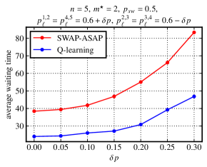
We now consider inhomogeneous quantum repeater chains, in which the elementary link success probabilities are different. We provide the following two sets of results in this setting.
-
1.
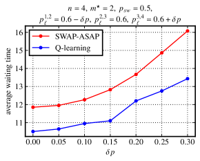
A four-node inhomogeneous repeater chain with all elementary links having different success probabilities , where is the elementary link success probability for pair of adjacent nodes; see Fig. 6. We fix the central elementary link (between nodes 2 and 3) to have , and we vary the other elementary link success probabilities and . We define the inhomogeneity of the chain as . In Fig. 6, we show that our Q-learning policies can improve the average waiting times compared to the dynamic swap-asap policy. The dependence of the improvement on does not have a monotonic trend, but overall, more advantage can be gained in the more asymmetric case. The improvement factor varies between 2% and 8% in this specific case.
-
2.
Next, we consider a five-node inhomogeneous repeater chain that includes central links (elementary links emanating from the central node of the chain) that have low success probability, and outer elementary links that have high success probability; see Fig. 7. In particular, the first and fourth elementary links have high success probability compared to the interior and central links: and , where as before quantifies the inhomogeneity of the chain. This configuration mimics a quantum network built out of short (high ) local elementary links amongst client nodes and long (low ) elementary links to a central hub that connects to several clusters of nodes or small local networks. We consider non-deterministic entanglement swapping, with . In Fig. 7, we show that even in this inhomogeneous setting our Q-learning policies improve upon the dynamic swap-asap policy. The average waiting time improvement factor varies between 26% and 38% for this case. Therefore, as in the case of homogeneous repeater chains, a greater advantage can be gained for longer chains by using our Q-learning policies.
IV Improved policies for the fidelity
We now look at another figure of merit for the performance of quantum repeater chains, namely, the average age of the end-to-end entangled state, which allows us to determine the fidelity of the end-to-end entangled state with respect to the desired maximally entangled state via (2) and (3). Fidelity-based policy optimization using MDPs was previously presented in Ref. [59] for elementary links (see also Ref. [61, Sec. II]).
We present the results of using the Q-learning algorithm, with the fidelity-based reward as defined in (6). The average age of the end-to-end link is calculated by simulating the learned policy, and the average is performed over multiple runs, each run starting from the state of no active elementary links and letting the network evolve until the end-nodes are connected, just as in the case of average waiting time. We emphasize that the policies obtained in this section, using the reward in (6), will in general be different from the policies obtained in Sec. III based on the waiting time reward in (5), because when using (6) as the reward the agent, while learning, considers not only the total time taken to reach the terminal state (end-to-end entangled state) but also the age/fidelity of the terminal state, once it is reached. This allows us to explore the trade-off between the waiting time and the fidelity, namely, that links that are stored longer will decrease the waiting time for an end-to-end link, at the cost of increasing the average age of the end-to-end entangled state (decreasing its fidelity); conversely, storing the links for less time will decrease the average age (increase the fidelity), but it will increase the waiting time.
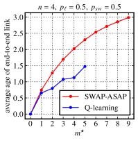
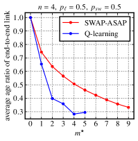
Our results are shown in Fig. 8, Fig. 9, Fig. 10, and Fig. 11. Similar to the case of waiting time, we compare our Q-learning policies to the fixed and dynamic swap-asap policies.
-
1.
In homogeneous repeater chains, we see in Fig. 8 (left) that as the maximum cutoff increases, so too does the average age of the end-to-end link, for both our Q-learning policy and the swap-asap policy; however, the average age remains lower for the Q-learning policy. In particular, as shown in Fig. 8 (right), the ratio between the average age and falls faster for our Q-learning policy than for the swap-asap policy. As we show in Sec. IV.1, the ratio is the key quantity that determines the fidelity of the end-to-end link.
-
2.
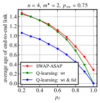
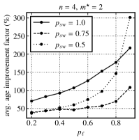
We also find that the average age of the end-to-end entangled state falls with increasing elementary link success probability and increasing swapping probability , as expected. The Q-learning policy reduces the average age of the end-to-end entangled state when compared to both the swap-asap policy and when compared to Q-learning policies based on the waiting time reward in (5); see Fig. 9 (left). Also, in Fig. 9 (left), it is notable that with , our Q-learning policy can obtain a perfect fidelity for the end-to-end-state (average age equal to zero), while with the swap-asap policy this is not possible. We emphasize that this improvement over swap-asap is true for both the waiting time-based Q-learning policy and the fidelity-based Q-learning policy. In particular, even though the waiting time-based Q-learning policy and the swap-asap policy achieve the same average waiting time at , as demonstrated in Fig. 4 (top right), they do not achieve the same average age for the end-to-end link, meaning that the two policies must differ. We elucidate and elaborate on some of these differences in Sec. V.1 below.
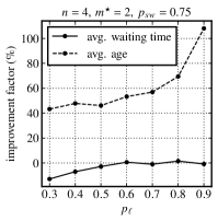
Furthermore, the improvement factor of the average age (compared to the dynamic swap-asap policy), calculated analogously to the waiting time improvement factor, decreases with increasing for deterministic entanglement swapping, whereas it increases with increasing for non-deterministic entanglement swapping; see Fig. 9 (right). It is interesting to see that this trend is different from what we obtain when considering the waiting time reward (see Fig. 4). In particular, as shown in Fig. 10, even though there exists a trade-off between the average waiting time and the average age of the end-to-end link, as described at the beginning of this section, both can be simultaneously improved (in certain parameter regimes) when the Q-learning agent is trained according to the fidelity-based reward in (6).
-
3.
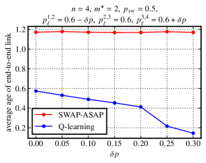
Fig. 11 shows that for inhomogeneous repeater chains, a similar improvement in average age as in homogeneous repeater chains can be obtained from our Q-learning policies. In this case, for some parameter regimes, the average age is enhanced at the expense of larger waiting time (negative improvement), unlike the homogeneous case (Fig. 10) in which both the average age and waiting time could be simultaneously improved.
In Appendix D, we provide an explicit example of a Q-learning policy obtained from our fidelity-based reward in (6), providing the action for every possible state. We compare this policy to the dynamic swap-asap policy and a Q-learning policy obtained from the waiting time reward in (5).
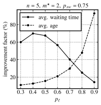
our Q-learning policies become more advantageous for larger chains.
IV.1 Examples
Let us now demonstrate how our Q-learning polices from this section, based on the reward in (6) and formulated abstractly in terms of the age of the end-to-end link, can be used to generate fidelity thresholds for the end-to-end link for given noise models. The primary purpose here is to demonstrate how our abstract theory can be used in practice to analyze the fidelity improvement of our Q-learning policies compared to the swap-asap policy for actual quantum repeater chains.
Noise model.
Our results can be applied to arbitrary Pauli noise models for the decoherence of the memory qubits. For the purposes of this section, we consider the following Pauli noise model:
| (7) |
where are the single-qubit Pauli operators, defined as
| (8) |
and the probabilities are defined as [109, 110]
| (9) | ||||
| (10) | ||||
| (11) | ||||
| (12) |
In this work, because we consider discrete time steps, the quantities represent the discrete analogues of the continuous and times, respectively. Specifically, the quantity represents the coherence time of amplitude damping noise, and represents the coherence time of dephasing noise. We note that, to the best of our knowledge, most prior works consider only dephasing noise [111, 112, 113, 76, 50], while our model is suited to handle arbitrary Pauli noise models, with the specific noise model presented here being only a particular example.
Let us also define the two-qubit Bell states as follows:
| (13) | ||||
| (14) |
Decoherence of an entangled qubit pair.
Now, let us suppose that the initial state of an entangled qubit pair is the perfect maximally-entangled Bell state . We do this for simplicity and illustrative purposes. The following development can be straightforwardly generalized to arbitrary initial entangled qubit pairs whose states have non-unit fidelity; see, e.g., Ref. [61, Appendix C].
After time steps, it is straightforward to show that the decohered entangled state, defined as in (1), is equal to
| (15) |
This implies that the fidelity of the state after time steps is .
Let us now connect the noise model with our MDP model of entanglement distribution, so that we can apply this noise model to the results presented in the previous sections. For a given value of , as used in our MDP model, let us take
| (16) |
In other words, we consider dephasing only for the examples here, in order to make connections to prior works [111, 112, 113, 76, 50] and because dephasing is often the dominant source of noise; see, e.g., Ref. [114]. The fidelity after time steps, given by the function defined in (2), is then equal to
| (17) |
Note that we have chosen the value of in (16) such that, at the cutoff time , the fidelity of the entangled qubit pair is . We emphasize that our results can be applied to other choices of and —in particular, choices that could take amplitude damping into account—in order to obtain a more refined performance analysis.
We can invert the fidelity function in (17), such that for a given fidelity , the corresponding age of the qubits is given by
| (18) |
for all , where we take the ceiling because we want an integer for the age.
We also remark that the decohered entangled state in (15) is a Bell-diagonal state of the form
| (19) |
As such, its entanglement can be characterized entirely by the quantity , namely, the fidelity of the state with respect to . In particular, the state is entangled if and only if this fidelity is greater than or equal to ; see, e.g., [115, Chapter 2]. Therefore, under the assumptions in (16), such that the fidelity is given by (17), we find that the state in (15) is entangled for all time steps .
IV.1.1 Fidelity thresholds
Our Q-learning policies give us lower bounds on the maximum end-to-end fidelity that can be achieved in a repeater chain with a given number of nodes and a given value for the maximum cutoff of the links. For the dephasing model presented above, we use the formula in (17) in order to obtain the fidelity from the age of the end-to-end link; the results are shown in Fig. 12. As already pointed out earlier in this section, we can see that with our Q-learning policies we can achieve perfect fidelity for , while with the swap-asap policy this is not possible.
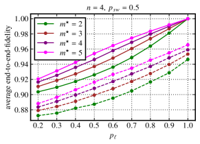
IV.1.2 Performance for low success probabilities
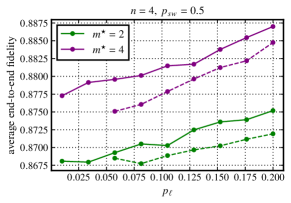
In practice, the elementary link success probability can be quite low—in fact, considerably lower than the values we have considered so far in this work. However, obtaining good policies via reinforcement learning for quantum repeater chains with low values of is generally challenging, requiring many episodes of training. On the other hand, it is of course possible to use the policies obtained through training quantum repeater chains with larger values and apply them to repeater chains with lower values of . Interestingly, as we show in Fig. 13, applying these policies still allows us to obtain an advantage over the swap-asap policy. These results demonstrate the utility of our methods even in the practically relevant setting of low . As an interesting direction for future work, in order to obtain even better fidelity thresholds for low values of , one can train explicitly for these values of by using the policy for a large value of as a “warm start”, in order to potentially make the training easier.
V Discussion of results
In this work, we have considered entanglement distribution in a linear chain of quantum repeaters in the setting of non-deterministic elementary link creation and entanglement swapping. We have done so by modeling the repeater chain using a Markov decision process. Then, using the Q-learning reinforcement learning algorithm, we have obtained policies that improve upon the swap-asap policy, both in terms of the average waiting time and the average age of the end-to-end link, in certain parameter regimes. In addition, by using the Q-learning algorithm, we can explicitly identify the best action for every state, and we provide an example of this in Appendix D. In this section, we provide some details on the high-level insights about our results. In Sec. V.1, we identify some of the key differences between our Q-learning policies and the fixed and dynamic swap-asap policies, which lead to the improvements in waiting time and fidelity shown in Sec. III and Sec. IV. Then, in Sec. V.2, we outline the differences between our work and prior related work on reinforcement learning for entanglement distribution in quantum repeater chains.
V.1 Differences between the swap-asap and Q-learning policies
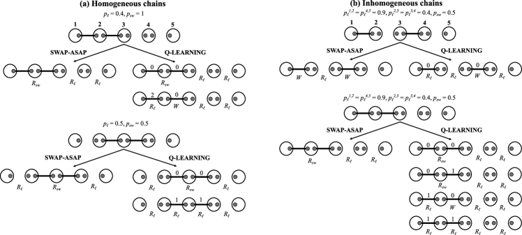
We outline below of the some key differences that we observed between our Q-learning policies and the swap-asap policies. These differences are also illustrated in Fig. 14.
-
1.
For homogeneous repeater chains with deterministic entanglement swapping, it is clear that most of the advantage comes from adopting a “global” policy, in which all of the nodes have knowledge of each other’s states. Specifically, this means that entanglement swapping is not always performed right away, but instead some links will wait until a large number of adjacent nodes are all active. (We quantitatively explore this concept of global knowledge in Sec. VI below.) For an illustration, see Fig. 14(a)(top), where two different age configurations are shown for a five-node chain with maximum cutoff . If both links are fresh, a swap is attempted, but if one of the links is at the maximum cutoff, a swap is not attempted; instead, a new link is requested, because the agent knows that links 3 and 4 are still inactive and will need at least one more time step to become active, by which time the swapped link would have crossed its maximum cutoff time of , according to the rule (see Sec. II). Thus, the second link is saved for one more time step by avoiding an unnecessary swap attempt. More generally, waiting can be advantageous when both the elementary link success probability and the maximum cutoff are low. Indeed, when is low, discarding a link becomes “risky”, because the new elementary link attempt is not likely to succeed. Similarly, when is low, then due to our update rule for the age of a virtual link (see Sec. II), intermediate swapped states will not survive for too long if is low. This also tells us why the advantage of our Q-learning policy is reduced for increasing elementary link success probability and increasing memory cutoff (see Fig. 5).
-
2.
For homogeneous repeater chains with non-deterministic entanglement swapping, as in Fig. 14(a)(bottom), the Q-learning policy often chooses to discard links even before they have reached the maximum cutoff time, in contrast to the dynamic swap-asap policy. For example, in Fig. 14(a)(bottom), segments (2, 3) and (3, 4) are active and (1, 2) and (4, 5) are inactive. The swap-asap policy would attempt a swap at node 3 and request links at (1, 2) and (4, 5). A doubling policy (see Ref. [55] for details) would not perform the swap and just request at (1, 2) and (4, 5). On the other hand, the Q-learning policy chooses several different strategies depending on the absolute and relative ages of the two links and also the values , , , two of which are shown in the figure.
-
3.
For inhomogeneous repeater chains, the key differences in policy occur with respect to the swapping of links with different elementary link success probabilities. This also explains why the improvement factor increases with increasing asymmetry of the chain (see that the gap between the RL and swap-asap curves increases with increasing in Fig. 11). For example, in Fig. 14(b)(top), because the elementary link success probability between the outer nodes 1 and 2 is high, whenever a request for a link between central nodes 2 and 3 is made, the adjacent outer link is also requested even when it is already active. In contrast, in the swap-asap policy (either fixed or dynamic), unless the link is at the cutoff time, it would not be requested. Our Q-learning policy adopts this strategy because it helps keep the outer link fresh, so that whenever the central link is created and a successful swap occurs between it and the adjacent outer link, the age of the virtual link remains low. Otherwise, if the created virtual link has a high age, because the easy-to-produce outer link was old, the precious central link’s lifetime would be effectively shortened. A similar choice of holding off swaps if the effective age of central links would increase due to swapping with an old but easy-to-produce outer link can be seen in Fig. 14(b)(bottom).
V.2 Comparison to prior work
The work presented here is most similar to Refs. [75, 76], in which linear, homogeneous repeater chains are studied. One key difference between those works and ours is that our MDP is different from those in Refs. [75, 76]. In particular, in Ref. [75], the elementary link policy was fixed to the memory-cutoff policy, and only the entanglement swapping policy was optimized. Then, using policy/value iteration, the authors of Ref. [75] obtain policies that improve the average waiting time. On the other hand, although optimization of the elementary link policy is considered in Ref. [76], the authors of that work fix the swapping policy to swap-asap, and they also assume that the entanglement swapping is perfect and deterministic. In this work, we optimize both the policy of the elementary links as well as the policy for the entanglement swapping, and we take as our figure of merit both the average waiting time as well as the fidelity of the end-to-end entangled state. One advantage of our more general MDP is that cutoffs less than the maximum cutoff can be chosen. This then allows implicitly for an optimization of the cutoffs simultaneously with an optimization of the entanglement swapping strategy, in contrast to prior works [62, 76] that perform an optimization of memory cutoffs while keeping the entanglement swapping strategy fixed.
We also emphasize that in this work we use the “addition” update rule for the age of a link after entanglement swapping, while in Ref. [75] the “max” update rule is used. It is known that the addition update rule is the exact update rule for Pauli noise acting on the memory qubits (see Appendix C), while it is unclear whether the max update rule faithfully corresponds to realistic noise models. Our results in Sec. IV therefore provide benchmarks that are meaningful for physically realistic noise models; see specifically Sec. IV.1 above.
Furthermore, in reality, quantum networks will in all likelihood resemble inhomogeneous repeater chains, with elementary links of different lengths, or using different physical platforms/channels, and hence the elementary links would have different success probabilities; see, e.g., Refs. [116, 117]. Thus, in this work we also consider examples of four- and five-node inhomogeneous repeater chains, and we find improved policies for such networks. Finally, the use of the Q-learning algorithm allows us to explicitly extract the learned policy, i.e., a list containing the best action for every possible state (see Appendix D for an example), while for deep reinforcement learning techniques, as used in Ref. [76], extracting the policy is generally difficult.
VI How do improved policies derive their advantage?
In this section, we quantify the various sources of advantage of our Q-learning policies, particularly the advantages that we outlined in the previous section. Broadly, there are three key differences in our improved policies when compared to a fixed-cutoff local swap-asap policy, which are: different cutoffs for the elementary links, global knowledge and coordination between non-adjacent nodes, and decision making with foresight.
VI.1 Non-uniform and state-dependent cutoffs
By analyzing the policies obtained using the Q-learning algorithm, we find that these improved policies have a dynamic and global-state-dependent cutoff for the different elementary links of the network. These cutoffs are, in general, less than the maximum cutoff , which is allowed within our MDP framework; see Sec. II and Appendix A.
In order to see that the cutoffs are not only state dependent but that different links can have different cutoffs, we calculate an average cutoff for every node pair . We do this by averaging the age of a link over instances when it is discarded, i.e., when a link request is performed on that link whenever it is active. Results for four-node and five-node repeater chains are shown in Table 1. We find that, even for homogeneous repeater chains, interior links (closer to the center of the chain) have a higher average cutoff than outer links (closer to the ends of the chain). It appears that the Q-learning agent views the interior links as more “precious” than the outer links. Intuitively, this could be because interior links have the ability to become joined with two links, one on each side, which is not the case for outer links. For inhomogeneous repeater chains, the effect of the difference in the elementary link success probabilities on the choice of the cutoffs can also be seen by looking at the quantities . For a fixed , the choice made by the Q-learning agent is on average smaller for elementary links with higher probability, and vice versa.
The above heuristic can in fact be utilized in a practical setting in the following way. Although our optimized policies choose cutoffs for different links in a dynamic, state-dependent way, it is in general advantageous to choose higher cutoffs for low-probability links and low cutoffs for high-probability links. We can see this just by choosing different but still fixed cutoffs at the elementary link level in the local swap-asap policy. Indeed, waiting times can be reduced and average ages improved, which might seem counter-intuitive to some extent. However, consider for example a four-link chain with elementary link probabilities [0.9, 0.3, 0.3, 0.9]. If we choose a fixed cut-off for all of the links, then we get an average waiting time of and an end-to-end link age of . On the other hand, by reducing the cutoff at links and to , we get a lower waiting time of ( decrease) and an average age of ( decrease). This is a clear example of how the qualitative and quantitative trends that we have identified in our global, optimized policies can be used to modify and improve even local, sub-optimal policies such as the swap-asap policy, without adding very many experimental/engineering challenges.
| link 1 | link 2 | link 3 | |
| 0.6 | 0.6 | 0.6 | |
| 1.3 | 2.0 | 1.4 | |
| 0.3 | 0.6 | 0.9 | |
| 2.0 | 1.0 | 0.15 | |
| link 1 | link 2 | link 3 | link 4 | |
| 0.6 | 0.6 | 0.6 | 0.6 | |
| 0.3 | 0.9 | 1.0 | 0.2 | |
| 0.9 | 0.3 | 0.3 | 0.9 | |
| 0.6 | 2.0 | 2.0 | 0.4 | |
VI.2 Global knowledge and coordination between nodes
Next, we come to global knowledge and the coordination between non-adjacent nodes. It was noted in Sec. III.2 that swap-asap policies use local knowledge of the network to decide on what actions to take. Therefore, only adjacent nodes can coordinate on elementary link requests, waiting, and entanglement swapping requests. On the other hand, in the Q-learning framework, the agent is all-knowing: it can decide on actions based on complete global knowledge of the state of the network. This is one of the main reasons for the improvement over swap-asap, as we demonstrate quantitatively in this section. It is worth mentioning that this source of improvement is already present even within the framework of swap-asap: the fixed version, which is completely local and does not allow for any collaboration, even among adjacent nodes, performs worse than the dynamic version, which allows for some collaboration/flexibility in terms of the decision to do Bell measurements and the order in which swaps are performed.
The extent of global knowledge used in our Q-learning policies can be quantified using correlation functions between actions and states at different links and nodes of the network. Specifically, we use the absolute value of the Pearson correlation coefficient. For two random variables and , it is defined as follows:
| (20) |
where, represents the absolute value, stands for the mean value, and , are the standard deviations of and , respectively. This quantity varies between 0 and 1, with 0 indicating no correlation between the random variables and 1 representing maximum correlation. We calculate this quantity for our Q-learning policies, for the swap-asap policy, and (to provide a baseline) for a random policy, i.e., a policy that consists of a random choice of action for every state. We consider the following cases. We use the notation to denote an action corresponding to the link between nodes and at time , and we use to refer to an action at node at time . Similarly, we use the notation to refer to the state of the link connecting nodes and at time . We refer to Appendix A for more details.
| Correlator | ||||
| N/A | N/A | |||
| N/A | N/A | |||
| N/A | N/A | |||
| N/A | ||||
| N/A | ||||
| N/A | ||||
| N/A | ||||
| N/A | ||||
| N/A | ||||
-
1.
If the actions and at some fixed time at two faraway links/nodes are coordinated, then the covariance between them should be strictly greater than zero, i.e.,
(21) From the first two groups of rows of Table 2, it is clear that for the swap-asap policy the correlation between action pairs and falls off very quickly with increasing distance , whereas the correlations for our Q-learning policy survive even between the two ends of the chain. The random policy provides a base or offset level for the correlations. The correlations that exist only because of state and action constraints (see Appendix A) are reflected by this random policy. Also see Appendix E.
-
2.
Similarly, if the action at fixed time at a link or node is correlated with the status of a faraway link, i.e.,
(22) then this would indicate the use of global knowledge of the state by the policy. Here, the status is defined as if , and if . From the final two groups of rows of Table 2, we see that in the case of swap-asap all the correlation is concentrated between the states and actions at the same site, i.e., only local knowledge of the state is being used. On the other hand, for our Q-learning policies, the correlations are well distributed: the actions at a node/link are not only influenced by the state at that link, but by the state of other links. This indicates global knowledge of the state. Again, correlations for a random policy are provided as a base level. For random policies, actions and states have no correlations beyond those arising from the built-in constraints on them in the MDP formulation, as explained in detail in Appendix A.
For both of the correlation functions considered here, we refer the reader to Appendix E for a detailed discussion on their meaning. Also we note here that for equal time correlators, the time at which the correlator is calculated is irrelevant, since, averages of these correlators are calculated over randomly generated states and actions determined for those states by the respective policies.
VI.3 Decision making with foresight
Our Q-learning policies also take future rewards into account, unlike local policies such as swap-asap, since they sometimes decide to take actions that might lead to a worse state in the very next time step, but over a longer time scale, and on average, lead to more frequent and larger network connectivity. This maximization of future rewards on larger time scales, discounting immediate rewards, is quantified in the Bellman equations (see Appendix B) as the discount factor .
The discounting for future rewards can be examined by looking at unequal-time correlators at a given site or between different sites. In particular, if
| (23) |
for large , then this indicates that actions at time are correlated with states at time . Similar conclusions can be drawn if
| (24) |
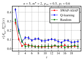
In Fig. 15, we see that for the swap-asap policy, actions at a time are influenced only by the state outcomes at the next time step, and the correlator falls off exponentially with increasing . This indicates that it maximizes only short-term rewards. On the other hand, our Q-learning policy maximizes both short- and long-term rewards through discounting. The unequal-time correlators fall with increasing but are sustained for much longer time scales. The same is true for correlations between different sites. For swap-asap, these correlations are close to zero to begin with (equal-time), and stay so with increasing . In stark contrast, for our Q-learning policies, the non-zero equal-time correlations between states and actions at faraway sites are sustained, even for large . For reference, we provide the correlation coefficient values also for a random policy, i.e., a policy in which an action is chosen randomly for every state. The fact that the initial drop in the correlation function exists for all policies (even the random one) shows that it arises simply due to the MDP rules. The state at always has some correlation with state at time , regardless of the policy, because the MDP rules remain the same. For instance, if one waits at a link that is below its cutoff age, no matter what policy is chosen, the state can never become inactive in the next time step. This correlation dies off quickly for the random and swap-asap policies because the MDP branches off very quickly with time, except for the RL policies, in which some correlation is retained due to foresight. This also explains why this initial high correlation is absent for random and swap-asap policies in Fig. 15 (bottom), because the MDP rules act independently for different links (except for adjacent links involved in a swapping operation). We discuss this and the meaning of foresight in more detail in Appendix E.
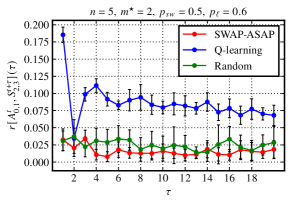
As a side remark, we note that the correlation measure in (23) is similar in spirit to the “empowerment” measure presented in Ref. [118], which considers, instead of the covariance, the mutual information between the random variables and in order to assess a learning agent’s ability to influence its environment.
VII Improved policies for large repeater chains via nesting
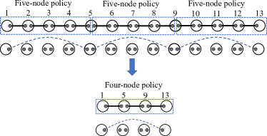
So far, we have considered relatively small repeater chains, up to five nodes, with small values of the maximum cutoff . Remarkably, this has been enough for us to extract general features of policies that outperform the swap-asap policy in certain parameter regimes. Now, we would of course like to obtain policies for larger repeater chains. Doing so, however, becomes quickly intractable, even using reinforcement learning, because the number of states and actions in our MDP grows exponentially with the number of nodes. In this section, we present a method for using policies for small repeater chains in order to construct policies for large repeater chains. This allows us to extend our Q-learning policies to larger repeater chains without having to train over the exponentially large state-action space of such chains. To illustrate the method, we present a specific example with two nesting levels. This makes it clear how to generalize the method to an arbitrary number of nesting levels.
Consider the repeater chain shown in Fig. 16, containing a large number of nodes, and let us split it up into smaller chains, each with nodes. (In Fig. 16, and .) Therefore, the full repeater chain has nodes. Now, our “nesting” policy refers to the use of a given policy for the smaller chains with nodes—this is the “first” nesting level—and then for the “second” nesting level using a policy for nodes. More specifically, the following rules are followed for the two nesting levels.
-
1.
An elementary link request at the second nesting level is considered as a request to create an end-to-end link for the smaller -node chain in the first nesting level. For example, referring to Fig. 16, we regard the chain at the second nesting level to be a four-node chain among the nodes 1, 5, 9, and 13, such that a request for an “elementary link” between nodes 1 and 5 is interpreted as a request for the end-to-end link in the five-node chain, with end nodes 1 and 5, at the first nesting level.
-
2.
All non-terminal states of the first nesting level are considered inactive states for the second nesting level, and once the terminal state in the first/lower level is achieved, its age becomes the age of the elementary link of the second nesting level.
-
3.
Once a request is performed for elementary link generation at the second level, another request is not allowed for that link until it becomes active. The waiting time keeps on increasing in such a case, and any other active links at the second level keep getting older. Lower level links keep evolving as per the policy at that level.
-
4.
Also, like before, an active link at both levels can be discarded anytime as determined by the policy.
-
5.
A new action is performed at the second level only when the state of at least one link at this level changes.
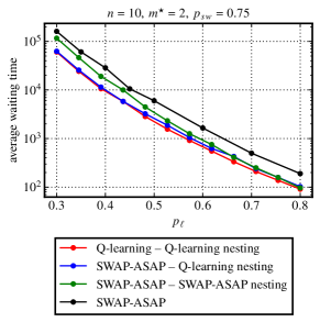
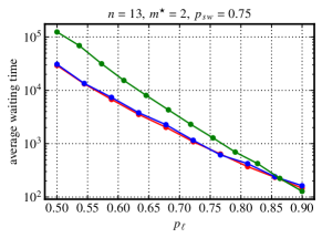
For the budgeting of classical communication time, it is intuitive that any policy for the second nesting level should ideally be local, because nodes at the second nesting level will, in general, be far away from each other, and because global policies require long-distance classical communication, which increases the waiting time. We therefore consider three kinds of nesting of policies for two nesting levels, and we provide examples of the waiting times for these policies for large chains of 10 and 13 nodes in Fig. 17.
-
1.
swap-asap – swap-asap nesting: This is a “local-local” nesting of policies, i.e., the fixed swap-asap policy is used at both levels. This is similar to the “doubling” policy studied in previous literature and is known to be better (in terms of the average waiting time) than a fully local swap-asap policy (without any nesting) for large chains with low elementary link generation success probability and low entanglement swapping success probability [74].
-
2.
swap-asap – Q-learning nesting: This we refer to as a “quasi-local” or “local-global” policy, in which the fixed swap-asap policy is used at the highest (second) nesting level and a Q-learning policy is used at the lowest (first) nesting level. This type of nesting makes sense because, for many repeater chains and network scenarios more generally, it is possible that small sections of the chain (at lower nesting levels) can collaborate amongst themselves and thus use a global policy, without heavily impacting waiting times due to slow classical communication. At the higher (first) level, however, because the corresponding nodes are generally far away, a local policy such as swap-asap should be utilized in order to keep waiting times low. Overall, this type of nesting can reduce waiting times compared to using swap-asap for the full repeater chain. Intuitively, this can also be thought of as increasing the effective link probability of the elementary link of the next nesting level, in turn, reducing the total waiting time. In Fig. 17, we can see that this policy offers a considerable advantage compared to the fully local swap-asap – swap-asap nested policy.
-
3.
Q-learning – Q-learning nesting: This refers to the use of a Q-learning policy at both nesting levels. This is not necessarily a practical policy from the point of view of classical communication time, but it serves as a benchmark to see how advantageous the swap-asap – swap-asap and the swap-asap – Q-learning nested policies can be. In Fig. 17, we see that, in fact, this policy only slightly outperforms the swap-asap – Q-learning nested policies, indicating that the latter is quite efficient in a practical setting.
It is also important to note that all of the nesting policies outperform the simple, non-nested version of dynamic swap-asap; see Fig. 17 (top) for the waiting times of this policy for a 10-node chain. For the 13-node chain (Fig. 17 (bottom)), this simple swap-asap policy performs so poorly that we were unable to obtain any reasonable estimate for the average waiting time, due to the exceedingly long simulation times.
We remark that ideas similar in spirit to our nesting idea can be found in Refs. [63, 119, 73, 120]. Furthermore, from the perspective of Markov decision processes, our nesting idea can be thought of as an example of a multi-agent strategy (as opposed to the single-agent strategy that we have considered throughout this work so far), in which each agent is in charge of a portion of the full chain at the lowest nesting level and acts independently of the other agents. These agents coordinate via another agent at the highest level, which executes a policy that joins the individual portions of the full chain in order to obtain the full end-to-end entanglement.
While we have illustrated our nesting method only for a specific example with two nesting levels, the method can be straightforwardly generalized to an arbitrary number of nesting levels. Also, unlike the example shown here, the repeater chain segments at each nesting level do not have to have the same size. Examining various nesting scenarios for a given repeater chain, in order to determine optimal nesting strategies, is an interesting direction for future work.
VIII Summary and outlook
In this work, we have presented policies for entanglement distribution for linear quantum repeater chains, both homogeneous (with equal elementary link probabilities throughout) and inhomogeneous (in which the elementary link probabilities can be different). We have shown that these policies improve upon the fixed and dynamic versions of the “swap-as-soon-as-possible” (swap-asap) policy, both with respect to the waiting time and the fidelity of the end-to-end entanglement; see Sec. III and Sec. IV. While it might not be surprising that we would obtain improvements, understanding how this improvement comes about is certainly of interest, and it is this question that we have aimed to address in this work. Specifically, we have identified some of the key differences between our policies and the swap-asap policies that lead to these improvements; see Sec. V. We have also quantified three of these key features, namely: state-dependent cutoff times for the elementary and virtual links, collaboration between the nodes, and knowledge of how current actions will affect the state of the repeater chain far in to the future; see Sec. VI. Although we have considered relatively small chains of up to five nodes, and limited values of the maximum cutoff time , this was already enough for us to extract general principles about how the improvement in waiting time and fidelity comes about. We then applied these principles in Sec. VII in order to obtain waiting time improvements for larger repeater chains with 10 and 13 nodes.
We used the Q-learning reinforcement learning algorithm to obtain our improved policies. Q-learning is a model-free reinforcement learning algorithm, unlike model-dependent methods such as value and policy iteration. Drawing an analogy to a game of chess, the agent in Q-learning not only learns the best strategy to win, but does so while learning the rules of the game on the go. This method is thus well suited to situations in which the exact transition probabilities between the different states of a quantum network are either unknown or very difficult to establish, for example in the case of large networks. Furthermore, unlike deep reinforcement learning techniques, the Q-learning algorithm automatically provides us explicitly with the learned policy.
One noteworthy aspect of our results is that the improvement due to our policies is the largest in the most non-ideal cases, that is, when the maximum memory cutoff is small, the elementary link success probabilities are low, and the asymmetries in the repeater chain are the highest. This shows that collaboration between the nodes, one of the central features of our policies, is crucial when dealing with realistic, small-to-medium-scale networks with noisy, imperfect quantum devices.
Our work opens up several interesting avenues for future work. One direction for future work is to add the possibility of doing entanglement distillation, which is a form of quantum error correction, to the MDP formalism presented here. As entanglement distillation is now within the reach of experiments [121, 122, 123], this question is especially pertinent, and much remains to be explored about what policies are optimal in this scenario, building on prior works that have considered specific policies [38, 111, 93, 94, 124, 125, 126, 96]; see also Refs. [71, 72], which numerically investigate several of these scenarios. We therefore expect our insights on the features of improved policies to be a valuable starting point when designing better protocols for quantum repeater chains with multiple memories and entanglement distillation. In particular, it would be interesting to compare a policy that incorporates entanglement distillation to one without entanglement distillation that simply does the memory-cutoff policy with a single memory [72]. It is not obvious that entanglement distillation will always give a better overall fidelity, and understanding in what parameter regimes this is the case will help guide us towards a concept of a noise and loss threshold for quantum communication, similar to the fault-tolerance thresholds for quantum computation that are defined by the point at which the logical error rate of an error-corrected quantum computation is less than the raw, physical error rate.
The analysis in this work considers only the number of nodes in the chain as the input to the problem, and not the physical distances between the nodes. Consequently, the policies we obtain do not explicitly take the actual classical communication time (in physical units of time) into account. While our work still provides an important first step towards understanding what types of policies improve waiting times and fidelities, ultimately, in order for these policies to be useful in practice, we have to take classical communication explicitly into account. One way to do this, albeit indirectly, would be to incorporate the quantifiers considered in Sec. VI into the reward, such that the policies obtained have locality constraints based on the fact that classical communication times between distant nodes can reduce the end-to-end entanglement distribution rate. It would then be interesting to see whether any global-knowledge policy can outperform the local swap-asap policy.
Finally, the ideas in Sec. VII provide an example of using a multi-agent strategy for discovering improved policies in quantum networks. It would be interesting to explore how this nesting strategy, and multi-agent strategies more generally, could be extended to networks with arbitrary topologies, not just linear topologies as we have considered here. Doing so would help guide efforts to develop good policies for arbitrary networks, with the ultimate goal of providing policies for large-scale entanglement distribution, towards a global-scale quantum internet.
Acknowledgements.
The authors thank Paras Regmi and Roy Pace for helpful discussions. This work was supported by the Army Research Office Multidisciplinary University Research Initiative (ARO MURI) through the grant number W911NF2120214. PB and HL also acknowledge the support of the U.S. Air Force Office of Scientific Research as well as the US-Israel Binational Science Foundation. In addition, SK is supported by the German BMBF (Hybrid).References
- Dowling and Milburn [2003] J. P. Dowling and G. J. Milburn, Quantum technology: the second quantum revolution, Philosophical Transactions of the Royal Society of London. Series A: Mathematical, Physical and Engineering Sciences 361, 1655 (2003).
- Van Meter [2014] R. Van Meter, Quantum Networking (John Wiley & Sons, Ltd, 2014).
- Dowling [2020] J. Dowling, Schrödinger’s Web: Race to Build the Quantum Internet (Taylor & Francis, 2020).
- Kimble [2008] H. J. Kimble, The quantum internet, Nature 453 (2008).
- Simon [2017] C. Simon, Towards a global quantum network, Nature Photonics 11, 678 (2017).
- Wehner et al. [2018] S. Wehner, D. Elkouss, and R. Hanson, Quantum internet: A vision for the road ahead, Science 362 (2018).
- Cacciapuoti et al. [2020a] A. S. Cacciapuoti, M. Caleffi, F. Tafuri, F. S. Cataliotti, S. Gherardini, and G. Bianchi, Quantum Internet: Networking Challenges in Distributed Quantum Computing, IEEE Network 34, 137 (2020a), 1810.08421 .
- Illiano et al. [2022] J. Illiano, M. Caleffi, A. Manzalini, and A. S. Cacciapuoti, Quantum Internet protocol stack: A comprehensive survey, Computer Networks 213, 109092 (2022).
- Munro et al. [2022] W. J. Munro, N. L. Piparo, J. Dias, M. Hanks, and K. Nemoto, Designing tomorrow’s quantum internet, AVS Quantum Science 4, 020503 (2022).
- Cirac et al. [1999] J. I. Cirac, A. Ekert, S. F. Huelga, and C. Macchiavello, Distributed quantum computation over noisy channels, Physical Review A 59, 4249 (1999).
- Barz et al. [2012] S. Barz, E. Kashefi, A. Broadbent, J. F. Fitzsimons, A. Zeilinger, and P. Walther, Demonstration of blind quantum computing, Science 335, 303 (2012).
- Ge et al. [2018] W. Ge, K. Jacobs, Z. Eldredge, A. V. Gorshkov, and M. Foss-Feig, Distributed quantum metrology with linear networks and separable inputs, Physical Review Letters 121, 043604 (2018).
- Proctor et al. [2018] T. J. Proctor, P. A. Knott, and J. A. Dunningham, Multiparameter estimation in networked quantum sensors, Physical Review Letters 120, 080501 (2018).
- Komar et al. [2014] P. Komar, E. M. Kessler, M. Bishof, L. Jiang, A. S. Sørensen, J. Ye, and M. D. Lukin, A quantum network of clocks, Nature Physics 10, 582 (2014).
- Gottesman et al. [2012] D. Gottesman, T. Jennewein, and S. Croke, Longer-baseline telescopes using quantum repeaters, Physical Review Letters 109, 070503 (2012).
- Bennett and Brassard [2014] C. H. Bennett and G. Brassard, Quantum cryptography: Public key distribution and coin tossing, Theoretical Computer Science 560, 7 (2014), 2003.06557 .
- Ekert [1991] A. K. Ekert, Quantum cryptography based on Bell’s theorem, Physical Review Letters 67, 661 (1991).
- Xu et al. [2020] F. Xu, X. Ma, Q. Zhang, H.-K. Lo, and J.-W. Pan, Secure quantum key distribution with realistic devices, Reviews of Modern Physics 92, 025002 (2020).
- Pirandola et al. [2020] S. Pirandola, U. L. Andersen, L. Banchi, M. Berta, D. Bunandar, R. Colbeck, D. Englund, T. Gehring, C. Lupo, C. Ottaviani, J. L. Pereira, M. Razavi, J. S. Shaari, M. Tomamichel, V. C. Usenko, G. Vallone, P. Villoresi, and P. Wallden, Advances in quantum cryptography, Advances in Optics and Photonics 12, 1012 (2020), 1906.01645 .
- Heshami et al. [2016] K. Heshami, D. G. England, P. C. Humphreys, P. J. Bustard, V. M. Acosta, J. Nunn, and B. J. Sussman, Quantum memories: emerging applications and recent advances, Journal of Modern Optics 63, 2005 (2016).
- Awschalom et al. [2021] D. Awschalom, K. K. Berggren, H. Bernien, S. Bhave, L. D. Carr, P. Davids, S. E. Economou, D. Englund, A. Faraon, M. Fejer, S. Guha, M. V. Gustafsson, E. Hu, L. Jiang, J. Kim, B. Korzh, P. Kumar, P. G. Kwiat, M. Lončar, M. D. Lukin, D. A. Miller, C. Monroe, S. W. Nam, P. Narang, J. S. Orcutt, M. G. Raymer, A. H. Safavi-Naeini, M. Spiropulu, K. Srinivasan, S. Sun, J. Vučković, E. Waks, R. Walsworth, A. M. Weiner, and Z. Zhang, Development of Quantum Interconnects (QuICs) for Next-Generation Information Technologies, PRX Quantum 2, 017002 (2021).
- Shor [1995] P. W. Shor, Scheme for reducing decoherence in quantum computer memory, Physical Review A 52, R2493 (1995).
- Shor [1996] P. W. Shor, Fault-tolerant quantum computation, in Proceedings of 37th Conference on Foundations of Computer Science (1996) pp. 56–65, quant-ph/9605011 .
- Gottesman [2009] D. Gottesman, An Introduction to Quantum Error Correction and Fault-Tolerant Quantum Computation, arXiv:0904.2557 (2009).
- Roffe [2019] J. Roffe, Quantum error correction: an introductory guide, Contemporary Physics 60, 226 (2019), 1907.11157 .
- Bennett et al. [1996a] C. H. Bennett, H. J. Bernstein, S. Popescu, and B. Schumacher, Concentrating partial entanglement by local operations, Physical Review A 53, 2046 (1996a).
- Bennett et al. [1996b] C. H. Bennett, G. Brassard, S. Popescu, B. Schumacher, J. A. Smolin, and W. K. Wootters, Purification of Noisy Entanglement and Faithful Teleportation via Noisy Channels, Physical Review Letters 76, 722 (1996b).
- Bennett et al. [1996c] C. H. Bennett, D. P. DiVincenzo, J. A. Smolin, and W. K. Wootters, Mixed-state entanglement and quantum error correction, Physical Review A 54, 3824 (1996c).
- Preskill [2018] J. Preskill, Quantum Computing in the NISQ era and beyond, Quantum 2, 79 (2018).
- Bharti et al. [2022] K. Bharti, A. Cervera-Lierta, T. H. Kyaw, T. Haug, S. Alperin-Lea, A. Anand, M. Degroote, H. Heimonen, J. S. Kottmann, T. Menke, W.-K. Mok, S. Sim, L.-C. Kwek, and A. Aspuru-Guzik, Noisy intermediate-scale quantum algorithms, Reviews of Modern Physics 94, 015004 (2022).
- Cerezo et al. [2021] M. Cerezo, A. Arrasmith, R. Babbush, S. C. Benjamin, S. Endo, K. Fujii, J. R. McClean, K. Mitarai, X. Yuan, L. Cincio, and P. J. Coles, Variational quantum algorithms, Nature Reviews Physics 3, 625 (2021).
- Sharma et al. [2020] K. Sharma, S. Khatri, M. Cerezo, and P. J. Coles, Noise resilience of variational quantum compiling, New Journal of Physics 22, 043006 (2020).
- Gentini et al. [2020] L. Gentini, A. Cuccoli, S. Pirandola, P. Verrucchi, and L. Banchi, Noise-resilient variational hybrid quantum-classical optimization, Physical Review A 102, 052414 (2020).
- Fontana et al. [2021] E. Fontana, N. Fitzpatrick, D. M. n. Ramo, R. Duncan, and I. Rungger, Evaluating the noise resilience of variational quantum algorithms, Physical Review A 104, 022403 (2021).
- Cai et al. [2022] Z. Cai, R. Babbush, S. C. Benjamin, S. Endo, W. J. Huggins, Y. Li, J. R. McClean, and T. E. O’Brien, Quantum Error Mitigation, arXiv:2210.00921 (2022).
- Bravyi et al. [2020] S. Bravyi, D. Gosset, R. König, and M. Tomamichel, Quantum advantage with noisy shallow circuits, Nature Physics 16, 1040 (2020).
- Briegel et al. [1998] H.-J. Briegel, W. Dür, J. I. Cirac, and P. Zoller, Quantum Repeaters: The Role of Imperfect Local Operations in Quantum Communication, Physical Review Letters 81, 5932 (1998).
- Dür et al. [1999] W. Dür, H.-J. Briegel, J. I. Cirac, and P. Zoller, Quantum repeaters based on entanglement purification, Physical Review A 59, 169 (1999).
- Muralidharan et al. [2016] S. Muralidharan, L. Li, J. Kim, N. Lütkenhaus, M. D. Lukin, and L. Jiang, Optimal architectures for long distance quantum communication, Scientific Reports 6, 1 (2016).
- Munro et al. [2015] W. J. Munro, K. Azuma, K. Tamaki, and K. Nemoto, Inside Quantum Repeaters, IEEE Journal of Selected Topics in Quantum Electronics 21, 78 (2015).
- Bennett et al. [1993] C. H. Bennett, G. Brassard, C. Crépeau, R. Jozsa, A. Peres, and W. K. Wootters, Teleporting an unknown quantum state via dual classical and Einstein-Podolsky-Rosen channels, Physical Review Letters 70, 1895 (1993).
- Żukowski et al. [1993] M. Żukowski, A. Zeilinger, M. A. Horne, and A. K. Ekert, ‘Event-ready-detectors’ Bell experiment via entanglement swapping, Physical Review Letters 71, 4287 (1993).
- Olmschenk et al. [2009] S. Olmschenk, D. Matsukevich, P. Maunz, D. Hayes, L.-M. Duan, and C. Monroe, Quantum teleportation between distant matter qubits, Science 323, 486 (2009).
- Nölleke et al. [2013] C. Nölleke, A. Neuzner, A. Reiserer, C. Hahn, G. Rempe, and S. Ritter, Efficient teleportation between remote single-atom quantum memories, Physical review letters 110, 140403 (2013).
- Langenfeld et al. [2021] S. Langenfeld, S. Welte, L. Hartung, S. Daiss, P. Thomas, O. Morin, E. Distante, and G. Rempe, Quantum teleportation between remote qubit memories with only a single photon as a resource, Physical Review Letters 126, 130502 (2021).
- Humphreys et al. [2018] P. C. Humphreys, N. Kalb, J. P. Morits, R. N. Schouten, R. F. Vermeulen, D. J. Twitchen, M. Markham, and R. Hanson, Deterministic delivery of remote entanglement on a quantum network, Nature 558, 268 (2018).
- Pfaff et al. [2014] W. Pfaff, B. J. Hensen, H. Bernien, S. B. van Dam, M. S. Blok, T. H. Taminiau, M. J. Tiggelman, R. N. Schouten, M. Markham, D. J. Twitchen, et al., Unconditional quantum teleportation between distant solid-state quantum bits, Science 345, 532 (2014).
- Hermans et al. [2022] S. Hermans, M. Pompili, H. Beukers, S. Baier, J. Borregaard, and R. Hanson, Qubit teleportation between non-neighbouring nodes in a quantum network, Nature 605, 663 (2022).
- Coopmans [2021] T. Coopmans, Tools for the design of quantum repeater networks, Ph.D. thesis, Delft University of Technology (2021), https://repository.tudelft.nl/islandora/object/uuid:90d06f1d-4f23-48cc-8f96-51500258020f?collection=research.
- Kamin et al. [2022] L. Kamin, E. Shchukin, F. Schmidt, and P. van Loock, Exact rate analysis for quantum repeaters with imperfect memories and entanglement swapping as soon as possible, arXiv:2203.10318 (2022).
- Puterman [2014] M. L. Puterman, Markov Decision Processes: Discrete Stochastic Dynamic Programming, Wiley Series in Probability and Statistics (Wiley, 2014).
- Sutton and Barto [2018] R. S. Sutton and A. G. Barto, Reinforcement Learning: An Introduction, 2nd ed. (MIT Press, 2018).
- Khatri et al. [2019] S. Khatri, C. T. Matyas, A. U. Siddiqui, and J. P. Dowling, Practical figures of merit and thresholds for entanglement distribution in quantum networks, Physical Review Research 1, 023032 (2019).
- Vinay and Kok [2019] S. E. Vinay and P. Kok, Statistical analysis of quantum-entangled-network generation, Physical Review A 99, 042313 (2019).
- Shchukin et al. [2019] E. Shchukin, F. Schmidt, and P. van Loock, Waiting time in quantum repeaters with probabilistic entanglement swapping, Physical Review A 100, 032322 (2019).
- Vardoyan et al. [2020] G. Vardoyan, S. Guha, P. Nain, and D. Towsley, On the exact analysis of an idealized quantum switch, Performance Evaluation 144, 102141 (2020).
- Nain et al. [2020] P. Nain, G. Vardoyan, S. Guha, and D. Towsley, On the Analysis of a Multipartite Entanglement Distribution Switch, Proc. ACM Meas. Anal. Comput. Syst. 4 (2020).
- Dai and Towsley [2021] W. Dai and D. Towsley, Entanglement Swapping for Repeater Chains with Finite Memory Sizes, arXiv:2111.10994 (2021).
- Khatri [2021a] S. Khatri, Policies for elementary links in a quantum network, Quantum 5, 537 (2021a).
- Coopmans et al. [2022] T. Coopmans, S. Brand, and D. Elkouss, Improved analytical bounds on delivery times of long-distance entanglement, Physical Review A 105, 012608 (2022).
- Khatri [2022] S. Khatri, On the design and analysis of near-term quantum network protocols using Markov decision processes, arXiv:2207.03403 (2022).
- Li et al. [2020] B. Li, T. Coopmans, and D. Elkouss, Efficient optimization of cut-offs in quantum repeater chains, in 2020 IEEE International Conference on Quantum Computing and Engineering (QCE) (IEEE, 2020) pp. 158–168.
- Jiang et al. [2007] L. Jiang, J. M. Taylor, N. Khaneja, and M. D. Lukin, Optimal approach to quantum communication using dynamic programming, Proceedings of the National Academy of Sciences 104, 17291 (2007).
- da Silva et al. [2021] F. F. da Silva, A. Torres-Knoop, T. Coopmans, D. Maier, and S. Wehner, Optimizing entanglement generation and distribution using genetic algorithms, Quantum Science and Technology 6, 035007 (2021).
- Mailloux et al. [2015] L. O. Mailloux, J. D. Morris, M. R. Grimaila, D. D. Hodson, D. R. Jacques, J. M. Colombi, C. V. Mclaughlin, and J. A. Holes, A Modeling Framework for Studying Quantum Key Distribution System Implementation Nonidealities, IEEE Access 3, 110 (2015).
- Dahlberg and Wehner [2018] A. Dahlberg and S. Wehner, SimulaQron—a simulator for developing quantum internet software, Quantum Science and Technology 4, 015001 (2018).
- Bartlett [2018] B. Bartlett, A distributed simulation framework for quantum networks and channels, arXiv:1808.07047 (2018).
- Matsuo [2019] T. Matsuo, Simulation of a Dynamic, RuleSet-based Quantum Network, arXiv:1908.10758 (2019).
- DiAdamo et al. [2020] S. DiAdamo, J. Nötzel, B. Zanger, and M. M. Beşe, QuNetSim: A Software Framework for Quantum Networks, arXiv:2003.06397 (2020).
- Wu et al. [2020] X. Wu, A. Kolar, J. Chung, D. Jin, T. Zhong, R. Kettimuthu, and M. Suchara, SeQUeNCe: A Customizable Discrete-Event Simulator of Quantum Networks, arXiv:2009.12000 (2020).
- Coopmans et al. [2021] T. Coopmans, R. Knegjens, A. Dahlberg, D. Maier, L. Nijsten, J. Oliveira, M. Papendrecht, J. Rabbie, F. Rozpędek, M. Skrzypczyk, L. Wubben, W. de Jong, D. Podareanu, A. T. Knoop, D. Elkouss, and S. Wehner, NetSquid, a NETwork Simulator for QUantum Information using Discrete events, Communications Physics 4, 164 (2021).
- Wallnöfer et al. [2022a] J. Wallnöfer, F. Hahn, F. Wiesner, N. Walk, and J. Eisert, ReQuSim: Faithfully simulating near-term quantum repeaters, arXiv:2212.03896 (2022a).
- Wallnöfer et al. [2020] J. Wallnöfer, A. A. Melnikov, W. Dür, and H. J. Briegel, Machine Learning for Long-Distance Quantum Communication, PRX Quantum 1, 010301 (2020).
- Shchukin and van Loock [2022] E. Shchukin and P. van Loock, Optimal entanglement swapping in quantum repeaters, Physical Review Letters 128, 150502 (2022).
- Iñesta et al. [2022] Á. G. Iñesta, G. Vardoyan, L. Scavuzzo, and S. Wehner, Optimal entanglement distribution policies in homogeneous repeater chains with cutoffs, arXiv:2207.06533 (2022).
- Reiß and van Loock [2022] S. D. Reiß and P. van Loock, Deep reinforcement learning for key distribution based on quantum repeaters, arXiv:2207.09930 (2022).
- Holevo [2012] A. S. Holevo, Quantum Systems, Channels, Information: A Mathematical Introduction (Walter de Gruyter GmbH, 2012).
- Nielsen and Chuang [2000] M. A. Nielsen and I. L. Chuang, Quantum Computation and Quantum Information (Cambridge University Press, 2000).
- Khatri and Wilde [2020] S. Khatri and M. M. Wilde, Principles of Quantum Communication Theory: A Modern Approach, arXiv:2011.04672 (2020).
- Bäuml et al. [2015] S. Bäuml, M. Christandl, K. Horodecki, and A. Winter, Limitations on quantum key repeaters, Nature Communications 6, 6908 (2015).
- Pirandola [2016] S. Pirandola, Capacities of repeater-assisted quantum communications, arXiv:1601.00966 (2016).
- Azuma et al. [2016] K. Azuma, A. Mizutani, and H.-K. Lo, Fundamental rate-loss trade-off for the quantum internet, Nature Communications 7, 13523 (2016).
- Laurenza and Pirandola [2017] R. Laurenza and S. Pirandola, General bounds for sender-receiver capacities in multipoint quantum communications, Physical Review A 96, 032318 (2017).
- Christandl and Müller-Hermes [2017] M. Christandl and A. Müller-Hermes, Relative Entropy Bounds on Quantum, Private and Repeater Capacities, Communications in Mathematical Physics 353, 821 (2017).
- Azuma and Kato [2017] K. Azuma and G. Kato, Aggregating quantum repeaters for the quantum internet, Physical Review A 96, 032332 (2017).
- Bäuml and Azuma [2017] S. Bäuml and K. Azuma, Fundamental limitation on quantum broadcast networks, Quantum Science and Technology 2, 024004 (2017).
- Rigovacca et al. [2018] L. Rigovacca, G. Kato, S. Bäuml, M. S. Kim, W. J. Munro, and K. Azuma, Versatile relative entropy bounds for quantum networks, New Journal of Physics 20, 013033 (2018).
- Pirandola [2019a] S. Pirandola, End-to-end capacities of a quantum communication network, Communications Physics 2, 51 (2019a).
- Pirandola [2019b] S. Pirandola, Bounds for multi-end communication over quantum networks, Quantum Science and Technology 4, 045006 (2019b).
- Das et al. [2021] S. Das, S. Bäuml, M. Winczewski, and K. Horodecki, Universal Limitations on Quantum Key Distribution over a Network, Physical Review X 11, 041016 (2021).
- Bäuml et al. [2020] S. Bäuml, K. Azuma, G. Kato, and D. Elkouss, Linear programs for entanglement and key distribution in the quantum internet, Communications Physics 3, 55 (2020).
- Harney and Pirandola [2022] C. Harney and S. Pirandola, Analytical methods for high-rate global quantum networks, PRX Quantum 3, 010349 (2022).
- Van Meter et al. [2009] R. Van Meter, T. D. Ladd, W. J. Munro, and K. Nemoto, System Design for a Long-Line Quantum Repeater, IEEE/ACM Transactions on Networking 17, 1002 (2009).
- Aparicio et al. [2011] L. Aparicio, R. Van Meter, and H. Esaki, Protocol Design for Quantum Repeater Networks, in Proceedings of the 7th Asian Internet Engineering Conference, AINTEC ’11 (Association for Computing Machinery, New York, NY, USA, 2011) pp. 73–80.
- Jones et al. [2016] C. Jones, D. Kim, M. T. Rakher, P. G. Kwiat, and T. D. Ladd, Design and analysis of communication protocols for quantum repeater networks, New Journal of Physics 18, 083015 (2016).
- Matsuo et al. [2019] T. Matsuo, C. Durand, and R. Van Meter, Quantum link bootstrapping using a ruleset-based communication protocol, Physical Review A 100, 052320 (2019).
- Rozpędek et al. [2018] F. Rozpędek, T. Schiet, L. P. Thinh, D. Elkouss, A. C. Doherty, and S. Wehner, Optimizing practical entanglement distillation, Physical Review A 97, 062333 (2018).
- Krastanov et al. [2019] S. Krastanov, V. V. Albert, and L. Jiang, Optimized Entanglement Purification, Quantum 3, 123 (2019).
- Cacciapuoti et al. [2020b] A. S. Cacciapuoti, M. Caleffi, R. Van Meter, and L. Hanzo, When Entanglement Meets Classical Communications: Quantum Teleportation for the Quantum Internet, IEEE Transactions on Communications 68, 3808 (2020b), 1907.06197 .
- Dai et al. [2020] W. Dai, T. Peng, and M. Z. Win, Optimal Remote Entanglement Distribution, IEEE Journal on Selected Areas in Communications 38, 540 (2020).
- Chakraborty et al. [2020] K. Chakraborty, D. Elkouss, B. Rijsman, and S. Wehner, Entanglement Distribution in a Quantum Network, a Multi-Commodity Flow-Based Approach, arXiv:2005.14304 (2020).
- Goodenough et al. [2021] K. Goodenough, D. Elkouss, and S. Wehner, Optimizing repeater schemes for the quantum internet, Physical Review A 103, 032610 (2021).
- Bugalho et al. [2021] L. Bugalho, B. C. Coutinho, F. A. Monteiro, and Y. Omar, Distributing Multipartite Entanglement over Noisy Quantum Networks, arXiv:2103.14759 (2021).
- Miguel-Ramiro et al. [2021] J. Miguel-Ramiro, A. Pirker, and W. Dür, Optimized Quantum Networks, arXiv:2107.10275 (2021).
- Azuma et al. [2021] K. Azuma, S. Bäuml, T. Coopmans, D. Elkouss, and B. Li, Tools for quantum network design, AVS Quantum Science 3, 014101 (2021).
- Bowen and Bose [2001] G. Bowen and S. Bose, Teleportation as a Depolarizing Quantum Channel, Relative Entropy, and Classical Capacity, Physical Review Letters 87, 267901 (2001).
- Schmidt and van Loock [2020] F. Schmidt and P. van Loock, Memory-assisted long-distance phase-matching quantum key distribution, Physical Review A 102, 042614 (2020).
- Das et al. [2018] S. Das, S. Khatri, and J. P. Dowling, Robust quantum network architectures and topologies for entanglement distribution, Physical Review A 97, 012335 (2018).
- Sarvepalli et al. [2009] P. K. Sarvepalli, A. Klappenecker, and M. Rötteler, Asymmetric quantum codes: constructions, bounds and performance, Proceedings of the Royal Society A: Mathematical, Physical and Engineering Sciences 465, 1645 (2009), https://www.jstor.org/stable/30243785 .
- Ghosh et al. [2012] J. Ghosh, A. G. Fowler, and M. R. Geller, Surface code with decoherence: An analysis of three superconducting architectures, Physical Review A 86, 062318 (2012), 1210.5799 .
- Razavi et al. [2009] M. Razavi, M. Piani, and N. Lütkenhaus, Quantum repeaters with imperfect memories: Cost and scalability, Physical Review A 80, 032301 (2009).
- Rozpędek et al. [2018] F. Rozpędek, K. Goodenough, J. Ribeiro, N. Kalb, V. C. Vivoli, A. Reiserer, R. Hanson, S. Wehner, and D. Elkouss, Parameter regimes for a single sequential quantum repeater, Quantum Science and Technology 3, 034002 (2018), 1705.00043 .
- Rozpędek et al. [2019] F. Rozpędek, R. Yehia, K. Goodenough, M. Ruf, P. C. Humphreys, R. Hanson, S. Wehner, and D. Elkouss, Near-term quantum-repeater experiments with nitrogen-vacancy centers: Overcoming the limitations of direct transmission, Physical Review A 99, 052330 (2019).
- Ourari et al. [2023] S. Ourari, l. Dusanowski, S. P. Horvath, M. T. Uysal, C. M. Phenicie, P. Stevenson, M. Raha, S. Chen, R. J. Cava, N. P. de Leon, and J. D. Thompson, Indistinguishable telecom band photons from a single Er ion in the solid state, Nature 620, 977 (2023).
- Khatri [2021b] S. Khatri, Towards a General Framework for Practical Quantum Network Protocols, Ph.D. thesis, Louisiana State University (2021b), https://digitalcommons.lsu.edu/gradschool_dissertations/5456/.
- Khatri et al. [2021] S. Khatri, A. J. Brady, R. A. Desporte, M. P. Bart, and J. P. Dowling, Spooky action at a global distance: analysis of space-based entanglement distribution for the quantum internet, npj Quantum Information 7, 4 (2021).
- Wallnöfer et al. [2022b] J. Wallnöfer, F. Hahn, M. Gündoǧan, J. S. Sidhu, F. Wiesner, N. Walk, J. Eisert, and J. Wolters, Simulating quantum repeater strategies for multiple satellites, Communications Physics 5, 169 (2022b).
- Klyubin et al. [2005] A. Klyubin, D. Polani, and C. Nehaniv, Empowerment: a universal agent-centric measure of control, in 2005 IEEE Congress on Evolutionary Computation, Vol. 1 (2005) pp. 128–135.
- Van Meter et al. [2011] R. Van Meter, J. Touch, and D. Horsman, Recursive quantum repeater networks, Progress in Informatics 8, 65 (2011), 1105.1238 .
- Azuma [2023] K. Azuma, Networking quantum networks with minimum cost aggregation, arXiv:2304.08921 (2023).
- Pan et al. [2001] J.-W. Pan, C. Simon, C. Brukner, and A. Zeilinger, Entanglement purification for quantum communication, Nature 410, 1067 (2001).
- Kalb et al. [2017] N. Kalb, A. A. Reiserer, P. C. Humphreys, J. J. W. Bakermans, et al., Entanglement distillation between solid-state quantum network nodes, Science 356, 928 (2017).
- Ruf et al. [2021] M. Ruf, N. H. Wan, H. Choi, D. Englund, and R. Hanson, Quantum networks based on color centers in diamond, Journal of Applied Physics 130, 070901 (2021).
- Bratzik et al. [2013] S. Bratzik, S. Abruzzo, H. Kampermann, and D. Bruß, Quantum repeaters and quantum key distribution: The impact of entanglement distillation on the secret key rate, Physical Review A 87, 062335 (2013).
- Pirker et al. [2018] A. Pirker, J. Wallnöfer, and W. Dür, Modular architectures for quantum networks, New Journal of Physics 20, 053054 (2018).
- Pirker and Dür [2019] A. Pirker and W. Dür, A quantum network stack and protocols for reliable entanglement-based networks, New Journal of Physics 21, 033003 (2019).
- Stewart [2009] W. J. Stewart, Probability, Markov Chains, Queues, and Simulation: The Mathematical Basis of Performance Modeling (Princeton University Press, 2009).
- Watkins [1989] C. J. C. H. Watkins, Learning from Delayed Rewards, Ph.D. thesis, Cambridge University (1989).
- Tsitsiklis [1994] J. N. Tsitsiklis, Asynchronous Stochastic Approximation and Q-Learning, Machine Learning 16, 185 (1994).
- Jaakkola et al. [1994] T. Jaakkola, M. I. Jordan, and S. P. Singh, On the Convergence of Stochastic Iterative Dynamic Programming Algorithms, Neural Computation 6, 1185 (1994).
- Kearns and Singh [1998] M. Kearns and S. Singh, Finite-Sample Convergence Rates for Q-Learning and Indirect Algorithms, in Advances in Neural Information Processing Systems, Vol. 11, edited by M. Kearns, S. Solla, and D. Cohn (MIT Press, 1998).
- Dar and Mansour [2003] E. E. Dar and Y. Mansour, Learning Rates for Q-learning, Journal of Machine Learning Research 5, 1 (2003).
Appendix A Details of the Markov decision process
Here, we provide further details on our Markov decision process (MDP) framework for quantum repeater chains, which is summarized in Fig. 2 of the main text.
A Markov decision process (MDP) [51] (see also Ref. [61, Appendix A]) is a mathematical model of an agent that has the ability to interact with a system by taking different actions on it. The system consists of a set of (classical) states, and similarly the actions form a set . The transition probabilities between states are given by transition matrices , such that the matrix element is equal to the probability of going to the state , when the current state is and the action taken is . We now present these defining elements of an MDP within the context of quantum repeater chains. We also note that our definitions of the states and actions in a quantum repeater chain are similar to, but not exactly the same as, those in Refs. [75, 76]; see Sec. V.2 for details on the differences.
A.1 States
The state space consists of all possible configurations of the repeater chain. In particular, we represent the state of the repeater chain at any given time by an matrix , where is the number of nodes in the chain. The state of the link between two nodes is represented by the entry , which can lie between and , with indicating that the link is active and indicating that the link is inactive.
For example, consider a four-node repeater chain, with an elementary link between node 1 and 2 that is active for one time step and a virtual link between 2 and 4 that is active for two time steps. Such a state is represented as
| (25) |
where the asterisks ‘’ indicate that the corresponding entries could be arbitrary elements in the set . The terminal/absorbing states are states in which the first and the last node are connected by a virtual link. Such states have the form , for .
We remark that not all matrices are possible states of the repeater chain. First, the states are symmetric and nodes cannot link to themselves, so that diagonal elements of the form are not allowed. Furthermore, because we are only dealing with a linear repeater chain in which every node has at most two quantum memories, every node can be connected to not more than two more nodes, one ahead it and one behind it. Therefore, every row and column of can have only two elements that are not equal to . These constraints mean that the number of possible states scales as . For example, for a repeater chain with nodes and maximum cutoff , the number of allowed states is 562.
A.2 Actions
The action space consists of the following.
-
•
Request (): This action is a request to create an elementary link between two adjacent nodes. The success probability of elementary link creation is denoted by . If the elementary link is already active between the two nodes, then this action first discards the link and then attempts to create a new one.
-
•
Wait (): This action keeps a link, either a virtual link or an elementary link, stored in the quantum memories. It increases the age of active links by one; however, if the current age is equal to the maximum cutoff , then the link becomes inactive.
-
•
Request Swapping () : This action can take place at any node when it is linked to two other nodes via elementary or virtual links. We assume that the entanglement swapping is error free but in general non-deterministic, succeeding with probability . If it succeeds, a virtual link is established between the corresponding end nodes. In case of failure, both links become inactive.
Mathematically, similar to the states, we describe the action taken on a state at any given time by an matrix . Now, represents the action taken by the nodes together. This is also a symmetric matrix. An elementary link request () is given by , with . The wait action () is given by for . Entanglement swapping requests () are given by diagonal elements of the matrix, so that means a request for entanglement swapping at the node. For example, consider a four-node repeater chain. The action of requesting an elementary link between node 1 and node 2 along with a swapping request at node 3 is represented as
As with the states, the number of allowed actions is limited. Again, the actions are symmetric, but now the elements can be non-zero. Also, no action is allowed between non-adjacent nodes, so the only non-diagonal non-zero elements are of the form . These constraints bring down the number of possible actions to the order of for a repeater chain with nodes. Further, if a swap action is taken at a node, then the same node is not involved in an elementary link request ; therefore, if , then the row and column can have no other non-zero entry. These constraints reduce the number of allowed actions even more. For example, for a repeater chain with nodes, the number of allowed actions is only 34 (out of the possible actions taking all combinations of elementary link generation and entanglement swap requests).
A.3 Transition rules
Let us now look at the effect of various actions on the states of the repeater chain.
-
•
Effect of request (): If , then with probability we obtain , and with probability we obtain .
-
•
Effect of wait (): If and , then
(26) If the link is already inactive, i.e., if , then . Observe that the action automatically discards any link (elementary or virtual) that has an age equal to the maximum cutoff time .
-
•
Effect of request for entanglement swapping (): If , then check if and , i.e., check if the node has an active link with some nodes and . If so, then with probability , , and with probability , . For both outcomes, the parent links become inactive, i.e., and . Note that if an entanglement swap is requested at a node that is connected to only one other node, then that link becomes inactive. Also, if a swap operation is attempted when , even if the operation succeeds. Therefore, virtual links are always cut-off at the maximum cut-off age.
The request and wait actions effect individual links independently. The swap request, on the other hand, depends on and effects the states of two links.
The transition rules described above form the transition matrices of our MDP. As a result of having absorbing states, we can partition every transition matrix , , into a block matrix as follows:
| (27) |
where the top-left block corresponds to transitions between transient (non-terminal) states, the bottom-left block corresponds to transitions from transient states to terminal states, and the bottom-right block corresponds to transitions between terminal states, which is the identity matrix by our definition of a terminal state.
A.4 Optimization of waiting time and fidelity
A policy is defined by the function , such that is defined as the probability of taking action given that the state of the repeater chain is . In other words, the policy is a collection of conditional probability distributions, one for every state.
For every policy , we define the transition matrix such that, for all ,
| (28) |
Based on the block structure of the transition matrices , as described above, we have that for every policy the transition matrix has the following block structure:
| (29) |
where
| (30) |
for all transient states , and
| (31) |
for all transient states and terminal states .
Optimization of waiting time.
For a given policy , let
| (32) |
Then, it follows from the theory of Markov chains (see, e.g., [127, Theorem 9.6.1]) that the expected time to reach a terminal state (i.e., the expected waiting time for an end-to-end link) is given by
| (33) |
where is the initial probability distribution of (transient) states at time . The minimum expected waiting time is then given by the following optimization problem:
| (34) |
Optimization of fidelity.
For every state of the repeater chain, we define
| (35) |
where we recall the function defined in (2). In other words, gives the fidelity of the end-to-end entangled state, when it is active. We are then interested in the expected value of this quantity with respect to a policy in the steady-state limit:
| (36) | ||||
| (37) |
where in the last line is the initial probability distribution of (transient) states at time . The maximum fidelity is then given by the following optimization problem:
| (38) |
Appendix B The Q-learning algorithm
In this work, we used the Q-learning algorithm [52] to train the learning agent. Q-learning employs the following update rule:
| (39) |
where is the expected return of the state-action pair ( and at time , respectively). The Q-learning algorithm is known to converge to an optimal policy in the limit that all state-action pairs are visited infinitely often [128, 129, 130]. Convergence rates and sampling complexities for Q-learning have been studied in Refs. [131, 132].
The Q-learning algorithm initializes a Q-matrix of dimension |. The initial state is chosen randomly from all possible non-terminal states. Then, the initial action is chosen using an -greedy algorithm, in which the reward is maximized with probability , otherwise a random action is taken. The new Q-value for the state-action pair is updated in the Q-matrix according to a pre-established reward. The algorithm repeats this cycle until a terminal state is reached; see Fig. 18. This sequence starting from an initial state and reaching the terminal state is defined as an episode. After the algorithm has run over an adequate number of episodes, the column corresponding to the maximum value in the row of the Q-matrix represents the best possible action in the state “”. Hence, the Q-matrix explicitly determines the improved policy.

Role of training hyperparameters in learning.
Four training hyperparameters, namely , and the number of training episodes, need to be tuned in order to find improved policies.
-
1.
The role of is to determine the learning rate. A very low makes the training too slow; a very large makes us “overshoot” the optimal policy. A value of was found to be ideal for training in this work.
-
2.
The discount factor determines the discounting for future rewards. This parameter also needs to be tuned in order to find a good balance between prioritizing immediate (next state) rewards versus long-term rewards. We found to be ideal.
-
3.
The hyperparameter , as mentioned above, controls the trade-off between the exploration of the agent (choosing random actions) and its exploitation (using learned actions). We found to be the most relevant hyperparameter, and the one that requires the most fine tuning for finding improved policies. We found to be optimal.
-
4.
The figures of merit improve with an increasing number of training episodes (at the expense of a higher training time) until they saturate and more training does not help. Furthermore, the larger the state-action space (i.e., the higher the number of nodes and/or the maximum cutoff ), and the smaller the probability of creating elementary and virtual links (small , ), the larger the number of training episodes required for getting an improved policy. The number of training episodes needed for saturating the figures of merit varied between a few hundred thousand to approximately one million.
Here we also note that training need not be done for the entire range of repeater chain parameters that need to be simulated. Our Q-learning policies are different for different values of , , etc., but they are not very sensitive to small changes in these parameters. For example, to simulate the repeater chain for , we trained and determined the policy only for . Training separately for , and then using those policies, gave no improvement in the waiting time or fidelity compared to using the policy. We can view this as an example of “transferable reinforcement learning”, and we could also use policies for one value of in order to “warm start” the training for another value of , in order to improve training times. This is especially relevant to finding policies for chains with very small values of and , for which training from scratch is extremely resource intensive.
Verification of the Q-learning algorithm for a single elementary link.
At the elementary link level, if one assumes a finite memory cutoff, the improved policy is to request () until the link is created and then wait for time steps before requesting again. For the single link, analytical expressions for figures of merit such as expected state of the link or average wait times can be obtained (see Corollary 4.3 in Ref. [59]) and show that the aforementioned policy is optimal. As a sanity check, we see in Fig. 19 that the Q-learning algorithm also rediscovers this policy and gives qualitative and quantitative agreement with the aforementioned analytical results.
Appendix C Entanglement swapping update rule for Pauli noise
In this section, we prove the formula for the fidelity after entanglement swapping of two entangled states impacted by Pauli noise, with ages and . This formula can be viewed as a special case of the general formula in Ref. [61, Proposition III.1] or as a consequence of the developments in Ref. [107, Appendix D]; however, here we provide a direct proof. To that end, let be an arbitrary Pauli channel, so that
| (40) |
where are probabilities and are the single-qubit Pauli operators. Consider noisy bipartite states with ages and , as defined in (1):
| (41) | ||||
| (42) |
with the qubits and being involved in the entanglement swapping operation. Using the property that for every linear operator , we can write these states as
| (43) | ||||
| (44) |
such that for the first state the noise acts entirely on qubit and for the second state the noise acts entirely on qubit . Now, the entanglement swapping operation can be represented as the following quantum channel [61, Sec. III.B.1]:
| (45) |
where . Then, because the Pauli corrections being applied to the qubit as part of the entanglement swapping protocol are themselves Pauli channels, it holds that these channels commute with the noise channel , which means that
| (46) | |||
| (47) | |||
| (48) | |||
| (49) | |||
| (50) | |||
| (51) |
Appendix D Comparing the swap-asap policy with Q-learning policies
In Sec. V, we compared our Q-learning policies with the fixed and dynamic swap-asap policies. Our Q-learning policies are based on two different rewards. The first reward is based on optimizing the average waiting time alone (see (5)), and the second reward is based on optimizing both the average waiting time and the fidelity of the end-to-end entangled state (see (6)). In Table LABEL:Q_table, we compare these improved policies with each other and also with the dynamic swap-asap policy. Since the dynamic swap-asap policy allows freedom in the order of swaps (see Sec. III.2) when an action consisting of two swap requests is taken, these swaps are performed sequentially, i.e., if the first swap fails the second one is not performed. On the other hand, for the Q-learning policies, such freedom is not allowed. All swaps that are requested by the policy are performed in one go. This is in keeping with our assumptions that Q-learning is free to find the optimal order of actions, which includes the order of swaps. In the case as shown in the table below, the Q-learning policies do in fact choose to perform the swaps in one go.
| State | Q-learning action (waiting time) | Q-learning action (fidelity & waiting time) | swap-asap action |
| (, , ) | (, , ) | (, , ) | (, , ) |
| (, , ) | (, , ) | (, , ) | (, , ) |
| (, , ) | (, , ) | (, , ) | (, , ) |
| (, , ) | (, , ) | (, , ) | (, , ) |
| (, ) | (, ) | (, ) | (, ) |
| (, ) | (, ) | (, ) | (, ) |
| (, ) | (, , ) | (, , ) | (, , ) |
| (, 0, ) | (, , ) | (, , ) | (, , ) |
| (, 0, 0) | (, ) | (, ) | (, ) |
| (, 0, 1) | (, ) | (, , ) | (, ) |
| (, 0, 2) | (, , ) | (, , ) | (, ) |
| (, 1, ) | (, , ) | (, , ) | (, , ) |
| (, 1, 0) | (, ) | (, , ) | (, ) |
| (, 1, 1) | (, , ) | (, , ) | (, ) |
| (, 1, 2) | (, , ) | (, , ) | (, ) |
| (, 2, ) | (, , ) | (, , ) | (, , ) |
| (, 2, 0) | (, , ) | (, , ) | (, ) |
| (, 2, 1) | (, , ) | (, , ) | (, ) |
| (, 2, 2) | (, , ) | (, , ) | (, ) |
| 0 - (, , ) | N/A | N/A | N/A |
| 0 - (, 0, ) | N/A | N/A | N/A |
| 0 - (, 1, ) | N/A | N/A | N/A |
| 0 - (, 2, ) | N/A | N/A | N/A |
| 1 - (, , ) | N/A | N/A | N/A |
| 1 - (, 0, ) | N/A | N/A | N/A |
| 1 - (, 1, ) | N/A | N/A | N/A |
| 1 - (, 2, ) | N/A | N/A | N/A |
| 2 - (, , ) | N/A | N/A | N/A |
| 2 - (, 0, ) | N/A | N/A | N/A |
| 2 - (, 1, ) | N/A | N/A | N/A |
| 2 - (, 2, ) | N/A | N/A | N/A |
| (0, ) | (, ) | (, ) | (, |
| (0, 0) | |||
| (0, 1) | |||
| (0, 2) | |||
| (1, ) | (, ) | (, ) | (, ) |
| (1, 0) | |||
| (1, 1) | |||
| (1, 2) | (, , ) | (, , ) | |
| (2, ) | (, , ) | (, , ) | (, , ) |
| (2, 0) | |||
| (2, 1) | (, ) | (, ) | (, ) |
| (2, 2) | (, , ) | (, , ) | |
| (0, , ) | (, , ) | (, , ) | (, , ) |
| (0, , 0) | (, , ) | (, , ) | (, , ) |
| (0, , 1) | (, , ) | (, , ) | (, , ) |
| (0, , 2) | (, , ) | (, , ) | (, , ) |
| (0, 0, ) | (, ) | (, ) | (, ) |
| (0, 0, 0) | (, ) | (, ) | (, ) |
| (0, 0, 1) | (, ) | (, ) | (, ) |
| (0, 0, 2) | (, ) | (, ) | (, ) |
| (0, 1, ) | (, ) | (, ) | (, ) |
| (0, 1, 0) | (, ) | (, ) | (, ) |
| (0, 1, 1) | (, ) | (, ) | (, ) |
| (0, 1, 2 ) | (, ) | (, ) | (, ) |
| (0, 2, ) | (, , ) | (, , ) | (, ) |
| (0, 2, 0) | (, ) | (, ) | (, ) |
| (0, 2, 1) | (, , ) | (, , ) | (, ) |
| (0, 2, 2) | (, , ) | (, , ) | (, ) |
| (1, , ) | (, , ) | (, , ) | (, ) |
| (1, , 0) | (, , ) | (, , ) | (, , ) |
| (1, , 1) | (, , ) | (, , ) | (, , ) |
| (1, , 2) | (, , ) | (, , ) | (, , ) |
| (1, 0, ) | (, ) | (, , ) | (, ) |
| (1, 0, 0) | (, ) | (, ) | (, ) |
| (1, 0, 1) | (, ) | (, ) | (, ) |
| (1, 0, 2) | (, ) | (, ) | (, ) |
| (1, 1, ) | (, ) | (, , ) | (, ) |
| (1, 1, 0) | (, ) | (, ) | (, ) |
| (1, 1, 1) | (, , ) | (, , ) | (, ) |
| (1, 1, 2) | (, , ) | (, , ) | (, ) |
| (1, 2, ) | (, , ) | (, , ) | (, ) |
| (1, 2, 0) | (, , ) | (, , ) | (, ) |
| (1, 2, 1) | (, , ) | (, , ) | (, ) |
| (1, 2, 2) | (, , ) | (, , ) | (, ) |
| (2, , ) | (, , ) | (, , ) | (, , ) |
| (2, , 0) | (, , ) | (, , ) | (, , ) |
| (2, , 1) | (, , ) | (, , ) | (, , ) |
| (2, 0, ) | (, , ) | (, , ) | (, , ) |
| (2, 0, 0) | (, ) | (, ) | (, ) |
| (2, 0, 1) | (, ) | (, ) | (, ) |
| (2, 0, 2) | (, ) | (, , ) | (, ) |
| (2, 1, ) | (, , ) | (, , ) | (, ) |
| (2, 1, 0) | (, ) | (, ) | (, ) |
| (2, 1, 1) | (, , ) | (, , ) | (, ) |
| (2, 1, 2) | (, , ) | (, , ) | (, ) |
| (2, 2, ) | (, , ) | (, ) | (, ) |
| (2, 2, 0) | (, , ) | (, , ) | (, ) |
| (2, 2, 1) | (, , ) | (, , ) | (, ) |
| (2, 2, 2) | (, , ) | (, , ) | (, ) |
Appendix E Comments about correlation functions for actions and states at different nodes and links
In this section, we elaborate on the equal-time and unequal-time correlation functions that we introduce in Sec. VI. Let us start with a brief explanation of how to understand these correlation functions for the states and actions in terms of the underlying Markov decision process, as defined in Appendix A. For any policy (in particular, for the policy determined by the Q-learning algorithm), the joint probability distribution between all of the states and actions up to some time is given by (see, e.g., [51] or [61, Appendix A.2])
| (52) |
where refers to the probability distribution of the repeater chain at the initial time. In our case, the repeater chain starts deterministically in the state in which all links are inactive. This joint probability distribution now defines the marginal distribution of actions at any time , which can then we used to obtain joint distributions between actions at different elementary links at time . These probabilities in turn define the expectation values , , and that are needed to determine the correlation coefficient . We can analogously obtain the unequal-time correlation functions for states an actions by calculating the corresponding marginal probability distributions of the relevant random variables using (52).
Equal-time correlation functions.
For the equal-time correlation functions, we highlight the fact that some of the contribution to the correlations comes directly from the constraints introduced on the states and actions, and this contribution to the correlations does not depend on the specifics of the policy. For example, when a swap request is made at a node, elementary link requests are not allowed at that node, i.e., if , then we impose the constraint . Therefore, the actions at a node and its adjoining links are always anti-correlated. As an illustration of how the constraint induced offset emerges, here we show a simple calculation of the correlation coefficient between actions at the (adjacent) links of a two-link chain. The relevant action space is , and in terms of action matrices (as defined in Appendix A) these actions are represented as
respectively, from which the values of the relevant random variables (i.e., the actions at the first and second links) can be easily read off. Now, even when each action is chosen randomly (i.e., with equal probability of ), we have (only time they can be 1 together is when no swap occurs, i.e., the first action in the list above). Also, the mean value of the actions at the first link (connecting nodes 1 and 2) and the second link (connecting nodes 2 and 3) are . Again, since we assumed a random distribution of the actions (all 5 actions are equiprobable), the variances of and are equal and given by . Thus, from the definition of the correlation coefficient in (20), we obtain . In the same way, it is straightforward to see that for a 4-link chain as well, if we sample the action space randomly, this constraint gives an offset value of approximately for the relevant correlation coefficient. This is in fact the value that the random policy has for , within the error bars (specifically, we obtain the value in Table 2). Thus, we have shown that every policy will have an offset level of correlation between some action pairs just due to the MDP constraints.
Next, let us focus on how the correlation rises above the offset value when nodes collaborate on what actions to choose and have global knowledge of the state. To calculate the correlation coefficient , we choose states randomly and then find the correlation between the different parts of the state matrix and action matrix provided to us by the policy for that randomly chosen state. To make the discussion concrete, we first focus on action-action correlations, and let us specifically look at the correlation coefficient . In this case, the possible actions are . Now, for two links that are well separated in the network, if the nodes did not collaborate at all and did not make use of any knowledge each other’s states, the requests would be completely independent. Say , since states are selected randomly without bias, all 4 states () for these two links occur with equal probability. Thus, if the nodes did not collaborate, all four actions would be chosen with equal probability and would lead to . On the other hand, if there is some collaboration between nodes and , then the policy will choose some action pairs out of these four more frequently than others, thus on average raising the value of above its offset value. For example, when only one state is active, the RL policy might decide to request on both links rather than wait on the active link and request on the one inactive link. This increases the likelihood of the action and reduces the likelihood of the actions compared to the uncorrelated case, since all 4 states are still generated with equal probability. This makes . This is the sense in which we quantify action matrix correlations as a quantifier of collaboration. In the same way, the correlation of some part of the action matrix with some part of the state matrix above the offset value indicates the fact that the states and actions are not agnostic of each other, in particular, that the nodes are using the knowledge of the state of that part of the network. Thus, state-action matrix correlations quantify global knowledge of the agent. We stress here that these correlations are not due to evolution of different parts of a connected chain, but this is the correlation in a predetermined set of states and actions (as determined by the policy), thus we refer to it as a quantifier of collaboration.
Unequal-time correlation functions.
Let us also briefly discuss the meaning of the unequal-time correlation functions. Initially, the reinforcement learning (RL) agent goes through a large number of training episodes in which it tries to explore the entire state space. Intuitively speaking, it experiences approximately all possible scenarios during a long-enough training phase and builds-up a Q-table that dictates the best action possible for a given state. A well-trained RL agent, equipped with global knowledge of the network (information about the state of the entire repeater chain when executing actions at a particular node), tends to make the most informed decisions, and that is what we mean by “foresight” in Sec. VI. It does not mean that the agent knows the outcomes of the probabilistic process (as dictated by the Markov decision process) in advance. By “foresight”, we mean the following: in every new training episode, the agent utilizes the experience gained in previous episodes, which involves evolution of the repeater chain over a long period of time, and because of that experience it has some power to make an educated guess about the future evolution of the network. Consequently, its decisions/actions are not just dependent on the next state; they can depend on future states as well. This foresight is quantified by the discount factor in the Bellman equation (39). In other words, the policy is predetermined and the best actions are determined by the experience of the agent, which (by virtue of its experience) has seen various future states of the repeater chain based on its initial actions. During evolution of the repeater chain, a non-zero value of the unequal-time correlator implies that the state at some later time is affected by the action in previous time steps. Thus, this does not indicate anything acausal. But the difference in the fall-offs of the correlation with time for different policies is a manifestation of the “training foresight”. For Q-learning derived policies, actions at a certain time impact states at much later times, since the choice of the action is based on agent’s experience of the entire time evolution of the network and not just on what is the next state on application of the action—the latter is what a random or swap-asap policy does, and thus late time-values of the correlators are lower for them compared to the Q-learning policy.