General Eigenstate Thermalization via Free Cumulants in Quantum Lattice Systems

Abstract

The Eigenstate-Thermalization-Hypothesis (ETH) has been established as the general framework to understand quantum statistical mechanics. Only recently has the attention been paid to so-called general ETH, which accounts for higher-order correlations among matrix elements, and that can be rationalized theoretically using the language of Free Probability. In this work, we perform the first numerical investigation of the general ETH in physical many-body systems with local interactions by testing the decomposition of higher-order correlators into free cumulants. We perform exact diagonalization on two classes of local non-integrable (chaotic) quantum many-body systems: spin chain Hamiltonians and Floquet brickwork unitary circuits. We show that the dynamics of four-time correlation functions are encoded in fourth-order free cumulants, as predicted by ETH. Their non-trivial frequency dependence encodes the physical properties of local many-body systems and distinguishes them from structureless, rotationally invariant ensembles of random matrices.

Introduction - Understanding the emergence of statistical mechanics in quantum many-body systems is a longstanding challenging problem [1; 2]. The most established framework for this purpose is the Eigenstate Thermalization Hypothesis (ETH) [3; 4; 5], which combines the random matrix nature of chaotic spectra [6; 7; 8] with a focus on physical observables [9]. According to ETH, local observables $\hat{A}$ in the energy eigenbasis are pseudorandom matrices, whose statistical properties are smooth thermodynamic functions. The validity of ETH has been well established by a myriad of numerical studies on non-integrable local many-body systems [10; 11; 12; 13; 14; 15; 16; 17; 18; 19; 20; 21; 22; 23]. However, the standard ETH neglects correlations and it describes equilibrium up to two-point dynamical functions, leaving unanswered the question about multi-point correlators. These are the relevant quantities beyond linear response, to characterize higher-order hydrodynamics [24; 25; 26], quantum chaos and scrambling (via the out-of-time order correlators) [27; 28; 29; 30; 31] or for novel concepts such as deep thermalization [32; 33; 34; 35; 36]. The importance of correlations among the matrix elements, already pointed out in the semi-classical limit in Ref.[37], has lately attracted a lot of interest from the many-body [38; 39; 40; 41; 42; 43; 44; 45; 46] to the high-energy communities [47; 48; 49].

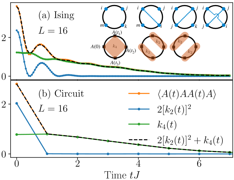
Figure 1: Multi-time correlation functions and ETH free-cumulants in chaotic systems. The full dynamics of $\langle A(t)AA(t)A\rangle$ (orange) is contrasted with the gaussian contribution $2[k_{2}(t)]^{2}$ (blue), the free cumulant $k_{4}(t)$ (green) and the sum of the two (dashed), cf. Eq.(4). (a) Ising model with $L=16$. (b) Floquet circuit with $L=14$. Inset: decomposition in non-crossing and crossing partitions of $\langle A(t_{1})A(t_{2})A(t_{3})A\rangle$ with $A_{ii}=0$. Top row: bookkeeping for the matrix elements $A_{ij}A_{jk}A_{km}A_{mi}$, the dashed line indicates an index contraction. Bottom row: non-crossing partitions in the dual partition and the associated free cumulants.

The high-order version of ETH was introduced in Ref.[38] to describe correlation functions between $q$ times. It predicts that the average of products of $q$ matrix elements with distinct indices is

$$\overline{A_{i_{1}i_{2}}A_{i_{2}i_{3}}\dots A_{i_{q}i_{1}}}=e^{-(q-1)S(E^{+})}F_{E^{+}}^{(q)}(\vec{\omega})\ ,$$ (1)

while products with repeated indices factorize in the large system size limit. Here, $e^{-S(E^{+})}$ is the mean level spacing at average energy $E^{+}=(E_{i_{1}}+\dots+E_{i_{q}})/q$, $\omega=(\omega_{i_{1}i_{2}},\dots,\omega_{i_{q-1}i_{q}})$ with $\omega_{ij}=E_{i}-E_{j}$ are $q-1$ energy differences and $F_{E^{+}}^{(q)}(\vec{\omega})$ is an order one smooth function of the energy density $E^{+}/N$ and $\vec{\omega}$, which encodes the physics. Throughout this paper, we will refer to Eq.(1) as general ETH . Building on this ansatz, Ref.[51] has recently argued that the building block of thermal multi-point correlation functions is given by free cumulants $k_{q}$, a type of connected correlation function defined in Free Probability (FP) [52]. These theoretical findings pinpoint the implications of the general ETH providing simple tools to determine correlation functions. However, to date, there has been no numerical investigation to test the general ETH in physically relevant many-body systems.

In this paper, we establish the validity of higher-order ETH (1) by numerical investigation of free cumulants in generic many-body systems with finite local Hilbert space and local interactions. We consider two archetypical classes of chaotic systems believed to model generic many-body quantum dynamics, non-integrable spin chains and Floquet brickwork circuits.

Using exact numerical methods, we demonstrate the ETH properties for four-point correlations at infinite temperature as a function of time and frequency. We show that the dynamics of four-point time correlation functions are encoded in the non-trivial behaviour of fourth-order free cumulant, see Fig. 1. This holds due to the exponential suppression of crossing diagrams and the factorization of non-crossing ones, as predicted by ETH in the FP description. To pinpoint the features of physical systems, we contrast ETH predictions with the results for rotationally invariant random matrices. The distinctive trait of Hamiltonian systems and unitary circuits is in the shape of the free cumulants $\tilde{k}_{4}(\vec{\omega})=F^{(4)}(\vec{\omega})$. Their non-trivial structure in frequency is the characteristic feature of ETH that distinguishes it from rotationally invariant random matrix theory. To the best of our knowledge, this is the first numerical evaluation of the frequency resolved higher-order ETH ansatz (1).

Free cumulants in ETH - The discussion of the consequences of the high-order ETH (1) is greatly simplified by applying the framework of FP [53; 52]. This is a branch of math with applications in random matrices [54] and combinatorics [55], that has recently appeared in many-body physics [51; 56]. Especially useful are the concepts of non-crossing partitions and free cumulants. Non-crossing partitions are partitions (decomposition of a set $\{1,\dots q\}$ in blocks) where the blocks do not “cross”. They enter in the combinatorial definition of free cumulants $k_{q}$ of order $q$ [52]: a specific type of connected correlation function, see [57] for a pedagogical introduction.

In Ref.[51] it was shown how to associate to each partition an ETH diagram corresponding to matrix elements restricted over specific indices. We consider for simplicity $q=4$, infinite temperature averages $\langle\bullet\rangle=\frac{\text{Tr}(\bullet)}{D}$ (where $D=\text{Tr}\,\mathbb{1}$ is the dimension of the Hilbert space) and observables $\hat{A}$ with $A_{ii}=0$, for the general treatment see [57]. Products $A_{ij}A_{jk}A_{km}A_{mi}$ are represented on a loop with four vertices/indices $i,j,k,m$, depicting energy eigenstates. The contractions between indices are represented by lines that connect the vertices, see the first line in Fig. 1a. Multi-time correlation functions $\langle A(t_{1})A(t_{2})A(t_{3})A(0)\rangle$ are then obtained by summing such products of matrix elements over all the indices. In this language, the ETH ansatz (1) reads: 1) crossing partitions are exponentially (in $\log D$) subleading with respect to the other terms

$$\frac{1}{D}\sum_{i\neq j}{|A_{ij}|^{4}}=\mathcal{O}(D^{-\alpha})\ ,\quad\alpha>0\ ,$$ (2)

and, 2) non-crossing partitions (also known as cactus diagrams [38]) factorize, e.g.

$$\begin{split}\frac{1}{D}&\sum_{i\neq j\neq m}e^{\mathrm{i}\omega_{ij}(t_{1}-t_{2})+i\omega_{im}t_{3}}{|A_{ij}|^{2}|A_{im}|^{2}}\\ &\quad\quad\simeq k_{2}(t_{1}-t_{2})k_{2}(t_{3})\ ,\end{split}$$ (3)

with $k_{2}(t)=\frac{1}{D}\sum_{i\neq j}|A_{ij}|^{2}e^{\mathrm{i}\omega_{ij}t}$. The result can be read diagrammatically on the dual of the non-crossing diagrams, where the new partition is identified via the observables on the links rather than on the vertices, see the second line in Fig.1a. These two conditions imply a simple structure for the multi-time correlators:

$$\begin{split}\langle A(t_{1})&A(t_{2})A(t_{3})A(0)\rangle=k_{4}(t_{1},t_{2},t_{3})\\ &\quad+k_{2}(t_{1}-t_{2})\,k_{2}(t_{3})+k_{2}(t_{2}-t_{3})\,k_{2}(t_{1})\ ,\end{split}$$ (4)

where the $k_{4}$ is given by the loop diagram (summations with all-different indices) as

$$\begin{split}k_{4}(\vec{t})&=\frac{1}{D}\sum_{i\neq j\neq m\neq k}A_{ij}A_{jk}A_{km}A_{mi}e^{i(\omega_{ij}t_{1}+\omega_{jk}t_{2}+\omega_{km}t_{3})}\end{split}$$ (5)

with $\vec{t}=(t_{1},t_{2},t_{3})$ and it corresponds to the fourth free cumulants that appear in FP [52]. Note that, in general, free cumulants are defined as a suitable connected correlation function, e.g. $k_{2}(AA)=\langle A^{2}\rangle-\langle A\rangle^{2}$ and $k_{4}(AAAA)=\langle A^{4}\rangle-2\langle A^{2}\rangle^{2}$ for $\langle A\rangle=0$. They can be identified with the summation over different indices [cf. below Eq.(3) and Eq. (5)] as a consequence of ETH. The free cumulant $k_{4}$ vanishes in the absence of correlations for $A_{nm}$ and hence it encodes the non-gaussian contributions in ETH. The ETH conditions (2)-(3) or equivalently the decomposition in Eq. (4) hold both in the time or the frequency domain. By standard ETH manipulations, for finite $\vec{\omega}=(\omega_{1},\omega_{2},\omega_{3})$, the Fourier transform of the free cumulants in Eq. (5) gives for generic $q$

$$\tilde{k}_{q}(\vec{\omega})=F^{(q)}(\vec{\omega})\ ,$$ (6)

and thus it yields all the physical properties as encoded in the smooth ETH functions of Eq. (1).

We note that non-trivial frequency dependence of free cumulants is the characteristic feature that distinguishes ETH from random matrix theory and not the absence of correlations. Generic rotationally invariant $D\times D$ random matrices are characterized by probability distribution of the elements $P(A)\equiv P(A_{ij})$ that is invariant under a change of basis:

$$P(A)=P(U^{\dagger}\,A\,U)\ ,$$ (7)

where $U$ may be an orthogonal, unitary, or symplectic random matrix ($UU^{\dagger}=U^{\dagger}U=\mathbb{1}$). A class with this property is given by matrix models $P(A)\propto\exp[-\frac{D}{2}\text{Tr}\,V(A)]$. In the case of the Gaussian ensembles, $V(A)=A^{2}/2$, while a general anharmonic (e.g. polynomial) potential $V(A)$ yields a statistically correlated matrix $A$. For rotationally invariant systems, Ref.[58] proved that the free cumulants are given by averages over simple loops (diagrams with different indices)

$$\,\overline{A_{i_{1}i_{2}}A_{i_{2}i_{3}}\dots A_{i_{q}i_{1}}}=D^{1-q}\,k_{q}(A)\ ,$$ (8)

where $k_{q}(A)$ is defined implicitly by cumulant-moment formula [52], see also Ref.[59]. Using the definition of the $q-$point spectral correlator ${R_{q}(\vec{\omega})=\sum_{i_{1}\neq i_{2}\neq\dots\neq i_{q}}\overline{\delta(\omega_{1}-\omega_{i_{1}i_{2}})...}\overline{\delta(\omega_{q-1}-\omega_{i_{q-1}i_{q}})}}$, the frequency-dependent free cumulants read (see [57])

$$\tilde{k}_{q}(\vec{\omega})=k_{q}(A)\frac{R_{q}(\vec{\omega})}{D^{q}}\simeq k_{q}(A)\ ,$$ (9)

where on the right-hand side we used $\frac{R_{q}(\vec{\omega})}{D^{q}}\simeq 1$ holding almost everywhere, i.e. when all frequencies $\omega_{ij}$ are much larger than mean level spacing [60]. Thus, the free cumulants in rotationally invariant random matrices are flat functions at finite frequencies. Eq. (9) represents a factorization into a term depending only on the statistics of the eigenvalues ${R_{q}(\vec{\omega})}/{D^{q}}$ and a constant depending only on the observable $A$. This has been referred to as spectral decoupling [61] and is a consequence of rotational invariance.

Models - As a paradigmatic example of chaotic non-integrable Hamiltonian, we consider the Ising chain with transverse and longitudinal fields described by the Hamiltonian

$$\hat{H}=\sum_{i=1}^{L}w\hat{\sigma}_{i}^{x}+\sum_{i=1}^{L}h\hat{\sigma}_{i}^{z}+\sum_{i=1}^{L}J\hat{\sigma}_{i}^{z}\hat{\sigma}_{i+1}^{z}\ ,$$ (10)

where $\hat{\sigma}^{\alpha}_{i}$ is a Pauli matrix on site $i$ in the direction $\alpha=x,y,z$. We measure time in units of $J$ and set $w=\sqrt{5}/2$, $h=(\sqrt{5}+5)/8$. With periodic boundary conditions, this system has translation and space reflection symmetries. We consider the reflection-even symmetry subsector corresponding to fixed $k=0$ quasi-momentum. We focus on the extensive operator

$$\hat{A}=\frac{1}{\sqrt{L}}\sum_{i=1}^{L}\hat{\sigma}_{i}^{y}\ ,$$ (11)

that enjoys the property $A_{nn}=0$, since $\hat{A}=[\hat{H},\hat{A}^{\prime}]$ with $\hat{A}^{\prime}\propto\sum_{i}\hat{\sigma}_{i}^{z}$. The results hold also for the magnetization along $x$ and $z$, as well as for local operators, see [57].

As a representative of chaotic Floquet evolution, we consider a brick-wall circuit design on a qubit chain of even length $L$ and periodic boundary conditions. These models have attracted much attention recently, as they can be used to model discrete-time evolution in quantum computation and provide unique analytical insights [62; 63; 64; 65]. The system undergoes discrete-time evolution governed by the unitary Floquet operator $\mathcal{U}$ with eigenvalues $e^{-\mathrm{i}\phi_{n}}$, defining quasi-energy spectrum $\{\phi_{n}\}\subset[0,2\pi)$ stepping in place of $\{E_{n}\}$. Each time step is composed of two half-time steps such that $\mathcal{U}=\mathcal{U}_{2}\mathcal{U}_{1}$ with

$$\mathcal{U}_{1}=U_{1}^{\otimes L/2}\ ,\quad\mathcal{U}_{2}=\mathcal{T}\,U_{2}^{\otimes L/2}\mathcal{T}^{-1},$$ (12)

where $\mathcal{T}$ denotes a periodic shift on the lattice by one site. We show results for generic unitary two-qubit gates $U_{1}$ and $U_{2}$ (see [57]), with $U_{1}\neq U_{2}$ to avoid undesired symmetries. The circuit lacks symmetry under spatial reflection, so we restrict ourselves to the full $k=0$ quasi-momentum subsector. We fix a pair of randomly chosen gates but ensure that they are representative of generic gates. We did all the calculations also for dual-unitary gates, which were recently introduced as exactly solvable models of chaotic circuit dynamics [62], for which we obtain the same results. However, their defining space-time duality is not sufficient to allow for exact evaluation of the high-order ETH predictions and we hence report the result on generic gates only. Following the two-site shift-invariance of $\mathcal{U}$, we now consider an extensive operator

$$\hat{A}=\sqrt{\frac{2}{L}}\sum_{i=0}^{L/2-1}\hat{\sigma}_{2i+1}^{z}$$ (13)

acting on the odd sublattice only. Here, we manually set the diagonal entries to zero, which qualitatively does not change the results as it amounts only to a constant shift in the correlators. The factor $\sqrt{L}$ and $\sqrt{L/2}$ in Eq. (11) and Eq. (13) is chosen to ensure normalization $\langle\hat{A}^{2}\rangle=1$.

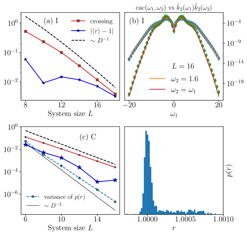
Figure 2: High-order ETH conditions (2)-(3) as a function of the system size $L$ in the Ising model (a) and the Unitary Circuit (c). We denote with “crossing” Eq.(2), while $r$ corresponds to Eq.(14). (b) Ising model factorization: the non-crossing contribution $\text{cac}(\omega_{1},\omega_{2})$ (full line) in (3) is compared with the factorized result $\tilde{k}_{2}(\omega_{1})\tilde{k}_{2}(\omega_{2})$ (diamonds) in the frequency domain, along two directions $\omega_{2}=1.6$ and $\omega_{2}=\omega_{1}$ for $L=16$. (d) Distribution of the ratio $r$ (16) with $\omega_{1}\neq\omega_{2}$ in the circuit for $L=14$. The variance of this distribution as a function of $L$ is plotted in panel (c).

Results - We perform full diagonalization of $\hat{H}$ for the Ising model and $\mathcal{U}$ for the Circuit and test the general ETH ansatz by studying the statistics of $A_{nm}=\langle n|\hat{A}|m\rangle$ as a function of the energy $\omega_{nm}=E_{n}-E_{m}$ and the eigenphase differences $\omega_{nm}=\phi_{n}-\phi_{m}$, respectively. Here we discuss the data for $\hat{A}$ a collective observable. The same results for local operators are shown in [57]. First, we look at the exponential suppression of crossing partitions [cf. Eq. (2)] and at the factorization of non-crossing parts [cf. Eq. (3)]. The contribution of the crossing partition (2) as a function of the system size $L$ is shown in Fig.2a,c for the Ising and Circuit models, respectively. Both cases show an exponential suppression with $L$, as the crossing contribution decreases with the inverse of the Hilbert space dimension $\sim D^{-1}$. Then, we check the factorization of the non-crossing partitions [cf. Eq. (3)]. To study it as a function of $L$, we consider the ratio

$$\langle r\rangle=\frac{\text{cactus}(0,0)}{[k_{2}(0)]^{2}}\ ,$$ (14)

where we defined

$$\text{cactus}(t_{1},t_{2})=\frac{1}{D}\sum_{i\neq j\neq m}e^{\mathrm{i}\omega_{ij}t_{1}+i\omega_{im}t_{2}}{|A_{ij}|^{2}|A_{im}|^{2}}$$ (15)

as the left-hand side of Eq. (3). The general ETH predicts that the ratio converges to one in the limit ${L\to\infty}$. This is shown in Fig. 2a,c, where we plot $|\langle r\rangle-1|$ for the Ising and the Circuit model, respectively. From the data of the Ising model, one can not infer the exact scaling with the system size. However, we note that the absolute values of $|\langle r\rangle-1|$ for the Circuit are at least one order of magnitude smaller than in the Hamiltonian case. This factorization holds also in the frequency domain, as shown in Fig. 2b,d. In panel b, we plot the Fourier transform of Eq. (15), i.e.

$$\text{cac}(\omega_{1},\omega_{2})\!\! = \!\!\!\frac{1}{D}\!\!\!\sum_{i\neq j\neq m}\!\!\!\delta_{\tau}(\omega_{1}\!-\!\omega_{ij})\delta_{\tau}(\omega_{2}\!-\!\omega_{im}){|A_{ij}|^{2}|A_{im}|^{2}}$$

and the product $\tilde{k}_{2}(\omega_{1})\tilde{k}_{2}(\omega_{2})$ along two directions $\omega_{2}=\omega_{1}$ and $\omega_{2}=1.6$ for the Ising model with $L=16$. Here we indicate with $\delta_{\tau}(\omega)$ a smoothed delta function of width $1/\tau$, such that $\lim_{\tau\to\infty}\delta_{\tau}(\omega)=\delta(\omega)$. We choose a Gaussian function $\delta_{\tau}(\omega)=\frac{\tau}{\sqrt{2\pi}}e^{-\tau^{2}\omega^{2}/2}$, fixing $\tau\gg 1$ such that the results no longer depend on it ($\tau=2.5$ for the Ising model and $\tau=10$ for the circuit). The data show a good agreement between the two predictions. In panel d, we consider the Floquet circuit evolution and we show the distribution of the frequency-dependent ratio

$$r(\omega_{1},\omega_{2}) = \frac{{\text{cac}}(\omega_{1},\omega_{2})}{\tilde{k}_{2}(\omega_{1})\tilde{k}_{2}(\omega_{2})}\ ,$$ (16)

for $L=14$ with $\omega_{1}\neq\omega_{2}$. The probability density $p(r)$ peaks at one, with a small variance that decreases with the system size with a double exponential $\sim D^{-2}$, as evidenced in Fig. 2c. The factorization of the non-crossing contributions holds also as a function of time, see [57].

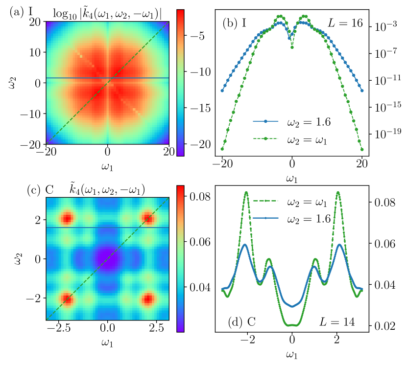
Figure 3: Frequency dependence of the fourth free cumulant $\tilde{k}_{4}(\omega_{1},\omega_{2},-\omega_{1})$ for the Ising model, with $L=16$ and $\tau=2.5$ (ab) and the Floquet circuit with $L=12$ and $\tau=10$ (cd). On the right (b,d), the frequency dependence is plotted along two directions $\omega_{1}=\omega_{2}$ (green) and $\omega_{2}=1.6$ (blue).

The exponential suppression of crossing partitions and factorization of non-crossing ones lead to the decomposition of multi-point correlations given by Eq. (4). We test it by looking at the out-of-time order correlator (OTOC) $\langle A(t)\,A\,A(t)\,A\rangle$ for which the free-cumulant decomposition reads

$$\langle A(t)AA(t)A\rangle\simeq 2[k_{2}(t)]^{2}+k_{4}(t)$$ (17)

where $k_{4}(t)$ is given by Eq. (5) with $t_{1}=t_{3}=t$ and $t_{2}=0$. The numerical results for the Ising and circuit models are presented in Fig. 1a,b for $L=16$ and $L=14$, respectively. The dynamics of $\langle A(t)AA(t)A\rangle$ is compared with the Gaussian (Wick) contribution $2[k_{2}(t)]^{2}$, the fourth free cumulant $k_{4}(t)$, and the sum of two [cf. Eq. (17)] which shall give the full result. The remarkable agreement for both classes of many-body evolution is one of the main results of the paper. After a short time, the two-point correlation $k_{2}(t)$ approaches zero, while the OTOC displays slower dynamics, which is in turn well captured by $k_{4}(t)$. This shows that all non-trivial information about four-point functions is encoded in the fourth free cumulant $k_{4}(t)$ which thus quantifies OTOC dynamics at longer time scales.

To characterize such higher-order correlations, we finally study the fourth free cumulant (5) in frequency:

$$\tilde{k}_{4}(\omega_{1},\omega_{2},\omega_{3}) =\frac{1}{D}\sum_{i\neq j\neq m\neq k}A_{ij}A_{jk}A_{km}A_{mi}$$ (18)

$$\times\delta_{\tau}(\omega_{ij}-\omega_{1})\delta_{\tau}(\omega_{jk}-\omega_{2})\delta_{\tau}(\omega_{km}-\omega_{3})\ .$$

The results are shown in Fig. 3 for $\omega_{3}=-\omega_{1}$. In panels (b) and (d) we plot the behaviour along two directions $\omega_{2}=\omega_{1}$ and $\omega_{2}=1.6$, for the Ising Hamiltonian and circuit respectively. Both classes display a clear frequency dependence of the fourth free cumulant $\tilde{k}_{4}(\vec{\omega})$. While in the Hamiltonian case $\tilde{k}_{4}(\vec{\omega})$ rapidly decays at large frequencies (Fig. 3ab), in the Floquet evolution frequencies have a period of $2\pi$ and the non-trivial dynamics is restricted to this interval (Fig. 3c,d). This behaviour is thus in stark contrast with the result for random matrices (for which free cumulants are a flat function of frequency) [cf. Eq. (9)] and is the distinguishing feature of ETH for physical many-body lattice systems.

Discussion and conclusions - Our work illustrates that the general framework of ETH applies to non-integrable interacting lattice models. General (higher-order) ETH implies that the correlation functions of physical systems are characterized by: (i) suppression of crossing contributions, (ii) factorization of non-crossing ones, and (iii) non-trivial behaviour of free cumulants $k_{q}$. The same results should be expected at finite temperatures (or energy density), whose precise system size scaling is left to future investigations.

Let us remark that dual-unitary Floquet circuits, representing a paradigm of maximally chaotic dynamics with local interactions [62], display qualitatively exactly the same phenomenology. In particular, free cumulants depend on frequency, as already established for the second cumulant $\tilde{k}_{2}(\omega)$ in Ref.[22]. This behaviour differs from the structureless random matrix result of Ref.[66] (cf. Eq. (9)) derived for locally interacting systems in the limit of infinite local Hilbert space dimension $d\to\infty$. Even though for finite $d$, dual-unitarity allows for analytically tractable results in the thermodynamic limit [62], establishing rigorous results in the context of ETH remains a challenging problem as it requires precise control of finite size corrections. For instance, even if time-order correlators can be understood via a channel approach, the dynamics of OTOC at finite times can be solved exactly only on the light cone [64]. Thus, it remains an open question whether one can obtain some analytical understanding of higher-order free cumulants for any type of finite $d$ models with local interactions.

Our findings can be used as a starting point for further investigations. The behaviour of $k_{4}(t)$ for the Ising model and the Floquet circuit is similar at long times (Fig. 1) and it is suggestive of some form of universality. Such dynamical results indicate a hierarchy of correlation functions at different orders, $k_{2},k_{4}$, etc, which should be of interest to explore systematically.

Potential insights could be achieved by probing the higher-order ETH conditions Eqs. (2),(3) or Eq. (4) in the presence of integrability – for which ETH is a highly debated open issue [67; 68; 69] – but this is left for future research.

——————————

Supplemental Material:

In this Supplementary Material, we provide additional analysis and background calculations to support the results in the main text. In Sec.1, we provide the theoretical background to understand free cumulants, we exemplify their role in ETH and for rotationally invariant random matrices. In Sec.2 we analyze the factorization of the cactus diagram in the time domain. In Sec.3 we report the same results illustrated in the main text in the case of different operators.

1 Introduction to Free Cumulants and their expression in ETH

In this Appendix, we provide a self-contained and pedagogical introduction to the definition of free cumulants, starting from the combinatorial approaches to classical cumulants. Then, we review their use to understand the general ETH Eigenstate Thermalization Hypothesis and finally discuss their behaviour in rotationally invariant systems.

1.1 Classical Cumulants

Let us denote with “classical cumulants” the standard cumulants of commuting random variables. Consider $x$ a random variable with probability $p(x)$ and average $\mathbb{E}(\bullet)=\int\bullet p(x)dx$. Classical cumulants $c_{n}(x)$ are defined as connected correlation functions: a suitable combination of moments $m_{n}=\mathbb{E}(x^{m})$ of the same or lower order. For instance, the first four orders read

$$c_{1}(x) =\mathbb{E}(x)$$ (S1a)

$$c_{2}(x) =\mathbb{E}(x^{2})-\mathbb{E}(x)^{2}$$ (S1b)

$$c_{3}(x) =\mathbb{E}(x^{3})-3\mathbb{E}(x^{2})\mathbb{E}(x)+2\mathbb{E}(x)^{3}$$ (S1c)

$$c_{4}(x) =\mathbb{E}(x^{4})-3\mathbb{E}(x^{2})^{2}-4\mathbb{E}(x)\mathbb{E}(x^{3})+12\mathbb{E}(x^{2})\mathbb{E}(x)^{2}-6\mathbb{E}(x)^{4}\ .$$ (S1d)

Notably, the specific coefficients appearing in this expression can be obtained in a combinatorial way, based on the concept of partitions. A partition $\pi$ of a set $\{1,\dots n\}$ is a decomposition in blocks that do not overlap and whose union is the whole set. The set of all partitions of $\{1,2,\dots n\}$ is denoted $P(n)$. The example of $P(4)$ for $\{1,2,3,4\}$ is shown in Fig.S1, where with $\times[m]$ we denote that there are $m$ cyclic permutations. The number of the partitions of a set with $n$ elements is called the Bell number $B_{n}$ defined recursively as $B_{n+1}=\sum_{k=0}^{n}\binom{n}{k}B_{k}$ with $B_{1}=1$ and $B_{2}=2$, $B_{3}=5$, $B_{4}=15$, $B_{5}=52$, etc. The classical cumulants (S1) can be defined implicitly by the moments/classical cumulants formula from the sum over all possible partitions

$$\mathbb{E}(x^{n})=\sum_{\pi\in P(n)}c_{\pi}(x)\quad\quad\text{with}\quad c_{\pi}(x)=\prod_{b\in\pi}c_{|b|}(x)\ ,$$ (S2)

where on the right-hand side $|b|$ denotes the number of elements of the block $b$ of the partition $\pi$. The result for the first four orders reads

$$\mathbb{E}(x) =c_{1}(x)$$ (S3a)

$$\mathbb{E}(x^{2}) =c_{2}(x)+c_{1}^{2}(x)$$ (S3b)

$$\mathbb{E}(x^{3}) =c_{3}(x)+3c_{2}(x)c_{1}(x)+c_{1}^{3}(x)$$ (S3c)

$$\mathbb{E}(x^{4}) =c_{4}(x)+3c_{2}^{2}(x)+4c_{2}(x)c_{1}^{2}(x)+4c_{3}(x)c_{1}(x)+c_{1}^{4}(x)\ .$$ (S3d)

Note that the coefficients correspond exactly to the multiplicities of each diagram. By inverting these relations one immediately finds the classical cumulants in Eq.(S1).

Here we only reported the definition for a single random variable, but the same can be easily extended to families of random variables $(x_{1},x_{2},\dots)$ from

$$\mathbb{E}(x_{1}x_{2}\dots x_{n})=\sum_{\pi\in P(n)}c_{\pi}(x_{1}x_{2}\dots x_{n})\quad\text{with}\quad c_{\pi}(x_{1}x_{2}\dots x_{n})=\prod_{b\in\pi}c_{|b|}(x_{b(1)}x_{b(2)}\dots x_{b(n)})\ ,$$ (S4)

where $b=(b(1),b(2),\dots,b(n))$ denotes the element of the block of the partition.

Summarizing, classical cumulants are connected correlation functions, whose coefficients can be computed from the combinatorial counting of partitions. A crucial property of Gaussian distributions is that cumulants of order greater than two vanish. Hence classical cumulants can be thought of as the connected correlations such that $c_{n>2}=0$ for Gaussian random variables.

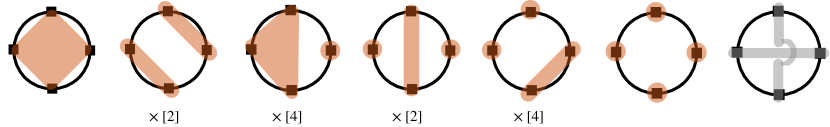
Figure S1: Set of all partitions for $n=4$. With the colour orange, we represent the non-crossing partitions, while the crossing one is in grey. With $\times[m]$, we denote the $m$ cyclic permutations of that partition, which determines the coefficients appearing in the moment/cumulant formulas in Eq.(S1) and Eq.(S9).

1.2 Free cumulants

We are now in the position to define free cumulants, which generalize the previous definition to non-commuting variables. For definiteness, let us start by considering a $D\times D$ random matrix $A$ and the so-called “expectation value”

$$\phi(\bullet)=\lim_{D\to\infty}\frac{1}{D}\mathbb{E}\left[\mathrm{Tr}(\bullet)\right]\ ,$$ (S5)

which is well defined in the large $D$ limit and normalized, i.e. $\phi(\mathbb{1})=1$.

The definition of free cumulants is based on the combinatorics of non-crossing partitions, which are partitions that do not cross. The set of non-crossing partitions of $\{1,2,\dots n\}$ is denoted by $NC(n)$ and enumerated by Catalan numbers $C_{n}=(1+1/n)\binom{2n}{n}$ with $C_{1}=1$, $C_{2}=2$, $C_{3}=5$, $C_{4}=14$, $C_{5}=42$, etc. Hence the number of crossing and non-crossing partitions differs from $n=4$ on, as shown in Fig.S1. Free cumulants $k_{n}(A)$ are hence defined implicitly by

$$\phi(A^{n})=\sum_{\pi\in NC(n)}k_{\pi}(A)\quad\text{with}\quad k_{\pi}(A)=\prod_{b\in\pi}k_{|b|}(A)\ ,$$ (S6)

where we recall that $|b|$ is the size of each block in the partition $\pi$. This expression for the first few orders reads

$$\phi(A) =k_{1}(A)$$ (S7a)

$$\phi(A^{2}) =k_{2}(A)+k_{1}(A)^{2}$$ (S7b)

$$\phi(A^{3}) =k_{3}(A)+3k_{2}(A)k_{1}(A)+k_{1}(A)^{3}$$ (S7c)

$$\phi(A^{4}) =k_{4}(A)+3k_{2}(A)^{2}+4k_{2}(A)k_{1}(A)^{2}+4k_{3}(A)k_{1}(A)+k_{1}(A)^{4}\ ,$$ (S7d)

which, by inverting for $k_{n}$ leads to

$$k_{1}(A) =\phi(A)\ ,$$ (S8a)

$$k_{2}(A) =\phi(A^{2})-\phi(A)^{2}\ ,$$ (S8b)

$$k_{3}(A) =\phi(A)^{3}-3\phi(A^{2})\phi(A)+2\phi(A)^{3}\ ,$$ (S8c)

$$k_{4}(A) =\phi(A^{4})-2\phi(A^{2})^{2}-4\phi(A)\phi(A^{3})+10\phi(A^{2})\phi(A)^{2}-5\phi(A)^{4}\ .$$ (S8d)

The first difference between classical and free cumulants appears in the fourth order, as one notices by comparing the factor $2\times\phi(A^{2})^{2}$ in Eq.(S7) instead of the $3\times\mathbb{E}(x^{2})^{2}$ in Eq.(S3).

For Gaussian random matrices, the free cumulants of order greater than two vanish. It is now clear that free cumulants are the direct generalization of classical cumulants to non-commuting objects and that they can be thought of as the connected correlations such that $k_{n>2}=0$ for Gaussian random matrices.

The definition of free cumulants can be immediately extended to different random matrices $(A^{(1)},A^{(2)},...)$ as

$$\phi(A^{(1)}A^{(2)}...A^{(n)})=\sum_{\pi\in NC(n)}k_{\pi}(A^{(1)}A^{(2)}...A^{(n)})\quad\text{with}\quad k_{\pi}(A^{(1)}A^{(2)}...A^{(n)})=\prod_{b\in\pi}k_{|b|}(A^{(b(1))}A^{(b(2))}...A^{(b(n))})\ ,$$ (S9)

where $b=(b(1),b(2),\dots,b(n))$ denotes the element of the block of the partition. As an example, consider the following partition $\pi$ for $n=8$:

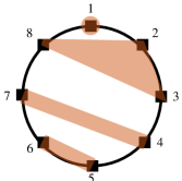
Figure S2: A non-crossing partition $\pi$ of $n=8$.

Here the blocks are $\{\{1\},\{2,3,8\},\{4,7\},\{5,6\}\}$ and the corresponding contribution reads:

$$k_{\pi}(A^{(1)}...A^{(8)})=k_{1}(A^{(1)})k_{3}(A^{(2)}A^{(3)}A^{(8)})k_{2}(A^{(4)}A^{(7)})k_{2}(A^{(5)}A^{(6)})\ .$$ (S10)

By inverting the implicit definition in Eq.(S9), the first few free cumulants read

$$k_{1}(A^{(1)}) =\phi(A^{(1)})\ ,$$ (S11a)

$$k_{2}(A^{(1)}A^{(2)}) =\phi(A^{(1)}A^{(2)})-\phi(A^{(1)})\phi(A^{(2)})\ ,$$ (S11b)

$$\begin{split}k_{3}(A^{(1)}A^{(2)}A^{(3)})&=\phi(A^{(1)}A^{(2)}A^{(3)})-\phi(A^{(1)}A^{(2)})\phi(A^{(3)})-\phi(A^{(1)}A^{(3)})\phi(A^{(3)})-\phi(A^{(2)}A^{(3)})\phi(A^{(1)})\\ &\quad+2\phi(A^{(1)})\phi(A^{(2)})\phi(A^{(3)})\ .\end{split}$$ (S11c)

1.3 General ETH and Free cumulants

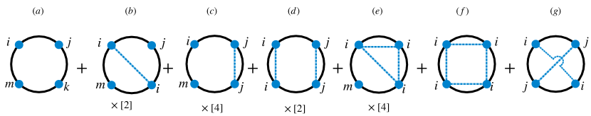
Figure S3: Bookeeping of ETH matrix elements for $n=4$. Matrix elements $A_{ij}$ lie on the vertex connecting two dots, which represent the energy index. Blue dots represent different indices and the edges connecting two or more dots represents a contraction among them.

In this Appendix, we review the Free Probability approach to the general ETH ansatz as discussed in Ref.[51].

First of all, revisiting the definition (S9), one can define thermal free cumulants $k^{\beta}_{q}$ by

$$\langle A(t_{1})A(t_{2})\dots A(t_{q})\rangle_{\beta}=\sum_{\pi\in NC(q)}k^{\beta}_{\pi}\left(A(t_{1})A(t_{2})\dots A(t_{q})\right)\ ,$$ (S12)

where $\langle\bullet\rangle_{\beta}=\frac{1}{Z}\mathrm{Tr}\left(e^{-\beta H}\bullet\right)$ with $Z=\mathrm{Tr}\left(e^{-\beta H}\right)$ plays the role of the expectation value $\phi()$. Here $k^{\beta}_{\pi}$ are products of thermal free cumulants one for each block of $\pi$, i.e.

$$k^{\beta}_{\pi}\left(A(t_{1})A(t_{2})\dots A(t_{q})\right)=\prod_{b\in\pi}k^{\beta}_{|b|}(\prod_{j\in b}A(t_{j}))\ ,$$ (S13)

where $|b|$ is the size of the block $b$ in the partition $\pi$ See the example in Fig.S2, where now $t_{j}$ is playing the role of the index $j$. Exactly as in Eq.(S9), this is just an implicit definition of cumulants in terms of moments, which can be defined in principle also for integrable or non-ergodic systems. We will now discuss how this definition simplifies the discussion of the general ETH which, in turn, implies a particularly simple form for the thermal free cumulants.

The general version of the Eigenstate-Thermalization-Hypothesis has been introduced by Ref.[38] as an ansatz on the statistical properties of the product of $q$ matrix elements $A_{ij}$. Specifically, the average of products with distinct indices $i_{1}\neq i_{2}\dots\neq i_{q}$ reads

$$\overline{A_{i_{1}i_{2}}A_{i_{2}i_{3}}\dots A_{i_{q}i_{1}}}=e^{-(q-1)S(E^{+})}F_{e^{+}}^{(q)}(\omega_{i_{1}i_{2}},\dots,\omega_{i_{q-1}i_{q}})$$ (S14a)

while, with repeated indices, it shall factorize in the large $$N$$ limit as

$$\overline{A_{i_{1}i_{2}}\dots A_{i_{k-1}i_{1}}A_{i_{1}i_{k+1}}\dots A_{i_{q}i_{1}}}=\overline{A_{i_{1}i_{2}}\dots A_{i_{k-1}i_{1}}}\;\overline{A_{i_{1}i_{k+1}}\dots A_{i_{q}i_{1}}}\ .$$ (S14b)

In Eq.(S14a), $Ne^{+}=E^{+}=(E_{i_{1}}+\dots+E_{i_{q}})/q$ is the average energy, $\vec{\omega}=(\omega_{i_{1}i_{2}},\dots,\omega_{i_{q-1}i_{q}})$ with $\omega_{ij}=E_{i}-E_{j}$ are $q-1$ energy differences and $F_{e^{+}}^{(q)}(\vec{\omega})$ is a smooth function of the energy density $e^{+}=E^{+}/N$ and $\vec{\omega}$. Thanks to the explicit entropic factor, the functions $F^{(q)}_{E}(\vec{\omega})$ are of order one and they contain all the physical information.

One would like to understand how this ansatz applies to multi-time correlation functions as

$$\langle A(t_{1})A(t_{2})\dots A(t_{q})\rangle_{\beta}\ .$$ (S15)

The full result is given by the sum over all indices of ${A_{i_{1}i_{2}}A_{i_{2}i_{3}}\dots A_{i_{q}i_{1}}}$. Thus, to determine the contribution of the different matrix elements one shall consider all the possible contractions. One can do this diagrammatically. Let us consider the example of four-point functions that we illustrate pictorially in Fig.S3. Products $A_{ij}A_{jk}A_{km}A_{mi}$ are represented on a loop with four vertices $i,j,k,m$, depicting energy eigenstates. The contractions between two or more indices are represented by lines that connect the vertices. The blue dots indicate that the indices are all different. For instance, the first diagram represents $A_{ij}A_{jk}A_{km}A_{mi}$, the second $A_{ij}A_{ji}A_{im}A_{mi}$, the third $A_{ij}A_{jj}A_{jm}A_{mi}$ with all distinct indices, and so on. One recognizes that there are two types of diagrams: (1) non-crossing ones – in which the polygons created by the indices do not cross (the simple loops with all different indices are in this class) – and (2) crossing ones, in which the lines cross. The general ETH ansatz in Eqs.(LABEL:GEN_ETH) implies

1. all non-crossing diagrams yield a finite contribution with factorization of non-crossing diagrams into products of irreducible simple loops:

   $$\frac{1}{Z}\sum_{i\neq j\neq m}e^{-\beta E_{ii}}e^{\mathrm{i}\omega_{ij}(t_{1}-t_{2})+i\omega_{im}t_{3}}{|A_{ij}|^{2}|A_{im}|^{2}}\simeq\left(\frac{1}{Z}\sum_{i\neq j}e^{-\beta E_{ii}}e^{-i\omega_{ij}(t_{1}-t_{2})}|A_{ij}|^{2}\right)\left(\frac{1}{Z}\sum_{i\neq m}e^{-\beta E_{ii}}e^{-i\omega_{im}t_{3}}|A_{im}|^{2}\right)\ .$$ (S16)

   which means that the diagrams (b-f) in Fig.S3 can be cut along the blue line.

2. crossing diagrams are suppressed with the inverse of the density of states as

   $$\frac{1}{Z}\sum_{i\neq j}e^{-\beta E_{ii}}e^{\mathrm{i}\omega_{ij}(t_{1}-t_{2}+t_{3})}{|A_{ij}|^{4}}\simeq e^{-S(E)}\sim D^{-1}\ ,$$ (S17)

   which means that they can be neglected for the purpose of computing higher-order correlation functions.

The correspondence with Free Probability allows one to generalize the result at every $k$. First of all, all the contribution to multi-time correlations has to be found in non-crossing partitions. Specifically, the non-crossing ETH diagrams ((a-f) in Fig.S3) can be read as the “dual” of non-crossing partitions $\pi$ in which every element of the set is not associated with an observable [(a-f) in Fig.S1]. Secondly, the ETH factorization implies a particularly simple form for the $k^{\beta}_{q}$ defined in Eq.(S12). Namely, the thermal free cumulants of ETH-obeying systems are given only by summations with distinct indices

$$k^{\rm ETH}_{q}\left(A(t_{1})A(t_{2})\dots A(t_{q})\right) =\frac{1}{Z}\sum_{i_{1}\neq i_{2}\neq\dots\neq i_{q}}e^{-\beta E_{i}}A_{i_{1}i_{2}}A_{i_{2}i_{3}}\dots A_{i_{q}i_{1}}e^{it_{1}\omega_{i_{1}i_{2}}+\dots it_{q}\omega_{i_{q}i_{1}}}$$ (S18)

$$=\text{FT}\left[F^{(q)}_{e_{\beta}}(\vec{\omega})e^{-\beta\vec{\omega}\cdot\vec{\ell}_{q}}\right]\ ,$$ (S19)

where in the second line $\text{FT}[\bullet]=\int d\vec{\omega}e^{i\vec{\omega}\cdot\vec{t}}\bullet$ is the Fourier transform and $e_{\beta}=\langle H\rangle_{\beta}/N$ is the thermal energy density. The thermal weight with $\vec{\ell}_{q}=\left(\frac{q-1}{q},\dots,\frac{1}{q},0\right)$ corresponds to a generalization of the fluctuation-dissipation theorem. This result shows that all the correlations of the general ETH (1) are encoded precisely in the thermal free cumulants. On four-point functions, the validity of the ETH ansatz implies:

$$\begin{split}\langle A(t_{1})A(t_{2})A(t_{3})A(t_{4})\rangle_{\beta}=&k_{4}^{\rm ETH}(t_{1},t_{2},t_{3},t_{4})+k_{2}^{\rm ETH}(t_{1},t_{2})k^{\rm ETH}_{2}(t_{3},t_{4})+k_{2}^{\rm ETH}(t_{1},t_{4})k^{\rm ETH}_{2}(t_{2},t_{3})\\ &+k^{\rm ETH}_{1}\Big{[}k^{\rm ETH}_{3}(t_{1},t_{2},t_{3})+k^{\rm ETH}_{3}(t_{1},t_{3},t_{4})+k^{\rm ETH}_{3}(t_{1},t_{2},t_{4})+k^{\rm ETH}_{3}(t_{2},t_{3},t_{4})\\ &\quad\quad+k^{\rm ETH}_{1}k^{\rm ETH}_{2}(t_{1},t_{3})+k^{\rm ETH}_{1}k^{\rm ETH}_{2}(t_{2},t_{4})+(k^{\rm ETH}_{1})^{3}\\ &\quad\quad+k^{\rm ETH}_{1}k^{\rm ETH}_{2}(t_{1},t_{2})+k^{\rm ETH}_{1}k^{\rm ETH}_{2}(t_{1},t_{4})+k^{\rm ETH}_{1}k^{\rm ETH}_{2}(t_{2}t_{3})+k^{\rm ETH}_{1}k^{\rm ETH}_{2}(t_{3},t_{4})\Big{]}\ .\end{split}$$ (S20)

For $k_{1}=0$, this expression reduces to Eq.(4) of the main text, where we make explicit use of time-translational invariance, i.e. $k_{q}(t_{1},t_{2},...t_{q})=k_{q}(t_{1}-t_{q},t_{2}-t_{q},...,t_{q-1}-t_{q})$.

1.4 Free cumulants in rotationally invariant systems

In this Appendix, we derive the result in Eq.(9) of the main text.

Rotationally invariant models are characterized by probability distribution of the matrix elements $P(A)\equiv P(A_{ij})$ that is invariant under a change of basis:

$$P(A)=P(U^{\dagger}\,A\,U)\ ,$$ (S21)

where $U$ may be an orthogonal, unitary, or symplectic matrix ($UU^{\dagger}=U^{\dagger}U=\mathbb{1}$). Let us denote $\overline{\bullet}$ averages over these ensembles. A class which enjoys this property is given by $P(A)\propto\exp[-\frac{D}{2}\text{Tr}V(A)]$ where $V(A)$ is a generic polynomial - the potential ($V(A)=A^{2}/2$ in the case of the Gaussian ensemble). These matrices have the property that their moments only depend on the distributions of the eigenvalues $a_{i}$, i.e. $\langle A^{m}\rangle=\frac{1}{D}\mathrm{Tr}(A^{m})=\frac{1}{D}\sum_{i}a_{i}^{m}$.

For rotationally invariant systems, Ref. [58] proved that the free cumulants are given by averages over simple loops (diagrams with different indices)

$$\,\overline{A_{i_{1}i_{2}}A_{i_{2}i_{3}}\dots A_{i_{q}i_{1}}}=D^{1-q}\,k_{q}(A)\quad\text{with}\quad i_{1}\neq\dots\neq i_{q}$$ (S22)

at the leading order in $D$. Here the average is taken according to $P(A)$ in Eq. (S21) and $k_{q}(A)$ is defined in Eq. (S6). The equality holds for each product of matrix elements, without the summation [in contrast with Eq. (5) of the main text]. The overall constant normalization $D^{q-1}$ stands for the fact that the average over each element is the same. For $q=2$ this equation reads

$$\overline{A_{ij}A_{ji}}=D^{-1}\,k_{2}(A)=D^{-1}\,\left(\,\langle A^{2}\rangle-\langle A\rangle^{2}\,\right)\ ,$$ (S23)

where $k_{2}(A)$ is given in Eq. (S8b). This result corresponds to the ETH ansatz for $q=2$ for GUE (CUE) matrices.

We now compute free cumulants in the frequency domain

$$\tilde{k}_{q}(\omega_{1},\omega_{2},\dots,\omega_{q-1})=\frac{1}{D}\sum_{i_{1}\neq i_{2}\neq\dots\neq i_{q}}\overline{A_{i_{1}i_{2}}A_{i_{2}i_{3}}\dots A_{i_{q}i_{1}}\delta(\omega_{1}-(E_{i_{1}}-E_{i_{2}}))\dots\delta(\omega_{q-1}-(E_{i_{q-1}}-E_{i_{q}}))}\ .$$ (S24)

We assume a decoupling between the average over ${A_{i_{1}i_{2}}A_{i_{2}i_{3}}\dots A_{i_{q}i_{1}}}$ and the average over the delta functions (absence of statistical correlation between matrix elements and the spectrum) . Substituting Eq. (S22) into Eq. (S24) we thus conclude

$$\tilde{k}_{q}(\omega_{1},\omega_{2},\dots,\omega_{q-1})=k_{q}(A)\frac{R_{q}(\omega_{1},\omega_{2},\dots\omega_{q-1})}{D^{q}}\ ,$$ (S25)

where

$$R_{q}(\omega_{1},\omega_{2},\dots\omega_{q-1})=\sum_{i_{1}\neq i_{2}\neq\dots\neq i_{q}}\overline{\delta(\omega_{1}-(E_{i_{1}}-E_{i_{2}}))\delta(\omega_{2}-(E_{i_{2}}-E_{i_{3}}))\dots\delta(\omega_{q-1}-(E_{i_{q-1}}-E_{i_{q}}))}$$ (S26)

is the $q-$point spectral correlator, which encodes all $q-$point correlations between the energy eigenvalues. This generalizes to many $q$ the connected two-point spectral correlation $R_{2}(\omega)=\sum_{i\neq j}\delta(\omega-\omega_{ij})$, whose Fourier transform yields the spectral form factor.

For $q=2$, Eq.(S22) gives $\overline{A_{ij}A_{ji}}=D^{-1}\,k_{2}(A)$ and this result reads

$$\tilde{k}_{2}(\omega)=k_{2}(A)\frac{R_{2}(\omega)}{D^{2}}\ ,$$ (S27)

and it implies that the second cumulant in frequency ($\tilde{k}_{2}(\omega)=|f(\omega)|^{2}$ and $f(\omega)$ in the standard ETH notations) is only a function of the spectral correlations $\frac{R_{2}(\omega)}{D^{2}}$ and a constant function $k_{2}(A)$ which only depends on the eigenvalues of the operator. This corresponds to the standard ETH ansatz for GUE (CUE) matrices, see e.g. Ref. [66]

To summarize, in basis-rotationally-invariant systems the free cumulant in the frequency domain is given by the product of the free cumulant of the matrix (constant in frequency) and the spectral correlations, which are constant almost everywhere, i.e. when all frequencies $\omega_{ij}$ are much larger than mean level spacing [60].

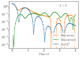
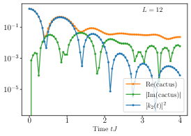
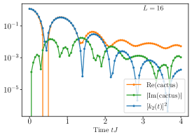
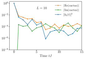
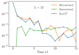
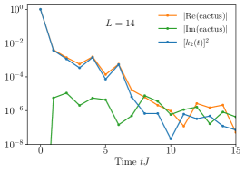
Figure S4: Factorization of the cactus diagram in the time domain. (Top row) The Ising model with system size $L=8,12,16$ and the collective observable. (Bottom row) Circuit with $L=10,12,14$ and the collective observable.

2 Factorization of non-crossing contribution in the time-domain

The general ETH predicts the factorization of the non-crossing contribution in time [c.f. Eq. (3) of the main text] as well as in the frequency domain. In the main text, we have studied the factorization at equal times and as a function of frequency in Fig. 2 of the main text. Here we discuss the factorization in the time domain. We consider the cactus contribution appearing in the OTOC of Eq. (17) of the main text, namely

$$\text{cactus}(t)=\text{cactus}(t,t)=\frac{1}{D}\sum_{i\neq j\neq m}e^{\mathrm{i}\omega_{ij}t+i\omega_{im}t}{|A_{ij}|^{2}|A_{im}|^{2}}$$ (S28)

with $\text{cactus}(t_{1},t_{2})$ is defined in Eq. (15). The factorization in Eq. (3) of the main text implies that in the large $L$ limit one shall have

$$\text{cactus}(t)\simeq[k_{2}(t)]^{2}+\mathcal{O}(1/L)\ .$$ (S29)

This factorization is checked numerically and the data are reported in Fig. S4 for the Hamiltonian case (top row) and the circuit (bottom row). For finite times, $\text{cactus}(t)$ develops an imaginary part, that oscillates around $t=0$ (in the figure we plot the absolute value) and it is suppressed as the system size increases. Furthermore, the agreement between $\text{Re (cactus}(t))$ and $[k_{2}(t)]^{2}$ holds up to a time scale which diverges in the limit $L\to\infty$.

3 Results for other operators

In this section, we discuss the numerical results for other operators, focusing first on local operators and secondly on other spin operators for the Ising model.

3.1 Local operators

We consider

$$\hat{A}=\hat{\sigma}^{y}_{L/2}\quad\text{Ising model}$$ (S30)

$$\hat{A}=\hat{\sigma}_{L/2}^{z}\quad\text{Circuit}\ .$$ (S31)

]

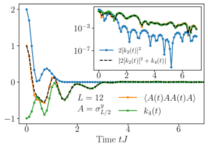
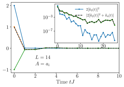
Figure S5: Multi-time correlation functions and ETH free-cumulants in chaotic systems. The full dynamics of $\langle A(t)AA(t)A\rangle$ (orange) is contrasted with the Gaussian contribution $2[k_{2}(t)]^{2}$ (blue), the free cumulant $k_{4}(t)$ (green) and the sum of the two (dashed), cf. Eq. (4) in the main text. In the inset, we plot the absolute value of the previous quantities. (Left) Ising model with $L=12$ and $\hat{A}=\sigma^{y}_{L/2}$. (b) Floquet circuit with $L=14$.

In Fig. S5 we show the dynamical moment-free cumulant decomposition for the OTOC [cf. Eq. (17)] for local operators. Now we have $\hat{A}^{2}=\hat{A}^{4}=1$, hence one has also $\langle A(0)AA(0)A\rangle=k_{2}(0)=1$. Since $\langle A^{4}\rangle=2[k_{2}(0)]^{2}+k_{4}(0)$, this means that the fourth free cumulant starts from a negative value: $k_{4}(0)=-1$. As for the collective operator, also here $k_{2}(t)$ approaches zero after a short time-scale, while the characteristic OTOC dynamics is given by $k_{4}(t)$. This is emphasized by the log plot of the inset, which shows that the fourth cumulant (green line) reproduces the full OTOC result up to very large times.

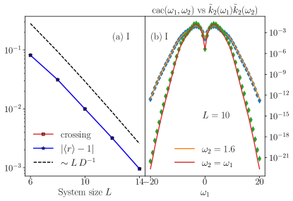
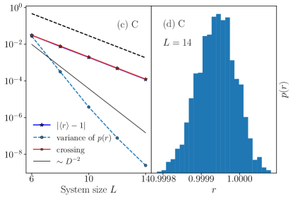
Figure S6: High-order ETH conditions (2-3) of the main text as a function of the system size $L$ in the Ising model (a-b) and the Floquet circuit (c-d) for local operators. (a) We denote with “crossing” Eq.(2), while $r$ corresponds to Eq.(14) of the main text, plotted as a function of the system size $L$. (b) Ising model factorization for $\hat{A}=\sigma^{y}_{L/2}$: the non-crossing contribution (full line) in Eq.(3 )of the main text is compared with the factorized result (diamonds) in the frequency domain, along two directions $\omega_{2}=1.6$ and $\omega_{2}=\omega_{1}$ for $L=16$. (d) Distribution of the ratio $r$ in the circuit for $L=14$. The variance of this distribution $p(r)$ as a function of $L$ is plotted in panel (c).

In Fig. S6, we look at the exponential suppression of crossing partitions [cf. Eq. (2) of the main text] and at the factorization of non-crossing parts [cf. Eq. (3) of the main text] for the Ising model (left) and for the circuit (right). We show the exponential suppression of the crossing partitions and the distance from one of the equal-times ratio $|\langle r\rangle-1|$ in Eq. (14). In the case of local unitary observables, i.e. $\hat{A}^{2}=1$, these two shall coincide. Let us perform the simple calculation

$$\text{cactus}(0,0) =\frac{1}{D}\sum_{i\neq j\neq k}|A_{ij}|^{2}|A_{ik}|^{2}\pm\frac{1}{D}\sum_{i\neq j}|A_{ij}|^{4}$$ (S32)

$$=\frac{1}{D}\sum_{i\neq j\,i\neq k}|A_{ij}|^{2}|A_{ik}|^{2}-\text{crossing}$$ (S33)

$$=\frac{1}{D}\sum_{i}\langle i|\hat{A}\sum_{k}|k\rangle\langle k|\hat{A}|i\rangle\,\langle i|\hat{A}\sum_{j}|j\rangle\langle j|\hat{A}|i\rangle-\text{crossing}$$ (S34)

$$=\frac{1}{D}\sum_{i}\langle i|\hat{A}^{2}|i\rangle\,\langle i|\hat{A}^{2}|i\rangle-\text{crossing }$$ (S35)

$$=\frac{1}{D}\sum_{i}|\langle i|i\rangle|^{2}-\text{crossing }=1-\text{crossing}\ ,$$ (S36)

where in the first line with $\pm$ indicates that we add and subtract the same quantity $\text{crossing}=\frac{1}{D}\sum_{i\neq j}|A_{ij}|^{4}$ (defined in Eq. (2) of the main text) and from Eq. (S33) to Eq. (S34) we have neglected the condition $i\neq j$ and $i\neq k$ since we deal with observables such that $A_{ii}=0$. Thus, since we have also $k_{2}(0)=1$ one immediately finds that

$$|\langle r\rangle-1|=|\frac{\text{cactus}(0,0)}{k_{2}(0)}-1|=\text{crossing}.$$ (S37)

In Fig. S6cd, we also consider the factorization as a function of frequency, i.e. $\text{cac}(\omega_{1},\omega_{2})\simeq\tilde{k}_{2}(\omega_{1})\tilde{k}_{2}(\omega_{2})$. For the Ising model, we report the data along two directions $\omega_{2}=\omega_{1}$ and $\omega_{2}=1.6$, which show good agreement. The differences that arise at large frequencies are due to the entropic corrections $\propto e^{-\frac{\partial^{2}S(E)}{\partial E^{2}}\Big{|}_{E=0}\omega^{2}/8}$. These are neglected in the standard ETH calculations (e.g. the ones leading to Eq. (3) in the main text) because they vanish in the thermodynamic limit for finite frequencies. They are however visible for finite $L$ at large $\omega$. In Fig. S6d we plot the histogram over all frequencies of $r(\omega_{1},\omega_{2})$, defined in Eq. (16) of the main text. In this case, the distribution has no feature at $\omega_{1}=\omega_{2}$ and its variance decreases faster than $D^{-2}$.

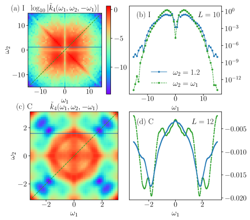
Figure S7: Frequency dependence of the fourth free cumulant $\tilde{k}_{4}(\omega_{1},\omega_{2},-\omega_{1})$ for local operators: for the Ising model, with $L=10$ $A=\sigma^{y}_{L/2}$ and smoothing with $\tau=5$ (a,b) and the Floquet circuit with $L=12$ and smoothing with $\tau=10$ (c,d). On the right (b,d), the frequency dependence is plotted along two directions $\omega_{1}=\omega_{2}$ (green) and $\omega_{2}=1.6$ (blue).

In Fig. S7 we show the data for the frequency-resolved fourth cumulant [cf. Eq. (18) of the main text] for the local observable. As for the global observable, the main difference between the Hamiltonian and the Circuit model is given by the fast decay at large frequencies of the former. We remark that in this case the $\tilde{k}_{4}(\vec{\omega}_{1},\omega_{2},-\omega_{1})$ is negative, in agreement with the fact that $k_{4}(t=0,t=0,t=0)=-1$ for local observables.

3.2 Other magnetization operators per the Ising model

Up to now we have only considered the magnetization along $y$ for the Ising model, which has the property $A_{nn}=0$. The validity of general ETH holds however for a much larger class of operators, as shown in Fig.S8, where we consider $\hat{S}^{z}/\sqrt{L}$ (Row 1) $\hat{S}^{x}/\sqrt{L}$ (Row 2), $\hat{A}=\hat{\sigma}_{1}^{z}\hat{\sigma}_{2}^{z}$ (Row 3), $\hat{A}=\hat{\sigma}_{L/2}^{z}$ (Row 4) and$\hat{A}=\hat{\sigma}_{L/2}^{x}$ in (Row 5). For the numerics we manually set to zero the diagonal matrix elements $A_{nn}$. This does not change the results, since the expectation value at infinite temperature vanishes, i.e. $\langle A\rangle=0$.

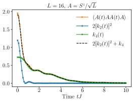
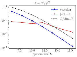
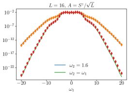
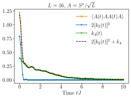
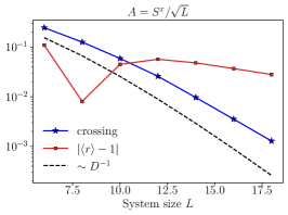
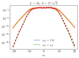
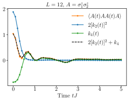
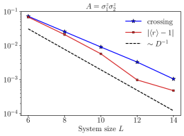
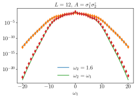
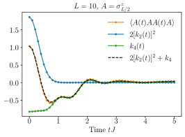
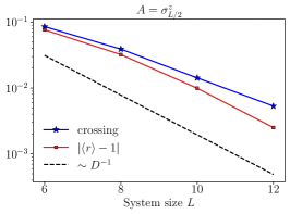
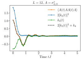
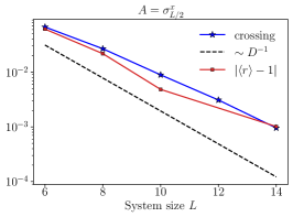
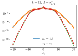
Figure S8: General ETH by free cumulants for different observables. Column 1: dynamics of the full OTOC compared with the free-cumulant decomposition, Column 2: higher-order ETH conditions as a function of the system size $L$ and Column 3: factorization of the non-crossing partition in the frequency domain. Row 1: $\hat{S}^{z}/\sqrt{L}$, Row 2: $\hat{S}^{x}/\sqrt{L}$, Row 3: $\hat{A}=\hat{\sigma}_{1}^{z}\hat{\sigma}_{2}^{z}$, Row 4: $\hat{A}=\hat{\sigma}_{L/2}^{z}$ and Row 5: $\hat{A}=\hat{\sigma}_{L/2}^{x}$. For the collective operators (rows 1-2) the calculation is restricted to the sector with $k=0$ and positive inversion, while for the local operators (rows 3-5) we consider the full Hilbert space, for this reason the calculation is restricted to smaller $L$.

4 Details on the Circuit model

For completeness, we report the unitary two-qubit gates used for numerical simulations in the Circuit model here. The gates are given by

$$U_{1}=\left(\begin{smallmatrix}0.67931743-\mathrm{i}0.0721112&0.51877751-\mathrm{i}0.04466678&0.25741725+\mathrm{i}0.08032817&-0.36793521-\mathrm{i}0.23261557\\ 0.3619221-\mathrm{i}0.46028992&-0.56476001+\mathrm{i}0.43994397&-0.09219379+\mathrm{i}0.36114353&-0.07557832-\mathrm{i}0.00214075\\ 0.13342533+\mathrm{i}0.37674694&-0.30800024+\mathrm{i}0.1579134j&0.62386475-\mathrm{i}0.20799404&-0.20374812+\mathrm{i}0.49646409\\ -0.13483809-\mathrm{i}0.11203347&-0.30258211+\mathrm{i}0.07080587&0.25709566-\mathrm{i}0.53832377&-0.15624451-\mathrm{i}0.70170847\end{smallmatrix}\right)$$ (S38)

and

$$U_{2}=\left(\begin{smallmatrix}-0.32936937+\mathrm{i}0.0575935&-0.32742441+\mathrm{i}0.30978811&-0.41818243+\mathrm{i}0.42081727&-0.14116509-\mathrm{i}0.55958207\\ -0.53553904-\mathrm{i}0.54762144&0.13993909-\mathrm{i}0.01096924&0.5221732+\mathrm{i}0.23437906&0.23558662-\mathrm{i}0.10249863\\ -0.09194887+\mathrm{i}0.40213391&-0.35024609+\mathrm{i}0.37068525&0.14797073+\mathrm{i}0.19071808&0.60159551+\mathrm{i}0.38674017\\ 0.02435271-\mathrm{i}0.36159117&-0.33621261+\mathrm{i}0.63561192&0.11961071-\mathrm{i}0.49785786&-0.2804114+\mathrm{i}0.10400783\end{smallmatrix}\right).$$ (S39)

References

Gallavotti [1999]G. Gallavotti, Statistical
mechanics: A short treatise (Springer Science &
Business Media, 1999).
Hruza and Bernard [2022]L. Hruza and D. Bernard, arXiv
preprint arXiv:2204.11680 (2022).
[57]See the Supplemental Material for additional
analysis and background calculations on 1. frequency-dependent free cumulants
in rotationally invariant random matrices, 2. numerical results on the
factorization of the non-crossing contributions in the time domain and 3. the
numerical estimation of ETH in the case of local operators.
Note [2]This is ensured by a sort of self-averaging of Eq. (S22\@@italiccorr) which is valid at the leading
order in , thus the fluctuations which would contribute to the cross term
in the average with the deltas are subleading.
——————————