Robust and Practical Solution of Laplacian Equations
by Approximate Elimination

Abstract

We introduce a new algorithm and software for solving linear equations in symmetric diagonally dominant matrices with non-positive off-diagonal entries (SDDM matrices), including Laplacian matrices. We use preconditioned conjugate gradient to solve the system of linear equations. Our preconditioner is a variant of the Approximate Cholesky factorization of Kyng and Sachdeva (FOCS 2016). Our factorization approach is simple: we eliminate matrix rows/columns one at a time, and update the remaining entries of the matrix by sampling entries to approximate the outcome of complete Cholesky factorization. Unlike earlier approaches, our sampled entries always maintain a connected graph on the neighbors of the eliminated variable. Our algorithm comes with a tuning parameter that upper bounds the number of samples made per original entry.

We implement our solver algorithm in Julia, and experimentally evaluate its performance when using 1 or 2 samples for each original entry: We refer to these variants as AC and AC2 respectively. We investigate the performance of these implementations and compare their single-threaded performance to that of current state-of-the-art solvers including Combinatorial Multigrid (CMG), BoomerAMG-preconditioned Krylov solvers from HyPre and PETSc, Lean Algebraic Multigrid (LAMG), and MATLAB’s preconditioned conjugate gradient with Incomplete Cholesky Factorization (ICC). Our experiments suggest that AC2 and AC attain a level of robustness and reliability not seen before in solvers for SDDM linear equations, while retaining good performance across all instances.

Many large-scale evaluations of SDDM linear equation solvers have focused on solving problems on discretized 3D grids. We conduct evaluations across a much broader class of problems, including all large SDDM matrices from the SuiteSparse collection, as well as a broad array of programmatically generated instances. Our tests range up to 200 million non-zeros per system of linear equations. Our experiments show that AC and AC2 obtain good practical performance across many different types of SDDM-matrices, and significantly greater reliability than existing solvers. AC2 is the only solver that succeeds across all our tests, and it uses less than $7.2\mu s$ time per non-zero across to converge to $10^{-8}$ relative residual error across all our experiments. AC is typically 1.5-2 times faster, but fails on one family of problems engineered to attack this algorithm. In our experiments using general sparse non-zero patterns, CMG, HyPre, PETSc, and ICC all fail on some instances from a majority of the families tested. Across these families, the median running time across different instances of AC2 and AC is comparable to or faster than other solvers.

We also test the performance of our solvers on a wide array of Poisson problems on 3D grids, including grids with uniform, high-contrast, or anisotropic coefficients, and grids from the SPE Benchmark. Here, the CMG and HyPre solvers perform best, but AC and AC2 achieve worst case and median running times within a factor 4.1 and 6.2 of these respectively.

Our code is public, and we detail precisely the set of tests we run and provide a tutorial on how to replicate the tests. We hope that others will adopt this suite of tests as a benchmark, which we refer to as SDDM2023. Our solver code is available at:

https://github.com/danspielman/Laplacians.jl/

Our benchmarking data and tutorial is available at:

https://rjkyng.github.io/SDDM2023/

1 Introduction

Linear equations in symmetric diagonally dominant matrices with non-positive off-diagonal matrices (SDDM) matrices appear in many applications, including solvers for discretized scalar elliptic partial differential equations [vM77, Ker78, CB01, BHV08, SBB⁺12], many problems in computer vision and computer graphics [KMT11], and in machine learning [ZGL03]. They are essentially equivalent to the Laplacian matrices of graphs.

In this paper, we introduce a new algorithm for solving SDDM linear equations, as well as an single-threaded implementation of the algorithm and several variations in Julia. We assemble a large suite of SDDM matrices on which to to test solvers, and use these to evaluate the performance of our implementation and to compare it with other popular solvers for SDDM linear equations. We include important test cases from finite-difference method approaches to solving scalar ellipic partial differential equations, all SDDM matrices from the SuiteSparse collection, other classic benchmark data, and several programmatically generated difficult instances, including problems coming from running Interior Point Methods for linear programming. We hope this collection of matrices will be adopted as a benchmark in future work. One can use a reduction of Gremban [Gre96] to convert the problem of solving an $n\times n$ SDD linear equation into one of solving a $2n+1\times 2n+1$ Laplacian linear equation, but in this work we do not test the performance of our algorithm on instances coming from general SDD matrices.

Current popular implementations of SDDM solvers [HY02, BGH⁺19, LB12] rely on variants of multigrid methods [Bra77, Bra02]. There has been tremendous theoretical success in developing SDDM linear equation solvers with running times asymptotically nearly-linear in the number of non-zeros of the matrix starting with the work of Spielman and Teng  [ST04, KMP10, KMP11, KOSZ13, PS14, KLP⁺16, KS16, JS21, HJPW23], but so far, these algorithms have not lead directly to practical solver implementations. This line of work on asymptotically fast solvers builds on support theory, an approach to preconditioning Laplacian linear equations that expands on a breakthrough of Vaidya [Vai90, Gre96, BH03, BCHT04, BGH⁺06a]. Ideas from support theory have also had significant impact on the Combinatorial Multigrid Solver by Koutis, Miller, and Tolliver [KMT11], which combined these ideas with a multi-grid approach.

1.1 Related Work

Code and experiments.

Incomplete Cholesky factorizations were introduced by Meijerink and van der Vorst [Mv77] to accelerate the solution of systems of linear equations in symmetric M-matrices. These are obtained by omitting most entries that appear during Cholesky factorization, and the factorization they produce can be shown to crudely approximate the original matrix. Meijerink and van der Vorst suggested using these factorizations as a preconditioners for the Conjugate Gradient. When they were introduced, they provided the fastest solutions to the discrete approximations of two-dimensional elliptic PDEs. A popular implementation of this method is MATLAB’s ichol. Two key differences between these factorizations and our new Approximate Choleksy factorizations are that the Approximate Cholesky factorizations increase the magnitudes of the entries they keep and that they select entries to keep at random.

The Multigrid algorithm [BD79] provided a significant improvement in the solution of systems of equations arising from discrete approximations of elliptic PDEs, and its generalizations provide the fastest solvers for many families of linear equations. Algebraic Multigrid (AMG) builds upon the principles of Multigrid methods but has a wider range of applications as it does not require the problem to have a simple underlying geometry, making it applicable to general symmetric M-matrices [RS87], a family that includes SDDM matrices. Brandt designed an AMG solver applicable to Dirac equations [Bra00]. For linear equations in graph Laplacians, Livne and Brandt presented a variant of AMG solver, called the Lean Algebraic Multigrid (LAMG), and provided a MATLAB implementation [LB12]. Another multi-grid variant specialized for graph Laplacians was developed by Napov and Notay [NN17].

BoomerAMG, a parallel AMG implementation, was introduced in [HY02], and can be accessed via the popular software library HyPre [FY02]. The Portable, Extensible Toolkit for Scientific Computation (PETSc) provides another interface for accessing the HyPre-BoomerAMG implementation and its own implementations of conjugate gradients [BAA⁺19]. Combinatorial Multigrid (i.e. CMG) [KMT11] is a solver that combines ideas from support theory [Vai90, BH03] with ideas from (Algebraic) Multigrid methods. The MATLAB implementation of CMG was applied to problems arising in computer vision and image processing in [KMT11]. [LHL⁺19] presented another implementation of CMG in C using PETSc, however, to the best of our knowledge, this implementation is not publicly available. As part of the Trilinos software package, MueLu [BGH⁺19] provides a multigrid algorithm designed for solving sparse linear systems of equations arising from PDE discretizations using massively parallel computing environments.

In [CT03], Chen and Toledo evaluated an SDD solver based on Vaidya’s ideas on tree-based preconditioning combined with PCG. They compared the solver with PCG preconditioned using Incomplete Cholesky factorization and that Vaidya’s approach was often much slower, but sometimes lead to convergence in cases where Incomplete Cholesky with PCG did not. In [DGM⁺16], Deweese et al. studied the performance of variants of the cycle toggling SDD solver from [KOSZ13]. This algorithm works in with a ‘dual space’ representation (sometimes known as the ‘flow space’). The paper focused on contrasting these implementations without a direct comparison to other solvers. In [BDG16], Boman, Deweese, and Gilbert evaluated a cycle toggling algorithm in ‘primal space’ (‘voltage space’) known as Primal Randomized Kaczmarz (PRK). They compared this with an implementation of the [KOSZ13] solver and with a PCG implementation using Jacobi diagonal scaling. The authors find that their results “do not at present support the practical utility of” cycle toggling solvers in primal or dual space. Hoske et al. reached similar conclusions in another experimental evaluation of an implementation of the [KOSZ13] cycle toggling solver [HLMW16].

A recent paper by Chen, Liang, and Biros has provided another implementation of our sampling procedure  [CLB21] though only the single sample-version (corresponding to our AC implementation). Unlike our implementation, the authors used the standard Cholesky lower-triangular format for the output, whereas our implementation uses a row-operation representation of the output. Chen et al. use a METIS-based elimination ordering while ours is adaptive. Chen et al. have developed a parallel version of the algorithm and code using nested dissection ordering. Their implementation, known as RCHOL, is available at https://github.com/ut-padas/rchol via C++/MATLAB/Python interfaces. Chen, Liang, and Biros  [CLB21] experimental evaluation focused on comparing RCHOL with three other solvers: (1) the MATLAB’S preconditioned conjugate gradient combined with the ichol implementation of Incomplete Cholesky factorization, (2) Ruge–Stuben AMG (RS-AMG from pyamg), (3) the smoothed aggregation AMG (SA-AMG also from pyamg), and (4) Combinatorial Multigrid [KMT11]. Their experiments were based on three matrices arising from 3D grid Poisson problems (with uniform, variable, and anisotropic coefficients) and four matrices from the SuiteSparse matrix collection: one SDD, one SDDM and two which are neither. They found that RCHOL outforms ichol, and found each of the four solvers RCHOL, CMG, RS-AMG, and SA-AMG performs best on some of the tested problems.

Theory.

There are some theories of convergence for (Algebraic and Geometric) Multigrid methods [BH83, Yse93] and preconditioned iterative methods using Incomplete Cholesky factorization [Mv77, Gus78, Bea94, Not90, Not92, BGH⁺06b], but these do not establish fast rates for general SDDM matrices.

Spielman and Teng [ST04] built on the work of Vaidya [Vai90] to develop the first provably correct nearly-linear time algorithm for solving SDD linear equations [ST04]. Koutis, Miller and Peng substantially simplified the algorithm of Spielman and Teng and greatly reduced its running time [KMP10, KMP11]. Building on this line of work, [CKP⁺14] reduced the running time below that of comparison sorting the input, and recently [JS21] reduced the running time to linear in the number of matrix non-zeros, up to poly-loglog factors and a $\log(1/\epsilon)$ dependence on the error, $\epsilon$. The solver of Kelner et al. introduced a dual-solution based approach, resulting a simple algorithm, once a low-stretch spanning tree for the matrix has been computed. Another line of work introduced a parallel algorithm [PS14] and removed the reliance on combinatorial sparsification [KLP⁺16]. Finally, [KS16] introduced and analyzed a very simple algorithm that is the inspiration for the algorithm in the present paper.

2 Results and Conclusion

We introduce a variant of the approximate Cholesky factorization algorithm developed in [KS16] that greatly improves its practical performance while retaining its simplicitly. Our algorithm solves linear equations in SDDM matrices, including Laplacian matrices. We conduct extensive experiments, testing the performance of two variants of our algorithm across a wide range of SDDM matrices and comparing our solver with a suite of state-of-the-art solvers. Our experiments measure the single-threaded performance of these solvers. The experiments cover a broad range of equations in SDDM matrices, including Laplacian matrices.

2.1 Algorithms and Implementation

Our algorithm solves an SDDM linear equation by reducing it to a Laplacian linear equation, computing an approximate Cholesky factorization of that Laplacian matrix, and using it as a preconditioner for the Laplacian inside the Conjugate Gradient. The basic version of our algorithm eliminates rows (and the corresponding column) of a Laplacian matrix one at a time. For each off-diagonal entry in the eliminated row, a new entry is sampled and inserted into the remaining matrix, while guaranteeing two important properties: first, the expected value of the output samples agree exactly with the output of Cholesky factorization, and second, the sampled non-zeros preserve the connectivity structure of the graph. Concretely, if the off-diagonal entries are viewed as edges in a graph with vertices corresponding to the rows/columns of the matrix, then the algorithm can be seen as eliminating the edges incident to a vertex and replacing them with a tree on the neighbors of the vertex. In our implementations, we eliminate vertices with whose degree is approximately minimum at the time they are eliminated. As the edges introduced during elimination are random, the resulting elimination order appears unrelated to the approximate minimum degree ordering [ADD96]. In our approximate factorization approaches, the order of elimination of edges also changes the algorithm, and our implementation eliminates edges in the order of lowest to heighest weight.

We refer to our implementation of the basic version of our algorithm as Approximate Cholesky (AC). Experimentally, we find that AC performs well on a large range of SDDM matrices. However it performs poorly on matrices that were specially designed by Sushant Sachdeva to make it fail. We call these Sachdeva stars. To address the problem caused by these examples, we develop a more robust, but slightly slower, version of the algorithm: this version divides each matrix entry into $k$ separate “multi-entries” (analogous to multi-edges in a graph). After this, we run the original algorithm on this structure – but now the output of each sampled elimination has the non-zero structure of a union of trees with at most as many multi-entries as the eliminated row/column. At $k=2$, i.e. with just two multi-entries per original entry, this robust version of the algorithm performs well across all our tests. We refer to this version of our algorithm as AC2. While our algorithm has not been rigorously analyzed, the design of the sampling procedure is motivated in part by [KS16], as well as theoretical work which suggests graphs may be well-approximated by a tree plus a few additional edges: tree-based ultra-sparse sampling can yield convergent iterative methods for solving Laplacians [ST04], even when the sampling is too sparse to yield concentration of measure w.r.t. spectral norms [CKP⁺14]; and in bounded degree graphs, a union of two random spanning trees forms a good cut sparsifier [GRV09], while a few random spanning trees form a good spectral sparsifier [KS18, KKS22].

The output of our algorithm can be represented in two different ways: either as a standard lower-triangular Cholesky factorization or as a product of row operation matrices. Regarded as linear operators, the two are identical (i.e. when using the same source of randomness they will output identical linear operators), but it is unclear which performs better in practice, and which version has better numerical stability. Our implementation uses the product of row operations form.

Our solvers are implemented in Julia and are available at: . https://github.com/danspielman/Laplacians.jl/

2.2 Experimental Evaluation and Comparison

Solvers.

We run a broad suite of experiments, measuring the single-threaded performance of our AC and AC2 solvers and comparing them with the following suite of popular SDDM linear equation solvers:

• Combinatorial Multigrid (CMG),

• HyPre’s Krylov Solver with BoomerAMG preconditioning (HyPre),

• PETSc’s Krylov Solver with BoomerAMG preconditioning (PETSc),

• MATLAB preconditioned conjugate gradient using the ichol implementation of Incomplete Cholesky factorization (ICC),

• Lean Algebraic Multigrid (LAMG).

Of the third-party solvers we test, i.e. CMG, HyPre, PETSc, ICC, and LAMG, the latter three seem to be dominated in performance by CMG or HyPre, with few exceptions. Consequently, our discussion will focus on comparing AC and AC2 with CMG and HyPre.

Summary of experimental results.

We test three main categories of SDDM matrices.

1. All large SDDM matrices in SuiteSparse.

2. Programmatically generated matrices:

   1. “Chimeras”: a broad class of matrices that we generate programmatically to test solvers on a wide array of graph geometries.

   2. “Sachdeva stars”: A special family of matrices designed to challenge our algorithm.

   3. “Flow Interior Point Method Matrices”: We create variants of our “Chimeras” with different entries by running an Interior Point Method for a maximum flow problem on these graphs. This creates a sequence of linear equations in SDDM matrices with the same non-zero structure as the input graph, but with a challenging weight pattern. We also create sequences of SDDM matrices by running a maximum flow interior point method on Spielman graphs, a family of graphs that are thought to be particularly challenging for interior point methods.

3. Discretizations of partial differential equations on 3D grids:

   1. Matrices based on fluid simulations from a Society of Petroleum Engineering (SPE) benchmark.

   2. Poisson problems on 3D grids with uniform, high-contrast coefficients, or anisotropic coefficients.

The matrices we use have up to 200 million non-zeros.

AC2 is able to convergence in a reasonable time on every single test, while AC is typically faster but fails to converge on large Sachdeva stars. On general graphs, our solvers achieve a worst-case running time of about 7.2 $\mu s$ per non-zero entry, while on grid graphs we get a worst-case running time of about 3.6 $\mu s$ per non-zero. This should be contrasted with all other solvers we test, which fail entirely fail to converge both on some matrices from SuiteSparse and some Chimeras, but achieve a worst case running time on grid graphs of about 0.67 $\mu s$ per non-zero (CMG) and $0.77$ $\mu s$ per non-zero (HyPre). Our experiments show that AC and AC2 obtain good practical performance across many different types of SDDM-matrices, and significantly greater reliability than existing solvers.

Our test results are summarized in Table 1.

Instance family	AC	AC2	CMG	HyPre	PETSc	ICC
	$t_{\text{total}}/\operatorname{nnz}$		$t_{\text{total}}/\operatorname{nnz}$
	$(\mu s)$	$(\mu s)$	$(\mu s)$	$(\mu s)$	$(\mu s)$	$(\mu s)$
SuiteSparse Matrix Collection	$0.994$	$1.4$	Inf	Inf	$27.1$	$153$
Unweighted Chimeras	$3.95$	$7.19$	Inf	Inf	Inf	Inf
Weighted Chimeras	$4.39$	$4.79$	Inf	Inf	N/A	Inf
Unweighted SDDM Chimeras	$3.4$	$5.44$	Inf	Inf	Inf	Inf
Weighted SDDM Chimeras	$4.34$	$4.36$	Inf	Inf	N/A	Inf
Maximum flow IPMs	$1.2$	$2.39$	$1.9$**	$5.04$*	N/A	Inf
Sachdeva stars	$4.76$**	$1.04$	$0.868$	$3.52$**	$7.22$**	Inf
SPE benchmark	$1.62$	$1.91$	$0.511$	$0.648$	$2.58$	$4.29$
Uniform coefficient Poisson grid	$1.46$	$2.49$	$0.624$	$0.587$	$2.62$	$2.22$
High contrast coefficient Poisson grid	$2.33$	$3.57$	$0.572$	$0.752$	$3.85$	$4.76$
Anisotropic coef. Poisson grid, variable discretization	$1.48$	$2.5$	$0.659$	$0.614$	$2.6$	$1.92$
Anisotropic coef. Poisson grid, variable weight	$1.67$	$2.5$	$0.674$	$0.772$	$4.92$	$2.44$

• relative residual error exceeded tolerance $10^{-8}$ by a factor $(1,10^{4}]$.

• relative residual error exceeded tolerance $10^{-8}$ by a factor $(10^{4},10^{8})$.

• Inf: Solver crashed or returned a solution with relative residual error 1 (error of the trivial all-zero solution).

• N/A: Experiment omitted as the solver crashed too often with (only occurred for PETSc).

Table 1: Summary of worst case total solve time per non-zero matrix entry across all experiments.

Experiments on SuiteSparse SDDM matrices.

We test the solvers on every SDDM matrix currently hosted on the SuiteSparse Matrix Collection, previously known as the University of Florida Sparse Matrix Collection [DH11], after excluding very small matrices (with less than 1000 non-zero entries) to limit the impact of start-up overhead. AC2 and AC converge on all these problems in time at most 1.4 $\mu s$ per non-zero. Meanwhile HyPre and CMG fail on some instances, and PETSc and ICC respectively take 27.1 $\mu s$ and 153 $\mu s$ per non-zero in the worst case. AC2 and AC are also faster than CMG, PETSc, and ICC in median times, but slower than HyPre on median times. See Table 5.3.1 for these results.

Experiments on programmatically generated SDDM matrices.

We created a generator for weighted Laplacian matrices that we call Laplacian Chimeras because they combine matrices of many types. The results of these experiments on these are shown in Tables 5.3.2 and 5.3.2. We test the suite of solvers on these, as well as a set of strictly diagonally dominant matrices derived from the Laplacian Chimeras. Results are shown in Tables 5.3.2 and 5.3.2. Across the Laplacian and SDDM Chimeras we test, both CMG and HyPre fail on some instances. On these Chimeras, the median running time of AC and AC2 is lower than for CMG and HyPre. Thus both the worst case performance and the typical performance of AC and AC2 beats that of CMG and HyPre on this class of problems.

We test our solvers on an additional generated family of graphs, which we refer to as Sachdeva stars, designed specifically to challenge our family of algorithms. On Sachdeva stars, AC2 converges and AC fails to converge. Results for Sachdeva stars are shown in Table 1.

In addition to our tests on unweighted and randomly weighted Chimeras, we run experiments based on using our Laplacian matrix linear equation solvers inside an Interior Point Method (IPM) that solves an Undirected Maximum Flow Problem to high accuracy. Laplacian linear equations arise in IPM algorithms for single-commodity flow problems because the algorithms proceed by taking Newton steps that minimize a sequence of barrier function problems, and each Newton step corresponds to a Laplacian linear equation. Laplacian linear equations arising from IPMs tend to have very large ranges of weights, which leads to ill-conditioned problems, and currently, to the best of our knowledge, no Laplacian solver has been reliable enough to use in IPMs. First, we consider Maximum Flow Problems on unweigted Chimera graphs. We use a short-step IPM and solve the problems to high accuracy, see Table 5.3.4 for results. Second, we consider a special family of graphs, known as Spielman graphs, which are conjectured to be a particularly hard instance for short-step IPMs. The results of this experiment are shown in Table 5.3.4. Our IPM is conservative and uses far too many Newton steps to be practical, but the experiments demonstrate that, at least for short-step IPMs, both AC and AC2 work reliably across many different instances. We believe this suggests that AC and AC2 may be good candidates for further research into developing Interior Point Methods for single-commodity flow problems using fast linear equation solvers. In contrast, all the other tested solvers fail on some IPM instances – which is unsurprising as the solvers even fail on unweighted Chimera instances, and the IPM should create similar instances but with more extreme weights.

Experiments on 3D grid discretizations.

We find that the HyPre and CMG solvers are the fastest on grid problems, up to 4.1 times faster than AC and 6.3 times faster than AC2, see Tables 4, 5, 6, 7, and 3. Our experiments on grids include both SDDM matrices generated from fluid flow problems using data from the Tenth SPE Comparative Solution Project [CB01], from the Society of Petroleum Engineering (SPE), as well as Poisson 3D grids with uniform coefficients, high contrast coefficients, or anisotropic coefficients. These experiments suggest that our current implementation of AC and AC2 is slower than state-of-the-art solvers on 3D grid problems – but the gap might be addressable by further optimization of our code.

Performance variability experiments.

We run tests to demonstrate the low variability in the performance of AC2 and AC, showing that their running times are reliable and consistent across many runs, see Table 5.4. We also run some experiments to shed light on why the more reliable AC2 algorithm outperforms AC in some settings. In particular, we show that AC2 builds a preconditioner with much smaller relative condition number on difficult instances, see Table 5.5.

Running time scaling with problem size.

In Section 5.7, we show plots that display the running time of our AC and AC2 solvers plotted against non-zero count, demonstrating that the observed scaling of running time in problem size is nearly-linear. Our plots for AC appear in Figures 3 and 4 and for AC2 in Figures 5 and 6.

2.3 Conclusion

Our experiments suggest that AC2 and AC attain a level of robustness and reliability not seen before in solvers for SDDM linear equations, while retaining good performance across all instances. For most problems, AC appears to be a good choice, while some very challenging instances require using AC2.

We hope that our benchmarking data will be used in future works to provide a rigorous basis for comparison of new SDD solvers. This benchmarking data and an accompanying tutorial are available at: https://rjkyng.github.io/SDDM2023/

Future work.

We plan to release a version of our code designed to handle symmetric diagonally dominant (SDD) matrices, which can have postitive off-diagonal entries, and symmetric block-diagonally dominant matrices (SBDD).

Open problems.

We hope that our results will motivate others to study ways to incorporate insights from our solvers into production level codes for solving SDDM systems. Developing a highly-optimized version of our algorithm, even for single-threaded systems, will be an important step in this discussion rection. Creating an efficient parallel implementation is even more important, and presents interesting questions about which parallelization approach is likely to be most successful. We believe a more in-depth study of the impact of elimination orderings is also warranted. For the particular case of 3D grid problems, [CLB21] studied the performance of many different elimination orders, however, it is not clear their observations how this translates beyond this case. They also developed a parallel implentation for 3D grid problems.

We believe the crucial feature of our algorithm is that it produces an unbiased approximate factorization while always maintaining connectivity in every elimination, and using slightly more samples than just a tree (in the case of AC2). However, many different elimination rules fullfill these criteria, and we suspect that rules with even better practical performance can be found.

We believe our solvers may finally be robust enough to use in Interior Point Methods, and we hope this will lead to further applied research on IPMs for single-commodity flow problems.

To further improve SDD solvers and to bring them into widespread practical use for applications such as IPMs, we believe more testing is required. Adding more benchmark data sets could serve as an important guide to which algorithms perform well in practice in these settings.

Organization of the paper

In Section 3, we introduce some standard facts about SDDM matrices, Laplacian matrices, and linear algebra relating to Cholesky factorization of these.

In Section 4.2, we introduce the pseudo-code for our approximate Cholesky factorization. We first describe a version which outputs an approximate factorization in standard lower triangular form. In Section 4.3, we show how to introduce multi-entry (a.k.a. multi-edge) splitting and merging into the approximate factorization algorithm. Combined with preconditioned conjugate gradient, this yields our AC2 implementation. In Section 4.4, we describe an alternative representation of the output factorization using row operations. Our AC implementation combines this row operation format with the preconditioned conjugate gradient to obtain a linear equation solver.

In Section 5, we describe our implementations and compare them to other solvers.

Acknowledgements

The authors want to thank Sushant Sachdeva, Richard Peng, Joel Tropp, George Biros, Houman Owhadi, and John Gilbert for many helpful conversation about practical solvers for SDDM linear equations. We thank Sushant Sachdeva for suggesting the Sachdeva Star to break the AC solver. We also thank Kaan Oktay for assistance with setting up PETSc and running experiments.

Contents

1. 1 Introduction
   1. 1.1 Related Work
2. 2 Results and Conclusion
   1. 2.1 Algorithms and Implementation
   2. 2.2 Experimental Evaluation and Comparison
   3. 2.3 Conclusion
3. 3 Preliminaries
4. 4 A Linear Equation Solver for Laplacian Matrices
   1. 4.1 Background: Approximate Cholesky Factorization of Laplacian Matrices
   2. 4.2 Edgewise Elimination and A New Clique Sampling Rule
   3. 4.3 A More Accurate Sampling Rule Using Multi-Edge Sampling
   4. 4.4 A Row-Operation Format for Cholesky Factorization Output
   5. 4.5 Our Full Algorithms
5. 5 Experimental Evaluation
   1. 5.1 Implementation
   2. 5.2 Solver Comparisons: Summary of Experiments
   3. 5.3 Solver Comparisons: Description of Experiments and Results
      1. 5.3.1 SuiteSparse Matrix Collection
      2. 5.3.2 “Chimera” Graph Laplacian and SDDM Problems.
      3. 5.3.3 Sachdeva Star Graph Laplacians.
      4. 5.3.4 Interior Point Method Matrices
      5. 5.3.5 SPE Benchmark
      6. 5.3.6 Poisson Problems on 3D Domains
   4. 5.4 Variation in the Performance of our Solvers
   5. 5.5 Comparison of Algorithm Variants: Splitting and Merging
   6. 5.6 Comparison of Algorithm Variants: Elimination Order
   7. 5.7 Running Time Scaling with Problem Size
6. A Linear Algebra and Cholesky Background
7. B Unbiased approximate Cholesky factorization
8. C Equivalence of the output representations

3 Preliminaries

In this section, we introduce several families of matrices for which we are able to construct fast linear system solvers.

Symmetric Diagonally Dominant (SDD) matrices.

A matrix $\bm{\mathit{M}}\in\mathbb{R}^{n\times n}$ is said to be Symmetric Diagonally Dominant (SDD), if it is symmetric and for each row $i$,

$$\bm{\mathit{M}}(i,i)\geq\sum_{j\neq i}\left|\bm{\mathit{M}}(i,j)\right|.$$ (1)

It can be shown that every SDD matrix is positive semi-definite.

Symmetric Diagonally Dominant (SDDM) matrices.

A matrix $\bm{\mathit{M}}\in\mathbb{R}^{n\times n}$ is said to be Symmetric Diagonally Dominant (SDDM) if it is SDD and has non-positive off-diagonal entries.

Graph Laplacians a.k.a. Laplacians.

We consider an undirected graph $G=(V,E)$, with positive edges weights $w:E\to\mathbb{R}_{+}$. Let $n=\left|V\right|$ be the number of vertices and , $m=\left|E\right|$ the number of edges, and $V=\left\{1,\ldots,n\right\}$. Let $\bm{\chi}_{i}$ denote the $i^{\textrm{th}}$ standard basis vector. Given an ordered pair of vertices $(u,v)$, we define the pair-vector $b_{u,v}\in\mathbb{R}^{n}$ as $\bm{\mathit{b}}_{u,v}=\bm{\chi}_{v}-\bm{\chi}_{u}.$ For a edge $e$ with endpoints $u$ and $v$ (arbitrarily ordered), we define $\bm{\mathit{b}}_{e}=\bm{\mathit{b}}_{u,v}.$ By assigning an arbitrary direction to each edge of $G$ we define the Laplacian of $G$ as $\bm{\mathit{L}}=\sum_{e\in E}w(e)\bm{\mathit{b}}_{e}\bm{\mathit{b}}_{e}^{\top}.$ Note that the Laplacian does not depend on the choice of direction for each edge. Given a single edge $e$, we refer to $w(e)\bm{\mathit{b}}_{e}\bm{\mathit{b}}_{e}^{\top}$ as the Laplacian of $e$. The Laplacian of a weighted, undirected graph is unique given the graph and vice versa, and we will treat these as interchangeable given this equivalence.

Laplacians and multi-graphs.

For some variants of our algorithms, we will need to work with multi-graphs. We can consider an undirected multi-graph $G=(V,E)$ with positive multi-edges weights $w:E\to\mathbb{R}_{+}$. Note that different multi-edges between the same vertices may have different weights. In this setting, we again let $n$ denote the number of vertices and we let $m=\left|E\right|$ denote the number of multi-edges. Similar to the case of graphs without multi-edges, we can assign arbitrary directions to multi-edges to define the Laplacian of a multi-edge $e$ as $w(e)\bm{\mathit{b}}_{e}\bm{\mathit{b}}_{e}^{\top}$ and define the Laplacian of $G$ as $\bm{\mathit{L}}=\sum_{e\in E}w(e)\bm{\mathit{b}}_{e}\bm{\mathit{b}}_{e}^{\top}.$ Note that different multi-graphs may have the same Laplacian. This occurs because the coefficient of the term $\bm{\mathit{b}}_{(u,v)}\bm{\mathit{b}}_{(u,v)}^{\top}$ only depends on the sum $\sum_{e\in E_{uv}}w(e)$ where $E_{uv}$ is the set of multi-edges between vertices $u$ and $v$. Thus, for example, we can take a multi-graph $G$ and produce another multi-graph $G^{\prime}$ with the same Laplacian by splitting each multi-edge $e$ of $G$ into $k$ copies with weight $w(e)/k$ each.

In Section 4.3, we introduce algorithms that use multi-graphs when computing an approximate Cholesky factorization of a Laplacian.

Fact 3.1.

If $G$ is connected, then the kernel of the corresponding Laplacian $\bm{\mathit{L}}$ is the span of the vector $\bm{1}.$

Upper and lower triangular matrices.

We say a square matrix $\bm{\mathit{{\mathcal{U}}}}$ is upper triangular if it has non-zero entries $\bm{\mathit{{\mathcal{U}}}}(i,j)\neq 0$ only for $i\leq j$ (i.e. above the diagonal). Similarly, we say a square matrix $\bm{\mathit{{\mathcal{L}}}}$ is lower triangular if it has non-zero entries $\bm{\mathit{{\mathcal{L}}}}(i,j)\neq 0$ only for $i\geq j$ (i.e. below the diagonal). Often, we will work with matrices that are not upper or lower triangular, but which for we know a permutation matrix $\bm{\mathit{P}}$ s.t. $\bm{\mathit{P}}\bm{\mathit{{\mathcal{U}}}}\bm{\mathit{P}}^{\top}$ is upper (respectively lower) triangular. For computational purposes, this is essentially equivalent to having a upper or lower triangular matrix, and we will refer to such matrices as upper (or lower) triangular. The algorithms we develop for factorization will always compute the necessary permutation.

4 A Linear Equation Solver for Laplacian Matrices

Our linear equation solvers are based on Preconditioned Conjugate Gradient (PCG), largely following [BBC⁺94]. Our approach to testing for stagnation is largely based on the MATLAB PCG implementation. We also refer the reader to the textbook by Golub and Van Loan [GVL13, Chapter 11] for additional background. We assume the reader is familiar with basics of PCG and preconditioners.

Our goal in this section is to describe our algorithm(s) for computing approximate Cholesky factorizations of Laplacian matries, which we then use as preconditioners inside the PCG. We use the overall algorithmic framework of [KS16], but we introduce a new approximate elimination rule that seems to perform much better in practice. In particular, it yields a good preconditioner with a much lower sampling rate than that of [KS16].

We reduce the problem of solving linear equations in SDDM matrices to that of solving linear equations in Laplacian matrices by using a technique introduced by Gremban [Gre96, Lemma 4.2]: An SDDM Matrix $M$ can be written in the form $D+L$ where $L$ is a Laplacian and $D$ is a non-negative diagonal matrix. Let $d$ be the vector of entries on the diagonal of $D$. Gremban constructs a Laplacian matrix $\widehat{L}$ that is identical to $L$ except that it has one extra vertex that is connected to vertex $i$ by an edge of weight $d[i]$. To solve the system $Mx=b$, we first solve $\widehat{L}y=\hat{b}$ where $\hat{b}$ is identical to $b$ except at the extra vertex, where its value is set to make the sum of the entries of $\hat{b}$ zero. The vector $x$ is then obtained by subtracting the value of $y$ at the extra vertex from the values of $y$ at the original vertices.

4.1 Background: Approximate Cholesky Factorization of Laplacian Matrices

In this section, we briefly review the how to compute a Cholesky factorization of a Laplacian matrix, using the additive formulation of [KS16]. We then briefly discuss how the elimination clique that arises from each row and column elimination can be sampled and how this yields a fast algorithm for approximate Cholesky decomposition [KS16]. This approximate Cholesky decomposition may then be used as a preconditioner in PCG to build a linear equation solver.

Producing a Cholesky factorization.

Cholesky factorization expresses a matrix in the form $\bm{\mathit{{\mathcal{L}}}}\bm{\mathit{{\mathcal{L}}}}^{T}$. A Cholesky factorization can be found for every symmetric positive definite matrix, and for every positive semidefinite matrix after a possible permutation of its rows and columns. One perspective on Cholesky factorization is that it proceeds by writing a symmetric positive semi-definite matrix as a sum of rank 1 matrices. We will outline this view here.

Let $\bm{\mathit{M}}$ be a symmetric positive semi-definite matrix. As a convenient notational convention, we define $\SS^{(0)}\stackrel{{\scriptstyle\mathrm{def}}}{{=}}\bm{\mathit{M}}$, the “0th” Schur complement. We then define

$$\bm{\mathit{l}}_{i} =\frac{1}{\sqrt{\SS^{(i-1)}(i,i)}}\SS^{(i-1)}(:,i)$$

$$\SS^{(i)} =\SS^{(i-1)}-\bm{\mathit{l}}_{i}\bm{\mathit{l}}_{i}^{\top},$$

unless $\SS^{(i-1)}(i,i)=0$, $\SS^{(i-1)}(:,i)=\bm{0}$, and $\SS^{(i-1)}(i,:)=\bm{0}$, in which case we define $\SS^{(i)}=\SS^{(i-1)}$. We do not define the Schur complement when the diagonal is zero but off-diagonals are not. By setting

$$\bm{\mathit{{\mathcal{L}}}}=\begin{pmatrix}\bm{\mathit{l}}_{1}&\bm{\mathit{l}}_{2}&\cdots&\bm{\mathit{l}}_{n}\end{pmatrix}$$

we get a Cholesky factorization $\bm{\mathit{M}}=\bm{\mathit{{\mathcal{L}}}}\bm{\mathit{{\mathcal{L}}}}^{\top}$.

It can be shown that the algorithm described above always produces a Cholesky factorization when applied to a Laplacian. For some other classes of matrices, it does not always succeed and pivoting may be required (e.g. if the first column has a zero diagonal but other non-zero entries).

The clique structure of Schur complements

In this section, we recall a standard proof that the Schur complement of a Laplacian is another Laplacian, while also observing that the Schur complement of a Laplacian onto $n-1$ indices has additional structure that will help us develop algorithms for approximating these Schur complements.

Given a Laplacian $\bm{\mathit{L}}$, let $\textsc{Star}\!\left[\bm{\mathit{L}}\right]_{v}\in\mathbb{R}^{n\times n}$ denote the Laplacian corresponding to the edges incident on vertex $v$ (the star on $v$), i.e.

$$\textsc{Star}\!\left[\bm{\mathit{L}}\right]_{v}\stackrel{{\scriptstyle\mathrm{def}}}{{=}}\sum_{e\in E:e\ni v}w(e)\bm{\mathit{b}}_{e}\bm{\mathit{b}}_{e}^{\top}.$$ (2)

For example, if the first column of $\bm{\mathit{L}}$ is $\begin{pmatrix}d\\ -\boldsymbol{\mathit{a}}\end{pmatrix},$ then $\textsc{Star}\!\left[\bm{\mathit{L}}\right]_{1}=\begin{bmatrix}d&-\boldsymbol{\mathit{a}}^{\top}\\ -\boldsymbol{\mathit{a}}&\operatorname*{diag}(\boldsymbol{\mathit{a}})\end{bmatrix}.$ We can write the Schur complement $\textsc{Sc}\!\left[\bm{\mathit{L}}\right]_{[n]\setminus\left\{v\right\}}$ as

$$\textsc{Sc}\!\left[\bm{\mathit{L}}\right]_{[n]\setminus\left\{v\right\}}=\bm{\mathit{L}}-\textsc{Star}\!\left[\bm{\mathit{L}}\right]_{v}+\textsc{Star}\!\left[\bm{\mathit{L}}\right]_{v}-\frac{1}{\bm{\mathit{L}}(v,v)}\bm{\mathit{L}}(:,v)\bm{\mathit{L}}(v,:).$$

It is immediate that $\bm{\mathit{L}}-\textsc{Star}\!\left[\bm{\mathit{L}}\right]_{v}$ is a Laplacian matrix, since $\bm{\mathit{L}}-\textsc{Star}\!\left[\bm{\mathit{L}}\right]_{v}=\sum_{e\in E:e\not\ni v}w(e)\bm{\mathit{b}}_{e}\bm{\mathit{b}}_{e}^{\top}$. A more surprising (but well-known) fact is that

$$\textsc{Clique}\!\left[{\bm{\mathit{L}}}\right]_{v}\stackrel{{\scriptstyle\mathrm{def}}}{{=}}\textsc{Star}\!\left[\bm{\mathit{L}}\right]_{v}-\frac{1}{\bm{\mathit{L}}(v,v)}\bm{\mathit{L}}(:,v)\bm{\mathit{L}}(v,:)$$ (3)

is also a Laplacian, and its edges form a clique on the neighbors of $v$. It suffices to show it for $v=1.$ We write $i\sim j$ to indicate $(i,j)\in E.$ Then

$$\textsc{Clique}\!\left[{\bm{\mathit{L}}}\right]_{1}=\begin{bmatrix}\bm{0}&\bm{0}^{\top}\\ \bm{0}&\operatorname*{diag}(\boldsymbol{\mathit{a}})-\frac{\boldsymbol{\mathit{a}}\boldsymbol{\mathit{a}}^{\top}}{d}\end{bmatrix}=\sum_{i\sim 1}\sum_{j\sim 1,i<j}\frac{w(1,i)w(1,j)}{d}\bm{\mathit{b}}_{(i,j)}\bm{\mathit{b}}_{(i,j)}^{\top}.$$

Thus $\textsc{Sc}\!\left[\bm{\mathit{L}}\right]_{[n]\setminus\left\{v\right\}}$ is a Laplacian since it is a sum of two Laplacians. By induction, for all $C\subseteq[n]$, $\textsc{Sc}\!\left[\bm{\mathit{L}}\right]_{C}$ is a Laplacian.

Laplacian Cholesky factorization with cliques.

We can use the clique structure described above to write Cholesky factorization of a Laplacian matrix in a convenient form. We state the pseudo-code below in Algorithm 1.

Algorithm 1 Algorithm Cholesky($\bm{\mathit{L}}$) outputs a lower triangular Cholesky factor $\bm{\mathit{{\mathcal{L}}}}\in\mathbb{R}^{n\times n}$ of the input Laplacian ${\bm{\mathit{L}}\in\mathbb{R}^{n\times n}}$.

1:procedure Cholesky ($\bm{\mathit{L}}$)

2:     $\SS\leftarrow\bm{\mathit{L}}$

3:     for $v=1$ to $n-1$ do $\triangleright$ the order can be chosen adaptively

4:         $\bm{\mathit{l}}_{v}\leftarrow\frac{1}{\sqrt{\SS(v,v)}}\SS(:,v)$ $\triangleright$ $\SS(:,v)$ is the $v$th column of $\SS$

5:         $\SS\leftarrow\SS-\textsc{Star}\!\left[\SS\right]_{v}+\textsc{Clique}(v,\SS)$      

6:     return $\bm{\mathit{{\mathcal{L}}}}=\begin{pmatrix}\bm{\mathit{l}}_{1}&\bm{\mathit{l}}_{2}&\cdots&\bm{\mathit{l}}_{n-1}&\bm{0}\end{pmatrix}$ $\triangleright$ The final column should be the all-zero vector.

A Framework for Approximate Cholesky Factorization via Clique Sampling.

[KS16] introduced the idea of constructing a preconditioner by replacing the elimination clique in Cholesky factorization with an unbiased sampled approximation of it. The major factors governing the performance of such a preconditioner are the sampling procedure and the order in which vertices are eliminated. For now, we state the generic algorithm by using CliqueSample as a placeholder for the sampler and an arbitrary order. This gives the generic algorithm for approximate Cholesky factorization stated in Algorithm 2

Algorithm 2 Algorithm ApproximateCholesky($\bm{\mathit{L}}$) outputs a lower triangular matrix $\bm{\mathit{{\mathcal{L}}}}\in\mathbb{R}^{n\times n}$ that gives an approximate Cholesky factorization of the input Laplacian ${\bm{\mathit{L}}\in\mathbb{R}^{n\times n}}$.

1:procedure ApproximateCholesky ($\bm{\mathit{L}}$)

2:     $\SS\leftarrow\bm{\mathit{L}}$

3:     for $v=1$ to $n-1$ do $\triangleright$ the order can be chosen adaptively

4:         $\bm{\mathit{l}}_{v}\leftarrow\frac{1}{\sqrt{\SS(v,v)}}\SS(:,v)$ $\triangleright$ $\SS(:,v)$ is the $v$th column of $\SS$

5:         $\SS\leftarrow\SS-\textsc{Star}\!\left[\SS\right]_{v}+\textsf{CliqueSample}(v,\SS)$      

6:     return $\bm{\mathit{{\mathcal{L}}}}=\begin{pmatrix}\bm{\mathit{l}}_{1}&\bm{\mathit{l}}_{2}&\cdots&\bm{\mathit{l}}_{n-1}&\bm{0}\end{pmatrix}$ $\triangleright$ The final column should be the all-zero vector.

Formally, the requirement that the sampler be unbiased means that

$$\mathop{{}\mathbb{E}}\left[\textsf{CliqueSample}(v,\SS)\right]=\textsc{Clique}\!\left[{\SS}\right]_{v}.$$

[KS16] proved that unbiased clique sampling produces a factorization that in expectation equals the original input matrix .

They then showed that

Claim 4.1.

When ApproximateCholesky is instantiated with an unbiased clique sampling routine CliqueSample whose output is positive semidefinite, its output $\bm{\mathit{{\mathcal{L}}}}=\textsc{ApproximateCholesky}(\bm{\mathit{L}})$ satisfies

$$\mathop{{}\mathbb{E}}\left[\bm{\mathit{{\mathcal{L}}}}\bm{\mathit{{\mathcal{L}}}}^{\top}\right]=\bm{\mathit{L}}.$$

For completeness, we include a proof in Appendix B.

We will introduce a sampling procedure CliqueTreeSample that outputs at most as many multi-edges as the multi-degree of the vertex being eliminated. The analysis of [KS16] may be used to bound the running time of approximate elimination with a clique sampler that satisfies such a guarantee. Suppose the clique sampler has the property that it always outputs at most as many (multi-)edge samples as the (multi-edge) degree of the vertex $v$ in $\SS$. If ApproximateCholesky is then run with an elimination ordering that always picks a vertex whose degree in the remaining graph is upper bounded by a constant multiple of the average degree of vertices in the remaining graph, then the number of non-zeros in the output $\bm{\mathit{{\mathcal{L}}}}$ will be at most $O(|E|\log|E|)$. This bound always holds, and does not depend on the random choices made by the clique sampler. If the degree bound holds in expectation for each elimination, the non-zero bound will hold in expectation as well. We state this claim formally below.

Claim 4.2.

Suppose $\textsf{CliqueSample}(v,\SS)$ outputs at most as many multi-edge samples as the multi-edge degree of the vertex $v$ in $\SS$. Then if ApproximateCholesky is run with an elimination ordering that ensures that when a vertex $v$ is eliminated, we have

$$\text{degree of $v$ in current graph}\leq O(\text{average degree in current graph}).$$

then ApproximateCholesky always outputs a lower triangular matrix $\bm{\mathit{{\mathcal{L}}}}$ with $O(|E|\log|E|)$ non-zeros. In fact, it suffices for the degree of $v$ in the current graph to be bounded by a constant times the number of multi-edges in the original graph divided by the number of vertices in the current graph.

If the bound on the degree of $v$ holds at each elimination step in expectation over a random choice of $v$, then ApproximateCholesky outputs a lower triangular matrix $\bm{\mathit{{\mathcal{L}}}}$ with $O(|E|\log|E|)$ non-zeros in expectation.

For completeness, we include a proof of the claim.

Proof.

Observe that the total number of edges in $\SS$ is non-increasing over time, as each elimination removes the edges incident on the vertex being eliminated and the CliqueSample call adds back at most the same number.

Hence $\SS$ contains at most $|E|$ edges. The number of non-zeros in column $\bm{\mathit{l}}_{i}$ of $\bm{\mathit{{\mathcal{L}}}}$ is proportional to the degree of the vertex being eliminated in the current graph of $\SS$. This is hence on average equal to the average degree in $\SS$, which is at most $\frac{2|E|}{n-i}$. Thus the total number of non-zeros in $\bm{\mathit{{\mathcal{L}}}}$ is bounded by

$$\sum_{i=1}^{n-1}\frac{2|E|}{n-i}=O(|E|\log|E|).$$

If the bound per elimination holds in expectation, the final bound $O(|E|\log|E|)$ will again hold, but only in expectation. ∎

Formal analysis of approximate elimination.

In [KS16], the authors described a clique sampling procedure with the property that if $\bm{\mathit{L}}$ is the Laplacian of a graph where every (multi-)edge has leverage score at most $O(1/\log^{2}|V|)$, and a random elimination order is used, then with high probability, the output decomposition $\bm{\mathit{{\mathcal{L}}}}\bm{\mathit{{\mathcal{L}}}}^{\top}$ has relative condition number with $\bm{\mathit{L}}$ of at most 4. This in turn will ensure that PCG converges to a highly accurate solution in few steps when used to solve a linear equation in $\bm{\mathit{L}}$. By sub-dividing edges into multi-edges, every Laplacian with $m$ off-diagonal non-zeros can be associated with a graph with $O(m\log^{2}|V|)$ multi-edges that each have leverage score $O(1/\log^{2}|V|)$. Thus, the clique sampling procedure of [KS16] can produce a good approximate Cholesky decomposition in time $O(m\log^{3}m)$.

4.2 Edgewise Elimination and A New Clique Sampling Rule

In this section, we describe how the elimination clique created in each step of Cholesky factorization can in fact be further decomposed into a sum of elimination stars on the neighbors of the vertex being eliminated. We then show how subsampling each elimination star gives rise to a clique sampler with a desirably property: The output is always a connected graph. We describe two variants of our sampling rule. The simplest approximates the elimination clique with a tree, and hence we call it CliqueTreeSample. Our second variant approximates the elimination clique with a tree and potentially a few extra edges, roughly as many as appear in the tree. This variant arises naturally from combining our CliqueTreeSample approach with the multi-edge splitting that is used in [KS16] to improve the approximation quality by doing more fine-grained sampling. We call this CliqueTreeSampleMultiEdge, and a slight but important tweak of it is called CliqueTreeSampleMultiEdgeMerge. This tweak limits the maximum number of multi-edges between two vertices, which gives large performance gains in practice.

Decomposing the elimination clique into elimination stars.

When we eliminate a vertex, we can further decompose the resulting clique $\textsc{Clique}\!\left[{\bm{\mathit{L}}}\right]_{v}$ as a sum of smaller graphs. This decomposition may appear a little mysterious, but it arises naturally if we consider the process of eliminating a column as a sequence of eliminations that each remove one entry of the column. To arrive at the decomposition, we pick an ordering on the neighbors of the vertex being eliminated. To simplify the discussion, we consider eliminating the first vertex $v=1$, and the order we pick for eliminating the neighbors is by increasing vertex number. However, any vertex can be eliminated this way and any ordering on the neighbors can be used. As before, we let the first column of the Laplacian $\bm{\mathit{L}}\in\mathbb{R}^{n\times n}$ be by $\begin{pmatrix}d\\ -\boldsymbol{\mathit{a}}(2:n)\end{pmatrix}$ where $\boldsymbol{\mathit{a}}\in\mathbb{R}^{n}$ has first entry 0. We also define $\boldsymbol{\mathit{a}}_{i}\in\mathbb{R}^{n}$ given by

$$\boldsymbol{\mathit{a}}_{i}(j)=\begin{cases}\boldsymbol{\mathit{a}}(l)&\text{for }j>i\\ 0&\text{ for }j\leq i\end{cases}$$

Thus $\boldsymbol{\mathit{a}}_{i}$ is the off-diagonal entries of the first column, after removing the first $i$ entries.

We can then break $\textsc{Clique}\!\left[{\bm{\mathit{L}}}\right]_{1}$ into a sum of smaller terms, where each term is a graph Laplacian consisting of edges from neighbor $i$ of vertex $1$ to neighbors $l\geq i$.

This smaller graph Laplacian is given by

$$\textsc{ElimStar}\!\left[\bm{\mathit{L}}\right]_{1,i}\stackrel{{\scriptstyle\mathrm{def}}}{{=}}\begin{pmatrix}\operatorname*{diag}\left(\frac{\boldsymbol{\mathit{a}}(i)\bm{1}^{\top}\boldsymbol{\mathit{a}}_{i}}{d}\bm{\mathit{e}}_{i}+\frac{\boldsymbol{\mathit{a}}(i)}{d}\boldsymbol{\mathit{a}}_{i}\right)-\frac{\boldsymbol{\mathit{a}}(i)}{d}\left(\bm{\mathit{e}}_{i}\boldsymbol{\mathit{a}}_{i}^{\top}+\boldsymbol{\mathit{a}}_{i}\bm{\mathit{e}}_{i}^{\top}\right)\end{pmatrix}$$ (4)

We can also write this as

$$\textsc{ElimStar}\!\left[\bm{\mathit{L}}\right]_{1,i}=\begin{pmatrix}\sum_{j>i}\frac{\boldsymbol{\mathit{a}}(j)\boldsymbol{\mathit{a}}(i)}{d}(\bm{\mathit{e}}_{i}-\bm{\mathit{e}}_{j})(\bm{\mathit{e}}_{i}-\bm{\mathit{e}}_{j})^{\top}\end{pmatrix}$$ (5)

We call $\textsc{ElimStar}\!\left[\bm{\mathit{L}}\right]_{1,i}$ the elimination star of neighbor $i$. It is straightforward to verify that $\textsc{ElimStar}\!\left[\bm{\mathit{L}}\right]_{1,i}$ is a graph Laplacian and it is non-zero only when $\boldsymbol{\mathit{a}}(i)\neq 0$ and consists of edges from the $i$th neigbor neighbors $l\geq i$ where $\boldsymbol{\mathit{a}}(l)\neq 0$. Note that $\textsc{ElimStar}\!\left[\bm{\mathit{L}}\right]_{1,i}$ depends on the ordering chosen on the neighbors, and again, any ordering can be used.

Furthermore, these Laplacians together add up to give the clique created by eliminating vertex $1$. This is immediate from the fact that each $S_{i}$ contains exactly the off-diagonal entries of $\textsc{Clique}\!\left[{\bm{\mathit{L}}}\right]_{1}$ for $i$ and for each $j>i$, and thus summing up across all $i$, we get $\textsc{Clique}\!\left[{\bm{\mathit{L}}}\right]_{1}$. Because $\SS_{i}$ is nonzero only when $i$ is a neighbor of vertex 1 in the current graph, we can write

$$\textsc{Clique}\!\left[{\bm{\mathit{L}}}\right]_{1}=\sum_{i\sim 1}\textsc{ElimStar}\!\left[\bm{\mathit{L}}\right]_{1,i}$$ (6)

Approximating the elimination clique by sampling a tree.

Like [KS16], we will approximate the elimination clique by sampling. However, we engineer our sampler so that each elimination star $\textsc{ElimStar}\!\left[\bm{\mathit{L}}\right]_{1,i}$ is approximated by a single randomly chosen reweighted edge, chosen so that in expectation, this edge Laplacian yields the elimination star $\textsc{ElimStar}\!\left[\bm{\mathit{L}}\right]_{1,i}$.

We choose a random index $\gamma_{i}$ according to a probability distribution given by

$$\Pr[\gamma_{i}=j]=p_{i}(j)\text{ where }p_{i}(j)=\frac{\boldsymbol{\mathit{a}}_{i}(j)}{\bm{1}^{\top}\boldsymbol{\mathit{a}}_{i}}.$$

We can also write this as

$$p_{i}(j)=\begin{cases}\frac{\boldsymbol{\mathit{a}}(j)}{\sum_{l>i}\boldsymbol{\mathit{a}}(l)}&\text{for }j>i\\ 0&\text{ for }j\leq i\end{cases}.$$

To make the expectations work out, if the outcome is $\gamma_{i}=j$, we then choose a weight of

$$\tilde{w}(i,j)=\frac{1}{p_{i}(j)}\frac{1}{d}\boldsymbol{\mathit{a}}(j)\boldsymbol{\mathit{a}}(i)=\frac{\boldsymbol{\mathit{a}}(i)\bm{1}^{\top}\boldsymbol{\mathit{a}}_{i}}{d}.$$ (7)

and we output the single edge Laplacian

$$\bm{\mathit{\tilde{S}}}_{i}=\tilde{w}(i,j)(\bm{\mathit{e}}_{i}-\bm{\mathit{e}}_{j})(\bm{\mathit{e}}_{i}-\bm{\mathit{e}}_{j})^{\top}$$ (8)

We can show that $\mathop{{}\mathbb{E}}_{\gamma_{i}}\left[\bm{\mathit{\tilde{S}}}_{i}\right]=\textsc{ElimStar}\!\left[\bm{\mathit{L}}\right]_{1,i}$, i.e. the sampling of the elimination star is correct in expectation.

Claim 4.3.

$\mathop{{}\mathbb{E}}_{\gamma_{i}}\left[\bm{\mathit{\tilde{S}}}_{i}\right]=\textsc{ElimStar}\!\left[\bm{\mathit{L}}\right]_{1,i}$

Proof.

By Equation (8) and Equation (5), we have that

$$\mathop{{}\mathbb{E}}_{\gamma_{i}}\left[\bm{\mathit{\tilde{S}}}_{i}\right]=\sum_{j>i}p_{i}(j)\tilde{w}(i,j)(\bm{\mathit{e}}_{i}-\bm{\mathit{e}}_{j})(\bm{\mathit{e}}_{i}-\bm{\mathit{e}}_{j})^{\top}=\sum_{j>i}\frac{1}{d}\boldsymbol{\mathit{a}}(j)\boldsymbol{\mathit{a}}(i)(\bm{\mathit{e}}_{i}-\bm{\mathit{e}}_{j})(\bm{\mathit{e}}_{i}-\bm{\mathit{e}}_{j})^{\top}=\textsc{ElimStar}\!\left[\bm{\mathit{L}}\right]_{1,i}.$$

∎

We now approximate the whole elimination clique $\textsc{Clique}\!\left[{\bm{\mathit{L}}}\right]_{1}$ by the union of one sample for each of the elimination stars, leading to an approximation of the clique by $\sum_{i\sim 1}\bm{\mathit{\tilde{S}}}_{i}\approx\textsc{Clique}\!\left[{\bm{\mathit{L}}}\right]_{1}$. We summarize the pseudo-code for this sampling procedure in Algorithm 3, which we call CliqueTreeSample for reasons that will be apparent in a moment.

Algorithm 3 Algorithm CliqueTreeSample$(v,\SS)$ returns $\bm{\mathit{\tilde{C}}}$ which approximates the elimination clique $\textsc{Clique}\!\left[{\SS}\right]_{v}$

1:procedure CliqueTreeSample($v,\SS$)

2:     $\bm{\mathit{\tilde{C}}}\leftarrow\bm{0}\in\mathbb{R}^{n\times n}$

3:     $d\leftarrow\SS(v,v)$; $\boldsymbol{\mathit{a}}\leftarrow-\SS(v,:)$; $\boldsymbol{\mathit{a}}(v)\leftarrow 0$

4:     for all $i$ s.t. $\boldsymbol{\mathit{a}}(i)\neq 0$ do $\triangleright$ pick any ordering on the neighbors

5:         $c\leftarrow\boldsymbol{\mathit{a}}(i)$; $\boldsymbol{\mathit{a}}(i)\leftarrow 0$

6:         Sample index $j$ with probability $p(j)=\frac{\boldsymbol{\mathit{a}}(j)}{\bm{1}^{\top}\boldsymbol{\mathit{a}}_{i}}$

7:         $\bm{\mathit{\tilde{C}}}\leftarrow\bm{\mathit{\tilde{C}}}+c\cdot\frac{\bm{1}^{\top}\boldsymbol{\mathit{a}}}{d}(\bm{\mathit{e}}_{i}-\bm{\mathit{e}}_{j})(\bm{\mathit{e}}_{i}-\bm{\mathit{e}}_{j})^{\top}$      

8:     return $\bm{\mathit{\tilde{C}}}$

We can directly conclude from Equation (5) and Claim 4.3 that, in expectation, the output of CliqueTreeSample(v,SS) equals $\textsc{Clique}\!\left[{\SS}\right]_{v}$.

Corollary 4.4.

$$\mathop{{}\mathbb{E}}\left[\textsc{CliqueTreeSample}(v,\SS)\right]=\textsc{Clique}\!\left[{\SS}\right]_{v}$$

It turns out that CliqueTreeSample always outputs the Laplacian of a tree of the neighbors of the vertex being eliminated.

Claim 4.5.

The random matrix returned by $\textsc{CliqueTreeSample}{(v,\SS)}$ is always the Laplacian of a tree on the neighbors of $v$ in the graph associated with $\SS$.

Proof.

We can trivially ignore all the vertices that are not neigbors of vertex $v$, and w.l.o.g. assume the neighbors of $v$ are numbered $1,\ldots,k$. The result follows by a simple induction, starting from $i=k-1$ and down to $i=1$. Note that the $i$th sample connects vertex $i$ to a vertex $j>i$. Our induction hypothesis is that samples $i,\ldots,k$ form a tree on vertices $i,\ldots,k$. The base case $i=k-1$ is trivially true as the last sample connects vertices $k-1$ and $k$ by a single edge (deterministically). For the inductive step, observe that the $i$th sample connects to one of the vertices $i+1,\ldots,k$, where by induction, we already have a tree. Thus $i$ is now connected by an edge to the tree on vertices $i+1,\ldots,k$. And the new graph must again form a tree as it connects $k-i+1$ vertices using $k-i$ edges. ∎

Approximate Cholesky factorization.

We plug in CliqueTreeSample for CliqueSample as our choice of clique sampling routing in Algorithm 2 to obtain a new algorithm for computing an approximate Cholesky factorization. By Corollary 4.4, the sampling rule is unbiased, and hence by Claim 4.1, the overall output satisfies $\mathop{{}\mathbb{E}}\left[\bm{\mathit{{\mathcal{L}}}}\bm{\mathit{{\mathcal{L}}}}^{\top}\right]=\bm{\mathit{L}}$.

We eliminate the vertices in an order that guarantees that the degree of the vertex being eliminated is always at most twice the number of multi-edges in the original graph divided by the number of vertices in the current graph. Thus, Claim 4.2 applies and the number of non-zeros in the output decomposition is bounded by $O(m\log m)$ when the input Laplacian has $O(m)$ non-zeros.

While we expect that one could obtain better preconditioners by always eliminating a vertex of lowest degree in the current graph, the priority queue required to implement this would slow down the algorithm too much. We use a lazy approximate version of this rule because it is faster.

One should also expect the order of elimination of stars within a clique to impact the quality of the preconditioner. We eliminate starts in order of lowest to highest edge weight.

4.3 A More Accurate Sampling Rule Using Multi-Edge Sampling

In this section, we introduce two variants of the CliqueTreeSample sampling rule. The first variant is conceptually simplest but performs poorly in practice, necessitating our introduction of the second variant, which is slightly more complex but performs much better in practice.

Approximate Cholesky factorization with edge splits and multi-edges.

Inspired by [KS16], our first variant splits the edges of the graph into $k$ copies of multi-edge, each with $\frac{1}{k}$ of the original edge weights. Note that the resulting multi-graph has the same Laplacian as the original graph, the associated Laplacian only depends on the sum of multi-edge weights between each pair of vertices.

While Algorithm 2 works with a Laplacian and its associated graph, our next algorithms will explicitly maintain a multi-graph and its associated Laplacian. Because of the initial splitting of the edges and sampling based on a larger number of multi-edges, the variants we introduce in this section is more robust and is observed to produce better approximations of the Cholesky factorization. However, this comes at the cost of a higher number of non-zeroes in the output factorization and longer running time.

We start by introducing a new overall factorization algorithm framework, Algorithm 4, which computes a factorization of the input Laplacian by calling a sampling routine CliqueSampleMultiEdge that uses multi-edges when sampling. We then provide two different of variants of CliqueSampleMultiEdge, stated in Algorithms 5 and 6.

Algorithm 4 Algorithm ApproximateCholeskyMultiEdge($\bm{\mathit{L}}$) outputs a lower triangular matrix $\bm{\mathit{{\mathcal{L}}}}\in\mathbb{R}^{n\times n}$ that gives an approximate Cholesky factorization of the input Laplacian ${\bm{\mathit{L}}\in\mathbb{R}^{n\times n}}$.

1:procedure ApproximateCholeskyMultiEdge ($\bm{\mathit{L}}$)

2:     $\SS\leftarrow\bm{\mathit{L}}$ and $G\leftarrow$ a multi-graph with $\bm{\mathit{L}}$ as its Laplacian.

3:     $\triangleright$ Different algorithm variants may use different rules for computing the multi-graph $G$ given $\bm{\mathit{L}}$

4:     for $v=1$ to $n-1$ do $\triangleright$ the order can be chosen adaptively

5:         $\bm{\mathit{l}}_{v}\leftarrow\frac{1}{\sqrt{\SS(v,v)}}\SS(:,v)$ $\triangleright$ $\SS(:,v)$ is the $v$th column of $\SS$

6:         $\SS\leftarrow\SS-\textsc{Star}\!\left[\SS\right]_{v}+\textsc{CliqueSampleMultiEdge}(v,\SS,G)$

7:         $\triangleright$ $\textsc{CliqueSampleMultiEdge}(v,\SS,G)$ updates the multi-graph $G$ and the updated $\SS$ is the associated Laplacian.      

8:     return $\bm{\mathit{{\mathcal{L}}}}=\begin{pmatrix}\bm{\mathit{l}}_{1}&\bm{\mathit{l}}_{2}&\cdots&\bm{\mathit{l}}_{n-1}&\bm{0}\end{pmatrix}$ $\triangleright$ The final column should be the all-zero vector.

Our first multi-edge-based clique sampling algorithm is Algorithm 5, which we refer to as CliqueTreeSampleMultiEdge.

Algorithm 5 Algorithm CliqueTreeSampleMultiEdge$(v,\SS,G)$ updates the multi-graph $G$ to eliminate vertex $v$ and add an approximate elimination clique with multi-edges in its place and returns $\bm{\mathit{\tilde{C}}}$ which approximates the elimination clique $\textsc{Clique}\!\left[{\SS}\right]_{v}$.

1:procedure CliqueTreeSampleMultiEdge($v,\SS,G$)

2:     $\bm{\mathit{\tilde{C}}}\leftarrow\bm{0}\in\mathbb{R}^{n\times n}$

3:      Let $N(G,v)$ be the set of vertices that neighbor $v$ in $G$

4:     Let $E(G,v,i)$ be the set of multi-edges between $v$ and $i$ in $G$

5:     Let $w(G,v,i)=\sum_{e\in E(G,v,i)}w(e)$ be the sum of weights of multi-edges between $v$ and $i$ in $G$

6:      Let $w(G,v)=\sum_{i\in N(G,v)}w(G,v,i)$ be the sum of weights of multi-edges incident to $v$ in $G$

7:     $\triangleright$ The quantities above are updated as $G$ changes

8:     $d\leftarrow w(G,v)$ it initial weight of multi-edges incident to $v$

9:     $\triangleright$ $d$ is not updated as $G$ changes

10:     for all vertices $i\in N(G,v)$ do $\triangleright$ pick any ordering on the neighbors

11:         $t\leftarrow\left|E(G,v,i)\right|$

12:         $\bar{w}_{vi}\leftarrow w(G,v,i)/t$ $\triangleright$ Average of the multi-edge weights between $v$ and $i$ in $G$

13:         Delete multi-edges $E(G,v,i)$ from $G$.

14:         $\triangleright$ Update values defined in Lines 3-6 correspondingly

15:         $w_{\text{new}}\leftarrow\bar{w}_{vi}\cdot\frac{w(G,v)}{d}$ $\triangleright$ Weight used for samples

16:         for $h=1$ to $t$ do

17:              Sample index $j$ with probability $p(j)=\frac{w(G,v,j)}{w(G,v)}$

18:              $\bm{\mathit{\tilde{C}}}\leftarrow\bm{\mathit{\tilde{C}}}+w_{\text{new}}\cdot(\bm{\mathit{e}}_{i}-\bm{\mathit{e}}_{j})(\bm{\mathit{e}}_{i}-\bm{\mathit{e}}_{j})^{\top}$

19:              Add a multi-edge between $i$ and $j$ of weight $w_{\text{new}}$ in to $G$               

20:     return $\bm{\mathit{\tilde{C}}}$

Algorithm 5 can be instantiated with different orderings on the neighbors of $v$. We use an ordering by increasing weight $w(G,v,i)$. This is motivated by numerical stability of the sampling and heuristic arguments about global variance. It is likely other orderings may work well too.

Using an ordering by increasing weight also means the algorithm can be implemented in expected linear time in the degree of $v$ by using the alias method for sampling, and combining with the rejection sampling to avoid updating the sampling weights until a constant fraction of entries have been processed. However, in practice we opt for maintaining probabilities using a binary search tree, with $O(k\log k)$ overall complexity processing a vertex of degree $k$.

For each edge being eliminated, we always average the weights of its multi-edges. This step can be omitted, but in practice we observe that this step makes the code numerically more stable. We also expect it improves spectral approximation slightly as the averaged samples have lower maximum leverage score.

Like our other clique sampling routines, Algorithm 5 is correct in expectation, as stated in the following claim.

Claim 4.6.

The output of Algorithm 5 satisfies

$$\mathop{{}\mathbb{E}}\left[\textsc{CliqueTreeSampleMultiEdge}(v,\SS,G)\right]=\textsc{Clique}\!\left[{\SS}\right]_{v}$$

The proof is simple and similar to the proof in the simple graph case, and hence we omit it.

Approximate Cholesky factorization with edge splits and multi-edge merging.

We provide a second CliqueSampleMultiEdge routine which is a compromise between the previous variant and our basic version of CliqueTreeSample (Algorithm 3). This variant also splits the edges into $k$ copies of multi-edge but only keeps track of the multi-edges up to some limit $l$. In other words, if there are more than $l$ multi-edges for the same edge, this variant merges them down to $l$ copies. This compromise works well in practice, as shown by our experiments in Section 5. We believe this is because it allows fine-grained sampling than Algorithm 3 without leading to a build-up of large numbers of multi-edges late in the elimination as the graph gets denser as can happen in Algorithm 5. Algorithm 3 is equivalent to a special case of this variant where we set both $k$ and $l$ to be $1$, while Algorithm 5 can be recovered by setting $l$ to be infinity.

We summarize the CliqueSample procedure of this variant as Algorithm 6.

Algorithm 6 Algorithm CliqueTreeSampleMultiEdgeMerge$(l,v,\SS,G)$ updates the multi-graph $G$ to eliminate vertex $v$ and add an approximate elimination clique with multi-edges in its place and returns $\bm{\mathit{\tilde{C}}}$ which approximates the elimination clique $\textsc{Clique}\!\left[{\SS}\right]_{v}$.

1:procedure CliqueTreeSampleMultiEdgeMerge($l,v,\SS,G$)

2:     $\bm{\mathit{\tilde{C}}}\leftarrow\bm{0}\in\mathbb{R}^{n\times n}$

3:     Let $N(G,v)$ be the set of vertices that neighbor $v$ in $G$

4:     Let $E(G,v,i)$ be the set of multi-edges between $v$ and $i$ in $G$

5:     Let $w(G,v,i)=\sum_{e\in E(G,v,i)}w(e)$ be the sum of weights of multi-edges between $v$ and $i$ in $G$

6:     Let $w(G,v)=\sum_{i\in N(G,v)}w(G,v,i)$ be the sum of weights of multi-edges incident to $v$ in $G$

7:     $\triangleright$ The quantities above are updated as $G$ changes

8:     $d\leftarrow w(G,v)$ it initial weight of multi-edges incident to $v$

9:     $\triangleright$ $d$ is not updated as $G$ changes

10:     for all vertices $i\in N(G,v)$ do $\triangleright$ pick any ordering on the neighbors

11:         $t\leftarrow\min(\left|E(G,v,i)\right|,l)$

12:         $\bar{w}_{vi}\leftarrow w(G,v,i)/t$ $\triangleright$ Average of the multi-edge weights between $v$ and $i$ in $G$.

13:         Delete multi-edges $E(G,v,i)$ from $G$

14:         $\triangleright$ Update values defined in Lines 3-6 correspondingly

15:         $w_{\text{new}}\leftarrow\bar{w}_{vi}\cdot\frac{w(G,v)}{d}$ $\triangleright$ Weight used for samples

16:         for $h=1$ to $t$ do

17:              Sample index $j$ with probability $p(j)=\frac{w(G,v,j)}{w(G,v)}$

18:              $\bm{\mathit{\tilde{C}}}\leftarrow\bm{\mathit{\tilde{C}}}+w_{\text{new}}\cdot(\bm{\mathit{e}}_{i}-\bm{\mathit{e}}_{j})(\bm{\mathit{e}}_{i}-\bm{\mathit{e}}_{j})^{\top}$

19:              Add a multi-edge between $i$ and $j$ of weight $w_{\text{new}}$ in to $G$               

20:     return $\bm{\mathit{\tilde{C}}}$

Note that Algorithm 6 differs only from Algorithm 5 by the choice of $t\leftarrow\min(\left|E(G,v,i)\right|,l)$ in Line 11.

Again, the procedure is correct in expectation.

Claim 4.7.

$$\mathop{{}\mathbb{E}}\left[\textsc{CliqueTreeSampleMultiEdgeMerge}(l,v,\SS,G)\right]=\textsc{Clique}\!\left[{\SS}\right]_{v}$$

Again the proof is simple and we omit it.

This variant has the advantage of producing a relatively more robust approximate Cholesky factorization, but at the same time not creating too many non-zeroes in the output factorization. Again, with a higher number of initial splitting and limit for merging, this variant produces a more reliable factorization, but also has a longer runtime.

4.4 A Row-Operation Format for Cholesky Factorization Output

In this section, we describe an alternative approach to representing a Cholesky factorization. In this form, it becomes a product of row operation matrices. The two representations, either as a single lower triangular or as a product of row operation matrices is, still result in the exact same matrix, and the representations only take constant factor difference in space consumption. Our implemented code uses this alternate row operation representation, which we have found to be more efficient as it allows certain optimizations of space usage. However, we believe other approaches can make the standard Cholesky factorization comparably efficient.

We can use the row-operations form in conjunction with the clique sampling introduced in the previous section, and again we obtain a fast algorithm for approximate Cholesky factorization. The choice of row-operations form or lower-triangular form has no impact on the sampling algorithm and does not change the output of the algorithm, it only computes a different representation of the output.

It is well-known that Cholesky factorization can be interpreted as a sequence of row and column operations. We can use this interpretation to write the lower-triangular matrix $\bm{\mathit{{\mathcal{L}}}}$ of a Cholesky factorization $\bm{\mathit{{\mathcal{L}}}}\bm{\mathit{{\mathcal{L}}}}^{\top}$ as a product of matrices that perform a row operation.

A less appreciated fact, however, is that we have some flexibility when choosing the scaling of the row operation. We introduce a particular choice of scaling with an interesting property: When we apply a row operation to a Laplacian matrix, as an intermediate step in eliminating column $v$, we then remove the entry of row $i$ corresponding to the edge from $v$ to $i$ and in the process we create new entries that correspond exactly to the elimination star defined in Equation (4).

This motivates our decomposition of the elimination clique from Equation (3) into elimination stars.

We assume we are dealing with a connected graph, and describe a row-operation representation of partial Cholesky factorization when it is used to eliminate a single vertex. We can eliminate multiple vertices by repeated application.

We let

$$\bm{\mathit{L}}=\left(\begin{array}[]{ccc}d&-w&-\boldsymbol{\mathit{a}}^{\top}\\ -w&\lx@intercol\hbox{\multirowsetup $\begin{pmatrix}w&\bm{0}^{\top}\\ \bm{0}&\operatorname*{diag}(\boldsymbol{\mathit{a}})\end{pmatrix}+\bm{\mathit{L}}_{-1}$ }\hfil\lx@intercol\\ -\boldsymbol{\mathit{a}}&\end{array}\right)$$

Degree-1 elimination.

When eliminating a vertex of degree 1, i.e. when $\boldsymbol{\mathit{a}}=\bm{0}$, we use the following factorization.

$$\left(\begin{array}[]{ccc}w&0&\bm{0}^{\top}\\ 0&\lx@intercol\hfil\hbox{\multirowsetup $\bm{\mathit{L}}_{-1}$ }\hfil\lx@intercol\\ \bm{0}&\end{array}\right)=\left(\begin{array}[]{ccc}1&0&\bm{0}^{\top}\\ 1&\lx@intercol\hfil\hbox{\multirowsetup $\bm{\mathit{I}}$ }\hfil\lx@intercol\\ \bm{0}\end{array}\right)\left(\begin{array}[]{ccc}w&-w&\bm{0}^{\top}\\ -w&\lx@intercol\hbox{\multirowsetup $\begin{pmatrix}w&\bm{0}^{\top}\\ \bm{0}&\bm{0}^{\phantom{\top}}\end{pmatrix}+\bm{\mathit{L}}_{-1}$ }\hfil\lx@intercol\\ \bm{0}&\end{array}\right)\left(\begin{array}[]{ccc}1&1&\bm{0}^{\top}\\ 0&\lx@intercol\hfil\hbox{\multirowsetup $\bm{\mathit{I}}$ }\hfil\lx@intercol\\ \bm{0}\end{array}\right)$$

And hence, by applying inverses of the outer matrices in the factorization,

$$\left(\begin{array}[]{ccc}w&-w&\bm{0}^{\top}\\ -w&\lx@intercol\hbox{\multirowsetup $\begin{pmatrix}w&\bm{0}^{\top}\\ \bm{0}&\bm{0}^{\phantom{\top}}\end{pmatrix}+\bm{\mathit{L}}_{-1}$ }\hfil\lx@intercol\\ \bm{0}&\end{array}\right)=\left(\begin{array}[]{ccc}1&0&\bm{0}^{\top}\\ -1&\lx@intercol\hfil\hbox{\multirowsetup $\bm{\mathit{I}}$ }\hfil\lx@intercol\\ \bm{0}\end{array}\right)\left(\begin{array}[]{ccc}w&0&\bm{0}^{\top}\\ 0&\lx@intercol\hfil\hbox{\multirowsetup $\bm{\mathit{L}}_{-1}$ }\hfil\lx@intercol\\ \bm{0}&\end{array}\right)\left(\begin{array}[]{ccc}1&-1&\bm{0}^{\top}\\ 0&\lx@intercol\hfil\hbox{\multirowsetup $\bm{\mathit{I}}$ }\hfil\lx@intercol\\ \bm{0}\end{array}\right)$$

Edge elimination.

When the vertex we’re in the process of eliminating has degree more than 1, we instead apply the following factorization, where $d=\bm{1}^{\top}\boldsymbol{\mathit{a}}+w$ and $\theta=w/d$.

$$\left(\begin{array}[]{ccc}d(1-\theta)^{2}&0&-(1-\theta)\boldsymbol{\mathit{a}}^{\top}\\ 0&\lx@intercol\hbox{\multirowsetup $\begin{pmatrix}w-w^{2}/d&-\frac{w}{d}\boldsymbol{\mathit{a}}^{\top}\\ -\frac{w}{d}\boldsymbol{\mathit{a}}&\operatorname*{diag}(\boldsymbol{\mathit{a}})\end{pmatrix}+\bm{\mathit{L}}_{-1}$ }\hfil\lx@intercol\\ -(1-\theta)\boldsymbol{\mathit{a}}&\end{array}\right)$$ (12)

$$=\left(\begin{array}[]{ccc}1-\theta&0&\bm{0}^{\top}\\ \theta&\lx@intercol\hfil\hbox{\multirowsetup $\bm{\mathit{I}}$ }\hfil\lx@intercol\\ \bm{0}\end{array}\right)\left(\begin{array}[]{ccc}d&-w&-\boldsymbol{\mathit{a}}^{\top}\\ -w&\lx@intercol\hbox{\multirowsetup $\begin{pmatrix}w&\bm{0}^{\top}\\ \bm{0}&\operatorname*{diag}(\boldsymbol{\mathit{a}})\end{pmatrix}+\bm{\mathit{L}}_{-1}$ }\hfil\lx@intercol\\ -\boldsymbol{\mathit{a}}&\end{array}\right)\left(\begin{array}[]{ccc}1-\theta&\theta&\bm{0}^{\top}\\ 0&\lx@intercol\hfil\hbox{\multirowsetup $\bm{\mathit{I}}$ }\hfil\lx@intercol\\ \bm{0}\end{array}\right)$$ (22)

Note that the matrix on the LHS is a Laplacian because $d(1-\theta)^{2}=(1-\theta)\bm{1}^{\top}\boldsymbol{\mathit{a}}$. And again, by applying inverses of the outer matrices in the factorization, we have

$$\left(\begin{array}[]{ccc}d&-w&-\boldsymbol{\mathit{a}}^{\top}\\ -w&\lx@intercol\hbox{\multirowsetup $\begin{pmatrix}w&\bm{0}^{\top}\\ \bm{0}&\operatorname*{diag}(\boldsymbol{\mathit{a}})\end{pmatrix}+\bm{\mathit{L}}_{-1}$ }\hfil\lx@intercol\\ -\boldsymbol{\mathit{a}}&\end{array}\right)$$

$$=\left(\begin{array}[]{ccc}\frac{1}{1-\theta}&0&\bm{0}^{\top}\\ \frac{-\theta}{1-\theta}&\lx@intercol\hfil\hbox{\multirowsetup $\bm{\mathit{I}}$ }\hfil\lx@intercol\\ \bm{0}\end{array}\right)\left(\begin{array}[]{ccc}d(1-\theta)^{2}&0&-(1-\theta)\boldsymbol{\mathit{a}}^{\top}\\ 0&\lx@intercol\hbox{\multirowsetup $\begin{pmatrix}w-w^{2}/d&-\frac{w}{d}\boldsymbol{\mathit{a}}^{\top}\\ -\frac{w}{d}\boldsymbol{\mathit{a}}&\operatorname*{diag}(\boldsymbol{\mathit{a}})\end{pmatrix}+\bm{\mathit{L}}_{-1}$ }\hfil\lx@intercol\\ -(1-\theta)\boldsymbol{\mathit{a}}&\end{array}\right)\left(\begin{array}[]{ccc}\frac{1}{1-\theta}&\frac{-\theta}{1-\theta}&\bm{0}^{\top}\\ 0&\lx@intercol\hfil\hbox{\multirowsetup $\bm{\mathit{I}}$ }\hfil\lx@intercol\\ \bm{0}\end{array}\right)$$

Schur complement invariance.

We can also see that the Schur complement onto the remaining vertices is

$$\SS=\textsc{Sc}\!\left[\left(\begin{array}[]{ccc}d&-w&-\boldsymbol{\mathit{a}}^{\top}\\ -w&\lx@intercol\hbox{\multirowsetup $\begin{pmatrix}w&\bm{0}^{\top}\\ \bm{0}&\operatorname*{diag}(\boldsymbol{\mathit{a}})\end{pmatrix}+\bm{\mathit{L}}_{-1}$ }\hfil\lx@intercol\\ -\boldsymbol{\mathit{a}}&\end{array}\right)\right]_{[n]\setminus\left\{1\right\}} =\begin{pmatrix}w-w^{2}/d&-\frac{w}{d}\boldsymbol{\mathit{a}}^{\top}\\ -\frac{w}{d}\boldsymbol{\mathit{a}}&\operatorname*{diag}(\boldsymbol{\mathit{a}})-\frac{1}{d}\boldsymbol{\mathit{a}}\boldsymbol{\mathit{a}}^{\top}\end{pmatrix}+\bm{\mathit{L}}_{-1}$$

$$=\textsc{Sc}\!\left[\left(\begin{array}[]{ccc}d(1-\theta)^{2}&0&-(1-\theta)\boldsymbol{\mathit{a}}^{\top}\\ 0&\lx@intercol\hbox{\multirowsetup $\begin{pmatrix}w-w^{2}/d&-\frac{w}{d}\boldsymbol{\mathit{a}}^{\top}\\ -\frac{w}{d}\boldsymbol{\mathit{a}}&\operatorname*{diag}(\boldsymbol{\mathit{a}})\end{pmatrix}+\bm{\mathit{L}}_{-1}$ }\hfil\lx@intercol\\ -(1-\theta)\boldsymbol{\mathit{a}}&\end{array}\right)\right]_{[n]\setminus\left\{1\right\}}$$

Eliminating a vertex, one edge at a time.

Let us summarize these observations into a statement about how to write a factorization of $\bm{\mathit{L}}$ that eliminates the first vertex, which we will now denote by vertex 0. Assume vertex 0 has degree $k$, and that its neighbors are vertices $1,2,\ldots,k$.

$$\bm{\mathit{L}}=\left(\begin{array}[]{ccc}d&-\boldsymbol{\mathit{a}}^{\top}\\ -\boldsymbol{\mathit{a}}&\operatorname*{diag}(\boldsymbol{\mathit{a}})+\bm{\mathit{L}}_{-1}\end{array}\right)$$ (23)

We denote the weight on the edges from vertex 0 to its neighbors by $\boldsymbol{\mathit{a}}(1),\boldsymbol{\mathit{a}}(2),\ldots,\boldsymbol{\mathit{a}}(k)$. We then write

$$\bm{\mathit{L}}=\bm{\mathit{{\mathcal{L}}}}_{1}\bm{\mathit{{\mathcal{L}}}}_{2}\ldots\bm{\mathit{{\mathcal{L}}}}_{k}\left(\begin{array}[]{ccc}\phi&\bm{0}^{\top}\\ \bm{0}&\SS\end{array}\right)\bm{\mathit{{\mathcal{L}}}}_{k}^{\top}\ldots\bm{\mathit{{\mathcal{L}}}}_{2}^{\top}\bm{\mathit{{\mathcal{L}}}}_{1}^{\top}$$ (24)

where $\SS=\textsc{Sc}\!\left[\bm{\mathit{L}}\right]_{[n]\setminus\left\{1\right\}}$, and where for $i<k$, we have

$$\bm{\mathit{{\mathcal{L}}}}_{i}=\left(\begin{array}[]{ccc}\frac{1}{1-\theta_{i}}&\bm{0}^{\top}\\ \frac{-\theta_{i}}{1-\theta_{i}}\bm{\mathit{e}}_{i}&\bm{\mathit{I}}\end{array}\right)=\bm{\mathit{I}}+\frac{\theta_{i}}{1-\theta_{i}}(\bm{\mathit{e}}_{1}-\bm{\mathit{e}}_{i})\bm{\mathit{e}}_{1}^{\top}$$

where $\bm{\mathit{e}}_{i}$ is the $i$ basis vector in dimension $n-1$, and $\theta_{i}=\frac{\boldsymbol{\mathit{a}}(i)\Pi_{j<i}(1-\theta_{i})}{d\cdot\Pi_{j<i}(1-\theta_{i})^{2}}=\frac{\boldsymbol{\mathit{a}}(i)}{d\cdot\Pi_{j<i}(1-\theta_{i})}$. We can simplify this, using the observation that $\Pi_{j<i}(1-\theta_{j})=\frac{d-\sum_{j<i}\boldsymbol{\mathit{a}}(j)}{d}$. Hence

$$\theta_{i}=\frac{\boldsymbol{\mathit{a}}(i)}{d-\sum_{j<i}\boldsymbol{\mathit{a}}(j)}.$$

The last factor is given by,

$$\bm{\mathit{{\mathcal{L}}}}_{k}=\left(\begin{array}[]{ccc}1&\bm{0}^{\top}\\ -\bm{\mathit{e}}_{k}&\bm{\mathit{I}}\end{array}\right)=\bm{\mathit{I}}-\bm{\mathit{e}}_{i}\bm{\mathit{e}}_{1}^{\top}$$

and $\phi=\boldsymbol{\mathit{a}}(k)\Pi_{j<k}(1-\theta_{j})=\frac{\boldsymbol{\mathit{a}}(k)^{2}}{d}$.

Computing an edgewise Cholesky factorization.

In this section, we briefly remark how to repeatedly eliminate vertices to obtain a full edgewise Cholesky factorization.

Let us slightly modify the notation for the first elimination to write

$$\bm{\mathit{L}}=\bm{\mathit{{\mathcal{L}}}}_{1}^{(1)}\bm{\mathit{{\mathcal{L}}}}_{2}^{(1)}\cdots\bm{\mathit{{\mathcal{L}}}}_{k_{1}}^{(1)}\left(\begin{array}[]{ccc}\phi_{1}&\bm{0}^{\top}\\ \bm{0}&\SS\end{array}\right)(\bm{\mathit{{\mathcal{L}}}}_{k_{1}}^{(1)})^{\top}\cdots(\bm{\mathit{{\mathcal{L}}}}_{2}^{(1)})^{\top}(\bm{\mathit{{\mathcal{L}}}}_{1}^{(1)})^{\top},$$

where $k_{1}$ denotes the degree of the vertex we eliminated, and $\SS=\textsc{Sc}\!\left[\bm{\mathit{L}}\right]_{[n]\setminus\left\{1\right\}}$.

Now if we recursively factor the remaining matrix $\SS$ we can eventually write

$$\bm{\mathit{L}}=\left(\Pi_{i=1}^{n}\Pi_{j\sim i}\bm{\mathit{{\mathcal{L}}}}_{j}^{(i)}\right)\bm{\Phi}\left(\Pi_{i=1}^{n}\Pi_{j\sim i}\bm{\mathit{{\mathcal{L}}}}_{j}^{(i)}\right)^{\top}$$ (25)

Note that $j\sim i$ denotes the set of $j$ that are neighbors of $i$ in the Schur complement that $i$ is being eliminated from.

$\bm{\Phi}$ is a diagonal matrix with $\bm{\Phi}(i,i)$ being the diagonal entry that results from the final single-edge elimination of vertex $i$.

Each row operation matrix $\bm{\mathit{{\mathcal{L}}}}_{j}^{(i)}$ only has two where it differs from the identity matrix and hence $\bm{\mathit{{\mathcal{L}}}}_{j}^{(i)}x$ can be computed from $x$ in $O(1)$ time by only modifying a constant number of entries of $x$. Similarly, the inverse of these row operation matrices can be applied in $O(1)$.

We summarize edgewise Cholesky factorization in the pseudo-code below. The output is a diagonal matrix $\bm{\Phi}$ and a sequence of row-operation matrices $\left\{\bm{\mathit{{\mathcal{L}}}}^{(v)}_{i}\right\}_{v,i}$, which gives an edgewise Cholesky factorization of a Laplacian in the sense of Equation (25).

Algorithm 7 Algorithm EdgewiseCholesky($\bm{\mathit{L}}$) outputs an edgewise Cholesky factorization of the input Laplacian ${\bm{\mathit{L}}\in\mathbb{R}^{n\times n}}$.

1:procedure EdgewiseCholesky($\bm{\mathit{L}}$)

2:     $\bm{\Phi}\leftarrow\bm{0}$

3:     $\SS\leftarrow\bm{\mathit{L}}$

4:     for $v=1$ to $n-1$ do $\triangleright$ Eliminate any $n-1$ vertices in any order.

5:         $d\leftarrow\SS(v,v)$; $\boldsymbol{\mathit{a}}\leftarrow-\SS(v,:)$; $\boldsymbol{\mathit{a}}(v)\leftarrow 0$

6:         for $i\in\left\{\text{nbrs. of }v\right\}$, excluding one nbr. denoted by index $k_{v}$ do

7:              $\theta_{i}\leftarrow\frac{\boldsymbol{\mathit{a}}(i)}{\bm{1}^{\top}\boldsymbol{\mathit{a}}}$ $\triangleright$ The neighbor eliminations can

8:              $\bm{\mathit{{\mathcal{L}}}}^{(v)}_{i}\leftarrow\bm{\mathit{I}}+\frac{\theta_{i}}{1-\theta_{i}}(\bm{\mathit{e}}_{v}-\bm{\mathit{e}}_{i})\bm{\mathit{e}}_{v}^{\top}$ $\triangleright$ be performed in any order.

9:              $\boldsymbol{\mathit{a}}(i)\leftarrow 0$          

10:         $\bm{\mathit{{\mathcal{L}}}}^{(v)}_{k_{v}}\leftarrow\bm{\mathit{I}}+\bm{\mathit{e}}_{k_{v}}\bm{\mathit{e}}_{v}^{\top}$

11:         $\bm{\Phi}(v,v)\leftarrow\frac{\boldsymbol{\mathit{a}}(k_{v})^{2}}{d}$

12:         $\SS\leftarrow\SS-\textsc{Star}\!\left[\SS\right]_{v}+\textsc{Clique}\!\left[{\SS}\right]_{v}$      

13:     return $\bm{\Phi},\left\{\bm{\mathit{{\mathcal{L}}}}^{(v)}_{i}\right\}_{v,i}$

Obtaining an algorithm for edgewise approximate Cholesky factorization.

In Section 4.1, we saw a meta-algorithm ApproximateCholesky (Algorithm 2), which shows how we can replace the elimination clique in standard to Cholesky factorization (Cholesky, Algorithm 1) with a sampled clique approximation to obtain an approximate Cholesky factorization. And we introduced a new approach to clique sampling, CliqueTreeSample (Algorithm 3), which we can plug into the ApproximateCholesky meta-algorithm.

Similarly, if we replace the elimination clique in the edgewise Cholesky factorization of the previous section, then we immediately get an approximate edgewise Cholesky factorization.

This could be framed as a meta-algorithm with an arbitrary clique sampling routine, but in the interest of brevity, we state our pseudo-code directly using CliqueTreeSample. The algorithm appears below as Algorithm 8.

Algorithm 8 Algorithm ApproximateEdgewiseCholesky($\bm{\mathit{L}}$) outputs an approximate edgewise Cholesky factorization $\bm{\Phi},\left\{\bm{\mathit{{\mathcal{L}}}}^{(v)}_{i}\right\}_{v,i}$ such that $\left(\Pi_{i=1}^{n}\Pi_{j\sim i}\bm{\mathit{{\mathcal{L}}}}_{j}^{(i)}\right)\bm{\Phi}\left(\Pi_{i=1}^{n}\Pi_{j\sim i}\bm{\mathit{{\mathcal{L}}}}_{j}^{(i)}\right)^{\top}\approx\bm{\mathit{L}}$.

1:procedure ApproximateEdgewiseCholesky($\bm{\mathit{L}}$)

2:     $\bm{\Phi}\leftarrow\bm{0}$

3:     $\SS\leftarrow\bm{\mathit{L}}$

4:     for $v=1$ to $n-1$ do $\triangleright$ Eliminate any $n-1$ vertices in any order.

5:         $d\leftarrow\SS(v,v)$; $\boldsymbol{\mathit{a}}\leftarrow-\SS(v,:)$; $\boldsymbol{\mathit{a}}(v)\leftarrow 0$

6:         for $i\in\left\{\text{nbrs. of }v\right\}$, excluding one nbr. denoted by index $k_{v}$ do

7:              $\theta_{i}\leftarrow\frac{\boldsymbol{\mathit{a}}(i)}{\bm{1}^{\top}\boldsymbol{\mathit{a}}}$ $\triangleright$ The neighbor eliminations can

8:              $\bm{\mathit{{\mathcal{L}}}}^{(v)}_{i}\leftarrow\bm{\mathit{I}}+\frac{\theta_{i}}{1-\theta_{i}}(\bm{\mathit{e}}_{v}-\bm{\mathit{e}}_{i})\bm{\mathit{e}}_{v}^{\top}$ $\triangleright$ be performed in any order.

9:              $\boldsymbol{\mathit{a}}(i)\leftarrow 0$          

10:         $\bm{\mathit{{\mathcal{L}}}}^{(v)}_{k_{v}}\leftarrow\bm{\mathit{I}}+\bm{\mathit{e}}_{k_{v}}\bm{\mathit{e}}_{v}^{\top}$

11:         $\bm{\Phi}(v,v)\leftarrow\frac{\boldsymbol{\mathit{a}}(k_{v})^{2}}{d}$

12:         $\SS\leftarrow\SS-\textsc{Star}\!\left[\SS\right]_{v}+\textsc{CliqueTreeSample}(v,\SS)$      

13:     return $\bm{\Phi},\left\{\bm{\mathit{{\mathcal{L}}}}^{(v)}_{i}\right\}_{v,i}$

The outputs of ApproximateEdgewiseCholesky and ApproximateCholesky are identical when viewed as linear operators. We this claim formally below.

Claim 4.8.

Suppose we run both ApproximateCholesky and ApproximateEdgewiseCholesky

• using the same elimination ordering,

• and using CliqueTreeSample as the clique sampling routine, and using the same outputs of CliqueTreeSample, i.e. the same outcomes of the random samples.

Then the output factorizations $\bm{\mathit{{\mathcal{L}}}}$ from ApproximateCholesky and $\bm{\Phi},\left\{\bm{\mathit{{\mathcal{L}}}}^{(v)}_{i}\right\}_{v,i}$ from ApproximateEdgewiseCholesky will satisfy

$$\bm{\mathit{{\mathcal{L}}}}\bm{\mathit{{\mathcal{L}}}}^{\top}=\left(\Pi_{i=1}^{n}\Pi_{j\sim i}\bm{\mathit{{\mathcal{L}}}}_{j}^{(i)}\right)\bm{\Phi}\left(\Pi_{i=1}^{n}\Pi_{j\sim i}\bm{\mathit{{\mathcal{L}}}}_{j}^{(i)}\right)^{\top}$$

In other words, the only difference between the two algorithms is in the formatting of the output.

We prove the claim in Appendix C.

Remark 4.9.

The claim above shows the algorithms differ only in the formatting of their outputs. In fact, we can also convert the output of either to the output of the other in linear time.

From this, we can also deduce that

$$\mathop{{}\mathbb{E}}\left[\left(\Pi_{i=1}^{n}\Pi_{j\sim i}\bm{\mathit{{\mathcal{L}}}}_{j}^{(i)}\right)\bm{\Phi}\left(\Pi_{i=1}^{n}\Pi_{j\sim i}\bm{\mathit{{\mathcal{L}}}}_{j}^{(i)}\right)^{\top}\right]=\bm{\mathit{L}}$$

Furthermore, we can see by inspection that Claim 4.2 essentially applies: Each row operation $\bm{\mathit{{\mathcal{L}}}}_{j}^{(i)}$ consists of an identity matrix with two entries adjusted, one on the diagonal, and one below the diagonal. This means the matrix and its inverse can be applied in $O(1)$ time, and the overall sequence of row operations (or their inverses) can be applied in $O(m\log m)$ time when the input matrix has $O(m)$ non-zero entries.

4.5 Our Full Algorithms

We provide two SDDM solver implementations based on the algorithms described in the previous sections. Both solvers convert an $n\times n$ SDDM linear equation to an $(n+1)\times(n+1)$ Laplacian linear equation using the standard approach of adding an additional row and column with entries corresponding to the diagonal excess. We then solve this linear equation using PCG with a preconditioner given by an approximate Cholesky factorization of the Laplacian.

Our first implementation, AC, uses the CliqueTreeSample sampling rule (Algorithm 3) and formats the output as row operations (Algorithm 8). Our second implementation, AC-s$x$m$y$, uses the CliqueTreeSampleMultiEdgeMerge sampling rule (Algorithm 6) with split parameter $x$ and merge parameter $y$ and formats the output as row operations (Algorithm 8).

Because we work with Laplacian matrices (which have kernel of dimension one or higher), we need to account for the kernel when using an (approximate) Cholesky decomposition as a preconditioner. This is standard, but for completeness we describe this step in Appendix A.

5 Experimental Evaluation

5.1 Implementation

We provide two main implementations of our SDDM and Laplacian linear equation solvers, which we refer to as AC and AC-s$x$m$y$ (AC with $x$ edge splits and merge threshold $y$). For our evaluation of AC-s$x$m$y$ we focus on the parameter setting “split=2, merge=2”, which we refer to as AC-s2m2, or simply AC2. AC produces the same factorization as AC-s1m1 would, but uses a slightly more efficient implementation, specific to this parameter setting.

Both AC and AC2 use preconditioned conjugate gradient (PCG) to compute a solution to the input system of linear equations, up to the specified residual error tolerance. Our implementation of PCG is based on the book Templates for the solution of linear systems: building blocks for iterative methods [BBC⁺94]. Both solvers are initially designed for Laplacian matrices, and use a standard reduction to convert linear equations in SDDM matrices into linear equations in Laplacians.

In Sections 4.2-4.4, we describe the overall pseudo-code of these two algorithms.

Elimination order.

We used a non-standard elimination ordering in our implementations, which, however, is close in spirit to approximate minimum degree heuristics. This ordering is greedy on the unweighted degree of the vertices, in other words, the vertex being eliminated is the vertex with the (approximately) least unweighted degree. We implemented an approximate priority queue to support dynamically updating the unweighted degrees of vertices during the elimination.

Tuning the sampling quality of AC-s$x$m$y$: AC vs. AC2 and more.

In addition to our basic version of the approximate Cholesky factorization implemented in AC, we also implemented the two variants described in Section 4.3. In our experimental evaluations, we will refer to the basic version as AC, the version that splits the edges into $x$ copies initially with no merging as AC-s$x$, and the version that splits the edges into $x$ copies initially and merges multi-edges up $y$ as AC-s$x$m$y$. For users, we recommend AC-s2m2, which we refer to as AC2. Our experiments suggest that AC-s2m2 is a reliable, robust, and still fast choice. As we have briefly explained in Section 4.3, one expects that AC-s$x$ produces the most reliable factorization while AC is the fastest. AC-s$x$m$y$ is faster than AC-s$x$ at computing a factorization, often much faster, while still having significantly improved reliability compared to AC. In our experiments, we find that AC and AC-s2m2 provide the best performance. For “easy” problems, the factorizations given by AC are reliable enough and hence has the best runtime. However, for “harder” problems, such as the Sachdeva star, AC cannot produce a reliable factorization and the PCG algorithm might run into stagnation. In contrast to that, AC-s2m2 remains to produce reliable factorizations for Sachdeva stars, while maintaining a relatively good runtime. Therefore, AC should be used as the main version for “easier” problems while AC-s2m2 for “harder” problems. In Section 5.5, we provide a detailed experimental comparison between AC, AC-s1, AC-s2, AC-s2m2, and AC-s3m3. In other experiments, we will focus on AC and AC-s2m2 (AC2).

Output format and forward/backward substitution.

Both our implementations AC and AC2 use a non-standard row operation form of the algorithm and the output factorization is in a customized format. This customized format can be transformed into a standard Cholesky lower-triangular format. We implemented a routine for applying the inverse of the output factorization without converting to the standard Cholesky lower-triangular format. Our non-standard format for the output factorization is based on the edge-wise elimination format described in Section 4.4. We believe a standard Cholesky factorization format can be equally efficient and potentially easier to parallelize. In the case of single-threaded performance, we believe the distinct between the edgewise-elimination format and a standard Cholesky factorization is not crucial.

5.2 Solver Comparisons: Summary of Experiments

Experiment set-up.

All benchmarking was ran on a $24$ Core Intel Xeon Gold $6240$R $2.4$GHz Processor with $512$ GB memory, on Ubuntu. Experiments were run with single-threaded versions of each solver.

Evaluated linear equation solvers.

We compare our solver to

• PETSc implementation of PCG with the PETSc version of the HyPre-BoomerAMG as the preconditioner. We run PETSc with a single processor.

• HyPre implementation of PCG with HyPre-BoomerAMG as the solver.

• Combinatorial Multigrid (CMG)’s implementation of PCG with its combinatorial preconditioner.

• MATLAB implementation of PCG with MATLAB’s ichol Incomplete Cholesky factorization (ICC) as the preconditioner.

• Lean Algebraic Multigrid (LAMG)’s Laplacian linear solver

Evaluation statistics.

• To generate a right hand side vector for a linear equation in a matrix $\bm{\mathit{M}}$, we apply $\bm{\mathit{M}}$ to a random Gaussian $\bm{\mathit{g}}$ and normalize, yielding $\bm{\mathit{M}}\bm{\mathit{g}}/\left\|\bm{\mathit{M}}\bm{\mathit{g}}\right\|_{2}$ as the right hand side. This ensures the right hand side is in the image of $\bm{\mathit{M}}$.

• For each linear equation, we report the time and iterations required to obtain a relative residual of $10^{-8}$. If the solver returns a result with higher residual error, we mark the time entry with $*$ if the residual error exceeds the target by a factor $(1,10^{4}]$ and by $**$ if it exceeds the target by a factor $(10^{4},10^{8})$, and finally we report the time as $\infty$ (INF) if the residual error is too large by a factor $10^{8}$ or more. Note that the zero vector obtains a residual error matching this trivial bound.

• We report wall-clock time.

• We exclude the time required to load the input matrix into memory before starting the solver (because our file loading system for HyPre is slow).

For each solver, for each system of linear equations, we report the following statistics, or a subset thereof. When we summarize across many instances, we report the median, 75th percentile, and worst-case running times seen across these instances.

• $n$: The linear equation is in $n$ variables.

• $\operatorname{nnz}$: the number of non-zeros in the original matrix.

• $t_{\text{total}}$: the total time in seconds (wall-clock time) to build our approximate Cholesky factorization and solve a linear equation in the input matrix. $t_{\text{total}}=t_{\text{build}}+t_{\text{solve}}$.

• $t_{\text{build}}$: the total time in seconds (wall-clock time) to build our approximate Cholesky factorization of the input matrix.

• $t_{\text{solve}}$: the total time in seconds (wall-clock time) to solve a linear equation in the input matrix.

• $N_{\text{iter}}$: The number of iterations of PCG required to reach the desired relative residual.

Linear equation systems used for experimental evaluation.

We present evaluations of our solver on a host of different examples, falling into three categories:

1. Matrices from the SuiteSparse Matrix Collection which are SDDM or approximately SDDM.

2. Programmatically generated SDDM matrices.

   1. “Chimera” graphs Laplacians and variants that are strictly SDDM.

   2. “Sachdeva-star” graphs Laplacians.

   3. Laplacian matrices arising from solving max flow problems using an interior point method.

3. Discretizations of partial differential equations on 3D grids:

   1. Matrices based on fluid simulations in a Society of Petroleum Engineering (SPE) benchmark.

   2. Uniform coefficient Poisson problems on 3D grids.

   3. Variable coefficient Poisson problems on 3D grids with a checkerboard board pattern using variable resolution and fixed weight.

   4. Anisotropic coefficient Poisson problems on 3D grids with variable discretization and fixed weight.

   5. Anisotropic coefficient Poisson problems on 3D grids with fixed resolution and variable weight.

We describe our experiments and timing results on the classes listed above in detail in Section 5.3. In Section 5.4 we run a few additional tests where we report the variation in solve time for our solvers. These tests show that the variance is solve time is very low. In Section 5.5, we run experiments that suggest why AC2 sometimes outperforms AC. These experiments show that on difficult instances, we show that the preconditioner computed by AC2 has much better relative condition number than that computed by AC.

Results and conclusions.

Table 2 provides an overview the worst case performance of all the tested solvers across all the tests we ran. The rest of our results are shown in Tables 4-5.5. For a discussion and overview of the experiments, we refer the reader to Section 2.2.

Instance family	AC	AC2	CMG	HyPre	PETSc	ICC
	$t_{\text{total}}/\operatorname{nnz}$		$t_{\text{total}}/\operatorname{nnz}$
	$(\mu s)$	$(\mu s)$	$(\mu s)$	$(\mu s)$	$(\mu s)$	$(\mu s)$
SuiteSparse Matrix Collection	$0.994$	$1.4$	Inf	Inf	$27.1$	$153$
Unweighted Chimeras	$3.95$	$7.19$	Inf	Inf	Inf	Inf
Weighted Chimeras	$4.39$	$4.79$	Inf	Inf	N/A	Inf
Unweighted SDDM Chimeras	$3.4$	$5.44$	Inf	Inf	Inf	Inf
Weighted SDDM Chimeras	$4.34$	$4.36$	Inf	Inf	N/A	Inf
Maximum flow IPMs	$1.2$	$2.39$	$1.9$**	$5.04$*	N/A	Inf
Sachdeva stars	$4.76$**	$1.04$	$0.868$	$3.52$**	$7.22$**	Inf
SPE benchmark	$1.62$	$1.91$	$0.511$	$0.648$	$2.58$	$4.29$
Uniform coefficient Poisson grid	$1.46$	$2.49$	$0.624$	$0.587$	$2.62$	$2.22$
High contrast coefficient Poisson grid	$2.33$	$3.57$	$0.572$	$0.752$	$3.85$	$4.76$
Anisotropic coef. Poisson grid, variable discretization	$1.48$	$2.5$	$0.659$	$0.614$	$2.6$	$1.92$
Anisotropic coef. Poisson grid, variable weight	$1.67$	$2.5$	$0.674$	$0.772$	$4.92$	$2.44$

• relative residual error exceeded tolerance $10^{-8}$ by a factor $(1,10^{4}]$.

• relative residual error exceeded tolerance $10^{-8}$ by a factor $(10^{4},10^{8})$.

• Inf: Solver crashed or returned a solution with relative residual error 1 (error of the trivial all-zero solution).

• N/A: Experiment omitted as the solver crashed too often with (only occurred for PETSc).

Table 2: Summary of worst case total solve time per non-zero matrix entry across all experiments.

5.3 Solver Comparisons: Description of Experiments and Results

5.3.1 SuiteSparse Matrix Collection

In this section, we report the performances of the solvers on matrices from the SuiteSparse Matrix Collection , previously known as the University of Florida Sparse Matrix Collection [DH11]. In addition to the SDDM matrices in SuiteSparse Matrix Collection, we also included matrices that are “approximately” SDD, in the sense that they have positive diagonals, non-positive off diagonals and is symmetric, while not diagonally dominated but close. In particular, for such an $n\times n$ matrix $M$, if $\forall i\in[n],$ such that $(M\bm{1})_{i}<0,\left|(M\bm{1})_{i}/M_{ii}\right|\leq\epsilon$ for some small value $\epsilon$, then we say $M$ is “approximately” SDDM. In other words, for these non-SDDM matrices, we also included those satisfying $\left|\min_{i\in[n]}(M\bm{1})_{i}/M_{ii}\right|\leq\epsilon$ (and we call this value the SDDM-nearness. In our experiments, we set this $\epsilon$ to be ten times the machine epsilon. In particular, we included the following non-SDDM matrices:

• McRae/ecology1, with SDDM-nearness $1.6\times 10^{-16}$

• McRae/ecology2, with SDDM-nearness $1.6\times 10^{-16}$

• HB/nos7, with SDDM-nearness $9.09\times 10^{-17}$

Similarly, in our experiments, we treat some of the SDDM matrices as approximately Laplacian. In particular, if $\max_{i\in[n}(M\bm{1})/M_{ii}\leq\epsilon$, then we say $M$ is approximately Laplacian. If the tolerance $\epsilon$ is small enough, then solving the system while discarding the excess on the diagonals is sufficient for solving the system in $M$.

We excluded matrices with less than $1000$ non-zeros so that the overheads are negligible. We also excluded the matrix Cunningham/m3plates, which is a diagonal matrix with zero diagonals. This matrix significantly slowed down some of the solvers, but not AC and AC2. In total, we tested the solvers on $28$ matrices from the SuiteSparse Matrix Collection. We observe that our solvers work well on the “approximately” SDDM matrices as well.

Results are shown in Table 5.3.1. Only AC and AC2 performed well across all the tested matrices from the SuiteSparse Matrix Collection.

[H] AC $t_{\text{total}}/\operatorname{nnz}$ AC2 $t_{\text{total}}/\operatorname{nnz}$ CMG $t_{\text{total}}/\operatorname{nnz}$ median 0.75 max median 0.75 max median 0.75 max $(\mu s)$ $(\mu s)$ $(\mu s)$ $(\mu s)$ $(\mu s)$ $(\mu s)$ $(\mu s)$ $(\mu s)$ $(\mu s)$ $0.434$ $0.503$ $0.994$ $0.553$ $0.698$ $1.4$ $6.29$ Inf Inf
HyPre $t_{\text{total}}/\operatorname{nnz}$ PETSc $t_{\text{total}}/\operatorname{nnz}$ ICC $t_{\text{total}}/\operatorname{nnz}$ median 0.75 max median 0.75 max median 0.75 max $(\mu s)$ $(\mu s)$ $(\mu s)$ $(\mu s)$ $(\mu s)$ $(\mu s)$ $(\mu s)$ $(\mu s)$ $(\mu s)$ $0.0586$ $0.345$ Inf $1$ $1.83$ $27.1$ $10.1$ $48.8$ $153$ SuiteSparse Matrix Collection Time / nnz

• relative residual error exceeded tolerance $10^{-8}$ by a factor $(1,10^{4}]$.

• relative residual error exceeded tolerance $10^{-8}$ by a factor $(10^{4},10^{8})$.

• Inf: Solver crashed or returned a solution with relative residual error 1 (error of the trivial all-zero solution).

• N/A: Experiment omitted as the solver crashed too often with (only occurred for PETSc).

5.3.2 “Chimera” Graph Laplacian and SDDM Problems.

Both our solver and Algebraic Multigrid methods are designed to handle all symmetric diagonally dominant systems of linear equations, not only those arising from discretizations of 3D cube problems.

In this section, we study the performance of solvers on SDDM and Laplacian systems of linear equations with a wide range of non-zero structures. We first focus on graph Laplacians arising from a class of recursively generated graphs which we call Chimeras.

Chimeras are formed by randomly combining standard base graphs. We generate Chimera graphs with a given vertex count by a recursive process which uses a seeded pseudo-random generator to pseudo-randomly choose among the following options.

1. Form a graph from one of several classes: paths, trees, 2D grids, rings and generalized rings, the largest connected component of an Erdős-Renyi graph, random regular graphs, and random preferential-attachment-like graphs.

2. Recursively form two smaller Chimeras and combine them in one of several ways: by adding random edges between them, or forming their Cartesian graph product, or forming a ‘generalized necklace’ from the two graphs. We define a generalized necklace of two graphs $G$ and $H$ as the result of expanding each vertex in $G$ to an instance of $H$, and for each edge in $G$ adding a number of random edges between the corresponding copies of $H$ in the new graph.

3. Select one of two operations that create a larger graph from a single smaller graph. The first operation is a pseudo-random two-lift, which doubles the vertex set and replace each edge with either a pair of internal edges internal to the original set and the copy or a pair crossing edges between the original and the copy. The second operation is ‘thickening,’ which adds a subset of the current 2-hop paths as new edges in the graph.

We consider both unweighted Chimeras and weighted variants. Weights are obtained by a pseudo-random process that first either chooses unform edge weights in $\left[0,1\right]$ or chooses random potentials to assign vertices and then sets the weights of edges to the differences between the potentials at the endpoints. These potentials can either be uniform in $\left[0,1\right]$, or the result of multiplying such vertex potentials by a small power of the normalized Laplacian matrix or the corresponding walk matrix. Finally, with probability one half, all the edge weights are replaced by their reciprocals.

For each vertex count $n$, when we report statistics for $C$ different instances, these are always the Chimeras with $n$ vertices and seed indices $i=1,\ldots,C$. We always choose the Chimeras generated by the first seed indices, and we do not exclude any Chimeras. Our Chimera generator is deterministic given the seed. When using Chimeras for benchmarking, we strongly encourage this approach, as arbitrary exclusions could give misleading statistics.

We also consider a variant of the graph Laplacian problem, where we modify the linear system by setting a boundary condition of $u(x)=0$ for $\left|V\right|^{2/3}$ of the vertices $x\in V$. The boundary size of $\left|V\right|^{2/3}$ was chosen to get a similar boundary size as in the 3D cube examples. We enforce the boundary condition at vertices with index divisible by $\left|V\right|^{1/3}$, which spreads the boundary vertices across the graph. Expanding these tests to include ‘adversarially’ chosen boundary conditions remains an interesting open question. This modification results in a strictly SDDM linear equation.

Results for unweighted and weighted Laplacian Chimeras are shown in Table 5.3.2 and Table 5.3.2 respectively. Results for unweighted and weighted SDDM Chimeras are shown in Table 5.3.2 and Table 5.3.2 respectively. Our experiments showed that Chimeras are a particularly challenging problem because only AC and AC2 successfully reached the desired tolerance $10^{-8}$ for all problem instances. Beyond this worst case behavior, our solver AC also achieved the best median runtimes, and 75th percentile runtime, beating HyPre and CMG which were best solvers for the Poisson grid problems.

[h] variables # instances AC $t_{\text{total}}/\operatorname{nnz}$ AC2 $t_{\text{total}}/\operatorname{nnz}$ CMG $t_{\text{total}}/\operatorname{nnz}$ $n$ median 0.75 max median 0.75 max median 0.75 max $(K)$ $(\mu s)$ $(\mu s)$ $(\mu s)$ $(\mu s)$ $(\mu s)$ $(\mu s)$ $(\mu s)$ $(\mu s)$ $(\mu s)$ $10$ $103$ $0.421$ $0.467$ $0.576$ $0.687$ $0.804$ $1.24$ $6.5$ $7.71$ $16.1$ $100$ $105$ $0.676$ $0.87$ $1.56$ $1.08$ $1.44$ $3.18$ $1.54$ $2.04$ Inf $1000$ $23$ $1.5$ $1.73$ $2.39$ $1.72$ $2.83$ $3.58$ $1.75$ $2.44$ Inf $10\,000$ $8$ $2.79$ $3.4$ $3.95$ $3.57$ $5.06$ $7.19$ $3.99$ $5.45$ $20.8$
variables # instances HyPre $t_{\text{total}}/\operatorname{nnz}$ PETSc $t_{\text{total}}/\operatorname{nnz}$ ICC $t_{\text{total}}/\operatorname{nnz}$ $n$ median 0.75 max median 0.75 max median 0.75 max $(K)$ $(\mu s)$ $(\mu s)$ $(\mu s)$ $(\mu s)$ $(\mu s)$ $(\mu s)$ $(\mu s)$ $(\mu s)$ $(\mu s)$ $10$ $103$ $0.919$ $1.31$ $2.86$^** $5.86$ $11.9$ $38.8$^* $5.09$ $6.57$ Inf $100$ $105$ $1.38$ $2.29$ $6.23$^** $18.9$ $48.9$ $182$^* $1.68$ $2.7$ Inf $1000$ $23$ $3.19$ $5.73$ $15.4$ $97.6$ $370$^* Inf $1.59$ $3.16$ Inf $10\,000$ $8$ $6.7$ $7.8$ Inf Inf Inf Inf $3.04$ $4.82$ $5.63$ Unweighted Laplacian Chimera Time / nnz

• relative residual error exceeded tolerance $10^{-8}$ by a factor $(1,10^{4}]$.

• relative residual error exceeded tolerance $10^{-8}$ by a factor $(10^{4},10^{8})$.

• Inf: Solver crashed or returned a solution with relative residual error 1 (error of the trivial all-zero solution).

• N/A: Experiment omitted as the solver crashed too often with (only occurred for PETSc).

[H] variables # instances AC $t_{\text{total}}/\operatorname{nnz}$ AC2 $t_{\text{total}}/\operatorname{nnz}$ CMG $t_{\text{total}}/\operatorname{nnz}$ $n$ median 0.75 max median 0.75 max median 0.75 max $(K)$ $(\mu s)$ $(\mu s)$ $(\mu s)$ $(\mu s)$ $(\mu s)$ $(\mu s)$ $(\mu s)$ $(\mu s)$ $(\mu s)$ $10$ $103$ $0.365$ $0.405$ $0.455$ $0.572$ $0.729$ $0.939$ $7.72$ $9.44$ $16.4$ $100$ $105$ $0.605$ $0.745$ $1.31$ $0.908$ $1.26$ $2.25$ $1.87$ $2.54$ Inf $1000$ $23$ $1.5$ $1.8$ $2.19$ $1.67$ $2.53$ $3.37$ $1.94$ $2.64$ Inf $10\,000$ $8$ $3.16$ $4.21$ $4.39$ $3.83$ $4.19$ $4.79$ $2.89$ $5.04$ $11.9$
variables # instances HyPre $t_{\text{total}}/\operatorname{nnz}$ PETSc $t_{\text{total}}/\operatorname{nnz}$ ICC $t_{\text{total}}/\operatorname{nnz}$ $n$ median 0.75 max median 0.75 max median 0.75 max $(K)$ $(\mu s)$ $(\mu s)$ $(\mu s)$ $(\mu s)$ $(\mu s)$ $(\mu s)$ $(\mu s)$ $(\mu s)$ $(\mu s)$ $10$ $103$ $0.968$ $1.36$ $5.18$^** $4.58$ $11.2$ $32.9$^* $5.7$ $7.01$ Inf $100$ $105$ $1.25$ $2.3$ $7.7$^** $12.9$ $33.3$ $151$^* $2.59$ $5.07$ Inf $1000$ $23$ $3.24$ $5.8$ $15.8$^* $52.5$ $218$ $861$^* $3.54$ $7.67$ Inf $10\,000$ $8$ $4.88$ $10.7$^** Inf N/A N/A N/A $7.27$ $11.6$^* $15.2$^* Weighted Laplacian Chimera Time / nnz

• relative residual error exceeded tolerance $10^{-8}$ by a factor $(1,10^{4}]$.

• relative residual error exceeded tolerance $10^{-8}$ by a factor $(10^{4},10^{8})$.

• Inf: Solver crashed or returned a solution with relative residual error 1 (error of the trivial all-zero solution).

• N/A: Experiment omitted as the solver crashed too often with (only occurred for PETSc).

[H] variables # instances AC $t_{\text{total}}/\operatorname{nnz}$ AC2 $t_{\text{total}}/\operatorname{nnz}$ CMG $t_{\text{total}}/\operatorname{nnz}$ $n$ median 0.75 max median 0.75 max median 0.75 max $(K)$ $(\mu s)$ $(\mu s)$ $(\mu s)$ $(\mu s)$ $(\mu s)$ $(\mu s)$ $(\mu s)$ $(\mu s)$ $(\mu s)$ $9.54$ $103$ $0.379$ $0.391$ $0.42$ $0.543$ $0.6$ $0.739$ $7.18$ $9.66$ $16.2$ $97.9$ $116$ $0.585$ $0.684$ $1.5$ $0.878$ $1.19$ $1.9$ $1.43$ $1.85$ Inf $990$ $29$ $1.43$ $1.62$ $1.8$ $1.58$ $2.01$ $2.83$ $1.58$ $2.29$ Inf $9950$ $12$ $2.7$ $2.95$ $3.4$ $2.84$ $3.47$ $5.44$ $3.76$ $4.91$ Inf
variables # instances HyPre $t_{\text{total}}/\operatorname{nnz}$ PETSc $t_{\text{total}}/\operatorname{nnz}$ ICC $t_{\text{total}}/\operatorname{nnz}$ $n$ median 0.75 max median 0.75 max median 0.75 max $(K)$ $(\mu s)$ $(\mu s)$ $(\mu s)$ $(\mu s)$ $(\mu s)$ $(\mu s)$ $(\mu s)$ $(\mu s)$ $(\mu s)$ $9.54$ $103$ $0.904$ $1.09$ $2.18$ $3.56$ $7.71$ $21.4$ $5.12$ $6.68$ $9.26$ $97.9$ $116$ $1.25$ $1.75$ $4.89$ $11.2$ $35$ $167$ $1.15$ $1.51$ $3.39$ $990$ $29$ $2.8$ $4.14$ $11.4$ $32.7$ $86.5$ Inf $0.901$ $1.2$ Inf $9950$ $12$ $5.92$ $7.73$ Inf Inf Inf Inf $1.28$ $1.44$ $3.61$ Unweighted SDDM Chimera Time / nnz

• relative residual error exceeded tolerance $10^{-8}$ by a factor $(1,10^{4}]$.

• relative residual error exceeded tolerance $10^{-8}$ by a factor $(10^{4},10^{8})$.

• Inf: Solver crashed or returned a solution with relative residual error 1 (error of the trivial all-zero solution).

• N/A: Experiment omitted as the solver crashed too often with (only occurred for PETSc).

[H] variables # instances AC $t_{\text{total}}/\operatorname{nnz}$ AC2 $t_{\text{total}}/\operatorname{nnz}$ CMG $t_{\text{total}}/\operatorname{nnz}$ $n$ median 0.75 max median 0.75 max median 0.75 max $(K)$ $(\mu s)$ $(\mu s)$ $(\mu s)$ $(\mu s)$ $(\mu s)$ $(\mu s)$ $(\mu s)$ $(\mu s)$ $(\mu s)$ $9.54$ $103$ $0.375$ $0.385$ $0.431$ $0.537$ $0.592$ $0.714$ $7.6$ $10.6$ $17.1$ $97.9$ $105$ $0.606$ $0.701$ $1.43$ $0.909$ $1.11$ $1.82$ $1.44$ $1.86$ $2.54$^** $990$ $23$ $1.4$ $1.59$ $2.16$ $1.66$ $2.14$ $2.42$ $1.55$ $1.95$ Inf $9950$ $8$ $3.07$ $3.99$ $4.34$ $3.34$ $4.18$ $4.36$ $2.65$ $4.19$ $12.6$
variables # instances HyPre $t_{\text{total}}/\operatorname{nnz}$ PETSc $t_{\text{total}}/\operatorname{nnz}$ ICC $t_{\text{total}}/\operatorname{nnz}$ $n$ median 0.75 max median 0.75 max median 0.75 max $(K)$ $(\mu s)$ $(\mu s)$ $(\mu s)$ $(\mu s)$ $(\mu s)$ $(\mu s)$ $(\mu s)$ $(\mu s)$ $(\mu s)$ $9.54$ $103$ $0.873$ $1.26$ $2.4$ N/A N/A N/A $4.45$ $5.65$ $10.5$ $97.9$ $105$ $0.946$ $1.66$ $4.73$ N/A N/A N/A $1.04$ $1.39$ $10.3$^* $990$ $23$ $2.61$ $4.29$ $11.4$^* N/A N/A N/A $1.06$ $2.63$ Inf $9950$ $8$ $4.39$ $6.4$ Inf N/A N/A N/A $2$ $4.06$ $14.5$^* Weighted SDDM Chimera Time / nnz

• relative residual error exceeded tolerance $10^{-8}$ by a factor $(1,10^{4}]$.

• relative residual error exceeded tolerance $10^{-8}$ by a factor $(10^{4},10^{8})$.

• Inf: Solver crashed or returned a solution with relative residual error 1 (error of the trivial all-zero solution).

• N/A: Experiment omitted as the solver crashed too often with (only occurred for PETSc).

5.3.3 Sachdeva Star Graph Laplacians.

In this section, we report the performance of solvers on a graph Laplacian specifically designed to make our ApproximateCholesky/ApproximateEdgewiseCholesky algorithm fail. The construction was suggested by Sushant Sachdeva. We construct a star graph with $l$ leaves, and then replace each leaf with a complete graph on $k$ vertices. In the experiments, we set $l$ to be $\frac{k}{2}$. We then consider a linear equation in the associated graph Laplacian. An example is shown in Figure 1.

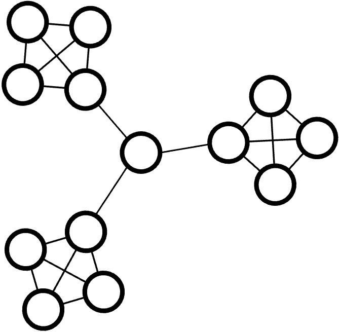
Figure 1: Sachdeva star with $l=3$ and $k=4$.

Results are shown in Table 1. This is the most challenging problem for AC. The iteration counts of AC spiked when compared to other problems. This suggests that AC failed to produce reliable factorizations for the Sachdeva star Laplacians. In contrast, AC2 produced much more reliable factorizations and the iteration counts are still comparable to other problems of similar sizes. In Section 5.5 we have a more detailed comparison between variants of our approximate Cholesky solvers on Sachdeva star. We observe that CMG performs the best for this problem, while HyPre, PETSc and ICC failed to achieve the desired tolerance on most instances.

[H] $k$ nonzeros variables AC AC2 CMG $\operatorname{nnz}$ $n$ $N_{\text{iter}}$ $t_{\text{solve}}/\operatorname{nnz}$ $t_{\text{total}}/\operatorname{nnz}$ res. err. $N_{\text{iter}}$ $t_{\text{solve}}/\operatorname{nnz}$ $t_{\text{total}}/\operatorname{nnz}$ res. err. $N_{\text{iter}}$ $t_{\text{solve}}/\operatorname{nnz}$ $t_{\text{total}}/\operatorname{nnz}$ res. err. $(K)$ $(K)$ $(\mu s)$ $(\mu s)$ $(10^{-8})$ $(\mu s)$ $(\mu s)$ $(10^{-8})$ $(\mu s)$ $(\mu s)$ $(10^{-8})$ $100$ $500$ $5$ $83$ $0.226$ $0.398$ $0.9$ $28$ $0.0793$ $0.478$ $0.64$ $7$ $0.431$ $0.868$ $3.85\text{\times}{10}^{-06}$ $150$ $1690$ $11$ $149$ $0.502$ $0.748$ $0.96$ $34$ $0.117$ $0.581$ $0.632$ $7$ $0.181$ $0.486$ $2.46\text{\times}{10}^{-06}$ $200$ $4000$ $20$ $167$ $0.682$ $0.931$ $0.955$ $37$ $0.155$ $0.716$ $0.877$ $7$ $0.124$ $0.405$ $1.56\text{\times}{10}^{-06}$ $250$ $7810$ $31$ $241$ $1.07$ $1.43$ $0.998$ $38$ $0.169$ $0.703$ $0.98$ $7$ $0.107$ $0.442$ $1.09\text{\times}{10}^{-06}$ $300$ $13\,500$ $45$ $289$ $1.33$ $1.59$ $0.88$ $39$ $0.179$ $0.719$ $0.854$ $7$ $0.0962$ $0.436$ $8.87\text{\times}{10}^{-07}$ $350$ $21\,400$ $61$ $355$ $1.65$ $1.97$ $0.99$ $40$ $0.188$ $0.733$ $0.996$ $7$ $0.0905$ $0.426$ $8.18\text{\times}{10}^{-07}$ $400$ $32\,000$ $80$ $459$ $2.12$ $2.44$ $0.967$ $40$ $0.186$ $0.718$ $0.985$ $7$ $0.0884$ $0.423$ $8.17\text{\times}{10}^{-07}$ $450$ $45\,600$ $101$ $486$ $2.27$ $2.58$ $0.999$ $43$ $0.202$ $0.745$ $0.902$ $7$ $0.0848$ $0.418$ $6.6\text{\times}{10}^{-07}$ $500$ $62\,500$ $125$ $452$ $2.08$ $2.4$ $0.944$ $43$ $0.198$ $0.747$ $0.808$ $7$ $0.0833$ $0.415$ $6.01\text{\times}{10}^{-07}$ $550$ $83\,200$ $151$ $149$ $0.698$^** $1.02$^** $1.88\text{\times}{10}^{04}$ $41$ $0.192$ $0.753$ $0.792$ $7$ $0.0826$ $0.417$ $1.83\text{\times}{10}^{-06}$ $600$ $108\,000$ $180$ $773$ $3.55$ $3.93$ $0.997$ $45$ $0.208$ $0.849$ $0.741$ $7$ $0.0821$ $0.415$ $5.94\text{\times}{10}^{-07}$ $650$ $137\,000$ $211$ $953$ $4.43$^* $4.76$^* $2.4$ $44$ $0.201$ $1.04$ $0.687$ $7$ $0.0823$ $0.41$ $1.3\text{\times}{10}^{-06}$ $700$ $172\,000$ $245$ $478$ $2.19$^* $2.62$^* $126$ $45$ $0.207$ $0.859$ $0.882$ $7$ $0.0823$ $0.412$ $8.1\text{\times}{10}^{-07}$ $750$ $211\,000$ $281$ $905$ $4.15$^* $4.47$^* $2.33$ $43$ $0.198$ $0.855$ $0.916$ $7$ $0.0813$ $0.409$ $1.41\text{\times}{10}^{-06}$ $800$ $256\,000$ $320$ $669$ $3.07$^* $3.39$^* $32.9$ $45$ $0.207$ $0.883$ $0.956$ $7$ $0.0812$ $0.408$ $1.35\text{\times}{10}^{-06}$ $k$ nonzeros variables HyPre PETSc ICC $\operatorname{nnz}$ $n$ $N_{\text{iter}}$ $t_{\text{solve}}/\operatorname{nnz}$ $t_{\text{total}}/\operatorname{nnz}$ res. err. $N_{\text{iter}}$ $t_{\text{solve}}/\operatorname{nnz}$ $t_{\text{total}}/\operatorname{nnz}$ res. err. $N_{\text{iter}}$ $t_{\text{solve}}/\operatorname{nnz}$ $t_{\text{total}}/\operatorname{nnz}$ res. err. $(K)$ $(K)$ $(\mu s)$ $(\mu s)$ $(10^{-8})$ $(\mu s)$ $(\mu s)$ $(10^{-8})$ $(\mu s)$ $(\mu s)$ $(10^{-8})$ $100$ $500$ $5$ $100$ $0.44$^* $0.84$^* $225$ $2$ $0.032$^** $1.08$^** $2.76\text{\times}{10}^{04}$ Inf Inf Inf $1\text{\times}{10}^{08}$ $150$ $1690$ $11$ $100$ $0.45$^* $0.995$^* $493$ $2$ $0.0341$^** $1.47$^** $2.63\text{\times}{10}^{04}$ Inf Inf Inf $1\text{\times}{10}^{08}$ $200$ $4000$ $20$ $100$ $0.692$^* $1.4$^* $2.87\text{\times}{10}^{03}$ $2$ $0.0376$^** $1.93$^** $2.09\text{\times}{10}^{04}$ $1$ $0.0789$ $0.168$ $8.83\text{\times}{10}^{-08}$ $250$ $7810$ $31$ $100$ $0.852$^* $1.73$^* $15.2$ $1$ $0.041$^** $2.37$^** $1.68\text{\times}{10}^{04}$ $1$ $0.0475$ $0.146$ $9.52\text{\times}{10}^{-08}$ $300$ $13\,500$ $45$ $100$ $0.849$^** $1.89$^** $3.91\text{\times}{10}^{04}$ $2$ $0.0427$^** $2.81$^** $1.56\text{\times}{10}^{04}$ $1$ $0.0316$ $0.14$ $1.02\text{\times}{10}^{-07}$ $350$ $21\,400$ $61$ $100$ $0.855$^** $2.07$^** $1.14\text{\times}{10}^{06}$ $5$ $0.106$^* $3.31$^* $4.21\text{\times}{10}^{03}$ Inf Inf Inf $1\text{\times}{10}^{08}$ $400$ $32\,000$ $80$ $100$ $0.842$^* $2.22$^* $1.54\text{\times}{10}^{03}$ $1$ $0.0394$^** $3.69$^** $1.2\text{\times}{10}^{04}$ $1$ $0.022$ $0.151$ $1.3\text{\times}{10}^{-07}$ $450$ $45\,600$ $101$ $100$ $0.852$^** $2.4$^** $2.71\text{\times}{10}^{06}$ $2$ $0.0388$^** $4.13$^** $1.21\text{\times}{10}^{04}$ $1$ $0.0202$ $0.163$ $1.32\text{\times}{10}^{-07}$ $500$ $62\,500$ $125$ $100$ $0.848$^** $2.55$^** $1.47\text{\times}{10}^{05}$ $1$ $0.0374$^** $4.57$^** $1.03\text{\times}{10}^{04}$ Inf Inf Inf $1\text{\times}{10}^{08}$ $550$ $83\,200$ $151$ $100$ $0.834$^* $2.7$^* $3.36\text{\times}{10}^{03}$ $2$ $0.0371$^* $5.05$^* $9.35\text{\times}{10}^{03}$ $1$ $0.0183$ $0.188$ $1.46\text{\times}{10}^{-07}$ $600$ $108\,000$ $180$ $47$ $0.396$ $2.42$ $0.562$ $2$ $0.0572$^* $5.47$^* $9.17\text{\times}{10}^{03}$ $1$ $0.0177$ $0.2$ $1.51\text{\times}{10}^{-07}$ $650$ $137\,000$ $211$ $100$ $0.831$^* $3.02$^* $4.37\text{\times}{10}^{03}$ $2$ $0.0568$^* $5.93$^* $8.53\text{\times}{10}^{03}$ $1$ $0.0169$ $0.212$ $1.62\text{\times}{10}^{-07}$ $700$ $172\,000$ $245$ $100$ $0.831$^* $3.19$^* $236$ $3$ $0.0567$^* $6.35$^* $8.93\text{\times}{10}^{03}$ Inf Inf Inf $1\text{\times}{10}^{08}$ $750$ $211\,000$ $281$ $100$ $0.828$^** $3.35$^** $5.89\text{\times}{10}^{04}$ $2$ $0.0371$^* $6.77$^* $8.59\text{\times}{10}^{03}$ $1$ $0.0161$ $0.235$ $1.71\text{\times}{10}^{-07}$ $800$ $256\,000$ $320$ $100$ $0.821$^* $3.52$^* $2.44\text{\times}{10}^{03}$ $2$ $0.0388$^* $7.22$^* $8.43\text{\times}{10}^{03}$ Inf Inf Inf $1\text{\times}{10}^{08}$ Sachdeva Star with ($k/2$) Leaves Replaced by Complete Graph on $k$ Vertices

• relative residual error exceeded tolerance $10^{-8}$ by a factor $(1,10^{4}]$.

• relative residual error exceeded tolerance $10^{-8}$ by a factor $(10^{4},10^{8})$.

• Inf: Solver crashed or returned a solution with relative residual error 1 (trivial solution).

• N/A: Experiment omitted as the solver crashed too often with (only occurred for PETSc).

5.3.4 Interior Point Method Matrices

In this section we report the performances of solvers on matrices generated from running an Interior Point Method on undirected Maximum Flow problems on two classes of graphs. Our Maximum Flow interior point solver is based on the [KLS20] framework, and uses too many iterations to be practical. Hence, our main interest is to examine if the resulting linear equations are tractable using various solvers.

IPM on Chimeras.

First, we tested the solvers using Laplacians generated from running a Maximum Flow IPM unweighted on Chimeras (see section 5.3.2 for details on Chimera graphs). We ran the IPM on five Chimeras with $10^{5}$ vertices and with the generating seed index $i$ ranging from $1$ to $5$. We compute and store a number of the Laplacian linear equations encountered during a run of the IPM: Concretely, the IPM has a homotopy parameter, which measure roughly how close we are to having an optimal maximum flow solution. As the algorithm progresses, the homotopy parameter changes and the currently maintained approximate maximum flow solution improves in quality. We collect matrices at five different stages, corresponding to different values of the homotopy parameter, and hence different current solution qualites. First, we collect matrices when the maximum flow solution is guaranteed error at most $10^{-1}$ by the homotopy parameter; then we collect when the guaranteed error is $10^{-2},10^{-3},10^{-4}$ and $10^{-5}$. At each of these five collection stages, we store roughly $5$ Laplacians corresponding to consequtive Newton steps in each precision range, for a total of 25 Laplacians per Maximum Flow problem.

In general, the weights in the Laplacian matrices will get increasingly extreme as the precision parameter decreases (meaning the error is smaller). Thus we might expect the problems to become increasingly difficult as the precision parameter decreases. Table 5.3.4 reports detailed performances of the solvers in each precision range, showing the median, 75th percentile, and worst case running times across the five Chimera instances we tested. “AC”, “AC2”, “CMG” and “ICC” reached the desired tolerance on all instances. “AC” is clearly the fastest solver across precision ranges, while the other solvers still managed a comparable run time. We omitted PETSc because we found it to be very unstable on these IPM-weighted Chimera Laplacians and frequently crashed.

IPM on Spielman graphs.

After our Chimera IPM experiments, we tested a family of graphs called Spielman graphs. These are conjectured to be a hard instance for short-step Maximum Flow IPMs – i.e. short-step IPMs need many Newton steps to converge on graphs. Spielman graphs are built recursively across a number of levels. There is unique Spielman graph with $k$ levels, and it has $O(k^{3})$ vertices and edges. This family has a high degree of symmetry, which allows an algorithm based on implicit representations (which we call R-space representation) of the flow solution to compute intermediate states of the IPM very quickly. We use this to speed up our experiments, by only employing a Laplacian solver at a few points spaced evenly throughout a run of the IPM, and using R-space representation for majority of the Newton steps. We run the IPM up to precision $10^{-6}$. For each number of levels $k=100,200,300,400,500,600$ (or in terms of number of edges of the Spielman graphs: from roughly a million up to $200$ millions), we take roughly $10$ Laplacians that occurs when running Maximum Flow IPM. The Laplacians are distributed evenly across precision ranges include the first and the final Laplacians during each run of the IPM. Table 5.3.4 reports the details of the performances of the solvers on Laplcians from running our Maximum Flow IPM on Spielman graphs. Only “AC”, “AC2” and “HyPre” reached the desired tolerence on all instances. The running time of these three solvers are roughly comparable. The results of this experiment are shown in Table 5.3.4.

[H] IPM param. # instances AC $t_{\text{total}}/\operatorname{nnz}$ AC2 $t_{\text{total}}/\operatorname{nnz}$ CMG $t_{\text{total}}/\operatorname{nnz}$ median 0.75 max median 0.75 max median 0.75 max $(10^{-3})$ $(\mu s)$ $(\mu s)$ $(\mu s)$ $(\mu s)$ $(\mu s)$ $(\mu s)$ $(\mu s)$ $(\mu s)$ $(\mu s)$ $100$ $28$ $0.68$ $0.774$ $1.2$ $1.27$ $1.79$ $2.39$ $1.2$ $1.61$ $1.8$ $10$ $27$ $0.678$ $0.777$ $1.15$ $1.27$ $1.8$ $2.36$ $1.2$ $1.56$ $1.69$ $1$ $27$ $0.68$ $0.763$ $1.14$ $1.25$ $1.79$ $2.38$ $1.21$ $1.66$ $1.78$ $0.1$ $27$ $0.683$ $0.784$ $1.15$ $1.27$ $1.79$ $2.36$ $1.19$ $1.58$ $1.78$ $0.01$ $19$ $0.681$ $0.777$ $1.15$ $1.28$ $1.78$ $2.37$ $1.22$ $1.59$ $1.9$
IPM param. # instances HyPre $t_{\text{total}}/\operatorname{nnz}$ PETSc $t_{\text{total}}/\operatorname{nnz}$ ICC $t_{\text{total}}/\operatorname{nnz}$ median 0.75 max median 0.75 max median 0.75 max $(10^{-3})$ $(\mu s)$ $(\mu s)$ $(\mu s)$ $(\mu s)$ $(\mu s)$ $(\mu s)$ $(\mu s)$ $(\mu s)$ $(\mu s)$ $100$ $28$ $1.54$ $2.27$ $5.04$ N/A N/A N/A $0.857$ $1.19$ $2.84$ $10$ $27$ $1.52$ $2.29$ $4.82$ N/A N/A N/A $0.873$ $1.18$ $2.82$ $1$ $27$ $1.52$ $2.32$ $4.94$^* N/A N/A N/A $0.855$ $1.19$ $2.92$ $0.1$ $27$ $1.53$ $2.29$ $4.86$^* N/A N/A N/A $0.858$ $1.2$ $2.88$ $0.01$ $19$ $1.52$ $2.3$ $4.58$^* N/A N/A N/A $0.851$ $1.19$ $2.91$ Chimera IPM

• relative residual error exceeded tolerance $10^{-8}$ by a factor $(1,10^{4}]$.

• relative residual error exceeded tolerance $10^{-8}$ by a factor $(10^{4},10^{8})$.

• Inf: Solver crashed or returned a solution with relative residual error 1 (trivial solution).

• N/A: Experiment omitted as the solver crashed too often with (only occurred for PETSc).

[H] edges # instances AC $t_{\text{total}}/\operatorname{nnz}$ AC2 $t_{\text{total}}/\operatorname{nnz}$ CMG $t_{\text{total}}/\operatorname{nnz}$ $n$ median 0.75 max median 0.75 max median 0.75 max $(K)$ $(\mu s)$ $(\mu s)$ $(\mu s)$ $(\mu s)$ $(\mu s)$ $(\mu s)$ $(\mu s)$ $(\mu s)$ $(\mu s)$ $1030$ $10$ $0.162$ $0.172$ $0.247$ $0.28$ $0.287$ $0.313$ $1.18$ $1.2$ $1.35$ $8100$ $10$ $0.194$ $0.195$ $0.223$ $0.296$ $0.305$ $0.369$ $1.03$ $1.03$^* $1.07$^** $2.72\text{\times}{10}^{04}$ $10$ $0.229$ $0.25$ $0.286$ $0.346$ $0.354$ $0.389$ $1.26$^* $1.37$^* $1.57$^* $6.44\text{\times}{10}^{04}$ $10$ $0.247$ $0.268$ $0.291$ $0.357$ $0.367$ $0.396$ $1.13$^* $1.35$^* $1.62$^* $1.26\text{\times}{10}^{05}$ $10$ $0.264$ $0.279$ $0.362$ $0.422$ $0.428$ $0.428$ $1.43$ $1.44$^* $1.69$^* $2.17\text{\times}{10}^{05}$ $11$ $0.418$ $0.437$ $0.735$ $0.502$ $0.51$ $0.809$ $1.5$ $1.57$^* $1.74$^*
edges # instances HyPre $t_{\text{total}}/\operatorname{nnz}$ PETSc $t_{\text{total}}/\operatorname{nnz}$ ICC $t_{\text{total}}/\operatorname{nnz}$ $n$ median 0.75 max median 0.75 max median 0.75 max $(K)$ $(\mu s)$ $(\mu s)$ $(\mu s)$ $(\mu s)$ $(\mu s)$ $(\mu s)$ $(\mu s)$ $(\mu s)$ $(\mu s)$ $1030$ $10$ $0.346$ $0.361$ $0.449$ $0.76$ $1.06$ $1.81$^* $3.56$ $3.64$ $3.99$ $8100$ $10$ $0.454$ $0.48$ $1.22$ $1.22$ $1.85$ $3.32$^* Inf Inf Inf $2.72\text{\times}{10}^{04}$ $10$ $0.533$ $0.551$ $0.621$ $1.84$ $2.47$ $2.61$ Inf Inf Inf $6.44\text{\times}{10}^{04}$ $10$ $0.583$ $0.62$ $0.725$ $1.68$ $2.05$ $3.27$ Inf Inf Inf $1.26\text{\times}{10}^{05}$ $10$ $0.633$ $0.665$ $0.768$ $2.38$ $2.6$ $3.24$ Inf Inf Inf $2.17\text{\times}{10}^{05}$ $11$ $0.643$ $0.693$ $0.811$ $2.31$ $2.82$ $3.98$ Inf Inf Inf Maximum Flow IPM Laplacians from Spielman graphs.

• relative residual error exceeded tolerance $10^{-8}$ by a factor $(1,10^{4}]$.

• relative residual error exceeded tolerance $10^{-8}$ by a factor $(10^{4},10^{8})$.

• Inf: Solver crashed or returned a solution with relative residual error 1 (trivial solution).

• N/A: Experiment omitted as the solver crashed too often with (only occurred for PETSc).

5.3.5 SPE Benchmark

In this section, we report the performance of solvers on SDDM matrices from the Society of Petroleum Engineering benchmark [CB01]. Here we made use of the matrices from [CCB⁺20]. These matrices are generated from a $3$D waterflood of a geostatistical model. The problem size ranges from $0.5$M to $16$M.

Results are shown in Table 3. On this problem, CMG and HyPre have particularly good performances and beats other solvers. On the other hand, ICC performed poorly with very large iteration counts for the two largest problem instances. The runtimes of AC2 are very close to that of AC, but again, SPE benchmark is not hard enough for AC2 to out-perform AC.

nonzeros	variables	AC				AC2				CMG
$\operatorname{nnz}$	$n$	$N_{\text{iter}}$	$t_{\text{solve}}/\operatorname{nnz}$	$t_{\text{total}}/\operatorname{nnz}$	res. err.	$N_{\text{iter}}$	$t_{\text{solve}}/\operatorname{nnz}$	$t_{\text{total}}/\operatorname{nnz}$	res. err.	$N_{\text{iter}}$	$t_{\text{solve}}/\operatorname{nnz}$	$t_{\text{total}}/\operatorname{nnz}$	res. err.
$(K)$	$(K)$		$(\mu s)$	$(\mu s)$	$(10^{-8})$		$(\mu s)$	$(\mu s)$	$(10^{-8})$		$(\mu s)$	$(\mu s)$	$(10^{-8})$
$2910$	$422$	$17$	$0.24$	$0.718$	$0.433$	$13$	$0.23$	$1.07$	$0.288$	$13$	$0.222$	$0.436$	$0.504$
$14\,600$	$2100$	$22$	$0.359$	$0.967$	$0.337$	$14$	$0.291$	$1.31$	$0.315$	$14$	$0.184$	$0.363$	$0.679$
$28\,500$	$4100$	$22$	$0.404$	$0.928$	$0.474$	$14$	$0.337$	$1.34$	$0.416$	$15$	$0.194$	$0.364$	$0.884$
$55\,800$	$8000$	$39$	$0.893$	$1.49$	$0.495$	$27$	$0.796$	$1.79$	$0.256$	$25$	$0.336$	$0.51$	$0.744$
$112\,000$	$16\,000$	$41$	$1.03$	$1.62$	$0.331$	$26$	$0.868$	$1.91$	$0.28$	$25$	$0.338$	$0.511$	$0.861$

nonzeros	variables	HyPre				PETSc				ICC
$\operatorname{nnz}$	$n$	$N_{\text{iter}}$	$t_{\text{solve}}/\operatorname{nnz}$	$t_{\text{total}}/\operatorname{nnz}$	res. err.	$N_{\text{iter}}$	$t_{\text{solve}}/\operatorname{nnz}$	$t_{\text{total}}/\operatorname{nnz}$	res. err.	$N_{\text{iter}}$	$t_{\text{solve}}/\operatorname{nnz}$	$t_{\text{total}}/\operatorname{nnz}$	res. err.
$(K)$	$(K)$		$(\mu s)$	$(\mu s)$	$(10^{-8})$		$(\mu s)$	$(\mu s)$	$(10^{-8})$		$(\mu s)$	$(\mu s)$	$(10^{-8})$
$2910$	$422$	$6$	$0.199$	$0.508$	$0.0937$	$9$	$1.63$	$2.38$	$1\text{\times}{10}^{-06}$	$36$	$0.466$	$0.527$	$0.99$
$14\,600$	$2100$	$6$	$0.213$	$0.518$	$0.378$	$9$	$1.71$	$2.46$	$4.33\text{\times}{10}^{-06}$	$57$	$0.588$	$0.683$	$0.999$
$28\,500$	$4100$	$6$	$0.215$	$0.519$	$0.384$	$9$	$1.73$	$2.49$	$5.78\text{\times}{10}^{-06}$	$59$	$0.596$	$0.699$	$0.935$
$55\,800$	$8000$	$10$	$0.34$	$0.646$	$0.287$	$9$	$1.77$	$2.57$	$0.009\,28$	$380$	$4.18$	$4.29$	$0.999$
$112\,000$	$16\,000$	$10$	$0.342$	$0.648$	$0.301$	$9$	$1.78$	$2.58$	$0.009\,39$	$377$	$4.08$	$4.2$	$0.998$

Table 3: SPE Benchmark

5.3.6 Poisson Problems on 3D Domains

We adopt a suite of experiments similar to [SBB⁺12], which evaluated the performance of the HyPre-BoomerAMG algebraic multigrid on discretizations of several Poisson problems, also known as scalar elliptic diffusion problems.

We consider systems of linear equations arising from Poisson problems with Dirichlet boundary conditions on a domain $\Omega$ with a spatially varying scalar diffusion coefficient $\mu$, and consider both the case of $\mu$ isotropic and anisotropic,

$$\begin{cases}\operatorname{div}(\mu(x)\bm{\nabla}u(x))=f(x)&\text{ for all }x\in\Omega\\ u(x)=0&\text{ for }x\in\partial\Omega\end{cases}$$ (26)

We adopt a finite volume method discretization approach similar to [BCK⁺18].

We consider a unit cube domain $\Omega=[0,1]^{3}$ using a standard 3D 7-point stencil. We discretize along three dimensions with $n_{1}$, $n_{2}$, and $n_{3}$ variables spaced evenly along each dimension, leading to a 3D grid with $n=n_{1}\cdot n_{2}\cdot n_{3}$ variables, indexed by $u_{i,j,k}$ with $(i,j,k)\in[n_{1}]\times[n_{2}]\times[n_{3}]$, at positions

$$\left(\frac{i-1}{n_{1}-1},\frac{j-1}{n_{2}-1},\frac{k-1}{n_{3}-1}\right)\in\Omega$$

When a point is on the boundary $\partial\Omega$, we introduce the equation $u_{i,j,k}=0$ (equivalently, we remove the corresponding matrix row and column). When a point is not on the boundary of $\Omega$, we set

$$-(a_{\text{north}}+a_{\text{south}}+a_{\text{east}}+a_{\text{west}}+a_{\text{up}}+a_{\text{down}})u_{i,j,k}$$

$$+a_{\text{north}}u_{i+1,j,k}+a_{\text{south}}u_{i-1,j,k}+a_{\text{east}}u_{i,j+1,k}+a_{\text{west}}u_{i,j-1,k}+a_{\text{up}}u_{i,j,k+1}+a_{\text{down}}u_{i,j,k-1}=f_{i,j,k}$$

where we used $a_{\text{north}}$ to refer to the coefficient $\mu(x)$ at the domain location $x\in\Omega$ halfway between the domain locations of $u_{i,j,k}$ and $u_{i+1,j,k}$ and so on. This discretization scheme directly leads to an SDDM matrix.

Unlike [BCK⁺18], for simplicity, when our domain $\Omega$ has regions with varying diffusion coefficient $\mu$, we ensure these regions are aligned so that there is always a variable on the boundary between regions and the $x\in\Omega$ giving rise to each coefficient $a_{\text{direction}}$ falls entirely in one region. This lets us avoid averaging over different $x$ to obtain our coefficients $a_{\text{direction}}$.

Uniform coefficient 3D cube.

In this experiment, we consider a unit cube domain $\Omega=[0,1]^{3}$ with uniform coefficient $\mu(x)=1$ everywhere and equally fine-grained discretization along each dimension, i.e. $n_{1}=n_{2}=n_{3}$. Results are shown in Table 4. We see that AC2 has slightly better iteration counts on the uniform grid than AC, suggesting that indeed AC2 produced more reliable facorization. ICC in contrast produced the most unreliable factorization, causing its iteration counts to be significantly more than other solvers. HyPre and PETSc have the best iteration counts. However, even though they both use BoomerAMG as the preconditioner, HyPre has better runtime than PETSc.

High-contrast variable coefficient 3D cube.

In this experiment, we consider a unit cube domain $\Omega=[0,1]^{3}$, with equally fine-grained discretization along each dimension, i.e. $n_{1}=n_{2}=n_{3}$. We now adopt a checkboard pattern for the coefficient $\mu$, dividing this into subregions with varying coefficients, similar to experiments in [SBB⁺12, BCK⁺18].

Formally, we divide the $[0,1]^{3}$ into $k$ intervals along each axis, leading to $k^{3}$ smaller cubes, which we refer to as subregions. Each subregion has a fixed $\mu$ value, and we pick these to form a checkerboard pattern. Formally, the checkerboard pattern is given a pattern of for $(x,y,z)\in\Omega$

$$\mu(x,y,z)=\begin{cases}1&\text{ if }\left\lfloor k\cdot x\right\rfloor+\left\lfloor k\cdot z\right\rfloor+\left\lfloor k\cdot y\right\rfloor\equiv 0\pmod{2}\\ w&\text{ otherwise }\end{cases}$$ (27)

Figure 2 shows an example with $k=4$.

Figure 2: Checkered cube domain $\Omega$ following Equation (27) with $k=4$. Black subregions have $\mu(x)=w$, white subregions have $\mu(x)=1$.

Results are shown in Table 5. Experiments showed that high-contrast variable coefficient 3D cube is more difficult than the uniform grid for our solvers. But it is not difficult enough for AC2 to match AC in terms of the runtime. Again, ICC produced the most unreliable factorization and consequently the worst iteration count. CMG and HyPre on the other hand maintained roughly the same level of iteration count and runtime as for the uniform grid.

nonzeros	variables	AC				AC2				CMG
$\operatorname{nnz}$	$n$	$N_{\text{iter}}$	$t_{\text{solve}}/\operatorname{nnz}$	$t_{\text{total}}/\operatorname{nnz}$	res. err.	$N_{\text{iter}}$	$t_{\text{solve}}/\operatorname{nnz}$	$t_{\text{total}}/\operatorname{nnz}$	res. err.	$N_{\text{iter}}$	$t_{\text{solve}}/\operatorname{nnz}$	$t_{\text{total}}/\operatorname{nnz}$	res. err.
$(K)$	$(K)$		$(\mu s)$	$(\mu s)$	$(10^{-8})$		$(\mu s)$	$(\mu s)$	$(10^{-8})$		$(\mu s)$	$(\mu s)$	$(10^{-8})$
$1990$	$287$	$24$	$0.319$	$0.769$	$0.524$	$18$	$0.32$	$1.17$	$0.739$	$27$	$0.422$	$0.602$	$0.815$
$19\,900$	$2860$	$25$	$0.453$	$1.07$	$0.913$	$20$	$0.549$	$1.74$	$0.472$	$27$	$0.423$	$0.537$	$0.773$
$200\,000$	$28\,700$	$27$	$0.833$	$1.46$	$0.612$	$20$	$0.99$	$2.49$	$0.679$	$27$	$0.509$	$0.624$	$0.982$

nonzeros	variables	HyPre				PETSc				ICC
$\operatorname{nnz}$	$n$	$N_{\text{iter}}$	$t_{\text{solve}}/\operatorname{nnz}$	$t_{\text{total}}/\operatorname{nnz}$	res. err.	$N_{\text{iter}}$	$t_{\text{solve}}/\operatorname{nnz}$	$t_{\text{total}}/\operatorname{nnz}$	res. err.	$N_{\text{iter}}$	$t_{\text{solve}}/\operatorname{nnz}$	$t_{\text{total}}/\operatorname{nnz}$	res. err.
$(K)$	$(K)$		$(\mu s)$	$(\mu s)$	$(10^{-8})$		$(\mu s)$	$(\mu s)$	$(10^{-8})$		$(\mu s)$	$(\mu s)$	$(10^{-8})$
$1990$	$287$	$7$	$0.201$	$0.488$	$0.197$	$5$	$0.62$	$1.62$	$0.004\,02$	$61$	$0.694$	$0.765$	$0.917$
$19\,900$	$2860$	$8$	$0.259$	$0.572$	$0.113$	$5$	$0.771$	$2.02$	$0.005\,18$	$109$	$1.09$	$1.19$	$0.974$
$200\,000$	$28\,700$	$7$	$0.235$	$0.587$	$0.206$	$6$	$1.01$	$2.62$	$0.000\,333$	$187$	$2.08$	$2.22$	$0.973$

Table 4: Uniform coefficient 3D cube

axis intervals	AC				AC2				CMG
$k$	$N_{\text{iter}}$	$t_{\text{solve}}/\operatorname{nnz}$	$t_{\text{total}/\operatorname{nnz}}$	res. err.	$N_{\text{iter}}$	$t_{\text{solve}}/\operatorname{nnz}$	$t_{\text{total}/\operatorname{nnz}}$	res. err.	$N_{\text{iter}}$	$t_{\text{solve}}/\operatorname{nnz}$	$t_{\text{total}/\operatorname{nnz}}$	res. err.
		$(\mu s)$	$(\mu s)$	$(10^{-8})$		$(\mu s)$	$(\mu s)$	$(10^{-8})$		$(\mu s)$	$(\mu s)$	$(10^{-8})$
$2$	$41$	$1.28$	$1.88$	$0.742$	$30$	$1.48$	$3.01$	$0.987$	$28$	$0.422$	$0.539$	$0.588$
$4$	$47$	$1.47$	$2.1$	$0.733$	$35$	$1.74$	$3.14$	$0.786$	$28$	$0.436$	$0.553$	$0.781$
$8$	$52$	$1.61$	$2.24$	$0.836$	$38$	$1.87$	$3.26$	$0.985$	$27$	$0.425$	$0.551$	$0.745$
$16$	$52$	$1.57$	$2.19$	$0.915$	$46$	$2.2$	$3.57$	$0.707$	$28$	$0.446$	$0.572$	$0.834$
$32$	$59$	$1.73$	$2.33$	$0.802$	$45$	$2.06$	$3.38$	$0.967$	$28$	$0.399$	$0.534$	$0.867$
$64$	$57$	$1.59$	$2.16$	$0.925$	$48$	$2.02$	$3.23$	$0.762$	$23$	$0.383$	$0.511$	$0.952$
$128$	$53$	$1.39$	$1.94$	$0.98$	$35$	$1.31$	$2.46$	$0.828$	$26$	$0.403$	$0.541$	$0.907$

axis intervals	HyPre				PETSc				ICC
k	$N_{\text{iter}}$	$t_{\text{solve}}/\operatorname{nnz}$	$t_{\text{total}/\operatorname{nnz}}$	res. err.	$N_{\text{iter}}$	$t_{\text{solve}}/\operatorname{nnz}$	$t_{\text{total}/\operatorname{nnz}}$	res. err.	$N_{\text{iter}}$	$t_{\text{solve}}/\operatorname{nnz}$	$t_{\text{total}/\operatorname{nnz}}$	res. err.
		$(\mu s)$	$(\mu s)$	$(10^{-8})$		$(\mu s)$	$(\mu s)$	$(10^{-8})$		$(\mu s)$	$(\mu s)$	$(10^{-8})$
$2$	$8$	$0.265$	$0.616$	$0.308$	$7$	$1.35$	$3.12$	$0.000\,145$	$175$	$1.94$	$2.09$	$0.968$
$4$	$8$	$0.264$	$0.656$	$0.738$	$7$	$1.65$	$3.79$	$0.000\,555$	$244$	$2.69$	$2.84$	$0.985$
$8$	$9$	$0.295$	$0.734$	$0.351$	$7$	$1.77$	$3.85$	$0.001\,42$	$323$	$3.54$	$3.68$	$0.982$
$16$	$9$	$0.289$	$0.752$	$0.184$	$8$	$1.95$	$3.84$	$0.000\,297$	$351$	$3.84$	$3.99$	$0.979$
$32$	$8$	$0.257$	$0.732$	$0.744$	$8$	$1.83$	$3.43$	$0.001\,17$	$343$	$3.77$	$3.92$	$0.952$
$64$	$8$	$0.258$	$0.64$	$0.513$	$9$	$1.43$	$2.35$	$0.000\,498$	$383$	$4.19$	$4.33$	$0.958$
$128$	$7$	$0.244$	$0.55$	$0.98$	$7$	$0.664$	$1.1$	$0.001\,06$	$420$	$4.61$	$4.76$	$0.994$

Table 5: High-contrast variable coefficient 3D cube. Unit cube domain with $\Omega=[0,1]^{3}$, with equally fine-grained discretization along each dimension. 28.7 M variables and 200 M non-zeros. Weight $w=10^{7}$. Times are reported in seconds.

aniso. stretch	nonzeros	variables	AC				AC2				CMG
$\eta$	$\operatorname{nnz}$	$n$	$N_{\text{iter}}$	$t_{\text{solve}}/\operatorname{nnz}$	$t_{\text{total}}/\operatorname{nnz}$	res. err.	$N_{\text{iter}}$	$t_{\text{solve}}/\operatorname{nnz}$	$t_{\text{total}}/\operatorname{nnz}$	res. err.	$N_{\text{iter}}$	$t_{\text{solve}}/\operatorname{nnz}$	$t_{\text{total}}/\operatorname{nnz}$	res. err.
	$(M)$	$(M)$		$(\mu s)$	$(\mu s)$	$(10^{-8})$		$(\mu s)$	$(\mu s)$	$(10^{-8})$		$(\mu s)$	$(\mu s)$	$(10^{-8})$
$0.001$	$203$	$29.6$	$26$	$0.637$	$1.16$	$0.661$	$19$	$0.729$	$1.99$	$0.871$	$25$	$0.39$	$0.512$	$0.929$
$0.01$	$200$	$28.8$	$26$	$0.724$	$1.32$	$0.904$	$20$	$0.864$	$2.26$	$0.592$	$26$	$0.521$	$0.644$	$0.655$
$0.1$	$200$	$28.7$	$27$	$0.809$	$1.42$	$0.618$	$20$	$0.956$	$2.42$	$0.681$	$26$	$0.543$	$0.659$	$0.712$
$1$	$200$	$28.7$	$26$	$0.811$	$1.44$	$0.906$	$20$	$0.994$	$2.5$	$0.753$	$27$	$0.508$	$0.624$	$0.982$
$10$	$200$	$28.7$	$27$	$0.858$	$1.48$	$0.635$	$20$	$0.991$	$2.47$	$0.61$	$28$	$0.513$	$0.629$	$0.708$
$100$	$196$	$28.6$	$25$	$0.741$	$1.31$	$0.845$	$19$	$0.837$	$2.12$	$0.842$	$28$	$0.516$	$0.637$	$0.635$
$1000$	$189$	$29.9$	$23$	$0.494$	$0.956$	$0.733$	$18$	$0.502$	$1.39$	$0.454$	$15$	$0.283$	$0.416$	$0.333$

aniso. stretch	nonzeros	variables	HyPre				PETSc				ICC
$\eta$	$\operatorname{nnz}$	$n$	$N_{\text{iter}}$	$t_{\text{solve}}/\operatorname{nnz}$	$t_{\text{total}}/\operatorname{nnz}$	res. err.	$N_{\text{iter}}$	$t_{\text{solve}}/\operatorname{nnz}$	$t_{\text{total}}/\operatorname{nnz}$	res. err.	$N_{\text{iter}}$	$t_{\text{solve}}/\operatorname{nnz}$	$t_{\text{total}}/\operatorname{nnz}$	res. err.
	$(M)$	$(M)$		$(\mu s)$	$(\mu s)$	$(10^{-8})$		$(\mu s)$	$(\mu s)$	$(10^{-8})$		$(\mu s)$	$(\mu s)$	$(10^{-8})$
$0.001$	$203$	$29.6$	$7$	$0.222$	$0.589$	$0.192$	$5$	$0.677$	$1.62$	$0.003\,66$	$47$	$0.531$	$0.603$	$0.955$
$0.01$	$200$	$28.8$	$7$	$0.228$	$0.583$	$0.2$	$5$	$0.732$	$1.84$	$0.004\,56$	$81$	$0.892$	$0.985$	$0.959$
$0.1$	$200$	$28.7$	$7$	$0.234$	$0.581$	$0.204$	$5$	$0.808$	$2.15$	$0.006\,18$	$129$	$1.43$	$1.54$	$0.999$
$1$	$200$	$28.7$	$7$	$0.235$	$0.587$	$0.205$	$6$	$1.01$	$2.6$	$0.000\,371$	$160$	$1.77$	$1.92$	$0.987$
$10$	$200$	$28.7$	$8$	$0.261$	$0.614$	$0.103$	$5$	$0.638$	$1.77$	$0.004\,14$	$101$	$1.13$	$1.27$	$0.943$
$100$	$196$	$28.6$	$7$	$0.223$	$0.574$	$0.187$	$4$	$0.494$	$1.52$	$0.116$	$35$	$0.401$	$0.53$	$0.752$
$1000$	$189$	$29.9$	$7$	$0.194$	$0.476$	$0.0744$	$4$	$0.545$	$1.41$	$0.002\,11$	$12$	$0.153$	$0.285$	$0.651$

Table 6: Anisotropic coefficient 3D cube with variable discretization and fixed weight.

weight	AC				AC2				CMG
$\eta$	$N_{\text{iter}}$	$t_{\text{solve}}/\operatorname{nnz}$	$t_{\text{total}}/\operatorname{nnz}$	res. err.	$N_{\text{iter}}$	$t_{\text{solve}}/\operatorname{nnz}$	$t_{\text{total}}/\operatorname{nnz}$	res. err.	$N_{\text{iter}}$	$t_{\text{solve}}/\operatorname{nnz}$	$t_{\text{total}}/\operatorname{nnz}$	res. err.
		$(\mu s)$	$(\mu s)$	$(10^{-8})$		$(\mu s)$	$(\mu s)$	$(10^{-8})$		$(\mu s)$	$(\mu s)$	$(10^{-8})$
$0.001$	$39$	$1.09$	$1.67$	$0.902$	$25$	$1.09$	$2.48$	$0.657$	$24$	$0.486$	$0.601$	$0.952$
$0.01$	$33$	$0.951$	$1.53$	$0.944$	$23$	$0.997$	$2.41$	$0.963$	$24$	$0.492$	$0.608$	$0.775$
$0.1$	$26$	$0.778$	$1.37$	$0.992$	$20$	$0.925$	$2.39$	$0.645$	$24$	$0.492$	$0.608$	$0.776$
$1$	$26$	$0.814$	$1.52$	$0.952$	$20$	$0.991$	$2.5$	$0.846$	$27$	$0.503$	$0.619$	$0.972$
$10$	$20$	$0.571$	$1.21$	$0.818$	$15$	$0.63$	$1.95$	$0.413$	$25$	$0.512$	$0.638$	$0.757$
$100$	$17$	$0.399$	$0.916$	$0.464$	$12$	$0.378$	$1.51$	$0.612$	$27$	$0.551$	$0.674$	$0.893$
$1000$	$14$	$0.302$	$0.78$	$0.814$	$10$	$0.257$	$1.05$	$0.91$	$27$	$0.507$	$0.625$	$0.95$

weight	HyPre				PETSc				ICC
$\eta$	$N_{\text{iter}}$	$t_{\text{solve}}/\operatorname{nnz}$	$t_{\text{total}}/\operatorname{nnz}$	res. err.	$N_{\text{iter}}$	$t_{\text{solve}}/\operatorname{nnz}$	$t_{\text{total}}/\operatorname{nnz}$	res. err.	$N_{\text{iter}}$	$t_{\text{solve}}/\operatorname{nnz}$	$t_{\text{total}}/\operatorname{nnz}$	res. err.
		$(\mu s)$	$(\mu s)$	$(10^{-8})$		$(\mu s)$	$(\mu s)$	$(10^{-8})$		$(\mu s)$	$(\mu s)$	$(10^{-8})$
$0.001$	$7$	$0.297$	$0.662$	$0.165$	$6$	$0.621$	$1.16$	$0.000\,816$	$207$	$2.29$	$2.44$	$0.981$
$0.01$	$7$	$0.299$	$0.683$	$0.159$	$6$	$0.733$	$1.38$	$0.000\,871$	$189$	$2.09$	$2.24$	$0.967$
$0.1$	$8$	$0.321$	$0.772$	$0.134$	$7$	$2.76$	$4.92$	$0.008\,65$	$168$	$1.86$	$2.01$	$0.969$
$1$	$7$	$0.235$	$0.588$	$0.207$	$5$	$0.861$	$2.46$	$0.005\,81$	$174$	$1.93$	$2.08$	$0.995$
$10$	$7$	$0.323$	$0.625$	$0.618$	$5$	$1.09$	$2.56$	$0.0704$	$149$	$1.65$	$1.8$	$0.966$
$100$	$8$	$0.282$	$0.449$	$0.34$	$5$	$0.629$	$1.05$	$0.0317$	$77$	$0.867$	$1.02$	$0.928$
$1000$	$7$	$0.223$	$0.332$	$0.128$	$6$	$0.644$	$0.904$	$0.000\,392$	$30$	$0.346$	$0.495$	$0.892$

Table 7: Anisotropic coefficient 3D cube with fixed discretization and variable weight. 28.7 M variables and 200 M non-zeros

Anisotropic coefficient 3D cube with variable discretization and fixed weight.

In this experiment, we follow [SBB⁺12], and study anisotropic coefficient diffusion problems on a unit cube domain $\Omega=[0,1]^{3}$. We include this experiment as [SBB⁺12] highlighted it as a problematic case for Algebraic Multridgrid methods.

We consider systems of linear equations arising from Poisson problems with Dirichlet boundary conditions on a domain $\Omega$ with a fixed matrix coefficient $\mu$. We choose $\mu\in R^{3\times 3}$ as a diagonal matrix with $\mu(1,1)=w$ and $\mu(2,2)=\mu(3,3)=1$.

$$\begin{cases}\operatorname{div}(\mu\bm{\nabla}u(x))=f(x)&\text{ for all }x\in\Omega\\ u(x)=0&\text{ for }x\in\partial\Omega\end{cases}$$ (28)

This is equivalent to the continuous uniform scalar coefficient problem, studied on a rectangular domain $\Omega=[0,1/w]\times[0,1]^{2}$ with equally fine-grained discretization along each dimension.

Our discrete matrix is a grid non-zero structure with uniform weights, symmetric diagonally dominant with negative off-diagonals (SDDM), but we vary the discretization level along each dimension. Concretely, we stretch or shrink the grid along the first dimension by a factor $\eta=1/w$ so that the number of variables along each, denoted $n_{1},n_{2},n_{3}$ satisfy $n_{1}=\eta n_{2}=\eta n_{3}$.

Results are shown in Table 6. Experiments suggest that this is an easier problem than the high-contrast variable coefficient 3D cube for many of the solvers. The performances of the solvers are roughly comparable to their performances on the uniform grid for different discretizations, with the noticeable exception of ICC and PETSc, which performed significantly better for grids with more extreme stretch.

Anisotropic coefficient 3D cube with fixed discretization and variable weight.

We again study the continuous problem from Equation (28), as in the previous experiment. But in this experiment, we discretize equally fine-grained along each axis. This results in a discrete 3D grid, with weights along the first axis of $w$ and weights along the second two axes of $1$, and all three axes having the same number of variables, denoted $n_{1},n_{2},n_{3}$ and satisfying $n_{1}=n_{2}=n_{3}$.

Results are shown in Table 7. For this problem, both AC, AC2 and ICC achieved noticeably lower iteration counts and runtime for weights 100 and 1000, but not for their reciprocal. CMG, HyPre and PETSc again maintained roughly similar performances as for uniform grids.

5.4 Variation in the Performance of our Solvers

In this section, we report the statistics on the variation in the performance of our solvers AC and AC2) (i.e. AC-s2m2). We evaluate the variation in the performance of these solvers with a weighted Chimera with 10 million variables, a weighted SDDM Chimera with 10 million variables, the Sachdeva Star with parameter $k=700$, high contrast coefficient Poisson grid with $200$ million non-zeros and axis interval $32$, and Anisotropic coefficient Poisson grid with fixed discretization and weight $0.001$. For each system of linear equations, we run each solver 10 times.

Results are shown in Table 5.4. Experiments showed that our solvers’ solve time and total time is tightly concentrated, with the only exception occurring with AC on Sachdeva star. This is because AC failed to produce reliable factorizations for Sachdeva stars. In comparison, AC-s2m2 still manage to exhibit a very small variance of runtime on Sachdeva star.

[H] Instance non-zeros AC $t_{\text{solve}}/\operatorname{nnz}$ AC2 (ac-s2m2) $t_{\text{solve}}/\operatorname{nnz}$ AC $t_{\text{total}}/\operatorname{nnz}$ AC2 (ac-s2m2) $t_{\text{total}}/\operatorname{nnz}$ nnz median 0.75 max median 0.75 max median 0.75 max median 0.75 max $(M)$ $\mu s$ $\mu s$ $\mu s$ $\mu s$ $\mu s$ $\mu s$ $\mu s$ $\mu s$ $\mu s$ $\mu s$ $\mu s$ $\mu s$ Weighted chimera $50.2$ $3.78$ $3.87$ $3.95$ $2.59$ $2.6$ $2.68$ $4.65$ $4.74$ $4.82$ $4.09$ $4.11$ $4.18$ Weighted SDDM chimera $49.7$ $3.3$ $3.38$ $3.48$ $2.44$ $2.5$ $2.58$ $4.45$ $4.53$ $4.64$ $4.26$ $4.33$ $4.4$ Sachdeva Star $172$ $2.56$^* $3.52$^** $4.05$^** $0.208$ $0.212$ $0.214$ $2.96$^* $3.86$^** $4.37$^** $0.977$ $0.982$ $0.986$ High contrast coefficient Poisson grid $200$ $1.71$ $1.73$ $1.77$ $2.14$ $2.15$ $2.25$ $2.6$ $2.62$ $2.66$ $3.34$ $3.35$ $3.45$ Anisotropic coef. Poisson grid, variable weight $200$ $1.12$ $1.14$ $1.18$ $1.15$ $1.16$ $1.2$ $1.72$ $1.75$ $1.82$ $2.33$ $2.34$ $2.38$ Variation in total time and solve time of ac and ac-s2m2 computed across 10 runs per system of linear equations.

• relative residual error exceeded tolerance $10^{-8}$ by a factor $(1,10^{4}]$.

• relative residual error exceeded tolerance $10^{-8}$ by a factor $(10^{4},10^{8})$.

• Inf: Solver crashed or returned a solution with relative residual error 1 (trivial solution).

• N/A: Experiment omitted as the solver crashed too often with (only occurred for PETSc).

5.5 Comparison of Algorithm Variants: Splitting and Merging

In this section, we report some further experimental statistics on the qualities of all variants of the approximate Cholesky factorization on the difficult problems described earlier. The factorizations reported here are

• Approximate Cholesky without splitting and with merging of multi-edges down to 1 copy (AC).

• Approximate Cholesky without splitting and without merging (AC-s1).

• Approximate Cholesky with the original edges split into $2$ and without merging (AC-s2).

• Approximate Cholesky with the original edges split into $2$ and merging multi-edges down to $2$ copies (AC-s2m2).

• Approximate Cholesky with the original edges split into $3$ and merging multi-edges down to $3$ copies (AC-s3m3).

For these factorizations, we report the following statistics:

• Total time to solve each linear equation, normalized by non-zero count.

• Condition number of the SDDM matrix and the approximate factorizations. This captures the quality of approximate factorizations.

• Ratio between the size of the output factorization and the input Laplacian (adjacency) matrix.

Results are shown in Table 5.5. Here we remark that AC and AC-s1 did not achieve the target $10^{-8}$ tolerance on the Sachdeva star when $k=700$. For Sachdeva stars, most sampled edges of our solvers occur within the complete graphs on the leaves, hence causing the ratio between the sizes of output factorizations and input Sachdeva star Laplacians to be close to $1$. We see that the initial splitting plays a very significant role in the quality of the output factorization. AC-s1 produced factorizations that have very large condition numbers relative to the input matrix on Sachdeva star, even though it does not compress any multi-edges created during the elimination. On the other hand, the condition number and iteration counts for AC-s2m2 are still very much comparable to that of AC-s2, despite that it only keeps up to 2 multi-edges. This suggests that allowing no limits on multi-edges does not increase quality much compared to versions that merge, and versions without merging are noticeably slower. AC-s3m3 produced the most reliable factorizations and beats AC-s2 in terms of the runtime, but is not as fast as AC-s2m2.

[H] Instance non-zeros AC AC-s1 AC-s2 nnz $t_{\text{total}}/\operatorname{nnz}$ $N_{\text{iter}}$ Ratio of sizes Condition num. $t_{\text{total}}/\operatorname{nnz}$ $N_{\text{iter}}$ Ratio of sizes Condition num. $t_{\text{total}}/\operatorname{nnz}$ $N_{\text{iter}}$ Ratio of sizes Condition num. $(M)$ $\mu s$ $\mu s$ $\mu s$ Weighted chimera $50.2$ $4.42$ $55$ $3.56$ $87.0$ $6.66$ $49$ $4.53$ $75.9$ $9.58$ $35$ $6.67$ $18.5$ Weighted SDDM chimera $49.7$ $4.3$ $51$ $3.29$ $59.8$ $5.63$ $48$ $3.99$ $75.4$ $7.11$ $31$ $5.81$ $28.1$ Sachdeva Star $172$ $2.2$^* $408$ $1.0$ $9660.0$ $3.13$^* $189$ $1.0$ $3090.0$ $5.97$ $31$ $1.0$ $102.0$ High contrast coefficient Poisson grid $200$ $2.24$ $57$ $2.78$ $60.2$ $3.82$ $55$ $3.44$ $66.8$ $6.32$ $44$ $4.86$ $35.8$ Anisotropic coef. Poisson grid, variable weight $200$ $1.78$ $41$ $2.66$ $24.7$ $3.24$ $32$ $3.2$ $16.3$ $5.73$ $23$ $4.41$ $8.78$ Instance non-zeros AC-s2m2 AC-s3m3 nnz $t_{\text{total}}/\operatorname{nnz}$ $N_{\text{iter}}$ Ratio of sizes Condition num. $t_{\text{total}}/\operatorname{nnz}$ $N_{\text{iter}}$ Ratio of sizes Condition num. $(M)$ $\mu s$ $(\mu s)$ Weighted chimera $50.2$ $4.07$ $33$ $5.32$ $29.7$ $4.9$ $26$ $6.73$ $12.7$ Weighted SDDM chimera $49.7$ $3.99$ $30$ $4.8$ $19.0$ $4.49$ $26$ $6.0$ $14.7$ Sachdeva Star $172$ $0.84$ $44$ $1.0$ $64.6$ $1.15$ $31$ $1.0$ $21.4$ High contrast coefficient Poisson grid $200$ $3.44$ $44$ $3.98$ $37.3$ $4.4$ $38$ $4.92$ $30.4$ Anisotropic coef. Poisson grid, variable weight $200$ $2.33$ $26$ $3.69$ $11.6$ $3.12$ $21$ $4.46$ $7.51$ Comparison between variants of the approximate Cholesky factorization using different multi-edge splitting and merging approaches.

• relative residual error exceeded tolerance $10^{-8}$ by a factor $(1,10^{4}]$.

• relative residual error exceeded tolerance $10^{-8}$ by a factor $(10^{4},10^{8})$.

• Inf: Solver crashed or returned a solution with relative residual error 1 (trivial solution).

• N/A: Experiment omitted as the solver crashed too often with (only occurred for PETSc).

5.6 Comparison of Algorithm Variants: Elimination Order

In this section, we investigate the impact of our approximate greedy elimination ordering (see Section 5.1) compared with a randomized ordering. The use of a completely random ordering was suggested in [KS16] which introduced randomized approximate Gaussian elimination. In [KS16], the random ordering plays a role in the proof that the algorithm produces a good factorization. This paper also showed that one can randomize among the vertices with at most twice the average unweighted degree and still get a provably correct algorithm. In our AC and other solvers, we instead eliminate a vertex with approximately minimum unweighted degree in each round. To understand the impact of this choice, we compare AC with a variant that uses uniformly random elimination order, which we call AC-random.

In our first experiment, we reuse the setup from Section 5.4, i.e. we run the AC-random solver 10 times on each of 5 different systems of linear equations and we report the median, 75th percentile, and maximum solve time, normalized by non-zero count, to compare it with our results for AC. The results of this experiment are shown in Table 5.6.

In our second experiment, we reuse the setup from Section 5.5, i.e. we run the AC-random solver once on each of 5 different systems of linear equations and compute the total solve time per non-zero, the ratio of sizes between the input and the output factorization, and the condition number. The results of this experiment are shown in Table 5.6.

In both experiments, we see that AC outperforms AC-random except on Sachdeva stars, where AC does worse on all parameters. This is not so surprising, as the Sachdeva star is designed to challenge the greedy ordering approach in particular. Concretely, eliminating the central vertex of the Sachdeva star early tends to give worse performance, and the parameters we use for the star are such that the greedy ordering eliminates the central vertex first. The results suggest that our greedy ordering approach generally works well, but perhaps could be improved slightly by adding a little more randomness to the elimination ordering.

[H] Instance non-zeros AC $t_{\text{solve}}/\operatorname{nnz}$ AC-random $t_{\text{solve}}/\operatorname{nnz}$ AC $t_{\text{total}}/\operatorname{nnz}$ AC-random $t_{\text{total}}/\operatorname{nnz}$ nnz median 0.75 max median 0.75 max median 0.75 max median 0.75 max $(M)$ $\mu s$ $\mu s$ $\mu s$ $\mu s$ $\mu s$ $\mu s$ $\mu s$ $\mu s$ $\mu s$ $\mu s$ $\mu s$ $\mu s$ Weighted chimera $50.2$ $3.78$ $3.87$ $3.95$ $2.59$ $2.6$ $2.68$ $4.65$ $4.74$ $4.82$ $4.09$ $4.11$ $4.18$ Weighted SDDM chimera $49.7$ $3.3$ $3.38$ $3.48$ $2.44$ $2.5$ $2.58$ $4.45$ $4.53$ $4.64$ $4.26$ $4.33$ $4.4$ Sachdeva Star $172$ $2.56$^* $3.52$^** $4.05$^** $0.208$ $0.212$ $0.214$ $2.96$^* $3.86$^** $4.37$^** $0.977$ $0.982$ $0.986$ High contrast coefficient Poisson grid $200$ $1.71$ $1.73$ $1.77$ $2.14$ $2.15$ $2.25$ $2.6$ $2.62$ $2.66$ $3.34$ $3.35$ $3.45$ Anisotropic coef. Poisson grid, variable weight $200$ $1.12$ $1.14$ $1.18$ $1.15$ $1.16$ $1.2$ $1.72$ $1.75$ $1.82$ $2.33$ $2.34$ $2.38$ Variation in total time of AC and AC-random computed across 10 runs per system of linear equations.

• relative residual error exceeded tolerance $10^{-8}$ by a factor $(1,10^{4}]$.

• relative residual error exceeded tolerance $10^{-8}$ by a factor $(10^{4},10^{8})$.

• Inf: Solver crashed or returned a solution with relative residual error 1 (trivial solution).

• N/A: Experiment omitted as the solver crashed too often with (only occurred for PETSc).

[H] Instance non-zeros AC AC-random nnz $t_{\text{total}}/\operatorname{nnz}$ $N_{\text{iter}}$ Ratio of sizes Condition num. $t_{\text{total}}/\operatorname{nnz}$ $N_{\text{iter}}$ Ratio of sizes Condition num. $(M)$ $\mu s$ $(\mu s)$ Weighted chimera $50.2$ $4.42$ $55$ $3.56$ $87.0$ $9.64$ $112$ $5.03$ $193.0$ Weighted SDDM chimera $49.7$ $4.3$ $51$ $3.29$ $59.8$ $8.47$ $90$ $5.19$ $487.0$ Sachdeva Star $172$ $2.2$^* $408$ $1.0$ $9660.0$ $1.18$ $210$ $1.0$ $4290.0$ High contrast coefficient Poisson grid $200$ $2.24$ $57$ $2.78$ $60.2$ $9.94$ $145$ $3.56$ $436.0$ Anisotropic coef. Poisson grid, variable weight $200$ $1.78$ $41$ $2.66$ $24.7$ $4.97$ $65$ $3.61$ $176.0$ Comparison between approximate Cholesky factorization with different elimination orders.

• relative residual error exceeded tolerance $10^{-8}$ by a factor $(1,10^{4}]$.

• relative residual error exceeded tolerance $10^{-8}$ by a factor $(10^{4},10^{8})$.

• Inf: Solver crashed or returned a solution with relative residual error 1 (trivial solution).

• N/A: Experiment omitted as the solver crashed too often with (only occurred for PETSc).

5.7 Running Time Scaling with Problem Size

In this section, we summarize the running time scaling with problem size of AC and AC2 across all our experiments. We measure total time including factorization and solve.

We show two different types of plots. Our first plot type displays the total running time in seconds plotted against the number of non-zeros ($\operatorname{nnz}$) of the instances, both on a log scale. We also plot the function ${10^{-8}\operatorname{nnz}\log_{10}(\operatorname{nnz})^{3}}$, which agrees with the asymptotic running time scaling predicted by theory from [KS16]. We caution that we do not have a theoretical analysis that establishes such a running time for AC or AC2. Figure 3 shows this plot for AC, while Figure 5 shows this plot for AC2.

Our second plot type again shows running time in seconds measured relative to the non-zero count of the instance plotted against non-zero count of the instances, with the x-axis on a log scale. We also show the function $\frac{{10^{-8}\operatorname{nnz}\log_{10}(\operatorname{nnz})^{3}}}{\operatorname{nnz}}=10^{-8}\log_{10}(\operatorname{nnz})^{3}$, i.e. the same running time fit as in the previous plots, but here normalized by non-zero count. Figures 4 and Figure 6 show these plots for AC and AC2 respectively.

AC running times.

We first show the running time plots for AC as described in the previous section. We use a blue circle to show successful solves and a red square to show solves that failed to reach the target tolerance. All failed solves occurred on Sachdeva star instances.

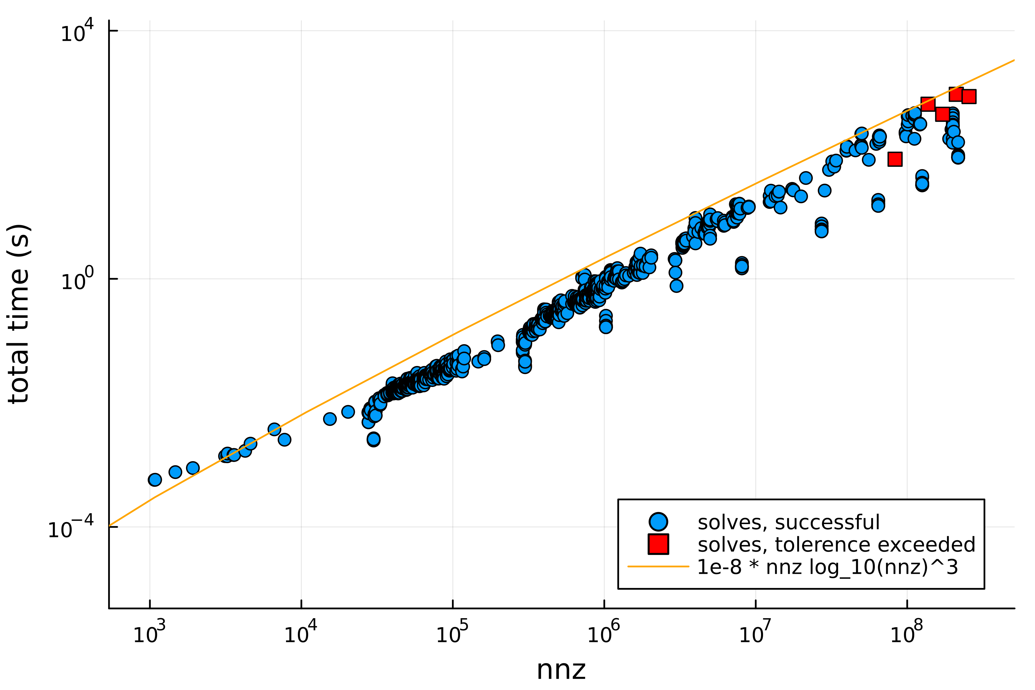
Figure 3: The plot shows data from all our experiments with the AC with total running time in seconds on the y-axis plotted against the number-of-non-zeros of the instance on the x-axis. Solves that reached the target tolerance are shown with a blue circle, while solves that failed to reach tolerance are shown with a red square. An orange line shows the function $\operatorname{nnz}\log_{10}(\operatorname{nnz})^{3}$ (seconds) where $\operatorname{nnz}$ is the non-zero count.

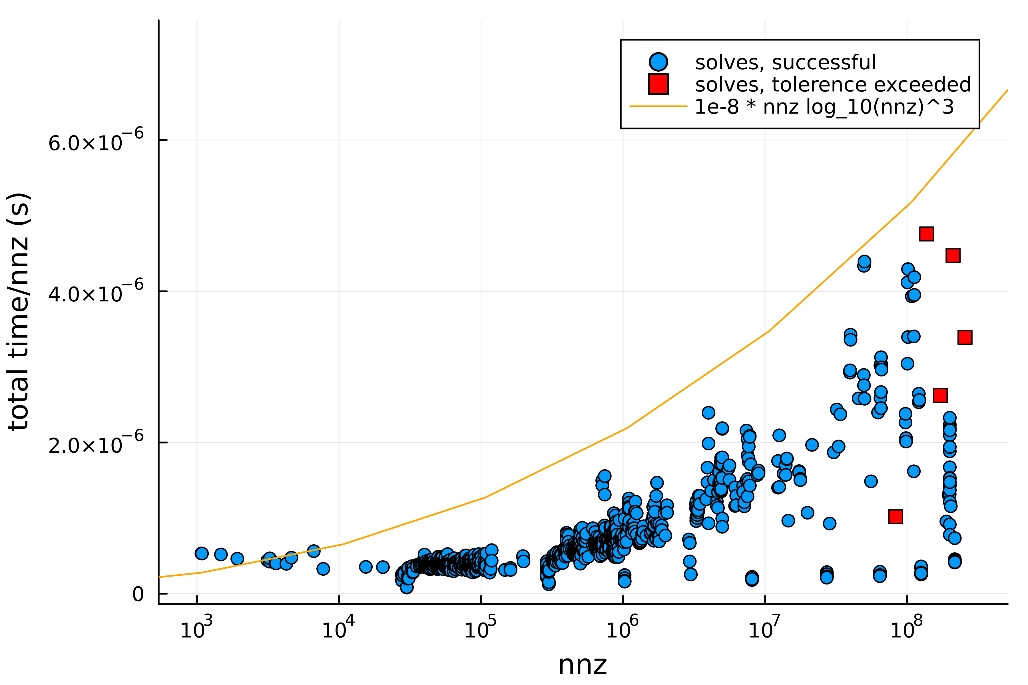
Figure 4: The plot shows data from all our experiments with the AC with total running time per non-zero in seconds on the y-axis plotted against the number-of-non-zeros of the instance on the x-axis. Solves that reached the target tolerance are shown with a blue circle, while solves that failed to reach tolerance are shown with a red square. An orange line shows the function $\operatorname{nnz}\log_{10}(\operatorname{nnz})^{3}$ (seconds) where $\operatorname{nnz}$ is the non-zero count, and the same normalization is used as for the data (i.e. dividing by $\operatorname{nnz}$).

AC2 running times.

We now show running time plots for AC2 as described earlier. We use a blue circle to show successful solves. For AC2, all solves reached the tolerance (i.e. $10^{-8}$ relative residual error).

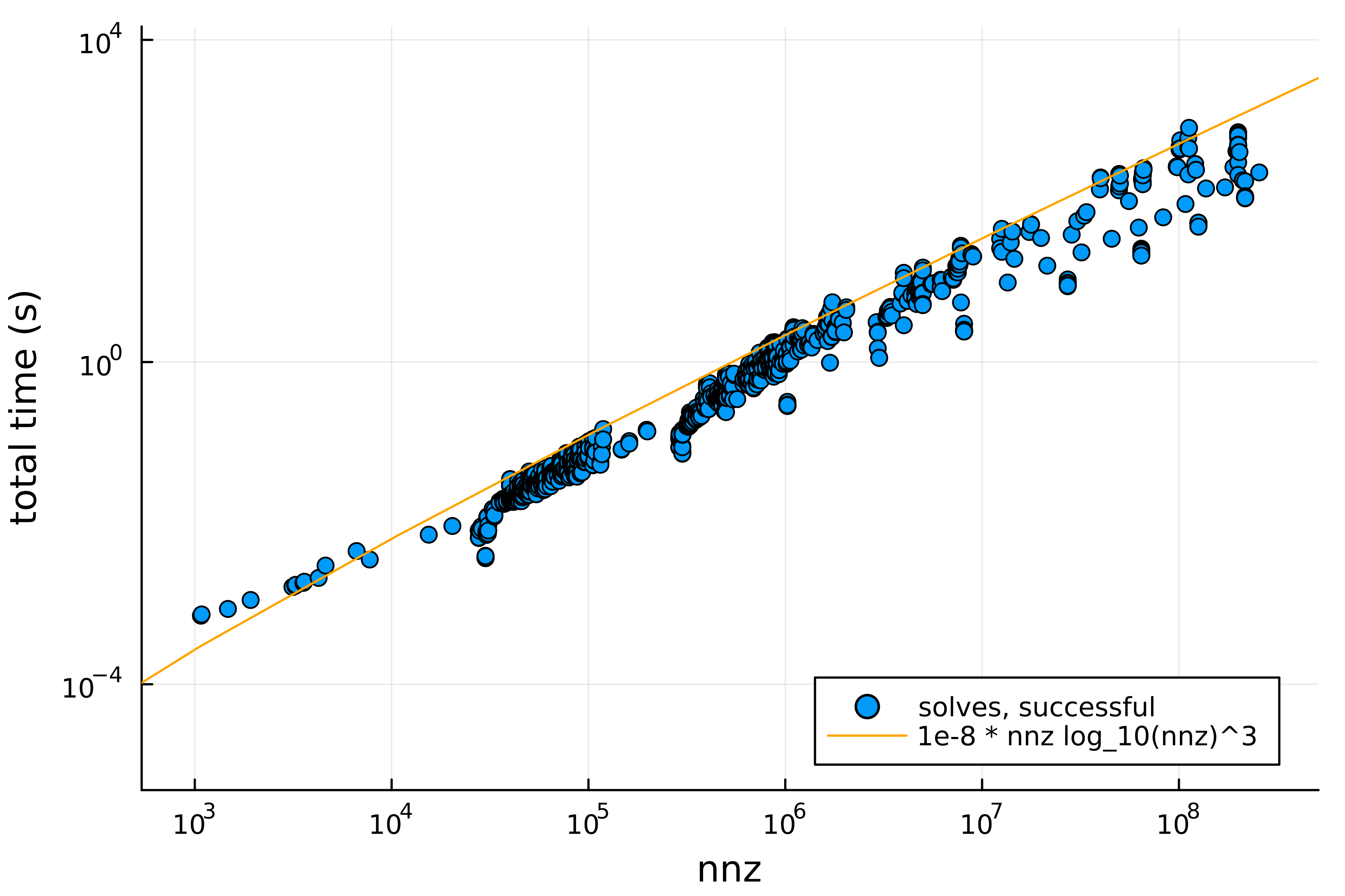
Figure 5: The plot shows data from all our experiments with the AC2 with total running time in seconds on the y-axis plotted against the number-of-non-zeros of the instance on the x-axis. Solves are shown with a blue circle. All solves reached the target tolerance. An orange line shows the function $\operatorname{nnz}\log_{10}(\operatorname{nnz})^{3}$ (seconds) where $\operatorname{nnz}$ is the non-zero count.

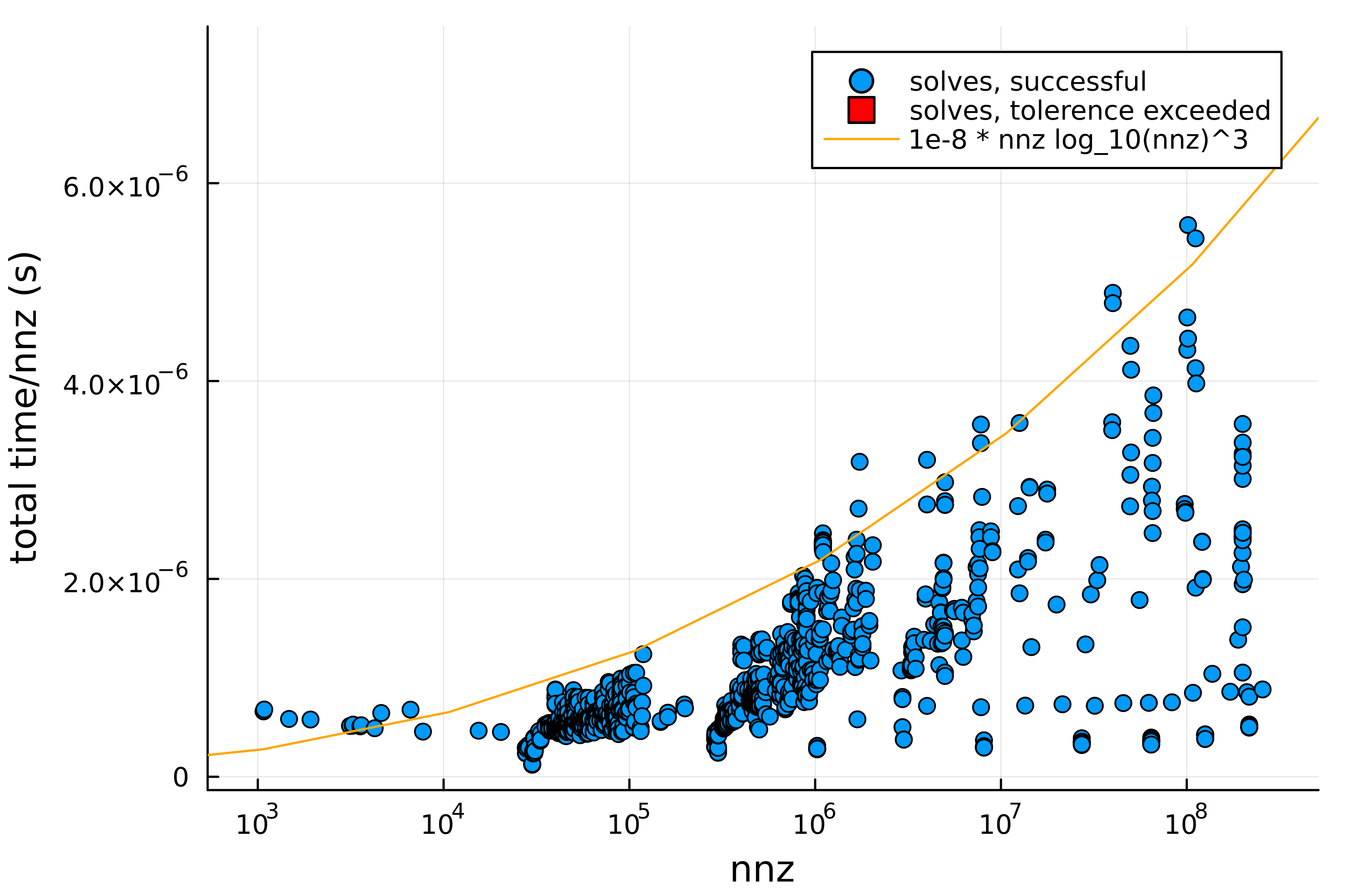
Figure 6: The plot shows data from all our experiments with the AC2 with total running time per non-zero in seconds on the y-axis plotted against the number-of-non-zeros of the instance on the x-axis. Solves are shown with a blue circle. All solves reached the target tolerance. An orange line shows the function $\operatorname{nnz}\log_{10}(\operatorname{nnz})^{3}$ (seconds) where $\operatorname{nnz}$ is the non-zero count, and the same normalization is used as for the data (i.e. dividing by $\operatorname{nnz}$).

Appendix A Linear Algebra and Cholesky Background

We introduce some basic notation and definitions from linear algebra.

Moore-Penrose pseudo-inverse.

We use $\bm{\mathit{B}}^{\dagger}$ to denote the Moore-Penrose pseudo-inverse of a matrix $\bm{\mathit{B}}$. Let $\bm{1}\in\mathbb{R}^{n}$ denote the all ones vector, with dimension $n$ that will always be made clear in the context of its use. Similarly, we let $\bm{0}$ denote the all zero vector or matrix, depending on context.

The following fact is useful, since we often need to apply the pseodo-inverse of a matrix.

Fact A.1 (Pseudo-inverse of a product).

Suppose $\bm{\mathit{M}}=\bm{\mathit{A}}\bm{\mathit{B}}\bm{\mathit{C}}$ is square real matrix, where $\bm{\mathit{A}}$ and $\bm{\mathit{C}}$ are non-singular. Then

$$\bm{\mathit{M}}^{\dagger}=\bm{\Pi}_{\bm{\mathit{M}}}\bm{\mathit{C}}^{-1}\bm{\mathit{B}}^{\dagger}\bm{\mathit{A}}^{-1}\bm{\Pi}_{\bm{\mathit{M}}^{\top}}.$$

LU-decomposition and Cholesky factorization of singular matrices.

An LU-decomposition of a square matrix $\bm{\mathit{M}}\in\mathbb{R}^{n\times n}$ is a factorization $\bm{\mathit{M}}=\bm{\mathit{{\mathcal{L}}}}\bm{\mathit{{\mathcal{U}}}}$, where $\bm{\mathit{{\mathcal{L}}}}$ is a lower-triangular matrix and $\bm{\mathit{{\mathcal{U}}}}$ is an upper-triangular matrix, both up to a permutation.

When the matrix $\bm{\mathit{M}}$ is symmetrix and positive semi-definite, study a special case of LU-decomposition, where $\bm{\mathit{{\mathcal{U}}}}=\bm{\mathit{{\mathcal{L}}}}^{\top}$, i.e. $\bm{\mathit{M}}=\bm{\mathit{{\mathcal{L}}}}\bm{\mathit{{\mathcal{L}}}}^{\top}$. This is known as a Cholesky Factorization.

When $\bm{\mathit{M}}$ is non-singular, the linear equations $\bm{\mathit{{\mathcal{L}}}}\bm{\mathit{y}}=\bm{\mathit{b}}$ and $\bm{\mathit{{\mathcal{U}}}}\bm{\mathit{x}}=\bm{\mathit{y}}$ and be solved by forward and backward substitution algorithms respectively (e.g. see [TBI97]), which run in time $O(\operatorname{nnz}(\bm{\mathit{{\mathcal{L}}}}))$ and $O(\operatorname{nnz}(\bm{\mathit{{\mathcal{U}}}}))$. I.e. $\bm{\mathit{{\mathcal{L}}}}^{-1}$ and $\bm{\mathit{{\mathcal{U}}}}^{-1}$ can be applied in time proportional to the number of non-zeros in $\bm{\mathit{{\mathcal{L}}}}$ and $\bm{\mathit{{\mathcal{U}}}}$ respectively. This means that if a decomposition $\bm{\mathit{{\mathcal{L}}}},\bm{\mathit{{\mathcal{U}}}}$ of $\bm{\mathit{M}}$ is known, then linear systems in $\bm{\mathit{M}}$ be solved in time $O(\operatorname{nnz}(\bm{\mathit{{\mathcal{L}}}})+\operatorname{nnz}(\bm{\mathit{{\mathcal{U}}}}))$, since $\bm{\mathit{M}}\bm{\mathit{x}}=\bm{\mathit{b}}$ implies $\bm{\mathit{x}}=\bm{\mathit{{\mathcal{U}}}}^{-1}\bm{\mathit{{\mathcal{L}}}}^{-1}\bm{\mathit{b}}$.

When $\bm{\mathit{M}}$ is singular the same forward and backward substitution algorithms can be used to compute the pseudo-inverse, in some situations. We focus on a special case where we can instead factor $\bm{\mathit{M}}$ as $\bm{\mathit{M}}=\bm{\mathit{{\mathcal{L}}}}^{\prime}\bm{\mathit{{\mathcal{D}}}}\bm{\mathit{{\mathcal{U}}}}^{\prime}$, where $\bm{\mathit{{\mathcal{D}}}}$ is singular and $\bm{\mathit{{\mathcal{L}}}}^{\prime}$, $\bm{\mathit{{\mathcal{U}}}}^{\prime}$ are non-singular.

For the case of interest to us, Laplacians of connected graphs, this slightly modified factorization can be trivially obtained from an LU-decomposition, by $\bm{\mathit{{\mathcal{L}}}}^{\prime}$ equal to $\bm{\mathit{{\mathcal{L}}}}$ except $\bm{\mathit{{\mathcal{L}}}}(n,n)=1$ and $\bm{\mathit{{\mathcal{U}}}}^{\prime}$ equal to $\bm{\mathit{{\mathcal{U}}}}$ except $\bm{\mathit{{\mathcal{U}}}}(n,n)=1$ and taking $\bm{\mathit{{\mathcal{D}}}}$ to be the identity matrix, except $\bm{\mathit{{\mathcal{D}}}}(n,n)=0$. For our approximate factorizations of Laplacians, the matrix $\bm{\mathit{M}}=\bm{\mathit{{\mathcal{L}}}}^{\prime}\bm{\mathit{{\mathcal{D}}}}\bm{\mathit{{\mathcal{U}}}}^{\prime}$ is symmetric with $\bm{\mathit{{\mathcal{U}}}}^{\prime}=(\bm{\mathit{{\mathcal{L}}}}^{\prime})^{\top}$, hence $\bm{\Pi}_{\bm{\mathit{M}}^{\top}}=\bm{\Pi}_{\bm{\mathit{M}}}$. Now, by Fact A.1,

$$\bm{\mathit{M}}^{\dagger}=\bm{\Pi}_{\bm{\mathit{M}}}(\bm{\mathit{{\mathcal{L}}}}^{\prime})^{-\top}\bm{\mathit{{\mathcal{D}}}}^{\dagger}\bm{\mathit{{\mathcal{L}}}}^{-1}\bm{\Pi}_{\bm{\mathit{M}}}.$$ (29)

The kernel of $\bm{\mathit{M}}$ is precisely the span of the indicator vectors of each connected component of the associated graph, and hence $\bm{\Pi}_{\bm{\mathit{M}}}$ can be applied by, for each connected component, subtracting the mean value for that component from every entry of the component.

Appendix B Unbiased approximate Cholesky factorization

In this section, for completeness, we prove Claim 4.1, which was shown in [KS16].

Claim B.1.

When ApproximateCholesky is instantiated with an unbiased clique sampling routine CliqueSample so that

$$\mathop{{}\mathbb{E}}\left[\textsc{CliqueSample}(v,\SS)\right]=\textsc{Clique}\!\left[{\SS}\right]_{v}.$$

Then letting $\bm{\mathit{{\mathcal{L}}}}=\textsc{ApproximateCholesky}(\bm{\mathit{L}})$, we have

$$\mathop{{}\mathbb{E}}\left[\bm{\mathit{{\mathcal{L}}}}\bm{\mathit{{\mathcal{L}}}}^{\top}\right]=\bm{\mathit{L}}.$$

In other words, the approximate Cholesky factorization equals the original matrix in expectation, which is in turn also equal, viewed as a linear operator, to any exact Cholesky factorization.

Proof.

Let $\SS_{i}$ denote $\SS$ in Algorithm 2 after $i$ eliminations, and note that $\SS_{0}=\bm{\mathit{L}}$. Let

$$\bm{\mathit{L}}_{i}=\SS_{i}+\sum_{j=1}^{i}\bm{\mathit{l}}_{j}\bm{\mathit{l}}_{j}^{\top}.$$

Suppose the $i$th vertex to be eliminated is vertex $v$. Conditional on the samples before the $i$th elimination, we have

$$\mathop{{}\mathbb{E}}\left[\bm{\mathit{L}}_{i}\right] =\mathop{{}\mathbb{E}}\left[\SS_{i}+\sum_{j=1}^{i}\bm{\mathit{l}}_{j}\bm{\mathit{l}}_{j}^{\top}\right].$$

$$=\mathop{{}\mathbb{E}}\left[\SS_{i-1}-\textsc{Star}\!\left[\SS_{i-1}\right]_{v}+\textsc{CliqueSample}(v,\SS_{i-1})+\sum_{j=1}^{i}\bm{\mathit{l}}_{j}\bm{\mathit{l}}_{j}^{\top}\right]$$

$$=\SS_{i-1}-\textsc{Star}\!\left[\SS_{i-1}\right]_{v}+\mathop{{}\mathbb{E}}\left[\textsc{CliqueSample}(v,\SS_{i-1})\right]+\sum_{j=1}^{i}\bm{\mathit{l}}_{j}\bm{\mathit{l}}_{j}^{\top}$$

$$=\SS_{i-1}-\textsc{Star}\!\left[\SS_{i-1}\right]_{v}+\textsc{Clique}\!\left[{\SS_{i-1}}\right]_{v}+\sum_{j=1}^{i}\bm{\mathit{l}}_{j}\bm{\mathit{l}}_{j}^{\top}$$

$$=\SS_{i-1}+\sum_{j=1}^{i-1}\bm{\mathit{l}}_{j}\bm{\mathit{l}}_{j}^{\top}$$

$$=\bm{\mathit{L}}_{i-1}.$$

We can now chain together expectations to conclude that over all the randomness of the algorithm

$$\mathop{{}\mathbb{E}}\left[\bm{\mathit{{\mathcal{L}}}}\bm{\mathit{{\mathcal{L}}}}^{\top}\right]=\mathop{{}\mathbb{E}}\left[\bm{\mathit{L}}_{n}\right]=\bm{\mathit{L}}.$$

∎

Appendix C Equivalence of the output representations

In this section, we prove Claim 4.8, about the equivalence of edgewise and standard Cholesky factorization. We restate the lemma here for convenience:

Claim.

Suppose we run both ApproximateCholesky and ApproximateEdgewiseCholesky

• using the same elimination ordering,

• and using CliqueTreeSample as the clique sampling routine, and using the same outputs of CliqueTreeSample, i.e. the same outcomes of the random samples.

Then the output factorizations $\bm{\mathit{{\mathcal{L}}}}$ from ApproximateCholesky and $\bm{\Phi},\left\{\bm{\mathit{{\mathcal{L}}}}^{(v)}_{i}\right\}_{v,i}$ from ApproximateEdgewiseCholesky will satisfy

$$\bm{\mathit{{\mathcal{L}}}}\bm{\mathit{{\mathcal{L}}}}^{\top}=\left(\Pi_{i=1}^{n}\Pi_{j\sim i}\bm{\mathit{{\mathcal{L}}}}_{j}^{(i)}\right)\bm{\Phi}\left(\Pi_{i=1}^{n}\Pi_{j\sim i}\bm{\mathit{{\mathcal{L}}}}_{j}^{(i)}\right)^{\top}.$$

In other words, the only difference between the two algorithms is in the formatting of the output.

Proof.

We can write a Laplacian $\bm{\mathit{L}}$ with terms corresponding to edges of the first vertex explicitly separated out as:

$$\bm{\mathit{L}}=\left(\begin{array}[]{ccc}d&-\boldsymbol{\mathit{a}}^{\top}\\ -\boldsymbol{\mathit{a}}&\operatorname*{diag}(\boldsymbol{\mathit{a}})+\bm{\mathit{L}}_{-1}\end{array}\right)$$ (30)

Here $\bm{\mathit{L}}_{-1}$ is the graph Laplacian corresponding to the induced subgraph on the vertex set with vertex 1 removed.

From Section 4.1, we know that it is possible to write

$$\bm{\mathit{L}}=\begin{pmatrix}0&\bm{0}^{\top}\\ \bm{0}&\SS\end{pmatrix}+\frac{1}{d}\begin{pmatrix}d\\ -\boldsymbol{\mathit{a}}\end{pmatrix}\begin{pmatrix}d\\ -\boldsymbol{\mathit{a}}\end{pmatrix}^{\top}$$ (31)

where $\SS=\textsc{Sc}\!\left[\bm{\mathit{L}}\right]_{[n]\setminus\left\{1\right\}}$.

If vertex $1$ has $k$ neighbors, then using the elimination procedure described in Section 4.4 to eliminate the first row and column of the matrix will result in a partial factorization. Thus,

$$\bm{\mathit{L}}=\bm{\mathit{{\mathcal{L}}}}_{1}\bm{\mathit{{\mathcal{L}}}}_{2}\ldots\bm{\mathit{{\mathcal{L}}}}_{k}\left(\begin{array}[]{ccc}\phi&\bm{0}^{\top}\\ \bm{0}&\SS\end{array}\right)\bm{\mathit{{\mathcal{L}}}}_{k}^{\top}\ldots\bm{\mathit{{\mathcal{L}}}}_{2}^{\top}\bm{\mathit{{\mathcal{L}}}}_{1}^{\top}$$ (32)

where each $\bm{\mathit{{\mathcal{L}}}}_{i}^{\top}$ is a lower-triangular matrix corresponding to a single row-operation.

We can prove the following:

$$\left(\begin{array}[]{ccc}0&\bm{0}^{\top}\\ \bm{0}&\SS\end{array}\right)=\bm{\mathit{{\mathcal{L}}}}_{1}\bm{\mathit{{\mathcal{L}}}}_{2}\cdots\bm{\mathit{{\mathcal{L}}}}_{k}\left(\begin{array}[]{ccc}0&\bm{0}^{\top}\\ \bm{0}&\SS\end{array}\right)\bm{\mathit{{\mathcal{L}}}}_{k}^{\top}\cdots\bm{\mathit{{\mathcal{L}}}}_{2}^{\top}\bm{\mathit{{\mathcal{L}}}}_{1}^{\top}$$ (33)

and

$$\frac{1}{d}\begin{pmatrix}d\\ -\boldsymbol{\mathit{a}}\end{pmatrix}\begin{pmatrix}d\\ -\boldsymbol{\mathit{a}}\end{pmatrix}^{\top}=\bm{\mathit{{\mathcal{L}}}}_{1}\bm{\mathit{{\mathcal{L}}}}_{2}\cdots\bm{\mathit{{\mathcal{L}}}}_{k}\left(\begin{array}[]{ccc}\phi&\bm{0}^{\top}\\ \bm{0}&\bm{0}\end{array}\right)\bm{\mathit{{\mathcal{L}}}}_{k}^{\top}\cdots\bm{\mathit{{\mathcal{L}}}}_{2}^{\top}\bm{\mathit{{\mathcal{L}}}}_{1}^{\top}$$ (34)

To establish Equation (33), we observe that each row operation factor takes the form

$$\bm{\mathit{{\mathcal{L}}}}_{i}=\begin{pmatrix}\bm{\mathit{b}}_{i}&\bm{0}^{\top}\\ \vrule&\bm{\mathit{I}}_{(n-1)\times(n-1)}\end{pmatrix}$$

for some vector $\bm{\mathit{b}}_{i}\in R^{n}$. But, given any vector $\bm{\mathit{b}}_{i}\in R^{n}$ and any matrix $\bm{\mathit{C}}\in R^{(n-1)\times d}$, with any number of columns $d$, we have

$$\begin{pmatrix}\bm{\mathit{b}}&\bm{0}^{\top}\\ \vrule&\bm{\mathit{I}}_{(n-1)\times(n-1)}\end{pmatrix}\begin{pmatrix}\bm{0}^{\top}\\ \bm{\mathit{C}}\end{pmatrix}=\begin{pmatrix}\bm{0}^{\top}\\ \bm{\mathit{C}}\end{pmatrix}.$$

Repeatedly applying this observation the right hand side of Equation (33) lets us conclude that it equals the left hand side, proving the equation holds.

Now, by equating the two right hand sides of Equation (31) and Equation (24), and simplifying using Equation (33), we conclude that Equation (34) holds.

The proof of Equation (34) only relies on the row operation matrices having the form $\bm{\mathit{{\mathcal{L}}}}_{i}=\begin{pmatrix}\bm{\mathit{b}}_{i}&\bm{0}^{\top}\\ \vrule&\bm{\mathit{I}}_{(n-1)\times(n-1)}\end{pmatrix}$ for some $\bm{\mathit{b}}_{i}$ and does not require $\SS$ to be a Schur complement.

Consquently, it holds for any $\bm{\mathit{\tilde{S}}}$ matrix that

$$\left(\begin{array}[]{ccc}0&\bm{0}^{\top}\\ \bm{0}&\bm{\mathit{\tilde{S}}}\end{array}\right)=\bm{\mathit{{\mathcal{L}}}}_{1}\bm{\mathit{{\mathcal{L}}}}_{2}\cdots\bm{\mathit{{\mathcal{L}}}}_{k}\left(\begin{array}[]{ccc}0&\bm{0}^{\top}\\ \bm{0}&\bm{\mathit{\tilde{S}}}\end{array}\right)\bm{\mathit{{\mathcal{L}}}}_{k}^{\top}\cdots\bm{\mathit{{\mathcal{L}}}}_{2}^{\top}\bm{\mathit{{\mathcal{L}}}}_{1}^{\top}$$ (35)

and hence

$$\begin{pmatrix}0&\bm{0}^{\top}\\ \bm{0}&\bm{\mathit{\tilde{S}}}\end{pmatrix}+\frac{1}{d}\begin{pmatrix}d\\ -\boldsymbol{\mathit{a}}\end{pmatrix}\begin{pmatrix}d\\ -\boldsymbol{\mathit{a}}\end{pmatrix}^{\top}=\bm{\mathit{{\mathcal{L}}}}_{1}\bm{\mathit{{\mathcal{L}}}}_{2}\cdots\bm{\mathit{{\mathcal{L}}}}_{k}\left(\begin{array}[]{ccc}\phi&\bm{0}^{\top}\\ \bm{0}&\bm{\mathit{\tilde{S}}}\end{array}\right)\bm{\mathit{{\mathcal{L}}}}_{k}^{\top}\cdots\bm{\mathit{{\mathcal{L}}}}_{2}^{\top}\bm{\mathit{{\mathcal{L}}}}_{1}^{\top}.$$ (36)

Thus, by taking $\bm{\mathit{\tilde{S}}}=\bm{\mathit{L}}_{-1}+\textsc{CliqueTreeSample}(v,\SS)$, we can conclude that the partial factorizations computed in one step of $\textsc{ApproximateCholesky}(\bm{\mathit{L}})$ and $\textsc{EdgewiseApproximateCholesky}(\bm{\mathit{L}})$ are identical. We can apply this equivalence repeatedly to conclude that the two approximate factorizations returned by $\textsc{ApproximateCholesky}(\bm{\mathit{L}})$ and $\textsc{EdgewiseApproximateCholesky}(\bm{\mathit{L}})$ are identical, assuming we

• use the same elimination ordering for both,

• and use CliqueTreeSample as the clique sampling routine, and using the same outputs of CliqueTreeSample, i.e. the same outcomes of the random samples.

Thus the approximate factorizations returned by $\textsc{ApproximateCholesky}(\bm{\mathit{L}})$ and EdgewiseApproximateCholesky(L) are identical when regarded as operators.

∎

References

- [ADD96] Patrick R Amestoy, Timothy A Davis, and Iain S Duff. An approximate minimum degree ordering algorithm. SIAM Journal on Matrix Analysis and Applications, 17(4):886–905, 1996.
- [BAA+19] Satish Balay, Shrirang Abhyankar, Mark Adams, Jed Brown, Peter Brune, Kris Buschelman, Lisandro Dalcin, Alp Dener, Victor Eijkhout, and W. Gropp. PETSc users manual. 2019.
- [BBC+94] Richard Barrett, Michael Berry, Tony F. Chan, James Demmel, June Donato, Jack Dongarra, Victor Eijkhout, Roldan Pozo, Charles Romine, and Henk Van der Vorst. Templates for the Solution of Linear Systems: Building Blocks for Iterative Methods. SIAM, 1994.
- [BCHT04] Erik G. Boman, Doron Chen, Bruce Hendrickson, and Sivan Toledo. Maximum-weight-basis preconditioners. Numerical Linear Algebra with Applications, 11(8-9):695–721, 2004.
- [BCK+18] James Brannick, Fei Cao, Karsten Kahl, Robert D. Falgout, and Xiaozhe Hu. Optimal interpolation and compatible relaxation in classical algebraic multigrid. SIAM Journal on Scientific Computing, 40(3):A1473–A1493, 2018.
- [BD79] Achi Brandt and Nathan Dinar. Multigrid Solutions to Elliptic Flow Problems. In SEYMOUR V. Parter, editor, Numerical Methods for Partial Differential Equations, pages 53–147. Academic Press, January 1979.
- [BDG16] Erik G. Boman, Kevin Deweese, and John R. Gilbert. Evaluating the Dual Randomized Kaczmarz Laplacian Linear Solver. Informatica, 40(1):95–107, March 2016.
- [Bea94] Robert Beauwens. Approximate factorizations with modified s/p consistently ordered m-factors. Numerical linear algebra with applications, 1(1):3–17, 1994.
- [BGH+06a] Marshall Bern, John R. Gilbert, Bruce Hendrickson, Nhat Nguyen, and Sivan Toledo. Support-graph preconditioners. SIAM Journal on Matrix Analysis and Applications, 27(4):930–951, 2006.
- [BGH+06b] Marshall Bern, John R. Gilbert, Bruce Hendrickson, Nhat Nguyen, and Sivan Toledo. Support-graph preconditioners. SIAM Journal on Matrix Analysis and Applications, 27(4):930–951, 2006.
- [BGH+19] Luc Berger-Vergiat, Christian Alexander Glusa, Jonathan J. Hu, Christopher Siefert, Raymond S. Tuminaro, Mayr Matthias, Prokopenko Andrey, and Wiesner Tobias. MueLu User’s Guide. Technical report, Sandia National Lab.(SNL-NM), Albuquerque, NM (United States); Sandia …, 2019.
- [BH83] Dietrich Braess and Wolfgang Hackbusch. A new convergence proof for the multigrid method including the V-cycle. SIAM journal on numerical analysis, 20(5):967–975, 1983.
- [BH03] Erik G. Boman and Bruce Hendrickson. Support Theory for Preconditioning. SIAM Journal on Matrix Analysis and Applications, 25(3):694–717, January 2003.
- [BHV08] Erik G. Boman, Bruce Hendrickson, and Stephen Vavasis. Solving Elliptic Finite Element Systems in Near-Linear Time with Support Preconditioners. SIAM Journal on Numerical Analysis, 46(6):3264–3284, January 2008.
- [Bra77] Achi Brandt. Multi-level adaptive solutions to boundary-value problems. Mathematics of computation, 31(138):333–390, 1977.
- [Bra00] Achi Brandt. General highly accurate algebraic coarsening. Electronic Transactions on Numerical Analysis, 10(1):21, 2000.
- [Bra02] Achi Brandt. Multiscale scientific computation: Review 2001. Multiscale and multiresolution methods, pages 3–95, 2002.
- [CB01] M. A. Christie and M. J. Blunt. Tenth SPE Comparative Solution Project: A Comparison of Upscaling Techniques. In SPE Reservoir Simulation Symposium. OnePetro, February 2001.
- [CCB+20] Léopold Cambier, Chao Chen, Erik G. Boman, Sivasankaran Rajamanickam, Raymond S. Tuminaro, and Eric Darve. An Algebraic Sparsified Nested Dissection Algorithm Using Low-Rank Approximations. arXiv:1901.02971 [cs, math], January 2020.
- [CKP+14] Michael B. Cohen, Rasmus Kyng, Jakub W. Pachocki, Richard Peng, and Anup Rao. Preconditioning in expectation. arXiv preprint arXiv:1401.6236, 2014.
- [CLB21] Chao Chen, Tianyu Liang, and George Biros. RCHOL: Randomized Cholesky factorization for solving SDD linear systems. SIAM Journal on Scientific Computing, 43(6):C411–C438, 2021.
- [CT03] Doron Chen and Sivan Toledo. Vaidya’s preconditioners: Implementation and experimental study. Electronic Transactions on Numerical Analysis, 16(9):03, 2003.
- [DGM+16] Kevin Deweese, John R. Gilbert, Gary Miller, Richard Peng, Hao Ran Xu, and Shen Chen Xu. An empirical study of cycle toggling based Laplacian solvers. In 2016 Proceedings of the Seventh SIAM Workshop on Combinatorial Scientific Computing, pages 33–41. SIAM, 2016.
- [DH11] Timothy A. Davis and Yifan Hu. The university of Florida sparse matrix collection. ACM Transactions on Mathematical Software, 38(1):1:1–1:25, December 2011.
- [FY02] Robert D. Falgout and Ulrike Meier Yang. Hypre: A library of high performance preconditioners. In International Conference on Computational Science, pages 632–641. Springer, 2002.
- [Gre96] Keith D. Gremban. Combinatorial Preconditioners for Sparse, Symmetric, Diagonally Dominant Linear Systems. PhD Thesis, Carnegie Mellon University, 1996.
- [GRV09] Navin Goyal, Luis Rademacher, and Santosh Vempala. Expanders via random spanning trees. In Proceedings of the Twentieth Annual ACM-SIAM Symposium on Discrete Algorithms, pages 576–585. SIAM, 2009.
- [Gus78] Ivar Gustafsson. A class of first order factorization methods. BIT Numerical Mathematics, 18(2):142–156, 1978.
- [GVL13] Gene H. Golub and Charles F. Van Loan. Matrix Computations. Johns Hopkins Studies in the Mathematical Sciences. The Johns Hopkins University Press, Baltimore, fourth edition edition, 2013.
- [HJPW23] Monika Henzinger, Billy Jin, Richard Peng, and David P. Williamson. A Combinatorial Cut-Toggling Algorithm for Solving Laplacian Linear Systems. In Yael Tauman Kalai, editor, 14th Innovations in Theoretical Computer Science Conference (ITCS 2023), volume 251 of Leibniz International Proceedings in Informatics (LIPIcs), pages 69:1–69:22, Dagstuhl, Germany, 2023. Schloss Dagstuhl – Leibniz-Zentrum für Informatik.
- [HLMW16] Daniel Hoske, Dimitar Lukarski, Henning Meyerhenke, and Michael Wegner. Engineering a combinatorial Laplacian solver: Lessons learned. Algorithms, 9(4):72, 2016.
- [HY02] Van Emden Henson and Ulrike Meier Yang. BoomerAMG: A parallel algebraic multigrid solver and preconditioner. Applied Numerical Mathematics, 41(1):155–177, April 2002.
- [JS21] Arun Jambulapati and Aaron Sidford. Ultrasparse Ultrasparsifiers and Faster Laplacian System Solvers. In Proceedings of the 2021 ACM-SIAM Symposium on Discrete Algorithms (SODA), pages 540–559. SIAM, 2021.
- [Ker78] David S Kershaw. The incomplete Cholesky—conjugate gradient method for the iterative solution of systems of linear equations. Journal of Computational Physics, 26(1):43–65, January 1978.
- [KKS22] Tali Kaufman, Rasmus Kyng, and Federico Soldá. Scalar and Matrix Chernoff Bounds from $\ell_{\infty}$-Independence. SODA ’22: Proceedings of the Thirty-Third Annual ACM-SIAM Symposium on Discrete Algorithms, January 2022.
- [KLP+16] Rasmus Kyng, Yin Tat Lee, Richard Peng, Sushant Sachdeva, and Daniel A. Spielman. Sparsified cholesky and multigrid solvers for connection laplacians. In Proceedings of the Forty-Eighth Annual ACM Symposium on Theory of Computing, pages 842–850, 2016.
- [KLS20] Tarun Kathuria, Yang P. Liu, and Aaron Sidford. Unit Capacity Maxflow in Almost $ O (m$̂{$4/3$}$) $ Time. In 2020 IEEE 61st Annual Symposium on Foundations of Computer Science (FOCS), pages 119–130. IEEE, 2020.
- [KMP10] Ioannis Koutis, Gary L. Miller, and Richard Peng. Approaching Optimality for Solving SDD Linear Systems. In Proceedings of the 2010 IEEE 51st Annual Symposium on Foundations of Computer Science, FOCS ’10, pages 235–244, USA, October 2010. IEEE Computer Society.
- [KMP11] Ioannis Koutis, Gary L. Miller, and Richard Peng. A nearly-m log n time solver for sdd linear systems. In 2011 IEEE 52nd Annual Symposium on Foundations of Computer Science, pages 590–598. IEEE, 2011.
- [KMT11] Ioannis Koutis, Gary L. Miller, and David Tolliver. Combinatorial preconditioners and multilevel solvers for problems in computer vision and image processing. Computer Vision and Image Understanding, 115(12):1638–1646, December 2011.
- [KOSZ13] Jonathan A. Kelner, Lorenzo Orecchia, Aaron Sidford, and Zeyuan Allen Zhu. A simple, combinatorial algorithm for solving SDD systems in nearly-linear time. In Proceedings of the Forty-Fifth Annual ACM Symposium on Theory of Computing, pages 911–920, 2013.
- [KS16] Rasmus Kyng and Sushant Sachdeva. Approximate gaussian elimination for laplacians-fast, sparse, and simple. In 2016 IEEE 57th Annual Symposium on Foundations of Computer Science (FOCS), pages 573–582. IEEE, 2016.
- [KS18] Rasmus Kyng and Zhao Song. A matrix chernoff bound for strongly rayleigh distributions and spectral sparsifiers from a few random spanning trees. In 2018 IEEE 59th Annual Symposium on Foundations of Computer Science (FOCS), pages 373–384. IEEE, 2018.
- [LB12] Oren E. Livne and Achi Brandt. Lean algebraic multigrid (LAMG): Fast graph Laplacian linear solver. SIAM Journal on Scientific Computing, 34(4):B499–B522, 2012.
- [LHL+19] M. Harper Langston, Mitchell Tong Harris, Pierre-David Letourneau, Richard Lethin, and James Ezick. Combinatorial Multigrid: Advanced Preconditioners For Ill-Conditioned Linear Systems. In 2019 IEEE High Performance Extreme Computing Conference (HPEC), pages 1–7, Waltham, MA, USA, September 2019. IEEE.
- [Mv77] J. A. Meijerink and H. A. van der Vorst. An Iterative Solution Method for Linear Systems of Which the Coefficient Matrix is a Symmetric $M$-Matrix. Mathematics of Computation, 31(137):148–162, 1977.
- [NN17] Artem Napov and Yvan Notay. An Efficient Multigrid Method for Graph Laplacian Systems II: Robust Aggregation. SIAM Journal on Scientific Computing, 39(5):S379–S403, January 2017.
- [Not90] Yvan Notay. Solving positive (semi) definite linear systems by preconditioned iterative methods. In Preconditioned Conjugate Gradient Methods, pages 105–125. Springer, 1990.
- [Not92] Yvan Notay. Conditioning of stieltjes matrices by s/p consistently ordered approximate factorizations. Applied numerical mathematics, 10(5):381–396, 1992.
- [PS14] Richard Peng and Daniel A. Spielman. An efficient parallel solver for SDD linear systems. In Proceedings of the Forty-Sixth Annual ACM Symposium on Theory of Computing, pages 333–342, 2014.
- [RS87] John W. Ruge and Klaus Stüben. Algebraic multigrid. In Multigrid Methods, pages 73–130. SIAM, 1987.
- [SBB+12] H. Sundar, G. Biros, C. Burstedde, J. Rudi, O. Ghattas, and G. Stadler. Parallel geometric-algebraic multigrid on unstructured forests of octrees. In SC ’12: Proceedings of the International Conference on High Performance Computing, Networking, Storage and Analysis, pages 1–11, November 2012.
- [ST04] Daniel A. Spielman and Shang-Hua Teng. Nearly-linear time algorithms for graph partitioning, graph sparsification, and solving linear systems. In Proceedings of the Thirty-Sixth Annual ACM Symposium on Theory of Computing, STOC ’04, pages 81–90, New York, NY, USA, June 2004. Association for Computing Machinery.
- [TBI97] Lloyd N. Trefethen and David Bau III. Numerical Linear Algebra, volume 50. Siam, 1997.
- [Vai90] Pravin M. Vaidya. Solving linear equations with symmetric diagonally dominant matrices by constructing good preconditioners. 1990.
- [vM77] HA van der Vorst, and JA Meijerink. An iterative solution method for linear systems of which the coefficient matrix is a symmetric M-matrix. Math. Comput, 31:148, 1977.
- [Yse93] Harry Yserentant. Old and new convergence proofs for multigrid methods. Acta numerica, 2:285–326, 1993.
- [ZGL03] Xiaojin Zhu, Zoubin Ghahramani, and John D. Lafferty. Semi-supervised learning using gaussian fields and harmonic functions. In Proceedings of the 20th International Conference on Machine Learning (ICML-03), pages 912–919, 2003.