The Virtues of Laziness in Model-based RL: A Unified Objective and Algorithms

Abstract

We propose a novel approach to addressing two fundamental challenges in Model-based Reinforcement Learning (MBRL): the computational expense of repeatedly finding a good policy in the learned model, and the objective mismatch between model fitting and policy computation. Our “lazy” method leverages a novel unified objective, Performance Difference via Advantage in Model, to capture the performance difference between the learned policy and expert policy under the true dynamics. This objective demonstrates that optimizing the expected policy advantage in the learned model under an exploration distribution is sufficient for policy computation, resulting in a significant boost in computational efficiency compared to traditional planning methods. Additionally, the unified objective uses a value moment matching term for model fitting, which is aligned with the model’s usage during policy computation. We present two no-regret algorithms to optimize the proposed objective, and demonstrate their statistical and computational gains compared to existing MBRL methods through simulated benchmarks.

1 Introduction

Model-based Reinforcement Learning (MBRL) methods show great promise for real world applicability as they often require remarkably fewer number of real world interactions compared to model-free counterparts (Schrittwieser et al., 2020; Hafner et al., 2023). The key idea is that, in contrast to model-free RL that computes a policy directly from real world data, we can perform the following iterative procedure (Sutton & Barto, 2018): we fit a model that accurately predicts the dynamics on the data collected so far using the learned policy. Subsequently, we compute a policy through optimal planning in the learned model, and use it to collect more data in the real world. This procedure is repeated until a satisfactory policy is learned. Theoretical studies, such as Ross & Bagnell (2012), have shown that this procedure can find a near-optimal policy in a statistically efficient manner under certain conditions, such as access to a good exploration distribution and a rich enough model class, and this has been validated by its good performance in practice.

However, there are two major challenges with the above procedure. The policy computation step in each iteration relies on solving the computationally expensive problem of finding the best policy in the learned model. This can require a number of interactions in the model that is exponential in the task horizon (Kearns et al., 1999). Furthermore, past literature including Ross & Bagnell (2012); Jiang (2018); Vemula et al. (2020) among others have shown that optimal planning in learned models can result in policies that exploit inaccuracies in the learned model hindering fast learning and statistical efficiency.

The second challenge pertains to the objective mismatch between model fitting and policy computation that is extensively studied in recent literature (Farahmand et al., 2017; Lambert et al., 2020). The model fitting objective of minimizing prediction error is not necessarily related to the objective of maximizing the performance of the policy, derived from the model, in the real world. This results in a mismatch of objectives used to fit the model and how the model is used when computing the policy through planning. This is exacerbated in cases where the model class is not realizable, i.e. no model in the model class can perfectly explain true dynamics, which is often the case in real world tasks (Joseph et al., 2013).

In this work, we propose a new decomposition of the performance difference between the learned policy and expert policy under true dynamics, which we coin as Performance Difference via Advantage in Model. This leads to a unified objective that informs two major changes to the existing MBRL procedure. Instead of computing the optimal policy in the learned model at each iteration, we optimize the expected policy advantage in the model under an exploration distribution which only requires a number of interactions in the model that is polynomial in the task horizon. For model fitting, our new objective measures the similarity of predicted and observed next states in terms of their value function in the learned model. This ensures that the model is updated to be accurate in states that are critical for policy computation, and allows for inaccuracy in states that are irrelevant. Therefore, our proposed unified objective encourages “laziness” in both steps of the MBRL procedure, solving both the computational expense and objective mismatch challenges.

Our contributions in this paper are as follows:

• A unified objective for MBRL that is both computationally more efficient in policy computation and resolves the objective mismatch in model fitting.

• Two algorithms that leverage the laziness in the proposed objective to achieve tighter performance bounds than those of Ross & Bagnell (2012).

• An empirical demonstration through simulated benchmarks that our proposed algorithms result in both statistical and computational gains compared to existing MBRL methods.

2 Related Work

Model-based RL Model-based Reinforcement Learning and Optimal Control have been extensively researched in the literature, with a long line of works (Ljung, 1998; Morari & Lee, 1999; Sutton, 1991). Recent work has made significant achievements in tasks with both low-dimensional state spaces (Levine & Abbeel, 2014; Chua et al., 2018; Schrittwieser et al., 2020) and high-dimensional state spaces (Hafner et al., 2020; Wu et al., 2022). Theoretical studies have also been conducted to analyze the performance guarantees and sample complexity of model-based methods (Abbasi-Yadkori & Szepesvári, 2011; Ross & Bagnell, 2012; Tu & Recht, 2019; Sun et al., 2019a). However, there is a common requirement among previous works to compute the optimal policy from the learned model at each iteration, using methods that range from value iteration (Azar et al., 2013) to black-box policy optimization (Kakade et al., 2020; Song & Sun, 2021). In this work, we show that computing the optimal policy in the learned model is not necessary and propose a computationally efficient alternative that does not compromise performance guarantees.

RL with exploration distribution In this work, as well as in previous works such as Kakade & Langford (2002); Bagnell et al. (2003); Ross & Bagnell (2014), we assume access to an exploration distribution that allows us to exploit any prior knowledge of the task to learn good policies quickly. We also leverage a similar model-free policy search algorithm in this work within the MBRL framework. Recent works in the field of Hybrid Reinforcement Learning (Rajeswaran et al., 2017; Vecerik et al., 2017; Nair et al., 2018; Hester et al., 2018; Xie et al., 2021b; Song et al., 2022) consider a related setting where both an offline dataset and online access to interact with environment are available. However, most of these works are in the model-free setting and require that the offline dataset is collected from an expert policy while our model-based setting only requires an exploration distribution that covers the expert distribution.

Objective Mismatch in MBRL Recent works (Farahmand et al., 2017; Lambert et al., 2020; Voloshin et al., 2021; Eysenbach et al., 2021) identified an objective mismatch issue in MBRL, where there is a mismatch between the training objective (finding the maximum likelihood estimate model) and the true objective (finding the optimal policy in real world). To address this issue, several works have proposed to incorporate value-aware objectives during model fitting. Farahmand et al. (2017); Grimm et al. (2020); Voloshin et al. (2021) proposed to find models that can correctly predict the expected successor values over a pre-defined set of value functions and policies. Modhe et al. (2021) used model advantage under the learned policy as the objective for model fitting and use planning to compute the policy. Ayoub et al. (2020) present a similar approach where model fitting uses a value targeted regression objective and leverage optimism to only choose models that are consistent with the data collected so far. However, their approach assumes realizability in the model class, and requires solving an optimistic planning problem with the constructed set of models. Instead, we propose a unified objective for both policy and model learning from first principles that is both value-aware and feasible to optimize using no-regret algorithms.

3 Preliminaries

We assume the real world behaves according to an infinite horizon discounted Markov Decision Process (MDP) $({\mathcal{S}},\mathcal{A},M^{\star},\omega,c,\gamma)$, where ${\mathcal{S}}$ is the state space, $\mathcal{A}$ is the action space, $M^{\star}:{\mathcal{S}}\times\mathcal{A}\to\Delta({\mathcal{S}})$ is the transition dynamics, $c:{\mathcal{S}}\times\mathcal{A}\to[0,1]$ is the cost function, $\gamma$ is the discount factor, and $\omega\in\Delta({\mathcal{S}})$ is the initial state distribution with $\Delta({\mathcal{S}})$ defining the set of probability distributions on set ${\mathcal{S}}$. The true dynamics $M^{\star}$ is unknown but we can collect data in real world. We assume cost function $c$ is known, but our results can be extended to the case where $c$ is unknown.

For any policy $\pi:{\mathcal{S}}\to\Delta(\mathcal{A})$, we denote $D^{h}_{\omega,\pi}$ as state-action distribution at time $h$ if we started from an initial state sampled from $\omega$ and executed $\pi$ until time $h-1$ in $M^{\star}$. This can be generalized using $D_{\omega,\pi}=(1-\gamma)\sum_{h=1}^{\infty}\gamma^{h-1}D_{\omega,\pi}^{h}$ which is the state-action distribution over the infinite horizon. In a similar fashion, we will use the notation $d_{\omega,\pi}$ to denote the infinite horizon state distribution. We denote the value function of policy $\pi$ under any transition function $M$ as $V^{\pi}_{M}(s)$, the state-action value function as $Q^{\pi}_{M}(s,a)=c(s,a)+\mathop{{}\mathbb{E}}_{s^{\prime}\sim M(s,a)}V^{\pi}_{M}(s^{\prime})$, and the performance is defined as $J_{M}^{\omega}(\pi)=\mathbb{E}_{s\sim\omega}[V^{\pi}_{M}(s)]$. The goal is to find a policy $\pi^{\star}=\mathop{\mathrm{argmin}}_{\pi\in\Pi}J_{M^{\star}}^{\omega}(\pi)$.

Similar to Ross & Bagnell (2012), our approach assumes access to a state-action exploration distribution $\nu$ to sample from and allows us to guarantee small regret against any policy with a state-action distribution close to $\nu$. If $\nu$ is close to $D_{\omega,\pi^{\star}}$, then our approach guarantees near-optimal performance. Good exploration distributions can often be obtained in practice either from expert demonstrations, domain knowledge, or from a desired trajectory that we want the system to follow.

3.1 MBRL Framework

Algorithm 1 Meta algorithm for MBRL

0:  Number of iterations $T$, model class $\mathcal{M}$, Policy class $\Pi$, exploration distribution $\nu$

1:  Initialize model $M_{1}\in\mathcal{M}$

2:  Compute policy $\hat{\pi}_{1}$ using ComputePolicy

3:  for $t=1,\dots,T$ do

4:     Collect data in $M^{\star}$ by rolling out $\hat{\pi}_{t}$ or sampling from $\nu$ (with equal prob.) and add to dataset $\mathcal{D}_{t}$

5:     Fit model $\hat{M}_{t+1}$ to $\mathcal{D}_{t}$ using FitModel

6:     Compute policy $\hat{\pi}_{t+1}$ using ComputePolicy

7:  end for

8:  Return Sequence of policies $\{\hat{\pi}_{t}\}_{t=1}^{T+1}$

The MBRL framework of Ross & Bagnell (2012) is described as a meta algorithm in Algorithm 1. Starting with an exploration distribution, at each iteration we collect data using both the learned policy and the exploration distribution, fit a model to the data collected so far, and compute a policy using the newly learned model. Note that the model fitting and policy computation procedures in Algorithm 1 are abstracted for now.

To understand why Algorithm 1 would result in a policy that has good performance in the real world $M^{\star}$, let us revisit the objective presented in Ross & Bagnell (2012). This objective is a result of applying an essential tool in MBRL analysis, (Kearns & Singh, 2002) the Simulation Lemma (see Lemma A.1,) twice to compute the performance difference of any two policies $\hat{\pi},\pi^{\star}$ in the real world $M^{\star}$, which is the quantity of interest we would like to optimize. In other words, we would like to find a policy $\hat{\pi}$ whose performance in $M^{\star}$ is close to that of the expert $\pi^{\star}$ in $M^{\star}$.

Lemma 3.1 (Performance Difference via Planning in Model).

For any start state distribution $\omega$, policies $\hat{\pi}$, $\pi^{\star}$, and transition functions $\hat{M},M^{\star}$ we have,

$$(1- \gamma)[J_{M^{\star}}^{\omega}({\hat{\pi}})-J_{M^{\star}}^{\omega}({\pi^{\star}})]=$$

$$\underbrace{(1-\gamma)\mathop{{}\mathbb{E}}_{s\sim\omega}[V^{{\hat{\pi}}}_{\hat{M}}(s)-V^{{\pi^{\star}}}_{\hat{M}}(s)]}_{\text{Performance difference in the Model}}$$ (1)

$$+\underbrace{\mathop{{}\gamma\mathbb{E}}_{\begin{subarray}{c}(s,a)\sim D_{\omega,{\hat{\pi}}}\\ s^{\prime}\sim M^{\star}(s,a)\end{subarray}}[V_{\hat{M}}^{{\hat{\pi}}}(s^{\prime})-\mathop{{}\mathbb{E}}_{s^{\prime\prime}\sim\hat{M}(s,a)}[V_{\hat{M}}^{{\hat{\pi}}}(s^{\prime\prime})]]}_{\text{Value difference on states visited by learned policy}}$$ (2)

$$+\underbrace{\mathop{{}\gamma\mathbb{E}}_{\begin{subarray}{c}(s,a)\sim D_{\omega,{\pi^{\star}}}\\ s^{\prime}\sim M^{\star}(s,a)\end{subarray}}[\mathop{{}\mathbb{E}}_{s^{\prime\prime}\sim\hat{M}(s,a)}[V_{\hat{M}}^{{\pi^{\star}}}(s^{\prime\prime})]-V_{\hat{M}}^{{\pi^{\star}}}(s^{\prime})]}_{\text{ (Expert) Value difference on states visited by expert}}$$ (3)

The above lemma tells us that the performance difference can be decomposed into a sum of three terms: term (1) is the performance difference between the two policies in the learned model $\hat{M}$, and terms (2) and (3) capture the difference in values of the next states induced by the learned model and real world along trajectories sampled from $\hat{\pi}$ and $\pi^{\star}$ in the real world $M^{\star}$ respectively. Term (1) can be made small by ensuring that the learned policy $\hat{\pi}$ achieves low costs in the learned model $\hat{M}$ by, for example, running optimal planning in $\hat{M}$ such that

$$\mathop{{}\mathbb{E}}_{s\sim\omega}[V^{\hat{\pi}}_{\hat{M}}(s)]-\min_{\pi\in\Pi}\mathop{{}\mathbb{E}}_{s\sim\omega}[V^{\pi}_{\hat{M}}(s)]\leq\epsilon_{oc}$$ (4)

Terms (2) and (3) can be made small if the model has a low prediction error. This is formalized in the corollary below by applying Hölder’s inequality to these terms:

Corollary 3.1.

For any start state distribution $\omega$, transition functions $\hat{M},M^{\star}$, and policies $\pi^{\star},\hat{\pi}$ such that $\hat{\pi}$ satisfies (4), we have,

$$(1-\gamma) [J_{M^{\star}}^{\omega}(\hat{\pi})-J_{M^{\star}}^{\omega}(\pi^{\star})]\leq\epsilon_{oc}$$

$$+\gamma\hat{V}_{\max}\mathop{{}\mathbb{E}}_{(s,a)\sim D_{\omega,\hat{\pi}}}\left\|\hat{M}(s,a)-M^{\star}(s,a)\right\|_{1}$$

$$+\gamma V_{\max}\mathop{{}\mathbb{E}}_{(s,a)\sim D_{\omega,\pi^{\star}}}\left\|\hat{M}(s,a)-M^{\star}(s,a)\right\|_{1},$$

where $\hat{V}_{\max}=\|V_{\hat{M}}^{\hat{\pi}}\|_{\infty},V_{\max}=\|V^{\pi^{\ast}}_{\hat{M}}\|_{\infty}$.

Algorithm 2 MLE FitModel($\mathcal{D}_{t},\{\ell_{i}\}_{i=1}^{t-1}$)

0:  Data $\mathcal{D}_{t}$, model class $\mathcal{M}$, previous losses $\{\ell_{i}\}_{i=1}^{t-1}$

1:  Define loss $\ell_{t}(M)=\mathop{{}\mathbb{E}}_{(s,a,s^{\prime})\sim\mathcal{D}_{t}}\log M(s^{\prime}|s,a)$

2:  Compute model $\hat{M}_{t+1}$ using an online no-regret algorithm, such as Follow-the-Leader (FTL) (Hazan, 2019),

$$\hat{M}_{t+1}\leftarrow\mathop{\mathrm{argmin}}_{M\in\mathcal{M}}\sum_{\tau=1}^{t}\ell_{\tau}(M).$$

3:  Return $\hat{M}_{t+1}$

Most MBRL methods including Ross & Bagnell (2012) use maximum likelihood estimation (MLE) Algorithm 2 to bound the total variation loss terms in Corollary 3.1 and use optimal planning approaches to satisfy equation (4). Combining Algorithm 1 with Algorithm 2 and equation (4) gives us a template for understanding existing MBRL methods.

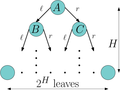
Figure 1: MDP with two actions $\ell$ and $r$, and the true dynamics $M^{\star}$ are shown in the figure. The cost $c(s,a)=\epsilon<<1$ at any $s\neq B$ and $c(B,a)=1$, for any action $a$. Thus, the action taken at $A$ is critical. Model class $\mathcal{M}$ contains only two models: $M^{\mathsf{good}}$ which captures dynamics at $A$ correctly but makes mistakes everywhere else, while $M^{\mathsf{bad}}$ makes mistakes only at $A$ but captures true dynamics everywhere else.

3.2 Challenges in MBRL

We make two important observations from the previous section which directly manifest as the two fundamental challenges in MBRL. We will use Figure 1 to motivate these challenges. First, ensuring that the learned policy $\hat{\pi}_{t}$ satisfies (4) in Algorithm 1 requires performing optimal planning in the learned model $\hat{M}_{t}$ at every iteration. Note that optimal planning can require a number of interactions in $\hat{M}_{t}$ that is exponential in the effective task horizon $\frac{1}{1-\gamma}$ (Kearns et al., 1999). For example in Figure 1, solving for optimal policy requires $\mathcal{O}(2^{H})$ operations. We term this as C1: computational expense challenge in MBRL.

Second, Lemma 3.1 indicates that optimizing terms (2) and (3) (along with (4)) is guaranteed to optimize the performance difference. However, we cannot directly optimize term (3) as it requires access to the value function of the expert in the model $V^{\pi^{\star}}_{\hat{M}}$ which is unknown. To avoid this, MBRL methods bound these terms using model prediction error in Corollary 3.1 as an upper bound that is easy to optimize but very loose, especially due to the unknown scaling term $\|V_{\hat{M}}^{\pi^{\star}}\|_{\infty}$ which can be as large as $\frac{1}{1-\gamma}$. We term this as C2: objective mismatch challenge in MBRL. The model fitting objective of minimizing prediction error is not a good approximation for terms (2) and (3), which are able to capture the relative importance of transition $(s,a)$ in policy computation through the value of the resulting successor. For example in Figure 1, $M^{\mathsf{bad}}$ has lower prediction error than $M^{\mathsf{good}}$ even though it makes a mistake at the crucial state $A$ where the value difference between predicted and true successor is high, while $M^{\mathsf{good}}$ is better according to objective in Lemma 3.1.

4 Performance Difference via Advantage in Model

To overcome the challenges C1 and C2 presented in the previous section, let us revisit the performance difference in Lemma 3.1 and introduce a new decomposition for it that results in a unified objective which is more feasible to optimize. This decomposition is the primary contribution of this paper and we name it as Performance Difference via Advantage in Model (PDAM). The detailed proof can be found in Appendix A.

Lemma 4.1 (Performance Difference via Advantage in Model).

Given any start state distribution $\omega$, policies $\hat{\pi},\pi^{\star}$, and transition functions $\hat{M},M^{\star}$ we have:

$$(1- \gamma)[J_{M^{\star}}^{\omega}(\hat{\pi})-J_{M^{\star}}^{\omega}({\pi^{\star}})]=$$

$$\underbrace{\mathop{{}\mathbb{E}}_{s\sim d_{\omega,{\pi^{\star}}}}[V^{{\hat{\pi}}}_{\hat{M}}(s)-\mathop{{}\mathbb{E}}_{a\sim{\pi^{\star}}(s)}[Q^{{\hat{\pi}}}_{\hat{M}}(s,a)]]}_{\text{Disadvantage on states visited by expert}}$$ (5)

$$+\underbrace{\mathop{{}\gamma\mathbb{E}}_{\begin{subarray}{c}(s,a)\sim D_{\omega,{\hat{\pi}}}\\ s^{\prime}\sim M^{\star}(s,a)\end{subarray}}[V_{\hat{M}}^{{\hat{\pi}}}(s^{\prime})-\mathop{{}\mathbb{E}}_{s^{\prime\prime}\sim\hat{M}(s,a)}[V_{\hat{M}}^{{\hat{\pi}}}(s^{\prime\prime})]]}_{\text{Value difference on states visited by learned policy}}$$ (6)

$$+\underbrace{\mathop{{}\gamma\mathbb{E}}_{\begin{subarray}{c}(s,a)\sim D_{\omega,{\pi^{\star}}}\\ s^{\prime}\sim M^{\star}(s,a)\end{subarray}}[\mathop{{}\mathbb{E}}_{s^{\prime\prime}\sim\hat{M}(s,a)}[V^{{\hat{\pi}}}_{\hat{M}}(s^{\prime\prime})]-V^{{\hat{\pi}}}_{\hat{M}}(s^{\prime})]}_{\text{Value difference on states visited by expert}}$$ (7)

The above lemma presents a novel unified objective for joint model and policy learning. We can make a few important remarks. First, bounding term (5) does not require computing the optimal policy in the learned model $\hat{M}$, unlike term (1). Instead, we need a policy that has small “disadvantage” over the optimal policy in the learned model at states sampled along $\pi^{\star}$ trajectory in $M^{\star}$. This disadvantage term was popularly used as an objective for policy search in several model-free works (Kakade & Langford, 2002; Bagnell et al., 2003; Ross & Bagnell, 2014). Given access to an exploration distribution $\nu$ that covers $D_{\omega,\pi^{\star}}$, computing such a policy requires computation that is polynomial in the effective task horizon (Kakade, 2003), compared to (4) which can require computation that is exponential in the task horizon. In other words, by being “lazy” in the policy computation step we can solve challenge C1 while still optimizing the performance difference between $\hat{\pi}$ and $\pi^{\star}$.

Second, while PDAM looks similar to Lemma 3.1 for the model fitting terms (6) and (7), there is one crucial difference: we only need $V_{\hat{M}}^{\hat{\pi}}$ in the new objective, which is feasible to compute using any policy evaluation method in the learned model (Sutton & Barto, 2018). On the other hand, Lemma 3.1 required access to $V_{\hat{M}}^{\pi^{\star}}$ where $\pi^{\star}$ is unknown and hence, we had to upper bound the objective in Corollary 3.1 using model prediction error. Optimizing prediction error requires the learned model to capture dynamics everywhere equally well. However, the unified objective PDAM offers a “lazy” alternative for model fitting that focuses only on transitions that are critical for policy computation by being value-aware, solving challenge C2.

5 LAMPS: Lazy Model-based Policy Search

Algorithm 3 Minimize Disadvantage ComputePolicy($\hat{M}_{t}$)

0:  Exploration distribution $\nu$, learned model $\hat{M}_{t}$, policy class $\Pi$.

1:  Find $\hat{\pi}_{t}\in\Pi$ using cost-sensitive classification on states sampled from $\nu$ in $\hat{M}_{t}$ (Ross & Bagnell, 2014) such that

$$\mathop{{}\mathbb{E}}_{s\sim\nu}\left[V^{\hat{\pi}_{t}}_{\hat{M}_{t}}(s)-\min_{a\in\mathcal{A}}[Q^{\hat{\pi}_{t}}_{\hat{M}_{t}}(s,a)]\right]\leq\epsilon_{po}$$ (8)

2:  Return $\hat{\pi}_{t}$

In this section, we present our first algorithm LAMPS that uses the unified objective PDAM to solve challenge C1. Algorithm 3 performs policy optimization along the exploration distribution similar to previous policy search methods (Kakade & Langford, 2002; Bagnell et al., 2003; Ross & Bagnell, 2014). Note that (8) requires performing one-step cost-sensitive classification only at states sampled from the exploration distribution $\nu$ making Algorithm 3 computationally efficient. On the other hand, optimal planning requires minimizing disadvantage at all states under the learned policy $d_{\omega,\hat{\pi}_{t}}$ which changes as the learned policy is updated leading to the exponential dependence on horizon.

To understand how Algorithm 3 can help optimize PDAM, we use Hölder’s inequality on terms (6) and (7) to bound PDAM as,

Corollary 5.1.

For any start state distribution $\omega$, transition functions $\hat{M},M^{\star}$, and policies $\hat{\pi},\pi^{\star}$ such that $\hat{\pi}$ satisfies (8), we have,

$$(1-\gamma) [J_{M^{\star}}^{\omega}(\hat{\pi})-J_{M^{\star}}^{\omega}(\pi^{\star})]\leq\epsilon_{po}$$

$$+\gamma\hat{V}_{\max}\mathop{{}\mathbb{E}}_{(s,a)\sim D_{\omega,\hat{\pi}}}\|\hat{M}(s,a)-M^{\star}(s,a)\|_{1}$$

$$+\gamma\hat{V}_{\max}\mathop{{}\mathbb{E}}_{(s,a)\sim D_{\omega,\pi^{\star}}}\|\hat{M}(s,a)-M^{\star}(s,a)\|_{1}$$

where $\hat{V}_{\max}=\|V_{\hat{M}}^{\hat{\pi}}\|_{\infty}$.

Corollary 5.1 indicates a simple modification to existing MBRL methods where we use MLE-based Algorithm 2 for model fitting and Algorithm 3 for policy computation in the framework of Algorithm 1. We refer to this new algorithm as LAMPS. Note that by upper bounding the model fitting terms in Lemma 4.1 using model prediction error, LAMPS is only able to solve challenge C1 but not C2.

Our algorithm only requires an exploration distribution $\nu$ that covers the expert policy state-action distribution $D_{\omega,\pi^{\star}}$ as described in Section 3. To capture how well $\nu$ covers $D_{\omega,\pi^{\star}}$, we define the coverage coefficient $\mathcal{C}=\sup_{s,a}\frac{D_{\omega,\pi^{\ast}}(s,a)}{\nu(s,a)}$ similar to Ross & Bagnell (2012). We now present the regret bound for LAMPS using this coverage coefficient and proof can be found in Appendix A.

Theorem 5.1.

Let $\{\hat{\pi}_{t}\}^{T}_{t=1}$ be the sequence of returned policies of LAMPS. We have: 

$$\frac{1}{T}\sum_{t=1}^{T} J_{M^{\star}}^{\omega}(\hat{\pi}_{t})-J_{M^{\star}}^{\omega}(\pi^{\star})\leq$$

$$\tilde{O}\left(\mathcal{C}\epsilon_{po}+\frac{\mathcal{C}\hat{V}_{\max}}{1-\gamma}\left(\sqrt{\epsilon^{KL}_{model}}+\frac{1}{\sqrt{T}}\right)\right),$$

where $\hat{V}_{\max}=\|V^{\hat{\pi}}_{\hat{M}}\|_{\infty}$, $\mathcal{C}=\sup_{s,a}\frac{D_{\omega,\pi^{\ast}}(s,a)}{\nu(s,a)}$ is the coverage coefficient, $\epsilon_{po}$ is the policy advantage error, and $\epsilon^{KL}_{model}=\min_{M\in\mathcal{M}}\mathop{{}\mathbb{E}}_{s,a\sim\bar{\mathcal{D}}_{T}}\mathsf{KL}(M(s,a),M^{\ast}(s,a))$ is the agnostic model error.

In comparison, Ross & Bagnell (2012)’s regret bound is

$$\tilde{O}\left(\epsilon_{oc}+\frac{\mathcal{C}\max\{V_{\max},\hat{V}_{\max}\}}{1-\gamma}\left(\sqrt{\epsilon^{KL}_{model}}+\frac{1}{\sqrt{T}}\right)\right),$$

where $V_{\max}=\|V^{\pi^{\ast}}_{\hat{M}}\|_{\infty}$ is difficult to optimize as $\pi^{\star}$ is unknown, and can be as large as the effective horizon $\frac{1}{1-\gamma}$. On the other hand, our bound only has $\hat{V}_{\max}=\|V^{\hat{\pi}}_{\hat{M}}\|_{\infty}$ which is optimized in Algorithm 3 for states that are sampled from $\nu$. Thus, we expect that there exists cases where $\hat{V}_{\max}$ is much smaller when compared to $V_{\max}$, leading to a tighter regret bound in Theorem 5.1. Hence, while LAMPS primarily solves challenge C1 lending computational gains, we also observe statistical gains in practice as we show in our experiments in Section 7. Another crucial difference is that the coverage coefficient $\mathcal{C}$ shows up for the policy optimization error in LAMPS regret bound which suggests that LAMPS is relatively more sensitive to the quality of exploration distribution $\nu$. We show an example of this in Appendix C.2.

Algorithm 4 Moment Matching FitModel($\mathcal{D}_{t},\{\ell_{i}\}_{i=1}^{t-1}$)

0:  Data $\mathcal{D}_{t}$, model class $\mathcal{M}$, previous losses $\{\ell_{i}\}_{i=1}^{t-1}$, Strongly convex regularizer $\mathcal{R}$

1:  Define loss

$$\ell_{t}(M)=\mathop{{}\mathbb{E}}_{(s,a,s^{\prime})\sim\mathcal{D}_{t}}\left|V^{\hat{\pi}_{t}}_{\hat{M}_{t}}(s^{\prime})-\mathop{{}\mathbb{E}}_{s^{\prime\prime}\sim M(s,a)}[V^{\hat{\pi}_{t}}_{\hat{M}_{t}}(s^{\prime\prime})]\right|$$ (9)

2:  Compute model $\hat{M}_{t+1}$ using an online no-regret algorithm, such as FTRL (Hazan, 2019),

$$\hat{M}_{t+1}\leftarrow\mathop{\mathrm{argmin}}_{M\in\mathcal{M}}\sum_{\tau=1}^{t}\ell_{\tau}(M)+\mathcal{R}(M).$$ (10)

3:  Return $\hat{M}_{t+1}$

6 LAMPS-MM: Lazy Model-based Policy Search via Value Moment Matching

The previous section introduced an algorithm LAMPS that, while being more computationally efficient than existing MBRL methods, did not reap the full benefits of our proposed unified objective PDAM. LAMPS optimizes the objective presented in Corollary 5.1 which is a weak upper bound of the unified objective (as explained in Section 3.2.) A natural question would be to ask whether there exists an algorithm that directly optimizes the unified objective without constructing a weak upper bound. We present such an algorithm in this section. The key idea is to formulate it as a moment matching problem (Sun et al., 2019b; Swamy et al., 2021) where our learned model is matching the true dynamics in expectation using value moments.

Algorithm 4 minimizes the value moment difference between true and predicted successors on a given dataset of transitions. The objective $\ell_{t}$ in (9) upper bounds the terms (6) and (7), and using a Follow-the-Regularized-Leader (FTRL) approach with a strongly convex regularizer $\mathcal{R}(M)$ allows us to achieve a no-regret guarantee. We refer to the new MBRL algorithm that uses value moment matching based Algorithm 4 for model fitting and Algorithm 3 for policy computation in the framework of Algorithm 1 as LAMPS-MM.

LAMPS-MM, by virtue of optimizing PDAM, does not suffer challenge C2 as the model fitting objective helps learn models that are useful for policy computation by focusing on critical states where any mistake in action can lead to large value differences. Going back to the example in Figure 1, LAMPS-MM would pick $M^{\mathsf{good}}$ over $M^{\mathsf{bad}}$ as the latter incurs high loss $\ell_{t}$ (9) at state $A$. Thus, LAMPS-MM solves both challenges C1 and C2. This results in improved statistical efficiency as indicated by its tighter regret bound:

Theorem 6.1.

Let $\{\hat{\pi}_{t}\}^{T}_{t=1}$ be the sequence of returned policies of LAMPS-MM, we have:

$$\frac{1}{T}\sum_{t=1}^{T}J_{M^{\star}}^{\omega}(\hat{\pi}_{t}) -J_{M^{\star}}^{\omega}(\pi^{\star})\leq$$

$$\tilde{O}\left(\mathcal{C}\epsilon_{po}+\frac{\mathcal{C}}{1-\gamma}\left(\epsilon^{mm}_{model}+\frac{1}{\sqrt{T}}\right)\right),$$

where $\epsilon^{mm}_{model}=\min_{M\in\mathcal{M}}\frac{1}{T}\sum_{t=1}^{T}\ell_{t}(M)$ is the agnostic model error, $\epsilon_{po}$ is the policy advantage error, and $\mathcal{C}=\sup_{s,a}\frac{D_{\omega,\pi^{\ast}}(s,a)}{\nu(s,a)}$ is the coverage coefficient.

Comparing the above regret bound with that of LAMPS in Theorem 5.1, we have improved the bound by getting rid of the dependency on $\hat{V}_{\max}$ which as stated in Section 5, can be as large as $\frac{1}{1-\gamma}$ in the worst case.

Despite the statistical advantages of LAMPS-MM, its practical implementation is difficult as estimating the loss $\ell_{t}$ (9) requires evaluating the policy in the learned model which can only be approximated in large MDPs. A similar difficulty was also observed in previous works (Ayoub et al., 2020; Grimm et al., 2020; Farahmand et al., 2017) that proposed value-aware objectives for model fitting. We highlight a few scenarios in which Algorithm 4 is practically realizable. First, for finite MDPs we can evaluate the policy exactly avoiding this difficulty. Second, in MDPs such as linear dynamical systems with quadratic costs where we can compute the value of policy in closed form, we can estimate $\ell_{t}$ and use a gradient-based optimization method to find the best model in the model class in the optimization problem (10). We demonstrate both of these scenarios in our experiments in Section 7. It is also important to note that solving (10) using a batch algorithm, like gradient descent, would require aggregating both data $\mathcal{D}_{t}$ and value functions $\hat{V}^{\hat{\pi}_{t}}_{\hat{M}_{t}}$ across iterations in Algorithm 1. This is advantageous as our approach does not require us to compute gradients through how changes in model $M$ affect the value estimates used in $\ell_{t}(M)$ (see (9)) which can be very difficult to compute.

For completeness, we also give a finite sample analysis for LAMPS-MM in Appendix B.3. Note that we skip the finite sample analysis for LAMPS, because the analysis takes the same form as Ross & Bagnell (2012).

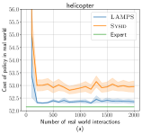
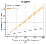
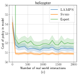
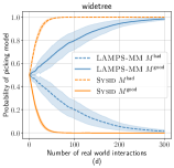
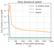
Figure 2: Results on our Helicopter, WideTree, and Linear Dynamical System (LDS) Domains. All experiments are done using $10$ random seeds and the solid lines show the mean while shaded area depicts standard error. For helicopter and LDS experiments at each iteration, we add $100$ samples, that are sampled with equal probability from exploration distribution and learned policy rollouts, to the dataset.

7 Experiments

In this section, we present experiments that test our proposed algorithms against baselines across five varied domains. For baselines, we compare with Ross & Bagnell (2012) that uses MLE for model fitting and optimal planning for policy computation, and call this baseline as SysID. In addition to this, we also use MBPO (Janner et al., 2019) and design variants of it that utilize exploration distribution, similar to SysID, to ensure a fair comparison with our proposed algorithms. We defer details of our experiment setup, cost functions, and baseline implementation to Appendix C.

7.1 Helicopter

In this domain from Ross & Bagnell (2012), we compare LAMPS with SysID. The objective of the task is for the helicopter to track a desired trajectory with unknown dynamics under the presence of noise. For both approaches, we use an exploration distribution $\nu$ that samples from the desired trajectory. For optimal planning in SysID, we run iLQR (Li & Todorov, 2004) until convergence, and to implement Algorithm 3 for LAMPS we run a single iteration of iLQR where the forward pass is replaced with the desired trajectory and we run a single LQR backward pass on it to compute the policy. For detailed explanation on the dynamics, cost function, and implementations of SysID and LAMPS, refer to Appendix C.1.1.

Figure 2(a) shows that LAMPS can learn a better policy than SysID given the same amount of real world data and the same exploration distribution, indicating statistical gains. To test our hypothesis that this is due to the tighter regret bound for LAMPS as $\hat{V}_{\max}<V_{\max}$, Figure 2(c) shows how the learned policy $\hat{\pi}$ performs in the learned model $\hat{M}$ for both approaches, and the expert’s performance in $\hat{M}$. Observe that both LAMPS and SysID are able to optimize $V^{\hat{\pi}}_{\hat{M}}$ but the expert’s performance $V_{\hat{M}}^{\pi^{\star}}$ is not optimized as well leading to a weaker regret bound for SysID when compared to LAMPS. Figure 2(b) shows the computational benefits of LAMPS where we plot the number of LQR solver calls, the most expensive operation, made by each approach and we can observe that by only optimizing on the exploration distribution LAMPS significantly outperforms SysID in the amount of computation used.

7.2 WideTree

We use a variant of the finite MDP domain introduced in Ayoub et al. (2020) that is very similar to Figure 1 with $H=3$. The model class consists of two models: $M^{\mathsf{good}}$ and $M^{\mathsf{bad}}$ as described in Figure 1. For detailed explanation of the dynamics, refer to  Figure 5 in Appendix C.1.2. We compare LAMPS-MM and SysID. To compute the best model to pick at every iteration given the data so far, we use Hedge (Freund & Schapire, 1997) to update the discrete probability distribution over the two models. Figure 2(d) shows how the distribution evolves when using MLE-based model fitting loss in SysID and value moment matching loss in LAMPS-MM. As $M^{\mathsf{bad}}$ matches true dynamics everywhere except at the root, SysID collapses to a distribution that picks the bad model over a good model always, while LAMPS-MM which reasons about the usefulness of transitions in computing good policies converges to a distribution that picks the good model more often.

7.3 Linear Dynamical System

In this experiment, we use a simple linear dynamical system with quadratic costs over a finite horizon as our domain (similar to LQR) for which we can compute the value function in closed form. The real world has time-varying linear dynamics while the model class only has time-invariant linear models making it agnostic. The cost function penalizes control input at every timestep and the state only at the final timestep (no intermediate state costs.) For detailed explanation on the dynamics, cost functions, and model fitting losses, refer to  Appendix C.1.3. Figure 2(e) shows the results for LAMPS-MM and SysID. SysID converges slowly to the expert performance trying to match the true dynamics at every timestep while LAMPS-MM using the value moment matching objective quickly realizes that only the final state matters for cost and finds a simple model which results in controls that bring the state to zero by the end of the horizon. Thus, we see that LAMPS-MM by being value-aware can achieve significant statistical gains over traditional MBRL methods.

7.4 Mujoco Locomotion Benchmarks

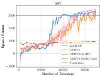
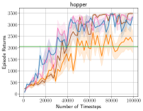
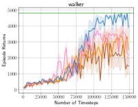
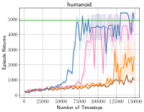
Figure 3: Results on mujoco locomotion benchmarks. All experiments are done using 5 random seeds and the shaded area denotes the standard error. We use 50000 exploration samples for humanoid task, and 10000 samples for all the other tasks. MBPO also uses 10000 random exploration samples as warm-start. The baseline “Exploration” denotes the average episodic returns of the exploration dataset.

In this experiment we test LAMPS on the standard dense reward mujoco benchmarks (Brockman et al., 2016). All baselines are implemented based on MBPO (Janner et al., 2019). In addition to MBPO, we also design a variant MBPO-SysID which also uses data from exploration distribution, similar to SysID, for model fitting. The branched update in MBPO serves as an efficient surrogate for optimal planning in MBPO-SysID. Another variant MBPO-SysID (2x) doubles the number of policy updates and the number of interactions with the learned model used when compared to MBPO-SysID. For LAMPS, we keep the model fitting procedure the same as MBPO-SysID and use states sampled from the exploration distribution for policy updates, rather than the current policy’s visitation distribution. For the exploration distribution $\nu$, we use an offline dataset and sample from it every iteration. For more details on implementation such as hyperparameters, refer to Appendix C.3.

We show the results in Figure 3. Compared to MBPO, both LAMPS and MBPO-SysID show better statistical efficiency, which highlights the advantage of exploration distribution (Ross & Bagnell, 2012). We note that LAMPS consistently finds better policies with less number of real world interactions than MBPO-SysID across all environments, especially in humanoid which is the most difficult environment among the ones used. The performance of MBPO-SysID (2x) shows that even when equipped with twice the amount of computation as LAMPS, LAMPS still outperforms or is competitive in all experiments. This highlights both the computational and statistical efficiency of LAMPS.

7.5 Maze

Our final experiment investigates the performance of LAMPS in sparse reward task by using PointMaze environment (Fu et al., 2020) as the domain. We use only a small subset of the offline dataset as the exploration distribution resulting in partial coverage and a small number of expert trajectories. More details in Appendix C.1.4. Since LAMPS uses the exploration distribution in both model fitting and policy computation steps, we expect it to outperform MBPO-SysID, which only uses it in model fitting, as intelligent exploration is necessary in sparse reward settings. Figure 4 confirms our hypothesis where LAMPS outperforms MBPO-SysID by a significant margin. By focusing policy computation only along exploration distribution, LAMPS does not exploit any inaccuracies elsewhere in the learned model and quickly converges to a good policy.

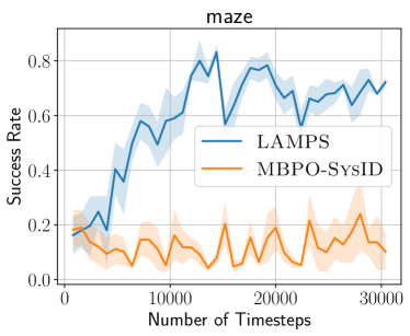
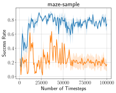
Figure 4: Results on D4RL PointMaze (large) environment. We use 10000 exploration samples (left) and 50000 samples (right). In both setups, our algorithm shows a better exploration ability even though neither approach utilizes an explicit exploration scheme such as an exploration bonus. The results are averaged over 5 random seeds and the shaded area denotes the standard error.

8 Discussion

In this work, we introduce a new unified objective function for MBRL. The proposed objective function is designed to improve computational efficiency in policy computation and alleviate the objective mismatch issue in model fitting. Additionally, we present two no-regret algorithms, LAMPS and LAMPS-MM, that leverage the proposed objective function and demonstrate their effectiveness through statistical and computational gains on simulated benchmarks.

However, it should be noted that while LAMPS is relatively straightforward to implement, LAMPS-MM may be challenging to apply to large MDPs where exact policy evaluation is difficult. Additionally, both algorithms are sensitive to the quality of exploration distribution $\nu$, and can only guarantee small regret against policies with state-action distribution close to $\nu$. Hence, we can expect these algorithms to compute a good policy if our prior knowledge of the task allows us to design good exploration distributions.

An interesting future work would be to extend this to the latent model setting, where we learn dynamics over an underlying latent state. In such a setting, the typical MLE model fitting objective does not intuitively make sense as we do not observe the underlying state and only have access to raw observations. We would also like to investigate if there exists a “doubly-robust” version that combines the best of SysID and LAMPS where we can take advantage of either having a good exploration distribution or a computationally cheap optimal planner.

Appendix A Proofs

A.1 Proofs for Section 3.1

The simulation lemma is useful to relate the performance of any policy $\pi$, between two models, for example, the learned model $\hat{M}$ and the real model $M^{\ast}$:

Lemma A.1 (Simulation Lemma).

For any start distribution $\omega$, policy $\pi$, and transition functions $\hat{M}$, $M^{\star}$, we have

$$J_{M^{\star}}^{\omega}(\pi)-J_{\hat{M}}^{\omega}(\pi)=\mathbb{E}_{s\sim\omega}[V^{\pi}_{M^{\star}}(s)-V^{\pi}_{\hat{M}}(s)]$$

$$=\frac{\gamma}{1-\gamma}\mathbb{E}_{(s,a)\sim D_{\omega,\pi}}\left[\mathbb{E}_{s^{\prime}\sim M^{\star}(s,a)}[V^{\pi}_{\hat{M}}(s^{\prime})]-\mathbb{E}_{s^{\prime\prime}\sim\hat{M}(s,a)}[V^{\pi}_{\hat{M}}(s^{\prime\prime})]\right]$$ (11)

Proof.

The first equality follows from the definition of $J^{\omega}_{M}(\pi)$ as defined in Section 3. To prove the second equality we establish a recurrence as follows:

$$\mathbb{E}_{s\sim\omega}[V^{\pi}_{M^{\star}}(s)-V^{\pi}_{\hat{M}}(s)]$$

$$=\mathop{{}\mathbb{E}}_{s\sim\omega,a\sim\pi(s)}[c(s,a)+\gamma\mathop{{}\mathbb{E}}_{s^{\prime}\sim M^{\star}(s,a)}[V^{\pi}_{M^{\star}}(s^{\prime})]-c(s,a)-\gamma\mathop{{}\mathbb{E}}_{s^{\prime\prime}\sim\hat{M}(s,a)}[V^{\pi}_{\hat{M}}(s^{\prime\prime})]]$$

$$=\gamma\mathop{{}\mathbb{E}}_{s\sim\omega,a\sim\pi(s)}[\mathop{{}\mathbb{E}}_{s^{\prime}\sim M^{\star}(s,a)}[V^{\pi}_{M^{\star}}(s^{\prime})]-\mathop{{}\mathbb{E}}_{s^{\prime\prime}\sim\hat{M}(s,a)}[V^{\pi}_{\hat{M}}(s^{\prime\prime})]]$$

$$=\gamma\mathop{{}\mathbb{E}}_{s\sim\omega,a\sim\pi(s)}[\mathop{{}\mathbb{E}}_{s^{\prime}\sim M^{\star}(s,a)}[V^{\pi}_{M^{\star}}(s^{\prime})]-\mathop{{}\mathbb{E}}_{s^{\prime}\sim M^{\star}(s,a)}[V^{\pi}_{\hat{M}}(s^{\prime})]+\mathop{{}\mathbb{E}}_{s^{\prime}\sim M^{\star}(s,a)}[V^{\pi}_{\hat{M}}(s^{\prime})]-\mathop{{}\mathbb{E}}_{s^{\prime\prime}\sim\hat{M}(s,a)}[V^{\pi}_{\hat{M}}(s^{\prime\prime})]]$$

$$=\gamma\mathop{{}\mathbb{E}}_{s^{\prime}\sim d_{\omega,\pi}^{1}}[V^{\pi}_{M^{\star}}(s^{\prime})-V^{\pi}_{\hat{M}}(s^{\prime})]+\gamma\mathop{{}\mathbb{E}}_{(s,a)\sim D^{0}_{\omega,\pi}}\left[\mathbb{E}_{s^{\prime}\sim M^{\star}(s,a)}[V^{\pi}_{\hat{M}}(s^{\prime})]-\mathbb{E}_{s^{\prime\prime}\sim\hat{M}(s,a)}[V^{\pi}_{\hat{M}}(s^{\prime\prime})]\right]$$

Thus, we established a recurrence between the performance difference at time $0$ and the performance difference at time $1$ with the state sampled from the state distribution by following $\pi$ at time $1$. We can solve this recurrence for the infinite horizon to get the lemma statement. ∎

The Performance difference via Planning in Model (PDPM) lemma is as follows:

Lemma A.2 (PDPM (Lemma 3.1 restate)).

For any start state distribution $\omega$, policies $\hat{\pi}$, $\pi^{\star}$, and transition functions $\hat{M},M^{\star}$ we have,

$$J_{M^{\star}}^{\omega}(\hat{\pi})-J_{M^{\star}}^{\omega}(\pi^{\star})=\mathbb{E}_{s\sim\omega}[V_{M^{\star}}^{\hat{\pi}}(s)-V_{M^{\star}}^{\pi^{\star}}(s)]= \mathbb{E}_{s\sim\omega}[V^{\hat{\pi}}_{\hat{M}}(s)-V^{\pi^{\star}}_{\hat{M}}(s)]$$

$$+\frac{\gamma}{1-\gamma}\mathbb{E}_{(s,a)\sim D_{\omega,\hat{\pi}}}[\mathop{{}\mathbb{E}}_{s^{\prime}\sim M^{\star}(s,a)}[V_{\hat{M}}^{\hat{\pi}}(s^{\prime})]-\mathop{{}\mathbb{E}}_{s^{\prime\prime}\sim\hat{M}(s,a)}[V_{\hat{M}}^{\hat{\pi}}(s^{\prime\prime})]]$$

$$+\frac{\gamma}{1-\gamma}\mathbb{E}_{(s,a)\sim D_{\omega,\pi^{\star}}}[\mathop{{}\mathbb{E}}_{s^{\prime\prime}\sim\hat{M}(s,a)}[V_{\hat{M}}^{\pi^{\star}}(s^{\prime\prime})]-\mathop{{}\mathbb{E}}_{s^{\prime}\sim M^{\star}(s,a)}[V_{\hat{M}}^{\pi^{\star}}(s^{\prime})]]$$

Proof.

We can add and subtract terms on the left hand side to get

$$\mathbb{E}_{s\sim\omega}[V_{M^{\star}}^{\hat{\pi}}(s)-V_{M^{\star}}^{\pi^{\star}}(s)]=$$

$$\mathbb{E}_{s\sim\omega}\left[(V^{\hat{\pi}}_{\hat{M}}(s)-V_{\hat{M}}^{\pi^{\star}}(s))+(V^{\hat{\pi}}_{M^{\star}}(s)-V^{\hat{\pi}}_{\hat{M}}(s))+(V^{\pi^{\star}}_{\hat{M}}(s)-V^{\pi^{\star}}_{M^{\star}}(s))\right]$$

Apply the simulation lemma to the second and third terms inside the expectation above to get the result

$$\mathbb{E}_{s\sim\omega}[V_{M^{\star}}^{\hat{\pi}}(s)-V_{M^{\star}}^{\pi^{\star}}(s)] =\mathbb{E}_{s\sim\omega}[V^{\hat{\pi}}_{\hat{M}}(s)-V^{\pi^{\star}}_{\hat{M}}(s)]$$

$$+\frac{\gamma}{1-\gamma}\mathbb{E}_{(s,a)\sim d_{\omega,\hat{\pi}},s^{\prime}\sim M^{\star}(s,a),s^{\prime\prime}\sim\hat{M}(s,a)}[V_{\hat{M}}^{\hat{\pi}}(s^{\prime})-V_{\hat{M}}^{\hat{\pi}}(s^{\prime\prime})]$$

$$+\frac{\gamma}{1-\gamma}\mathbb{E}_{(s,a)\sim d_{\omega,\pi^{\star}},s^{\prime}\sim M^{\star}(s,a),s^{\prime\prime}\sim\hat{M}(s,a)}[V_{\hat{M}}^{\pi^{\star}}(s^{\prime\prime})-V_{\hat{M}}^{\pi^{\star}}(s^{\prime})]$$

∎

Corollary A.1 (Corollary 3.1 restate).

For any start state distribution $\omega$, $\pi^{\star}$, and transition functions $\hat{M},M^{\star}$, let $\hat{\pi}$ be the returned optimal control policy in $\hat{M}$ as in (4), we have,

$$\mathbb{E}_{s\sim\omega} [V_{M^{\star}}^{\hat{\pi}}(s)-V_{M^{\star}}^{\pi^{\star}}(s)]\leq\epsilon_{oc}+$$

$$\frac{\gamma\hat{V}_{\max}}{1-\gamma}\mathbb{E}_{(s,a)\sim D_{\omega,\hat{\pi}}}\left\|\hat{M}(s,a)-M^{\star}(s,a)\right\|_{1}+$$

$$\frac{\gamma V_{\max}}{1-\gamma}\mathbb{E}_{(s,a)\sim D_{\omega,\pi^{\star}}}\left\|\hat{M}(s,a)-M^{\star}(s,a)\right\|_{1},$$

where $\hat{V}_{\max}=\|V_{\hat{M}}^{\hat{\pi}}\|_{\infty},V_{\max}=\|V^{\pi^{\ast}}_{\hat{M}}\|_{\infty}$.

Proof.

By Lemma 3.1, we have:

$$\mathbb{E}_{s\sim\omega}[V_{M^{\star}}^{\hat{\pi}}(s)-V_{M^{\star}}^{\pi^{\star}}(s)] =\mathbb{E}_{s\sim\omega}[V^{\hat{\pi}}_{\hat{M}}(s)-V^{\pi^{\star}}_{\hat{M}}(s)]$$

$$+\frac{\gamma}{1-\gamma}\mathbb{E}_{(s,a)\sim d_{\omega,\hat{\pi}},s^{\prime}\sim M^{\star}(s,a),s^{\prime\prime}\sim\hat{M}(s,a)}[V_{\hat{M}}^{\hat{\pi}}(s^{\prime})-V_{\hat{M}}^{\hat{\pi}}(s^{\prime\prime})]$$

$$+\frac{\gamma}{1-\gamma}\mathbb{E}_{(s,a)\sim d_{\omega,\pi^{\star}},s^{\prime}\sim M^{\star}(s,a),s^{\prime\prime}\sim\hat{M}(s,a)}[V_{\hat{M}}^{\pi^{\star}}(s^{\prime\prime})-V_{\hat{M}}^{\pi^{\star}}(s^{\prime})],$$

Then we bound the first term by (4), and by holder’s inequality, the second term is bounded by

$$\frac{\gamma}{1-\gamma}\mathbb{E}_{(s,a)\sim d_{\omega,\hat{\pi}},s^{\prime}\sim M^{\star}(s,a),s^{\prime\prime}\sim\hat{M}(s,a)}[V_{\hat{M}}^{\hat{\pi}}(s^{\prime})-V_{\hat{M}}^{\hat{\pi}}(s^{\prime\prime})]\leq\frac{\gamma}{1-\gamma}\|V_{\hat{M}}^{\hat{\pi}}\|_{\infty}\mathbb{E}_{s,a\sim D_{\omega,\hat{\pi}}}\left\|\hat{M}(s,a)-M^{\star}(s,a)\right\|_{1},$$

and apply holder’s inequality to the third term similarly, we complete the proof. ∎

A.2 Proofs for Section 4

In this section, we present the proof for Section 4. Let us start with the Performance Difference via Advantage in Model (PDAM) Lemma:

Lemma A.3 (PDAM (restate of Lemma 4.1)).

Given any start state distribution $\omega$, policies $\hat{\pi},\pi^{\star}$, and transition functions $\hat{M},M^{\star}$ we have:

$$J_{M^{\star}}^{\omega}(\hat{\pi})-J_{M^{\star}}^{\omega}(\pi^{\star})=\mathbb{E}_{s\sim\omega}[V_{M^{\star}}^{\hat{\pi}}(s)-V_{M^{\star}}^{\pi^{\star}}(s)]=$$

$$\frac{\gamma}{1-\gamma}\mathbb{E}_{(s,a)\sim D_{\omega,\hat{\pi}}}[\mathop{{}\mathbb{E}}_{s^{\prime}\sim M^{\star}(s,a)}[V_{\hat{M}}^{\hat{\pi}}(s^{\prime})]-\mathop{{}\mathbb{E}}_{s^{\prime\prime}\sim\hat{M}(s,a)}[V_{\hat{M}}^{\hat{\pi}}(s^{\prime\prime})]]+$$

$$\frac{\gamma}{1-\gamma}\mathop{{}\mathbb{E}}_{(s,a)\sim D_{\omega,\pi^{\star}}}[\mathop{{}\mathbb{E}}_{s^{\prime\prime}\sim\hat{M}(s,a)}[V^{\hat{\pi}}_{\hat{M}}(s^{\prime\prime})]-\mathop{{}\mathbb{E}}_{s^{\prime}\sim M^{\star}(s,a)}[V^{\hat{\pi}}_{\hat{M}}(s^{\prime})]]+$$

$$\frac{1}{1-\gamma}\mathop{{}\mathbb{E}}_{s\sim d_{\omega,\pi^{\star}}}[V^{\hat{\pi}}_{\hat{M}}(s)-\mathop{{}\mathbb{E}}_{a\sim\pi^{\star}(s)}[Q^{\hat{\pi}}_{\hat{M}}(s,a)]]$$

Proof.

Let’s begin with the left hand side, and reformulate it as follows:

$$\mathbb{E}_{s\sim\omega}[V_{M^{\star}}^{\hat{\pi}}(s)-V^{\pi^{\star}}_{M^{\star}}(s)]=\mathbb{E}_{s\sim\omega}[V^{\hat{\pi}}_{\hat{M}}(s)-V_{M^{\star}}^{\pi^{\star}}(s)]+\mathbb{E}_{s\sim\omega}[V^{\hat{\pi}}_{M^{\star}}(s)-V^{\hat{\pi}}_{\hat{M}}(s)]$$

The second term above is familiar to us, it is the left hand side of the simulation lemma in equation (11). So we can apply the simulation lemma to get:

$$\mathbb{E}_{s\sim\omega}[V_{M^{\star}}^{\hat{\pi}}(s)-V^{\pi^{\star}}_{M^{\star}}(s)]=\mathbb{E}_{s\sim\omega}[V^{\hat{\pi}}_{\hat{M}}(s)-V_{M^{\star}}^{\pi^{\star}}(s)]+\frac{\gamma}{1-\gamma}\mathbb{E}_{(s,a)\sim D_{\omega,\hat{\pi}}}\left[\mathbb{E}_{s^{\prime}\sim M^{\star}(s,a)}[V^{\hat{\pi}}_{\hat{M}}(s^{\prime})]-\mathbb{E}_{s^{\prime\prime}\sim\hat{M}(s,a)}[V^{\hat{\pi}}_{\hat{M}}(s^{\prime\prime})]\right]$$ (12)

Now all that remains is the first term which can be simplified as:

$$\mathop{{}\mathbb{E}}_{s\sim\omega}[V^{\hat{\pi}}_{\hat{M}}(s)-V^{\pi^{\star}}_{M^{\star}}(s)]$$

$$=\mathop{{}\mathbb{E}}_{s\sim\omega}[V^{\hat{\pi}}_{\hat{M}}(s)-\mathop{{}\mathbb{E}}_{a\sim\pi^{\star}(s)}Q^{\hat{\pi}}_{\hat{M}}(s,a)+\mathop{{}\mathbb{E}}_{a\sim\pi^{\star}(s)}Q^{\hat{\pi}}_{\hat{M}}(s,a)-V^{\pi^{\star}}_{M^{\star}}(s)]$$

$$=\mathop{{}\mathbb{E}}_{s\sim\omega}[V^{\hat{\pi}}_{\hat{M}}(s)-\mathop{{}\mathbb{E}}_{a\sim\pi^{\star}(s)}Q^{\hat{\pi}}_{\hat{M}}(s,a)]$$

$$~{}~{}~{}~{}+\mathop{{}\mathbb{E}}_{s\sim\omega}\left[\mathop{{}\mathbb{E}}_{a\sim\pi^{\star}(s)}[c(s,a)+\gamma\mathop{{}\mathbb{E}}_{s^{\prime\prime}\sim\hat{M}(s,a)}V^{\hat{\pi}}_{\hat{M}}(s^{\prime\prime})]\right.$$

$$~{}~{}~{}~{}~{}~{}~{}~{}-\left.\mathop{{}\mathbb{E}}_{a\sim\pi^{\star}(s)}[c(s,a)+\gamma\mathop{{}\mathbb{E}}_{s^{\prime}\sim M^{\star}(s,a)}V^{\pi^{\star}}_{M^{\star}}(s^{\prime})]\right]$$

$$=\mathop{{}\mathbb{E}}_{s\sim\omega}[V^{\hat{\pi}}_{\hat{M}}(s)-\mathop{{}\mathbb{E}}_{a\sim\pi^{\star}(s)}Q^{\hat{\pi}}_{\hat{M}}(s,a)]$$

$$~{}~{}~{}~{}+\gamma\mathop{{}\mathbb{E}}_{(s,a)\sim D_{\omega,\pi^{\star}}^{0}}[\mathop{{}\mathbb{E}}_{s^{\prime\prime}\sim\hat{M}(s,a)}V^{\hat{\pi}}_{\hat{M}}(s^{\prime\prime})-\mathop{{}\mathbb{E}}_{s^{\prime}\sim M^{\star}(s,a)}V^{\pi^{\star}}_{M^{\star}}(s^{\prime})]$$

$$=\mathop{{}\mathbb{E}}_{s\sim\omega}[V^{\hat{\pi}}_{\hat{M}}(s)-\mathop{{}\mathbb{E}}_{a\sim\pi^{\star}(s)}Q^{\hat{\pi}}_{\hat{M}}(s,a)]$$

$$~{}~{}~{}~{}+\gamma\mathop{{}\mathbb{E}}_{(s,a)\sim D_{\omega,\pi^{\star}}^{0}}\left[\mathop{{}\mathbb{E}}_{s^{\prime\prime}\sim\hat{M}(s,a)}V^{\hat{\pi}}_{\hat{M}}(s^{\prime\prime})-\mathop{{}\mathbb{E}}_{s^{\prime}\sim M^{\star}(s,a)}V^{\hat{\pi}}_{\hat{M}}(s^{\prime})\right.$$

$$~{}~{}~{}~{}~{}~{}~{}~{}+\left.\mathop{{}\mathbb{E}}_{s^{\prime}\sim M^{\star}(s,a)}V^{\hat{\pi}}_{\hat{M}}(s^{\prime})-\mathop{{}\mathbb{E}}_{s^{\prime}\sim M^{\star}(s,a)}V^{\pi^{\star}}_{M^{\star}}(s^{\prime})\right]$$

$$=\mathop{{}\mathbb{E}}_{s\sim\omega}[V^{\hat{\pi}}_{\hat{M}}(s)-\mathop{{}\mathbb{E}}_{a\sim\pi^{\star}(s)}Q^{\hat{\pi}}_{\hat{M}}(s,a)]$$

$$~{}~{}~{}~{}+\gamma\mathop{{}\mathbb{E}}_{(s,a)\sim D_{\omega,\pi^{\star}}^{0}}[\mathop{{}\mathbb{E}}_{s^{\prime\prime}\sim\hat{M}(s,a)}V^{\hat{\pi}}_{\hat{M}}(s^{\prime\prime})-\mathop{{}\mathbb{E}}_{s^{\prime}\sim M^{\star}(s,a)}V^{\hat{\pi}}_{\hat{M}}(s^{\prime})]$$

$$~{}~{}~{}~{}+\gamma\mathop{{}\mathbb{E}}_{(s,a)\sim D_{\omega,\pi^{\star}}^{0}}[\mathop{{}\mathbb{E}}_{s^{\prime}\sim M^{\star}(s,a)}V^{\hat{\pi}}_{\hat{M}}(s^{\prime})-\mathop{{}\mathbb{E}}_{s^{\prime}\sim M^{\star}(s,a)}V^{\pi^{\star}}_{M^{\star}}(s^{\prime})]$$

$$=\mathop{{}\mathbb{E}}_{s\sim\omega}[V^{\hat{\pi}}_{\hat{M}}(s)-\mathop{{}\mathbb{E}}_{a\sim\pi^{\star}(s)}Q^{\hat{\pi}}_{\hat{M}}(s,a)]$$

$$~{}~{}~{}~{}+\gamma\mathop{{}\mathbb{E}}_{(s,a)\sim D_{\omega,\pi^{\star}}^{0}}[\mathop{{}\mathbb{E}}_{s^{\prime\prime}\sim\hat{M}(s,a)}V^{\hat{\pi}}_{\hat{M}}(s^{\prime\prime})-\mathop{{}\mathbb{E}}_{s^{\prime}\sim M^{\star}(s,a)}V^{\hat{\pi}}_{\hat{M}}(s^{\prime})]$$

$$~{}~{}~{}~{}+\gamma\mathop{{}\mathbb{E}}_{s^{\prime}\sim d_{\omega,\pi^{\star}}^{1}}[V^{\hat{\pi}}_{\hat{M}}(s^{\prime})-V^{\pi^{\star}}_{M^{\star}}(s^{\prime})]$$

Solving the above recurrence to the infinite horizon we obtain:

$$\mathbb{E}_{s\sim\omega}[V^{\hat{\pi}}_{\hat{M}}(s)-V_{M^{\star}}^{\pi^{\star}}(s)]=$$

$$~{}~{}~{}~{}~{}\frac{\gamma}{1-\gamma}\mathop{{}\mathbb{E}}_{(s,a)\sim D_{\omega,\pi^{\star}}}[\mathop{{}\mathbb{E}}_{s^{\prime\prime}\sim\hat{M}(s,a)}V^{\hat{\pi}}_{\hat{M}}(s^{\prime\prime})-\mathop{{}\mathbb{E}}_{s^{\prime}\sim M^{\star}(s,a)}V^{\hat{\pi}}_{\hat{M}}(s^{\prime})]$$

$$~{}~{}~{}~{}+\frac{1}{1-\gamma}\mathop{{}\mathbb{E}}_{s\sim d_{\omega,\pi^{\star}}}[V^{\hat{\pi}}_{\hat{M}}(s)-\mathop{{}\mathbb{E}}_{a\sim\pi^{\star}(s)}[Q^{\hat{\pi}}_{\hat{M}}(s,a)]]$$

By combining this with our previous result using Simulation Lemma in (12), we can complete the proof. ∎

Now, we show the results using the exploration distribution $\nu$ and coverage coefficient $\mathcal{C}$:

Corollary A.2.

Let $\nu$ be the exploration distribution, and let $\mathcal{C}$ be the coverage coefficient. Given any start state distribution $\omega$, policies $\hat{\pi},\pi^{\star}$, and transition functions $\hat{M},M^{\star}$ we have:

$$J_{M^{\star}}^{\omega}(\hat{\pi})-J_{M^{\star}}^{\omega}(\pi^{\star})=\mathbb{E}_{s\sim\omega}[V_{M^{\star}}^{\hat{\pi}}(s)-V_{M^{\star}}^{\pi^{\star}}(s)]\leq$$

$$\frac{\gamma}{1-\gamma}\mathbb{E}_{(s,a)\sim D_{\omega,\hat{\pi}}}[\mathop{{}\mathbb{E}}_{s^{\prime}\sim M^{\star}(s,a)}[V_{\hat{M}}^{\hat{\pi}}(s^{\prime})]-\mathop{{}\mathbb{E}}_{s^{\prime\prime}\sim\hat{M}(s,a)}[V_{\hat{M}}^{\hat{\pi}}(s^{\prime\prime})]]+$$

$$\frac{\gamma\mathcal{C}}{1-\gamma}\mathop{{}\mathbb{E}}_{(s,a)\sim\nu}[\mathop{{}\mathbb{E}}_{s^{\prime\prime}\sim\hat{M}(s,a)}[V^{\hat{\pi}}_{\hat{M}}(s^{\prime\prime})]-\mathop{{}\mathbb{E}}_{s^{\prime}\sim M^{\star}(s,a)}[V^{\hat{\pi}}_{\hat{M}}(s^{\prime})]]+$$

$$\frac{\mathcal{C}}{1-\gamma}\mathop{{}\mathbb{E}}_{s\sim\nu}[V^{\hat{\pi}}_{\hat{M}}(s)-\mathop{{}\mathbb{E}}_{a\sim\nu(\cdot\mid s)}[Q^{\hat{\pi}}_{\hat{M}}(s,a)]]$$

Proof.

Lemma 4.1 gives us:

$$J_{M^{\star}}^{\omega}(\hat{\pi})-J_{M^{\star}}^{\omega}(\pi^{\star})=\mathbb{E}_{s\sim\omega}[V_{M^{\star}}^{\hat{\pi}}(s)-V_{M^{\star}}^{\pi^{\star}}(s)]$$

$$= \frac{\gamma}{1-\gamma}\mathbb{E}_{(s,a)\sim D_{\omega,\hat{\pi}}}[\mathop{{}\mathbb{E}}_{s^{\prime}\sim M^{\star}(s,a)}[V_{\hat{M}}^{\hat{\pi}}(s^{\prime})]-\mathop{{}\mathbb{E}}_{s^{\prime\prime}\sim\hat{M}(s,a)}[V_{\hat{M}}^{\hat{\pi}}(s^{\prime\prime})]]$$

$$+ \frac{\gamma}{1-\gamma}\mathop{{}\mathbb{E}}_{(s,a)\sim D_{\omega,\pi^{\star}}}[\mathop{{}\mathbb{E}}_{s^{\prime\prime}\sim\hat{M}(s,a)}[V^{\hat{\pi}}_{\hat{M}}(s^{\prime\prime})]-\mathop{{}\mathbb{E}}_{s^{\prime}\sim M^{\star}(s,a)}[V^{\hat{\pi}}_{\hat{M}}(s^{\prime})]]$$

$$+ \frac{1}{1-\gamma}\mathop{{}\mathbb{E}}_{(s,a)\sim D_{\omega,\pi^{\star}}}[V^{\hat{\pi}}_{\hat{M}}(s)-Q^{\hat{\pi}}_{\hat{M}}(s,a)],$$

Then let $\nu$ be the explore distribution, we have:

$$J_{M^{\star}}^{\omega}(\hat{\pi})-J_{M^{\star}}^{\omega}(\pi^{\star})=\mathbb{E}_{s\sim\omega}[V_{M^{\star}}^{\hat{\pi}}(s)-V_{M^{\star}}^{\pi^{\star}}(s)]$$

$$\leq \frac{\gamma}{1-\gamma}\mathbb{E}_{(s,a)\sim D_{\omega,\hat{\pi}}}[\mathop{{}\mathbb{E}}_{s^{\prime}\sim M^{\star}(s,a)}[V_{\hat{M}}^{\hat{\pi}}(s^{\prime})]-\mathop{{}\mathbb{E}}_{s^{\prime\prime}\sim\hat{M}(s,a)}[V_{\hat{M}}^{\hat{\pi}}(s^{\prime\prime})]]$$

$$+ \mathcal{C}\frac{\gamma}{1-\gamma}\mathop{{}\mathbb{E}}_{(s,a)\sim D_{e}}[\mathop{{}\mathbb{E}}_{s^{\prime\prime}\sim\hat{M}(s,a)}[V^{\hat{\pi}}_{\hat{M}}(s^{\prime\prime})]-\mathop{{}\mathbb{E}}_{s^{\prime}\sim M^{\star}(s,a)}[V^{\hat{\pi}}_{\hat{M}}(s^{\prime})]]$$

$$+ \mathcal{C}\frac{1}{1-\gamma}\mathop{{}\mathbb{E}}_{(s,a)\sim D_{e}}[V^{\hat{\pi}}_{\hat{M}}(s)-Q^{\hat{\pi}}_{\hat{M}}(s,a)],$$

where the first term is by $\mathcal{C}\geq 1$, and the last two are by importance sampling. ∎

A.3 Proof for Section 5

The following result will be stated in terms of expert distribution $D_{\omega,\pi^{\ast}}$ for simplicity. We show in Corollary A.4 that this can be extended to the case when we only have access to an exploration distribution $\nu$.

Corollary A.3 (Corollary 5.1 restate).

For any start state distribution $\omega$, $\pi^{\star}$, and transition functions $\hat{M},M^{\star}$, we have,

$$J_{M^{\star}}^{\omega}(\hat{\pi}) -J_{M^{\star}}^{\omega}(\pi^{\star})=\mathbb{E}_{s\sim\omega}[V_{M^{\star}}^{\hat{\pi}}(s)-V_{M^{\star}}^{\pi^{\star}}(s)]$$

$$\leq\frac{\gamma\hat{V}_{\max}}{1-\gamma}\mathbb{E}_{(s,a)\sim D_{\omega,\hat{\pi}}}||\hat{M}(s,a)-M^{\star}(s,a)||_{1}$$

$$~{}~{}+\frac{\gamma\hat{V}_{\max}}{1-\gamma}\mathop{{}\mathbb{E}}_{(s,a)\sim D_{\omega,\pi^{\star}}}||\hat{M}(s,a)-M^{\star}(s,a)||_{1}$$

$$~{}~{}+\frac{1}{1-\gamma}\mathop{{}\mathbb{E}}_{s\sim d_{\omega,\pi^{\star}}}[V^{\hat{\pi}}_{\hat{M}}(s)-\mathop{{}\mathbb{E}}_{a\sim\pi^{\star}(s)}[Q^{\hat{\pi}}_{\hat{M}}(s,a)]]$$

Proof.

By Lemma 4.1, we have:

$$J_{M^{\star}}^{\omega}(\hat{\pi})-J_{M^{\star}}^{\omega}(\pi^{\star})=\mathbb{E}_{s\sim\omega}[V_{M^{\star}}^{\hat{\pi}}(s)-V_{M^{\star}}^{\pi^{\star}}(s)]=$$

$$\frac{\gamma}{1-\gamma}\mathbb{E}_{(s,a)\sim D_{\omega,\hat{\pi}}}[\mathop{{}\mathbb{E}}_{s^{\prime}\sim M^{\star}(s,a)}[V_{\hat{M}}^{\hat{\pi}}(s^{\prime})]-\mathop{{}\mathbb{E}}_{s^{\prime\prime}\sim\hat{M}(s,a)}[V_{\hat{M}}^{\hat{\pi}}(s^{\prime\prime})]]+$$

$$\frac{\gamma}{1-\gamma}\mathop{{}\mathbb{E}}_{(s,a)\sim D_{\omega,\pi^{\star}}}[\mathop{{}\mathbb{E}}_{s^{\prime\prime}\sim\hat{M}(s,a)}[V^{\hat{\pi}}_{\hat{M}}(s^{\prime\prime})]-\mathop{{}\mathbb{E}}_{s^{\prime}\sim M^{\star}(s,a)}[V^{\hat{\pi}}_{\hat{M}}(s^{\prime})]]+$$

$$\frac{1}{1-\gamma}\mathop{{}\mathbb{E}}_{s\sim d_{\omega,\pi^{\star}}}[V^{\hat{\pi}}_{\hat{M}}(s)-\mathop{{}\mathbb{E}}_{a\sim\pi^{\star}(s)}[Q^{\hat{\pi}}_{\hat{M}}(s,a)]].$$

Applying holder’s inequality to the first two terms completes the proof. ∎

Theorem A.1 (Theorem 5.1 restate).

Let $\{\hat{\pi}_{t}\}^{T}_{t=1}$ be the sequence of returned policies of LAMPS, we have:

$$\frac{1}{T}\sum_{t=1}^{T}J_{M^{\star}}^{\omega}(\hat{\pi}_{t})-J_{M^{\star}}^{\omega}(\pi^{\star})\leq\tilde{O}\left(\epsilon_{po}+\frac{\hat{V}_{\max}}{1-\gamma}\left(\sqrt{\epsilon^{KL}_{model}}+\frac{1}{\sqrt{T}}\right)\right),$$

where $\hat{V}_{\max}=\|V^{\hat{\pi}}_{\hat{M}}\|_{\infty}$, and $\epsilon^{KL}_{model}=\min_{M\in\mathcal{M}}\mathop{{}\mathbb{E}}_{s,a\sim\bar{\mathcal{D}}_{T}}\mathsf{KL}(M(s,a),M^{\ast}(s,a))$ is the agnostic model error.

Proof.

Similar to Ross & Bagnell (2012), this proof is to establish the model error guarantee from running Algorithm 2. First, by Corollary 5.1, we have

$$\sum_{t=1}^{T}J_{M^{\star}}^{\omega}(\hat{\pi}_{t})-J_{M^{\star}}^{\omega}(\pi^{\star})$$

$$\leq \sum_{t=1}^{T}\frac{\gamma\hat{V}_{\max}}{1-\gamma}\mathbb{E}_{(s,a)\sim D_{\omega,\hat{\pi}_{t}}}||\hat{M}_{t}(s,a)-M^{\star}(s,a)||_{1}+\frac{\gamma\hat{V}_{\max}}{1-\gamma}\mathop{{}\mathbb{E}}_{(s,a)\sim D_{\omega,\pi^{\star}}}||\hat{M}_{t}(s,a)-M^{\star}(s,a)||_{1}$$

$$~{}~{}+\sum_{t=1}^{T}\frac{1}{1-\gamma}\mathop{{}\mathbb{E}}_{s\sim d_{\omega,\pi^{\star}}}[V^{\hat{\pi}_{t}}_{\hat{M}_{t}}(s)-\mathop{{}\mathbb{E}}_{a\sim\pi^{\star}(s)}[Q^{\hat{\pi}_{t}}_{\hat{M}_{t}}(s,a)]]$$

$$\leq \sum_{t=1}^{T}\frac{\gamma\hat{V}_{\max}}{1-\gamma}\mathbb{E}_{(s,a)\sim D_{\omega,\hat{\pi}_{t}}}||\hat{M}_{t}(s,a)-M^{\star}(s,a)||_{1}+\frac{\gamma\hat{V}_{\max}}{1-\gamma}\mathop{{}\mathbb{E}}_{(s,a)\sim D_{\omega,\pi^{\star}}}||\hat{M}_{t}(s,a)-M^{\star}(s,a)||_{1}+T\epsilon_{po},$$

where the last line is by running Algorithm 3. To bound the model error, recall the MLE model loss function:

$$\ell_{t}(M)=\mathbb{E}_{s,a,s^{\prime}\sim\mathcal{D}_{t}}\log M(s^{\prime}\mid s,a),$$

then running FTL as in Algorithm 2 for $T$ rounds gives us:

$$\sum_{t=1}^{T}\ell_{t}(\hat{M}_{t}) \leq\min_{M\in\mathcal{M}}\sum_{t=1}^{T}\ell_{t}(M)+O(\log(T))$$

$$\sum_{t=1}^{T}\ell_{t}(\hat{M}_{t})+2\mathbb{E}_{s,a\sim\mathcal{D}_{t}}\mathbb{E}_{s^{\prime}\sim M^{\ast}(s,a)}\log(M^{\ast}(s^{\prime}\mid s,a)) \leq\min_{M\in\mathcal{M}}\sum_{t=1}^{T}\ell_{t}(M)+2\mathbb{E}_{s,a\sim\mathcal{D}_{t}}\mathbb{E}{s^{\prime}\sim M^{\ast}(s,a)}\log(M^{\ast}(s^{\prime}\mid s,a))+O(\log(T))$$

$$\sum_{t=1}^{T}2\mathbb{E}_{s,a\sim\mathcal{D}_{t}}\mathsf{KL}(\hat{M}_{t}(s,a),M^{\ast}(s,a)) \leq\min_{M\in\mathcal{M}}\sum_{t=1}^{T}2\mathbb{E}_{s,a\sim\mathcal{D}_{t}}\mathsf{KL}(M_{t}(s,a),M^{\ast}(s,a))+O(\log(T))$$

$$2\sum_{t=1}^{T}\mathbb{E}_{s,a\sim\mathcal{D}_{t}}\mathsf{KL}(\hat{M}_{t}(s,a),M^{\ast}(s,a)) \leq 2T\epsilon^{KL}_{model}+O(\log(T)),$$

Recall again $\mathcal{D}_{t}=\frac{1}{2}D_{\omega,\pi_{t}}+\frac{1}{2}D_{\omega,\pi^{\ast}}$. Then by Pinsker’s inequality and Jensen’s inequality, we have:

$$\sum_{t=1}^{T}\mathbb{E}_{s,a\sim\mathcal{D}_{t}}\|\hat{M}^{t}(s,a)-M^{\ast}(s,a)\|_{1} \leq\sum_{t=1}^{T}\sqrt{2\mathbb{E}_{s,a\sim\mathcal{D}_{t}}\mathsf{KL}(\hat{M}_{t}(s,a),M^{\ast}(s,a))}$$

$$\leq T\sqrt{\frac{1}{T}\sum_{t=1}^{T}2\mathbb{E}_{s,a\sim\mathcal{D}_{t}}\mathsf{KL}(\hat{M}_{t}(s,a),M^{\ast}(s,a))}$$

$$\leq 2T\sqrt{\epsilon^{KL}_{model}}+\tilde{O}(\sqrt{T}).$$

Thus we have

$$\sum_{t=1}^{T}\frac{\gamma\hat{V}_{\max}}{1-\gamma}\mathbb{E}_{(s,a)\sim D_{\omega,\hat{\pi}^{t}}}||\hat{M}_{t}(s,a)-M^{\star}(s,a)||_{1}+\frac{\gamma\hat{V}_{\max}}{1-\gamma}\mathop{{}\mathbb{E}}_{(s,a)\sim D_{\omega,\pi^{\star}}}||\hat{M}_{t}(s,a)-M^{\star}(s,a)||_{1}$$

$$\leq \frac{\gamma\hat{V}_{\max}}{1-\gamma}\left\{2T\sqrt{\epsilon^{KL}_{model}}+\tilde{O}(\sqrt{T})\right\},$$

and finally multiply both side by $\frac{1}{T}$ and we complete the proof. ∎

Finally, we show that the results easily extend to the exploration distribution setup.

Corollary A.4.

Let $\{\hat{\pi}_{t}\}^{T}_{t=1}$ be the sequence of returned policies of LAMPS, we have:

$$\frac{1}{T}\sum_{t=1}^{T}J_{M^{\star}}^{\omega}(\hat{\pi}_{t})-J_{M^{\star}}^{\omega}(\pi^{\star})\leq\tilde{O}\left(\mathcal{C}\epsilon_{po}+\frac{\mathcal{C}\hat{V}_{\max}}{1-\gamma}\left(\sqrt{\epsilon^{KL}_{model}}+\frac{1}{\sqrt{T}}\right)\right),$$

where $\hat{V}_{\max}=\|V^{\hat{\pi}}_{\hat{M}}\|_{\infty}$, $\mathcal{C}=\sup_{s,a}\frac{D_{\omega,\pi^{\ast}}(s,a)}{\nu(s,a)}$, and $\epsilon^{KL}_{model}=\min_{M\in\mathcal{M}}\mathop{{}\mathbb{E}}_{s,a\sim\bar{\mathcal{D}}_{T}}\mathsf{KL}(M(s,a),M^{\ast}(s,a))$ is the agnostic model error.

Proof.

We start from Corollary A.2, which gives us:

$$J_{M^{\star}}^{\omega}(\hat{\pi})-J_{M^{\star}}^{\omega}(\pi^{\star})=\mathbb{E}_{s\sim\omega}[V_{M^{\star}}^{\hat{\pi}}(s)-V_{M^{\star}}^{\pi^{\star}}(s)]$$

$$\leq \mathcal{C}\frac{\gamma}{1-\gamma}\mathbb{E}_{(s,a)\sim D_{\omega,\hat{\pi}}}[\mathop{{}\mathbb{E}}_{s^{\prime}\sim M^{\star}(s,a)}[V_{\hat{M}}^{\hat{\pi}}(s^{\prime})]-\mathop{{}\mathbb{E}}_{s^{\prime\prime}\sim\hat{M}(s,a)}[V_{\hat{M}}^{\hat{\pi}}(s^{\prime\prime})]]$$

$$+ \mathcal{C}\frac{\gamma}{1-\gamma}\mathop{{}\mathbb{E}}_{(s,a)\sim D_{e}}[\mathop{{}\mathbb{E}}_{s^{\prime\prime}\sim\hat{M}(s,a)}[V^{\hat{\pi}}_{\hat{M}}(s^{\prime\prime})]-\mathop{{}\mathbb{E}}_{s^{\prime}\sim M^{\star}(s,a)}[V^{\hat{\pi}}_{\hat{M}}(s^{\prime})]]$$

$$+ \mathcal{C}\frac{1}{1-\gamma}\mathop{{}\mathbb{E}}_{(s,a)\sim D_{e}}[V^{\hat{\pi}}_{\hat{M}}(s)-Q^{\hat{\pi}}_{\hat{M}}(s,a)],$$

where the first term is by $\mathcal{C}\geq 1$, and the last two are by importance ratio. Then let

$$\ell_{t}(M)=\mathbb{E}_{s,a,s^{\prime}\sim\mathcal{D}_{t}}\log M(s^{\prime}\mid s,a),$$

and let $\hat{\pi}$ such that

$$\mathbb{E}_{s\sim d_{e}}\left[V^{\pi_{t}}_{\hat{M}_{t}}(s)-\mathbb{E}_{a\sim\pi^{\ast}(s)}[Q^{\pi_{e}}_{\hat{M}}(s,a)]\right]\leq\epsilon_{po},$$

where $\pi_{e}$ is the explore policy, repeating the argument in the proof of Theorem 5.1 completes the proof. ∎

A.4 Proof for Section 6

Once again, we prove the expert distribution version for a cleaner result.

Theorem A.2 (Theorem 6.1 restate).

Let $\{\hat{\pi}_{t}\}^{T}_{t=1}$ be the sequence of returned policies of LAMPS-MM, we have:

$$\frac{1}{T}\sum_{t=1}^{T}J_{M^{\star}}^{\omega}(\hat{\pi}_{t})-J_{M^{\star}}^{\omega}(\pi^{\star})\leq\tilde{O}\left(\epsilon_{po}+\frac{1}{1-\gamma}\left(\epsilon^{mm}_{model}+\frac{1}{\sqrt{T}}\right)\right),$$

where $\epsilon^{mm}_{model}=\min_{M\in\mathcal{M}}\frac{1}{T}\sum_{t=1}^{T}\ell_{t}(M)$ is the agnostic model error.

Proof.

For simplicity, we only prove the expert distribution version. Again we start with Lemma 4.1:

$$J_{M^{\star}}^{\omega}(\hat{\pi})-J_{M^{\star}}^{\omega}(\pi^{\star})=\mathbb{E}_{s\sim\omega}[V_{M^{\star}}^{\hat{\pi}}(s)-V_{M^{\star}}^{\pi^{\star}}(s)]$$

$$= \frac{\gamma}{1-\gamma}\mathbb{E}_{(s,a)\sim D_{\omega,\hat{\pi}}}[\mathop{{}\mathbb{E}}_{s^{\prime}\sim M^{\star}(s,a)}[V_{\hat{M}}^{\hat{\pi}}(s^{\prime})]-\mathop{{}\mathbb{E}}_{s^{\prime\prime}\sim\hat{M}(s,a)}[V_{\hat{M}}^{\hat{\pi}}(s^{\prime\prime})]]$$

$$+ \frac{\gamma}{1-\gamma}\mathop{{}\mathbb{E}}_{(s,a)\sim D_{\omega,\pi^{\star}}}[\mathop{{}\mathbb{E}}_{s^{\prime\prime}\sim\hat{M}(s,a)}[V^{\hat{\pi}}_{\hat{M}}(s^{\prime\prime})]-\mathop{{}\mathbb{E}}_{s^{\prime}\sim M^{\star}(s,a)}[V^{\hat{\pi}}_{\hat{M}}(s^{\prime})]]$$

$$+ \frac{1}{1-\gamma}\mathop{{}\mathbb{E}}_{(s,a)\sim D_{\omega,\pi^{\star}}}[V^{\hat{\pi}}_{\hat{M}}(s)-Q^{\hat{\pi}}_{\hat{M}}(s,a)],$$

Also similar to the previous proofs,

$$\sum_{t=1}^{T}J_{M^{\star}}^{\omega}(\hat{\pi}^{t})-J_{M^{\star}}^{\omega}(\pi^{\star})$$

$$\leq \sum_{t=1}^{T}\frac{\gamma}{1-\gamma}\mathbb{E}_{(s,a)\sim D_{\omega,\hat{\pi}_{t}}}[\mathop{{}\mathbb{E}}_{s^{\prime}\sim M^{\star}(s,a)}[V_{\hat{M}_{t}}^{\hat{\pi}_{t}}(s^{\prime})]-\mathop{{}\mathbb{E}}_{s^{\prime\prime}\sim\hat{M}_{t}(s,a)}[V_{\hat{M}_{t}}^{\hat{\pi}_{t}}(s^{\prime\prime})]]$$

$$+ \sum_{t=1}^{T}\frac{\gamma}{1-\gamma}\mathop{{}\mathbb{E}}_{(s,a)\sim D_{\omega,\pi^{\star}}}[\mathop{{}\mathbb{E}}_{s^{\prime\prime}\sim\hat{M}_{t}(s,a)}[V^{\hat{\pi}_{t}}_{\hat{M}_{t}}(s^{\prime\prime})]-\mathop{{}\mathbb{E}}_{s^{\prime}\sim M^{\star}(s,a)}[V^{\hat{\pi}_{t}}_{\hat{M}_{t}}(s^{\prime})]]$$

$$+ \sum_{t=1}^{T}\frac{1}{1-\gamma}\mathop{{}\mathbb{E}}_{(s,a)\sim D_{\omega,\pi^{\star}}}[V^{\hat{\pi}_{t}}_{\hat{M}_{t}}(s)-Q^{\hat{\pi}_{t}}_{\hat{M}_{t}}(s,a)]$$

$$\leq \sum_{t=1}^{T}\frac{\gamma}{1-\gamma}\mathbb{E}_{(s,a)\sim D_{\omega,\hat{\pi}_{t}}}[\mathop{{}\mathbb{E}}_{s^{\prime}\sim M^{\star}(s,a)}[V_{\hat{M}_{t}}^{\hat{\pi}_{t}}(s^{\prime})]-\mathop{{}\mathbb{E}}_{s^{\prime\prime}\sim\hat{M}_{t}(s,a)}[V_{\hat{M}_{t}}^{\hat{\pi}_{t}}(s^{\prime\prime})]]$$

$$+ \sum_{t=1}^{T}\frac{\gamma}{1-\gamma}\mathop{{}\mathbb{E}}_{(s,a)\sim D_{\omega,\pi^{\star}}}[\mathop{{}\mathbb{E}}_{s^{\prime\prime}\sim\hat{M}_{t}(s,a)}[V^{\hat{\pi}_{t}}_{\hat{M}_{t}}(s^{\prime\prime})]-\mathop{{}\mathbb{E}}_{s^{\prime}\sim M^{\star}(s,a)}[V^{\hat{\pi}_{t}}_{\hat{M}_{t}}(s^{\prime})]]$$

$$+ T\epsilon_{po}$$ (13)

Now we see how the model learning part actually helps us bound the first two terms. Recall our loss in (9)

$$\ell_{t}(\hat{M}_{t})=\mathbb{E}_{s,a\sim\mathcal{D}_{t}}\left|\mathop{{}\mathbb{E}}_{s^{\prime}\sim M^{\star}(s,a)}[V_{\hat{M}_{t}}^{\hat{\pi}_{t}}(s^{\prime})]-\mathop{{}\mathbb{E}}_{s^{\prime\prime}\sim M(s,a)}[V_{\hat{M}_{t}}^{\hat{\pi}_{t}}(s^{\prime\prime})]\right|,$$

Upper bounding terms in (A.4) using the loss $\ell_{t}(\hat{M}_{t})$ we get

$$\sum_{t=1}^{T}J_{M^{\star}}^{\omega}(\hat{\pi}^{t})-J_{M^{\star}}^{\omega}(\pi^{\star})$$

$$\leq\frac{2\gamma}{1-\gamma}\sum_{t=1}^{T}\ell_{t}(\hat{M}_{t})+T\epsilon_{po}$$

Using FTRL for the sequence of losses $\ell_{t}(\hat{M}_{t})$ gives us:

$$\sum_{t=1}^{T}\ell_{t}(\hat{M}_{t}) \leq\min_{M\in\mathcal{M}}\sum_{t=1}^{T}\ell_{t}(M)+O(\sqrt{T})$$

$$\leq T\epsilon_{model}^{mm}+O(\sqrt{T})$$

Substituting this above we get

$$\sum_{t=1}^{T}J_{M^{\star}}^{\omega}(\hat{\pi}^{t})-J_{M^{\star}}^{\omega}(\pi^{\star})$$

$$\leq\frac{2\gamma}{1-\gamma}(T\epsilon_{model}^{mm}+O(\sqrt{T}))+T\epsilon_{po}$$

And once again multiply both sides by $\frac{1}{T}$ and using $\gamma\leq 1$ completes the proof. ∎

Appendix B Additional Analysis

In this section, we present a few deferred results from the main text.

B.1 A warm-up argument using Hedge

To see the intuition of the no-regret result from the data aggregation, let us now consider a simplified version: suppose that we have a model class $\mathcal{M}$ with finitely many models, and denote the number of models as $N$. For each model $\hat{M}\in\mathcal{M}$, denote a policy with a non-positive disadvantage over $\pi^{\ast}$ in the model $\hat{M}$ as $\pi^{\hat{M}}$. Now consider our proposed algorithm with hedge as the no-regret algorithm: for each iteration $t$, we first sample a model $\hat{M}_{t}$ according to the current weight and then roll out with $\pi_{t}=\pi^{\hat{M}_{t}}$. Then for each model $\hat{M}$, we compute the loss $\ell_{t}(\hat{M})=I\{\mathbb{E}_{d^{\pi_{t}}}\|\hat{M}(s,a)-M^{\ast}(s,a)\|_{1}+\mathbb{E}_{d^{\pi^{\ast}}}\|\hat{M}(s,a)-M^{\ast}(s,a)\|_{1}>0\}$. One can think of such loss as whether a model makes any mistakes on the current trajectory distribution. Let us assume that the model class $\mathcal{M}$ is realizable. Then we have:

$$R(T) \leq\sum_{t=1}^{T}\mathbb{E}_{\hat{M}_{t}}\frac{\gamma V_{\max}}{1-\gamma}\mathbb{E}_{d^{\pi_{t}}}\|\hat{M}(s,a)-M^{\ast}(s,a)\|_{1}+\frac{\gamma V_{\max}}{1-\gamma}\mathbb{E}_{d^{\pi^{\ast}}}\|\hat{M}(s,a)-M^{\ast}(s,a)\|_{1}$$

$$\leq\sum_{t=1}^{T}\mathbb{E}_{\hat{M}_{t}}\ell_{t}(\hat{M}_{t})$$

$$\leq O(\sqrt{T\log(N)}).$$

But note that this method is computationally inefficient (because we need to compute the loss for each $\hat{M}\in\mathcal{M}$ in each round).

B.2 Comparing with signed loss

Algorithm 5 Moment Matching FitModel with Signed Loss($\mathcal{D}_{t},\{\ell^{sn}_{i}\}_{i=1}^{t-1}$)

0:  Data collected from learned policy so far $\mathcal{D}^{learned}_{t}$, Data collected from exploration distribution so far $\mathcal{D}^{exp}_{t}$, model class $\mathcal{M}$, previous losses $\{\ell^{sn}_{i}\}_{i=1}^{t-1}$

1:  Define loss $\ell^{sn}_{t}(M)$ as follows,

$$\ell^{sn}_{t}(M)=\mathop{{}\mathbb{E}}_{(s,a,s^{\prime})\sim\mathcal{D}_{t}^{learned}}\left[V^{\hat{\pi}_{t}}_{\hat{M}_{t}}(s^{\prime})-\mathop{{}\mathbb{E}}_{s^{\prime\prime}\sim M(s,a)}[V^{\hat{\pi}_{t}}_{\hat{M}_{t}}(s^{\prime\prime})]\right]+\mathop{{}\mathbb{E}}_{(s,a,s^{\prime})\sim\mathcal{D}_{t}^{exp}}\left[\mathop{{}\mathbb{E}}_{s^{\prime\prime}\sim M(s,a)}[V^{\hat{\pi}_{t}}_{\hat{M}_{t}}(s^{\prime\prime})]-V^{\hat{\pi}_{t}}_{\hat{M}_{t}}(s^{\prime})\right]$$ (14)

2:  Compute model $\hat{M}_{t+1}$ using an online no-regret algorithm that works with convex loss, such as FTRL,

$$\hat{M}_{t+1}\leftarrow\mathop{\mathrm{argmin}}_{M\in\mathcal{M}}\sum_{\tau=1}^{t}\ell^{sn}_{\tau}(M)+\mathcal{R}(M).$$

3:  Return $\hat{M}_{t+1}$

In this section, we present an alternative algorithm of LAMPS-MM that uses a signed version of the loss instead of the squared loss (9). We present this alternative algorithm in Algorithm 5, where we run Algorithm 1 with Algorithm 3 and Algorithm 5. For simplicity, below provide the regret result in the expert distribution:

Theorem B.1.

Let $\{\hat{\pi}_{t}\}^{T}_{t=1}$ be the sequence of returned policies of Algorithm 5, we have:

$$\frac{1}{T}\sum_{t=1}^{T}J_{M^{\star}}^{\omega}(\hat{\pi}_{t})-J_{M^{\star}}^{\omega}(\pi^{\star})\leq O\left(\epsilon_{po}+\frac{1}{1-\gamma}\left(\epsilon^{sn}_{model}+\frac{1}{\sqrt{T}}\right)\right),$$

where $\epsilon^{sn}_{model}=\min_{M\in\mathcal{M}}\frac{1}{T}\sum_{t=1}^{T}\ell^{sn}_{t}(M)$ is the agnostic model error.

Proof.

The proof is essentially the same as the proof of Theorem 6.1. We have

$$\sum_{t=1}^{T}J_{M^{\star}}^{\omega}(\hat{\pi}^{t})-J_{M^{\star}}^{\omega}(\pi^{\star})$$

$$\leq \sum_{t=1}^{T}\frac{\gamma}{1-\gamma}\mathbb{E}_{(s,a)\sim D_{\omega,\hat{\pi}_{t}}}[\mathop{{}\mathbb{E}}_{s^{\prime}\sim M^{\star}(s,a)}[V_{\hat{M}_{t}}^{\hat{\pi}_{t}}(s^{\prime})]-\mathop{{}\mathbb{E}}_{s^{\prime\prime}\sim\hat{M}_{t}(s,a)}[V_{\hat{M}_{t}}^{\hat{\pi}_{t}}(s^{\prime\prime})]]$$

$$+\sum_{t=1}^{T}\frac{\gamma}{1-\gamma}\mathop{{}\mathbb{E}}_{(s,a)\sim D_{\omega,\pi^{\star}}}[\mathop{{}\mathbb{E}}_{s^{\prime\prime}\sim\hat{M}_{t}(s,a)}[V^{\hat{\pi}_{t}}_{\hat{M}_{t}}(s^{\prime\prime})]-\mathop{{}\mathbb{E}}_{s^{\prime}\sim M^{\star}(s,a)}[V^{\hat{\pi}_{t}}_{\hat{M}_{t}}(s^{\prime})]]$$

$$+T\epsilon_{po}$$

$$= \sum_{t=1}^{T}\ell^{sn}_{t}(\hat{M}_{t})+T\epsilon_{po}.$$

and using FTRL gives us:

$$\sum_{t=1}^{T}\ell_{t}^{sn}(\hat{M}_{t}) \leq\min_{M\in\mathcal{M}}\sum_{t=1}^{T}\ell^{sn}_{t}(M)+O(\sqrt{T})$$

$$\leq T\epsilon_{model}^{mm}+O(\sqrt{T})).$$

And taking $\frac{1}{T}$ on both sides completes the proof. ∎

We remark that here we see that both loss function gives us a $\tilde{O}(\frac{1}{\sqrt{T}})$ regret rate.

B.3 Finite Sample Analysis of LAMPS-MM

In this section, we perform a finite sample analysis of Algorithm 4 using the online-to-batch technique (Cesa-Bianchi et al., 2004). First, let’s introduce a new function class. This function class is constructed with the model class $\mathcal{M}$, and it takes state, action, and value function triplets as inputs. Denote $\mathcal{X}={\mathcal{S}}\times\mathcal{A}\times\mathcal{V}$, where $\mathcal{V}$ is the function class,

$$\mathcal{H}=\biggl{\{}h:\mathcal{X}\to\mathbb{R}\mid\exists M\in\mathcal{M}~{}~{}~{}\text{s.t.}~{}~{}~{}\forall(s,a,v)\in\mathcal{X},h(s,a,v)=\int M(s^{\prime}\mid s,a)v(s^{\prime})\;d(s^{\prime})\biggr{\}}.$$

Denote random variable $x_{t}=(s_{t},a_{t},v_{t})$, we note the generation of the random variable $y_{t}$ where

$$y_{t}=v_{t}(s^{\prime}_{t}),~{}~{}~{}~{}s^{\prime}_{t}\sim M^{\ast}(s_{t},a_{t}).$$

Denote $\mathcal{F}_{t}=\{(X_{1},Y_{1}),\dots,(X_{t-1},Y_{t-1})\}$, and at each round, we use the loss function

$$\hat{\ell}_{t}(h)=|h(s_{t},a_{t},v_{t})-y_{t}|+|h(\tilde{s}_{t},\tilde{a}_{t},v_{t})-\tilde{y}_{t})|,$$

where $(s,a)\sim\mathcal{D}_{t},s^{\prime}\sim M^{\ast}(s,a)$ and $(\tilde{s},\tilde{a})\sim\mathcal{D}_{\pi^{\ast}},\tilde{s}^{\prime}\sim M^{\ast}(\tilde{s},\tilde{a})$. Further, define

$$Z_{t}=(\hat{\ell}(\hat{h}_{t})-\ell(\hat{h}_{t}))-(\hat{\ell}(h^{\ast})-\ell(h^{\ast})).$$

Note that $Z_{t}$ is a martingale difference sequence adapted to the filtration $\mathcal{F}_{t}$, such that

$$\mathbb{E}[Z_{t}\mid\mathcal{F}_{t}]=0.$$

Meanwhile, we also have that $|Z_{t}|\leq\frac{4}{1-\gamma}$. Then by Lemma B.1, we have with probability $1-\delta$,

$$\sum_{t=1}^{T}{Z_{t}}\leq\sqrt{\frac{32T\log(1/\delta)}{(1-\gamma)^{2}}},$$

then taking a union bound on $\mathcal{H}$, we have for any $h$,

$$\sum_{t=1}^{T}{Z_{t}}\leq\sqrt{\frac{32T\log(|\mathcal{H}|/\delta)}{(1-\gamma)^{2}}}.$$

Then by Lemma B.2 and realizability, we have

$$\sum_{t=1}^{T}\ell_{t}(\hat{h}_{t}) \leq R(T)+\sum_{t=1}^{T}\ell_{t}(h^{\ast})+Z_{t}$$

$$\lesssim\frac{1}{1-\gamma}\sqrt{T\log(|\mathcal{H}|/\delta)},$$

since $R(T)=O(\sqrt{T})$ as well. For simplicity, let’s further assume that $\epsilon_{po}\leq 0$, then we have the following regret bound:

$$\frac{1}{T}\sum_{t=1}^{T}J_{M^{\star}}^{\omega}(\hat{\pi}_{t})-J_{M^{\star}}^{\omega}(\pi^{\star}) \leq\frac{1}{T}\sum_{t=1}^{T}\ell_{t}(\hat{h}_{t})$$

$$\leq\tilde{O}\left(\frac{T^{1/2}\log(|\mathcal{H}|/\delta)^{1/2}}{(1-\gamma)}\right),$$

Converting to sample complexity we have, by taking

$$T=\tilde{O}\left(\frac{\log(|\mathcal{H}|/\delta)}{(1-\gamma)^{2}\epsilon^{2}}\right),$$

we have with probability $1-\delta$,

$$\frac{1}{T}\sum_{t=1}^{T}J_{M^{\star}}^{\omega}(\hat{\pi}_{t})-J_{M^{\star}}^{\omega}(\pi^{\star})\leq\epsilon.$$

Here we add a few remarks. First is that this result does not directly compare to the traditional MBRL sample complexity because a tight bound on the size of $\mathcal{H}$ is instance-dependent. Second, this result does not contradict to the difficulties mentioned in Section 6 because the issue of sampling from the learned model is implicitly addressed by the construction of $\mathcal{H}$.

B.4 Auxiliary Lemmas

Lemma B.1 (Hoeffding-Azuma Inequality).

Suppose $X_{1},\dots,X_{T}$ is a martingale difference sequence where $|X_{t}|\leq R$. Then for all $\epsilon>0$ and all positive integer T, we have

$$P\left(\sum_{t=1}^{T}X_{i}\geq\epsilon\right)\leq\exp\left(\frac{-\epsilon^{2}}{2TR^{2}}\right).$$

Lemma B.2 (Online-to-batch Conversion).

Consider a sequential function estimation problem with function class $\mathcal{H}$. Let $\mathcal{X}$ be the input space and $\mathcal{Y}$ be the target space. Assume each the inputs and targets $(x_{t},y_{t})$ are generated i.i.d., where $x_{t}\sim\rho(x_{1},y_{1},\dots,x_{t-1},y_{t-1})$, $y\sim p^{\ast}(\cdot\mid x_{t})$. Let $\hat{h}_{t}$ be the return of an online learning algorithm $A$, taking inputs $\{x_{1},y_{1},\hat{\ell}_{1},\dots,x_{t-1},y_{t-1},\hat{\ell}_{t-1}\}$, where $\hat{\ell}_{t}$ is the empirical version of loss function $\ell_{t}$ at round $t$. Define

$$Z_{t}=(\hat{\ell}(\hat{h}_{t})-\ell(\hat{h}_{t}))-(\hat{\ell}(h^{\ast})-\ell(h^{\ast})),$$

where $h^{\ast}=\min_{h\in\mathcal{H}}\sum_{t=1}^{T}\ell_{t}(h)$, we have

$$\sum_{t=1}^{T}\ell_{t}(\hat{h}_{t})\leq R(T)+\sum_{t=1}^{T}\ell_{t}(h^{\ast})+Z_{t},$$

where $R(T)$ is the regret of running $A$ at round T.

Appendix C Experiment details

C.1 Environment Details

In this section, we provide details on the environments we used in Section 7, epecially the non-standard benchmarks such as the helicopter and WideTree.

C.1.1 Helicopter

The helicopter domain is first proposed in Abbeel & Ng (2005) and is also used in Ross & Bagnell (2012). In this paper we focus on the hover task. The environment has a 20-dimensional state space and 4-dimensional action space.

The dynamics of the system are nonlinear and are parameterized using mass and inertial quantities as a $20$-dimensional vector. The model class is $\mathbb{R}^{20}$ and corresponds to the parameter vector used to define the dynamics. The cost function is

$$c(x,u)=\sum_{h=1}^{H}x^{\top}_{h}Qx_{h}+u^{\top}_{h}Ru_{h}+x^{\top}_{H}Q_{H}x_{H},$$

i.e., we penalize any deviation from the origin, and any control effort expended.

To understand why a single backward pass on the desired trajectory would be equivalent to Algorithm 3, let us revisit the objective in Algorithm 3:

$$\mathop{{}\mathbb{E}}_{s\sim\nu}\left[V^{\hat{\pi}_{t}}_{\hat{M}_{t}}(s)-\min_{a\in\mathcal{A}}[Q^{\hat{\pi}_{t}}_{\hat{M}_{t}}(s,a)]\right]\leq\epsilon_{po}$$

In the above objective, $\nu$ is the exploration distribution which in this case, is simply the desired trajectory that keeps the trajectory at hover ($\{s_{hover},u_{hover},\ldots,s_{hover}\}$). $\hat{M}_{t}$ is the model we are optimizing in, and the above objective states that we need to find a policy $\hat{\pi}_{t}$ that is as good as the optimal policy only on the desired trajectory. Thus, to computet this we linearize the nonlinear dynamics of $\hat{M}_{t}$ around the desired trajectory (forward pass) and then compute the optimal LQR controller for the linearized dynamics (backward pass.) This gives us a policy $\hat{\pi}_{t}$ that is as good as optimal only along the desired trajectory. Note that this requires a single backward pass while achieving (4) requires multiple iterations of iLQR involving multiple bcakward passes. This highlights the computational advantage of Algorithm 3 over traditional optimal planning methods.

C.1.2 WideTree

This MDP is a variant of the one showed in Figure 1. It is described in Figure 5.

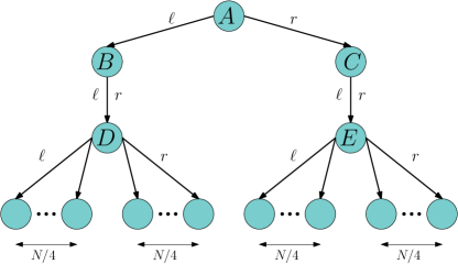
Figure 5: The Widetree domain used in experiments. We have an MDP with $N+5$ states where $N$ of them are terminal states (or leaves.) Each state has two actions $\ell$ and $r$. At states $B$ and $C$, both actions lead to the same state $D$ and $E$ respectively. At states $D$ and $E$, both actions stochastically transition the state to one of $N/4$ terminal states with uniform probability. The true dynamics $M^{\star}$ is shown in the figure. The cost $c(s,a)=\epsilon<<1$ at any $s\neq B$ and $c(B,a)=1$, for any action $a$. Thus, the action taken at $A$ is critical. Model class $\mathcal{M}$ contains only two models: $M^{\mathsf{good}}$ which captures dynamics at $A$ correctly but makes mistakes everywhere else, while $M^{\mathsf{bad}}$ makes mistakes only at $A$ but captures true dynamics everywhere else.

We implement Algorithm 4 using Hedge (Freund & Schapire, 1997) by maintaining a discrete distribution $(p,1-p)$ over the two models $M^{\mathsf{good}}$ and $M^{\mathsf{bad}}$. We use $\epsilon=0.9$ for the hedge update.

C.1.3 Linear Dynamical System

In this experiment, the task is to control a linear dynamical system where the true dynamics are time-varying but the model class only contains time-invariant linear dynamical models. The system has a 5-D state, a 1-D control input, and we are tasked with controlling it for a horizon of $100$ timesteps. The true dynamics evolves according to $x_{t+1}=A_{t}x_{t}+B_{t}u_{t}$ where,

$$A_{t}=\begin{bmatrix}0.5&0\\ 0&0.5\end{bmatrix}$$

when $t$ is even and,

$$A_{t}=\begin{bmatrix}1.5&0\\ 0&1.5\end{bmatrix}$$

when $t$ is odd. The model class $\mathcal{M}$ consists of linear dynamical models of the form $\{x_{t+1}=Ax_{t}+Bu_{t}\}$ and thus cannot model the true dynamics exactly making it an agnostic model class.

The cost function is quadratic as follows,

$$c(\mathbf{x},\mathbf{u})=\sum_{t=0}^{99}u_{t}^{T}u_{t}+x_{100}^{T}x_{100}$$

where $\mathbf{x},\mathbf{u}$ represent the entire state and control trajectory. Note that the cost function only penalizes the control input at every timestep and penalizes the state only at the final timestep.

Given a model $(A,B)\in\mathcal{M}$, we can compute the optimal policy and its value function in closed form by using the finite horizon discrete ricatti solution (Bertsekas, 2005). The value function is represented using matrices $P_{t}\in\mathbb{R}^{5\times 5}$ where $V_{t}(x)=x^{T}P_{t}x$ denotes the cost to go from time $t$ until the end of horizon. Thus, we can construct the loss for any model $M=(A,B)$ in Algorithm 4 for LAMPS-MM as,

$$\ell_{t}(A,B)=\mathop{{}\mathbb{E}}_{(x_{h},u_{h},x_{h+1})\sim\mathcal{D}_{t}}(x_{h+1}^{T}P_{h+1}x_{h+1}-(Ax_{h}+Bu_{h})^{T}P_{h+1}(Ax_{h}+Bu_{h}))^{2}$$

whereas the MLE loss for SysID is simply,

$$\ell_{t}(A,B)=\mathop{{}\mathbb{E}}_{(x_{h},u_{h},x_{h+1})\sim\mathcal{D}_{t}}\|x_{h+1}-(Ax_{h}+Bu_{h})\|_{2}^{2}$$

C.1.4 Maze

Figure 6: The PointMaze (large) environment. Picture taken from https://sites.google.com/view/d4rl/home.

For the maze environment, we adopt the PointMaze (large) task from D4RL (Fu et al., 2020). We present a visualization of the task in Figure 6. While the original offline dataset contains 4000000 samples, we only take 10000 and 50000 samples in our experiment.

C.2 Additional Mujoco Experiment

In this section, we show an additional mujoco experiment. In this case, our algorithm is outperformed by MBPO-SysID initially and reaches the same performance given enough data. We hypothesize that the main cause for this is that the explore distribution does not have high quality in this case, which suggests that Algorithm 3 is more sensitive to the quality of the exploration distribution than MBPO-SysID, as described in Section 5.

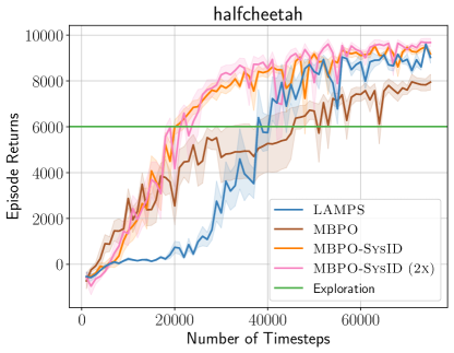
Figure 7: Result on the Halfcheetah benchmark. The results are average over 5 random seeds and the shaded area denotes the standard error. We use 10000 exploration samples. Note that in this case, LAMPS takes more sample to reach the asymptotic performance of MBPO-SysID.

C.3 Implementation Details and Hyperparameters

In this section, we provide the implementation details and hyperparameter we used in our experiments in Section 7.4 and Section 7.5. As mentioned in the main text, our implementation for MBPO is based on Pineda et al. (2021), so does MBPO-SysID and LAMPS. For model training, all baselines use the same ensemble of models as in the original MBPO, while MBPO-SysID and LAMPS use both the data aggregation and exploration data to train the model. For the policy training, MBPO-SysID uses the same branch update as in MBPO with Soft Actor-Critic (SAC), and LAMPS uses a different objective by replacing $Q$-value with the disadvantage term during the actor update step (note that this implies that the actor update is also only based on the exploration distribution.) We present the detailed algorithm in Algorithm 6.

Algorithm 6 Deep LAMPS

0:  Number of iterations $T$, model ensemble $M_{\theta}$, policy $\pi_{\phi}$, value function $q_{\psi}$, exploration dataset $\nu$, policy rollout step $H$, model rollout $E$, model rollout horizon $k$.

1:  Initialize data aggregation $\mathcal{D}=\emptyset$.

2:  for $t=1,\dots,T$ do

3:     Train model ensemble $M_{\theta}$ with MLE with $\rho=\frac{1}{2}\nu+\frac{1}{2}\mathcal{D}$: with $\frac{1}{2}$ probability sampling from $\nu$ and $\frac{1}{2}$ probability sampling from $\mathcal{D}$.

4:     for $h=1,\dots,H$ do

5:        Collect data in $M^{\star}$ by rolling out $\pi_{\phi}$

6:        Initialize model buffer $\mathcal{D}_{model}=\emptyset$.

7:        for $e=1,\dots,E$ do

8:           Sample state $s$ uniformly from $\rho$, rollout $k$ step with $\pi_{\theta}$ and add trajectory to $\mathcal{D}_{model}$

9:           Update soft $Q$-value function $q_{\psi}$ with $\mathcal{D}_{model}$.

10:           Update policy $\pi_{\phi}$ with

$$\mathcal{J}(\pi_{\phi},\nu,q_{\psi})=\mathbb{E}_{s,a\sim\nu}\left[\mathbb{E}_{\tilde{a}\sim\pi_{\phi}(s)}\log(\pi_{\phi}(\tilde{a}\mid s))-(q_{\psi}(s,\tilde{a})-q_{\psi}(s,a))\right]$$

11:        end for

12:     end for

13:  end for

14:  Return Sequence of policies $\{\hat{\pi}_{t}\}_{t=1}^{T+1}$

We use the default hyperparameter for most case, but we present them for completeness. Note that the hyperparameters are the same for all baselines, but MBPO-SysID (2x) uses double the number indicated with the hyperparameter ends with $(\ast)$.

Table 1: Hyperparameters for HalfCheetah

	Value
Exploration sample size	10000
Ensemble size	7
Ensemble elite number	5
Model learning rate	0.001
Model batch size	256
Rollout step in learned model ($\ast$)	400
Rollout length	$1\to 1$
Number policy updates ($\ast$)	20
Policy type	Stochastic Gaussian Policy

Table 2: Hyperparameters for Ant

	Value
Exploration sample size	10000
Ensemble size	7
Ensemble elite number	5
Model learning rate	0.0003
Model batch size	256
Rollout step in learned model ($\ast$)	400
Rollout length	$1\to 25$
Number policy updates ($\ast$)	20
Policy type	Stochastic Gaussian Policy

Table 3: Hyperparameters for Hopper

	Value
Exploration sample size	10000
Ensemble size	7
Ensemble elite number	5
Model learning rate	0.001
Model batch size	256
Rollout step in learned model ($\ast$)	400
Rollout length	$1\to 15$
Number policy updates ($\ast$)	40
Policy type	Stochastic Gaussian Policy

Table 4: Hyperparameters for Humanoid

	Value
Exploration sample size	10000
Ensemble size	7
Ensemble elite number	5
Model learning rate	0.0003
Model batch size	256
Rollout step in learned model ($\ast$)	400
Rollout length	$1\to 25$
Number policy updates ($\ast$)	20
Policy type	Stochastic Gaussian Policy

Table 5: Hyperparameters for Walker

	Value
Exploration sample size	10000
Ensemble size	7
Ensemble elite number	5
Model learning rate	0.001
Model batch size	256
Rollout step in learned model ($\ast$)	400
Rollout length	$1\to 1$
Number policy updates ($\ast$)	20
Policy type	Stochastic Gaussian Policy

Table 6: Hyperparameters for PointMaze

	Value
Exploration sample size	10000/50000
Ensemble size	7
Ensemble elite number	5
Model learning rate	0.001
Model batch size	256
Rollout step in learned model ($\ast$)	400
Rollout length	$1\to 1$
Number policy updates ($\ast$)	20
Policy type	Deterministic Policy

References

- Abbasi-Yadkori & Szepesvári (2011) Abbasi-Yadkori, Y. and Szepesvári, C. Regret bounds for the adaptive control of linear quadratic systems. In Proceedings of the 24th Annual Conference on Learning Theory, pp. 1–26. JMLR Workshop and Conference Proceedings, 2011.
- Abbeel & Ng (2005) Abbeel, P. and Ng, A. Y. Exploration and apprenticeship learning in reinforcement learning. In Raedt, L. D. and Wrobel, S. (eds.), Machine Learning, Proceedings of the Twenty-Second International Conference (ICML 2005), Bonn, Germany, August 7-11, 2005, volume 119 of ACM International Conference Proceeding Series, pp. 1–8. ACM, 2005. doi: 10.1145/1102351.1102352. URL https://doi.org/10.1145/1102351.1102352.
- Ayoub et al. (2020) Ayoub, A., Jia, Z., Szepesvari, C., Wang, M., and Yang, L. Model-based reinforcement learning with value-targeted regression. In International Conference on Machine Learning, pp. 463–474. PMLR, 2020.
- Azar et al. (2013) Azar, M. G., Munos, R., and Kappen, H. J. Minimax pac bounds on the sample complexity of reinforcement learning with a generative model. Machine learning, 91(3):325–349, 2013.
- Bagnell et al. (2003) Bagnell, J. A., Kakade, S. M., Ng, A. Y., and Schneider, J. G. Policy search by dynamic programming. In Thrun, S., Saul, L. K., and Schölkopf, B. (eds.), Advances in Neural Information Processing Systems 16 [Neural Information Processing Systems, NIPS 2003, December 8-13, 2003, Vancouver and Whistler, British Columbia, Canada], pp. 831–838. MIT Press, 2003. URL https://proceedings.neurips.cc/paper/2003/hash/3837a451cd0abc5ce4069304c5442c87-Abstract.html.
- Bertsekas (2005) Bertsekas, D. P. Dynamic programming and optimal control, 3rd Edition. Athena Scientific, 2005. ISBN 1886529264. URL https://www.worldcat.org/oclc/314894080.
- Brockman et al. (2016) Brockman, G., Cheung, V., Pettersson, L., Schneider, J., Schulman, J., Tang, J., and Zaremba, W. Openai gym. arXiv preprint arXiv:1606.01540, 2016.
- Cesa-Bianchi et al. (2004) Cesa-Bianchi, N., Conconi, A., and Gentile, C. On the generalization ability of on-line learning algorithms. IEEE Transactions on Information Theory, 50(9):2050–2057, 2004.
- Chua et al. (2018) Chua, K., Calandra, R., McAllister, R., and Levine, S. Deep reinforcement learning in a handful of trials using probabilistic dynamics models. In Advances in Neural Information Processing Systems, pp. 4754–4765, 2018.
- Eysenbach et al. (2021) Eysenbach, B., Khazatsky, A., Levine, S., and Salakhutdinov, R. Mismatched no more: Joint model-policy optimization for model-based rl. arXiv preprint arXiv:2110.02758, 2021.
- Farahmand et al. (2017) Farahmand, A. M., Barreto, A., and Nikovski, D. Value-aware loss function for model-based reinforcement learning. In Singh, A. and Zhu, X. J. (eds.), Proceedings of the 20th International Conference on Artificial Intelligence and Statistics, AISTATS 2017, 20-22 April 2017, Fort Lauderdale, FL, USA, volume 54 of Proceedings of Machine Learning Research, pp. 1486–1494. PMLR, 2017. URL http://proceedings.mlr.press/v54/farahmand17a.html.
- Freund & Schapire (1997) Freund, Y. and Schapire, R. E. A decision-theoretic generalization of on-line learning and an application to boosting. J. Comput. Syst. Sci., 55(1):119–139, 1997. doi: 10.1006/jcss.1997.1504. URL https://doi.org/10.1006/jcss.1997.1504.
- Fu et al. (2020) Fu, J., Kumar, A., Nachum, O., Tucker, G., and Levine, S. D4rl: Datasets for deep data-driven reinforcement learning. arXiv preprint arXiv:2004.07219, 2020.
- Grimm et al. (2020) Grimm, C., Barreto, A., Singh, S., and Silver, D. The value equivalence principle for model-based reinforcement learning. Advances in Neural Information Processing Systems, 33:5541–5552, 2020.
- Hafner et al. (2020) Hafner, D., Lillicrap, T., Norouzi, M., and Ba, J. Mastering atari with discrete world models. arXiv preprint arXiv:2010.02193, 2020.
- Hafner et al. (2023) Hafner, D., Pasukonis, J., Ba, J., and Lillicrap, T. Mastering diverse domains through world models. arXiv preprint arXiv:2301.04104, 2023.
- Hazan (2019) Hazan, E. Introduction to online convex optimization. CoRR, abs/1909.05207, 2019. URL http://arxiv.org/abs/1909.05207.
- Hester et al. (2018) Hester, T., Vecerik, M., Pietquin, O., Lanctot, M., Schaul, T., Piot, B., Horgan, D., Quan, J., Sendonaris, A., Osband, I., et al. Deep q-learning from demonstrations. In Proceedings of the AAAI Conference on Artificial Intelligence, volume 32, 2018.
- Janner et al. (2019) Janner, M., Fu, J., Zhang, M., and Levine, S. When to trust your model: Model-based policy optimization. Advances in Neural Information Processing Systems, 32, 2019.
- Jiang (2018) Jiang, N. PAC reinforcement learning with an imperfect model. In McIlraith, S. A. and Weinberger, K. Q. (eds.), Proceedings of the Thirty-Second AAAI Conference on Artificial Intelligence, (AAAI-18), the 30th innovative Applications of Artificial Intelligence (IAAI-18), and the 8th AAAI Symposium on Educational Advances in Artificial Intelligence (EAAI-18), New Orleans, Louisiana, USA, February 2-7, 2018, pp. 3334–3341. AAAI Press, 2018. URL https://www.aaai.org/ocs/index.php/AAAI/AAAI18/paper/view/16052.
- Joseph et al. (2013) Joseph, J. M., Geramifard, A., Roberts, J. W., How, J. P., and Roy, N. Reinforcement learning with misspecified model classes. In 2013 IEEE International Conference on Robotics and Automation, Karlsruhe, Germany, May 6-10, 2013, pp. 939–946. IEEE, 2013. doi: 10.1109/ICRA.2013.6630686. URL https://doi.org/10.1109/ICRA.2013.6630686.
- Kakade et al. (2020) Kakade, S., Krishnamurthy, A., Lowrey, K., Ohnishi, M., and Sun, W. Information theoretic regret bounds for online nonlinear control. Advances in Neural Information Processing Systems, 33:15312–15325, 2020.
- Kakade (2003) Kakade, S. M. On the sample complexity of reinforcement learning. University of London, University College London (United Kingdom), 2003.
- Kakade & Langford (2002) Kakade, S. M. and Langford, J. Approximately optimal approximate reinforcement learning. In Sammut, C. and Hoffmann, A. G. (eds.), Machine Learning, Proceedings of the Nineteenth International Conference (ICML 2002), University of New South Wales, Sydney, Australia, July 8-12, 2002, pp. 267–274. Morgan Kaufmann, 2002.
- Kearns & Singh (2002) Kearns, M. and Singh, S. Near-optimal reinforcement learning in polynomial time. Machine learning, 49(2):209–232, 2002.
- Kearns et al. (1999) Kearns, M. J., Mansour, Y., and Ng, A. Y. Approximate planning in large pomdps via reusable trajectories. In Solla, S. A., Leen, T. K., and Müller, K. (eds.), Advances in Neural Information Processing Systems 12, [NIPS Conference, Denver, Colorado, USA, November 29 - December 4, 1999], pp. 1001–1007. The MIT Press, 1999. URL http://papers.nips.cc/paper/1664-approximate-planning-in-large-pomdps-via-reusable-trajectories.
- Lambert et al. (2020) Lambert, N. O., Amos, B., Yadan, O., and Calandra, R. Objective mismatch in model-based reinforcement learning. In Bayen, A. M., Jadbabaie, A., Pappas, G. J., Parrilo, P. A., Recht, B., Tomlin, C. J., and Zeilinger, M. N. (eds.), Proceedings of the 2nd Annual Conference on Learning for Dynamics and Control, L4DC 2020, Online Event, Berkeley, CA, USA, 11-12 June 2020, volume 120 of Proceedings of Machine Learning Research, pp. 761–770. PMLR, 2020. URL http://proceedings.mlr.press/v120/lambert20a.html.
- Levine & Abbeel (2014) Levine, S. and Abbeel, P. Learning neural network policies with guided policy search under unknown dynamics. Advances in neural information processing systems, 27, 2014.
- Li & Todorov (2004) Li, W. and Todorov, E. Iterative linear quadratic regulator design for nonlinear biological movement systems. In Araújo, H., Vieira, A., Braz, J., Encarnação, B., and Carvalho, M. (eds.), ICINCO 2004, Proceedings of the First International Conference on Informatics in Control, Automation and Robotics, Setúbal, Portugal, August 25-28, 2004, pp. 222–229. INSTICC Press, 2004.
- Ljung (1998) Ljung, L. System identification. In Signal analysis and prediction, pp. 163–173. Springer, 1998.
- Modhe et al. (2021) Modhe, N., Kamath, H., Batra, D., and Kalyan, A. Model-advantage optimization for model-based reinforcement learning. arXiv preprint arXiv:2106.14080, 2021.
- Morari & Lee (1999) Morari, M. and Lee, J. H. Model predictive control: past, present and future. Computers & Chemical Engineering, 23(4-5):667–682, 1999.
- Nair et al. (2018) Nair, A., McGrew, B., Andrychowicz, M., Zaremba, W., and Abbeel, P. Overcoming exploration in reinforcement learning with demonstrations. In 2018 IEEE international conference on robotics and automation (ICRA), pp. 6292–6299. IEEE, 2018.
- Pineda et al. (2021) Pineda, L., Amos, B., Zhang, A., Lambert, N. O., and Calandra, R. Mbrl-lib: A modular library for model-based reinforcement learning. arXiv preprint arXiv:2104.10159, 2021.
- Rajeswaran et al. (2017) Rajeswaran, A., Kumar, V., Gupta, A., Vezzani, G., Schulman, J., Todorov, E., and Levine, S. Learning complex dexterous manipulation with deep reinforcement learning and demonstrations. arXiv preprint arXiv:1709.10087, 2017.
- Ross & Bagnell (2012) Ross, S. and Bagnell, J. A. Agnostic system identification for model-based reinforcement learning. In Proceedings of the 29th International Coference on International Conference on Machine Learning, pp. 1905–1912, 2012.
- Ross & Bagnell (2014) Ross, S. and Bagnell, J. A. Reinforcement and imitation learning via interactive no-regret learning. CoRR, abs/1406.5979, 2014. URL http://arxiv.org/abs/1406.5979.
- Schrittwieser et al. (2020) Schrittwieser, J., Antonoglou, I., Hubert, T., Simonyan, K., Sifre, L., Schmitt, S., Guez, A., Lockhart, E., Hassabis, D., Graepel, T., et al. Mastering atari, go, chess and shogi by planning with a learned model. Nature, 588(7839):604–609, 2020.
- Song & Sun (2021) Song, Y. and Sun, W. Pc-mlp: Model-based reinforcement learning with policy cover guided exploration. In International Conference on Machine Learning, pp. 9801–9811. PMLR, 2021.
- Song et al. (2022) Song, Y., Zhou, Y., Sekhari, A., Bagnell, J. A., Krishnamurthy, A., and Sun, W. Hybrid rl: Using both offline and online data can make rl efficient. arXiv preprint arXiv:2210.06718, 2022.
- Sun et al. (2019a) Sun, W., Jiang, N., Krishnamurthy, A., Agarwal, A., and Langford, J. Model-based rl in contextual decision processes: Pac bounds and exponential improvements over model-free approaches. In Conference on learning theory, pp. 2898–2933. PMLR, 2019a.
- Sun et al. (2019b) Sun, W., Vemula, A., Boots, B., and Bagnell, D. Provably efficient imitation learning from observation alone. In Chaudhuri, K. and Salakhutdinov, R. (eds.), Proceedings of the 36th International Conference on Machine Learning, ICML 2019, 9-15 June 2019, Long Beach, California, USA, volume 97 of Proceedings of Machine Learning Research, pp. 6036–6045. PMLR, 2019b. URL http://proceedings.mlr.press/v97/sun19b.html.
- Sutton (1991) Sutton, R. S. Dyna, an integrated architecture for learning, planning, and reacting. ACM Sigart Bulletin, 2(4):160–163, 1991.
- Sutton & Barto (2018) Sutton, R. S. and Barto, A. G. Reinforcement learning: An introduction. MIT press, 2018.
- Swamy et al. (2021) Swamy, G., Choudhury, S., Bagnell, J. A., and Wu, S. Of moments and matching: A game-theoretic framework for closing the imitation gap. In International Conference on Machine Learning, pp. 10022–10032. PMLR, 2021.
- Tu & Recht (2019) Tu, S. and Recht, B. The gap between model-based and model-free methods on the linear quadratic regulator: An asymptotic viewpoint. In Conference on Learning Theory, pp. 3036–3083. PMLR, 2019.
- Vecerik et al. (2017) Vecerik, M., Hester, T., Scholz, J., Wang, F., Pietquin, O., Piot, B., Heess, N., Rothörl, T., Lampe, T., and Riedmiller, M. Leveraging demonstrations for deep reinforcement learning on robotics problems with sparse rewards. arXiv preprint arXiv:1707.08817, 2017.
- Vemula et al. (2020) Vemula, A., Oza, Y., Bagnell, J. A., and Likhachev, M. Planning and execution using inaccurate models with provable guarantees. In Toussaint, M., Bicchi, A., and Hermans, T. (eds.), Robotics: Science and Systems XVI, Virtual Event / Corvalis, Oregon, USA, July 12-16, 2020, 2020. doi: 10.15607/RSS.2020.XVI.001. URL https://doi.org/10.15607/RSS.2020.XVI.001.
- Voloshin et al. (2021) Voloshin, C., Jiang, N., and Yue, Y. Minimax model learning. In International Conference on Artificial Intelligence and Statistics, pp. 1612–1620. PMLR, 2021.
- Wu et al. (2022) Wu, P., Escontrela, A., Hafner, D., Goldberg, K., and Abbeel, P. Daydreamer: World models for physical robot learning. arXiv preprint arXiv:2206.14176, 2022.
- Xie et al. (2021a) Xie, T., Cheng, C.-A., Jiang, N., Mineiro, P., and Agarwal, A. Bellman-consistent pessimism for offline reinforcement learning. Advances in neural information processing systems, 34:6683–6694, 2021a.
- Xie et al. (2021b) Xie, T., Jiang, N., Wang, H., Xiong, C., and Bai, Y. Policy finetuning: Bridging sample-efficient offline and online reinforcement learning. Advances in neural information processing systems, 34:27395–27407, 2021b.