Contact process with aperiodic temporal disorder

Abstract

We investigate the nonequilibrium critical behavior of the contact process with deterministic aperiodic temporal disorder implemented by choosing healing or infection rates according to a family of aperiodic sequences based on the quasiperiodic Fibonacci sequence. This family allows us to gauge the temporal fluctuations via a wandering exponent $\omega$ and put our work in the context of the Kinzel–Vojta–Dickman criterion for the relevance of temporal disorder to the critical behavior of nonequilibrium models. By means of analytic and numerical calculations, the generalized criterion is tested in the mean-field limit.

I Introduction

Nonequilibrium phase transitions (Marro and Dickman, 2006) offer an interesting extension of ideas developed in the context of equilibrium critical phenomena to problems in which time plays a central role. This is the case of problems featuring absorbing states (Hinrichsen, 2000), such as turbulence in liquid crystals (Takeuchi et al., 2007), reaction-diffusion processes (Alcaraz et al., 1994), and extinction phenomena in biology (Murray, 2007).

A paradigmatic model for these problems is the contact process (Harris, 1974a), which can be formulated as describing the dynamics of an epidemics. The model assumes that individuals fixed at the vertices of a fully occupied lattice can be either infected or healed. Infected individuals transmit the infection to its nearest neighbors at a rate $\lambda$, and become healed at a rate $\mu$. It is now well established that, for a fixed healing rate $\mu$, there is a critical value $\lambda_{c}$ of the infection rate $\lambda$ separating and active phase ($\lambda>\lambda_{c}$), in which the epidemics persists indefinitely, from an inactive (absorbing) phase ($\lambda<\lambda_{c}$), in which the epidemics stops after a finite time (see, e.g., Refs. Marro and Dickman, 2006; Tomé and Oliveira, 2015 and references therein).

Remarkably, concepts of equilibrium phase transitions, such as scaling invariance and universality class, are quite useful to describe the non-analyticity of this nonequilibrium phase transition. This is because fluctuations of the order parameter field (the density of infected individuals $\rho$) are self similar at the transition. This means that the length $\xi$ and time $\xi_{t}$ scales of this fluctuations diverge when approaching the critical point. More precisely,

$$\xi_{t}\left(\epsilon\right)\sim\left|\epsilon\right|^{-\nu_{\parallel}},$$ (1)

where $\epsilon=\lambda_{c}-\lambda$ is the distance from criticality, and $\nu_{\parallel}$ is the correlation-time critical exponent. Likewise, $\xi\sim\left|\epsilon\right|^{-\nu_{\perp}}$. The other critical exponents of interest to our work are the order-parameter exponent $\beta$, which is defined from

$$\rho\left(\epsilon\right)\sim\left(-\epsilon\right)^{\beta},$$ (2)

and $\delta$ (Faria et al., 2008; Barghathi et al., 2014), the critical exponent defining the power-law relaxation of the density at the critical point,

$$\rho_{c}\left(t\right)\sim t^{-\delta}.$$ (3)

In general, we expect $\xi_{t}$ to be related to the time needed for the asymptotic behavior to set in, so that $\rho\left(\epsilon\right)\sim\xi_{t}^{-\beta/\nu_{\parallel}}\sim\rho_{c}\left(\xi_{t}\right),$ and we conclude that

$$\delta=\frac{\beta}{\nu_{\parallel}}.$$ (4)

In the mean-field limit, we have $\nu_{\parallel}=\beta=\delta=1$. In 1D, these exponents are $\nu_{\parallel}\approx 1.73$, $\beta\approx 0.28$, and $\delta\approx 0.16$ (Ódor, 2004).

As in equilibrium, disorder may also have profound effects in nonequilibrium phase transitions, with the additional aspect that disorder ingredients may be present over space as well as over time. In ecological models, for instance, spatial disorder represents the variation of environmental conditions across the terrain, whereas temporal disorder represents fluctuations in environmental conditions over time.

In the contact process, disorder can be implemented by allowing the rates $\lambda$ and $\mu$ to vary over the sites of the lattice or over time. The contact process with spatial disorder has been extensively studied (see, e.g., Refs. Noest, 1986; Hooyberghs et al., 2003; Vojta and Dickison, 2005; Vojta and Lee, 2006; Hoyos, 2008; Faria et al., 2008; Barghathi et al., 2014), and only recently the effects of temporal disorder has attracted attention (Vazquez et al., 2011; Vojta and Hoyos, 2015; Barghathi et al., 2016; de Oliveira and Fiore, 2016; Solano et al., 2016; Wada et al., 2018; Fiore et al., 2018; Encinas and Fiore, 2021; Wada and Hoyos, 2021).

Prominent among the latter investigations are Refs. Vojta and Hoyos, 2015; Barghathi et al., 2016; Wada et al., 2018, which explore how the critical behavior of the contact process is affected by random temporal disorder, both uncorrelated (Vojta and Hoyos, 2015; Barghathi et al., 2016) and correlated (Wada et al., 2018) disorder. These works show that the introduction of temporal disorder induces an infinite-noise critical point, in which density fluctuations increase without limit with time. As a result, the ensemble typical and arithmetic averages of the population density behave quite differently. As time increases, the former becomes much less than the latter (which is dominated by rare events).

Disorder is introduced in the model in the following way: we consider consecutive time intervals of same duration $\Delta t_{n}$. To the $n$th time interval, we assign an infection $\lambda_{n}$ and healing $\mu_{n}$ rate which are uniform throughout the lattice. In the random case, the parameters $\left(\lambda_{n},\mu_{n}\right)$ are chosen from a probability distribution. Here, in the aperiodic case, $\left(\lambda_{n},\mu_{n}\right)=\left(\lambda_{A},\mu_{A}\right)$ or $\left(\lambda_{B},\mu_{B}\right)$ depending on whether the $n$th letter of a word $A$ or $B$. This word is obtained employing the generalized Fibonacci sequence. Starting with the letter $A$, we apply the inflation rules $A\rightarrow AB^{k}$ and $B\rightarrow A$, where $B^{k}$ denotes $k$ consecutive letters $B$. For $k=1$, we recover the original Fibonacci sequence.

Although deterministic, the iterated sequence has no period and is characterized by intrinsic temporal fluctuations growing as $\sim t^{\omega}$, with the so-called wandering exponent $\omega$ dependent on the value of $k$.

In close analogy with Luck’s (Luck, 1993) generalization of the Harris criterion (Harris, 1974b) for the relevance of spatial disorder on phase transitions in thermodynamic equilibrium, it is possible to derive a perturbative criterion for the relevance of aperiodic temporal disorder on the nonequilibrium case. Near criticality ($\left|\epsilon\right|\ll 1$) and along the characteristic time scale $\xi_{t}$, fluctuations of $\epsilon$ are of order $\xi_{t}^{\omega}$ [see Eq. (47) in Appendix A], so that the corresponding average fluctuations are

$$\delta\epsilon\sim\frac{\xi_{t}^{\omega}}{\xi_{t}}\sim\left|\epsilon\right|^{\left(1-\omega\right)\nu_{\parallel}}.$$ (5)

Aperiodic temporal disorder is a relevant perturbation to the clean critical theory if $\delta\epsilon\gg\left|\epsilon\right|$, which, thus, leads to the criterion

$$\left(1-\omega\right)\nu_{\parallel}<1.$$ (6)

Notice that for uncorrelated random temporal disorder we have $\omega=\frac{1}{2}$ and the inequality (6) reduces to the temporal version of the Harris–Luck criterion, $\nu_{\parallel}<2$, formulated by Kinzel (Kinzel, 1985) and by Vojta and Dickman (Vojta and Dickman, 2016). In fact, these last authors also investigated the case of correlated random temporal disorder characterized by a power-law correlations with an exponent $\gamma$, finding out that in this case the criterion for instability of the critical behavior in the presence of disorder becomes $\gamma\nu_{\parallel}<2$. As $\gamma$ is related to the Hurst exponent by $\gamma=2-2H$ (Wada et al., 2018), the criterion can also be written as $\left(1-H\right)\nu_{\parallel}<1$. Comparing with Eq. (6), we see that, for deterministic aperiodic temporal disorder, the wandering exponent $\omega$ plays the role that the Hurst exponent plays for random correlated temporal disorder.

In this paper, our aim is to test the stability criterion (6) in the mean-field limit of the contact process, which allows for extensive analytical work to be performed, enabling us to obtain results for the long-time behavior and the critical exponents of the model. In Section II, we sketch the mean-field treatment, writing a recurrence equation for the density of infected agents at the beginning of each time interval and analytically determining the criticality condition. In Section III, we describe a renormalization-group (RG) treatment that allows us to present analytical results for some critical exponents, which turn out to depend on $k$. Numerical calculations needed to extract further information are described in Section IV. There are also two appendices, describing some technical details.

II Mean-Field limit

(a)

(b)

(c)

Figure 1: (a) Plot of $\rho_{n}=\rho\left(t_{n}\right)$ vs. $n$ (with $t_{n}=n$$\Delta t$) for $k=2$ and $\lambda_{A}<\mu<\lambda_{B}$. (b) Implementing the RG treatment of the dynamics, which consists in grouping all consecutive time intervals with the same $r_{n}$. (c) As a result of the grouping, the effective system has parameters $\tilde{r}$ and $\tilde{\Delta t}$.

In this Section we consider the mean-field limit of the contact process with aperiodic temporal disorder. As $\nu_{\parallel}=1$ in mean-field, the generalized Harris criterion (6) says that aperiodic temporal disorder is a relevant perturbation when $\omega>\omega^{*}=0$. As shown in Appendix A, $\omega_{k=1}<\omega_{c}$, $\omega_{k=2}=\omega_{c}$, and $\omega_{k>2}>\omega_{c}$. Thus, changing $k$ from $1$ to $3$ gives us the rare opportunity to test the criterion (6) in all possible situations (irrelevant, marginal, and relevant) by analytical means.

During the time interval between $t_{n-1}$ and $t_{n}=t_{n-1}+\Delta t_{n}$, the density of active sites can be described by the logistic equation (Marro and Dickman, 2006; Tomé and Oliveira, 2015; Vojta and Hoyos, 2015; Barghathi et al., 2016)

$$\frac{d\rho}{dt}=\left(\lambda_{n}-\mu_{n}\right)\rho-\lambda_{n}\rho^{2},$$ (7)

in which $\lambda_{n}$ and $\mu_{n}$ are respectively the infection and healing rates during that time interval, which lasts a time $\Delta t_{n}$. It is immediate to integrate Eq. (7) to obtain, for $t_{n-1}\leq t\leq t_{n}$,

$$\frac{1}{\rho\left(t\right)}=\frac{e^{\left(\mu_{n}-\lambda_{n}\right)\left(t-t_{n-1}\right)}}{\rho_{n-1}}+\frac{\lambda_{n}\left[e^{\left(\mu_{n}-\lambda_{n}\right)\left(t-t_{n-1}\right)}-1\right]}{\mu_{n}-\lambda_{n}},$$ (8)

with the notation $\rho_{n}\equiv\rho\left(t_{n}\right)$. Imposing continuity of $\rho\left(t\right)$ at $t=t_{n}$ leads to the recursion relation

$$\rho_{n}^{-1}=r_{n}\rho_{n-1}^{-1}+s_{n},$$ (9)

with

$$r_{n}=e^{\left(\mu_{n}-\lambda_{n}\right)\Delta t_{n}}\quad\text{and}\quad s_{n}=\frac{r_{n}-1}{\mu_{n}-\lambda_{n}}\lambda_{n}.$$ (10)

Notice that for $\mu_{n}>\lambda_{n}$ we have $r_{n}>1$, while for $\mu_{n}<\lambda_{n}$ we have $0<r_{n}<1$; as for $s_{n}$, it is always non-negative. Thus, as expected, $\rho_{n}$ decreases when $\mu_{n}>\lambda_{n}$ and increase only when $\mu_{n}<\lambda_{n}$, as illustrated in Fig. 1a.

Iterating the recursion relation in Eq. (9) yields $\rho_{n}^{-1}=R_{n}\rho_{0}^{-1}+S_{n},$in which

$$R_{n}=\prod_{i=1}^{n}r_{i}\quad\text{and}\quad S_{n}=s_{n}+\sum_{i=1}^{n-1}s_{i}\prod_{j=i+1}^{n}r_{j}.$$ (11)

The term $S_{n}$ is responsible for preventing $\rho_{n}$ from becoming greater than $1$. On the other hand, the fate of the infection when $\rho_{n}\ll 1$ lies essentially on the term $R_{n}$, which, defining

$$\left\langle\lambda\right\rangle_{n}=\frac{1}{t_{n}}\sum_{i=1}^{n}\lambda_{i}\Delta t_{i}\quad\text{and}\quad\left\langle\mu\right\rangle_{n}=\frac{1}{t_{n}}\sum_{i=1}^{n}\mu_{i}\Delta t_{i},$$ (12)

can be written as

$$R_{n}=e^{\left(\left\langle\mu\right\rangle_{n}-\left\langle\lambda\right\rangle_{n}\right)t_{n}}.$$ (13)

Clearly, we have two different regimes as $n\rightarrow\infty$. If $\left\langle\mu\right\rangle_{n}>\left\langle\lambda\right\rangle_{n}$, then $R_{n}$ grows without limit and $\rho_{n}$ approaches zero, indicating an inactive phase. On the other hand, if $\left\langle\mu\right\rangle_{n}<\left\langle\lambda\right\rangle_{n}$, then $R_{n}$ approaches zero and $\rho_{n}$ remains finite, indicating an active phase. Thus, the limiting case $\left\langle\mu\right\rangle_{n}=\left\langle\lambda\right\rangle_{n}$ signals the critical point. The behavior of the system exactly at the critical point is governed by the fluctuations in the rates $\lambda_{n}$ and $\mu_{n}$, which depend on the precise way in which they are chosen.

For simplicity and without loss of generality, from now on we assume a constant duration of each time interval, $\Delta t_{n}\equiv\Delta t$, and set $\mu_{A}=\mu_{B}=\mu$. Thus, $\left\langle\mu\right\rangle_{n}=\mu$ and

$$\left\langle\lambda\right\rangle_{N}=\frac{1}{N}\sum_{i=1}^{N}\lambda_{i}=\frac{N_{A}}{N}\lambda_{A}+\frac{N_{B}}{N}\lambda_{B},$$ (14)

in which $N_{A}$ and $N_{B}$ are the numbers of letters $A$ and $B$ in the generalized Fibonacci sequence of length $N$. The fraction of letters in the infinite word (see Appendix A) are

$$x_{A}\equiv\lim_{N\rightarrow\infty}\frac{N_{A}}{N}=\zeta_{+}^{-1},$$

and $x_{B}\equiv 1-x_{A}$, with

$$\zeta_{\pm}=\frac{1\pm\sqrt{1+4k}}{2}.$$ (15)

The critical point $\lim_{N\rightarrow\infty}\left\langle\lambda\right\rangle_{N}=\lim_{N\rightarrow\infty}\left\langle\mu\right\rangle_{N}$ can, therefore, be recast as

$$x_{A}\lambda_{A}+x_{B}\lambda_{B}=\mu.$$ (16)

Assuming $\lambda_{A}<\lambda_{B}$, it is clear from Eq. (16) that at the critical point we must have $\lambda_{A}<\mu<\lambda_{B}$. Thus, sufficiently close to the critical point, $\rho\left(t\right)$ will decrease or increase during the $n$th time interval depending on whether $\lambda_{n}=\lambda_{A}$ or $\lambda_{n}=\lambda_{B}$. A plot of $\rho_{n}$ vs $n$ has the form illustrated in Fig. 1a for $k=2$. The regions in which $\rho$ increases have a duration equal to $k$ time intervals, while the regions in which $\rho$ decreases last either $1$ or $k+1$ time intervals.

III RG treatment

We are interested in describing the asymptotic behavior close to the critical point. Since $\rho\left(t\right)\ll 1$ in that case, then we can disregard the term $s_{n}$ in Eq. (9). This is very helpful because only the knowledge of $\left\{r_{n}\right\}$ determines completely the critical behavior of the system. In log-variables, Eq. (9) become an “aperiodic” walk (instead of a random walk) where the steps of the walker is $\ln r_{n}$. Our task now is to determine the properties of this walker.

It is convenient to group consecutive intervals having the same parameters $\left\{\lambda_{n}\right\}=\lambda$ into a single interval with that parameter $\lambda$ and larger duration as depicted in Fig. 1. Therefore, instead of considering $r_{n}$ equal to $r_{B}=e^{\left(\mu-\lambda_{B}\right)\Delta t}$ or $r_{A}=e^{\left(\mu-\lambda_{A}\right)\Delta t}$ in Eq. (9), we need to deal with $r_{n}$ being equal to $r_{0}^{+}=r_{B}^{k}$, $r_{0}^{-}=r_{A}$, and $r_{0}^{--}=r_{A}^{k+1}$. This is because intervals in which $\lambda_{n}=\lambda_{B}$ only appear in a sequence of $k$ $B$-intervals in a row. On the other hand, the $A$-intervals either appear as a single one, or in a sequence of $k+1$ intervals in a row. In addition, we have to consider non-uniform time intervals $\Delta t_{0}^{+}=k\Delta t$, $\Delta t_{0}^{-}=\Delta t$, and $\Delta t_{0}^{++}=\left(k+1\right)\Delta t$, respectively.

In sum, each effective time interval in the regrouped system is characterized by a pair of effective parameters $\left(\tilde{r},\tilde{\Delta t}\right)$ given by $\left(r_{0}^{++},\Delta t_{0}^{++}\right)$, $\left(r_{0}^{-},\Delta t_{0}^{-}\right)$, or $\left(r_{0}^{--},\Delta t_{0}^{--}\right)$ as shown in Fig. 1c. As explicitly shown in Fig. 2a, there are three types ($A$, $B$, and $C$) of intervals to consider.

The reason of the superscripts “$\pm$” is because we are assuming that $\lambda_{A}<\mu<\lambda_{B}$, so that $+$ ($-$) means an interval in which $\rho$ increases (decreases): $r_{0}^{++}<1<r_{0}^{-}<r_{0}^{--}.$ The reason for the subscript “0” is to call attention that these are the bare values. As will become clear below, renormalized values acquire a subscript $j$ denoting the number of times it was renormalized.

(a)

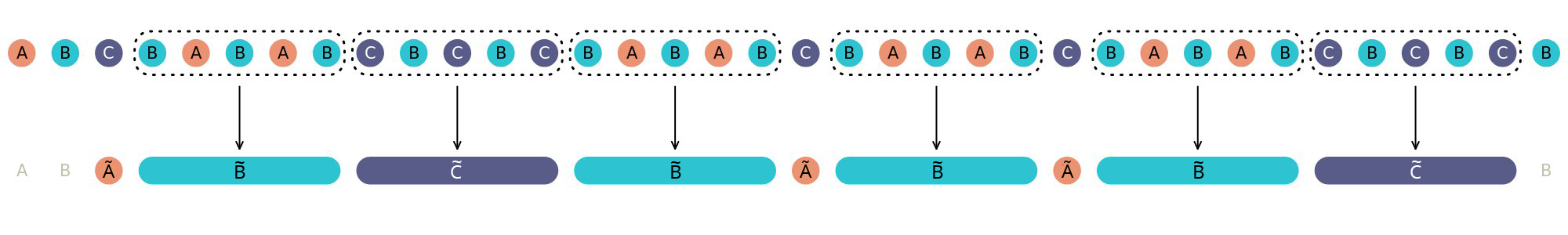
(b)

Figure 2: Pictorial representation of the RG scheme for $k=2$. (a) The initial grouping stage gives rise to three types of effective time intervals, labeled $A$, $B$ and $C$ and characterized by different effective parameters (see main text). The density of active/infected sites increases in $B$-type intervals and decreases in $A$- and $C$-type intervals. (b) Apart from boundary defects, effective intervals generated in the next stage, labeled by $\tilde{A}$, $\tilde{B}$ and $\tilde{C}$, follow the same sequence as the time intervals $A$, $B$ and $C$.

Following Ref. Vojta and Hoyos, 2015, we now formulate an RG treatment to iteratively determine the set of effective parameters $\tilde{r}$ and $\tilde{\Delta t}$ describing the long-time behavior of $\rho\left(t\right)\ll 1$. In the initial stage of the RG treatment, this set corresponds to $\left\{\left(r_{0}^{++},\Delta t_{0}^{++}\right),\left(r_{0}^{-},\Delta t_{0}^{-}\right),\left(r_{0}^{--},\Delta t_{0}^{--}\right)\right\}$. At any given stage, we identify the effective parameter $\ln\tilde{r}$ closest to $0$, which characterizes those effective time intervals during which the density varies the least, and use Eq. (9) to eliminate all those time intervals, generating a new configuration of effective time intervals and defining a new stage of the RG scheme, see Fig. 2b. Importantly, as we checked numerically, in each stage $j$ of this decimation procedure the temporal sequence of effective time intervals is always the same (except for minor boundary effects). Precisely, the effective parameters in the $j$th stage are

$$\left(\begin{array}[]{c}\ln r_{j}^{++}\\ \ln r_{j}^{-}\\ \ln r_{j}^{--}\end{array}\right)=\mathbf{M}\left(\begin{array}[]{c}\ln r_{j-1}^{++}\\ \ln r_{j-1}^{-}\\ \ln r_{j-1}^{--}\end{array}\right)=\mathbf{M}^{j}\left(\begin{array}[]{c}\ln r_{0}^{++}\\ \ln r_{0}^{-}\\ \ln r_{0}^{--}\end{array}\right),$$ (17)

$$\left(\begin{array}[]{c}\Delta t_{j}^{++}\\ \Delta t_{j}^{-}\\ \Delta t_{j}^{--}\end{array}\right)=\mathbf{M}\left(\begin{array}[]{c}\Delta t_{j-1}^{++}\\ \Delta t_{j-1}^{-}\\ \Delta t_{j-1}^{--}\end{array}\right)=\mathbf{M}^{j}\left(\begin{array}[]{c}\ln r_{0}^{++}\\ \ln r_{0}^{-}\\ \ln r_{0}^{--}\end{array}\right),$$ (18)

with

$$\mathbf{M}=\left(\begin{array}[]{ccc}k+1&k&0\\ 0&0&1\\ k&0&k+1\end{array}\right),$$ (19)

as long as, in each stage, the constraint

$$r_{j}^{++}<1<r_{j}^{-}<r_{j}^{--}$$ (20)

is fulfilled. This always happens at the critical point, but slightly off criticality it eventually fails as discussed later.

As shown in Appendix B,

$$\left(\begin{array}[]{c}\ln r_{j}^{++}\\ \ln r_{j}^{-}\\ \ln r_{j}^{--}\end{array}\right)=\left(\begin{array}[]{c}\eta_{0}+\eta_{0}^{-}\Xi_{-}^{j}+\eta_{0}^{+}\Xi_{+}^{j}\\ \eta_{1}+\eta_{1}^{-}\Xi_{-}^{j}+\eta_{1}^{+}\Xi_{+}^{j}\\ \eta_{2}+\eta_{2}^{-}\Xi_{-}^{j}+\eta_{2}^{+}\Xi_{+}^{j}\end{array}\right)$$ (21)

and

$$\left(\begin{array}[]{c}\Delta t_{j}^{++}\\ \Delta t_{j}^{-}\\ \Delta t_{j}^{--}\end{array}\right)=\left(\begin{array}[]{c}\tau_{0}+\tau_{0}^{-}\Xi_{-}^{j}+\tau_{0}^{+}\Xi_{+}^{j}\\ \tau_{1}+\tau_{1}^{-}\Xi_{-}^{j}+\tau_{1}^{+}\Xi_{+}^{j}\\ \tau_{2}+\tau_{2}^{-}\Xi_{-}^{j}+\tau_{2}^{+}\Xi_{+}^{j}\end{array}\right),$$ (22)

where

$$\Xi_{\pm}=\zeta_{\pm}+k=\zeta_{\pm}^{2}$$ (23)

are two of the eigenvalues of $\mathbf{M}$ (the remaining one equals to $1$), and $\zeta_{\pm}$ is given in Eq. (15). Expressions for the coefficients $\eta_{i}^{x}$ and $\tau_{i}^{x}$ are also presented in Appendix B.

Since $\Xi_{+}>\Xi_{-}>0$, the long-time behavior is, thus, governed by the coefficients of $\Xi_{+}^{j}$, namely $\eta_{i}^{+}$ and $\tau_{i}^{+}$, $i\in\left\{0,1,2\right\}$. This is true only away from criticality since $\eta_{i}^{+}=\gamma_{i}^{+}\left[\mu-\left(x_{A}\lambda_{A}+x_{B}\lambda_{B}\right)\right],$ with $\gamma_{i}^{+}>0$ a $k$-dependent constant (see Appendix B), i.e., $\eta_{i}^{+}$ is proportional to the distance to criticality Eq. (16). Therefore, in the active phase $\eta_{i}^{+}<0$, $r_{j}^{++}$, $r_{j}^{-}$ and $r_{j}^{--}$ become smaller and smaller as the RG scheme is iterated [see Eq. (21)] and, eventually, $r_{j}^{--}$ becomes smaller than $1$. At this stage, labeled $j=j^{*}$, the constraint (20) is no fulfilled and the RG must be interrupted. The value of $j^{*}$ can be estimated by solving the equation

$$\ln r_{j^{*}}^{--}=\eta_{2}+\eta_{2}^{-}\Xi_{-}^{j^{*}}+\eta_{2}^{+}\Xi_{+}^{j^{*}}=0.$$ (24)

Sufficiently close to criticality, we expect $j^{*}\gg 1$. For $k=1$, $\Xi_{-}<1$ and, thus,

$$\Xi_{+}^{j^{*}}=-\frac{\eta_{2}}{\eta_{2}^{+}}\sim\epsilon^{-1}\quad\left(k=1\right),$$ (25)

with $\epsilon\equiv\mu-x_{A}\lambda_{A}-x_{B}\lambda_{B}$ being the distance from criticality. For $k=2$, $\Xi_{-}=1$ and, thus,

$$\Xi_{+}^{j^{*}}=-\frac{\eta_{2}+\eta_{2}^{-}}{\eta_{2}^{+}}\sim\epsilon^{-1}\quad\left(k=2\right).$$ (26)

Finally for $k>2$, $\Xi_{-}>1$ and, thus,

$$j^{*}\approx\frac{\ln\left(-\eta_{2}^{-}/\eta_{2}^{+}\right)}{\ln\left(\Xi_{+}/\Xi_{-}\right)}\sim\frac{\ln\left(1/\epsilon\right)}{\ln\left(\Xi_{+}/\Xi_{-}\right)}.$$ (27)

The next step of our reasoning is to realize that the quantity $\Delta t_{j^{*}}^{--}$ plays the role of a characteristic time scale (when the critical RG flow breaks down), i.e., the correlation time $\xi_{t}\sim\Delta t_{j^{*}}^{--}$. From Eq. (22), we then conclude that

$$\xi_{t}\sim\Delta t_{s_{\epsilon}}^{--}\sim\Xi_{+}^{j^{*}}.$$ (28)

It is now clear the usefulness of Eqs. (25)–(27). From Eq. (1), we find that $\nu_{\parallel}=1$ for $k\leq 2$, and $\nu_{\parallel}=\frac{\ln\Xi_{+}}{\ln\frac{\Xi_{+}}{\Xi_{-}}}=\frac{\ln\left(\frac{1+\sqrt{1+4k}}{2}\right)}{\ln\left(\frac{\sqrt{1+4k}+1}{\sqrt{1+4k}-1}\right)}$ for $k>2$. Using the fact that $\Xi_{\pm}=\zeta_{\pm}^{2}$ and invoking the definition of the wandering exponent $\omega=\ln\left|\zeta_{-}\right|/\ln\zeta_{+}$ [see Eq. (48)], we conclude that

$$\nu_{\parallel}=\max\left\{1,\frac{1}{1-\omega}\right\}.$$ (29)

For $k<2$ the correlation time exponent takes the same value $\nu_{\parallel}=1$ as in the uniform limit $\lambda_{A}=\lambda_{B}$, as expected from the criterion (6). For the marginal case $k=2$, $\nu_{\parallel}$ also follows the clean value. In this case, the criterion cannot say if aperiodic temporal disorder is a relevant perturbation or not. Finally, for $k>2$, the criterion (6) ensures that the clean theory is relevant ($\omega_{k>2}>\omega_{c}$) and, thus, a new universality class must take place. This is indeed the case as the correlation time exponent acquire different values from the clean theory.

We evaluated the critical exponent $\beta$ governing the behavior of the density near criticality by numerical means (see Sec. IV), as we could not find a way around the difficulties in analytically estimating the asymptotic density. To high accuracy, we find that $\beta=1$ for all $k$. From Eq. (4), then

$$\delta=\frac{1}{\nu_{\parallel}}=\min\left\{1,1-\omega\right\}.$$ (30)

We now compare our findings for deterministic aperiodic temporal disorder with those for random disorder. In Ref. Wada et al., 2018 it was shown that

$$\nu_{\parallel}=\frac{2}{\gamma},\quad\delta=\frac{\gamma}{2},\quad\beta=1,$$ (31)

where $\gamma$ is the exponent of the power-law correlation between disorder variables. As previously mentioned, $\gamma=2-2H$ where $H$ is the so-called Hurst exponent, which measures the long-term memory of a time series. To our purposes, the identification between $H$ and $\omega$ follows from the following. The wandering exponent quantifies how the variance of a given letter in a word of size $N$ grows with $N$. Precisely, see Appendix A, the variance $\sim N^{2\omega}$. If this word were the time series of correlated random variables, the variance would grow $\sim N^{2H}$ as this is the definition of the Hurst exponent.

In sum, by identifying the wandering exponent $\omega$ to $H$ in our results (29) and (30), we then recover Eq. (31). This fascinating result allows us to pinpoint the precise fluctuation governing the relevance of the disorder on this nonequilibrium phase transition, regardless whether disorder is of random correlated character or aperiodically deterministic.

IV Numerical results

We numerically iterated Eq. (9) for $k=1$, $k=2$, $k=3$ and various choices of the parameters $\mu$, $\lambda_{A}$ and $\lambda_{B}$, focusing on the neighborhood of the critical point. In order to make it easier to identify the asymptotic behavior, we also performed averages of the results over many aperiodic samples with the same number of time intervals. These samples are defined by randomly choosing the initial time interval among the positions of a very large generalized Fibonacci sequence. With this choice, all samples are representative of the infinite sequence and, if the calculation is performed up to a sufficiently large time, no two samples are likely to be equal. We initialize all samples with the same nonzero value of the density of infected sites, which, as we checked, has no effect on the average long-time behavior.

Besides looking at the time dependence of the average density over all samples, $\left\langle\rho\left(t\right)\right\rangle$, we also analyzed the dynamical evolution of the critical noise, quantified both by $\sigma_{\rho}$$\left(t\right)$, the standard deviation of $\rho\left(t\right)$ at time $t$ for all available samples, and by $\sigma_{\ln\rho}\left(t\right)$, the corresponding quantity for $\left\langle\ln\rho\left(t\right)\right\rangle$. As shown below, the ratios $\sigma_{\rho}\left(t\right)/\left\langle\rho\left(t\right)\right\rangle$ and $\sigma_{\ln\rho\left(t\right)}/\left\langle\ln\rho\left(t\right)\right\rangle$ offer insight on the asymptotic behavior under temporal disorder inducing fluctuations characterized by different wandering exponents $\omega$.

IV.1 Case $k=1$

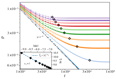
(a)

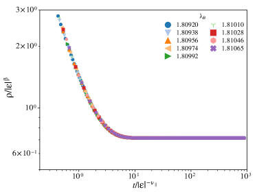
(b)

Figure 3: (a) The main plot shows $\left\langle\rho\left(t\right)\right\rangle$ vs $t$ in the active phase, for $k=1$ with $\mu=1$, $\lambda_{A}=1/2$ and distances to criticality from $\epsilon=9\times 10^{-4}$ to $\epsilon=0$, top to bottom. Symbols indicate estimates for the characteristic time $\xi_{t}$, whose log-log dependence on the distance to the critical point is shown in the inset. The estimates come from determining, for each curve, the time at which the average density reaches a value 10% above its asymptotic value. (b) Rescaled plots of the average density, showing data collapse following Eq. (32). Here, $\beta=\delta=\nu_{\parallel}=1$ are the values of the clean theory.

Plots of $\left\langle\rho\left(t\right)\right\rangle$ in the active phase and at the critical point are shown in Fig. 3a. It is clear that the behavior is quite similar to that of the uniform limit, as illustrated by the fact that all curves closely follow those obtained for a uniform system with the same average parameters as the corresponding aperiodic system. At the critical point, the behavior of $\left\langle\rho\left(t\right)\right\rangle$ is perfectly compatible with a power law $t^{-\delta}$, with $\delta=\beta/\nu_{\parallel}=1$ as in the uniform model. In fact, as shown in Fig. 3b, all curves can be collapsed onto the same scaling form

$$\rho\left(t;\epsilon\right)=\left|\epsilon\right|^{\beta}f\left(t\left|\epsilon\right|^{\nu_{\parallel}}\right),$$ (32)

with $\beta=\nu_{\parallel}=1$, in which $f\left(t\left|\epsilon\right|^{\nu_{\parallel}}\right)$ is a scaling function taking a constant value if $t\gg\left|\epsilon\right|^{-\nu_{\parallel}}\sim\xi_{t}$. For definiteness, we fixed both $\mu$ and $\lambda_{A}$ and use $\lambda_{B}$ as a tuning parameter to cross the transition at the critical value

$$\lambda_{B}^{*}=\frac{\mu\zeta_{+}-\lambda_{A}}{\zeta_{+}-1},$$ (33)

which is obtained from Eq. (16). In that case, the distance from criticality is defined as

$$\epsilon\equiv 1-\frac{\lambda_{B}}{\lambda_{B}^{*}}.$$ (34)

Figure 4: Plots of linear (left) and logarithmic (right) noise ratios at criticality for $k=1$ and different modulation strengths $\lambda_{A}/\lambda_{B}$. For a given modulation strength, the critical value of $\mu$ is determined by using Eq. (16).

The behavior of the ratios $\sigma_{\rho}\left(t\right)/\left\langle\rho\left(t\right)\right\rangle$ and $\sigma_{\ln\rho\left(t\right)}/\left\langle\ln\rho\left(t\right)\right\rangle$ at criticality is shown in Fig. 4. These plots can be understood by noticing that for $k=1$ and at large times, $\rho_{i}\left(t\right)\sim C_{i}t^{-1}$, in which $i$ labels a given sample and all $C_{i}$ are approximately the same, given the fact that fluctuations are small. Thus, denoting by $\sigma_{C}$ the standard deviation of the $C_{i}$, we have

$$\left\langle\rho\left(t\right)\right\rangle\sim\frac{\left\langle C_{i}\right\rangle}{t},\quad\sigma_{\rho}\left(t\right)\sim\frac{\sigma_{C}}{t},$$ (35)

so that

$$\frac{\sigma_{\rho}\left(t\right)}{\left\langle\rho\left(t\right)\right\rangle}\sim\frac{\left\langle C_{i}\right\rangle}{\sigma_{C}},$$ (36)

and the ratio $\sigma_{\rho}\left(t\right)/\left\langle\rho\left(t\right)\right\rangle$ should approach a constant at large times. Likewise, denoting by $\sigma_{\ln C}$ the standard deviation of $\ln C_{i}$,

$$\left\langle\ln\rho\left(t\right)\right\rangle=\left\langle\ln C_{i}\right\rangle-\ln t,\quad\sigma_{\ln\rho}=\sigma_{\ln C},$$

so that

$$\frac{\sigma_{\ln\rho}\left(t\right)}{\left\langle\ln\rho\left(t\right)\right\rangle}\sim\frac{\sigma_{\ln C}}{\left\langle\ln C_{i}\right\rangle-\ln t},$$

and the ratio $\sigma_{\ln\rho\left(t\right)}/\left\langle\ln\rho\left(t\right)\right\rangle$ should exhibit a weak time dependence at large times. These expectations are fully compatible with the numerical results shown in Fig. 4.

IV.2 Case $k=2$

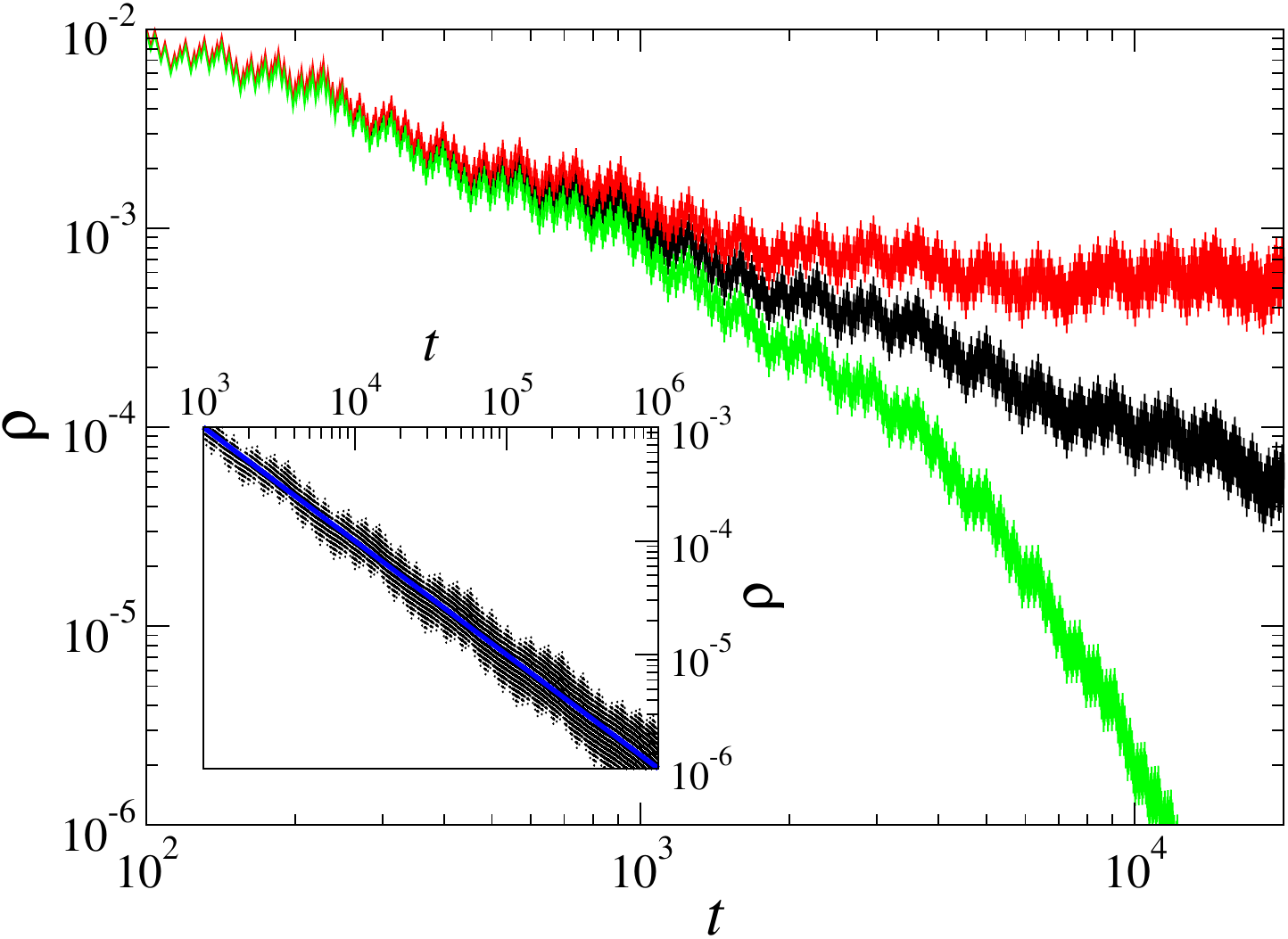
(a)

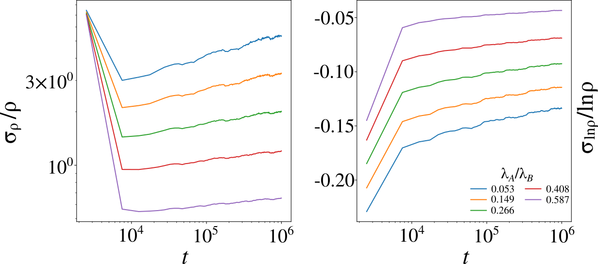
(b)

Figure 5: (a) The main plot shows $\rho\left(t\right)$ vs $t$ for a single sample with $k=2$, $\mu=1$, $\lambda_{A}=9/10$ and distances to criticality given by $\epsilon=-10^{-3}$ (upper red curve), $\epsilon=0$ (middle black curve), and $\epsilon=10^{-3}$ (lower green curve). The inset shows the long-time behavior of $\rho\left(t\right)$ at criticality, illustrating the slight increase in relative fluctuations over time (for clarity, points are not connected by lines). The thick blue curve is the function $\rho=1/t$. (b) Plots of linear (left) and logarithmic (right) noise ratios at criticality for $k=2$ and different modulation strengths $\lambda_{A}/\lambda_{B}$.

Now we analyze the marginal case $k=2$, which has a wandering exponent $\omega=0$. Figure 5a shows $\left\langle\rho\left(t\right)\right\rangle$ for different values of $\epsilon$. At the critical point the power-law $\left\langle\rho\left(t\right)\right\rangle\sim t^{-\delta}$ is still valid with $\delta=1$ as for $k=1$, but fluctuations are stronger. This is also noticeable from the behavior of the ratio $\sigma_{\rho}\left(t\right)/\left\langle\rho\left(t\right)\right\rangle$ at criticality, shown in Fig. 5b. At long times, the ratio no longer approaches a constant, but slightly increases as a power law with an exponent that depends on the ratio $\lambda_{A}/\lambda_{B}$. However, we cannot exclude the possibility of a logarithmic growth with a ratio-dependent coefficient. This nonuniversality is characteristic of marginal fluctuations. On the other hand, the ratio $\sigma_{\ln\rho\left(t\right)}/\left\langle\ln\rho\left(t\right)\right\rangle$ behaves similarly to the case $k=1$, approaching zero at long times. This suggests that, as time increases, the relative width of the distribution of $\rho_{i}\left(t\right)$ becomes larger, but that of $\ln\rho_{i}\left(t\right)$ becomes smaller.

IV.3 Case $k=3$

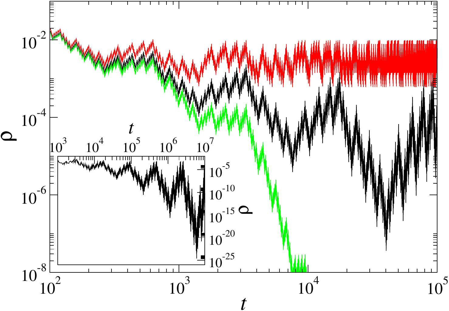
(a)

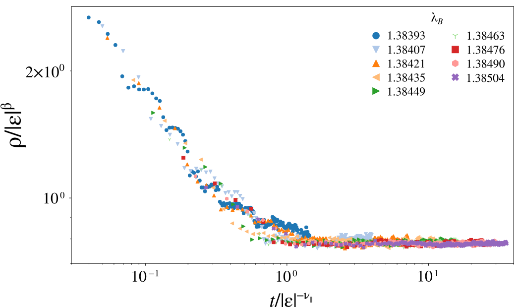
(b)

Figure 6: (a) The main plot shows $\rho\left(t\right)$ vs $t$ for a single sample with $k=3$, $\mu=1$, $\lambda_{A}=9/10$ and distances to criticality given by $\epsilon=-5\times 10^{-3}$ (upper red curve), $\epsilon=0$ (middle black curve), and $\epsilon=2\times 10^{-3}$ (lower green curve). The inset shows the long-time behavior of $\rho\left(t\right)$ exactly at criticality, illustrating the strong increase in relative fluctuations over time. (b) Rescaled plots of the average density for $k=3$, with $\mu=1$ and $\lambda_{A}=1/2$, showing data collapse following Eq. (32). Here, $\beta=1$ and $\nu_{\parallel}\approx 1.46$ [see Eq. (29)].

Finally, we study the case $k=3$ in which aperiodic temporal disorder is a relevant perturbation to the clean critical behavior. Here, the wandering exponent is $\omega\approx 0.317>\omega_{c}$ [see criterion (6)]. For a single sample, density fluctuations increase very strongly as a function of time at criticality, as shown in the inset of Fig. 6a. When averaged over many samples, the behavior is compatible with Eq. (32) with $\beta=1$ and $\nu_{\parallel}\approx 1.46$, in agreement with the RG prediction in Eq. (29), as shown in Fig. 6b.

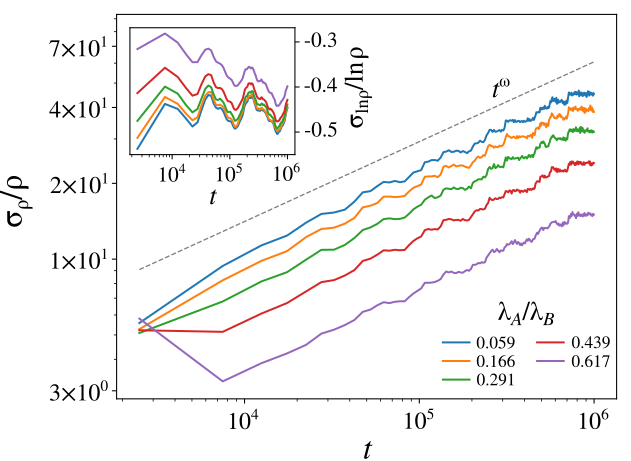
Figure 7: Linear (main plot) and logarithmic (inset) noise ratios at criticality for $k=3$ and different modulation strengths $\lambda_{A}/\lambda_{B}$.

As for the ratios $\sigma_{\rho}\left(t\right)/\left\langle\rho\left(t\right)\right\rangle$ and $\sigma_{\ln\rho\left(t\right)}/\left\langle\ln\rho\left(t\right)\right\rangle$ at criticality, we can see from Fig. 7 that $\sigma_{\rho}\left(t\right)/\left\langle\rho\left(t\right)\right\rangle$ follows a power-law with an exponent compatible with the wandering exponent $\omega$ corresponding to $k=3$. (Although not shown, we checked that the analogous behavior is also observed for other larger values of $k$.) Furthermore, the ratio $\sigma_{\ln\rho\left(t\right)}/\left\langle\ln\rho\left(t\right)\right\rangle$ tends to oscillate around a constant at long times. This indicates that, as time increases, the relative width of the distribution of $\rho_{i}\left(t\right)$ becomes larger, while that of $\ln\rho_{i}\left(t\right)$ remains constant. This should be compared with the behavior observed under random temporal disorder (Vojta and Hoyos, 2015; Wada et al., 2018), for which, at criticality, $\sigma_{\ln\rho\left(t\right)}\sim\left|\ln\rho_{i}\right|\sim t^{(2-\gamma)/2}\sim t^{H}$, also leading to a constant ratio $\sigma_{\ln\rho\left(t\right)}/\left\langle\ln\rho\left(t\right)\right\rangle$ at long times. Thus, our results indicate that, in the mean-field limit, any wandering exponent $\omega>0$ leads to “infinite-noise” critical behavior at long times.

V Conclusions

We have investigated the mean-field limit of the contact process in the presence of deterministic aperiodic temporal disorder induced by generalized Fibonacci sequences. These sequences have fluctuations which grows with time as $\sim t^{\omega}$, with a wandering exponent $\omega$ that depends of the parameter $k$ of the generalized sequences. More importantly, the value of $\omega$ can be tuned such that aperiodic temporal disorder can be a irrelevan, a marginal, or a relevant perturbation to the clean critical behavior. For $\omega<\omega_{c}$ ($k<2$), the long-time scaling behavior of the clean model remains unaltered, with relative density fluctuations decreasing over time. For $\omega=\omega_{c}$ ($k=2$), the aperiodic disorder induces density fluctuations which grow slightly over time, but the critical exponents remain unaltered. Finally, for $\omega>\omega_{c}$ ($k>2$), as in the case of random temporal disorder, the long-time behavior is dominated by diverging density fluctuations, and the critical behavior of the system is in the so-called “infinite-noise” universality class.

Nevertheless, contrary to the random case, aperiodic temporal disorder does not give rise to active (temporal) Griffiths phases. In the random case, these phases exist due to long (and rare) incursions of the system in the inactive phase, even though the system is in the active phase. These incursions allow the density to fall below any threshold value associated with the inverse population size. Thus, the system may reach the absorbing state even in the limit of an arbitrarily large population. The underlying inflation symmetry of the generalized Fibonacci sequences does not allow the formation of those long rare regions. However, sufficiently close to criticality, finite regions give rise to large fluctuations of the density at long times. This is illustrated in the upper red curve of the main plot in Fig. 6a.

The long-time behavior described above is in full agreement with the generalized criterion stated in Eq. (6). Such criterion can be further tested for the contact process in finite dimensions, as well as for other nonequilibrium models (Solano et al., 2016; Barghathi et al., 2017; Wada and Hoyos, 2021). It would also be interesting to investigate the effect of aperiodic temporal disorder on systems exhibiting first-order nonequilibrium phase transitions (de Oliveira and Fiore, 2016; Fiore et al., 2018; Encinas and Fiore, 2021).

Appendix A Properties of the generalized Fibonacci sequence

For the generalized Fibonacci sequence defined by the substitution rule $A\rightarrow AB^{k}$ and $B\rightarrow A$, the numbers $N_{A}^{\left(j\right)}$ and $N_{B}^{\left(j\right)}$ of letters $A$ and $B$ in the finite sequence obtained after $j$ iterations of the rule are given by the matrix equation

$$\left(\begin{array}[]{c}N_{A}^{\left(j\right)}\\ N_{B}^{\left(j\right)}\end{array}\right)=\boldsymbol{\Omega}^{j}\left(\begin{array}[]{c}1\\ 0\end{array}\right),$$ (37)

in which we assume that the sequence is built starting from a single letter $A$ and $\boldsymbol{\Omega}$ is the substitution matrix

$$\boldsymbol{\Omega}=\left(\begin{array}[]{cc}1&1\\ k&0\end{array}\right).$$ (38)

Diagonalizing $\boldsymbol{\Omega}$, we can write

$$\boldsymbol{\Omega}=\mathbf{U}\left(\begin{array}[]{cc}\zeta_{+}&0\\ 0&\zeta_{-}\end{array}\right)\mathbf{U}^{-1},\qquad\mathbf{U}=\left(\begin{array}[]{cc}\zeta_{-}/k&\zeta_{+}/k\\ 1&1\end{array}\right),$$ (39)

with

$$\zeta_{\pm}=\frac{1\pm\sqrt{1+4k}}{2},$$ (40)

so that

$$\boldsymbol{\Omega}^{j}=\mathbf{U}\left(\begin{array}[]{cc}\zeta_{+}^{j}&0\\ 0&\zeta_{-}^{j}\end{array}\right)\mathbf{U}^{-1},$$ (41)

leading to

$$N_{A}^{\left(j\right)}=\frac{\zeta_{+}^{j+1}-\zeta_{-}^{j+1}}{\sqrt{4k+1}},\quad N_{B}^{\left(j\right)}=k\frac{\zeta_{+}^{j}-\zeta_{-}^{j}}{\sqrt{4k+1}}.$$ (42)

Taking into account that $\zeta_{+}>\left|\zeta_{-}\right|$, the asymptotic fractions of letters $A$ and $B$ are, respectively,

$$x_{A}=\lim_{j\rightarrow\infty}\frac{N_{A}^{\left(j\right)}}{N_{j}}=\frac{1}{\zeta_{+}}$$ (43)

and

$$x_{B}=\lim_{j\rightarrow\infty}\frac{N_{B}^{\left(j\right)}}{N_{j}}=1-\frac{1}{\zeta_{+}},$$ (44)

and thus,

$$N_{j}=N_{A}^{\left(j\right)}+N_{B}^{\left(j\right)}\sim\zeta_{+}^{j+2}.$$ (45)

On the other hand, the fluctuations in the number of letters with respect to the asymptotic expectation values, gauged by

$$G_{j}=\left|N_{A}^{\left(j\right)}-x_{A}N_{j}\right|,$$ (46)

are governed by

$$G_{j}\approx\frac{1}{\sqrt{4k+1}}\left|\zeta_{-}^{j}\left[\zeta_{-}-x_{A}\left(\zeta_{-}-k\right)\right]\right|\propto\left|\zeta_{-}^{j}\right|\propto N_{j}^{\omega},$$ (47)

which defines the wandering exponent

$$\omega=\frac{\ln\left|\zeta_{-}\right|}{\ln\zeta_{+}}.$$ (48)

If $\omega<0$, the geometrical fluctuations get smaller as the sequence gets larger, and at long times the behavior should recover that of the uniform limit. On the other hand, if $\omega>0$, fluctuations become larger and larger. The case $\omega=0$ is marginal and may give rise to nonuniversal behavior. For the generalized Fibonacci sequence, we have $\omega=-1<0$ for $k=1$, $\omega=0$ for $k=2$, and $\omega\approx 0.317>0$ for $k\geq 3$.

Appendix B Diagonalizing the matrix $\mathbf{M}$

The matrix $\mathbf{M}$ in Eq. (19) can be written as

$$\mathbf{M}=\mathbf{V}\left(\begin{array}[]{ccc}1&0&0\\ 0&\Xi_{-}&0\\ 0&0&\Xi_{+}\end{array}\right)\mathbf{V}^{-1},$$ (49)

with $\Xi_{\pm}$ given by Eq. (23) and

$$\mathbf{V}=\left(\begin{array}[]{ccc}-1&-\zeta_{+}/k&-\zeta_{-}/k\\ 1&\Xi_{+}/k^{2}&\Xi_{-}/k^{2}\\ 1&1&1\end{array}\right).$$ (50)

Therefore,

$$\mathbf{M}^{j}=\mathbf{V}\left(\begin{array}[]{ccc}1&0&0\\ 0&\Xi_{-}^{j}&0\\ 0&0&\Xi_{+}^{j}\end{array}\right)\mathbf{V}^{-1}.$$ (51)

Using

$$\left(\begin{array}[]{c}\ln r_{0}^{++}\\ \ln r_{0}^{-}\\ \ln r_{0}^{--}\end{array}\right)=\left(\begin{array}[]{c}k\left(\mu-\lambda_{B}\right)\\ \mu-\lambda_{A}\\ \left(k+1\right)\left(\mu-\lambda_{A}\right)\end{array}\right)$$ (52)

and

$$\left(\begin{array}[]{c}\Delta t_{0}^{++}\\ \Delta t_{0}^{-}\\ \Delta t_{0}^{--}\end{array}\right)=\left(\begin{array}[]{c}k\\ 1\\ k+1\end{array}\right)\Delta t$$ (53)

in Eqs. (17) and (18), we obtain Eqs. (21) and (22) with

$$\eta_{0}=\frac{\left(\mu-\lambda_{A}\right)-k\left(\mu-\lambda_{B}\right)}{k-2}=-\eta_{1}=-\eta_{2},$$ (54)

$$\eta_{0}^{\pm}=\mp\Delta\left[\left(\Xi_{\pm}-k^{2}\right)\left(\mu-\lambda_{A}\right)+k\left(\zeta_{\pm}+k\zeta_{\mp}\right)\left(\mu-\lambda_{B}\right)\right],$$ (55)

$$\eta_{1}^{\pm}=\mp\Delta\left[\left(\zeta_{\pm}+k\zeta_{\mp}\right)\left(\mu-\lambda_{A}\right)+k\left(\zeta_{\pm}-k\right)\left(\mu-\lambda_{B}\right)\right],$$ (56)

$$\eta_{2}^{\pm} = \mp\Delta\left\{\left[\Xi_{\pm}-k\left(k-1\right)\zeta_{\pm}\right]\left(\mu-\lambda_{A}\right)\right.$$ (57)

$$+\left.k\left(\Xi_{\pm}-k^{2}\right)\left(\mu-\lambda_{B}\right)\right\},$$

$$\tau_{0}=-\frac{k-1}{k-2}=-\tau_{1}=-\tau_{2},$$ (58)

$$\tau_{0}^{\pm}=\mp\Delta\left[\left(\Xi_{\pm}-k^{2}\right)+k\left(\zeta_{\pm}+k\zeta_{\mp}\right)\right],$$ (59)

$$\tau_{1}^{\pm}=\mp\Delta\left(\zeta_{\pm}-k\left(k-1\right)\right),$$ (60)

$$\tau_{2}^{\pm}=\mp\Delta\left[\left(k+1\right)\Xi_{\pm}-k\left(k-1\right)\zeta_{\pm}-k^{3}\right],$$ (61)

in which

$$\Delta^{-1}=\left(k-2\right)\sqrt{1+4k}.$$ (62)

It is interesting to notice that

$$\eta_{i}^{\pm}=\gamma_{i}^{\pm}\left(\mu-\frac{1}{\zeta_{\pm}}\lambda_{A}-\left(1-\frac{1}{\zeta_{\pm}}\right)\lambda_{B}\right),$$ (63)

where $\gamma_{0}^{\pm}=\pm\Delta\left(\zeta_{\pm}\left(k^{2}-k-1\right)-k\right)$, $\gamma_{1}^{\pm}=\pm\Delta\left(k\left(k-1\right)-\zeta_{\pm}\right)$, and $\gamma_{2}^{\pm}=\pm\Delta\left(k\left(k^{2}-1\right)-\left(2k+1\right)\zeta_{\pm}-k^{2}\zeta_{\mp}\right)$. It is easy to show that $\eta_{i}^{+}>0$ for $k\geq 0$.

For $k=2$, $\eta_{i}$, $\eta_{i}^{-}$, $\tau_{i}$ and $\tau_{i}^{-}$ are divergent. However, the following useful quantities remain finite:

$$\lim_{k\rightarrow 2}\left(\eta_{0}+\eta_{0}^{-}\right)=\frac{2}{9}\left(\mu+4\lambda_{A}-5\lambda_{B}\right),$$ (64)

$$\lim_{k\rightarrow 2}\left(\eta_{1}+\eta_{1}^{-}\right)=\frac{1}{9}\left(\mu-5\lambda_{A}-4\lambda_{B}\right),$$ (65)

$$\lim_{k\rightarrow 2}\left(\eta_{2}+\eta_{2}^{-}\right)=\frac{1}{9}\left(-5\mu-11\lambda_{A}+16\lambda_{B}\right),$$ (66)

$$\lim_{k\rightarrow 2}\eta_{0}^{+}=\frac{16}{9}\left[\mu-\frac{1}{2}\left(\lambda_{A}+\lambda_{B}\right)\right],$$ (67)

$$\lim_{k\rightarrow 2}\eta_{1}^{+}=\frac{8}{9}\left[\mu-\frac{1}{2}\left(\lambda_{A}+\lambda_{B}\right)\right],$$ (68)

$$\lim_{k\rightarrow 2}\eta_{2}^{+}=\frac{32}{9}\left[\mu-\frac{1}{2}\left(\lambda_{A}+\lambda_{B}\right)\right],$$ (69)

$\lim_{k\rightarrow 2}\left(\tau_{0}+\tau_{0}^{-}\right)=\frac{2}{9},$ $\lim_{k\rightarrow 2}\left(\tau_{1}+\tau_{1}^{-}\right)=\frac{1}{9},$ $\lim_{k\rightarrow 2}\left(\tau_{2}+\tau_{2}^{-}\right)=-\frac{5}{9},$$\lim_{k\rightarrow 2}\tau_{0}^{+}=\frac{16}{9},$ $\lim_{k\rightarrow 2}\tau_{1}^{+}=\frac{8}{9},$ and $\lim_{k\rightarrow 2}\tau_{2}^{+}=\frac{32}{9}$.

References

- Marro and Dickman (2006) J. Marro and R. Dickman, Nonequilibrium Phase Transitions in Lattice Models (Cambrige University Press, 2006).
- Hinrichsen (2000) H. Hinrichsen, Advances in Physics 49, 815 (2000).
- Takeuchi et al. (2007) K. A. Takeuchi, M. Kuroda, H. Chaté, and M. Sano, Phys. Rev. Lett. 99, 234503 (2007).
- Alcaraz et al. (1994) F. Alcaraz, M. Droz, M. Henkel, and V. Rittenberg, Annals of Physics 230, 250 (1994).
- Murray (2007) J. D. Murray, Mathematical Biology I: An Introduction (Springer, 2007).
- Harris (1974a) T. E. Harris, Ann. Prob. 2, 969 (1974a).
- Tomé and Oliveira (2015) T. Tomé and M. J. Oliveira, Stochastic Dynamics and Irreversibility (Springer, 2015).
- Faria et al. (2008) M. S. Faria, D. J. Ribeiro, and S. R. Salinas, Journal of Statistical Mechanics: Theory and Experiment 2008, P01022 (2008).
- Barghathi et al. (2014) H. Barghathi, D. Nozadze, and T. Vojta, Phys. Rev. E 89, 012112 (2014).
- Ódor (2004) G. Ódor, Rev. Mod. Phys. 76, 663 (2004).
- Noest (1986) A. J. Noest, Phys. Rev. Lett. 57, 90 (1986).
- Hooyberghs et al. (2003) J. Hooyberghs, F. Iglói, and C. Vanderzande, Phys. Rev. Lett. 90, 100601 (2003).
- Vojta and Dickison (2005) T. Vojta and M. Dickison, Phys. Rev. E 72, 036126 (2005).
- Vojta and Lee (2006) T. Vojta and M. Y. Lee, Phys. Rev. Lett. 96, 035701 (2006).
- Hoyos (2008) J. A. Hoyos, Phys. Rev. E 78, 032101 (2008).
- Vazquez et al. (2011) F. Vazquez, J. A. Bonachela, C. López, and M. A. Muñoz, Phys. Rev. Lett. 106, 235702 (2011).
- Vojta and Hoyos (2015) T. Vojta and J. A. Hoyos, EPL (Europhysics Letters) 112, 30002 (2015).
- Barghathi et al. (2016) H. Barghathi, T. Vojta, and J. A. Hoyos, Phys. Rev. E 94, 022111 (2016).
- de Oliveira and Fiore (2016) M. M. de Oliveira and C. E. Fiore, Phys. Rev. E 94, 052138 (2016).
- Solano et al. (2016) C. M. D. Solano, M. M. de Oliveira, and C. E. Fiore, Phys. Rev. E 94, 042123 (2016).
- Wada et al. (2018) A. H. O. Wada, M. Small, and T. Vojta, Phys. Rev. E 98, 022112 (2018).
- Fiore et al. (2018) C. E. Fiore, M. M. de Oliveira, and J. A. Hoyos, Phys. Rev. E 98, 032129 (2018).
- Encinas and Fiore (2021) J. M. Encinas and C. E. Fiore, Phys. Rev. E 103, 032124 (2021).
- Wada and Hoyos (2021) A. H. O. Wada and J. A. Hoyos, Phys. Rev. E 103, 012306 (2021).
- Luck (1993) J. M. Luck, Europhysics Letters (EPL) 24, 359 (1993).
- Harris (1974b) A. B. Harris, Journal of Physics C: Solid State Physics 7, 1671 (1974b).
- Kinzel (1985) W. Kinzel, Z. Physik B – Condensed Matter 58, 229 (1985).
- Vojta and Dickman (2016) T. Vojta and R. Dickman, Phys. Rev. E 93, 032143 (2016).
- Barghathi et al. (2017) H. Barghathi, S. Tackkett, and T. Vojta, The European Physical Journal B 90, 129 (2017).