Forward-PECVaR Algorithm: Exact Evaluation for CVaR SSPs

Abstract.

The Stochastic Shortest Path (SSP) problem models probabilistic sequential-decision problems where an agent must pursue a goal while minimizing a cost function. Because of the probabilistic dynamics, it is desired to have a cost function that considers risk. Conditional Value at Risk (CVaR) is a criterion that allows modeling an arbitrary level of risk by considering the expectation of a fraction $\displaystyle\alpha$ of worse trajectories. Although an optimal policy is non-Markovian, solutions of CVaR-SSP can be found approximately with Value Iteration based algorithms such as CVaR Value Iteration with Linear Interpolation (CVaRVILI) and CVaR Value Iteration via Quantile Representation (CVaRVIQ). These type of solutions depends on the algorithm’s parameters such as the number of atoms and $\displaystyle\alpha_{0}$ (the minimum $\displaystyle\alpha$). To compare the policies returned by these algorithms, we need a way to exactly evaluate stationary policies of CVaR-SSPs. Although there is an algorithm that evaluates these policies, this only works on problems with uniform costs. In this paper, we propose a new algorithm, Forward-PECVaR (ForPECVaR), that evaluates exactly stationary policies of CVaR-SSPs with non-uniform costs. We evaluate empirically CVaR Value Iteration algorithms that found solutions approximately regarding their quality compared with the exact solution, and the influence of the algorithm parameters in the quality and scalability of the solutions. Experiments in two domains show that it is important to use an $\displaystyle\alpha_{0}$ smaller than the $\displaystyle\alpha$ target and an adequate number of atoms to obtain a good approximation.

1. Introduction

The Stochastic Shortest Path (SSP) problem models probabilistic sequential-decision problems where an agent must pursue a goal while minimizing a cost function. Because of the probabilistic dynamics, it is desired to have a cost function that considers risk. Several measures for measuring financial risk have been constantly studied and applied in different sectors. These measures include variance, Value at Risk (VaR), and Conditional Value at Risk (CVaR). Conditional Value at Risk (CVaR) is a coherent risk measure Rockafellar and Uryasev (2002) criterion that allows modeling an arbitrary level of risk by considering the expectation of a fraction $\displaystyle\alpha$ of worse trajectories in sequential-decision problems Bäuerle and Ott (2011); Chow et al. (2015); Stanko and Macek (2019).

Although an optimal policy for CVaR-SSPs is non-Markovian (depends on the entire history of actions and states visited so far), solutions of CVaR-SSP can be found approximately with Value Iteration based algorithms. One algorithm that finds a policy for CVaR-SSPs is the CVaR Value Iteration with Linear Interpolation, referred to as CVaRVILI Chow et al. (2015). The policy returned by the CVaRVILI algorithm is stationary (it does not depend on time) and non-Markovian policy. This algorithm is very costly as it needs to solve several linear programming problems. Another algorithm that finds a stationary and non-Markovian policy is CVaR Value Iteration via Quantile Representation, referred to as CVaRVIQ Stanko and Macek (2019). CVaRVIQ uses distributional approach techniques to find the solutions faster than CVaRVILI. The solutions that can be found approximately depend on the algorithm’s parameters such as the number of atoms and $\displaystyle\alpha_{0}$ (the minimum $\displaystyle\alpha$). Due to the approximate approach, the exact value of the policy is not found, although it is possible to approximate it as much as desired by using a greater number of atoms, which implies an increase in the computational cost.

To compare the policies returned by these algorithms, we need a way to exactly evaluate the stationary policies of CVaR-SSPs. Although there is an algorithm that evaluates these policies, this only works on problems with uniform cost Meggendorfer (2022). In this paper, we propose a new algorithm, ForPECVaR (Forward Policy Evaluation CVaR), that evaluates exactly stationary policies of CVaR-SSPs with non-uniform cost. To work with this type of cost, ForPECVaR tracks the accumulated cost for each trajectory from the initial state independently.

Thus, ForPECVaR could be used to compare approximate solutions. To the best of our knowledge, there is no algorithm that exactly evaluates the policies returned by CVaRVILI, CVaRVIQ, and other similar algorithms for problems with non-uniform costs. ForPECVaR can also be used as the policy evaluation step of a possible Policy Iteration algorithm. Additionally, ForPECVaR also calculates the exact VaR value of the policies that can be used by other algorithms such as the algorithm proposed in Rigter et al. (2022).

In this paper, we perform experiments to compare the approximate values returned by CVaRVILI and CVaRVIQ with the exact values computed by ForPECVaR, and the influence of the algorithm parameters ($\displaystyle\alpha_{0}$ and number of atoms) in the quality and scalability of the solutions in two domains.

2. Background

2.1. Stochastic Shortest Path Problem

A Stochastic Shortest Path Problem Bertsekas and Tsitsiklis (1991) is described by a tuple $\displaystyle\mathcal{M}=\langle\mathcal{S},\mathcal{A},P,c,\mathcal{G}\rangle$ where: $\displaystyle\mathcal{S}$ is a finite set of states; $\displaystyle\mathcal{A}$ is a finite set of actions; $\displaystyle P:\mathcal{S}\times\mathcal{A}\times\mathcal{S}\rightarrow[0,1]$ is a transition function that represents the probability that $\displaystyle s^{\prime}\in\mathcal{S}$ is reached after the agent executes an action $\displaystyle a\in\mathcal{A}$ in a state $\displaystyle s\in\mathcal{S}$, i.e., $\displaystyle\Pr(s_{t+1}=s^{\prime}|s_{t}=s,a_{t}=a)=P(s,a,s^{\prime})$; $\displaystyle c:\mathcal{S}\times\mathcal{A}\rightarrow\mathcal{R}^{+}$ is a positive cost function that represents the cost of executing an action $\displaystyle a\in\mathcal{A}$ in a state $\displaystyle s\in\mathcal{S}$, i.e., $\displaystyle c_{t}=c(s_{t},a_{t})$; and $\displaystyle\mathcal{G}$ is a non-empty set of goal states that are absorbing, i.e., $\displaystyle P(s_{t+1}\in\mathcal{G}|s_{t}\in\mathcal{G},a_{t}=a)=1$ and $\displaystyle c(s_{t}\in\mathcal{G},a_{t}=a)=0$ for all $\displaystyle a\in\mathcal{A}$.

The solution to an SSP is a policy $\displaystyle\pi$ that could be:

• Stationary ($\displaystyle\pi:\mathcal{S}\to\mathcal{A}$) that maps every state $\displaystyle s_{t}$ into an action $\displaystyle a_{t}=\pi(s_{t})$;

• Non-Markovian or history-dependent ($\displaystyle\Pi_{H}$). Let $\displaystyle H_{t}=H_{t-1}\times\mathcal{A}\times\mathcal{S}$ be the space of histories up to time $\displaystyle t\geq 1$ and $\displaystyle H_{0}=\mathcal{S}$ where each history $\displaystyle h_{t}\in H_{t}$ is $\displaystyle h_{t}=(s_{0},a_{0},\cdots,s_{t-1},a_{t-1},s_{t})$. Let $\displaystyle\Pi_{H,t}$ be the set of all history-dependent policies up to time $\displaystyle t$ with the property that at each time $\displaystyle t$ the action is a function of $\displaystyle h_{t}$, i.e., $\displaystyle\Pi_{H,t}=(\mu_{0}:H_{0}\rightarrow\mathcal{A},\mu_{1}:H_{1}\rightarrow\mathcal{A},\cdots,\mu_{t}:H_{t}\rightarrow\mathcal{A})$, then $\displaystyle\Pi_{H}=\lim_{t\rightarrow\infty}\Pi_{H,t}$ the set of all history-dependent policies.

Let the random variable $\displaystyle Z_{M}=\sum_{t=0}^{M}c\mathopen{}\left({s_{t},\pi(s_{t})}\,\negthickspace\right)\mathclose{}$ be the accumulated cost from time $\displaystyle 0$ up to time $\displaystyle M$. The value function of a policy $\displaystyle\pi$ is defined by the total expected cost of reaching the goal from $\displaystyle s_{0}$:

$$V^{\pi}(s)=\lim_{M\to\infty}\text{E}\left[\left.Z_{M}\right|\pi,s_{0}=s\right].$$ (1)

A policy $\displaystyle\pi$ is proper if $\displaystyle\lim_{t\rightarrow\infty}\Pr(s_{t}\in\mathcal{G}|\pi,s_{0}=s)=1$, $\displaystyle\forall{s\in\mathcal{S}}$ Bertsekas and Tsitsiklis (1991). The value function $\displaystyle V^{\pi}(s)$ for SSPs is well-defined only for proper policies. Any improper policy has an infinite value $\displaystyle V^{\pi}(s)=\infty$ at every state $\displaystyle s$ that cannot reach a goal state with probability 1.

The value of a proper policy $\displaystyle\pi$ can be found using the equation:

$$V^{\pi}(s)=\begin{cases}0&\text{, if }s\in\mathcal{G}\\ c(s,\pi(s))+\displaystyle\sum_{s^{\prime}\in\mathcal{S}}T(s,\pi(s),s^{\prime})V^{\pi}(s^{\prime})&\text{, otherwise.}\end{cases}$$ (2)

The optimal value $\displaystyle V^{*}(s)=\displaystyle\min_{\pi}V^{\pi}(s)$ can be computed by solving the Bellman equation:

$$V^{*}(s)=\begin{cases}0&\text{, if }s\in\mathcal{G}\\ \displaystyle\min_{a\in\mathcal{A}}\left[c(s,a)+\displaystyle\sum_{s^{\prime}\in\mathcal{S}}T(s,a,s^{\prime})V^{*}(s^{\prime})\right]&\text{, otherwise.}\end{cases}$$ (3)

An optimal policy can be extracted from $\displaystyle V^{*}$ by:

$$\pi^{*}(s)\in\displaystyle\arg\min_{a\in\mathcal{A}}\left[c(s,a)+\displaystyle\sum_{s^{\prime}\in\mathcal{S}}T(s,a,s^{\prime})V^{*}(s^{\prime})\right].$$ (4)

2.2. VaR and CVaR metrics

The VaR (Value at Risk) and CVaR (Conditional-Value-at-Risk) metrics are widely used for portfolio management of financial assets. VaR measures the worst expected loss within a given $\displaystyle\alpha$ confidence level, where $\displaystyle\alpha\in(0,1)$. VaR is defined as the $\displaystyle 1-\alpha$ quantile of Z, i.e.: $\displaystyle VaR_{\alpha}(Z)=\min\{z|F(z)\geq 1-\alpha\}$, where Z is a random variable (the accumulated cost in SSPs) and $\displaystyle F(z)$ is the cumulative distribution function.

An alternative measure is the CVaR metric which is computed by averaging losses that exceed the VaR value. CVaR, with a confidence level $\displaystyle\alpha\in(0,1)$ is defined as:

$$CVaR_{\alpha}(Z)=\min_{w\in\mathbb{R}}\mathopen{}\left\{{w+\frac{1}{\alpha}\mathbb{E}\mathopen{}\left[{(Z-w)^{+}}\,\negthickspace\right]\mathclose{}}\,\negthickspace\right\}\mathclose{},$$ (5)

where $\displaystyle(x)^{+}$ = max$\displaystyle\{x,0\}$ represents the positive part of $\displaystyle x$, and $\displaystyle w$ represents the decision variable that, at the optimum point, reaches the value of VaR, i.e., $\displaystyle CVaR_{\alpha}(Z)=VaR_{\alpha}(Z)+\frac{1}{\alpha}\mathbb{E}\mathopen{}\left[{(Z-VaR_{\alpha}(Z))^{+}}\,\negthickspace\right]\mathclose{}.$

There is a dual representation of CVaR that is used in sequential decision-making problems, defined as:

$$CVaR_{\alpha}(Z)=\max_{\xi\in\mathcal{U}_{CVaR}(\alpha,\mathbb{P})}\mathbb{E}_{\xi}[Z],$$ (6)

where $\displaystyle\mathbb{E}_{\xi}[Z]$ is the $\displaystyle\xi$-weighted expectation of Z, $\displaystyle\mathcal{U}_{CVaR}$ is the risk envelope Chow et al. (2015) that is represented by:

$$\displaystyle\mathcal{U}_{CVaR}(\alpha,\mathbb{P})=\Bigg{\{}\xi:\xi(\omega)\in \displaystyle\mathopen{}\left[{0,\frac{1}{\alpha}}\,\negthickspace\right]\mathclose{},\int_{\omega\in\Omega}\xi(\omega)\mathbb{P}(\omega)d\omega=1\Bigg{\}},$$ (7)

where $\displaystyle\mathbb{P}$ is a probability measure and $\displaystyle\Omega$ is the sample space. The risk envelope can be viewed as a set of probability measures that provides alternatives to $\displaystyle\mathbb{P}$ Chow et al. (2015).

2.3. CVaR Stochastic Shortest Path Problem

A CVaR SSP Chow et al. (2015) is defined by the tuple $\displaystyle\mathcal{M}_{CVaR}=\langle\mathcal{M},\alpha\rangle$ where $\displaystyle\mathcal{M}$ is an SSP and $\displaystyle\alpha\in(0,1]$ is the confidence level. Remember that $\displaystyle\Pi_{H}$ is the set of history-dependent policies. The objective in CVaR SSPs is to find $\displaystyle\mu\in{\Pi_{H}}$ Chow et al. (2015):

$$\min_{\mu\in\Pi_{H}}CVaR_{\alpha}\Bigg{(}\sum_{t=0}^{\infty}c(s_{t},a_{t})|s_{0}=s,\mu\Bigg{)},$$ (8)

where $\displaystyle\mu=\{\mu_{0},\mu_{1},...\}$ is the policy sequence that depends on the history with actions $\displaystyle a_{t}=\mu_{t}(h_{t})$ for $\displaystyle t\in\{0,1,...\}$.

A dynamic programming formulation for the CVaR SSP problem was proposed by Chow et al. Chow et al. (2015) by defining the CVaR value function $\displaystyle V$ over an augmented state space $\displaystyle\mathcal{S}\times Y$, where $\displaystyle Y=(0,1]$ is a continuous confidence level.

$$V(s,y)=\min_{\mu\in\Pi_{H}}CVaR_{y}\Bigg{(}\sum_{t=0}^{\infty}c(s_{t},a_{t})|s_{0}=s,\mu\Bigg{)}.$$ (9)

The Bellman operator $\displaystyle T:\mathcal{S}\times Y\rightarrow\mathcal{S}\times Y$ is defined by Chow et al. (2015):

$$\displaystyle T \displaystyle[V]\big{(}s,y\big{)}=\min_{a\in\mathcal{A}}\Bigg{[}c(s,a)+$$

$$\displaystyle\gamma\max_{\xi\in\mathcal{U}_{CVAR}(y,P(.|s,a))}\sum_{s^{\prime}\in\mathcal{S}}\xi(s^{\prime})V\Big{(}s^{\prime},y\xi(s^{\prime})\Big{)}P(s^{\prime}|s,a)\Bigg{]},$$ (10)

where the risk envelope $\displaystyle\mathcal{U}_{CVAR}$ is defined in Eq. 7. This operator has two properties: contraction and concavity preserving in $\displaystyle y$ Chow et al. (2015). The solution of $\displaystyle T[V](s,y)=V(s,y)$ is unique and equals to $\displaystyle V^{*}(s,y)=\min_{\mu\in\Pi_{H}}CVaR_{y}\Bigg{(}\sum_{t=0}^{\infty}c(s_{t},a_{t})|s_{0}=s,\mu\Bigg{)}$. The optimal policy can be obtained by a stationary Markovian policy, over the augmented state, defined as a greedy policy with respect to the value function $\displaystyle V^{*}(s,y)$.

The connection between an optimal history-dependent policy and a Markovian optimal policy on the augmented state space is given by the following theorem:

Theorem 1.

(Optimal Policies Chow et al. (2015)) Let $\displaystyle\pi^{*}_{H}=\{\mu_{0},\mu_{1},\cdots\}\in\Pi_{H}$ a history-dependent policy recursively defined as:

$$\mu_{k}(h_{k})=u^{*}(s_{k},y_{k}),\forall{k\geq 0},$$ (11)

with initial conditions $\displaystyle s_{0}$ and $\displaystyle y_{0}=\alpha$, and augmented state transitions

$$s_{k}\sim P(\cdot|s_{k-1},u^{*}(s_{k-1},y_{k-1})),\quad y_{k}=y_{k-1}\xi^{*}_{s_{k-1},y_{k-1},u^{*}}(s_{k}),\forall{k\geq 1},$$

where the stationary Markovian policy $\displaystyle u^{*}(s,y)$ and risk factor $\displaystyle\xi^{*}_{s,y,u^{*}}(\cdot)$ are solutions to the min-max optimization problem in the CVaR Bellman operator $\displaystyle T[V^{*}](s,y)$. Then, $\displaystyle\pi^{*}_{H}$ is an optimal policy for the CVaR SSP problem (8) with initial state $\displaystyle s_{0}$ and CVaR confidence level $\displaystyle\alpha$.

Among the algorithms that solve CVaR SSPs are CVaRVILI and CVaRVIQ.

2.3.1. CVaRVILI algorithm Chow et al. (2015)

This algorithm makes a discretization of $\displaystyle Y$ creating a set of interpolation points (also called a set of interpolation atoms) and interpolates the value function among these points. Let $\displaystyle N$ be the number of interpolation points (atoms) and for all $\displaystyle s\in\mathcal{S}$, let $\displaystyle Y(s)=(y_{1},y_{2},...,y_{N(s)})\in[0,1]^{N(s)}$ be the set of interpolation points. The linear interpolation of $\displaystyle yV(s,y)$ on these points is defined by:

$$I_{s}[V](y)=\begin{cases}y_{i}V(s,y_{i})\hskip 113.81102pt\text{, if }y\in Y\\ y_{i}V(s,y_{i})+\frac{y_{i+1}V(s,y_{i+1})-y_{i}V(s,y_{i})}{y_{i+1}-y_{i}}(y-y_{i}),\\ \hskip 153.6447pt\text{otherwise,}\end{cases}$$

where $\displaystyle y_{i}=\max\{y^{\prime}\in Y(s):y^{\prime}\leq y\}$ and $\displaystyle y_{i+1}=\min\{y^{\prime}\in Y(s):y^{\prime}\geq y\}$ such that $\displaystyle y\in$ $\displaystyle[y_{i},y_{i+1}]$; i.e, we use the two nearest points of $\displaystyle y$, called $\displaystyle y_{i}$ and $\displaystyle y_{i+1}$. Since $\displaystyle I_{s^{\prime}}[V]\big{(}y\xi(s^{\prime})\big{)}$ is the linear interpolation of $\displaystyle y\xi(s^{\prime})V\big{(}s^{\prime},y\xi(s^{\prime})\big{)}$, in Eq. 10 we can replace $\displaystyle\xi(s^{\prime})V\big{(}s^{\prime},y\xi(s^{\prime})\big{)}$ by $\displaystyle\frac{I_{s^{\prime}}[V](y\xi(s^{\prime}))}{y}$, obtaining the following interpolated Bellman operator $\displaystyle T_{I}$ Chow et al. (2015):

$$\displaystyle Q\big{(}s,y,a\big{)}=c(s,a)+\gamma\max_{\xi\in\mathcal{U}_{CVAR}(y,P(.|s,a))}\sum_{s^{\prime}\in S}\frac{I_{s^{\prime}}[V]\big{(}y\xi(s^{\prime})\big{)}}{y}P(s^{\prime}|s,a)$$

$$\displaystyle\centering T_{I}[V]\big{(}s,y\big{)}=\@add@centering \displaystyle\min_{a\in{A}}\{Q(s,y,a)\}.$$

CVaRVILI algorithm can have a high computational cost due to the need to solve many linear programming problems ($\displaystyle|S|\times|Y|\times|A|$ solver calls for each iteration). The greater the number of interpolation points $\displaystyle|Y|$, the smaller the approximation error, but the larger the computational time Chow et al. (2015).

2.3.2. CVaRVIQ algorithm Stanko and Macek (2019)

This algorithm is inspired by the use of the distributional approach of Bellemare et al Bellemare et al. (2017). The connection between the function $\displaystyle yCVaR_{y}$ and the quantile function ($\displaystyle VaR_{y}$) of the distribution of $\displaystyle Z$ are given by the convexity and piecewise linear properties of $\displaystyle yCVaR_{y}$ function, which means that $\displaystyle yCVaR_{y}$ can be obtained by:

$$yCVaR_{y}(Z)=\int_{0}^{y}VaR_{\beta}(Z)d\beta.$$ (12)

Additionally, $\displaystyle VaR_{y}$ can be obtained by:

$$\frac{\partial}{\partial Z}yCVaR_{y}(Z)=VaR_{y}(Z).$$ (13)

CVaRVIQ algorithm uses these properties to make faster computations. For each augmented state $\displaystyle(s,y)$ and for each action $\displaystyle a$, the distribution of the values of each successor augmented state is extracted with the application of Eq. 13 and then combined in another distribution considering the transition probability of each successor. Finally, the new distribution is transformed in the value function $\displaystyle Q(s,y,a)$ with Eq. 12.

The implementation of the CVaRVIQ algorithm returns the policy, CVaR, and VaR of all augmented states and does not return $\displaystyle\xi$. The $\displaystyle\xi$ function (necessary to guide the process of the variable $\displaystyle y$) can be computed by Stanko and Macek (2019):

$$\xi^{\pi}(s,y,s^{\prime})=\frac{F_{Z^{\pi}(s^{\prime})}(VaR_{y}(Z^{\pi}(s)))}{y},$$ (14)

where $\displaystyle Z^{\pi}(s)$ corresponds to the distribution of cumulative cost from state $\displaystyle s$ by following policy $\displaystyle\pi$ and $\displaystyle F_{Z^{\pi}(s^{\prime})}$ to the cumulative distribution of $\displaystyle Z^{\pi}(s^{\prime})$. Intuitively, $\displaystyle y^{\prime}=y\xi^{\pi}(s,y,s^{\prime})$ corresponds to the portion of the tail of distribution $\displaystyle Z^{\pi}(s^{\prime})$ to the $\displaystyle CVaR_{y}(s)$ under policy $\displaystyle\pi$.

3. ForPECVaR Algorithm

In this section, we propose the ForPECVaR algorithm, which evaluates a proper policy. Before presenting this algorithm, we introduce Theorem 15, which shows how the CVaR value of a policy $\displaystyle\pi$ can be expressed in a forward approach, instead of a backup operator.

3.1. $\displaystyle\pi$-Value

The ForPECVaR algorithm is based on Theorem 15. In Theorem 15, $\displaystyle P^{X,\pi}(s)$ is the probability of reaching a goal state paying at most $\displaystyle X$ when following policy $\displaystyle\pi$. Intuitively, Theorem 15 indicates that the CVaR value of a policy $\displaystyle\pi$ for $\displaystyle\alpha=1-P^{X,\pi}(s)$ can be calculated by the difference between the mean value ($\displaystyle\mathbb{E}[Z|s_{0}=s,\pi]$) and the expected value of the best cases with cost at most $\displaystyle X$ divided by the probability of not reaching a goal state paying at most $\displaystyle X$.

Definition 1.

The probability of reaching a goal state starting at $\displaystyle s_{0}=s$ after following policy $\displaystyle\pi$ and paying at most $\displaystyle X$ is defined by

$$\displaystyle P^{X,\pi}(s)=\Pr(Z\leq X|s_{0}=s,\pi)=\lim_{T\to\infty}\Pr\mathopen{}\left({\sum_{t=0}^{T-1}c_{t}\leq X|s_{0}=s,\pi}\,\negthickspace\right)\mathclose{}.$$

$\displaystyle X$ plays the role of $\displaystyle VaR_{\alpha=1-P^{X,\pi}(s)}$, as it will divide the Z distribution into $\displaystyle P^{X,\pi}(s)$ best cases and $\displaystyle 1-P^{X,\pi}(s)$ worst cases.

Theorem 2.

Let the random variable $\displaystyle Z=\lim_{T\to\infty}\sum_{t=0}^{T-1}c_{t}$ be the accumulated cost and $\displaystyle\pi$ be a proper policy. Let $\displaystyle\mathcal{X}^{\pi}(s)=\{X\in\mathds{R}|\Pr(Z=X|s_{0}=s,\pi)>0\}$ be the set of accumulated cost with nonzero probability. For an SSP, $\displaystyle\mathcal{X}^{\pi}(s)$ is countable. For all $\displaystyle X\in\mathcal{X}^{\pi}(s)$, we define:

$$y(X)=1-P^{X,\pi}(s).$$

The CVaR value of a policy $\displaystyle\pi$ of the augmented state $\displaystyle\mathopen{}\left({s,y(X)}\,\negthickspace\right)\mathclose{}$ can be computed by:

$$V^{\pi}\big{(}s,y(X)\big{)}=\frac{\mathbb{E}[Z|s_{0}=s,\pi]-\mathbb{E}\left[Z|Z\leq X,s_{0}=s,\pi\right]P^{X,\pi}(s)}{1-P^{X,\pi}(s)}.$$ (15)

Proof.

Note that, because of the definition of $\displaystyle y(X)$, we have:

$$\displaystyle V^{\pi}(s,y(X)) \displaystyle=CVaR_{\mathopen{}\left({\alpha=y(X)}\,\negthickspace\right)\mathclose{}}(Z|s_{0}=s,\pi)=\mathbb{E}[Z|Z>X,s_{0}=s,\pi],$$ (16)

and using the Law of Total Probability, we have:

$$\displaystyle\mathbb{E}[Z|s_{0} \displaystyle=s,\pi]=\mathbb{E}[Z|Z>X,s_{0}=s,\pi]\Pr(Z>X|s_{0}=s,\pi)$$

$$\displaystyle+\mathbb{E}[Z|Z\leq X,s_{0}=s,\pi]\Pr(Z\leq X|s_{0}=s,\pi)$$

and implies:

$$\displaystyle\mathbb{E}[Z|Z>X,s_{0}=s,\pi]=$$

$$\displaystyle\frac{\mathbb{E}[Z|s_{0}=s,\pi]-\mathbb{E}[Z|Z\leq X,s_{0}=s,\pi]\Pr(Z\leq X|s_{0}=s,\pi)}{\Pr(Z>X|s_{0}=s,\pi)}.$$ (17)

Using Eqs. 16 and 17, and the Definition 1, we obtain Eq. 15. ∎

Corollary 1.

Let $\displaystyle X\in\mathcal{X}^{\pi}(s)$ such that $\displaystyle y(X)$ is the greater value lesser or equal than $\displaystyle\alpha$ and $\displaystyle V^{\pi}\big{(}s,y(X)\big{)}$ the CVaR value of a policy $\displaystyle\pi$ of the augmented state $\displaystyle\mathopen{}\left({s,y(X)}\,\negthickspace\right)\mathclose{}$. The CVaR value of a policy $\displaystyle\pi$ of the augmented state $\displaystyle\mathopen{}\left({s,\alpha}\,\negthickspace\right)\mathclose{}$ can be computed by:

$$\displaystyle V^{\pi}(s,\alpha)\leftarrow\displaystyle\frac{y(X)V^{\pi}(s,y(X))+(\alpha-y(X))X}{\alpha}.$$ (18)

3.2. ForPECVaR Algorithm

The ForPECVaR algorithm (Algorithm 1) makes use of Theorem 15 to compute CVaR values $\displaystyle V^{\pi}(s_{0},\alpha)$ for a proper policy $\displaystyle\pi$ and an initial state $\displaystyle s_{0}$ considering a target $\displaystyle\alpha$. The ForPECVaR algorithm constructs a tree from the initial augmented state ($\displaystyle s_{0},\alpha$) and expands leaves until a goal state is reached. Leaves with the smallest accumulated cost are expanded first, so that the minimum cost trajectory is founded first. Globally, the ForPECVaR algorithm keeps the expected value of the best cases with cost at most $\displaystyle X$, i.e., $\displaystyle\mathbb{E}\left[Z|Z\leq X,s_{0}=s,\pi\right]$ (represented in the algorithm by $\displaystyle V_{\leq X}$), and $\displaystyle P^{X,\pi}(s_{0},s^{\prime})$ (represented in the algorithm by $\displaystyle P^{X,\pi}$).

The algorithm has as input an SSP MDP $\displaystyle\mathcal{M}$, a proper policy $\displaystyle\pi$, an initial state $\displaystyle s_{0}$, a target $\displaystyle\alpha$ and an admissible heuristic function $\displaystyle heuristic$. The initial state $\displaystyle s_{0}$ and the target $\displaystyle\alpha$ can be interpreted as the initial augmented state $\displaystyle(s_{0},\alpha)$ that originates the trajectories. The algorithm assumes that there is an algorithm capable of evaluating the policy $\displaystyle\pi$ with risk-neutral criteria.

The priority queue used in the algorithm is formed by nodes that include the following information: the state ($\displaystyle s$), its accumulated cost ($\displaystyle cost$), the probability of the node being reached ($\displaystyle prob$), execution history ($\displaystyle h$), current stage ($\displaystyle t$), and priority ($\displaystyle priority$). The queue is initialized with node $\displaystyle d$ corresponding to the initial state ($\displaystyle s_{0}$) with accumulated cost $\displaystyle d.cost=0$, current stage $\displaystyle d.t=0$, probability of being reached $\displaystyle d.prob=1$, history $\displaystyle d.h\leftarrow\{s_{0}\}$ and priority $\displaystyle d.priority=0$ (lines 3 and 4).

In line 5, $\displaystyle\mathbb{E}[Z|s_{0}=s,\pi]$ (the risk-neutral value function of $\displaystyle\pi$, represented in the algorithm by $\displaystyle V^{\pi}_{mean}$) is computed. From $\displaystyle s_{0}$, the tree is expanded until the probability of reaching a goal state starting at $\displaystyle s_{0}$ after following policy $\displaystyle\pi$ and paying at most $\displaystyle X$ is greater than or equal to $\displaystyle 1-\alpha$ (lines 6 to 26). At each iteration, the node with the highest priority is removed from the queue (line 7). Similar to the A* algorithm, we consider the lowest accumulated cost of the state plus the admissible heuristic as the highest priority. If the removed node $\displaystyle d$ is not a goal state, the action is taken from the policy, and the nodes corresponding to the successor augmented states of $\displaystyle d$ are queued (lines 8 to 18). In line 14, the action, the cost of applying that action in the state $\displaystyle d.s$ and the next state $\displaystyle s^{\prime}$ are concatenated in the history. In line 17, a new node is inserted in the queue if there is no other node in it with the same policy augmented state and accumulated cost. Otherwise, the data is grouped with an existing equivalent node. In this case, the probability of the state is added to the existing probability already found.

Once a goal state is reached, the variables that depend on $\displaystyle X$ can be updated: (1) the expected value of the best cases with cost at most $\displaystyle X$ (line 20); (2) the probability of reaching a goal state starting at $\displaystyle s_{0}$ after following policy $\displaystyle\pi$ and paying at most $\displaystyle X$ (line 21); (3) the corresponding $\displaystyle\alpha$, represented by $\displaystyle y^{X}$ (line 22); and (4) the value function of the augmented state $\displaystyle V^{\pi}(s_{0},y^{X})$ which is calculated according to Eq. 15 (line 23).

In line 27, the algorithm uses the values of the last $\displaystyle y^{X}$ and accumulated cost $\displaystyle X$ to calculate the value of $\displaystyle V^{\pi}(s_{0},\alpha)$ according to Eq. 18, which is returned by the algorithm in line 28, along with X. Note that X value is the $\displaystyle VaR_{\alpha}(s_{0})$, which can be used in other algorithms, as will be discussed in the Related Work section.

Algorithm 1 ForPECVaR

1:Input: an SSP $\displaystyle\mathcal{M}=\langle\mathcal{S},\mathcal{A},P,c,\gamma,\mathcal{G}\rangle$, a policy $\displaystyle\pi$, a state $\displaystyle s_{0}$, a target $\displaystyle\alpha$ and a heuristic function $\displaystyle heuristic$

2:$\displaystyle P^{X,\pi}\leftarrow 0,V_{\leq X}\leftarrow 0$

3:$\displaystyle q\leftarrow\emptyset$ $\displaystyle\triangleright$ PriorityQueue

4:$\displaystyle q.insert(d.s\leftarrow s_{0},d.cost\leftarrow 0,d.prob\leftarrow 1,d.h\leftarrow(s_{0}),d.t\leftarrow 0,d.priority\leftarrow 0)$

5:$\displaystyle V^{\pi}_{mean}\leftarrow{\sc MDPPolicyEvaluation}(\mathcal{M},\pi)$

6:while $\displaystyle 1-P^{X,\pi}>\alpha$

7:      $\displaystyle d\leftarrow q.getHighestPriorityState()$

8:      if $\displaystyle d.s\notin\mathcal{G}$

9:          $\displaystyle a\leftarrow\pi(d.h)$

10:          for each next state $\displaystyle s^{\prime}$ from $\displaystyle d.s$ following a do

11:                $\displaystyle data.s\leftarrow s^{\prime}$

12:                $\displaystyle data.cost\leftarrow d.cost+\gamma^{d.t}c(d.s,a)$

13:                $\displaystyle data.prob\leftarrow d.prob\times P(d.s,a,s^{\prime})$

14:                $\displaystyle data.h\leftarrow(data.h,a,c(d.s,a),s^{\prime})$

15:                $\displaystyle data.t\leftarrow d.t+1$

16:                $\displaystyle data.priority\leftarrow d.cost+\gamma^{d.t}\times c(d.s,a)+\gamma^{{d.t}+1}\times heuristic(s^{\prime})$

17:                $\displaystyle q.insertAndGroup(data)$

18:          endfor

19:     else

20:          $\displaystyle V_{\leq X}\leftarrow\displaystyle\frac{V_{\leq X}\times P^{X,\pi}+d.cost\times d.prob}{P^{X,\pi}+d.prob}$

21:          $\displaystyle P^{X,\pi}\leftarrow P^{X,\pi}+d.prob$

22:          $\displaystyle y^{X}\leftarrow 1-P^{X,\pi}$

23:          $\displaystyle V^{X,\pi}(s_{0},y^{X})\leftarrow\displaystyle\frac{V_{mean}(s_{0})-V_{\leq X}\times P^{X,\pi}}{y^{X}}$

24:          $\displaystyle X\leftarrow d.cost$

25:      endif

26:endwhile

27:$\displaystyle V^{\pi}(s_{0},\alpha)\leftarrow\displaystyle\frac{y^{X}\times V(s_{0},y^{X})+(\alpha-y^{X})\times X}{\alpha}$

28:return $\displaystyle CVaR_{\alpha}(s_{0})=V^{\pi}(s_{0},\alpha)$ and $\displaystyle VaR_{\alpha}(s_{0})=X$

3.3. ForPECVaR applied to CVaRVILI and CVaRVIQ solutions

Since the ForPECVaR algorithm evaluates any proper policy that depends on history, this algorithm can be used to evaluate the solutions of CVaRVILI and CVaRVIQ algorithms that depend on the augmented state space. Remember that the solution of the CVaRVILI algorithm is composed of the policy $\displaystyle\pi$ and the function $\displaystyle\xi$; and the solution of the CVaRVIQ algorithm is composed of the policy $\displaystyle\pi$ and the function $\displaystyle VaR$, which can be used to implicitly obtain the function $\displaystyle\xi$ (Eq. 14). The function $\displaystyle\xi$ is used to calculate the process $\displaystyle y_{0}=\alpha,y_{1},y_{2},\dots$, governed by:

$$y_{t}=y_{t-1}\xi(s_{t-1},y_{t-1},s_{t}),$$ (19)

which is used to obtain the augmented state $\displaystyle(s_{t},y_{t})$ in stage $\displaystyle t$ of each trajectory. In both algorithms, CVaRVILI and CVaRVIQ, the solutions are discretized by the set of atoms $\displaystyle Y(s)=\{y_{1},y_{2},\ldots,y_{N(s)}\}\in[0,1]^{N(s)},\forall s\in{S}$.

Summing up, to evaluate CVaRVILI and CVaRVIQ solutions using ForPECVaR (Algorithm 1), we need to (i) define how to work with policies that depend on the augmented state space and are discretized, and (ii) how to perform the policy evaluation in line 5 of Algorithm 1.

Working with policies that depend on the augmented state space and are discretized

Since the policy $\displaystyle\pi$ depends on the augmented state space, we need to store $\displaystyle\alpha$ instead of the history $\displaystyle h$ in the priority queue. Thus, line 9 of Algorithm 1 must be replaced by: $\displaystyle a\leftarrow\pi(d.s,d.\alpha).$ Additionally, $\displaystyle d.h\leftarrow\{s_{0}\}$ in line 4 must be replaced by: $\displaystyle d.\alpha=\alpha$ and $\displaystyle data.h\leftarrow(data.h,a,c(d.s,a),s^{\prime})$ in line 14 must be replaced by:

$$\displaystyle\alpha_{Next}\leftarrow d.\alpha\times\xi(d.s,d.\alpha,s^{\prime}),$$

$$\displaystyle\alpha^{\prime}\leftarrow\arg\min_{y\in{Y}}\{{abs(log(y)-log(\alpha_{Next}))},$$

$$\displaystyle data.\alpha\leftarrow\alpha^{\prime}.$$

The first assignment corresponds to the application of Eq. 19. In the second assignment, the discretization of the alpha value is done by obtaining the closest atom $\displaystyle y\in{Y}$, considering the log distance.

Finally, the method insertAndGroup (line 17) inserts a new node in the queue if there is no other node in it with the same state, $\displaystyle\alpha$ and accumulated cost. Otherwise, the data is grouped with an existing equivalent node and the probability is also added to the previous probability.

Computing $\displaystyle V^{\pi}_{mean}$

The policy evaluation in line 5 of ForPECVaR (Algorithm 1) to evaluate CVaRVILI and CVaRVIQ solutions is defined in Algorithm 2. This algorithm uses the classical policy evaluation algorithm Puterman. (1994). In our implementation, this method also returns an admissible heuristic function for the augmented states.

MDPPolicyEvaluation (Algorithm 2) takes an SSP MDP, a proper policy $\displaystyle\pi$ and a function $\displaystyle\xi$ and calculates the value functions $\displaystyle V^{\pi}_{mean}$ and $\displaystyle V^{\pi}_{min}$. In line 2, the algorithm CreateExtendedMDP (Algorithm 3) is called to create the extended MDP $\displaystyle M^{\pi}$, which has a single action per augmented state. The policy evaluation of the unique policy of $\displaystyle M^{\pi}$ is executed in line 3 by a classical policy evaluation algorithm Puterman. (1994). The worst possible value for the policy $\displaystyle V^{\pi}_{min}$ is calculated in line 4 considering the determinization of $\displaystyle M^{\pi}$ followed by its policy evaluation. This value function can be used as an admissible heuristic for the ForPECVaR algorithm.

Algorithm 2 MDPPolicyEvaluation

1:Input: $\displaystyle\mathcal{M}$, $\displaystyle Y$, $\displaystyle\pi$ and $\displaystyle\xi$

2:$\displaystyle M^{\pi}\leftarrow CreateExtendedMDP(\mathcal{M},Y,\pi,\xi)$

3:$\displaystyle V_{mean}^{\pi}\leftarrow PolicyEvaluation(M^{\pi})$

4:$\displaystyle V_{min}^{\pi}\leftarrow PolicyEvaluationDeterminizedMDP(M^{\pi})$

5:return $\displaystyle V^{\pi}_{mean},V^{\pi}_{min}$

CreateExtendedMDP (Algorithm 3) creates a new MDP from the MDP $\displaystyle\mathcal{M}$ considering the policy $\displaystyle\pi$ and function $\displaystyle\xi$ to obtain the new transition probability function. In this new MDP, the set of states is defined by $\displaystyle X=\mathcal{S}\times Y$ (line 2), where each state $\displaystyle x$ represents an augmented state $\displaystyle(s,y)$. For each possible augmented state $\displaystyle(s,y)$, the cost function is defined as the same cost of the state $\displaystyle s$ (line 12) in $\displaystyle\mathcal{M}$. The $\displaystyle\alpha$ value of each successor state of $\displaystyle s$ is computed by the application of Eq. 19 using the function $\displaystyle\xi$ (line 7). Then, this $\displaystyle\alpha$ is approximated to the nearest atom in the set $\displaystyle Y$ considering the logarithmic distance (line 8). The transition probability function is defined in line 10.

Algorithm 3 CreateExtendedMDP

1:Input: $\displaystyle\mathcal{M}=\langle\mathcal{S},\mathcal{A},P,c,\gamma,\mathcal{G}\rangle$, $\displaystyle Y$, $\displaystyle\pi$ and $\displaystyle\xi$

2:$\displaystyle X\leftarrow\mathcal{S}\times Y$

3:$\displaystyle\textbf{for}\leavevmode\nobreak\ (s,y)\in\mathcal{S}\times Y$

4:      $\displaystyle x\leftarrow(s,y)$

5:      $\displaystyle a\leftarrow\pi(s,y)$

6:      for each next state $\displaystyle s^{\prime}$ from $\displaystyle s$ following $\displaystyle a$ do

7:            $\displaystyle\alpha_{Next}\leftarrow y\xi(s,y,s^{\prime})$

8:            $\displaystyle\alpha^{\prime}\leftarrow\arg\min_{y\in{Y}}\{{abs(log(y)-log(\alpha_{Next}))}\}$

9:            $\displaystyle x^{\prime}=(s^{\prime},\alpha^{\prime})$

10:            $\displaystyle T(x,a,x^{\prime})\leftarrow P(s,a,s^{\prime})$

11:      endfor

12:      $\displaystyle C(x,a)\leftarrow C(s,a)$

13:endfor

14:return $\displaystyle M=\langle X,A=\mathcal{A},T,C,G=\mathcal{G}\times{Y}\rangle$

4. Experiments

In this section, we compare CVaRVILI Chow et al. (2015) and CVaRVIQ Stanko and Macek (2019) in terms of execution time and quality of the solution. Both algorithms return the value function CVaR (approximate value) and the policy for all augmented states $\displaystyle(s,y)\in\mathcal{S}\times{Y}$. The quality of the policy is evaluated exactly with the proposed algorithm, ForPECVaR. In this section, we call this computed value by ForPECVaR as exact value. With the experiments, we want to answer the following questions: (1) What are the differences between the CVaRVILI and CVaRVIQ algorithms in terms of the approximate value, exact value, and execution time?; and (2) What is the influence of CVaRVIQ parameters (number of atoms $\displaystyle|Y|$ and $\displaystyle\alpha_{0}$) on the approximate and exact values? Are there some insights about how to choose these parameter values for a problem?

We used a desktop machine running with 6 processors at 2.90 GHz and 24 GB of memory DDR4. We executed the experiments in the Gridworld domain used in Chow et al. (2015) and Stanko and Macek (2019), and the River domain Freire and Delgado (2017). In both domains, we set $\displaystyle\epsilon=0.001$ as the residual error and $\displaystyle\gamma=1$. The parameters values used in the experiments are $\displaystyle|Y|\in\{7,13,25\}$, where $\displaystyle|Y|=N(s),\forall s\in\mathcal{S}$, and $\displaystyle\alpha_{0}\in\{10^{-3},10^{-2},10^{-1}\}$.

Gridworld domain

An agent moves in a grid with $\displaystyle m$ rows by $\displaystyle n$ columns from an initial location $\displaystyle(n,m)$ to a goal location $\displaystyle(1,m)$ through movements in the cardinal directions (N, S, E or W). Transitions occur in the direction of movements with 0.95 of chance but can happen in each other direction with the residual probability equally distributed. Transitions to invalid grid locations maintain the robot in the same location. Each movement has cost 1, except in the goal location where actions have zero cost. The grid has obstacles that simulate the end of the agent run with a transition to the goal state with a cost of 100. We performed experiments with three problems: $\displaystyle 5\times 5$ with 25 states, $\displaystyle 8\times 9$ with 72 states, and $\displaystyle 14\times 16$ with 224 states.

River domain

The agent moves in a grid with $\displaystyle m$ rows (height) by $\displaystyle n$ columns (width) from an initial location on one bank of the river to a goal location on the other bank of the river. The agent moves in the cardinal directions (N, S, E or W). The sides of the grid represent the banks, the top represents a bridge, and the bottom a waterfall. The other locations represent the river itself. Transitions in the banks and the bridge are deterministic. If the agent falls into the waterfall, it is transported deterministically to the start location (initial state) at the first line above the waterfall on the left bank. Transitions in the river occur in the direction of the action with probability $\displaystyle 0.8$ and the agent stays in the same position with probability $\displaystyle 0.2$ (movement $\displaystyle m_{1}$ with probability $\displaystyle p_{1}$). These transitions also depend on movement $\displaystyle m_{2}$ with probability $\displaystyle p_{2}$, which is equal to $\displaystyle 0.2$ of falling down one level of the river (decrease one row) and $\displaystyle 0.8$ of maintaining in the same position. The resulting position and transition probability are determined by the two movements. Thus, the transition probability in the river is $\displaystyle p_{1}p_{2}$. Each deterministic action has cost 1, and probabilistic actions have a cost of 2 to move north, 1 to move east and west, and 0.5 to move south. The actions applied at the goal state have zero cost. We performed experiments with three problems: $\displaystyle 10\times 3$, $\displaystyle 16\times 6$, and $\displaystyle 30\times 10$ with 30, 96, and 300 states, respectively.

4.1. Approximate and exact values of CVaRVILI and CVaRVIQ

We calculated 810 approximate values and 810 exact values for the algorithms CVaRVILI and CVaRVIQ considering the 2 domains, 3 problems per domain, 3 values of $\displaystyle|Y|$, 3 values of $\displaystyle\alpha_{0}$ and initial augmented states $\displaystyle(s_{0},y_{i}),\forall y_{i}\in{Y}$. The difference between the approximate values obtained by CVaRVILI and CVaRVIQ in all 810 points was less than $\displaystyle 10^{-6}$. The difference between exact values of both algorithms was less than $\displaystyle 0.001$ in $\displaystyle 97.28\%$ of the points, less than $\displaystyle 0.01$ in $\displaystyle 99.26\%$, and less than $\displaystyle 0.1$ in $\displaystyle 100\%$.

Fig. 1 shows the approximate and the exact values for Gridworld $\displaystyle 14\times 16$ and River $\displaystyle 30\times 10$. Solid lines correspond to approximate values, while dashed lines correspond to exact values. The corresponding approximate and exact value lines were paired at their markers. Although the results of the solutions of CVaRVILI and CVaRVIQ are close both in relation to the approximate and the exact values, the execution time of the algorithms is significantly different. CVaRVIQ is at least one order of magnitude faster than CVaRVILI (which needs to solve several linear programming problems) and can be up to two orders of magnitude faster in experiments with more atoms.

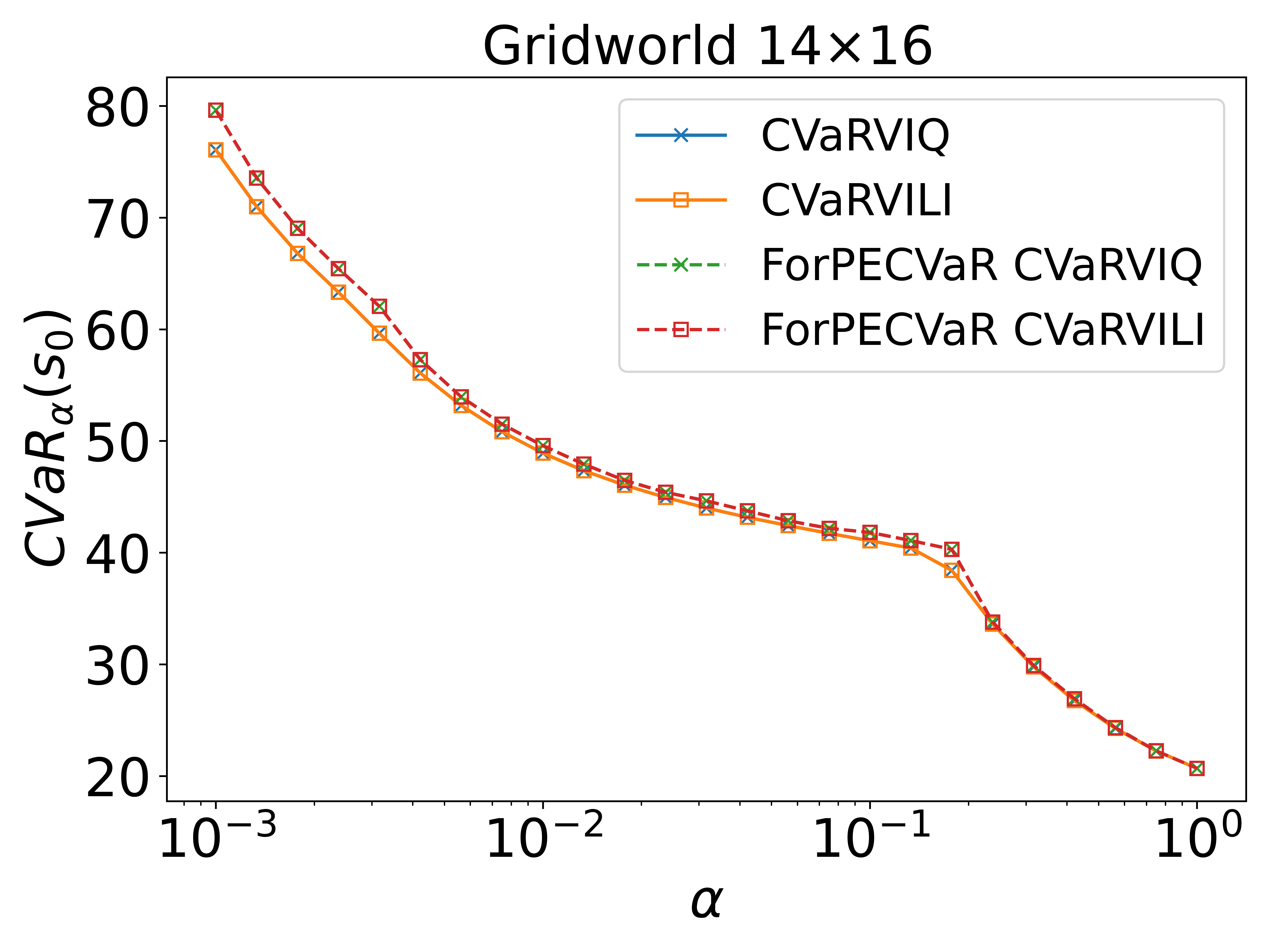
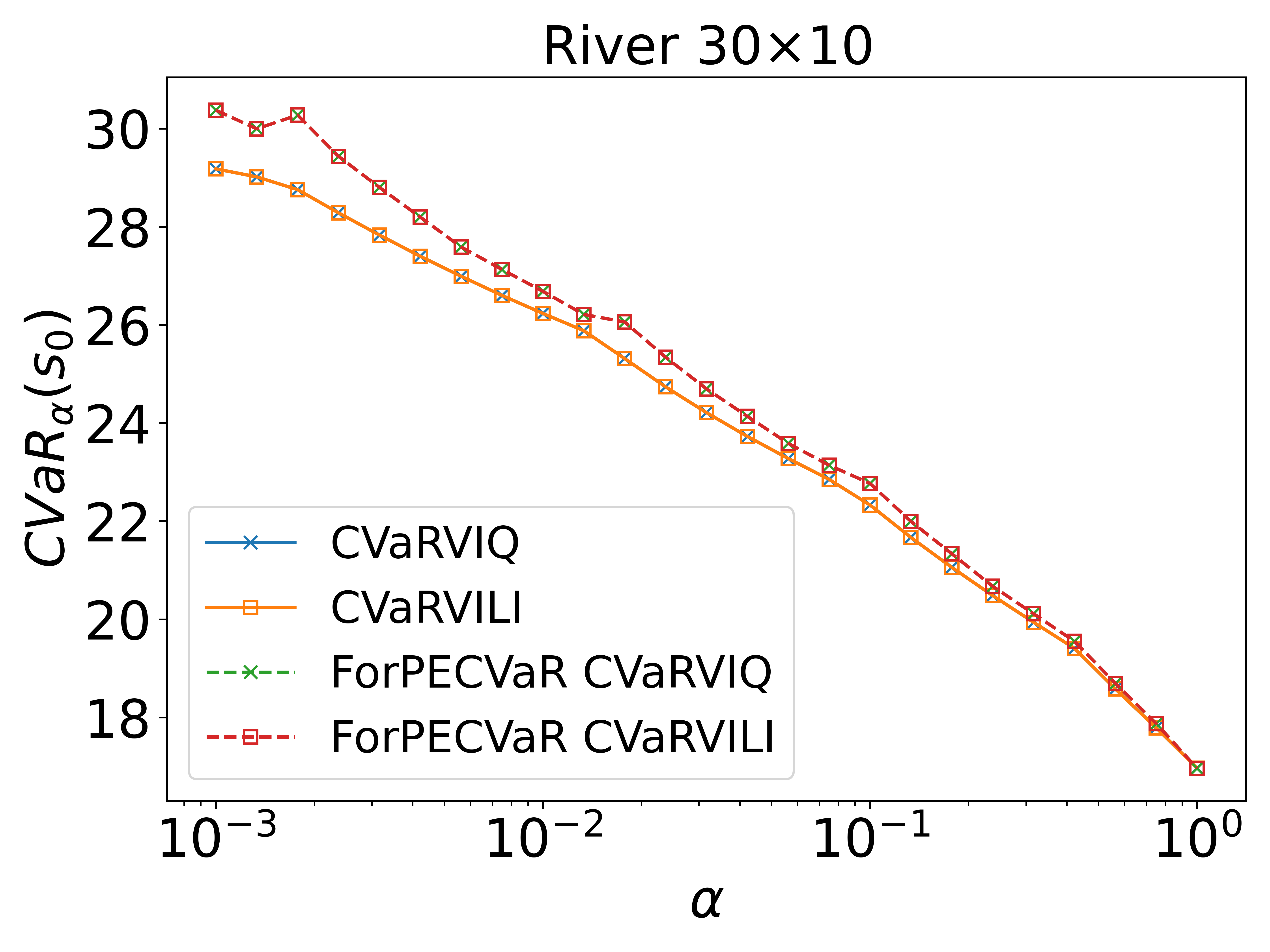
Figure 1. Approximate and exact values with $\displaystyle\alpha_{0}=10^{-3}$ and $\displaystyle|Y|=30$.

Fig. 2 shows the runtime in seconds for the Gridworld $\displaystyle 14\times 16$ and the River $\displaystyle 30\times 10$ problems for different settings varying $\displaystyle\alpha_{0}$ and $\displaystyle|Y|$. The figure shows that with more atoms it takes longer to solve the problem. The value of $\displaystyle\alpha_{0}$ influences the execution time, but to a lesser extent than the number of atoms. The results of the other problems are similar.

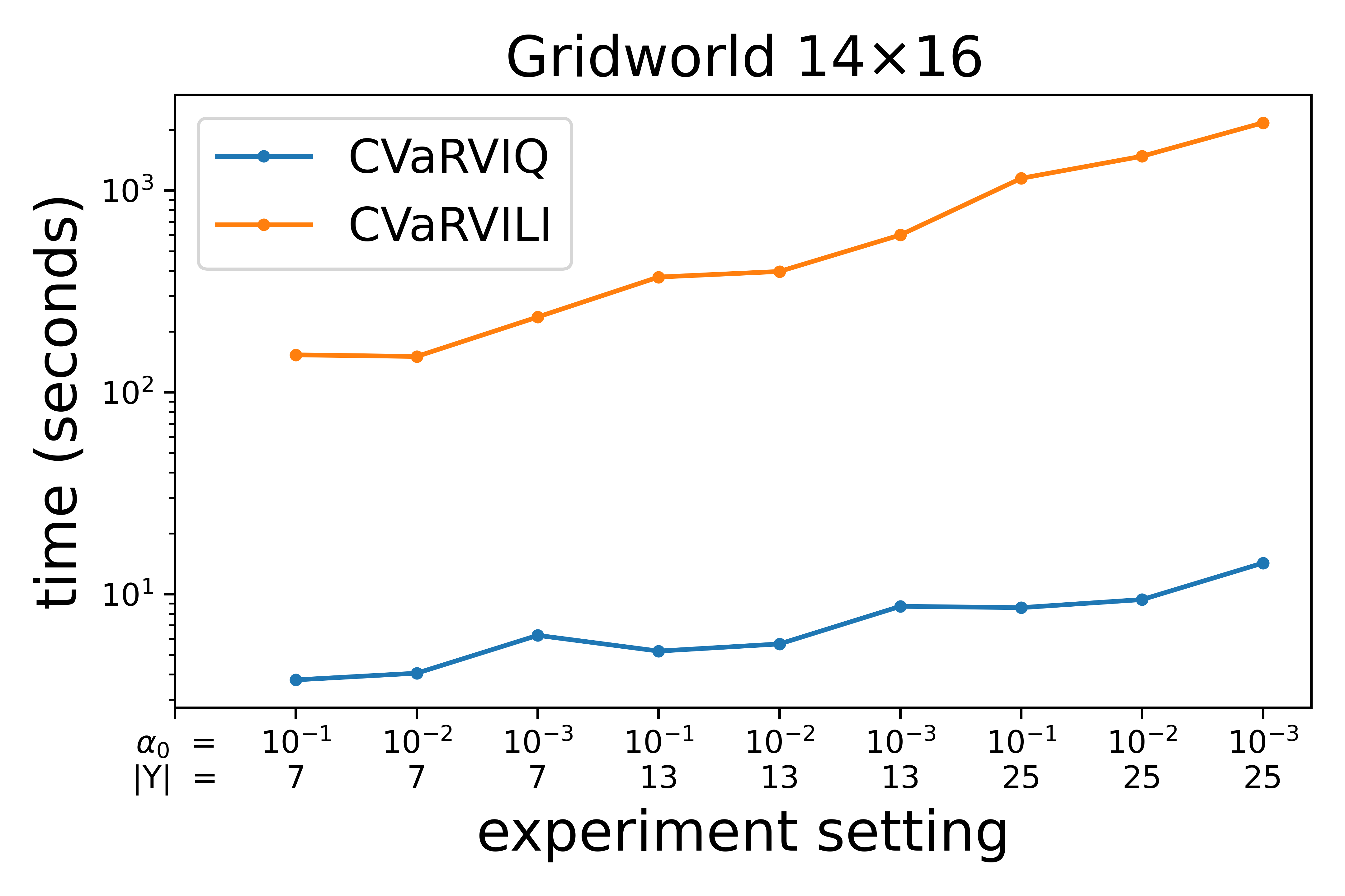
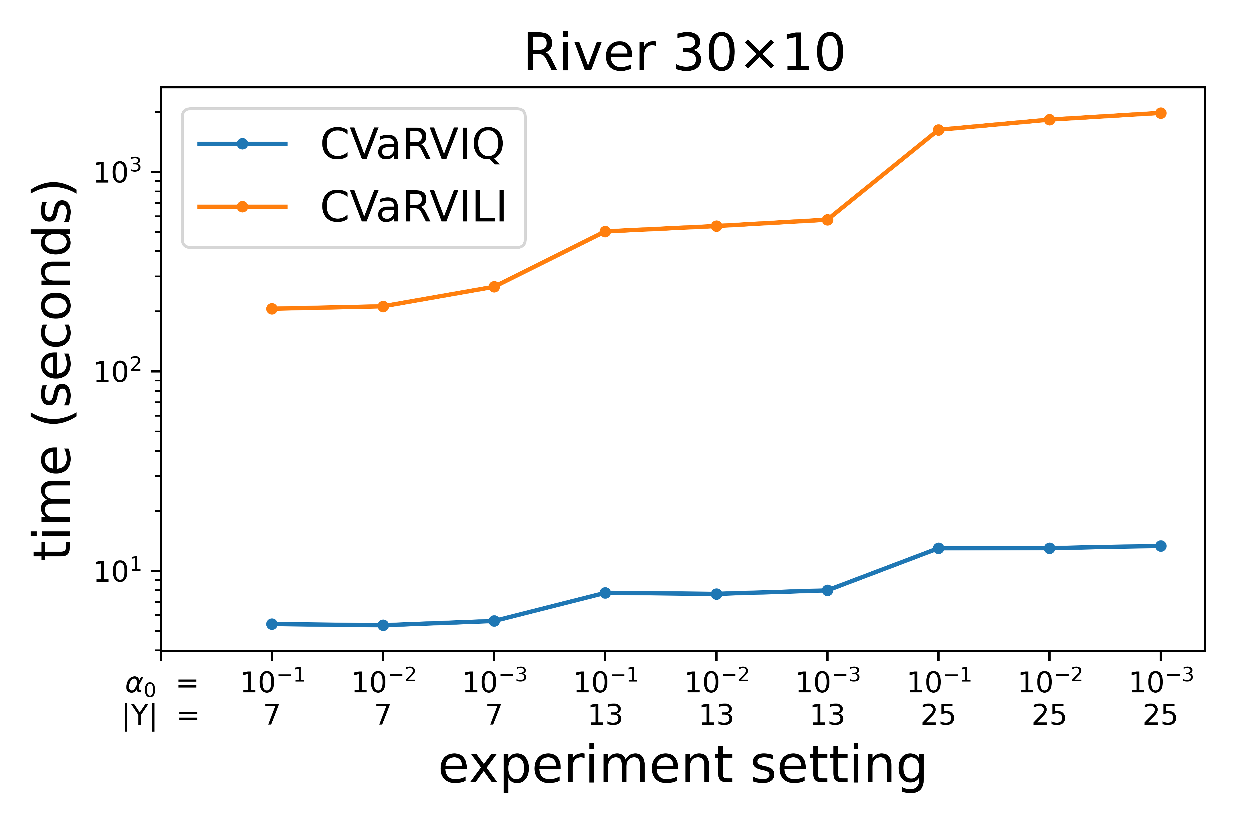
Figure 2. Execution time of CVaRVIQ and CVaRVILI.

Next, we analyze the influence of CVaRVIQ’s parameters on the quality of its solutions through two experiments. In the first one, we fixed the parameter $\displaystyle\alpha_{0}$ and varied $\displaystyle|Y|$. In the second one, we fixed the parameter $\displaystyle|Y|$ and varied the $\displaystyle\alpha_{0}$ values. The analysis is done only for the CVaRVIQ algorithm, since both algorithms have similar results in terms of quality, and the CVaRVIQ is more efficient than the CVaRVILI in terms of execution time.

4.2. Values of CVaRVIQ varying $\displaystyle|Y|$

Chow et al. Chow et al. (2015), in Theorem 7, show that the approximation error tends to be zero when the number of interpolation points is arbitrarily large by the application of the Interpolated Bellman operator. We believe that CVaRVIQ has the same behavior since the approximate values of both are similar in the experiments performed. We analyzed this by varying the parameter $\displaystyle|Y|$ with $\displaystyle\alpha_{0}$ fixed.

Fig. 3 shows the values for $\displaystyle\alpha_{0}=10^{-3}$ and $\displaystyle|Y|\in\{7,13,25\}$ for Gridworld $\displaystyle 14\times 16$ and River $\displaystyle 30\times 10$. The solid lines represent the approximate value found by CVaRVIQ and the dashed lines represent the policy evaluation of the CVaRVIQ policy using ForPECVaR. In Fig. 3 we can observe that with more atoms there is an increase in the approximate values and a decrease in the exact values so that the distance between approximate and exact values decreases, which is consistent with Theorem 7 of Chow et al. (2015). Considering all the experiments performed, the same behavior is observed. However, in general, points closer to $\displaystyle\alpha_{0}$ have a greater distance between approximate and exact values than points closer to $\displaystyle 1$.

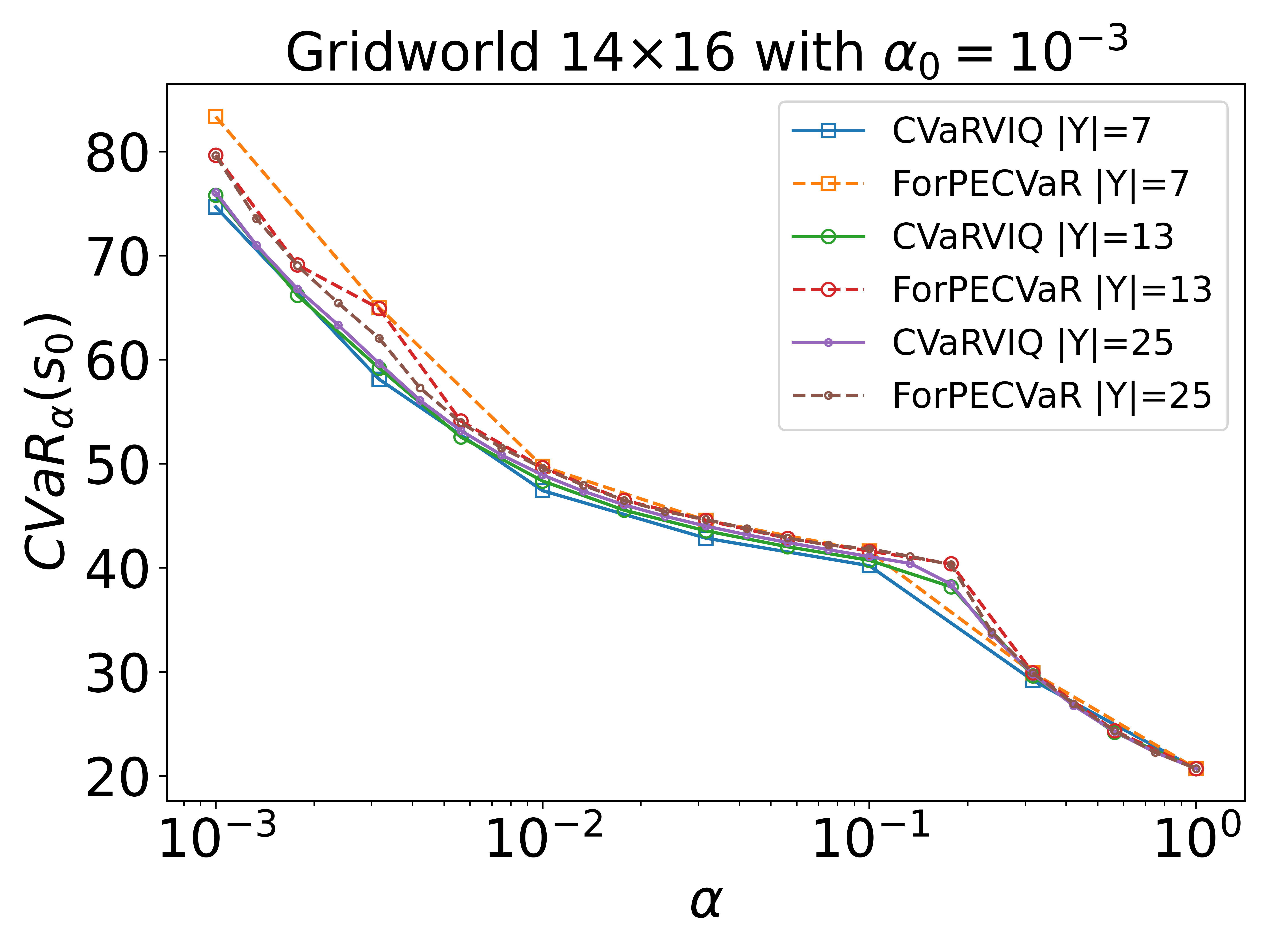
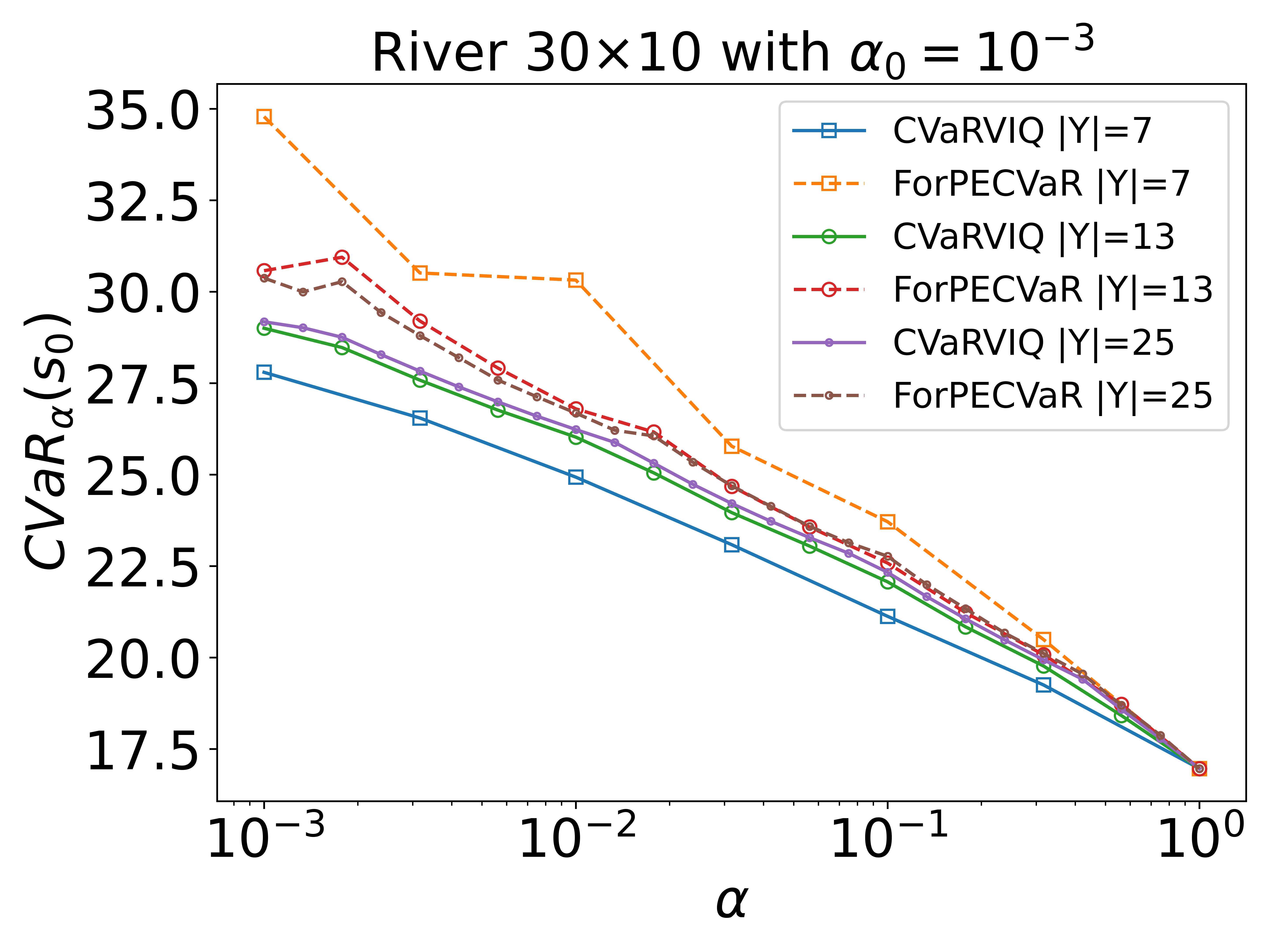
Figure 3. Approximate and exact values of CVaRVIQ varying the number of atoms with a fixed $\displaystyle\alpha_{0}$.

Fig. 4 shows the boxplots with the results of all experiments performed for $\displaystyle\alpha_{0}=10^{-3}$. Each boxplot has the values of the points of all experiments in the same domain with the same $\displaystyle\alpha_{0}$ and $\displaystyle|Y|$. The approximate values were normalized by the exact value in order to characterize the distance between them. Thus, normalized values closer to $\displaystyle 1$ correspond to a better approximation of the CVaRVIQ algorithm. Boxplots from experiments with fewer atoms have fewer points. For example, boxplots for $\displaystyle|Y|=7$ have 21 points (7 atoms for each of the 3 problems in each domain).

The boxplots show that the normalized values are closer to $\displaystyle 1$ with more atoms, i.e., approximations with few points produce worse policies, since the normalized value are farther from $\displaystyle 1$. Thus, we can observe that the value and policy of CVaRVIQ are moving toward the optimal value when using more atoms. The outliers in the boxplots correspond to experiments with atoms values closer to $\displaystyle\alpha_{0}$ regardless of the number of atoms used in the approximation. This happens because of a limitation of the approximate algorithms, which cannot approximate $\displaystyle\alpha_{0}$ well as observed in Section 4.3.

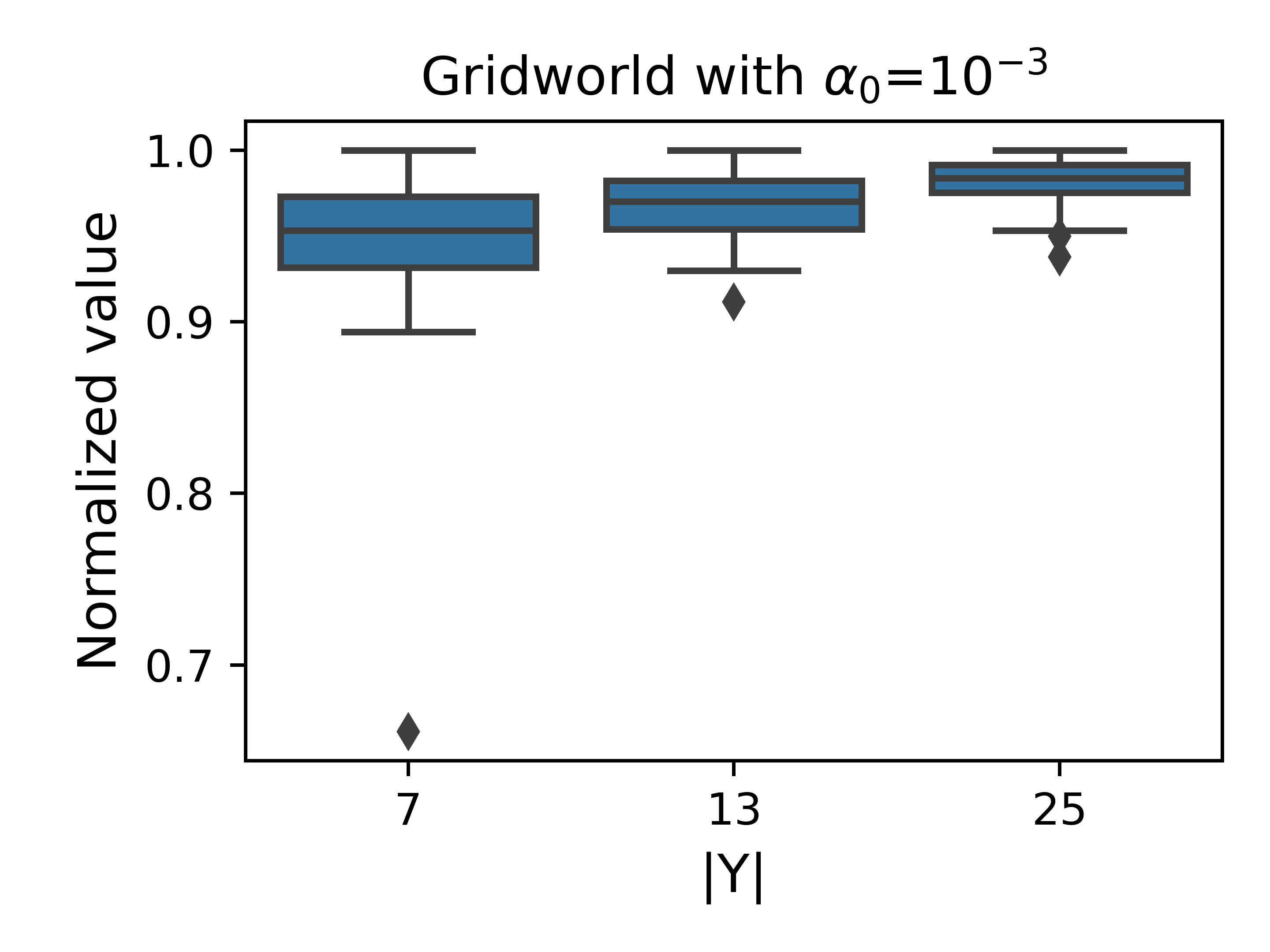
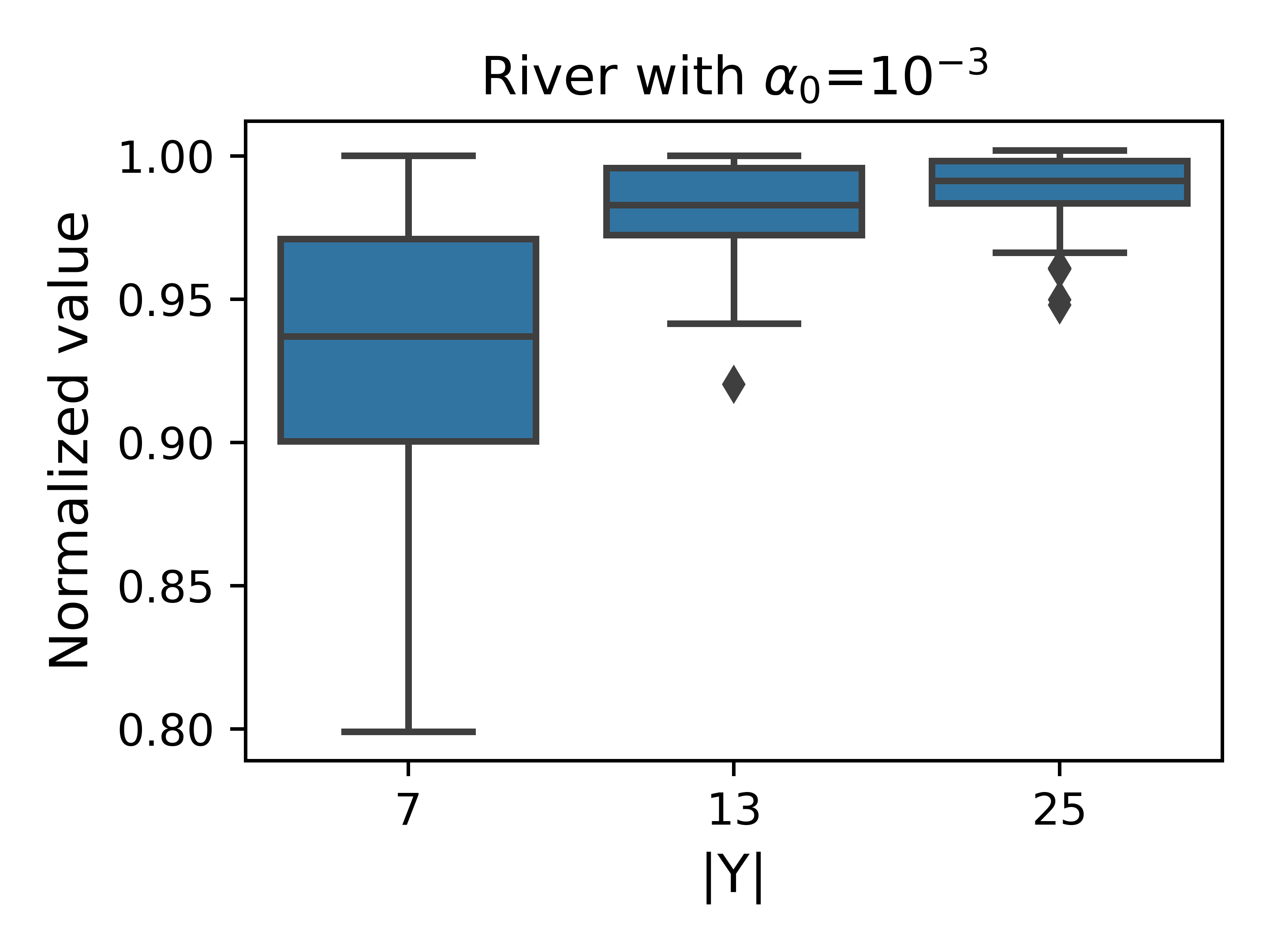
Figure 4. Boxplots with approximate values normalized by the exact values considering all problems of the Gridworld and River domains.

4.3. Values of CVaRVIQ varying $\displaystyle\alpha_{0}$

Since the distance between the approximate and exact values at $\displaystyle\alpha_{0}$ is substantial regardless of the number of atoms used, in this section, we investigate the use of an $\displaystyle\alpha_{0}$ smaller than the $\displaystyle\alpha_{target}$.

Fig. 5 shows the values of the experiments with $\displaystyle 25$ atoms for the Gridworld $\displaystyle 14\times 16$ and River $\displaystyle 30\times 10$ problems, both varying $\displaystyle\alpha_{0}\in\{10^{-3},10^{-2},10^{-1}\}$. In the Gridworld problem, for $\displaystyle\alpha=10^{-2}$, the exact value for the experiment with $\displaystyle\alpha_{0}=10^{-3}$ (orange line) is smaller than the value for the experiment with $\displaystyle\alpha_{0}=10^{-2}$ (red line). Analogously, for $\displaystyle\alpha=10^{-1}$, the exact values considering the experiments with $\displaystyle\alpha_{0}=10^{-3}$ and $\displaystyle\alpha_{0}=10^{-2}$ are better than with $\displaystyle\alpha_{0}=10^{-1}$. In the River problem, the same behavior does not happen, i.e., the exact value for the experiment with $\displaystyle\alpha_{0}=10^{-3}$ (orange line) is not smaller than the value for the experiment with $\displaystyle\alpha_{0}=10^{-2}$ (red line). This happen because the number of approximation points was not enough for obtaining a good solution. However, considering more atoms, the behavior is similar to the Gridworld results.

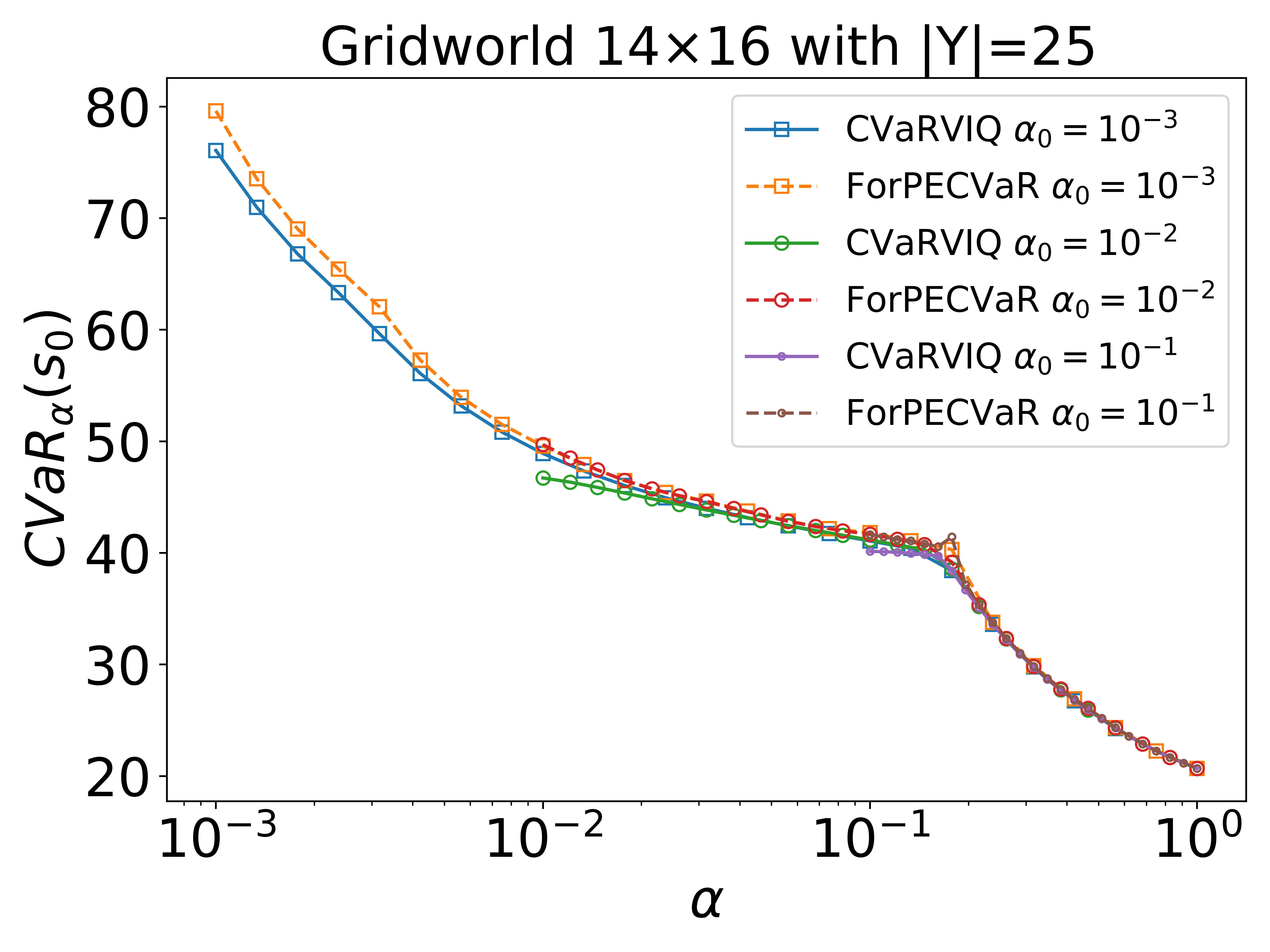
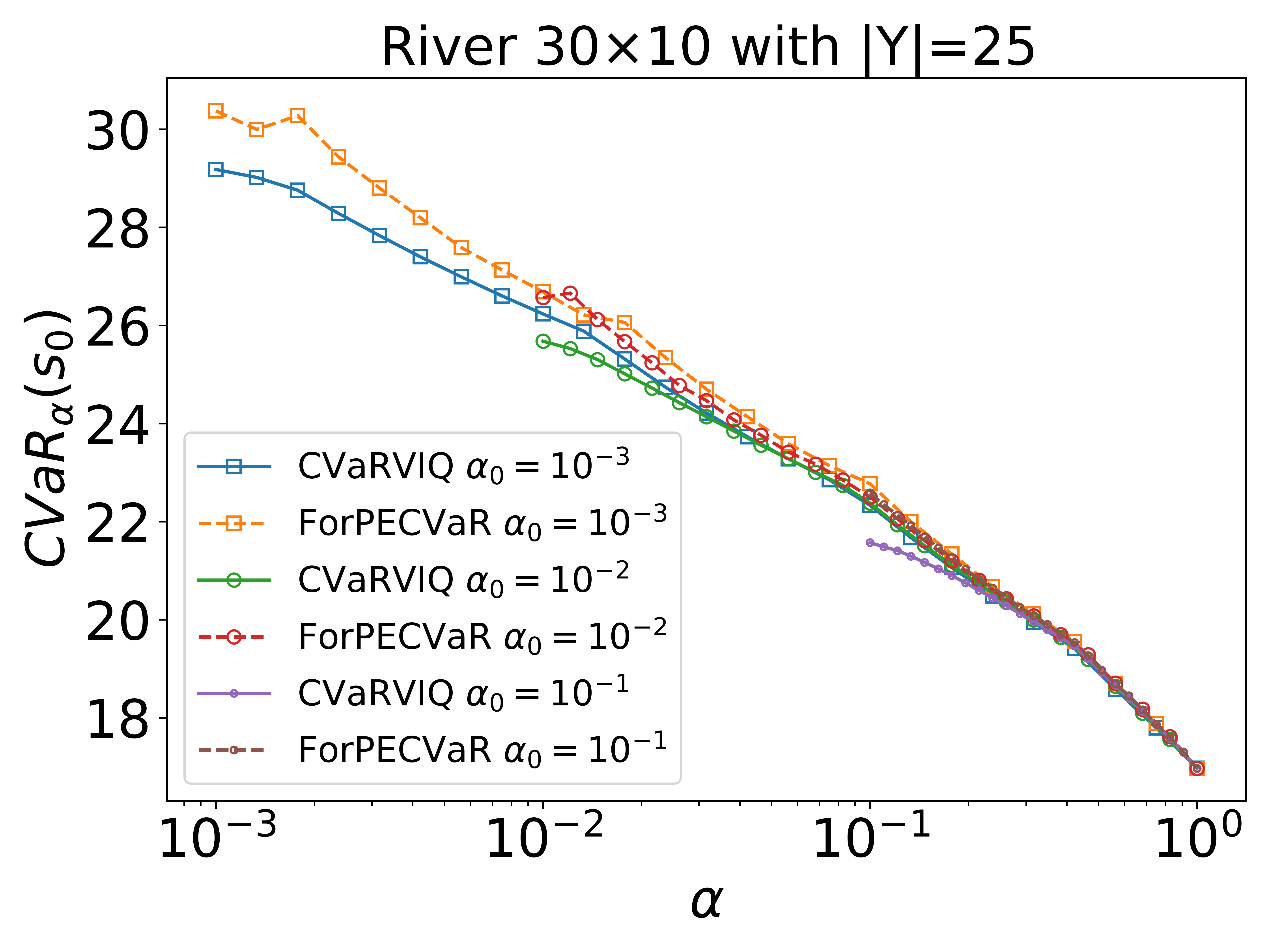
Figure 5. Approximate and exact values of CVaRVIQ varying the $\displaystyle\alpha_{0}$ values with a fixed $\displaystyle|Y|$.

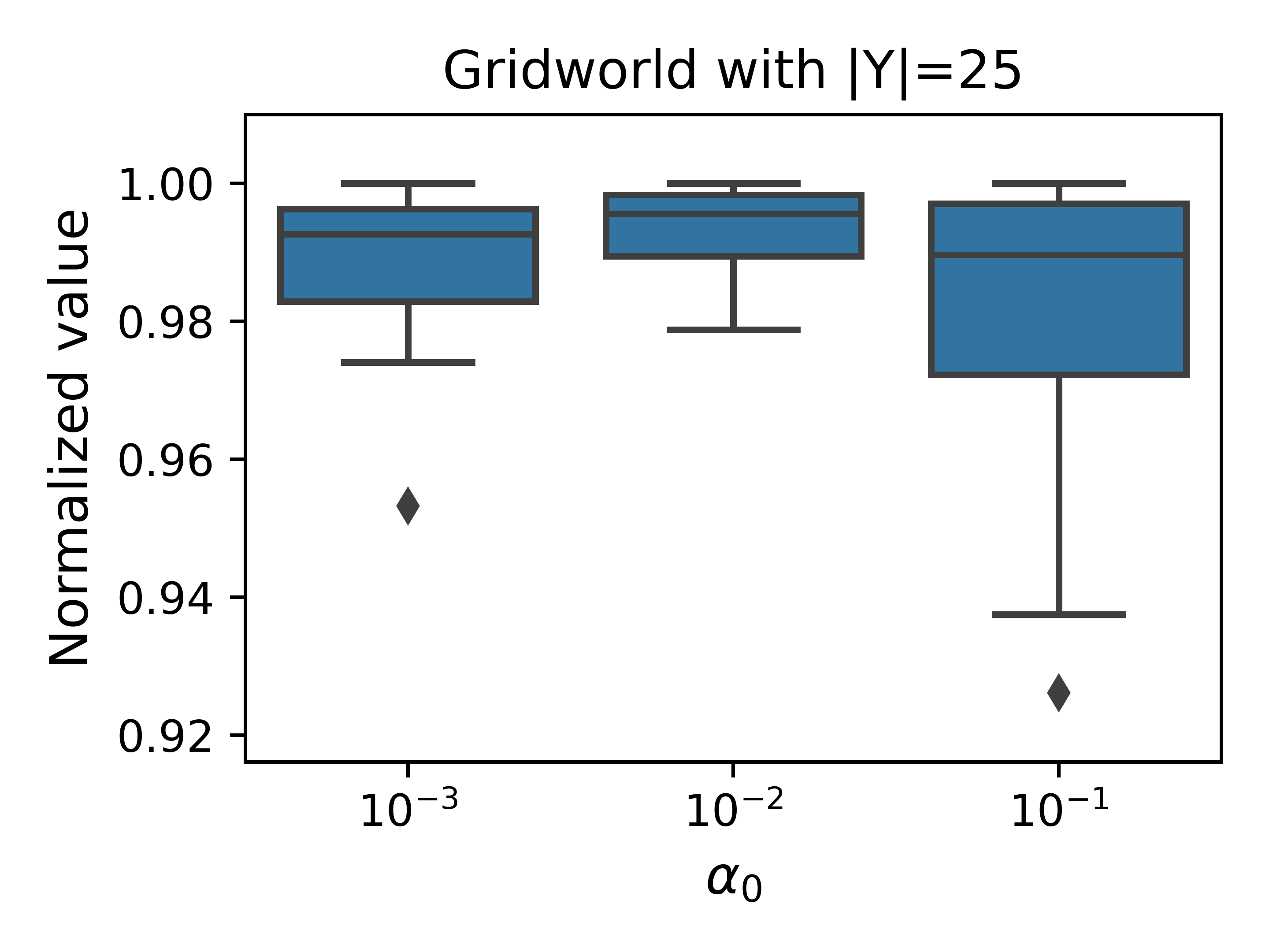
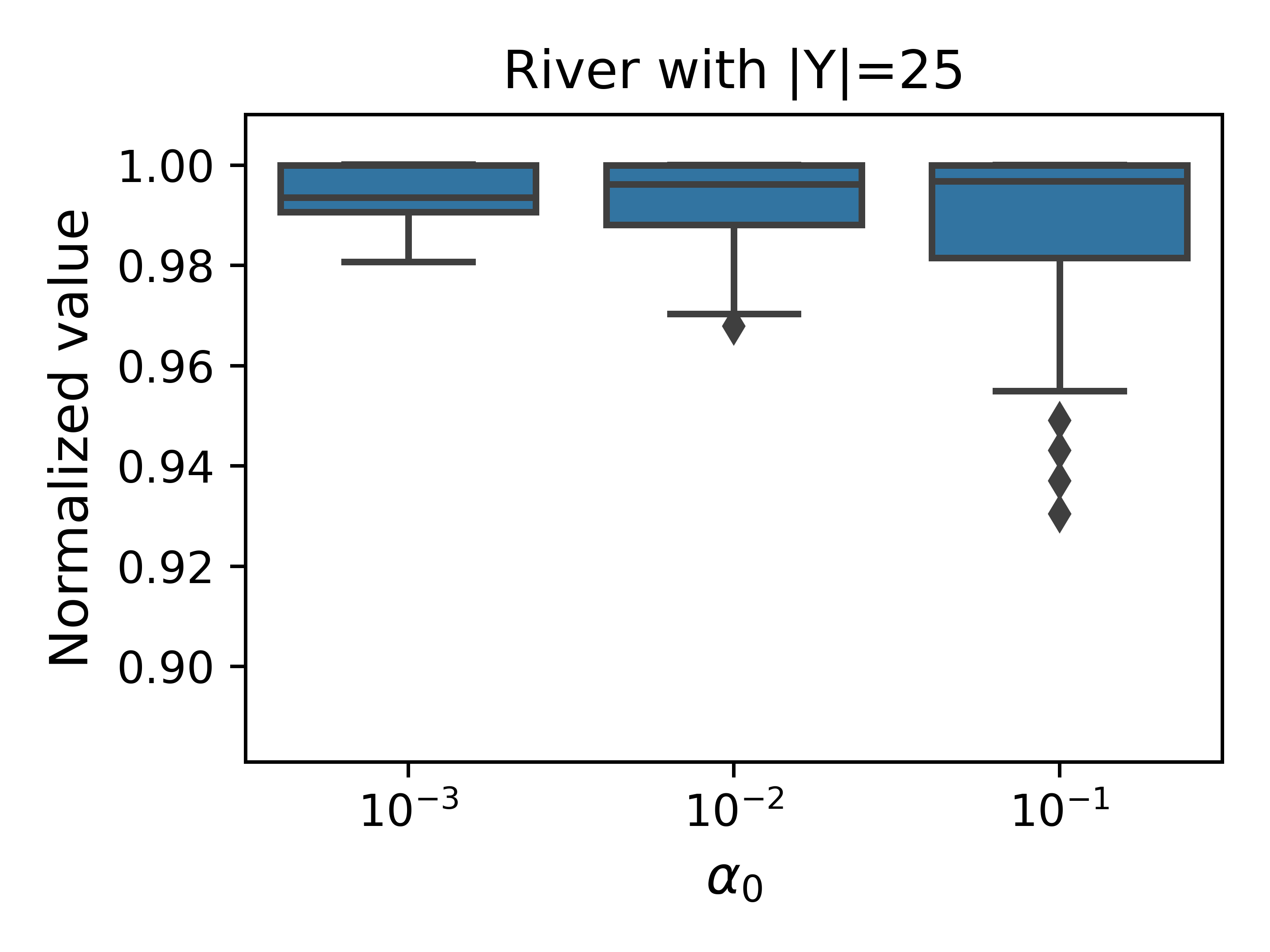
Figure 6. Boxplots with approximate values normalized by the exact values considering all problems of the Gridworld and River domains.

The boxplots in Fig. 6 show the approximate values normalized to the exact values for $\displaystyle\alpha_{target}=10^{-1}$. For each one of the $\displaystyle\alpha_{0}$, we selected the points of the respective $\displaystyle Y$ as $\displaystyle\widetilde{Y}=\{y|y\in Y\wedge y\geq\alpha_{target}\}$ where $\displaystyle y_{1}\in Y$ is equal to $\displaystyle\alpha_{0}$. Note that for each $\displaystyle\alpha_{0}$ different points could be selected. All points of each boxplot have the values of the experiments with the same $\displaystyle|Y|$ and $\displaystyle\alpha_{0}$ parameters. The experiments show that using a small number of atoms, $\displaystyle|Y|=7$ for example (boxplots not displayed because of the limit of space), the approximate values are far from the exact one. So first we can choose a suitable value of $\displaystyle|Y|$ (in these experiments it is better to choose 25). By setting $\displaystyle|Y|=25$, Fig. 6 shows that to choose an appropriate value of $\displaystyle\alpha_{0}$ to approximate $\displaystyle\alpha_{target}$, it is necessary to choose a value not too close from $\displaystyle\alpha_{target}$.

In the Gridworld and River domains, if we consider $\displaystyle\alpha_{0}=\alpha_{target}=10^{-1}$ and $\displaystyle|Y|=25$, the minimum normalized value and the first quartile is worse than the other ones for other values of $\displaystyle\alpha_{0}$. In the Gridworld domain with $\displaystyle|Y|=25$, the first quartile for $\displaystyle\alpha_{0}=10^{-2}$ is better than the first quartile for $\displaystyle\alpha_{0}=10^{-3}$ and $\displaystyle\alpha_{0}=10^{-1}$. In the River domain with $\displaystyle|Y|=25$, the first quartile for $\displaystyle\alpha_{0}=10^{-3}$ is better than the others.

Summing up, to obtain a good approximation for a problem with $\displaystyle\alpha_{target}$, first, we need to choose an adequate number of atoms and then choose $\displaystyle\alpha_{0}$ that is smaller than $\displaystyle\alpha_{target}$.

4.4. Execution time of ForPECVaR

Fig. 7 shows the runtime of ForPECVaR evaluation of CVaRVILI and CVaRVIQ policies for Gridworld $\displaystyle 14\times 16$ and the River $\displaystyle 30\times 10$ problems in seconds for different settings varying $\displaystyle\alpha_{0}$ and $\displaystyle|Y|$ for the atom $\displaystyle\alpha_{target}=\alpha_{0}$. For all experiments for a fixed $\displaystyle|Y|$, the lower the $\displaystyle\alpha_{0}$, the longer it takes to evaluate the policy. This is because it is necessary to reach the goal state with a higher probability. When fixing $\displaystyle\alpha_{0}$, we see that with more atoms, the execution time is longer, because with more atoms, the approximation of the policy is better, and the policy will tend to take more safe actions, which will take more time to reach the goal state with the necessary probability.

The Monte Carlo simulation (MC) technique can be used to evaluate approximately policies. We run 5 times MC to evaluate each of the 18 policies that correspond to the configurations of Fig. 7 with the same time spent by ForPECVaR to evaluate the CVaRVIQ policy. We calculate the difference between exact values computed by ForPECVaR and approximated values computed by MC. The mean was 0.67 and the median was 0.27 for the Gridworld problem, and 0.45 and 0.23 for the River problem, respectively on average. The maximum difference was 11.82 for the Gridworld problem and 5.29 for the River problem on average. Thus, MC can not get accurate evaluations of the performance of the policies considering the same time spent by ForPECVaR.

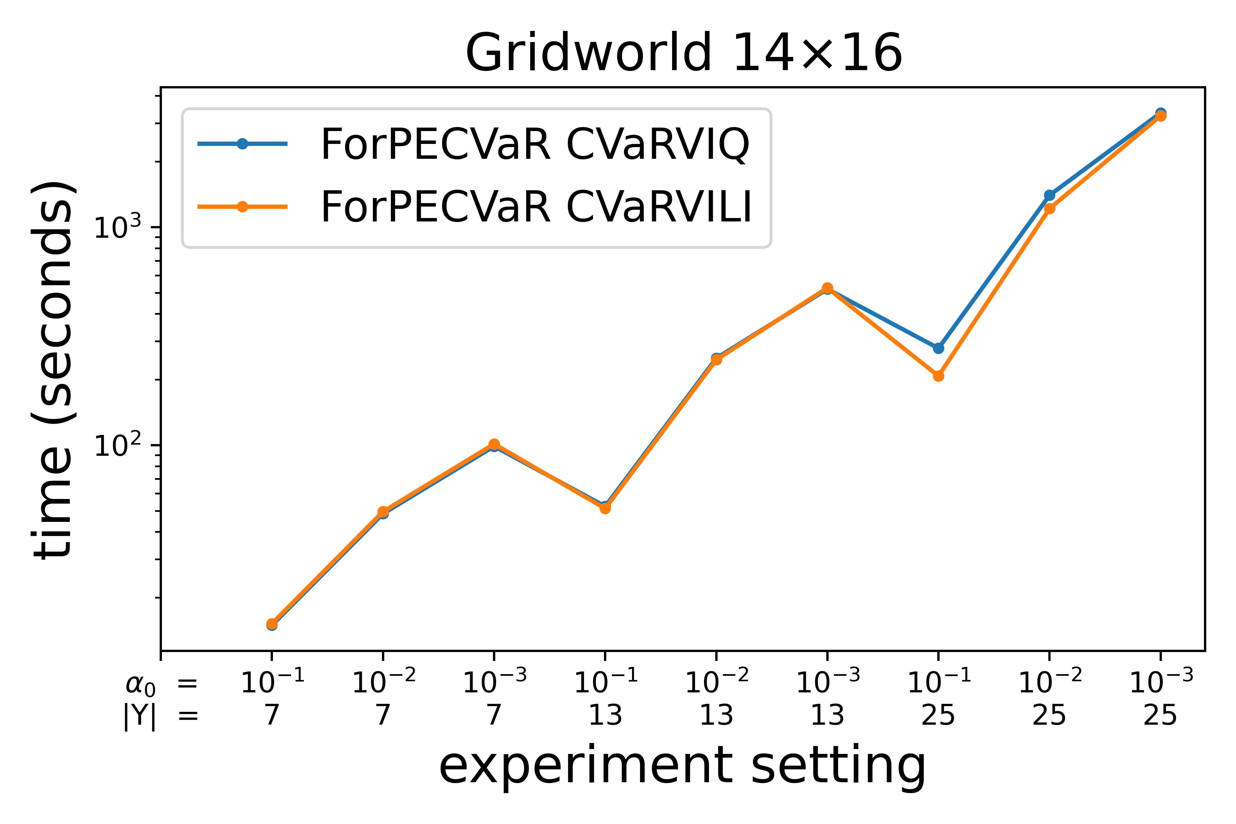
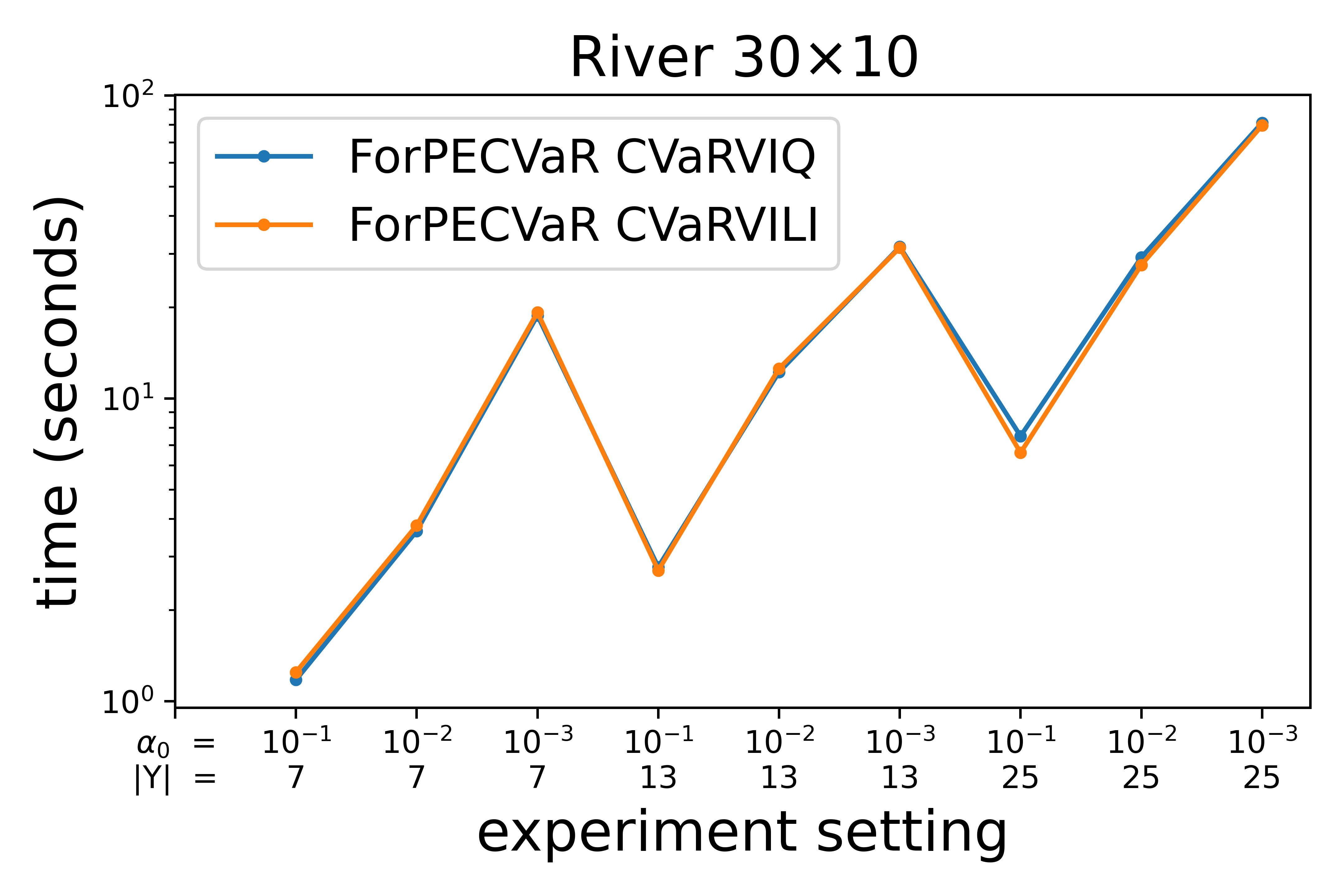
Figure 7. Execution time of ForPECVaR evaluation of CVaRVIQ and CVaRVILI policies for the atom $\displaystyle\alpha_{target}=\alpha_{0}$.

Table 1 shows the maximum execution time in seconds of ForPECVaR evaluation of CVaRVIQ and CVaRVILI policies for the atom $\displaystyle\alpha_{target}=\alpha_{0}$. In all cases, the execution time corresponds to the configuration of $\displaystyle|Y|=25$ and $\displaystyle\alpha_{0}=10^{-3}$, which are the highest number of atoms and the lowest confidence level tested. Gridworld problems policies have more execution time because the path toward the goal is longer than in the River problems, and more trajectories are expanded in the evaluation.

maximum time	Gridworld			River
(seconds)	$\displaystyle 5\times 5$	$\displaystyle 8\times 9$	$\displaystyle 14\times 16$	$\displaystyle 10\times 3$	$\displaystyle 16\times 6$	$\displaystyle 30\times 10$
CVaRVILI	6.79	122.52	3244.18	0.02	2.27	79.67
CVaRVIQ	7.95	130.12	3344.86	0.02	2.29	81.32

Table 1. Maximum execution time of ForPECVaR evaluation of CVaRVIQ and CVaRVILI policies for $\displaystyle\alpha_{target}=\alpha_{0}$.

5. Related Work

CVaRVILI finds an optimal approximate policy for CVaR MDP problems using linear interpolation. CVaRVIQ uses the connection between the $\displaystyle yCVaR_{y}$ and $\displaystyle VaR_{y}$ functions. The ForPECVaR algorithm is able to evaluate the policy returned by CVaRVILI and CVaRVIQ for problems with non-uniform costs. Meggendorfer Meggendorfer (2022) also proposed an algorithm to evaluate this type of policy. However, this algorithm only works for problems with uniform cost. Additionally, the code is not available and no experiments with this algorithm were performed in Meggendorfer (2022). ForPECVaR differs from this algorithm because the computed equations are different and it tracks the accumulated cost for each trajectory from the initial state independently. Each trajectory is added to a priority queue with respect to the accumulated cost and a heuristic can be used to improve the execution time of the algorithm. Recently, a Value Iteration based algorithm was proposed to find the optimal value of CVaR-SSPs Meggendorfer (2022). Note that these algorithms proposed in Meggendorfer (2022) were independently developed from our proposal.

Rigter et al. Rigter et al. (2022) formulate a lexicographic optimization problem that extends CVaRVILI and minimizes the expected cost subject to the constraint that the CVaR of the total cost is optimal. They show that there are multiple policies that get the same optimal CVaR value. However, they need the VaR value in their lexicographic approach that is obtained through MC simulations of the optimal CVaR policy in their experiments. ForPECVaR algorithm can be used by this algorithm since it also returns the exact VaR value. In Carpin et al. (2016) is defined a surrogate MDP problem to model a CVaR in the transient total cost MDP (similar to SSP). The solution to this problem approximates the optimal policy.

The CVaR criterion was also studied in the risk-sensitive reinforcement learning (RL) area Chow and Ghavamzadeh (2014); Chow et al. (2018); Tamar et al. (2015); Prashanth (2014); Stanko and Macek (2019); Keramati et al. (2020); Tang et al. (2020). Our proposal does not evaluate these policies as it needs state transitions to assess them. Another way to consider the CVaR criterion is through the use of constrained MDPs problems that considers a user-defined CVaR threshold as a constraint of an expected value optimization problem Chow and Ghavamzadeh (2014); Borkar and Jain (2014); Prashanth (2014); Chow et al. (2018). Rigter et al. (2022). The policies found with the CVaR-constrained problems can also be evaluated by ForPECVaR as long as the transitions of the model are known.

6. Conclusion

Given the existence of many algorithms with approximation to solve CVaR MDPs problems, it is important to have exact algorithms to evaluate them and the influence of their parameters. In this paper, we have presented ForPECVaR, an exact algorithm to evaluate any CVaR policy with a forward approach. In addition to the CVaR value, ForPECVaR also calculates the exact VaR value of the policies that can be used by other algorithms such as the algorithm proposed in Rigter et al. (2022). Our experimental evaluation has demonstrated that the approximate algorithms CVaRVILI and CVaRVIQ return similar policies and values, but the second has a better execution time. The exact evaluation of the CVaRVIQ policy shows a limitation of the algorithms analyzed in relation to the approximation of the values and policies closest to the minimum confidence level $\displaystyle\alpha$. We also showed that the simple approach of MC can not get accurate evaluations of policies considering the same time used by ForPECVaR.

References

- (1)
- Bäuerle and Ott (2011) Nicole Bäuerle and Jonathan Ott. 2011. Markov decision processes with average-value-at-risk criteria. Mathematical Methods of Operations Research 74, 3 (2011), 361–379.
- Bellemare et al. (2017) Marc G Bellemare, Will Dabney, and Rémi Munos. 2017. A distributional perspective on reinforcement learning. In International Conference on Machine Learning. PMLR, 449–458.
- Bertsekas and Tsitsiklis (1991) Dimitri P Bertsekas and John N Tsitsiklis. 1991. An analysis of stochastic shortest path problems. Mathematics of Operations Research 16, 3 (Aug. 1991), 580–595.
- Borkar and Jain (2014) Vivek Borkar and Rahul Jain. 2014. Risk-constrained Markov decision processes. IEEE Trans. Automat. Control 59, 9 (2014), 2574–2579.
- Carpin et al. (2016) Stefano Carpin, Yin-Lam Chow, and Marco Pavone. 2016. Risk Aversion in Finite Markov Decision Processes Using Total Cost Criteria and Average Value at Risk. In 2016 IEEE International Conference on Robotics and Automation (ICRA) (Stockholm, Sweden). IEEE Press, 335–342.
- Chow and Ghavamzadeh (2014) Yinlam Chow and Mohammad Ghavamzadeh. 2014. Algorithms for CVaR optimization in MDPs. In Proceedings of the 27th International Conference on Neural Information Processing Systems - Volume 2 (Montreal, Canada) (NIPS’14). MIT Press, Cambridge, MA, USA, 3509–3517.
- Chow et al. (2018) Yinlam Chow, Mohammad Ghavamzadeh, Lucas Janson, and Marco Pavone. 2018. Risk-Constrained Reinforcement Learning with Percentile Risk Criteria. Journal of Machine Learning Research 18 (2018), 1–51.
- Chow et al. (2015) Yinlam Chow, Aviv Tamar, Shie Mannor, and Marco Pavone. 2015. Risk-Sensitive and Robust Decision-Making: a CVaR Optimization Approach. In NIPS. 1522–1530.
- Freire and Delgado (2017) Valdinei Freire and Karina Valdivia Delgado. 2017. GUBS: A Utility-Based Semantic for Goal-Directed Markov Decision Processes. In Proceedings of the 16th Conference on Autonomous Agents and MultiAgent Systems (AAMAS ’17). 741–749.
- Keramati et al. (2020) Ramtin Keramati, Christoph Dann, Alex Tamkin, and Emma Brunskill. 2020. Being optimistic to be conservative: Quickly learning a CVaR policy. Proceedings of the AAAI Conference on Artificial Intelligence 34, 04 (Apr. 2020), 4436–4443.
- Meggendorfer (2022) Tobias Meggendorfer. 2022. Risk-Aware Stochastic Shortest Path. In Thirty-Sixth AAAI Conference on Artificial Intelligence. AAAI Press, 9858–9867.
- Prashanth (2014) LA Prashanth. 2014. Policy gradients for CVaR-constrained MDPs. In International Conference on Algorithmic Learning Theory. Springer, 155–169.
- Puterman. (1994) M. L. Puterman. 1994. Markov Decision Processes: Discrete Stochastic Dynamic Programming. Wiley-Interscience, New York, NY.
- Rigter et al. (2022) Marc Rigter, Paul Duckworth, Bruno Lacerda, and Nick Hawes. 2022. Planning for Risk-Aversion and Expected Value in MDPs. Proceedings of the International Conference on Automated Planning and Scheduling 32, 1 (Jun. 2022), 307–315.
- Rockafellar and Uryasev (2002) R.Tyrrell Rockafellar and Stanislav Uryasev. 2002. Conditional value-at-risk for general loss distributions. Journal of Banking & Finance 26, 7 (2002), 1443–1471.
- Stanko and Macek (2019) Silvestr Stanko and Karel Macek. 2019. Risk-averse Distributional Reinforcement Learning: A CVaR Optimization Approach.. In IJCCI. 412–423.
- Tamar et al. (2015) Aviv Tamar, Yonatan Glassner, and Shie Mannor. 2015. Optimizing the CVaR via Sampling. In Proceedings of the Twenty-Ninth AAAI Conference on Artificial Intelligence (Austin, Texas) (AAAI’15). AAAI Press, 2993–2999.
- Tang et al. (2020) Yichuan Charlie Tang, Jian Zhang, and Ruslan Salakhutdinov. 2020. Worst Cases Policy Gradients. In Proceedings of the Conference on Robot Learning (Proceedings of Machine Learning Research, Vol. 100), Leslie Pack Kaelbling, Danica Kragic, and Komei Sugiura (Eds.). PMLR, 1078–1093.