Guided Graph Generation: Evaluation of Graph Generators in Terms of Network Statistics, and a New Algorithm

Abstract

We consider the problem of graph generation guided by network statistics, i.e., the generation of graphs which have given values of various numerical measures that characterize networks, such as the clustering coefficient and the number of cycles of given lengths. Algorithms for the generation of synthetic graphs are often based on graph growth models, i.e., rules of adding (and sometimes removing) nodes and edges to a graph that mimic the processes present in real-world networks. While such graph generators are desirable from a theoretical point of view, they are often only able to reproduce a narrow set of properties of real-world networks, resulting in graphs with otherwise unrealistic properties. In this article, we instead evaluate common graph generation algorithms at the task of reproducing the numerical statistics of real-world networks, such as the clustering coefficient, the degree assortativity, and the connectivity. We also propose an iterative algorithm, the Guided Graph Generator, based on a greedy-like procedure that recovers realistic values over a large number of commonly used graph statistics, while at the same time allowing an efficient implementation based on incremental updating of only a small number of subgraph counts. We show that the proposed algorithm outperforms previous graph generation algorithms in terms of the error in the reconstructed graphs for a large number of graph statistics such as the clustering coefficient, the assortativity, the mean node distance, and also evaluate the algorithm in terms of precision, speed of convergence and scalability, and compare it to previous graph generators and models. We also show that the proposed algorithm generates graphs with realistic degree distributions, graph spectra, clustering coefficient distributions, and distance distributions.

1 Introduction

The problem of graph generation is concerned with finding algorithms that generate graphs whose properties match those of real networks. In general, graph generators are made to be realistic in two ways: (1) by mimicking the temporal evolution seen in a given input graph, and (2) by reproducing statistical properties of a given input graph. The two approaches are connected in a nontrivial fashion: A realistic graph growth model should in principle lead to realistic structural graph properties. In practice however, only the simplest models allow this relationship to be derived in closed form, and a practical graph generation algorithm can then usually follow only one of both. Due to the simplicity of generating graphs edge by edge and node for node, a large number of graph generators are thus formulated to follow criterion (1), without being able to derive guarantees for criterion (2). As a result, most graph generators cannot be easily tuned to produce given graph statistics. For instance, while many graph generators have a parameter that controls the amount of clustering (e.g., the probability of forming a triangle), these parameters cannot be easily adjusted to result in a requested value of the clustering coefficient – making such algorithms unsuited for generating graphs with an exact value of the clustering coefficient. This situation becomes even more difficult when multiple numerical graph properties are considered simultaneously. As an example, to generate a graph with a given degree distribution and clustering coefficient, a popular strategy involves first generating a graph with the requested degree distribution (via random assignment of half-edges), and then exchanging individual edges (performing switches) in a way that does not change the degree distribution, but changes the clustering coefficient. These techniques can be extended to switches of more than four nodes, as done for instance by Bansal and colleagues (2009). These kinds of methods are, by their nature, not generalizable to arbitrary graph statistics, since individual switching moves are restricted to maintaining a small set of graph properties. Therefore, this article will evaluate graph generation algorithms in terms of their ability to generate graphs with given values of numerical graph properties, and propose a new graph generation algorithm (the Guided Graph Generator) designed to achieve this goal with a high precision. The algorithm presented in this article is incremental and greedy-like, and uses the principle that no graph statistic should be taken as fixed – as long as the graph as a whole becomes closer to its intended statistic values. We show that the Guided Graph Generator can generate graphs that match the requested properties very closely, outperforming previous algorithms by several orders of magnitude in terms of precision.

Generating graphs with given properties is a central problem in the area of complex network analysis and graph mining, and can be used for various purposes: (1) anonymizing a network: generating a network with similar properties to a given one, but in which details of the original network cannot be recovered, (2) sampling a network: generating a network smaller than a given network, but with otherwise similar properties; this allows one to apply computationally expensive network analysis methods to networks that would normally be too large, and (3) scalability testing: generating graphs larger than a given graph, for the purpose of testing the scalability of a given network analysis method. Thus, it is no surprise that many different graph generators have been investigated, and that an algorithm for generating graphs that match the properties of real-world graphs well is an important goal. In all three cases, it is also true that generating graphs with precise values of the statistics is more important than having realistically designed steps of the algorithm, since in most cases only the final output of these algorithms is used. In this paper, we therefore propose a graph generation algorithm based on the idea of matching the value of numerical statistics: The graphs it generates have the same statistic values as any given input graph. This means that the proposed algorithm has the desirable property of having a very small parameter space. Nevertheless, it is able to reproduce given statistic values to a very high precision, so high in fact that, as we will see, other properties of the graph are also reproduced faithfully. Another concern with graph models is tractability: While graph models based on arbitrary numerical statistics exist (i.e., exponential random graph models, which represent one generic solution to the problem presented in this paper), the resulting fitting and graph generation algorithms are non-scalable to the point of being unused in practice for large graphs. The algorithm presented here has no such limitation, as an efficient method for vectorizing its calculations is available.

We start the paper by reviewing graph statistics and graph models in Section 2, with a focus on deriving the graph statistics resulting from each model. Then, in Section 3, we state the proposed Guided Graph Generator algorithm. We evaluate the previously existing and the proposed algorithm in Section 4 in terms of precision, scalability, and ability to reproduce various characteristic graph distributions, as well as compare the convergence of the proposed algorithm to the behavior of the previously existing algorithms. In Section 5, we discuss the limitations of the approach, and conclude in Section 6.

2 Graph Generation

A synthetic graph, as opposed to a real-world graph, is a graph generated algorithmically. A survey of graph generation algorithms is given by Chakrabarti and Faloutsos (2006). Graph generation algorithms can have many orthogonal goals, not all of which are shared by our approach – in the following, we give a structured overview of such graph generation algorithms with a focus on how each relates to the statistics of the graphs it generates.

2.1 Graph Statistics

As used in this article, a network statistic is a numerical value that characterizes a network. Examples of network statistics are the number of nodes and the number of edges in a network, but also more complex measures such as the diameter and the clustering coefficient. Statistics are the basis of a very large class of network analysis methods; they can be used to compare networks, classify networks, detect anomalies in networks and for many other tasks. Network statistics are also used to map a network’s structure to a simple numerical space, in which many standard statistical methods can be applied. Thus, network statistics are essential for the analysis of almost all network types. All statistics considered in this article are real numbers.

By definition, any graph model reduces a graph to certain characteristics of a graph. These can be individual numbers, but also more complex structures such as complete distributions. This is the case for instance when considering the degree distribution of a graph, or the distribution of the eigenvalues of a specific graph matrix. Note that the reduction of a graph to a simpler space, such as that defined by individual numbers or distributions is inherent in the concept of graph model: Any graph model which would take the whole graph and reproduce it would not be a graph model anymore. Thus, it is crucial to the definition of a graph model that the graph be reduced to a simpler structure. As such, individual graph statistics represent the simplest possible way to model a graph. Note also that reducing a graph to individual numbers is hardly restrictive: Almost all aspects of network analysis have been expressed as graph statistics, such as the clustering coefficient for measuring the clustering in a graph, the degree assortativity for measuring the assortativity, etc. Furthermore, more complex properties such as graph spectra can themselves be reduced to individual graph statistics, for instance by considering individual eigenvalues or moments of given distributions. As an example, the classical algebraic connectivity of graphs as defined by Fiedler (1973) equals the second smallest eigenvalue of a graph’s Laplacian matrix.

2.2 Random Graph Models

Synthetic graph generation is related to the concept of random graph models. In the simplest formulation, a random graph model is a probability distribution over all graphs with a given number of nodes. Random graph models can be specified by giving the probability of a graph, as is done with the Erdős–Rényi model (1959) and exponential random graph models (Robins et al., 2007), or can be specified by a randomized algorithm, such as the preferential attachment model of Barabási and Albert (1999). In the latter case, a random graph model can serve as a synthetic graph generator. Note that a random graph model specified as a probability distribution can be turned into a generative algorithm by using probabilistic algorithms such as Gibbs sampling. In general, the purpose of random graph models is to explain the mechanisms underlying the structure of real-world graphs, and as such the study of random graph models is tied to the theories (sociological or otherwise) explaining the structure of the graph. By contrast, other graph generators have the goal of reproducing the structures observed in real-world graphs, without however explaining them. Therefore, random graph models are usually only valid on those graphs for which the underlying theory is correct, and therefore random graph models are as a rule not evaluated by how many different graph datasets they are able to explain, as it is to be expected that different real-world networks have different underlying mechanisms of evolution. By contrast, the algorithms presented in this paper will be formulated as graph generators, i.e., with the goal to reproduce real-world graphs from many different areas, and therefore our approach does not explain any particular underlying graph creation mechanism, but produces synthetic graphs with characteristics matching many of them.

In addition to the number of nodes, which is usually taken as fixed, many different graph properties exist, and thus many different graph generation algorithms have been devised, each optimizing for one or more specific graph properties. The first and prototypical random graph model is the one of Erdős and Rényi (1959), which produces graphs in which the number of edges has a given expected value. While the Erdős–Rényi model was not intended to generate realistic graphs, it can be interpreted as the first of a series of graph models in which one or more graph properties have given input values. The Erdős–Rényi model is conceptually and computationally simple, but produces graphs that are highly unrealistic – their degree distributions are Poisson distributions and thus have a thin tail instead of a heavy one as seen in real-world networks. However, the average degree and characteristic distance between nodes they produce are usually realistic. In the Erdős–Rényi model, the only structural parameter apart from the number of nodes $n$ is the individual edge probability $p$. The expected number of edges is then $m=p{n\choose 2}$. Thus, the value $p$ can be chosen specifically to generate graphs in which $m$ has a given expected value. The number of edges is unique in allowing such a derivation; even random graph models that fix only one specific other statistic do not usually allow such a closed-form expression.

2.3 Preservation of Degree Distributions

It has been observed many times that real-world networks have power-law-like degree distributions, much different from Erdős and Rényi’s Poisson degree distributions. Accordingly, many graph models attempt to reproduce this property. For instance, the model of Barabási and Albert (1999) has been defined to grow graphs according to the rule of preferential attachment, i.e., edges attach with preference to nodes of high degree. This indeed leads to graphs with power-law degree distributions. An alternative random graph model that reproduces realistic degree distributions is the configuration model, also known as the Molloy–Reed model (1995). This model produces a graph with the exact same degree distribution as the input graph, but otherwise randomly distributed edges (Chatterjee et al., 2011). A related model is that of Chung and Lu (2002), which generates graphs in which each node has an expected degree matching that of the input graph. Both of these algorithms have the property that they use the full degree distribution as their parameters, and thus their parameter space has size $O(n)$. Both these models fix the expected degree distribution and thus fix the statistics that depend fully on it: the number of $k$-stars for $k\geq 1$, which for $k=1$ gives the number of edges. A generalization of these is the dK model by Mahadevan and colleagues (2007), which for $k=2$ produces graphs not only with a given degree distribution, but with a given joint degree distribution, i.e., the two degrees of connected nodes have the correct expected distribution. This additionally fixes the assortativity coefficient (i.e., the Pearson correlation coefficient of the degree of connected nodes). Another generalization of the configuration model attempts to recreate subgraph count distributions by splitting each subgraph into hyperstubs, i.e., individual nodes of the subgraph with half-edges attached. These can then be distributed among the nodes, analogously to the configuration model (Newman, 2009; Miller, 2009; Ritchie et al., 2016).

2.4 Clustering

A property not reproduced by any of the above models is clustering, i.e., the property of real-world graphs to contain groups of nodes well connected between each other, but less well connected to the rest of the graph. Clustering can be measured by the number of triangles present in a network, or equivalently by the clustering coefficient which equals the number of triangles normalized by the number of incident edge pairs. Many methods exist to produce graphs with realistic clustering. For instance, the Watts–Strogatz model (1998) produces graphs with realistic clustering and diameter. As it was not created to generate realistic graphs per se, it has the property that it generates unrealistic degree distributions, like the Erdős–Rényi model. Other models generalize the Molloy–Reed or Chung–Lu models to incorporate clustering to the generated graphs, for instance the algorithm of Bansal et al. (2009), and that of Pfeiffer et al. (2012). The BTER model of Seshadhri and colleagues (2012) is intended to reproduce not only the overall clustering coefficient, but the distribution of the local clustering coefficient over all nodes. Other degree distribution-based algorithms with a clustering component are given by Ángeles Serrano and Boguñá (2005).

2.5 Matrix-based Methods

Another class of graph properties and related algorithms are based on algebraic graph theory. This leads to several graph models that generate a graph’s adjacency matrix from individual building blocks. Of note in that category is the Kronecker model (Leskovec et al., 2010), which builds up an adjacency matrix by applying the Kronecker matrix product recursively starting with a small initial matrix. This model is attractive in that it allows the size of parameter space to be varied – it equals the number of independent values in the model’s $k\times k$ initiator matrix.

2.6 Exponential Random Graph Models

Exponential random graph models (ERGMs, also called p* models, Robins et al., 2007) are a class of random graph distributions based on arbitrary numerical graph statistics. ERGMs are motivated as the maximum-entropy graph distributions with given expected values of individual statistics. In theory, they can generate graphs with any given properties. In practice, they need very inefficient Monte-Carlo Markov chain fitting algorithms, such that only very small graphs can be used as input (Goodreau, 2007); large graphs have not been generated by them. What is more, they often display pathological behavior, as existing fitting algorithms will often result in extremal values of parameters, necessitating the use of additional rules such as alternating families of subgraph counts (Snijders et al., 2006). The Erdős–Rényi model is a special case in which the number of edges has a given expected value, and is also the only case for undirected graphs in which a closed-form solution to the parameter fitting problem is known.

2.7 Other Models

Other models exist, with more or less specific goals to emulate particular patterns of graphs or graph growth. The Waxman model (1988) is one based on an underlying geometry, assigning locations in a two-dimensional space to nodes, and connecting them with probability a function of their distance. The model is used in the context of Internet topologies. As we want to apply the algorithms also to networks without an underlying geometry, we will not consider it in this paper. What is more, the model is not amenable to fitting the parameters to an observed graph.

2.8 Graph Generation Strategies

A strategy common to many graph generation algorithms consists in creating a graph with one specific property, and then modifying the graph only in ways that preserve this property, in order to optimize another property. As long as such moves are possible, any graph property can be in principle recreated. The algorithm of Bansal et al. (2009) is a typical example: it starts with a random network that has the correct degree distribution, and proceeds to make switches that preserve the degree distribution but change the number of triangles. Thus, it is able to produce a graph with the correct number of edges, $k$-stars and triangles. The distribution of certain graph statistics in such models has also been studied by Ying and Wu (2009). However, other statistics such as the number of squares will not be realistic with them. In order to take the number of squares into account, it would be necessary to find a series of switches that preserve both the degree distribution and the number of triangles – a task that becomes intractable with an increasing number of statistics considered. As we will show, the proposed Guided Graph Generator algorithm allows instead changes to any statistic at each step, as long as the overall error (measured using all required statistics) decreases.

Certain graph generation algorithms require as a first step to generate a graph whose numerical properties have values in certain given ranges; an example being the method of Tabourier et al. (2011). This first step is usually non-trivial, and in fact the proposed algorithm complements these algorithms in that they can be used as that first step. A related but distinct task is that of enumerating all graphs with a given exact property (Read, 1981); this problem only applies to very small graph sizes and is not considered by our method. A previous comparison of graph generators with respect to such strategies is given by Sala et al. (2010).

2.9 Multi-Algorithm Methods

Another type of graph generation model combines multiple graph generation algorithms by choosing the appropriate one based on the requested properties themselves. For instance, such a method would use a Monte-Carlo graph generator based on exponential random graphs when the generated graphs must have a high clustering coefficient, and fall back to a preferential attachment model when the clustering coefficient is to be low. An example of this type of algorithm is the GMSCN method by Motalleb et al. (2013). These types of algorithms are orthogonal to individual algorithms as evaluated in this paper, since both can be combined. The method for choosing an algorithm itself must then be trained with these algorithms, leading to a machine learning problem that necessitates a large number of input graphs with differing characteristics; this is not necessary however for the individual methods used in this paper. The approach taken by these methods contrasts with the approach taken by our method, which is able to generate synthetic graphs whose numerical properties cover a large range of possible values.

2.10 Parameter Space

Graph models can additionally be classified by the size of their parameter space. Assuming that all models generate graphs with a fixed number $n$ of nodes, graph models then differ in the number of parameters they take:

Models such as the Erdős–Rényi model and exponential random graph models take a small, constant number of parameters that can be interpreted as graph statistics. As an example, the Erdős–Rényi model can be understood to be parametrized by the number of nodes and edges. The Kronecker model, too, takes a small constant number of parameters, i.e. the components of the initial matrix. All these models have an $O(1)$-dimensional parameter space.

Models that reproduce the degree distribution have the degree distribution as a parameter, and thus their parameter space has dimension $O(n)$. This is also true for BTER, in which the clustering coefficient distribution serves as the parameter.

Other models use a $O(n^{2})$-dimensional parameter space, such as the method of Gutfraind et al. (2015), which starts with the actual input graph, and modifies it iteratively. Another class of algorithm with $O(n^{2})$-dimensional parameter space is given by algorithms that use the full eigenvalue decomposition of characteristic graph matrices such as the Laplacian matrix (Xiao & Hancock, 2006; White & Wilson, 2007). These models are rare and do not strictly fulfill the purpose of a graph generator, since for instance the input graph may not be completely anonymized with them. Also, such algorithms have the property that they could reproduce the original graph’s properties faithfully by not performing any changes at all. Thus, the goal of these algorithms is to simultaneously anonymize graphs and retain their characteristics. Due to their use of $O(n^{2})$ parameters, their purpose is distinct from that of the algorithms evaluated in this paper, whose challenge lies in recreating the original graph’s properties with only $O(1)$ parameters. The algorithm proposed in this paper has a parameter space consisting of seven real numbers (including the number of nodes), and thus belongs to the first class of algorithms, i.e. those with constant parameter size.

2.11 Measuring the Quality of a Graph Generation Algorithm

As used in this article, a network statistic is a numerical measure that characterizes a network. A graph generation algorithm can then be evaluated by comparing the network statistics of the graphs it generates with the requested values. In principle, we may use as an error measure any distance function based on these. In the evaluation of the different algorithms, we will use the squared differences between the produced statistic values and the target statistic values. In our experiments, the choice of whether to use the absolute value or the square did not result in significant variation of results. In order to avoid further parameters in our evaluation, we thus choose to weight each statistic equally, giving a parsimonious error measure based on the squared differences between statistic values. Note also that a monotonous transformation of the error function does not result in a change of our evaluation, or, as we will see, in the output of the proposed algorithm.

Given an input graph $G_{0}$ and a generated graph $G$, we define the relative error with respect to a network statistic $S$ as

$$E^{S}=\frac{S(G)-S(G_{0})}{S(G_{0})}$$ (1)

in which $S(G)$ denotes the statistic value $S$ of the graph $G$. Based on the relative error, we then define the total error of an algorithm at generating a graph as

$$E=\left[\frac{1}{|\mathcal{S}|}\sum_{S\in\mathcal{S}}(E^{S})^{2}\right]^{1/2},$$ (2)

where $\mathcal{S}$ is the set of considered network statistics. The factor $1/|\mathcal{S}|$ ensures that $E$ is the root mean squared relative error of all relative errors. In the next section, we describe the proposed Guided Graph Generator for minimizing this value $E$, and then compare the previously described baseline algorithms with the proposed one in the subsequent section.

3 The Guided Graph Generator

We are now ready to describe the Guided Graph Generator, an algorithm we propose to generate graphs with precise values of given network statistics. The algorithm is iterative; it starts with a network that has the requested number of nodes $n$, and continues to modify the network step by step to bring its graph statistics nearer to those of the input graph. The algorithm is parametrized by a set of graph statistics $\mathcal{S}$ which must be chosen when the algorithm is run – we first describe the algorithm in terms of that choice, and then discuss the choice in the next section. Note that $\mathcal{S}$ represents the set of statistics, rather than statistic values; it merely encodes which graph statistics have been chosen. As opposed to related iterative graph generators such as that of Bansal et al. (2009), the proposed algorithm does not preserve the properties of the graph at each step. Instead, we allow changes in any property as long as the value of another property is made nearer to that of the input graph.

The input to the algorithm is a graph $G_{0}$ whose properties are to be replicated, as well as set of graph statistics $\mathcal{S}$. As noted earlier, $\mathcal{S}$ contains only information about the choice of which graph statistics are used, rather than individual values – those can be calculated from the given $G_{0}$. The proposed algorithm works by taking as a starting point an Erdős–Rényi graph with the correct number of nodes and edges, and then modifying the graph iteratively until the resulting graph is as close as possible to the target. To measure how close the generated graph is to the target graph, we use the error measure $E$ as defined in Equation (2) in the previous section. At each step of the iteration, we need to consider a certain number of possible changes in the graph, and choose the change which leads to the lowest error measure $E$. In order to compute the changes in the statistics efficiently, individual changes that are considered should be small, such that the changes in the statistic values can be easily computed. The smallest change that we can make in a graph (without changing the node set) is to add or remove an edge. In fact, the change in subgraph count statistics for the addition and removal of an edge can be expressed in terms of the immediate properties of the two involved nodes. Furthermore, in order to allow the algorithm to be optimized, the computation of the changes in statistics over all changes considered in one step should make use of common subexpressions whenever possible. Thus, we consider at each step the addition and removal of edges connected to one single node. As we show in the next section, this leads to efficient expressions for the change in subgraph count statistics, which leads to efficient expressions for computing $E$ at each step. We note that the described algorithm, while it performs the changes with best reduction in error at each step, is not a pure greedy algorithm, as it does not terminate once the error cannot be further reduced. The general form of the proposed Guided Graph Generator algorithm applying to any set of network statistics is given in Algorithm 1.

0:  a graph $G_{0}=(V,E_{0})$

0:  a set of statistics $\mathcal{S}$

0:  a convergence parameter $\epsilon>0$

0:  a graph $G=(V,E)$  

  $G=\textrm{ErdősRényi}(|V|,|E_{0}|/{|V|\choose 2})$

  for all $S\in\mathcal{S}$ do

     $x^{S}=S(G_{0})$

     $y^{S}=S(G)$

  end for

  repeat

     Choose a node $u\in V$ at random

     for all $S\in\mathcal{S}$ do

        for all $w\in V\setminus\{u\}$ do

           $\Delta^{S}_{w}=S(G\pm\{u,w\})-S(G)$

        end for

     end for

     $v=\mathrm{argmin}_{w\in V\setminus\{u\}}\sum_{S\in\mathcal{S}}((y^{S}+\Delta^{S}_{w}-x^{S})/x^{S})^{2}$

     $G=G\pm\{u,v\}$

     for all $S\in\mathcal{S}$ do

        $y^{S}=y^{S}+\Delta^{S}_{v}$

     end for

     $E^{\prime}=\sum_{S\in\mathcal{S}}((y^{S}-x^{S})/x^{S})^{2}$

  until $E^{\prime}$ has not attained a new minimum value in the last $(-|V|\log\epsilon)$ iterations

Algorithm 1 The proposed Guided Graph Generator algorithm in non-vectorized form, given for an arbitrary set of of graph statistics $\mathcal{S}$.

We use the following notation: the function $\textrm{ErdősRényi}(n,p)$ generates an Erdős–Rényi graph with $n$ vertices and edge probability $p$. $G\pm\{u,v\}$ denotes the graph $G$ in which the state of the edge $\{u,v\}$ has been switched, i.e., removed or added depending on whether $\{u,v\}$ is present or not. The convergence parameter $\epsilon$ ensures that the expected ratio of nodes $u$ that were not visited since the last new minimum value $E^{\prime}$ was found equals $\epsilon$. In all experiments, we use a value of $\epsilon=0.01$.

3.1 Choice of Graph Statistics

The Guided Graph Generator algorithm can in principle be applied to any numerical graph statistic such as the number of triangles, the graph diameter, or the degree assortativity. In practice, the choice of used graph statistics must be made such that they lead to efficient update algorithms, and are representative of important graph characteristics.

Updatability.

To result in an efficient update algorithm, we note that properties such as for example the graph diameter do not allow simple update expressions when the graph is modified. When an edge is added to a graph, we know that the diameter cannot increase, but to compute by how much it decreases (if at all), requires a computation almost as complex as the computation of the diameter in the first place. Therefore, global statistics such as the diameter are not suited to be used in the proposed algorithm. The same is true for graph statistics based on eigenvalues of characteristic graph matrices, such as the algebraic connectivity, or the spectral norm. Instead, we use statistics whose change depends linearly on local changes in the graph. These correspond to subgraph counts, i.e. the count of various subgraphs such as triangles. As another example, the number of 4-cliques (i.e., complete graphs $K_{4}$) does not allow a simple vectorial update expression, and is therefore not used.

Representativity.

At the same time, the chosen statistics should be representative of graph characteristics that are important in practice. For instance, the number of triangles $t$ forms the basis for the widely used clustering coefficient ($3t/s$); the number of edges $m$ determines the graph’s density ($2m/n$); and the number of squares, being the smallest possible even cycle when multiple edges are excluded, determines the bipartivity of the graph (Estrada & Rodríguez-Velázquez, 2005). The degree distribution, itself used as a parameter for graph models, is tightly related to the number of $k$-stars, which are related to its moments (Olbrich et al., 2010). A $k$-star is a pattern in which a central node is connected to $k$ other nodes. Thus, a 2-star is a wedge, a 3-star is a claw and a 4-star is a cross.

Interdependence of graph statistics.

Certain graph statistics are related to each other in mathematically precise ways. For instance, the clustering coefficient $c$, defined as the probability that two incident edges are completed by a third edge to form a triangle, can be expressed as $c=3t/s$, where $t$ is the number of triangles in the graph, and $s$ the number of wedges. Thus, the clustering coefficient, while not being a subgraph count statistic, can be recovered in graph models that optimize $t$ and $s$. Thus, while the algorithm presented in this paper does not explicitly optimize for $c$, it does so implicitly because it optimizes $t$ and $s$.

In total, we consider six simple possible graphs that are connected: the edge, the wedge, the triangle, the square, the claw and the cross. The complete list is given in Table 1. Note that the number of nodes $n$ is a constant in the algorithm, and is not modified. These six subgraphs cover all possible connected subgraphs up to three nodes, and those with more than three nodes for which an update is easily expressible. Other graph characteristics not covered by them such as the diameter or average path length will be subject to experiments in Section 4.

Table 1: The subgraph patterns optimized by the Guided Graph Generator algorithm presented in this paper, along with a selection of graph properties that are represented by each subgraph count.

Pattern Statistic Graph properties covered $m=$ volume, number of edges Density, community size $s=$ number of wedges/2/̄stars/2-paths Degree distribution, preferential attachment $z=$ number of claws/3-stars Degree distribution, preferential attachment $x=$ number of crosses/4/̄stars Degree distribution, preferential attachment $t=$ number of triangles/3/̄cycles/3-cliques Clustering, triangle closing, analysis of triads, small-world property $q=$ number of squares/4/̄cycles Bipartivity, clustering in bipartite and nearly-bipartite graphs

3.2 Fast Computation of $\Delta^{S}_{w}$

Algorithm 1 requires us to compute the difference in statistics between the current graph $G$ and the graph $G$ with one edge added or removed:

$$\Delta^{S}_{w} =S(G\pm\{u,w\})-S(G)$$

In order for the the Guided Graph Generator to be fast, this calculation must be performed in a vectorized way. The existence of closed-form expressions for $\Delta^{S}_{w}$ decides whether a particular statistic can be used in the proposed algorithm. Since $\Delta^{S}_{w}$ must be computed at each step for all nodes $w\in V$ (except for $w=v$), we derive vectorized expressions that give a vector $\Delta^{S}$ containing the value $\Delta^{S}_{w}$ for all $w\in V$. The individual value computed for $w=v$ is then simply ignored.

During the run of the algorithm, the graph $G$ is always represented by its symmetric adjacency matrix $\mathbf{A}\in\{0,1\}^{n\times n}$. We now give expressions for the vectors $\Delta^{S}$ measuring the change in statistic $S$ expressed as functions of $\mathbf{A}$, for each statistic $S\in\{m,s,z,x,t,q\}$. These expressions make use of the degree vector $\mathbf{d}$, which must be updated along with the matrix $\mathbf{A}$. $\mathbf{u}\circ\mathbf{v}$ will denote the entrywise product between two vectors $\mathbf{u}$ and $\mathbf{v}$, and $\mathbf{A}_{:u}$ the $u$-th column of $\mathbf{A}$. In the following, we note which operations make use of a matrix-vector product of size $n$, as these are the most expensive operations.

Number of edges $m$. The number of edges will always increase or decrease by one, depending on the previous state of the edge $\{u,w\}$.

$$\Delta^{m} =-2\mathbf{A}_{:u}+1$$

Number of wedges $s$. When adding an edge, the number of wedges increases by the sum of the degrees of the two connected nodes. When removing an edge, the number of wedges decreases by the sum of the degrees of the two nodes, minus two.

$$\Delta^{s} =\Delta^{m}\circ(\mathbf{d}+\mathbf{d}_{u})+2\mathbf{A}_{:u}$$

Number of claws $z$. When the two nodes $u$ and $w$ are not connected, the number of added claws equals $\mathbf{d}_{u}(\mathbf{d}_{u}-1)+\mathbf{d}_{w}(\mathbf{d}_{w}-1)$. When the two nodes are connected, the number of removed wedges can be computed in the same way, but based on the degrees after the removal.

$$\Delta^{z} =\frac{1}{2}\Delta^{m}\circ[(\mathbf{d}-\mathbf{A}_{:u})\circ(\mathbf{d}-1-\mathbf{A}_{:u})$$

$$\qquad\qquad\,\,\,\,\,+(-\mathbf{A}_{:u}+\mathbf{d}_{u})\circ(-\mathbf{A}_{:u}-1+\mathbf{d}_{u})]$$

Number of crosses $x$. The expression for the number of $k$-stars for higher $k$ follows the same pattern as for $k=2$ and $k=3$. Due to the asymmetry between the addition and the removal of edges, the resulting expressions get increasingly complex.

$$\Delta^{x} =\frac{1}{6}[(\mathbf{d}-1)\circ(\mathbf{d}-2)\circ(\mathbf{A}_{:u}\circ(-2\mathbf{d}+3)+\mathbf{d})$$

$$\qquad\;+(\mathbf{d}_{u}-1)(\mathbf{d}_{u}-2)((3-2\mathbf{d}_{u})\mathbf{A}_{:u}+\mathbf{d}_{u})]$$

Number of triangles $t$. When adding an edge between two nodes, the number of added triangles equals the number of common neighbors between the two nodes. Likewise when removing an edge, the number of removed triangles equals the number of common neighbors of the two nodes. We thus get the following expression for the change in the number of triangles.

$$\Delta^{t} =(\mathbf{A}\mathbf{A}_{:u})\circ\Delta^{m}$$

We thus need to perform one sparse matrix-vector multiplication for each iteration step.

Number of squares $q$. To compute the number of squares added or removed, we count the number of paths of length three added or removed between $u$ and $w$. In principle, this can be achieved by using the expression for $\Delta^{t}$ and multiplying $\mathbf{A}_{:u}$ once more by $\mathbf{A}$. However, this will also include the number of paths of length three that include an edge $\{u,x\}$ or $\{w,x\}$ multiple times, or that include the edge $\{u,w\}$ if it is present. Thus, these cases must be subtracted to get the correct number of squares added or removed.

$$\Delta^{q} =(\mathbf{A}^{2}\mathbf{A}_{:u})\circ\Delta^{m}+\mathbf{A}_{:u}\circ(\mathbf{d}+\mathbf{d}_{u}-1)$$

We thus need to perform two matrix-vector multiplications in this step.

3.3 Theoretical Runtime of the Guided Graph Generator

By computing all expressions $\Delta^{S}$, we need to perform three matrix-vector multiplications at each step. Thus, the runtime of each iteration step is linear in the number of current edges $m$, and thus has runtime $O(m)$. The number of iterations needed for the complete algorithm cannot be derived from the algorithm itself but must be at least $n\log\epsilon^{-1}$, and thus the total runtime of the algorithm must be at least $O(mn\log\epsilon^{-1})$. Under the assumption that for large graphs, the number of edges $m$ is proportional to $dn$, where $d$ is the size-independent average degree of the graph, the algorithm thus has runtime quadratic in the number of nodes $n$. The parameter $\epsilon$ can be chosen independently of the number of nodes, as done in the experiments, and thus does not contribute to a further dependence of the runtime on the size $n$.

4 Experiments

In order to compare the common graph generation algorithms and the proposed Guided Graph Generator, we perform three series of experiments, investigating their precision, scalability and quality, as well as the empirical convergence behavior of the proposed algorithm. All experiments are performed on a single machine with 72 GiB of memory and 16 Intel Xeon X5550 processors. For the validity of the comparison, each algorithm is run on a single core. We run our experiments on a set of 36 network datasets, corresponding to the 36 unipartite networks with smallest number of nodes available in the KONECT project (Kunegis, 2013). The corresponding dataset names as used in the KONECT project’s website are shown in Table 4. As a running example, we also show results for a single network specifically, the Pretty Good Privacy network by Boguñá et al. (2004).

Table 2: The graph generation algorithms used in our experiments, with their language(s) of implementation.

		Algorithm	Implementation
	ER	Erdős–Rényi (1959)	Matlab1
	MR	Molloy–Reed (1995)	Matlab1
	CL	Chung–Lu (2002)	Matlab1,3
	BB	Bansal et al. (2009)	Matlab1
	PP	Pfeiffer et al. (2012)	Matlab1
	BT	BTER (Seshadhri et al., 2012)	C and Matlab2
	WS	Watts–Strogatz (1998)	Matlab1
	BA	Barabási–Albert (1999)	Matlab1
	KR	Kronecker ($k=3$, Leskovec et al., 2010)	C++2
	DK	dK ($k=2$, Mahadevan et al., 2007)	C++2
	GG	Guided Graph Generator	Matlab1
1 Custom implementation
2 Original authors’ implementation
3 Based on implementation by Pfeiffer et al. (2012)

In our experiments, we compare both the proposed Guided Graph Generator and the common graph generation methods described in Section 2, as summarized in Table 2. The methods of Erdős–Rényi, Molloy–Reed, Chung–Lu, Barabási–Albert, and BTER are parameter-free (for given input statistics) and are used as-is. For the algorithm of Bansal et al., we used an infinite number of iterations, i.e., the algorithm always terminated properly. For the algorithm of Pfeiffer et al., we based the parameters on those given in (Pfeiffer et al., 2012): 10,000 samples of maximal size 10,000, and $\epsilon=10^{-7}$. For the Watts–Strogatz model, the parameters were derived using the expressions given by Albert and Barabási (2002). For the Kronecker model, we use the implementation KronFit (2017) of Leskovec et al. with a value of $k=3$, i.e., a $3\times 3$ symmetric initiator matrix with six independent values. We specifically do not use the newer fitting method of Gleich and Owen (2012), as it applies only to the case $k=2$, which our experiments showed to produce less precise results. For the dK model, we used a value of $k=2$, the smallest possible.

As a small example that can be visualized, we show the graph generated by the Guided Graph Generator algorithm, based on the well-known Zachary karate club dataset (1977) in Figure 1.

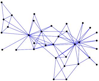
(a) Original network

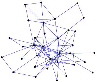
(b) Generated network

Figure 1: The Guided Graph Generator applied to a small network, the karate club network as published by Zachary (1977): (a) actual network, (b) network generated by the proposed algorithm. Both networks are drawn using the algorithm of Fruchterman and Reingold (1991).

4.1 Precision

In the first experiment, we ask to what precision the algorithms are able to generate graphs. We verify both the precision in terms of the six subgraph count statistics optimized by the proposed algorithm as shown in Table 1, as well as in terms of other common graph statistics as given in Table 3. While we expect the proposed algorithm to be precise in terms of the optimized statistics, there is a priori no reason to believe it should perform well for the other statistics. Table 5 shows the statistics of the graphs generated with this and the other algorithms for the example of the Pretty Good Privacy network as published by Boguñá et al. (2004). To measure the precision of the algorithm over all 36 investigated networks, we compute the average relative error of the proposed and other algorithms over all of them. Defining the average relative error of an algorithm with respect to a given statistic $S$ as the average of the relative errors $E^{S}$ from Equation (1) computed over all considered networks, Figure 2 shows the average relative error for all algorithms.

Table 3: Additional network statistics that are not explicitly optimized by the Guided Graph Generator algorithm, but used in our evaluation. When not noted otherwise, the definitions of the statistics we use are those given in the Handbook of the KONECT project (Kunegis, 2018). We also give network analysis methods in which these statistics are used.

Statistic	Definition	Analysis methods
$G$	Gini coefficient (Kunegis & Preusse, 2012)	Equality of the degree distribution
$\gamma$	Power law exponent (Newman, 2006, Eq. 5)	Scale-free network analysis
$c$	Clustering coefficient ($=3t/s$) (Newman et al., 2002)	Small-world analysis
$\rho$	Assortativity, i.e. Pearson correlation coefficient between the degree of connected nodes (Newman, 2003a)	Homophily analysis
$\|\mathbf{A}\|_{2}$	Spectral norm, i.e. largest absolute eigenvalue of the adjacency matrix $\mathbf{A}$	Network growth analysis
$a$	Algebraic connectivity, i.e. smallest nonzero eigenvalue of the Laplacian matrix (Fiedler, 1973)	Connectivity analysis
$\delta$	Graph diameter (Newman, 2003b)	Small-world analysis, connectivity analysis
$\delta_{\mathrm{m}}$	Average distance between two nodes (Newman, 2003b)	Small-world analysis, connectivity analysis

From the case of the Pretty Good Privacy network, and from the results over all networks, we make the following observations. The Guided Graph Generator reproduces most statistics with higher precision than the other algorithms, even statistics that are not optimized by it. The exception is the algebraic connectivity, which is not well reproduced by any algorithm, but still better reproduced by the dK model, and the diameter, which is better reproduced by the Kronecker model. We note that the average distance however is better reproduced by the Guided Graph Generator. In particular, the proposed algorithm generates graphs with better fitting values of the number of triangles $t$ and squares $q$, which are important for clustering and bipartivity characteristics. Also, the fact that the errors in the different statistics are so low for the Guided Graph Generator is an indication that the algorithm does not get stuck in any local optimum, i.e., it actually reaches an optimum very near to the requested values – the small derivation from the requested values can then be explained by combinatorial arguments.

While for individual statistics individual algorithms are as good as ours, this is not true for all statistics combined, including the non-optimized ones. The overall performance is better for more statistics with the proposed algorithm. In particular, we make the following observations:

The number of edges $m$ is matched by all algorithms, except the Kronecker model, which produces exact values only in powers of the base matrix size.

The number of wedges $s$, as an indicator of the inequality of the degree distribution, is matched approximately by all except the Erdős–Rényi, Watts–Strogatz and Barabási–Albert models. For the latter one, this is unexpected, as that algorithm is intended to produce realistic degree distributions, but can be explained by the lack of methods to adjust the algorithm to a given number of wedges. The number of claws $z$ and crosses $x$ follow similar patterns as the number of wedges.

The number of triangles $t$ is badly reproduced by most algorithms. The three classical algorithms of Erdős and Rényi, Watts and Strogatz, and Barabási and Albert without consideration of clustering produce graphs with orders of magnitudes too few triangles. The other algorithms, which do consider clustering, produce numbers of triangles within a factor of two of the correct value. All algorithms expect BTER, the algorithms of Bansal et al., Pfeiffer et al., and the Guided Graph Generator produce graphs with too few triangles. The clustering coefficient $c$ shows similar behavior.

The number of squares $q$ is matched well only by the Guided Graph Generator. It is thus the only graph generator that takes into account bipartivity among those tested.

The Gini coefficient $G$ is matched well by all algorithms based on the degree distribution, as expected. The classical algorithms of Erdős–Rényi, Watts–Strogatz and Barabási–Albert do not match it. Other algorithms match it reasonably well, and the Guided Graph Generator matches it very well.

The power law exponent $\gamma$ does not have a large range of values in the generated graphs, and thus most algorithms match it well. A notable exception is the Barabási–Albert model, which produces values that are too high by up to 50%, consistent with the fact that the actual values of the exponent seen in real graphs are for the most part smaller than the Barabási–Albert model’s theoretical value of three.

The degree assortativity $\rho$ is only matched well by the dK model, which includes the joint degree distribution as a parameter, and thus fixes $\rho$. We note that it may be possible to achieve a much more precise value of the degree assortativity for the Guided Graph Generator if it were possible to include paths of length three as a pattern, as the number of these subgraphs is related to the sum of degrees of a node’s neighbors. The number of 3-paths could however not be used as it is too expensive to keep up to date in the algorithm.

The spectral norm $\|\mathbf{A}\|_{2}$ is matched well by most algorithms, with the notable exception of the Kronecker model. This is somewhat surprising as the Kronecker model is defined using matrix multiplication.

The algebraic connectivity $a$ is badly matched by all algorithms. As the algebraic connectivity characterizes the graph globally, we should expect models that generate specific structures for the graph as a whole to match it. This is the case for the Kronecker model, even though its resulting algebraic connectivity does not match that of the input graphs.

The average distance $\delta_{\mathrm{m}}$ is matched reasonably well by all algorithms. In particular, even the Erdős–Rényi model matches it. Most algorithms produce too small diameters $\delta$ however, except for the Kronecker model.

We conclude from these observations that a precise matching of a graph’s features is complex: Even algorithms designed to reproduce a certain feature often fall only very approximately near the correct value. This is due to various reasons. For the Kronecker algorithm, this is due to the fact that only graphs whose size is a power of the initial matrix can be generated, and thus a downsampling step would be needed afterwards, complicating matters. Other methods fail because of too hard constraints – the algorithm of Bansal et al. for instance fails to generate graphs with the required amount of triangles, even though it is designed to do so, because preserving the exact degree distribution is too strong a constraint. We also observe the pattern that algorithms intended to reproduce one feature exactly often fail greatly at reproducing other features, to the point where a simpler algorithm would be better. For instance, the Watts–Strogatz model was specially constructed to produce realistic diameters and clustering, but produces unrealistic degree distributions.

Table 4: The 36 datasets used in our experiments. The names correspond to the names used by the KONECT project (Kunegis, 2018) given on konect.cc.

ucidata-gama ucidata-zachary mit adjnoun_adjacency sociopatterns-hypertext foodweb-baydry foodweb-baywet radoslaw_email contact sociopatterns-infectious arenas-meta arenas-email subelj_euroroad opsahl-usairport opsahl-ucsocial ego-facebook opsahl-openflights opsahl-powergrid subelj_jung-j subelj_jdk as20000102 advogato elec lasagne-frenchbook arenas-pgp dblp-cite lasagne-spanishbook cfinder_google ca-AstroPh eat subelj_cora ego-twitter ego-gplus as-caida20071105 hep-th-citations munmun_digg_reply

Table 5: Statistics of graphs generated to be similar to the Pretty Good Privacy network by Boguñá et al. (2004) with $n=10{,}680$. $G_{0}$ denotes the properties of the actual graph. See Tables 1, 2, and 3 for the list of graph generators as well as network statistics.

$\boldsymbol{m}$ $\boldsymbol{s}$ $\boldsymbol{z}$ $\boldsymbol{x}$ $\boldsymbol{t}$ $\boldsymbol{q}$ $\boldsymbol{G}$ $\boldsymbol{\gamma}$ $\boldsymbol{c}$ $\boldsymbol{\rho}$ $\boldsymbol{||A||_{2}}$ $\boldsymbol{a}$ $\boldsymbol{\delta}$ $\boldsymbol{\delta_{m}}$ $G_{0}$ $24{,}316$ $434{,}797$ $7{,}501{,}208$ $180{,}494{,}388$ $54{,}788$ $1{,}010{,}957$ $59\%$ $2.11$ $37.8\%$ $0.238$ $42.4$ $0.011$ $24$ $7.48$ ER $24{,}334$ $110{,}717$ $167{,}083$ $186{,}911$ $13$ $51$ $25\%$ $1.71$ $0.0\%$ $0.005$ $5.77$ $0.218$ $12$ $6.27$ MR $24{,}316$ $434{,}797$ $7{,}501{,}208$ $180{,}494{,}388$ $880$ $11{,}541$ $59\%$ $2.11$ $0.6\%$ $-0.017$ $20.2$ $0.066$ $12$ $4.70$ CL $24{,}316$ $465{,}769$ $8{,}376{,}222$ $212{,}662{,}941$ $1{,}115$ $15{,}287$ $57\%$ $1.88$ $0.7\%$ $-0.009$ $21.5$ $0.115$ $12$ $4.41$ BB $24{,}316$ $434{,}797$ $7{,}501{,}208$ $180{,}494{,}388$ $875$ $10{,}969$ $59\%$ $2.11$ $0.6\%$ $-0.021$ $20.1$ $0.067$ $13$ $4.69$ PP $24{,}316$ $517{,}195$ $9{,}275{,}916$ $232{,}859{,}495$ $6{,}795$ $28{,}076$ $57\%$ $1.75$ $3.9\%$ $-0.017$ $23.3$ $0.104$ $11$ $4.14$ BT $24{,}160$ $419{,}760$ $6{,}401{,}963$ $131{,}265{,}941$ $48{,}281$ $768{,}150$ $56\%$ $1.89$ $34.5\%$ $0.316$ $39.6$ $0.025$ $17$ $5.39$ WS $21{,}360$ $73{,}999$ $73{,}727$ $47{,}782$ $4{,}234$ $3{,}054$ $19\%$ $1.76$ $17.2\%$ $0.050$ $4.74$ $0.076$ $18$ $8.40$ BA $24{,}264$ $113{,}844$ $198{,}710$ $296{,}103$ $59$ $173$ $27\%$ $2.42$ $0.2\%$ $0.165$ $7.39$ $0.525$ $10$ $6.25$ KR $12{,}422$ $107{,}857$ $895{,}235$ $9{,}793{,}414$ $83$ $470$ $49\%$ $2.16$ $0.2\%$ $-0.056$ $11.0$ $0.067$ $15$ $5.49$ DK $23{,}206$ $420{,}091$ $7{,}214{,}212$ $172{,}216{,}188$ $6{,}306$ $138{,}845$ $60\%$ $2.10$ $4.5\%$ $0.232$ $33.8$ $0.024$ $19$ $5.37$ GG $24{,}317$ $434{,}799$ $7{,}501{,}218$ $180{,}494{,}690$ $54{,}788$ $1{,}010{,}955$ $60\%$ $2.06$ $37.8\%$ $0.032$ $33.4$ $0.003$ $28$ $8.83$

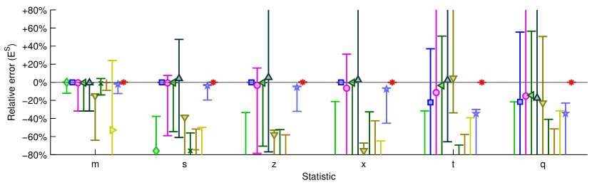
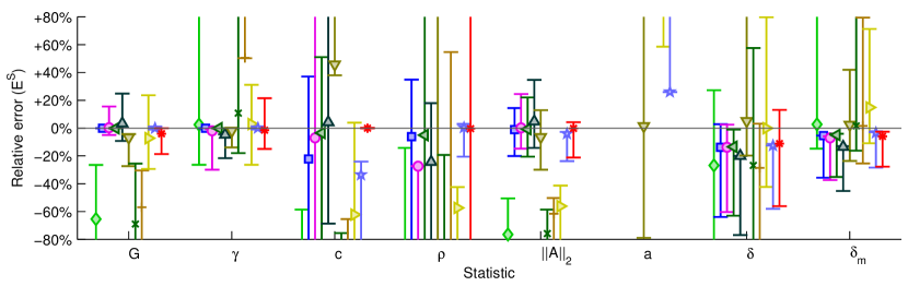
	Erdős–Rényi		Molloy–Reed		Chung–Lu		Bansal et al.
	Pfeiffer et al.		BTER		Watts–Strogatz		Barabási–Albert
	Kronecker ($k=3$)		dK ($k=2$)		Guided Graph Generator

Figure 2: Average relative error $E^{S}$ of each algorithm for each statistic $S$. The plots show the median relative error, as well as the 10^th and 90^th percentiles computed over the 36 networks in our experiments. The top row shows the statistics that are optimized by the Guided Graph Generator; the bottom row shows other statistics. The legend for the individual graph statistics is given in Tables 1 and 3.

4.2 Scalability of the Guided Graph Generator

We have shown in Section 3.3 that each iteration step of the Guided Graph Generator has a runtime of $O(m)$, where $m$ is the number of edges in the graph. The number of iterations needed for the proposed algorithm to converge cannot be deduced theoretically, but a simple heuristic dictates that if all nodes should be visited, then the number of iterations will also be linear in $n$, giving a total runtime of $O(mn)$.

For all networks that we use in this paper, the Guided Graph Generator as implemented in the Matlab programming language took at most 28 hours to complete, and used no more than 5 GiB of memory. For comparison, fitting the Kronecker model is said to take from 24 to 48 hours and 32 GiB of RAM for networks with 200,000–300,000 nodes (Sala et al., 2010). In order to measure the runtime’s exponent as a function of network size, we show in Figure 3 the runtime and network size, on a doubly logarithmic plot. The results are consistent with a runtime quadratic in network size. The same experiments with the other methods (not shown) resulted in similarly quadratic runtimes, except for the Kronecker model, whose fitting algorithm was slow with small networks, but not slower for larger networks, making it impossible to make any statement about its asymptotic runtime as a function of network size.

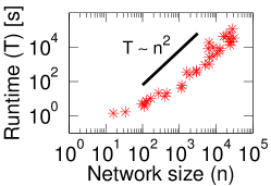
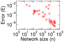
Figure 3: The error and runtime of the Guided Graph Generator in function of network size, i.e. the number $n=|V|$ of nodes.

4.3 Analysis of Characteristic Network Distributions

Network statistics do not uniquely determine a graph, and we must thus ask whether the consideration of a few network statistics is sufficient to claim that a generated network is realistic. In order to do this, we consider multiple properties of networks that are not represented by individual numbers but by a whole distribution of values: the degree distribution, the clustering coefficient distribution, the distance distribution, and the spectral distribution. All plots shown in this section are for the Pretty Good Privacy network.

Degree Distribution. The degree of a node is the number of its neighbors, and accordingly the degree distribution of a network can be considered. Real-world networks have been observed, many times, to have degree distributions with power-law tails (see e.g. Clauset et al., 2009). This is as opposed to models such as Erdős–Rényi random graphs, which have Poisson degree distributions. Figure 4 shows the degree distributions of the graphs generated by the various methods, excluding those methods that take the degree distribution as input and thus generate the exact correct degree distribution. We observe that all methods except those of Erdős–Rényi, Watts–Strogatz and Barabási–Albert produce well-fitting degree distributions. A further observation can be made about the Guided Graph Generator: Its degree distribution is not as smooth as the original one, but deviates slightly in alternate directions. We explain this by the fact that the proposed algorithm takes not the full degree distribution as input, but only the number of edges, wedges, claws and crosses, i.e. the number of $k$-stars for $k=1,2,3,4$, where we interpret an edge as a 1-star. Since the numbers of $k$-stars are related to the $k$-th moments of the degree distribution, the proposed algorithm generates graphs whose degree distributions are correct up to these modified moments. We also note the incidental similarity of graphs generated by the proposed algorithm to Kronecker graphs, as those too tend to have unbalanced degree distribution, containing rough steps.

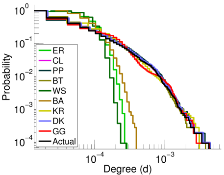
Figure 4: Comparison of the complementary cumulative degree distributions generated by the different models for the Pretty Good Privacy network.

Clustering Coefficient Distribution. The clustering coefficient $c$ as defined previously is a global characteristic, denoting the probability that two nodes with a common neighbor are connected. This measure of clustering can also be applied to individual nodes, giving the local clustering coefficient, i.e. the probability that two neighbors of a given node are connected. The distribution of the local clustering coefficient over all nodes then gives a network’s clustering coefficient distribution. Figure 5 shows the clustering coefficient distribution of the networks generated by each algorithm. We observe that the clustering coefficient distributions of the different graph models vary wildly: Models that do not take into account clustering have, as expected, almost only nodes with a local clustering coefficient near zero. The algorithm of Bansal et al., as well as that of Pfeiffer et al. produce slightly more correct clustering coefficient distributions. Finally, the best clustering coefficient distribution are generated by BTER and by the Guided Graph Generator. For BTER, this is to be excepted, as BTER takes the local clustering coefficient distribution as input.

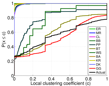
Figure 5: Comparison of the local clustering coefficient distributions generated by the different models for the Pretty Good Privacy network.

Distance Distribution. The distance between two nodes of a graph is defined as the minimum number of edges needed to reach one node from the other. Distances determine the dynamics of communication within a network, and are therefore of importance for many types of networks. The distance distribution is the distribution of distance values over all node pairs. Thus, the distance distribution extends the average path length $\delta_{\mathrm{m}}$ and the maximal path length $\delta$ (the diameter) to give information about the distribution over all path lengths. In order to plot the distance distribution, we use its cumulative distribution function $H(d)$, i.e., the proportion of all node pairs that are reachable in at most $d$ edges. The resulting plots in Figure 6 show this function $H(d)$ on an inverse logistic scale, i.e. we show $\Phi^{-1}(H(d))=\ln(H(d)/(1-H(d)))$ on the Y axis, where $\Phi(x)=1/(1+e^{-x})$ is the logistic function. The reason for choosing a logistic scale is to give particular attention to the tails of the distribution, as those are otherwise not captured by the average path length. We choose the cumulative distribution for visualization as it is related to the Kolmogorov–Smirnov test (and thus the Kolmogorov–Smirnov distance) which measures the similarity of two distributions. As none of the tested algorithms optimizes directly for distances in the graphs, none produces a particularly well matching distance distribution. The Guided Graph Generator, too, does not produce a distance distribution that matches the given network with precision. As noted before though, we have identified that Kronecker graphs match original graphs well in their diameter, i.e. the maximum of the distance distribution, and the proposed algorithm matches original graphs well in the average of the distance distribution. It remains thus an open problem to define a graph model that reproduces the distance distribution accurately.

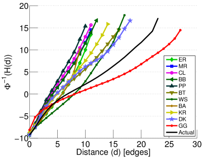
Figure 6: Comparison of the distance distributions generated by the different models for the Pretty Good Privacy network.

Spectral Distribution. An important characterization of a graph is in terms of the spectrum of its adjacency matrix, which captures information about the number of cycles of different lengths it contains. We consider the distribution of the eigenvalues of a graph’s normalized adjacency matrix $\mathbf{N}$. This matrix is an $n\times n$ matrix, defined by $\mathbf{N}_{uv}=1/\sqrt{\mathbf{d}_{u}\mathbf{d}_{v}}$ when $u$ and $v$ are connected, and $\mathbf{N}_{uv}=0$ otherwise. $\mathbf{N}$ is symmetric, and its real eigenvalues lie in the interval $[-1,+1]$. The set of eigenvalues of the matrix $\mathbf{N}$ encodes information about the number of cycles of length $k$ for all $k\geq 0$, in that the $k$-th moment of the eigenvalues equals the probability of a random walk of length $k$ to return to its starting point. Thus, the spectral distribution is an extension of the number of triangles $t$ and squares $q$ to longer cycles, and comparing the spectrum of $\mathbf{N}$ serves as a test of the accuracy for graph generators to generate graphs in which the number of higher-order cycles is realistic.

Figure 7 shows the spectral distribution of the networks generated by the different methods. We observe that none of the algorithms reproduces the spectral distribution precisely. The methods that come the closest are BTER and dK. A few observations can be made from the specific spectra of individual models: The Kronecker model, as well as the model of Pfeiffer et al. have a large number of near-zero eigenvalues; this indicates that they produce graphs with many unconnected or badly-connected vertices. The Guided Graph Generator algorithm produces a graph with many eigenvalues equal to one, indicating that it creates too many small non-empty clusters unconnected to the rest of the network. Both of these are errors in the reconstruction, as the original graph does not have these properties.

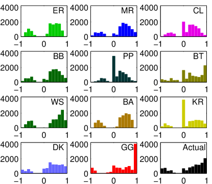
Figure 7: Comparison of the normalized spectral distributions generated by the different models for the Pretty Good Privacy network, based on the eigenvalues of the normalized adjacency matrix $\mathbf{N}$ of the networks.

4.4 Convergence of the Guided Graph Generator

The proposed Guided Graph Generator algorithm is greedy-like in that it performs only local optimizations by adding and removing individual edges. Thus, there is no theoretical guarantee that the algorithm cannot get stuck in a local optimum. As an empirical test of the behavior of the algorithm in real-world cases, we may inspect Figure 3: The error $E$ as a function of the network size $n$ is decreasing, indicating that the generated graphs are reasonably close to the requested target values, and that the relative error is smaller for larger graphs. Thus, while it would be conceivable that the algorithm gets stuck in a local optimum for certain ranges of input subgraph counts, this appears to not be the case. We can conclude from this that the property of a graph that makes the Guided Graph Generator get stuck is a very rare property in real-world graphs.

As to the convergence speed of the Guided Graph Generator, we may interrupt the algorithm at any timepoint to get a generated graph that is not optimal in terms of our stopping criteria, but is faster to compute. Although the algorithm reduces the error $E$ over time, it is a priori not clear whether the algorithm converges at all, and how changes for each individual statistic contribute to the error. Thus, we show in Figure 8 the overall error $E$ (top plot) and the relative error $E^{S}$ for each statistic $S$ (lower plot) for the Pretty Good Privacy network. We observe phases in which each statistic is optimized, while in some phases some statistics do not improve, and sometimes even regress. In fact, the number of edges, which is initially correct due to the algorithm starting with an Erdős–Rényi network, increases at first to allow the other count statistics to be corrected. Once the other statistics approach their intended values, the number of edges decreases back to its correct value. The three $k$-star counts (wedges, claws and crosses) increase fast at first, and also surpass their target values only to come back later, allowing the triangle and square count to be adjusted over time. We note that the number of $k$-stars increases faster for higher $k$, which we explain by the fact that adding edges to a high-degree node makes them grow faster, which indicates that in a first phase, the degree distribution is adjusted by the algorithm, while the clustering statistics (the number of triangles and squares), reach their intended values much more slowly in a second phase. Figure 8 also shows the influence of the parameter $\epsilon$ on the runtime of the proposed algorithm, as the number of steps $i$ is linear in the runtime of the algorithm. The experiment shows that the algorithm has runtime sublinear in $\epsilon^{-1}$.

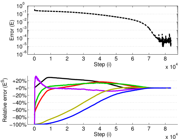
Figure 8: Convergence of the Guided Graph Generator for the Pretty Good Privacy network by Boguñá et al. (2004). Upper plot: evolution of the error $E$. Lower plot: Evolution of the individual relative errors $E^{S}$.

In terms of convergence speed, we may also compare the Guided Graph Generator to other algorithms directly in two ways: (1) Does our algorithm generate a better graph when given a runtime equal to that of another algorithm? (2) Is our algorithm faster than other algorithms when generating graphs of equal quality? Both questions can be answered by inspecting the error $E$ in function of runtime of the proposed algorithm, and comparing it to the runtime and error of other algorithms. This experiment is shown for the Pretty Good Privacy network in Figure 9. First of all, we can observe that the Guided Graph Generator is slower and more precise than the other tested algorithms. This is true not only for the one shown network, but for all 36 networks that we tested. Comparing other algorithms with ours at their runtime, or at their precision shows that only BTER and the dK model are consistently faster at equal precision and more precise at the same runtime. Note however that these models use a $O(n)$- and $O(n^{2})$-dimensional parameter space.

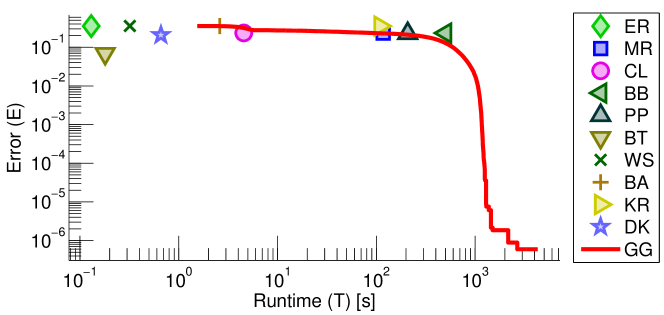
Figure 9: The error $E$ in function of runtime for the Pretty Good Privacy network. The proposed Guided Graph Generator is shown as a curve, reflecting the error of the current solution at different timepoints. Other algorithms are shown as points. Note that the Guided Graph Generator has by far the smallest error out of all algorithms; it is however not the fastest.

5 Limitations of the Approach

Beyond the numerical results presented in the preceding section, we address here several important issues related to the proposed Guided Graph Generator algorithm and to graph generators based on network statistics in general.

5.1 Precision vs Underlying Models

A common criterion for evaluating graph generators is the motivation for the specific underlying graph generation rules. For instance, the Barabási–Albert model is very well justified by the principle of preferential attachment, which is (at least conceptually) a phenomenon believed to exist in the growth of real networks, and thus gives it a justification: Even if the Barabási–Albert model does not produce the most realistic graphs (our experiments show that several other algorithms beat it at that task), it nevertheless allows one to understand why real-world networks have the properties that they have by proposing a mechanism that leads to them. This is specifically not the case for the Guided Graph Generator, which takes the properties of an existing graph as input and reproduces these in a synthetic graph. In fact, we must stress that the iteration steps performed by the algorithm do not correspond to an actual graph evolution phenomenon, but purely to an optimization procedure. Therefore, we come to the conclusion that the algorithm is not a graph model, but instead a graph generator, a task at which it outperforms other algorithms.

5.2 Comparison of Statistics

The Guided Graph Generator proposed in this paper indeed generates synthetic graphs with a high precision – both in terms of the properties it optimizes, as well as for other properties such as the average distance, the assortativity and the spectral norm. The properties that it does not reproduce well are those for which no algorithm yet exists that reproduces them: the algebraic connectivity $a$, the spectral distribution of the normalized adjacency matrix $\mathbf{N}$, and the distance distribution. However, the proposed algorithm does not perform as well as Kronecker graphs in terms of the diameter. Also, specific other algorithms that optimize for specific properties are better at reproducing these properties: the degree distribution for the algorithms of Molloy–Reed and Bansal et al., the clustering coefficient for BTER, and the assortativity for the dK model.

In our experiments, we also made notable observations on existing network models. For instance both the Kronecker and the dK models produce very unrealistic clustering coefficient distributions, even though at least the Kronecker model includes clustering by way of its base matrix.

5.3 Precision vs Speed

In terms of precision vs speed the Guided Graph Generator is very clearly placed on the precision side. In fact, even algorithms known to be slow such as Kronecker fitting are faster than the proposed algorithm in many cases. We note that the algorithm could be made faster simply by reimplementing it in C or C++; we did not do this as our main concern was precision – the fact that runtime was comparable between algorithms is enough to make the algorithm tractable for many practical applications. Another avenue for improving the runtime of the algorithm is by parallelization. First, the inner loop of the algorithm over all statistics $S\in\mathcal{S}$ can be executed in parallel and second, each updating step uses only local information, and thus also lends itself to parallelization.

5.4 Conflicting or Impossible Inputs

In our examples and experiments, we have taken the subgraph counts used as input to the Guided Graph Generator from actual given real-world graphs. In fact, Algorithm 1 as described in this paper takes an input graph $G_{0}$ from which subgraph counts are taken. This makes sure that the target subgraph counts optimized by the algorithm are realizable. However, nothing prevents us from using numbers as input which are not realizable. For instance, constructing a simple graph with 10 edges and 50 triangles is an impossible task – a graph with 10 edges can have at most 10 triangles; this is realized by the complete graph on five nodes. Faced with such inputs, the Guided Graph Generator generates graphs that are degenerate: They don’t come near the requested subgraph count values, but instead are extremal, i.e., they often contain large cliques, which are the most efficient way to create a large number of certain subgraphs. This can lead to certain interesting subcases: When a very large number of squares is requested at the same time than a very small number of triangles, the algorithm converges to a complete bipartite graph (i.e., a biclique). Note however that in general, it is very difficult to determine whether a given combination of subgraph count is realizable. As an example, the general problem to determine whether there exists a graph with a given number of nodes, edges and triangles does not have a more efficient known solution that enumerating all graphs with the requested properties.

5.5 Statistical Properties of the Guided Graph Generator

For graph generation algorithms, it is a useful property to derive the distribution of statistical values of the generated graphs when the algorithm is run multiple times, or when the algorithm is used as a sampling algorithm, i.e., subsequent graphs it generates are used as output. The proposed algorithm however does not try to generate a set of graphs whose properties follow given distributions, but instead is meant to find a single graph whose properties are as near as possible to given target values. As a result, the distribution of graph statistics, if the algorithm were to be run for a large number of iterations, would not converge towards any meaningful distribution, and thus cannot be characterized as a Markov chain. In fact, due to the greedy-like nature of the algorithm, the distribution of statistics of generated graphs would be distributed (in a most likely non-normal way) around the target values. Thus, the Guided Graph Generator cannot be used to sample multiple graphs with a given distribution of statistics, but instead can only be used to find a graph whose properties are as near as possible to the target values. Note that an algorithm that generates a series of graphs with a predictable distribution of properties will necessarily produce graphs with a larger average error than an algorithm that outputs only a single graph with minimal error, but cannot be used for sampling. The distribution of graph statistics which are not optimized explicitly by the proposed algorithm thus cannot be derived, and thus the experiments of Figure 2 (bottom) are needed to ascertain that the non-optimized statistics, too, have realistic values.

A further note can be made to compare the Guided Graph Generator with approaches that use Gibbs sampling to generate graphs from an exponential random graph model. Characterizing the distribution of statistics generated by a given iterative graph model is possible in principle. For instance, exponential random graph models (ERGMs) can be generated by Gibbs sampling. In an ERGM, the probability of each individual graph $G$ is proportional to $\exp\{a_{1}x_{1}(G)+a_{2}x_{2}(G)+\ldots\}$, where the $x_{i}(G)$ are the used graphs statistics, and the values $\{a_{i}\}$ are the parameters of the model. Thus, Gibbs sampling can be implemented by asking, at each step of the iteration, whether an edge should be flipped, and basing the decision on the ratio of probabilities between the graph before and after the putative flip, leading to an expression involving only the difference in the different graph statistics. While this iterative algorithm will generate graphs from the desired exponential random graph model, it does not allow to easily generate graphs that are similar to a given input graph: In order to execute this algorithm, the parameters $a_{i}$ must be known, and in order to determine these parameters, very computationally expensive Monte-Carlo Markov chain estimation is necessary, as the only relationship between the $a_{i}$ and the statistics of the target graph is that they are related by a monotonously growing function (Robins et al., 2007). Thus, the Guided Graph Generator can be understood as bypassing the issue of computing the parameter values $a_{i}$, and instead opting to use the values of the original graph’s statistics as parameters. The price for this simplification however is that it is not anymore possible to characterize the distribution of the generated graphs, but only to measure empirically that their convergence is good enough for a given practical application.

6 Conclusion

To summarize this article, we have presented an evaluation of common graph generation algorithms in terms of numerical properties of the graphs they generate, and shown that these common algorithms do not perform ideally at that task, leading us to propose a novel algorithm for it. The proposed algorithm, the Guided Graph Generator, was shown to beat previous algorithms at the task of generating networks with specific values of network statistics, with the exception of graph properties that are specifically optimized for by specific algorithms. In particular, the proposed algorithm is able to generate graphs with a given number of squares, and thus with a given bipartivity measure, better than all other tested graph generators. On the other hand, we were not able to beat Leskovec et al.’s Kronecker model in terms of the generated graph’s diameter. Despite these positive results, the proposed algorithm is only a pure graph generator, and must be carefully distinguished from the related but distinct concept of graph models: By construction, the proposed algorithm does not explain why real-world networks have the properties that they have.

In principle, the Guided Graph Generator algorithm as described in Algorithm 1 can be applied to any numerical graph statistic, making it possible to also optimize directly for instance for the algebraic connectivity, diameter or assortativity. In practice, doing so is highly expensive, as new values of the statistics must be computed for each node at each step. In experiments, we were barely able to generate such graphs based on the smallest network in our collection, the Zachary karate club graph with 34 nodes. Thus, this variant is prohibited as long as no fast updating algorithms are available for these statistics. The same is true to a lesser extent for other count statistics: While the expressions for the update of the number of crosses and squares is tractable, higher star, cycle and clique counts require much more complex expressions. In particular, the ability to compute the count of 3-paths in an efficient way may make it possible to generate graphs with more accurate values of the degree assortativity.

For the algebraic connectivity, the eigenvalues of the normalized adjacency matrix $\mathbf{N}$, and the distance distribution, none of the tested models reproduce realistic values, and it is an open problem to formulate a graph model that fits each of them.

Additional Information

Availability of Data and Material. The datasets used in the experiments are all part of the KONECT project. The names of the dataset used are given in Table 4. All datasets are either available for download via the KONECT project, or available on request from the authors, in case where a public distribution is not allowed.

Funding. This research was partly funded by the EPSRC (EP/P004024 and Cambridge University GCRF), and by the European Regional Development Fund (ERDF/FEDER – IDEES).

Authors’ Contributions. The method was developed by J. Kunegis, J. Sun, and E. Yoneki. The experiments were implemented and executed by J. Kunegis. The manuscript was written by J. Kunegis, J. Sun, and E. Yoneki.

Acknowledgments. We thank Valentin Dalibard and Christoph Schaefer for helpful comments on our experiments, as well as for helping with executing third-party graph generator implementations.

References

- (1)
- Albert & Barabási (2002) Albert, R. & Barabási, A.-L. (2002), ‘Statistical mechanics of complex networks’, Rev. of Mod. Phys. 74(1), 47–97.
- Ángeles Serrano & Boguñá (2005) Ángeles Serrano, M. & Boguñá, M. (2005), ‘Tuning clustering in random networks with arbitrary degree distributions’, Phys. Rev. E 72(3), 036133.
- Bansal et al. (2009) Bansal, S., Khandelwal, S. & Meyers, L. A. (2009), ‘Exploring biological network structure with clustered random networks’, BMC Bioinform. 10(1), 1–15.
- Barabási & Albert (1999) Barabási, A.-L. & Albert, R. (1999), ‘Emergence of scaling in random networks’, Science 286(5439), 509–512.
- Boguñá et al. (2004) Boguñá, M., Pastor-Satorras, R., Díaz-Guilera, A. & Arenas, A. (2004), ‘Models of social networks based on social distance attachment’, Phys. Rev. E 70(5), 056122.
- Chakrabarti & Faloutsos (2006) Chakrabarti, D. & Faloutsos, C. (2006), ‘Graph mining: Laws, generators, and algorithms’, ACM Comput. Surv. 38.
- Chatterjee et al. (2011) Chatterjee, S., Diaconis, P. & Sly, A. (2011), ‘Random graphs with a given degree sequence’, Ann. Appl. Probab. 21(4), 1400–1435.
- Chung & Lu (2002) Chung, F. & Lu, L. (2002), ‘The average distance in a random graph with given expected degrees’, Proc. Natl. Acad. Sci. U.S.A. 99(25), 15879–15882.
- Clauset et al. (2009) Clauset, A., Shalizi, C. R. & Newman, M. E. J. (2009), ‘Power-law distributions in empirical data’, SIAM Rev. 51(4), 661–703.
- Erdős & Rényi (1959) Erdős, P. & Rényi, A. (1959), ‘On random graphs I’, Publ. Math. Debrecen 6, 290–297.
- Estrada & Rodríguez-Velázquez (2005) Estrada, E. & Rodríguez-Velázquez, J. A. (2005), ‘Spectral measures of bipartivity in complex networks’, Phys. Rev. E 72(4), 046105.
- Fiedler (1973) Fiedler, M. (1973), ‘Algebraic connectivity of graphs’, Czechoslov. Math. J. 23(98), 298–305.
- Fruchterman & Reingold (1991) Fruchterman, T. M. J. & Reingold, E. M. (1991), ‘Graph drawing by force-directed placement’, Software: Pract. and Exp. 21(11), 1129–1164.
- Gleich & Owen (2012) Gleich, D. & Owen, A. (2012), ‘Moment-based estimation of stochastic Kronecker graph parameters’, Internet Math. 8(3), 232–256.
- Goodreau (2007) Goodreau, S. M. (2007), ‘Advances on exponential random graph (p*) models applied to a large social network’, Soc. Netw. 29(2), 231–248.
- Gutfraind et al. (2015) Gutfraind, A., Safro, I. & Meyers, L. A. (2015), Multiscale network generation, in ‘Proc. Int. Conf. on Inf. Fusion’, pp. 158–165.
- Janson (1988) Janson, S. (1988), ‘Normal convergence by higher semi-invariants with applications to sums of dependent random variables and random graphs’, Ann. Probab. 16(1), 305–312.
- KronFit (2017) KronFit (2017), https://github.com/snap-stanford/snap. Accessed: 2017-04-20.
- Kunegis (2013) Kunegis, J. (2013), KONECT – The Koblenz Network Collection, in ‘Proc. Int. Conf. on World Wide Web Companion’, pp. 1343–1350.
- Kunegis (2018) Kunegis, J. (2018), ‘Handbook of network analysis [KONECT project]’, CoRR abs/1402.5500(v4).
- Kunegis & Preusse (2012) Kunegis, J. & Preusse, J. (2012), Fairness on the web: Alternatives to the power law, in ‘Proc. Web Sci. Conf.’, pp. 175–184.
- Leskovec et al. (2010) Leskovec, J., Chakrabarti, D., Kleinberg, J., Faloutsos, C. & Ghahramani, Z. (2010), ‘Kronecker graphs: An approach to modeling networks’, J. Mach. Learn. Res. 11, 985–1042.
- Mahadevan et al. (2007) Mahadevan, P., Hubble, C., Krioukov, D., Huffaker, B. & Vahdat, A. (2007), ‘Orbis: Rescaling degree correlations to generate annotated Internet topologies’, SIGCOMM Comput. Commun. Rev. 37(4), 325–336.
- Miller (2009) Miller, J. C. (2009), ‘Percolation and epidemics in random clustered networks’, Phys. Rev. E 80, 020901.
- Molloy & Reed (1995) Molloy, M. & Reed, B. (1995), ‘A critical point for random graphs with a given degree sequence’, Random Struct. Algorithms 6(2/3), 161–179.
- Motalleb et al. (2013) Motalleb, S., Aliakbary, S. & Habibi, J. (2013), ‘GMSCN: Generative model selection using a scalable and size-independent complex network classifier’, Chaos: An Interdiscip. J. of Nonlinear Sci. 23(4), 043127.
- Newman (2003a) Newman, M. E. J. (2003a), ‘Mixing patterns in networks’, Phys. Rev. E 67, 026126.
- Newman (2003b) Newman, M. E. J. (2003b), ‘The structure and function of complex networks’, SIAM Rev. 45(2), 167–256.
- Newman (2006) Newman, M. E. J. (2006), ‘Power laws, Pareto distributions and Zipf’s law’, Contemp. Phys. 46(5), 323–351.
- Newman (2009) Newman, M. E. J. (2009), ‘Random graphs with clustering’, Phys. Rev. Lett. 103, 058701.
- Newman et al. (2002) Newman, M. E. J., Watts, D. J. & Strogatz, S. H. (2002), ‘Random graph models of social networks’, Proc. Natl. Acad. Sci. U.S.A. 99, 2566–2572.
- OEIS (2017) OEIS (2017), ‘A006785 – number of triangle-free graphs on vertices – The On-Line Encyclopedia of Integer Sequences’.
- Olbrich et al. (2010) Olbrich, E., Kahle, T., Bertschinger, N., Ay, N. & Jost, J. (2010), ‘Quantifying structure in networks’, Eur. Phys. J. B 77, 239.
- Pfeiffer et al. (2012) Pfeiffer, J. J., La Fond, T., Moreno, S. & Neville, J. (2012), Fast generation of large scale social networks with clustering, in ‘Proc. Int. Conf. on Knowl. Discov. and Data Min.’, pp. 154–165.
- Read (1981) Read, R. C. (1981), A survey of graph generation techniques, in K. L. McAvaney, ed., ‘Comb. Math. VIII’, Vol. 884 of Lecture Notes in Math., Springer, pp. 77–89.
- Ritchie et al. (2016) Ritchie, M., Berthouze, L. & Kiss, I. Z. (2016), ‘Generation and analysis of networks with a prescribed degree sequence and subgraph family: Higher-order structure matters’, J. of Complex Netw. 5(1), 1–31.
- Robins et al. (2007) Robins, G., Snijders, T., Wang, P., Handcock, M. & Pattison, P. (2007), ‘Recent developments in exponential random graph (p*) models for social networks’, Soc. Netw. 29, 192–215.
- Ruciński (1988) Ruciński, A. (1988), ‘When are small subgraphs of a random graph normally distributed?’, Prob. Th. Rel. Fields 78, 1–10.
- Sala et al. (2010) Sala, A., Cao, L., Wilson, C., Zablit, R., Zheng, H. & Zhao, B. Y. (2010), Measurement-calibrated graph models for social network experiments, in ‘Proc. Int. World Wide Web Conf.’, pp. 861–870.
- Seshadhri et al. (2012) Seshadhri, C., Kolda, T. G. & Pinar, A. (2012), ‘Community structure and scale-free collections of Erdős–Rényi graphs’, Phys. Rev. E 85(5), 056109.
- Snijders et al. (2006) Snijders, T. A. B., Pattison, P. E. & Handcock, M. S. (2006), ‘New specifications for exponential random graph models’, Sociol. Methodol. 36(1), 99–153.
- Tabourier et al. (2011) Tabourier, L., Roth, C. & Cointet, J.-P. (2011), ‘Generating constrained random graphs using multiple edge switches’, J. Exp. Algorithmics 16, 1.7:1.1–1.7:1.15.
- Watts & Strogatz (1998) Watts, D. J. & Strogatz, S. H. (1998), ‘Collective dynamics of ‘small-world’ networks’, Nature 393(1), 440–442.
- Waxman (1988) Waxman, B. M. (1988), ‘Routing of multipoint connections’, J. on Sel. Areas in Commun. 6(9), 1617–1622.
- White & Wilson (2007) White, D. & Wilson, R. C. (2007), Spectral generative models for graphs, in ‘Proc. Int. Conf. Image Anal. and Process.’, pp. 35–42.
- Xiao & Hancock (2006) Xiao, B. & Hancock, E. R. (2006), A spectral generative model for graph structure, in ‘Proc. Jt. IAPR Int. Workshops on Stat. Tech. in Pattern Recognit. and Struct. and Syntactic Pattern Recognit.’, pp. 173–181.
- Ying & Wu (2009) Ying, X. & Wu, X. (2009), Graph generation with prescribed feature constraints, in ‘Proc. SIAM Int. Conf. on Data Min.’, pp. 966–977.
- Zachary (1977) Zachary, W. (1977), ‘An information flow model for conflict and fission in small groups’, J. of Anthropol. Res. 33, 452–473.