An Information-Theoretic Perspective on
Variance-Invariance-Covariance Regularization

Abstract

In this paper, we provide an information-theoretic perspective on Variance-Invariance-Covariance Regularization (VICReg) for self-supervised learning. To do so, we first demonstrate how information-theoretic quantities can be obtained for deterministic networks as an alternative to the commonly used unrealistic stochastic networks assumption. Next, we relate the VICReg objective to mutual information maximization and use it to highlight the underlying assumptions of the objective. Based on this relationship, we derive a generalization bound for VICReg, providing generalization guarantees for downstream supervised learning tasks and present new self-supervised learning methods, derived from a mutual information maximization objective, that outperform existing methods in terms of performance. This work provides a new information-theoretic perspective on self-supervised learning and Variance-Invariance-Covariance Regularization in particular and guides the way for improved transfer learning via information-theoretic self-supervised learning objectives.

1 Introduction

Self-Supervised Learning (SSL) methods learn representations by optimizing a surrogate objective between inputs and self-defined signals. For example, in SimCLR (Chen et al., 2020), a contrastive loss is used to make representations for different versions of the same image similar while making representations for different images different. These pre-trained representations are then used as a feature extractor for downstream supervised tasks such as image classification, object detection, and transfer learning (Caron et al., 2021; Chen et al., 2020; Misra and Maaten, 2020; Shwartz-Ziv et al., 2022). Despite their success in practice, only a few works (Arora et al., 2019; Lee et al., 2021a) have sought to provide theoretical insights about the effectiveness of SSL.

Recently, information-theoretic methods have played a key role in several advances in deep learning—from practical applications in representation learning (Alemi et al., 2016) to theoretical investigations (Xu and Raginsky, 2017; Steinke and Zakynthinou, 2020; Shwartz-Ziv, 2022). Some works have attempted to use information theory for SSL, such as the InfoMax principle (Linsker, 1988) in SSL (Bachman et al., 2019). However, these works often present objective functions without rigorous justification, make implicit assumptions (Kahana and Hoshen, 2022; Wang et al., 2022; Lee et al., 2021b), and explicitly assume that the deep neural network mappings are stochastic—which is rarely the case for modern neural networks. See Shwartz-Ziv and LeCun (2023) for a detailed review.

This paper presents an information-theoretic perspective on Variance-Invariance-Covariance Regularization (VICReg). We show that the VICReg objective is closely related to approximate mutual information maximization, derive a generalization bound for VICReg, and relate the generalization bound to information maximization. We show that under a series of assumptions about the data, which we validate empirically, our results apply to deterministic deep neural network training and do not require further stochasticity assumptions about the network. To summarize, our key contributions are as follows:

1. We shift the stochasticity assumption to the deep neural network inputs to study deterministic deep neural networks from an information-theoretic perspective.

2. We relate the VICReg objective to information-theoretic quantities and use this relationship to highlight the underlying assumptions of the objective.

3. We study the relationship between the optimization of information-theoretic quantities and predictive performance in downstream tasks by introducing a generalization bound that connects VICReg, information theory, and downstream generalization.

4. We present information-theoretic SSL methods based on our analysis and empirically validate their performance.

2 Background & Preliminaries

We first introduce the technical background for our analysis.

Continuous Piecewise Affine (CPA) Mappings.

A rich class of functions emerges from piecewise polynomials: spline operators. In short, given a partition $\Omega$ of a domain $\mathbb{R}^{D}$, a spline of order $k$ is a mapping defined by a polynomial of order $k$ on each region $\omega\in\Omega$ with continuity constraints on the entire domain for the derivatives of order $0$,…,$k-1$. As we will focus on affine splines ($k=1$), we define this case only for concreteness. A $K$-dimensional affine spline $f$ produces its output via

$$f(\bm{z})=\sum\nolimits_{\omega\in\Omega}(\bm{A}_{\omega}\bm{z}+\bm{b}_{\omega})\mathbbm{1}_{\{\bm{z}\in\omega\}},$$ (1)

with input $\bm{z}\in\mathbb{R}^{D}$ and $\bm{A}_{\omega}\in\mathbb{R}^{K\times D},\bm{b}_{\omega}\in\mathbb{R}^{K},\forall\omega\in\Omega$ the per-region slope and offset parameters respectively, with the key constraint that the entire mapping is continuous over the domain $f\in\mathcal{C}^{0}(\mathbb{R}^{D})$. Spline operators and especially affine spline operators have been widely used in function approximation theory (Cheney and Light, 2009), optimal control (Egerstedt and Martin, 2009), statistics (Fantuzzi et al., 2002), and related fields.

Deep Neural Networks as CPA Mappings.

A deep neural network (DNN) is a (non-linear) operator $f_{\Theta}$ with parameters $\Theta$ that map a input $\bm{x}\in\mathbb{R}^{D}$ to a prediction $\bm{y}\in\mathbb{R}^{K}$. The precise definitions of DNN operators can be found in Goodfellow et al. (2016). To avoid cluttering notation, we will omit $\Theta$ unless needed for clarity. The only assumption we require for our analysis is that the non-linearities present in the DNN are CPA mappings—as is the case with (leaky-) ReLU, absolute value, and max-pooling operators. The entire input–output mapping then becomes a CPA spline with an implicit partition $\Omega$, the function of the weights and architecture of the network (Montufar et al., 2014; Balestriero and Baraniuk, 2018). For smooth nonlinearities, our results hold using a first-order Taylor approximation argument.

Self-Supervised Learning.

Joint embedding methods learn DNN parameters $\Theta$ without supervision and input reconstruction. The difficulty of self-supervised learning (SSL) is generating a good representation for downstream tasks whose labels are unavailable during self-supervised training while avoiding trivial solutions where the model maps all inputs to constant output. Many methods have been proposed to solve this problem (see Balestriero and LeCun (2022) for a summary and connections between methods). Contrastive methods, such as SimCLR (Chen et al., 2020) and its InfoNCE criterion (Oord et al., 2018), learn representations by contrasting positive and negative examples. In contrast, non-contrastive methods employ different regularization methods to prevent collapsing of the representation and do not explicitly rely on negative samples. Some methods use stop-gradients and extra predictors to avoid collapse (Chen and He, 2021; Grill et al., 2020) while Caron et al. (2020) use an additional clustering step. Of particular interest to us is the Variance-Invariance-Covariance Regularization method(VICReg;  Bardes et al. (2021)) that considers two embedding batches $\bm{Z}=\left[f(\bm{x}_{1}),\dots,f(\bm{x}_{N})\right]$ and $\bm{Z}^{\prime}=\left[f(\bm{x}^{\prime}_{1}),\dots,f(\bm{x}^{\prime}_{N})\right]$ each of size $(N\times K)$. Denoting by $\bm{C}$ the $(K\times K)$ covariance matrix obtained from $[\bm{Z},\bm{Z}^{\prime}]$, the VICReg triplet loss is given by

$$\SwapAboveDisplaySkip\mathcal{L}=\frac{1}{K}\sum_{k=1}^{K}(\alpha\text{Var}(Z_{k})+\beta\text{Cov}(Z_{k},Z_{k^{\prime}}))+\gamma\text{Inv}(Z_{k},Z_{k^{\prime}}),$$ (2)

where

$$\SwapAboveDisplaySkip\text{Var}(Z_{k}) =\max(0,\gamma-\sqrt{\bm{C}_{k,k}+\epsilon})\qquad~{}$$ (3)

$$\text{Cov}(Z_{k},Z_{k^{\prime}}) =\sum\nolimits_{k^{\prime}\neq k}\left(\bm{C}_{k,k^{\prime}}\right)^{2}$$ (4)

$$\text{Inv}(Z_{k},Z_{k^{\prime}}) =\|\bm{Z}_{k}-\bm{Z}_{k^{\prime}}\|_{F}^{2}/N.$$ (5)

Deep Networks and Information-Theory.

Recently, information-theoretic methods have played an essential role in advancing deep learning (Alemi et al., 2016; Xu and Raginsky, 2017; Steinke and Zakynthinou, 2020; Shwartz-Ziv and Tishby, 2017b) by developing and applying information-theoretic estimators and learning principles to DNN training (Hjelm et al., 2018; Belghazi et al., 2018; Piran et al., 2020; Shwartz-Ziv et al., 2018). However, information-theoretic objectives for deterministic DNNs often exhibit a common pitfall: They assume that DNN mappings are stochastic- an assumption that is usually violated. As a result, the mutual information between the input and the DNN representation in such objectives would be infinite, resulting in ill-posed optimization problems. To avoid this problem, stochastic DNNs with variational bounds could be used, where the output of the deterministic network is used as the parameters of the conditional distribution (Lee et al., 2021b; Shwartz-Ziv and Alemi, 2020). Dubois et al. (2021) assumed that the randomness of data augmentation among the two views is the source of stochasticity in the network. Other work assumed a random input, but without making any assumptions about the properties of the distribution of the network’s output, to analyze the objective and relied on general lower bounds (Wang and Isola, 2020; Zimmermann et al., 2021). For supervised learning, Goldfeld et al. (2018) introduced an auxiliary (noisy) DNN by injecting additive noise into the model and demonstrated that the resulting model is a good proxy for the original (deterministic) DNN in terms of both performance and representation. Finally, Achille and Soatto (2018) found that minimizing a stochastic network with a regularizer is equivalent to minimizing the cross-entropy over deterministic DNNs with multiplicative noise. All of these methods assume that the source of randomness comes from the DNN, contradicting common practice.

3 An Information-Theoretic Perspective on SSL in Deterministic DNNs

This section provides an information-theoretic perspective on SSL in deterministic deep neural networks. We begin by introducing assumptions about the information-theoretic challenges in SSL (Section 3.1) and about the data distribution (Section 3.2). More specifically, we assume throughout that any training sample $\bm{x}$ can be seen as coming from a single Gaussian distribution, $\bm{x}\sim\mathcal{N}(\mu_{\bm{x}},\Sigma_{\bm{x}})$. From this, we show that the output of any DNN $f(\bm{x})$ corresponds to a mixture of truncated Gaussian distributions (in Section 3.3). This will enable information measures to be applied to deterministic DNNs. Using these assumptions, we then show that an approximation to the VICReg objective can be recovered from information-theoretic principles.

3.1 Self-Supervised Learning as an Information-Theoretic Problem

To better understand the difference between key SSL methods and suggest new ones, we first formulate the general SSL goal from an information-theoretical perspective. This formulation allows us to analyze and compare different SSL methods based on their ability to maximize the mutual information between the representations. Furthermore, it opens up the possibility for new SSL methods that may improve upon existing ones by finding new ways to maximize this information. We start with the MultiView InfoMax principle, which aims to maximize the mutual information between the representations of two different views, $X$ and $X^{\prime}$, and their corresponding representations, $Z$ and $Z^{\prime}$. As shown in Federici et al. (2020), to maximize their information, we maximize $I(Z;X^{\prime})$ and $I(Z^{\prime};X)$ using the lower bound

$$\SwapAboveDisplaySkip I(Z,X^{\prime})=H(Z)-H(Z|X^{\prime})\geq H(Z)+\mathbb{E}_{x^{\prime}}[\log q(z|x^{\prime})]$$ (6)

where $H(Z)$ is the entropy of $Z$. In supervised learning, where we need to maximize $I(Z;Y)$, the labels ($Y$) are fixed, the entropy term $H(Y)$ is constant, and you only need to optimize the log-loss $\mathbb{E}_{x^{\prime}}[\log q(z|x)]$ (cross-entropy or square loss). However, it is well known that for Siamese networks, a degenerate solution exists in which all outputs “collapse” into an undesired value (Chen et al., 2020). By looking at Equation 6, we can see that the entropies are not constant and can be optimized throughout the learning process. Therefore, only minimizing the log loss will cause the representations to collapse to the trivial solution of making them constant (where the entropy goes to zero). To regularize these entropies, that is, to prevent collapse, different methods utilize different approaches to implicitly regularizing information. To better understand these methods, we will introduce results about the data distribution (in Section 3.2) and about the pushforward measure of the data under the neural network transformation (in Section 3.3).

3.2 Data Distribution Hypothesis

First, we examine the way the output random variables of the network are represented and assume a distribution over the data. Under the manifold hypothesis, any point can be seen as a Gaussian random variable with a low-rank covariance matrix in the direction of the manifold tangent space of the data (Fefferman et al., 2016). Therefore, throughout this study, we will consider the conditioning of a latent representation with respect to the mean of the observation, i.e., $X|\bm{x}^{*}\sim\mathcal{N}(\bm{x}^{*},\Sigma_{\bm{x}^{*}})$, where the eigenvectors of $\Sigma_{\bm{x}^{*}}$ are in the same linear subspace as the tangent space of the data manifold at $\bm{x}^{*}$ which varies with the position of $\bm{x}^{*}$ in space. Hence a dataset is considered to be a collection of $\{\bm{x}^{*}_{n},n=1,\dots,N\}$ and the full data distribution to be a sum of low-rank covariance Gaussian densities, as in

$$X\sim\sum_{n=1}^{N}\mathcal{N}(\bm{x}^{*}_{n},\Sigma_{\bm{x}^{*}_{n}})^{1_{\{T=n\}}},T\sim{\rm Cat}(N),$$ (7)

with $T$ the uniform Categorical random variable. For simplicity, we consider that the effective support of $\mathcal{N}(\bm{x}^{*}_{i},\Sigma_{\bm{x}^{*}_{i}})$ and $\mathcal{N}(\bm{x}^{*}_{j},\Sigma_{\bm{x}^{*}_{j}})$ do not overlap, where the effective support is defined as $\{x\in\mathbb{R}^{D}:p(x)>{\epsilon}\}$. Therefore, we have that.

$$p(\bm{x})\approx\mathcal{N}\left(\bm{x};\bm{x}^{*}_{n(\bm{x})},\Sigma_{\bm{x}^{*}_{n(\bm{x})}}\right)/N,$$ (8)

where $\mathcal{N}\left(\bm{x};.,.\right)$ is the Gaussian density at $\bm{x}$ and with $n(\bm{x})=\operatorname*{arg\,min}_{n}(\bm{x}-\bm{x}^{*}_{n})^{T}\Sigma_{\bm{x}^{*}_{n}}(\bm{x}-\bm{x}^{*}_{n})$. This assumption, that a dataset is a mixture of Gaussians with non-overlapping support, will simplify our derivations below and could be extended to the general case if needed.

3.3 Data Distribution Under the Deep Neural Network Transformation

Consider an affine spline operator $f$ (Equation 1) that goes from a space of dimension $D$ to a space of dimension $K$ with $K\geq D$. The span, which we denote as an image, of this mapping is given by

$$\text{Im}(f)\triangleq\{f(\bm{x}):\bm{x}\in\mathbb{R}^{D}\}=\bigcup\nolimits_{\omega\in\Omega}\text{Aff}(\omega;\bm{A}_{\omega},\bm{b}_{\omega})$$ (9)

with $\text{Aff}(\omega;\bm{A}_{\omega},\bm{b}_{\omega})=\{\bm{A}_{\omega}\bm{x}+\bm{b}_{\omega}:\bm{x}\in\omega\}$ the affine transformation of region $\omega$ by the per-region parameters $\bm{A}_{\omega},\bm{b}_{\omega}$, and with $\Omega$ the partition of the input space in which $\bm{x}$ lives in. The practical computation of the per-region affine mapping can be obtained by setting $\bm{A}_{\omega}$ to the Jacobian matrix of the network at the corresponding input $x$, and $b$ to be defined as $f(x)-\bm{A}_{\omega}x$. Therefore, the DNN mapping consists of affine transformations on each input space partition region $\omega\in\Omega$ based on the coordinate change induced by $\bm{A}_{\omega}$ and the shift induced by $\bm{b}_{\omega}$.

When the input space is equipped with a density distribution, this density is transformed by the mapping $f$. In general, the density of $f(X)$ is intractable. However, given the disjoint support assumption from Section 3.2, we can arbitrarily increase the representation power of the density by increasing the number of prototypes $N$. By doing so, the support of each Gaussian is included within the region $\omega$ in which its means lie, leading to the following result:

Theorem 1

Given the setting of Equation 8, the unconditional DNN output density, $Z$, is approximately a mixture of the affinely transformed distributions $\bm{x}|\bm{x}^{*}_{n(\bm{x})}$:

$$Z\sim\sum_{n=1}^{N}\mathcal{N}\left(\bm{A}_{\omega(\bm{x}^{*}_{n})}\bm{x}^{*}_{n}+\bm{b}_{\omega(\bm{x}^{*}_{n})},\bm{A}^{T}_{\omega(\bm{x}^{*}_{n})}\Sigma_{\bm{x}^{*}_{n}}\bm{A}_{\omega(\bm{x}^{*}_{n})}\right)^{1_{\{T=n\}}},$$

where $\omega(\bm{x}^{*}_{n})=\omega\in\Omega\iff\bm{x}^{*}_{n}\in\omega$ is the partition region in which the prototype $\bm{x}^{*}_{n}$ lives in.

Proof  See Appendix B.  

4 Information Optimization and Optimality

Next, we will show how SSL algorithms for deterministic networks can be derived from information-theoretic principles. According to Section 3.1, we want to maximize $I(Z;X^{\prime})$ and $I(Z^{\prime};X)$. Although this mutual information is intractable in general, we can obtain a tractable variational approximation using the expected loss. First, when the input noise is small, namely that the effective support of the Gaussian centered at $x$ is contained within the region $w$ of the DNN’s input space partition, we can reduce the conditional output density to a single Gaussian: $(Z^{\prime}|X^{\prime}=x_{n})\sim\mathcal{N}\left(\mu(x_{n}),\Sigma(x_{n})\right),$ where $\mu(x_{n})=\bm{A}_{\omega(\bm{x}_{n})}\bm{x}_{n}+\bm{b}_{\omega(\bm{x}_{n})}$ and $\Sigma(x_{n})=\bm{A}^{T}_{\omega(\bm{x}_{n})}\Sigma_{\bm{x}_{n}}\bm{A}_{\omega(\bm{x}_{n})}$. Second, to compute the expected loss, we need to marginalize out the stochasticity in the output of the network. In general, training with squared loss is equivalent to maximum likelihood estimation in a Gaussian observation model, $p(z|z^{\prime})\sim\mathcal{N}(z^{\prime},\Sigma_{r})$, where $\Sigma_{r}=I$. To compute the expected loss over samples of $x^{\prime}$, we need to marginalize out the stochasticity in $Z^{\prime}$: which means that the conditional decoder is a Gaussian: $\left(Z|X^{\prime}=x_{n}\right)\sim\mathcal{N}(\mu(x_{n}),\Sigma_{r}+\Sigma(x_{n}))$. However, the expected log loss over samples of $Z$ is hard to compute. We instead focus on a lower bound; the expected log loss over samples of $Z^{\prime}$. For simplicity, let $\Sigma_{r}=I$. By Jensen’s inequality, we then obtain the following lower bound on $\mathbb{E}_{x^{\prime}}\left[\log q(z|x^{\prime})\right]$:

$$\begin{split}\mathbb{E}_{x^{\prime}}\left[\log q(z|x^{\prime})\right]&\geq\mathbb{E}_{z^{\prime}|x^{\prime}}\left[\log q(z|z^{\prime})\right]=\frac{1}{2}(d\log 2\pi-\left(z-\mu(x^{\prime})\right)^{2}-\text{Tr}\log\Sigma(x^{\prime})).\end{split}$$ (10)

Now, taking the expectation over $Z$, we get

$$\mathbb{E}_{z|x}\left[\mathbb{E}_{z^{\prime}|x^{\prime}}\left[\log q(z|z^{\prime})\right]\right]=\frac{1}{2}(d\log 2\pi-\left(\mu(x)-\mu(x^{\prime})\right)^{2}-\log\left(|\Sigma(x)|\cdot|\Sigma(x^{\prime})|\right)).$$ (11)

Full derivations of Equations (10) and (11) are given in Appendix A. Combining all of the above then yields

$$I(Z;X^{\prime}) \geq H(Z)+\mathbb{E}_{x,z|x,x^{\prime},z^{\prime}|x^{\prime}}[\log q(z|z^{\prime})]$$ (12)

$$\begin{split}&=H(Z)+\frac{d}{2}\log 2\pi-\frac{1}{2}\mathbb{E}_{x,x^{\prime}}[(\mu(x)-\mu(x^{\prime}))^{2}+\log(|\Sigma(x)|\cdot|\Sigma(x^{\prime})|)].\end{split}$$ (13)

To optimize this objective in practice, we can approximate $p(x,x^{\prime})$ using the empirical data distribution:

$$\begin{split}&L\approx\frac{1}{N}\sum_{i=1}^{N}\underbrace{H(Z)-\log\left(|\Sigma(x_{i})|\cdot|\Sigma(x_{i}^{\prime})|\right)}_{\text{Regularizer}}-\underbrace{\frac{1}{2}\left(\mu(x_{i})-\mu(x_{i}^{\prime})\right)^{2}}_{\text{Invariance}}.\end{split}$$ (14)

Next, we will discuss estimating the intractable entropy $H(Z)$ changes the objective.

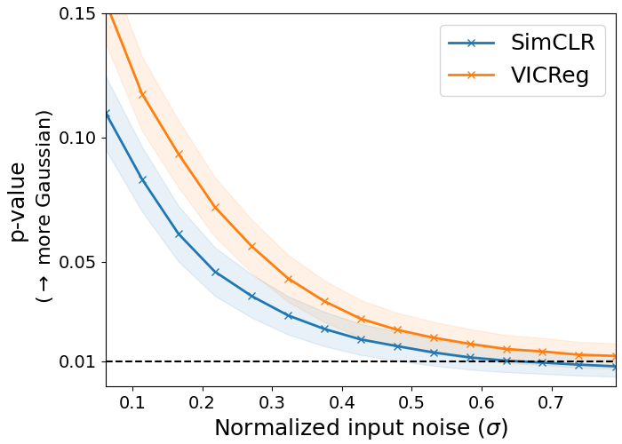
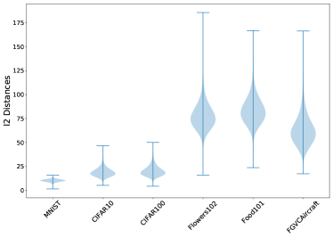
Figure 1: Left: The network output SSL training is more Gaussian for small input noise. The $p$-value of the normality test for different SSL models trained on CIFAR-10 for different input noise levels. The dashed line represents the point at which the null hypothesis (Gaussian distribution) can be rejected with $99\%$ confidence. Right: The Gaussians around each point are not overlapping The plots show the $l2$ distances between raw images for different datasets. As can be seen, the distances are largest for more complex real-world datasets.

4.1 An Information-Theoretic Perspective on VICReg

In the previous section, we derived an objective function based on information-theoretical principles. The “invariance term” in LABEL:eq:obj is similar to the invariance loss of VICReg. However, computing the regularization term—and $H(Z)$ in particular—is challenging. Estimating the entropy of random variables is a classic problem in information theory, with the Gaussian mixture density being a popular representation. However, there is no closed-form solution to the differential entropy of Gaussian mixtures. Approximations, including loose upper and lower bounds (Huber et al., 2008) and Monte Carlo sampling, exist in the literature. Unfortunately, Monte Carlo sampling is computationally expensive and requires many samples in high dimensions (Brewer, 2017).

One of the simplest and straightforward approaches to approximating the entropy is to capture the first two moments of the distribution, which provides an upper bound on the entropy. However, minimizing an upper bound means that there is no guarantee that the original objective is being optimized. In practice, there have been cases where successful results have been achieved by minimizing an upper bound (Martinez et al., 2021; Nowozin et al., 2016). However, this may cause instability in the training process. For a detailed discussion and results on different entropy estimators, see Section 5. Letting $\Sigma_{Z}$ be the covariance matrix of $Z$, we will use the first two moments to approximate the entropy we wish to maximize. This way, we obtain the approximation

$$L\approx\sum_{n=1}^{N}{\log\frac{|\Sigma_{Z}|}{|\Sigma(x_{i})|\cdot|\Sigma(x_{i}^{\prime})|}}-{\frac{1}{2}(\mu(x)-\mu(x^{\prime}))^{2}}.$$ (15)

A standard fact in linear algebra is that the determinant of a matrix is the product of its eigenvalues. Therefore, maximizing the sum of the log eigenvalues implies maximizing the log determinant of $Z$. Many works have considered this problem (Giles, 2008; Ionescu et al., 2015; Dang et al., 2018). One approach is to find the solutions using the eigendecomposition, which leads to numerical instability (Dang et al., 2018). An alternative approach is to diagonalize the covariance matrix and increase its diagonal elements. Because the eigenvalues of a diagonal matrix are the diagonal entries, increasing the sum of the log-diagonal terms is equivalent to increasing the sum of the log eigenvalues. One way to do this is to push the off-diagonal terms of $\Sigma_{Z}$ to be zero and maximize the sum of its log diagonal. This can be done using the covariance term of VICReg. Even though this approach is simple and efficient, the values on the diagonal may become close to zero, which may cause instability when we calculate the logarithm. Therefore, we use an upper bound and calculate the sum of the diagonal elements directly, which is the variance term of VICReg. In conclusion, we see the connection between the information-theoretic objective and the three terms of CIVReg. An exciting research direction is to maximize the eigenvalues of $Z$ using more sophisticated methods, such as using a differential expression for eigendecomposition.

4.2 Validation of Assumptions

Based on the theory outlined in Section 3.3, the conditional output density $p_{\bm{z}|x=i}$ can be reduced to a single Gaussian with decreasing input noise. To validate this, we used a ResNet-18 model trained with either SimCLR or VICReg objectives on the CIFAR-10 and CIFAR-100 datasets (Krizhevsky, 2009). We sampled 512 Gaussian samples for each image from the test dataset, and analyzed whether each sample remained Gaussian in the penultimate layer of the DNN. We then used the D’Agostino and Pearson’s test (D’Agostino, 1971) to determine the validity of this assumption. Figure 1 (left) shows the $p$-value as a function of the normalized standard deviation. For small noise, we can reject the hypothesis that the conditional output density of the network is not Gaussian with a probability of $85\%$ for VICReg. However, as the input noise increases, the network’s output becomes less Gaussian and even for the small noise regime, there is a $15\%$ chance of a Type I error.

Next, to confirm our assumption that the model of the data distribution has non-overlapping effective support, we calculated the distribution of pairwise $l_{2}$ distances between images for seven datasets: MNIST, CIFAR10, CIFAR100, Flowers102, Food101, FGVAircaft. Figure 1 (right) shows that even for raw pixels, the pairwise distances are far from zero, which means that we can use a small Gaussian around each point without overlapping. Therefore, the effective support of these datasets is non-overlapping, and our assumption is realistic.

5 Self-Supervised Learning via Mutual Information Maximization

Implementing Equation 12 in practice requires various “design choices.” As demonstrated in Section 5, VICReg uses an approximation of the entropy that is based on certain assumptions. Next, we examine different ways to implement the information-based objective by comparing VICReg to other methods such as contrastive learning SSL methods such as SimCLR and non-contrastive methods like BYOL and SimSiam. We will analyze their assumptions and the differences in their approaches to implementing the information maximization objective. Based on our analysis, we will suggest new objective functions that incorporate more recent information and entropy estimators from the information theory literature. This will allow us to further improve the performance of SSL and to better understand their underlying learning mechanisms.

5.1 VICReg vs. SimCLR

Contrastive Learning with SimCLR.

Lee et al. (2021b) connect the SimCLR objective (Chen et al., 2020) to the variational bound on the information between representations by using the von Mises-Fisher distribution as the conditional variational family. By applying our analysis for information in deterministic networks with their work, we can compare the differences between SimCLR and VICReg, and identify two main differences: (i) Conditional distribution: SimCLR assumes a von Mises-Fisher distribution for the encoder, while VICReg assumes a Gaussian distribution. (ii) Entropy estimation: The entropy term in SimCLR is approximate and based on the finite sum of the input samples. In contrast, VICReg estimates the entropy of $Z$ solely based on the second moment. Creating self-supervised methods that combine these two differences would be an interesting future research direction.

Empirical comparison.

As we saw in previous sections, the different methods use different objective functions to optimize the entropy of their representation. Next, we compare the SSL methods and check directly their entropy. To do so, we trained ResNet-18 architecture (He et al., 2016) on CIFAR-10 (Krizhevsky et al., 2009) for VICReg, SimCLR and BYOL. we used the pairwise distances entropy estimator based on the distances of the individual mixture component (Kolchinsky and Tracey, 2017). Even though this quantity is just an estimator for the entropy, it is shown as a tight estimator and is directly optimized by neither one of the methods. Therefore, we can treat it as a outsource validation of the entropy for the different methods. For more details on this and other entropy estimators see Section 5.2. In Figure 2, we see that, as expected from our analysis before, all the entropy decreased during the training for all the methods. Additionally, we see that SimCLR has the lowest entropy during the training, while VICReg has the highest one.

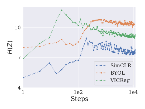
Figure 2: The entropy for the SSL models VICReg decreased during the training. The entropy (measured by the LogDet Entropy estimator) as a function of the number of steps during training for VICReg and SimCLR and BYOL. Additionally, SimCLR entropy estimation is tighter compared to the others.

5.2 Alternative Entropy Estimators

In Section 5.1, we discussed existing methods that use an approximation to the entropy. Next, we suggest combining the invariance term of these methods with plug-in methods for optimizing the entropy.

Entropy estimators.

The VICReg objective aims to approximate the log determinate of the empirical covariance matrix by using diagonal terms. However, as discussed in Section 4.1, this estimator can be problematic. Instead, we can plug in different entropy estimators. One such option is the LogDet Entropy Estimator (Zhouyin and Liu, 2021), which provides a tighter upper bound. This estimator uses the differential entropy $\alpha$ order entropy with scaled noise and was previously demonstrated as a tight estimator for high-dimensional features and robust to random noise. However, since the estimator is an upper bound on the entropy, we are not guaranteed to optimize the original objective when maximizing this upper bound. To address this problem, we also use a lower bound estimator, which is based on the pairwise distances of the individual mixture component (Kolchinsky and Tracey, 2017). For this family, a pairwise-distance function between component densities is defined for each member. These estimators are computationally efficient, as long as the pairwise-distance function and the entropy of each component distribution are easy to compute. They are continuous and smooth (and therefore useful for optimization problems) and converge to the exact solution when the component distributions are grouped into well-separated clusters. These proposed methods are compared with VICReg, SimCLR (Chen et al., 2020), and Barlow Twin (Zbontar et al., 2021).

Setup.

Our experiments are conducted on CIFAR-10 (Krizhevsky et al., 2009). A ResNet-18 architecture (He et al., 2016) is used as the backbone. We use linear evaluation for the quality of the representation. For full details, see Appendix H.

Results.

It can be seen from LABEL:tab:results that the proposed estimators outperform both the original VICReg and SimCLR as well as Barlow Twin. By estimating the entropy with a more accurate estimator, we can improve the results of VICReg, and the pairwise distance estimator, which is a lower bound, achieves the best results. This aligns with the theory that we want to maximize a lower bound on true entropy. The results of our study suggest that a smart selection of entropy estimators, inspired by our framework, leads to better results.

6 Information Maximization for VICReg and Downstream Generalization

In the previous sections, we showed the connection between information-theoretic principles and the VICReg objective. Next, we will connect this objective and the information-theoretic principles to the downstream generalization of VICReg by deriving a downstream generalization bound. Together with the results in the previous sections, this relates generalization in VICReg to information maximization and implicit regularization.

Notation.

Consider input points $x$, outputs $y\in\mathbb{R}^{r}$, labeled training data $S=((x_{i},y_{i}))_{i=1}^{n}$ of size $n$ and unlabeled training data ${\bar{S}}=((x^{+}_{i},x^{++}_{i}))_{i=1}^{m}$ of size $m$, where $x^{+}_{i}$ and $x^{++}_{i}$ share the same (unknown) label. With the unlabeled training data, we define the invariance loss

$$\SwapAboveDisplaySkip I_{{\bar{S}}}(f_{\theta})=\frac{1}{m}\sum_{i=1}^{m}\|f_{\theta}(x^{+}_{i})-f_{\theta}(x^{++}_{i})\|$$ (16)

where $f_{\theta}$ is the trained representation on the unlabeled data ${\bar{S}}$. We define a labeled loss $\ell_{x,y}(w)=\|Wf_{\theta}(x)-y\|$ where $w=\operatorname{vec}[W]\in\mathbb{R}^{dr}$ is the vectorization of the matrix $W\in\mathbb{R}^{r\times d}$. Let $w_{S}=\operatorname{vec}[W_{S}]$ be the minimum norm solution as $W_{S}=\mathop{\mathrm{minimize}}_{W^{\prime}}\|W^{\prime}\|_{F}$ such that

$$\SwapAboveDisplaySkip W^{\prime}\in\operatorname*{arg\,min}_{W}\frac{1}{n}\sum_{i=1}^{n}\|Wf_{\theta}(x_{i})-y_{i}\|^{2}.$$ (17)

We also define the representation matrices

$${Z_{S}}=[f(x_{1}),\dots,f(x_{n})]\in\mathbb{R}^{d\times n}\qquad\text{and}\qquad{Z_{\bar{S}}}=[f(x^{+}_{1}),\dots,f(x^{+}_{m})]\in\mathbb{R}^{d\times m},$$

and the projection matrices

$$\mathbf{P}_{Z_{S}}=I-{Z_{S}}^{\top}({Z_{S}}{Z_{S}}^{\top})^{\dagger}{Z_{S}}\qquad\text{and}\qquad\mathbf{P}_{Z_{\bar{S}}}=I-{Z_{\bar{S}}}^{\top}({Z_{\bar{S}}}{Z_{\bar{S}}}^{\top})^{\dagger}{Z_{\bar{S}}}.$$

We define the label matrix $Y_{S}=[y_{1},\dots,y_{n}]^{\top}\in\mathbb{R}^{n\times r}$ and the unknown label matrix $Y_{{\bar{S}}}=[y^{+}_{1},\dots,y^{+}_{m}]^{\top}\in\mathbb{R}^{m\times r}$, where $y^{+}_{i}$ is the unknown label of $x^{+}_{i}$. Let $\mathcal{F}$ be a hypothesis space of $f_{\theta}$. For a given hypothesis space $\mathcal{F}$, we define the normalized Rademacher complexity

$$\tilde{\mathcal{R}}_{m}(\mathcal{F})=\frac{1}{\sqrt{m}}\mathbb{E}_{{\bar{S}},\xi}\left[\sup_{f\in\mathcal{F}}\sum_{i=1}^{m}\xi_{i}\|f(x^{+}_{i})-f(x^{++}_{i})\|\right],$$

where $\xi_{1},\dots,\xi_{m}$ are independent uniform random variables taking values in $\{-1,1\}$. It is normalized such that $\tilde{\mathcal{R}}_{m}(\mathcal{F})=O(1)$ as $m\rightarrow\infty$ for typical choices of hypothesis spaces $\mathcal{F}$, including deep neural networks (Bartlett et al., 2017; Kawaguchi et al., 2018).

6.1 A Generalization Bound for Variance-Invariance-Covariance Regularization

Theorem 2 shows that VICReg improves generalization on supervised downstream tasks. More cpecifically, minimizing the unlabeled invariance loss while controlling the covariance ${Z_{\bar{S}}}{Z_{\bar{S}}}^{\top}$ and the complexity of representations $\tilde{\mathcal{R}}_{m}(\mathcal{F})$ minimizes the expected labeled loss:

Theorem 2

(Informal version). For any $\delta>0$, with probability at least $1-\delta$,

$$\begin{split}&\mathbb{E}_{x,y}[\ell_{x,y}(w_{S})]\leq I_{{\bar{S}}}(f_{\theta})+\frac{2}{\sqrt{m}}\|\mathbf{P}_{Z_{\bar{S}}}Y_{\bar{S}}\|_{F}+\frac{1}{\sqrt{n}}\|\mathbf{P}_{Z_{S}}Y_{S}\|_{F}+\frac{2\tilde{\mathcal{R}}_{m}(\mathcal{F})}{\sqrt{m}}+\mathcal{Q}_{m,n},\end{split}$$ (18)

where $\mathcal{Q}_{m,n}=O(G\sqrt{\ln(1/\delta)/m}+\sqrt{\ln(1/\delta)/n})\rightarrow 0$ as $m,n\rightarrow\infty$. In $\mathcal{Q}_{m,n}$, the value of $G$ for the term decaying at the rate $1/\sqrt{m}$ depends on the hypothesis space of $f_{\theta}$ and $w$ whereas the term decaying at the rate $1/\sqrt{n}$ is independent of any hypothesis space.

Proof  The complete version of Theorem 2 and its proof are presented in Appendix I.  

The term $\|\mathbf{P}_{Z_{\bar{S}}}Y_{\bar{S}}\|_{F}$ in Theorem 2 contains the unobservable label matrix $Y_{\bar{S}}$. However, we can minimize this term by using $\|\mathbf{P}_{Z_{\bar{S}}}Y_{\bar{S}}\|_{F}\leq\|\mathbf{P}_{Z_{\bar{S}}}\|_{F}\|Y_{\bar{S}}\|_{F}$ and by minimizing $\|\mathbf{P}_{Z_{\bar{S}}}\|_{F}$. The factor $\|\mathbf{P}_{Z_{\bar{S}}}\|_{F}$ is minimized when the rank of the covariance ${Z_{\bar{S}}}{Z_{\bar{S}}}^{\top}$ is maximized. Since a strictly diagonally dominant matrix is non-singular, this can be enforced by maximizing the diagonal entries while minimizing the off-diagonal entries, as is done in VICReg. For example, if $d\geq n$, then $\|\mathbf{P}_{Z_{\bar{S}}}\|_{F}=0$ when the covariance ${Z_{\bar{S}}}{Z_{\bar{S}}}^{\top}$ is of full rank.

The term $\|\mathbf{P}_{Z_{S}}Y_{S}\|_{F}$ contains only observable variables, and we can directly measure the value of this term using training data. In addition, the term $\|\mathbf{P}_{Z_{S}}Y_{S}\|_{F}$ is also minimized when the rank of the covariance ${Z_{S}}{Z_{S}}^{\top}$ is maximized. Since the covariances ${Z_{S}}{Z_{S}}^{\top}$ and ${Z_{\bar{S}}}{Z_{\bar{S}}}^{\top}$ concentrate to each other via concentration inequalities with the error in the order of $O(\sqrt{(\ln(1/\delta))/n}+\tilde{\mathcal{R}}_{m}(\mathcal{F})\sqrt{(\ln(1/\delta))/m})$, we can also minimize the upper bound on $\|\mathbf{P}_{Z_{S}}Y_{S}\|_{F}$ by maximizing the diagonal entries of ${Z_{\bar{S}}}{Z_{\bar{S}}}^{\top}$ while minimizing its off-diagonal entries, as is done in VICReg.

Thus, VICReg can be understood as a method to minimize the generalization bound in Theorem 2 by minimizing the invariance loss while controlling the covariance ${Z_{\bar{S}}}{Z_{\bar{S}}}^{\top}$ to minimize the label-agnostic upper bounds on $\|\mathbf{P}_{Z_{\bar{S}}}Y_{\bar{S}}\|_{F}$ and $\|\mathbf{P}_{Z_{S}}Y_{S}\|_{F}$. If we know partial information about the label $Y_{\bar{S}}$ of the unlabeled data, we can use it to minimize $\|\mathbf{P}_{Z_{\bar{S}}}Y_{\bar{S}}\|_{F}$ and $\|\mathbf{P}_{Z_{S}}Y_{S}\|_{F}$ directly. This direction can be used to improve VICReg in future work for the partially observable setting.

6.2 Comparison of Generalization Bounds

The SimCLR generalization bound (Saunshi et al., 2019) requires the number of label classes to go infinity to close the generalization gap, whereas the VICReg bound in Theorem 2 does not require the number of label classes to approach infinity for the generalization gap to go to zero. This reflects the fact that, unlike SimCLR, VICReg does not use negative pairs and thus does not use a loss function that is based on the implicit expectation that the labels of a negative pair $(y^{+},y^{-})$ are different. Another difference is that our VICReg bound improves as $n$ increases, while the previous bound of SimCLR (Saunshi et al., 2019) does not depend on $n$. This is because Saunshi et al. (2019) assume partial access to the true distribution $p(x\mid y)$ per class for setting $W$, which removes the importance of labeled data size $n$ and is not assumed in our study.

Consequently, the generalization bound in Theorem 2 provides a new insight for VICReg regarding the ratio of the effects of $m$ v.s. $n$ through $G\sqrt{\ln(1/\delta)/m}+\sqrt{\ln(1/\delta)/n}$. Finally, Theorem 2 also illuminates the advantages of VICReg over standard supervised training. That is, with standard training, the generalization bound via the Rademacher complexity requires the complexities of hypothesis spaces, $\tilde{\mathcal{R}}_{n}(\mathcal{W})/\sqrt{n}$ and $\tilde{\mathcal{R}}_{n}(\mathcal{F})/\sqrt{n}$, with respect to the size of labeled data $n$, instead of the size of unlabeled data $m$.

Thus, Theorem 2 shows that using self-supervised learning, we can replace all the complexities of hypothesis spaces in terms of $n$ with those in terms of $m$. Since the number of unlabeled data points is typically much larger than the number of labeled data points, this illuminates the benefit of self-supervised learning.

6.3 Understanding Theorem 2 via Mutual Information Maximization

Theorem 2 together with the result of the previous section shows that, for generalization in the downstream task, it is helpful to maximize the mutual information $I(Z;X^{\prime})$ in SSL via minimizing the invariance loss $I_{{\bar{S}}}(f_{\theta})$ while controlling the covariance ${Z_{\bar{S}}}{Z_{\bar{S}}}^{\top}$. The term $2\tilde{\mathcal{R}}_{m}(\mathcal{F})/\sqrt{m}$ captures the importance of controlling the complexity of the representations $f_{\theta}$. To understand this term further in terms of mutual information, let us consider a discretization of the parameter space of $\mathcal{F}$ to have finite $|\mathcal{F}|<\infty$ (indeed, a computer always implements some discretization of continuous variables). Then, by Massart’s Finite Class Lemma, we have that $\tilde{\mathcal{R}}_{m}(\mathcal{F})\leq C\sqrt{\ln|\mathcal{F}|}$ for some constant $C>0$. Moreover, Shwartz-Ziv (2022) shows that we can approximate $\ln|\mathcal{F}|$ by $2^{I(Z;X)}$. Thus, in Theorem 2, the term $I_{{\bar{S}}}(f_{\theta})+\frac{2}{\sqrt{m}}\|\mathbf{P}_{Z_{\bar{S}}}Y_{\bar{S}}\|_{F}+\frac{1}{\sqrt{n}}\|\mathbf{P}_{Z_{S}}Y_{S}\|_{F}$ corresponds to $I(Z;X^{\prime})$ while the term of $2\tilde{\mathcal{R}}_{m}(\mathcal{F})/\sqrt{m}$ corresponds to $I(Z;X)$. Recall that the information can be decomposed as

$$I(Z;X)=I(Z;X^{\prime})+I(Z;X|X^{\prime}).$$ (19)

where we want to maximize the predictive information $I(Z;X^{\prime})$, while minimizing $I(Z;X)$ (Federici et al., 2019; Shwartz-Ziv and Tishby, 2017a). Thus, to improve generalization, we also need to control $2\tilde{\mathcal{R}}_{m}(\mathcal{F})/\sqrt{m}$ to restrict the superfluous information $I(Z;X|X^{\prime})$, in addition to minimizing $I_{{\bar{S}}}(f_{\theta})+\frac{2}{\sqrt{m}}\|\mathbf{P}_{Z_{\bar{S}}}Y_{\bar{S}}\|_{F}+\frac{1}{\sqrt{n}}\|\mathbf{P}_{Z_{S}}Y_{S}\|_{F}$ that corresponded to maximize the predictive information $I(Z;X^{\prime})$. Although we can explicitly add regularization on $I(Z;X|X^{\prime})$ to control $2\tilde{\mathcal{R}}_{m}(\mathcal{F})/\sqrt{m}$, it is possible that $I(Z;X|X^{\prime})$ and $2\tilde{\mathcal{R}}_{m}(\mathcal{F})/\sqrt{m}$ are implicitly regularized via implicit bias through e design choises (Gunasekar et al., 2017; Soudry et al., 2018; Gunasekar et al., 2018). Thus, Theorem 2 connects the information-theoretic understanding of VICReg with the probabilistic guarantee on downstream generalization.

7 Conclusions

In this study, we examined Variance-Invariance-Covariance Regularization for self-supervised learning from an information-theoretic perspective. By transferring the required stochasticity required for an information-theoretic analysis to the input distribution, we showed how the VICReg objective can be derived from information-theoretic principles, used this perspective to highlight assumptions implicit in the VICReg objective, derived a VICReg generalization bound for downstream tasks, and related it to information maximization.

Finally, we built on the insights from our analysis to propose a new VICReg-style SSL objective. Our probabilistic guarantee suggests that VICReg can be further improved for the settings of partial label information by aligning the covariance matrix with the partially observable label matrix, which opens up several avenues for future work, including the design of improved estimators for information-theoretic quantities and investigations into the suitability of different SSL methods for specific data characteristics.

Supplementary Material

Appendix A Lower bounds on $\mathbb{E}_{x^{\prime}}\left[\log q(z|x^{\prime})\right]$

In this section of the supplementary material, we present the full derivation of the lower bound on $\mathbb{E}_{x^{\prime}}\left[\log q(z|x^{\prime})\right]$. Because $Z^{\prime}|X^{\prime}$ is a Gaussian, we can write it as $Z^{\prime}=\mu(x^{\prime})+L(x^{\prime})\epsilon$ where $\epsilon\sim\mathcal{N}(0,1)$ and $L(x^{\prime})^{T}L(x^{\prime})=\Sigma(x^{\prime})$. Now, setting $\Sigma_{r}=I$, will give us:

$$\begin{split}&\mathbb{E}_{x^{\prime}}\left[\log q(z|x^{\prime})\right]\\ \geq&\mathbb{E}_{z^{\prime}|x^{\prime}}\left[\log q(z|z^{\prime})\right]\end{split}$$ (A.1)

$$= \mathbb{E}_{z^{\prime}|x^{\prime}}\left[\frac{d}{2}\log 2\pi-\frac{1}{2}\left(z-z^{\prime}\right)^{T}\left(I)\right)^{-1}\left(z-z^{\prime}\right)\right]$$ (A.2)

$$= \frac{d}{2}\log 2\pi-\frac{1}{2}\mathbb{E}_{z^{\prime}\mid x^{\prime},}\left[\left(z-z^{\prime}\right)^{2}\right]$$ (A.3)

$$= \frac{d}{2}\log 2\pi-\frac{1}{2}\mathbb{E}_{\epsilon}\left[\left(z-\mu(x^{\prime})-L(x^{\prime})\epsilon\right)^{2}\right]$$ (A.4)

$$= \frac{d}{2}\log 2\pi-\frac{1}{2}\mathbb{E}_{\epsilon}\left[\left(z-\mu(x^{\prime})\right)^{2}-2\left(z-\mu(x^{\prime})*L(x^{\prime})\epsilon\right)+\left(\left(L(x^{\prime})\epsilon\right)^{T}\left(L(x^{\prime})\epsilon\right)\right)\right]$$ (A.5)

$$= \frac{d}{2}\log 2\pi-\frac{1}{2}\mathbb{E}_{\epsilon}\left[\left(z-\mu(x^{\prime})\right)^{2}\right]+\left(z-\mu(x^{\prime})L(x^{\prime})\right)\mathbb{E}_{\epsilon}\left[\epsilon\right]-\frac{1}{2}\mathbb{E}_{\epsilon}\left[\epsilon^{T}L(x^{\prime})^{T}L(x^{\prime})\epsilon\right]$$ (A.6)

$$= \frac{d}{2}\log 2\pi-\frac{1}{2}\left(z-\mu(x^{\prime})\right)^{2}-\frac{1}{2}Tr\log\Sigma(x^{\prime})$$ (A.7)

where $\mathbb{E}_{x^{\prime}}\left[\log q(z|x^{\prime})\right]=\mathbb{E}_{x^{\prime}}\left[\log\mathbb{E}_{z^{\prime}|x^{\prime}}\left[q(z|z^{\prime})\right]\right]\geq\mathbb{E}_{z^{\prime}}\left[\log q(z|z^{\prime})\right]$ by Jensen’s inequality, $\mathbb{E}_{\epsilon}[\epsilon]=0$ and $\mathbb{E}_{\epsilon}\left[\epsilon\left(L(x^{\prime})^{T}L(x^{\prime}\right)\epsilon\right]=Tr\log\Sigma(x^{\prime})$ by the Hutchinson’s estimator.

$$\mathbb{E}_{z|x}\left[\mathbb{E}_{z^{\prime}|x^{\prime}}\left[\log q(z|z^{\prime})\right]\right]= \mathbb{E}_{z|x}\left[\frac{d}{2}\log 2\pi-\frac{1}{2}\left(z-\mu(x^{\prime})\right)^{2}-\frac{1}{2}Tr\log\Sigma(x^{\prime})\right]$$ (A.8)

$$= \frac{d}{2}\log 2\pi-\frac{1}{2}\mathbb{E}_{z|x}\left[\left(z-\mu(x^{\prime})\right)^{2}\right]-\frac{1}{2}Tr\log\Sigma(x^{\prime})$$ (A.9)

$$= \frac{d}{2}\log 2\pi-\frac{1}{2}\mathbb{E}_{\epsilon}\left[\left(\mu(x)+L(x)\epsilon-\mu(x^{\prime})\right)^{2}\right]-\frac{1}{2}Tr\log\Sigma(x^{\prime})$$ (A.10)

$$\begin{split}=&\frac{d}{2}\log 2\pi-\frac{1}{2}\mathbb{E}_{\epsilon}\left[\left(\mu(x)-\mu(x^{\prime})\right)^{2}\right]+\mathbb{E}_{\epsilon}\left[\left(\mu(x)-\mu(x^{\prime})\right)L(x)\epsilon\right]\\ &-\frac{1}{2}\mathbb{E}_{\epsilon}\left[\epsilon^{T}L(x)^{T}L(x)\epsilon\right]-\frac{1}{2}Tr\log\Sigma(x^{\prime})\end{split}$$ (A.11)

$$= \frac{d}{2}\log 2\pi-\frac{1}{2}\left(\mu(x)-\mu(x^{\prime})\right)^{2}-\frac{1}{2}Tr\log\Sigma(x)-\frac{1}{2}Tr\log\Sigma(x^{\prime})$$ (A.12)

$$= \frac{d}{2}\log 2\pi-\frac{1}{2}\left(\mu(x)-\mu(x^{\prime})\right)^{2}-\frac{1}{2}\log\left(|\Sigma(x)|\cdot|\Sigma(x^{\prime})|\right)$$ (A.13)

Appendix B Data Distribution after Deep Network Transformation

Theorem 3

Given the setting of eq. 8 the unconditional DNN output density denoted as $Z$ approximates (given the truncation of the Gaussian on its effective support that is included within a single region $\omega$ of the DN’s input space partition) a mixture of the affinely transformed distributions $\bm{x}|\bm{x}^{*}_{n(\bm{x})}$ e.g. for the Gaussian case

$$Z\sim\sum_{n=1}^{N}\mathcal{N}\left(\bm{A}_{\omega(\bm{x}^{*}_{n})}\bm{x}^{*}_{n}+\bm{b}_{\omega(\bm{x}^{*}_{n})},\bm{A}^{T}_{\omega(\bm{x}^{*}_{n})}\Sigma_{\bm{x}^{*}_{n}}\bm{A}_{\omega(\bm{x}^{*}_{n})}\right)^{T=n},$$

where $\omega(\bm{x}^{*}_{n})=\omega\in\Omega\iff\bm{x}^{*}_{n}\in\omega$ is the partition region in which the prototype $\bm{x}^{*}_{n}$ lives in.

Proof  We know that If $\int_{\omega}p(\bm{x}|\bm{x}^{*}_{n(\bm{x})})d\bm{x}\approx 1$ then $f$ is linear within the effective support of $p$. Therefore, any sample from $p$ will almost surely lie within a single region $\omega\in\Omega$ and therefore the entire mapping can be considered linear with respect to $p$. Thus, the output distribution is a linear transformation of the input distribution based on the per-region affine mapping.  

Appendix C Generalization Bound

The following theorem is the complete version of Theorem 2:

Theorem 4

For any $\delta>0$, with probability at least $1-\delta$, the following holds:

$$\mathbb{E}_{x,y}[\ell_{x,y}(w_{S})]\leq cI_{{\bar{S}}}(f_{\theta})+\frac{2}{\sqrt{m}}\|\mathbf{P}_{Z_{\bar{S}}}Y_{\bar{S}}\|_{F}+\frac{1}{\sqrt{n}}\|\mathbf{P}_{Z_{S}}Y_{S}\|_{F}+Q_{m,n},$$ (C.14)

where

$$Q_{m,n} =c\left(\frac{2\tilde{\mathcal{R}}_{m}(\mathcal{F})}{\sqrt{m}}+\tau\sqrt{\frac{\ln(3/\delta)}{2m}}+\tau_{{\bar{S}}}\sqrt{\frac{\ln(3/\delta)}{2n}}\right)$$

$$\quad+\kappa_{S}\sqrt{\frac{2\ln(6|\mathcal{Y}|/\delta)}{2n}}\sum_{y\in\mathcal{Y}}\left(\sqrt{{\hat{p}}(y)}+\sqrt{p(y)}\right)$$

$$\quad+\frac{4\mathcal{R}_{m}(\mathcal{W}\circ\mathcal{F})}{\sqrt{m}}+2\kappa\sqrt{\frac{\ln(4/\delta)}{2m}}+2\kappa_{{\bar{S}}}\sqrt{\frac{\ln(4/\delta)}{2n}}.$$

Proof  The complete proof is presented in Appendix C.1.  

The bound in the complete version of Theorem 4 is better than the one in the informal version of Theorem 2, because of the factor $c$. The factor $c$ measures the difference between the minimum norm solution $W_{S}$ of the labeled training data and the minimum norm solution $W_{\bar{S}}$ of the unlabeled training data. Thus, the factor $c$ also decreases towards zero as $n$ and $m$ increase. Moreover, if the labeled and unlabeled training data are similar, the value of $c$ is small, decreasing the generalization bound further, which makes sense. Thus, we can view the factor $c$ as a measure on the distance between the labeled training data and the unlabeled training data.

We obtain the informal version from the complete version of Theorem 2 by the following reasoning to simplify the notation in the main text. We have that $cI_{{\bar{S}}}(f_{\theta})+c\frac{2\tilde{\mathcal{R}}_{m}(\mathcal{F})}{\sqrt{m}}=I_{{\bar{S}}}(f_{\theta})+\frac{2\tilde{\mathcal{R}}_{m}(\mathcal{F})}{\sqrt{m}}+Q$, where $Q=(c-1)(I_{{\bar{S}}}(f_{\theta})+\frac{2\tilde{\mathcal{R}}_{m}(\mathcal{F})}{\sqrt{m}})\leq\varsigma\rightarrow 0$ as as $m,n\rightarrow\infty$, since $c\rightarrow 0$ as $m,n\rightarrow\infty$. However, this reasoning is used only to simplify the notation in the main text. The bound in the complete version of Theorem 2 is more accurate and indeed tighter than the one in the informal version.

In Theorem 2, $Q_{m,n}\rightarrow 0$ as $m,n\rightarrow\infty$ if $\frac{\tilde{\mathcal{R}}_{m}(\mathcal{F})}{\sqrt{m}}\rightarrow 0$ as $m\rightarrow\infty$. Indeed, this typically holds because $\tilde{\mathcal{R}}_{m}(\mathcal{F})=O(1)$ as $m\rightarrow\infty$ for typical choices of $\mathcal{F}$, including deep neural networks (Bartlett et al., 2017; Kawaguchi et al., 2018; Golowich et al., 2018) as well as other common machine learning models (Bartlett and Mendelson, 2002; Mohri et al., 2012; Shalev-Shwartz and Ben-David, 2014; Shwartz-Ziv et al., 2023).

C.1 Proof of Theorem 2

Proof [Proof of Theorem 2] Let $W=W_{S}$ where $W_{S}$ is the the minimum norm solution as $W_{S}=\mathop{\mathrm{minimize}}_{W^{\prime}}\|W^{\prime}\|_{F}$ s.t. $W^{\prime}\in\operatorname*{arg\,min}_{W}\frac{1}{n}\sum_{i=1}^{n}\|Wf_{\theta}(x_{i})-y_{i}\|^{2}$. Let $W^{*}=W_{\bar{S}}$ where $W_{\bar{S}}$ is the minimum norm solution as $W^{*}=W_{{\bar{S}}}=\mathop{\mathrm{minimize}}_{W^{\prime}}\|W^{\prime}\|_{F}$ s.t. $W^{\prime}\in\operatorname*{arg\,min}_{W}\frac{1}{m}\sum_{i=1}^{m}\|Wf_{\theta}(x^{+}_{i})-g^{*}(x^{+}_{i})\|^{2}$. Since $y=g^{*}(x)$,

$$y=g^{*}(x)\pm W^{*}f_{\theta}(x)=W^{*}f_{\theta}(x)+(g^{*}(x)-W^{*}f_{\theta}(x))=W^{*}f_{\theta}(x)+\varphi(x)$$

where $\varphi(x)=g^{*}(x)-W^{*}f_{\theta}(x)$. Define $L_{S}(w)=\frac{1}{n}\sum_{i=1}^{n}\|Wf_{\theta}(x_{i})-y_{i}\|$. Using these,

$$L_{S}(w) =\frac{1}{n}\sum_{i=1}^{n}\|Wf_{\theta}(x_{i})-y_{i}\|$$

$$=\frac{1}{n}\sum_{i=1}^{n}\|Wf_{\theta}(x_{i})-W^{*}f_{\theta}(x_{i})-\varphi(x_{i})\|$$

$$\geq\frac{1}{n}\sum_{i=1}^{n}\|Wf_{\theta}(x_{i})-W^{*}f_{\theta}(x_{i})\|-\frac{1}{n}\sum_{i=1}^{n}\|\varphi(x_{i})\|$$

$$=\frac{1}{n}\sum_{i=1}^{n}\|{\tilde{W}}f_{\theta}(x_{i})\|-\frac{1}{n}\sum_{i=1}^{n}\|\varphi(x_{i})\|$$

where ${\tilde{W}}=W-W^{*}$. We now consider new fresh samples ${\bar{x}}_{i}\sim\mathcal{D}_{y_{i}}$ for $i=1,\dots,n$ to rewrite the above further as:

$$L_{S}(w) \geq\frac{1}{n}\sum_{i=1}^{n}\|{\tilde{W}}f_{\theta}(x_{i})\pm{\tilde{W}}f_{\theta}({\bar{x}}_{i})\|-\frac{1}{n}\sum_{i=1}^{n}\|\varphi(x_{i})\|$$

$$=\frac{1}{n}\sum_{i=1}^{n}\|{\tilde{W}}f_{\theta}({\bar{x}}_{i})-({\tilde{W}}f_{\theta}({\bar{x}}_{i})-{\tilde{W}}f_{\theta}(x_{i}))\|-\frac{1}{n}\sum_{i=1}^{n}\|\varphi(x_{i})\|$$

$$\geq\frac{1}{n}\sum_{i=1}^{n}\|{\tilde{W}}f_{\theta}({\bar{x}}_{i})\|-\frac{1}{n}\sum_{i=1}^{n}\|{\tilde{W}}f_{\theta}({\bar{x}}_{i})-{\tilde{W}}f_{\theta}(x_{i})\|-\frac{1}{n}\sum_{i=1}^{n}\|\varphi(x_{i})\|$$

$$=\frac{1}{n}\sum_{i=1}^{n}\|{\tilde{W}}f_{\theta}({\bar{x}}_{i})\|-\frac{1}{n}\sum_{i=1}^{n}\|{\tilde{W}}(f_{\theta}({\bar{x}}_{i})-f_{\theta}(x_{i}))\|-\frac{1}{n}\sum_{i=1}^{n}\|\varphi(x_{i})\|$$

This implies that

$$\frac{1}{n}\sum_{i=1}^{n}\|{\tilde{W}}f_{\theta}({\bar{x}}_{i})\|\leq L_{S}(w)+\frac{1}{n}\sum_{i=1}^{n}\|{\tilde{W}}(f_{\theta}({\bar{x}}_{i})-f_{\theta}(x_{i}))\|+\frac{1}{n}\sum_{i=1}^{n}\|\varphi(x_{i})\|.$$

Furthermore, since $y=W^{*}f_{\theta}(x)+\varphi(x)$, by writing ${\bar{y}}_{i}=W^{*}f_{\theta}({\bar{x}}_{i})+\varphi({\bar{x}}_{i})$ (where ${\bar{y}}_{i}=y_{i}$ since ${\bar{x}}_{i}\sim\mathcal{D}_{y_{i}}$ for $i=1,\dots,n$),

$$\frac{1}{n}\sum_{i=1}^{n}\|{\tilde{W}}f_{\theta}({\bar{x}}_{i})\| =\frac{1}{n}\sum_{i=1}^{n}\|Wf_{\theta}({\bar{x}}_{i})-W^{*}f_{\theta}({\bar{x}}_{i})\|$$

$$=\frac{1}{n}\sum_{i=1}^{n}\|Wf_{\theta}({\bar{x}}_{i})-{\bar{y}}_{i}+\varphi({\bar{x}}_{i})\|$$

$$\geq\frac{1}{n}\sum_{i=1}^{n}\|Wf_{\theta}({\bar{x}}_{i})-{\bar{y}}_{i}\|-\frac{1}{n}\sum_{i=1}^{n}\|\varphi({\bar{x}}_{i})\|$$

Combining these, we have that

$$\frac{1}{n}\sum_{i=1}^{n}\|Wf_{\theta}({\bar{x}}_{i})-{\bar{y}}_{i}\| \leq L_{S}(w)+\frac{1}{n}\sum_{i=1}^{n}\|{\tilde{W}}(f_{\theta}({\bar{x}}_{i})-f_{\theta}(x_{i}))\|$$ (C.15)

$$\quad+\frac{1}{n}\sum_{i=1}^{n}\|\varphi(x_{i})\|+\frac{1}{n}\sum_{i=1}^{n}\|\varphi({\bar{x}}_{i})\|.$$

To bound the left-hand side of equation C.15, we now analyze the following random variable:

$$\mathbb{E}_{X,Y}[\|W_{S}f_{\theta}(X)-Y\|]-\frac{1}{n}\sum_{i=1}^{n}\|W_{S}f_{\theta}({\bar{x}}_{i})-{\bar{y}}_{i}\|,$$ (C.16)

where ${\bar{y}}_{i}=y_{i}$ since ${\bar{x}}_{i}\sim\mathcal{D}_{y_{i}}$ for $i=1,\dots,n$. Importantly, this means that as $W_{S}$ depends on $y_{i}$, $W_{S}$ depends on ${\bar{y}}_{i}$. Thus, the collection of random variables $\|W_{S}f_{\theta}({\bar{x}}_{1})-{\bar{y}}_{1}\|,\dots,\|W_{S}f_{\theta}(n_{n})-{\bar{y}}_{n}\|$ is not independent. Accordingly, we cannot apply standard concentration inequality to bound equation C.16. A standard approach in learning theory is to first bound equation C.16 by $\mathbb{E}_{x,y}\|W_{S}f_{\theta}(x)-y\|-\frac{1}{n}\sum_{i=1}^{n}\|W_{S}f_{\theta}({\bar{x}}_{i})-{\bar{y}}_{i}\|\leq\sup_{W\in\mathcal{W}}\mathbb{E}_{x,y}\|Wf_{\theta}(x)-y\|-\frac{1}{n}\sum_{i=1}^{n}\|Wf_{\theta}({\bar{x}}_{i})-{\bar{y}}_{i}\|$ for some hypothesis space $\mathcal{W}$ (that is independent of $S$) and realize that the right-hand side now contains the collection of independent random variables $\|Wf_{\theta}({\bar{x}}_{1})-{\bar{y}}_{1}\|,\dots,\|Wf_{\theta}(n_{n})-{\bar{y}}_{n}\|$ , for which we can utilize standard concentration inequalities. This reasoning leads to the Rademacher complexity of the hypothesis space $\mathcal{W}$. However, the complexity of the hypothesis space $\mathcal{W}$ can be very large, resulting into a loose bound. In this proof, we show that we can avoid the dependency on hypothesis space $\mathcal{W}$ by using a very different approach with conditional expectations to take care the dependent random variables $\|W_{S}f_{\theta}({\bar{x}}_{1})-{\bar{y}}_{1}\|,\dots,\|W_{S}f_{\theta}(n_{n})-{\bar{y}}_{n}\|$. Intuitively, we utilize the fact that for these dependent random variables, there are a structure of conditional independence, conditioned on each $y\in\mathcal{Y}$.

We first write the expected loss as the sum of the conditional expected loss:

$$\mathbb{E}_{X,Y}[\|W_{S}f_{\theta}(X)-Y\|] =\sum_{y\in\mathcal{Y}}\mathbb{E}_{X,Y}[\|W_{S}f_{\theta}(X)-Y\|\mid Y=y]{\mathbb{P}}(Y=y)$$

$$=\sum_{y\in\mathcal{Y}}\mathbb{E}_{X_{y}}[\|W_{S}f_{\theta}(X_{y})-y\|]{\mathbb{P}}(Y=y),$$

where $X_{y}$ is the random variable for the conditional with $Y=y$. Using this, we decompose equation C.16 into two terms:

$$\mathbb{E}_{X,Y}[\|W_{S}f_{\theta}(X)-Y\|]-\frac{1}{n}\sum_{i=1}^{n}\|W_{S}f_{\theta}({\bar{x}}_{i})-{\bar{y}}_{i}\|$$ (C.17)

$$=\left(\sum_{y\in\mathcal{Y}}\mathbb{E}_{X_{y}}[\|W_{S}f_{\theta}(X_{y})-y\|]\frac{|\mathcal{I}_{y}|}{n}-\frac{1}{n}\sum_{i=1}^{n}\|W_{S}f_{\theta}({\bar{x}}_{i})-{\bar{y}}_{i}\|\right)$$

$$\quad+\sum_{y\in\mathcal{Y}}\mathbb{E}_{X_{y}}[\|W_{S}f_{\theta}(X_{y})-y\|]\left({\mathbb{P}}(Y=y)-\frac{|\mathcal{I}_{y}|}{n}\right),$$

where

$$\mathcal{I}_{y}=\{i\in[n]:y_{i}=y\}.$$

The first term in the right-hand side of equation C.17 is further simplified by using

$$\frac{1}{n}\sum_{i=1}^{n}\|W_{S}f_{\theta}({\bar{x}}_{i})-{\bar{y}}_{i}\|=\frac{1}{n}\sum_{y\in\mathcal{Y}}\sum_{i\in\mathcal{I}_{y}}\|W_{S}f_{\theta}({\bar{x}}_{i})-y\|,$$

as

$$\sum_{y\in\mathcal{Y}}\mathbb{E}_{X_{y}}[\|W_{S}f_{\theta}(X_{y})-y\|]\frac{|\mathcal{I}_{y}|}{n}-\frac{1}{n}\sum_{i=1}^{n}\|W_{S}f_{\theta}({\bar{x}}_{i})-{\bar{y}}_{i}\|$$

$$=\frac{1}{n}\sum_{y\in{\tilde{\mathcal{Y}}}}|\mathcal{I}_{y}|\left(\mathbb{E}_{X_{y}}[\|W_{S}f_{\theta}(X_{y})-y\|]-\frac{1}{|\mathcal{I}_{y}|}\sum_{i\in\mathcal{I}_{y}}\|W_{S}f_{\theta}({\bar{x}}_{i})-y\|\right),$$

where ${\tilde{\mathcal{Y}}}=\{y\in\mathcal{Y}:|\mathcal{I}_{y}|\neq 0\}$. Substituting these into equation equation C.17 yields

$$\mathbb{E}_{X,Y}[\|W_{S}f_{\theta}(X)-Y\|]-\frac{1}{n}\sum_{i=1}^{n}\|W_{S}f_{\theta}({\bar{x}}_{i})-{\bar{y}}_{i}\|$$ (C.18)

$$=\frac{1}{n}\sum_{y\in{\tilde{\mathcal{Y}}}}|\mathcal{I}_{y}|\left(\mathbb{E}_{X_{y}}[\|W_{S}f_{\theta}(X_{y})-y\|]-\frac{1}{|\mathcal{I}_{y}|}\sum_{i\in\mathcal{I}_{y}}\|W_{S}f_{\theta}({\bar{x}}_{i})-y\|\right)$$

$$\quad+\sum_{y\in\mathcal{Y}}\mathbb{E}_{X_{y}}[\|W_{S}f_{\theta}(X_{y})-y\|]\left({\mathbb{P}}(Y=y)-\frac{|\mathcal{I}_{y}|}{n}\right)$$

Importantly, while $\|W_{S}f_{\theta}({\bar{x}}_{1})-{\bar{y}}_{1}\|,\dots,\|W_{S}f_{\theta}({\bar{x}}_{n})-{\bar{y}}_{n}\|$ on the right-hand side of equation C.18 are dependent random variables, $\|W_{S}f_{\theta}({\bar{x}}_{1})-y\|,\dots,\|W_{S}f_{\theta}({\bar{x}}_{n})-y\|$ are independent random variables since $W_{S}$ and ${\bar{x}}_{i}$ are independent and $y$ is fixed here. Thus, by using Hoeffding’s inequality (Lemma 1), and taking union bounds over $y\in{\tilde{\mathcal{Y}}}$, we have that with probability at least $1-\delta$, the following holds for all $y\in{\tilde{\mathcal{Y}}}$:

$$\mathbb{E}_{X_{y}}[\|W_{S}f_{\theta}(X_{y})-y\|]-\frac{1}{|\mathcal{I}_{y}|}\sum_{i\in\mathcal{I}_{y}}\|W_{S}f_{\theta}({\bar{x}}_{i})-y\|\leq\kappa_{S}\sqrt{\frac{\ln(|{\tilde{\mathcal{Y}}}|/\delta)}{2|\mathcal{I}_{y}|}}.$$

This implies that with probability at least $1-\delta$,

$$\frac{1}{n}\sum_{y\in{\tilde{\mathcal{Y}}}}|\mathcal{I}_{y}|\left(\mathbb{E}_{X_{y}}[\|W_{S}f_{\theta}(X_{y})-y\|]-\frac{1}{|\mathcal{I}_{y}|}\sum_{i\in\mathcal{I}_{y}}\|W_{S}f_{\theta}({\bar{x}}_{i})-y\|\right)$$

$$\leq\frac{\kappa_{S}}{n}\sum_{y\in{\tilde{\mathcal{Y}}}}|\mathcal{I}_{y}|\sqrt{\frac{\ln(|{\tilde{\mathcal{Y}}}|/\delta)}{2|\mathcal{I}_{y}|}}$$

$$=\kappa_{S}\left(\sum_{y\in{\tilde{\mathcal{Y}}}}\sqrt{\frac{|\mathcal{I}_{y}|}{n}}\right)\sqrt{\frac{\ln(|{\tilde{\mathcal{Y}}}|/\delta)}{2n}}.$$

Substituting this bound into equation C.18, we have that with probability at least $1-\delta$,

$$\mathbb{E}_{X,Y}[\|W_{S}f_{\theta}(X)-Y\|]-\frac{1}{n}\sum_{i=1}^{n}\|W_{S}f_{\theta}({\bar{x}}_{i})-{\bar{y}}_{i}\|$$ (C.19)

$$\leq\kappa_{S}\left(\sum_{y\in{\tilde{\mathcal{Y}}}}\sqrt{{\hat{p}}(y)}\right)\sqrt{\frac{\ln(|{\tilde{\mathcal{Y}}}|/\delta)}{2n}}+\sum_{y\in\mathcal{Y}}\mathbb{E}_{X_{y}}[\|W_{S}f_{\theta}(X_{y})-y\|]\left({\mathbb{P}}(Y=y)-\frac{|\mathcal{I}_{y}|}{n}\right)$$

where

$${\hat{p}}(y)=\frac{|\mathcal{I}_{y}|}{n}.$$

Moreover, for the second term on the right-hand side of equation C.19, by using Lemma 1 of (Kawaguchi et al., 2022), we have that with probability at least $1-\delta$,

$$\sum_{y\in\mathcal{Y}}\mathbb{E}_{X_{y}}[\|W_{S}f_{\theta}(X_{y})-y\|]\left({\mathbb{P}}(Y=y)-\frac{|\mathcal{I}_{y}|}{n}\right)$$

$$\leq\left(\sum_{y\in\mathcal{Y}}\sqrt{p(y)}\mathbb{E}_{X_{y}}[\|W_{S}f_{\theta}(X_{y})-y\|\right)\sqrt{\frac{2\ln(|\mathcal{Y}|/\delta)}{2n}}$$

$$\leq\kappa_{S}\left(\sum_{y\in\mathcal{Y}}\sqrt{p(y)}\right)\sqrt{\frac{2\ln(|\mathcal{Y}|/\delta)}{2n}}$$

where $p(y)={\mathbb{P}}(Y=y)$. Substituting this bound into equation C.19 with the union bound, we have that with probability at least $1-\delta$,

$$\mathbb{E}_{X,Y}[\|W_{S}f_{\theta}(X)-Y\|]-\frac{1}{n}\sum_{i=1}^{n}\|W_{S}f_{\theta}({\bar{x}}_{i})-{\bar{y}}_{i}\|$$ (C.20)

$$\leq\kappa_{S}\left(\sum_{y\in{\tilde{\mathcal{Y}}}}\sqrt{{\hat{p}}(y)}\right)\sqrt{\frac{\ln(2|{\tilde{\mathcal{Y}}}|/\delta)}{2n}}+\kappa_{S}\left(\sum_{y\in\mathcal{Y}}\sqrt{p(y)}\right)\sqrt{\frac{2\ln(2|\mathcal{Y}|/\delta)}{2n}}$$

$$\leq\left(\sum_{y\in\mathcal{Y}}\sqrt{{\hat{p}}(y)}\right)\kappa_{S}\sqrt{\frac{2\ln(2|\mathcal{Y}|/\delta)}{2n}}+\left(\sum_{y\in\mathcal{Y}}\sqrt{p(y)}\right)\kappa_{S}\sqrt{\frac{2\ln(2|\mathcal{Y}|/\delta)}{2n}}$$

$$\leq\kappa_{S}\sqrt{\frac{2\ln(2|\mathcal{Y}|/\delta)}{2n}}\sum_{y\in\mathcal{Y}}\left(\sqrt{{\hat{p}}(y)}+\sqrt{p(y)}\right)$$

Combining equation C.15 and equation C.20 implies that with probability at least $1-\delta$,

$$\mathbb{E}_{X,Y}[\|W_{S}f_{\theta}(X)-Y\|]$$ (C.21)

$$\leq\frac{1}{n}\sum_{i=1}^{n}\|W_{S}f_{\theta}({\bar{x}}_{i})-{\bar{y}}_{i}\|+\kappa_{S}\sqrt{\frac{2\ln(2|\mathcal{Y}|/\delta)}{2n}}\sum_{y\in\mathcal{Y}}\left(\sqrt{{\hat{p}}(y)}+\sqrt{p(y)}\right)$$

$$\leq L_{S}(w_{S})+\frac{1}{n}\sum_{i=1}^{n}\|{\tilde{W}}(f_{\theta}({\bar{x}}_{i})-f_{\theta}(x_{i}))\|$$

$$\quad+\frac{1}{n}\sum_{i=1}^{n}\|\varphi(x_{i})\|+\frac{1}{n}\sum_{i=1}^{n}\|\varphi({\bar{x}}_{i})\|+\kappa_{S}\sqrt{\frac{2\ln(2|\mathcal{Y}|/\delta)}{2n}}\sum_{y\in\mathcal{Y}}\left(\sqrt{{\hat{p}}(y)}+\sqrt{p(y)}\right).$$

We will now analyze the term $\frac{1}{n}\sum_{i=1}^{n}\|\varphi(x_{i})\|+\frac{1}{n}\sum_{i=1}^{n}\|\varphi({\bar{x}}_{i})\|$ on the right-hand side of equation C.21. Since $W^{*}=W_{\bar{S}}$,

$$\frac{1}{n}\sum_{i=1}^{n}\|\varphi(x_{i})\|=\frac{1}{n}\sum_{i=1}^{n}\|g^{*}(x_{i})-W_{{\bar{S}}}f_{\theta}(x_{i})\|.$$

By using Hoeffding’s inequality (Lemma 1), we have that for any $\delta>0$, with probability at least $1-\delta$,

$$\frac{1}{n}\sum_{i=1}^{n}\|\varphi(x_{i})\|\leq\frac{1}{n}\sum_{i=1}^{n}\|g^{*}(x_{i})-W_{{\bar{S}}}f_{\theta}(x_{i})\|\leq\mathbb{E}_{x^{+}}[\|g^{*}(x^{+})-W_{{\bar{S}}}f_{\theta}(x^{+})\|]+\kappa_{{\bar{S}}}\sqrt{\frac{\ln(1/\delta)}{2n}}.$$

Moreover, by using (Mohri et al., 2012, Theorem 3.1) with the loss function $x^{+}\mapsto\|g^{*}(x^{+})-Wf(x^{+})\|$ (i.e., Lemma 2), we have that for any $\delta>0$, with probability at least $1-\delta$,

$$\mathbb{E}_{x^{+}}[\|g^{*}(x^{+})-W_{{\bar{S}}}f_{\theta}(x^{+})\|]\leq\frac{1}{m}\sum_{i=1}^{m}\|g^{*}(x^{+}_{i})-W_{{\bar{S}}}f_{\theta}(x^{+}_{i})\|+\frac{2\tilde{\mathcal{R}}_{m}(\mathcal{W}\circ\mathcal{F})}{\sqrt{m}}+\kappa\sqrt{\frac{\ln(1/\delta)}{2m}}$$ (C.22)

where $\tilde{\mathcal{R}}_{m}(\mathcal{W}\circ\mathcal{F})=\frac{1}{\sqrt{m}}\mathbb{E}_{{\bar{S}},\xi}[\sup_{W\in\mathcal{W},f\in\mathcal{F}}\sum_{i=1}^{m}\xi_{i}\|g^{*}(x^{+}_{i})-Wf(x^{+}_{i})\|]$ is the normalized Rademacher complexity of the set $\{x^{+}\mapsto\|g^{*}(x^{+})-Wf(x^{+})\|:W\in\mathcal{W},f\in\mathcal{F}\}$ (it is normalized such that $\tilde{\mathcal{R}}_{m}(\mathcal{F})=O(1)$ as $m\rightarrow\infty$ for typical choices of $\mathcal{F}$), and $\xi_{1},\dots,\xi_{m}$ are independent uniform random variables taking values in $\{-1,1\}$. Takinng union bounds, we have that for any $\delta>0$, with probability at least $1-\delta$,

$$\frac{1}{n}\sum_{i=1}^{n}\|\varphi(x_{i})\|\leq\frac{1}{m}\sum_{i=1}^{m}\|g^{*}(x^{+}_{i})-W_{{\bar{S}}}f_{\theta}(x^{+}_{i})\|+\frac{2\tilde{\mathcal{R}}_{m}(\mathcal{W}\circ\mathcal{F})}{\sqrt{m}}+\kappa\sqrt{\frac{\ln(2/\delta)}{2m}}+\kappa_{{\bar{S}}}\sqrt{\frac{\ln(2/\delta)}{2n}}$$

Similarly, for any $\delta>0$, with probability at least $1-\delta$,

$$\frac{1}{n}\sum_{i=1}^{n}\|\varphi({\bar{x}}_{i})\|\leq\frac{1}{m}\sum_{i=1}^{m}\|g^{*}(x^{+}_{i})-W_{{\bar{S}}}f_{\theta}(x^{+}_{i})\|+\frac{2\tilde{\mathcal{R}}_{m}(\mathcal{W}\circ\mathcal{F})}{\sqrt{m}}+\kappa\sqrt{\frac{\ln(2/\delta)}{2m}}+\kappa_{{\bar{S}}}\sqrt{\frac{\ln(2/\delta)}{2n}}.$$

Thus, by taking union bounds, we have that for any $\delta>0$, with probability at least $1-\delta$,

$$\frac{1}{n}\sum_{i=1}^{n}\|\varphi(x_{i})\|+\frac{1}{n}\sum_{i=1}^{n}\|\varphi({\bar{x}}_{i})\|$$ (C.23)

$$\leq\frac{2}{m}\sum_{i=1}^{m}\|g^{*}(x^{+}_{i})-W_{{\bar{S}}}f_{\theta}(x^{+}_{i})\|+\frac{4\mathcal{R}_{m}(\mathcal{W}\circ\mathcal{F})}{\sqrt{m}}+2\kappa\sqrt{\frac{\ln(4/\delta)}{2m}}+2\kappa_{{\bar{S}}}\sqrt{\frac{\ln(4/\delta)}{2n}}$$

To analyze the first term on the right-hand side of equation C.23, recall that

$$W_{{\bar{S}}}=\mathop{\mathrm{minimize}}_{W^{\prime}}\|W^{\prime}\|_{F}\text{ s.t. }W^{\prime}\in\operatorname*{arg\,min}_{W}\frac{1}{m}\sum_{i=1}^{m}\|Wf_{\theta}(x^{+}_{i})-g^{*}(x^{+}_{i})\|^{2}.$$ (C.24)

Here, since $Wf_{\theta}(x^{+}_{i})\in\mathbb{R}^{r}$, we have that

$$Wf_{\theta}(x^{+}_{i})=\operatorname{vec}[Wf_{\theta}(x^{+}_{i})]=[f_{\theta}(x^{+}_{i})^{\top}\otimes I_{r}]\operatorname{vec}[W]\in\mathbb{R}^{r},$$

where $I_{r}\in\mathbb{R}^{r\times r}$ is the identity matrix, and $[f_{\theta}(x^{+}_{i})^{\top}\otimes I_{r}]\in\mathbb{R}^{r\times dr}$ is the Kronecker product of the two matrices, and $\operatorname{vec}[W]\in\mathbb{R}^{dr}$ is the vectorization of the matrix $W\in\mathbb{R}^{r\times d}$. Thus, by defining $A_{i}=[f_{\theta}(x^{+}_{i})^{\top}\otimes I_{r}]\in\mathbb{R}^{r\times dr}$ and using the notation of $w=\operatorname{vec}[W]$ and its inverse $W=\operatorname{vec}^{-1}[w]$ (i.e., the inverse of the vectorization from $\mathbb{R}^{r\times d}$ to $\mathbb{R}^{dr}$ with a fixed ordering), we can rewrite equation C.24 by

$$W_{\bar{S}}=\operatorname{vec}^{-1}[w_{\bar{S}}]\quad\text{where }\quad w_{\bar{S}}=\mathop{\mathrm{minimize}}_{w^{\prime}}\|w^{\prime}\|_{F}\text{ s.t. }w^{\prime}\in\operatorname*{arg\,min}_{w}\sum_{i=1}^{m}\|g_{i}-A_{i}w\|^{2},$$

with $g_{i}=g^{*}(x^{+}_{i})\in\mathbb{R}^{r}$. Since the function $w\mapsto\sum^{m}_{i=1}\|g_{i}-A_{i}w\|^{2}$ is convex, a necessary and sufficient condition of the minimizer of this function is obtained by

$$0=\nabla_{w}\sum^{m}_{i=1}\|g_{i}-A_{i}w\|^{2}=2\sum^{m}_{i=1}A_{i}^{\top}(g_{i}-A_{i}w)\in\mathbb{R}^{dr}$$

This implies that

$$\sum^{m}_{i=1}A_{i}^{\top}A_{i}w=\sum^{m}_{i=1}A_{i}^{\top}g_{i}.$$

In other words,

$$A^{\top}Aw=A^{\top}g\quad\text{ where }A=\begin{bmatrix}A_{1}\\ A_{2}\\ \vdots\\ A_{m}\\ \end{bmatrix}\in\mathbb{R}^{mr\times dr}\text{ and }g=\begin{bmatrix}g_{1}\\ g_{2}\\ \vdots\\ g_{m}\\ \end{bmatrix}\in\mathbb{R}^{mr}$$

Thus,

$$w^{\prime}\in\operatorname*{arg\,min}_{w}\sum_{i=1}^{m}\|g_{i}-A_{i}w\|^{2}=\{(A^{\top}A)^{\dagger}A^{\top}g+v:v\in\operatorname{Null}(A)\}$$

where $(A^{\top}A)^{\dagger}$ is the Moore–Penrose inverse of the matrix $A^{\top}A$ and $\operatorname{Null}(A)$ is the null space of the matrix $A$. Thus, the minimum norm solution is obtained by

$$\operatorname{vec}[W_{\bar{S}}]=w_{\bar{S}}=(A^{\top}A)^{\dagger}A^{\top}g.$$

Thus, by using this $W_{\bar{S}}$, we have that

$$\frac{1}{m}\sum_{i=1}^{m}\|g^{*}(x^{+}_{i})-W_{{\bar{S}}}f_{\theta}(x^{+}_{i})\| =\frac{1}{m}\sum_{i=1}^{m}\sqrt{\sum_{k=1}^{r}((g_{i}-A_{i}w_{\bar{S}})_{k})^{2}}$$

$$\leq\sqrt{\frac{1}{m}\sum_{i=1}^{m}\sum_{k=1}^{r}((g_{i}-A_{i}w_{\bar{S}})_{k})^{2}}$$

$$=\frac{1}{\sqrt{m}}\sqrt{\sum_{i=1}^{m}\sum_{k=1}^{r}((g_{i}-A_{i}w_{\bar{S}})_{k})^{2}}$$

$$=\frac{1}{\sqrt{m}}\|g-Aw_{\bar{S}}\|_{2}$$

$$=\frac{1}{\sqrt{m}}\|g-A(A^{\top}A)^{\dagger}A^{\top}g\|_{2}=\frac{1}{\sqrt{m}}\|(I-A(A^{\top}A)^{\dagger}A^{\top})g\|_{2}$$

where the inequality follows from the Jensen’s inequality and the concavity of the square root function. Thus, we have that

$$\frac{1}{n}\sum_{i=1}^{n}\|\varphi(x_{i})\|+\frac{1}{n}\sum_{i=1}^{n}\|\varphi({\bar{x}}_{i})\|$$ (C.25)

$$\leq\frac{2}{\sqrt{m}}\|(I-A(A^{\top}A)^{\dagger}A^{\top})g\|_{2}+\frac{4\mathcal{R}_{m}(\mathcal{W}\circ\mathcal{F})}{\sqrt{m}}+2\kappa\sqrt{\frac{\ln(4/\delta)}{2m}}+2\kappa_{{\bar{S}}}\sqrt{\frac{\ln(4/\delta)}{2n}}$$

By combining equation C.21 and equation C.25 with union bound, we have that

$$\mathbb{E}_{X,Y}[\|W_{S}f_{\theta}(X)-Y\|]$$ (C.26)

$$\leq L_{S}(w_{S})+\frac{1}{n}\sum_{i=1}^{n}\|{\tilde{W}}(f_{\theta}({\bar{x}}_{i})-f_{\theta}(x_{i}))\|+\frac{2}{\sqrt{m}}\|\mathbf{P}_{A}g\|_{2}$$

$$\quad+\frac{4\mathcal{R}_{m}(\mathcal{W}\circ\mathcal{F})}{\sqrt{m}}+2\kappa\sqrt{\frac{\ln(8/\delta)}{2m}}+2\kappa_{{\bar{S}}}\sqrt{\frac{\ln(8/\delta)}{2n}}$$

$$\quad+\kappa_{S}\sqrt{\frac{2\ln(4|\mathcal{Y}|/\delta)}{2n}}\sum_{y\in\mathcal{Y}}\left(\sqrt{{\hat{p}}(y)}+\sqrt{p(y)}\right).$$

where ${\tilde{W}}=W_{S}-W^{*}$ and $\mathbf{P}_{A}=I-A(A^{\top}A)^{\dagger}A^{\top}$.

We will now analyze the second term on the right-hand side of equation C.26:

$$\frac{1}{n}\sum_{i=1}^{n}\|{\tilde{W}}(f_{\theta}({\bar{x}}_{i})-f_{\theta}(x_{i}))\|\leq\|{\tilde{W}}\|_{2}\ \left(\frac{1}{n}\sum_{i=1}^{n}\|f_{\theta}({\bar{x}}_{i})-f_{\theta}(x_{i})\|\right),$$ (C.27)

where $\|{\tilde{W}}\|_{2}$ is the spectral norm of ${\tilde{W}}$. Since ${\bar{x}}_{i}$ shares the same label with $x_{i}$ as ${\bar{x}}_{i}\sim\mathcal{D}_{y_{i}}$ (and $x_{i}\sim\mathcal{D}_{y_{i}}$), and because $f_{\theta}$ is trained with the unlabeled data ${\bar{S}}$, using Hoeffding’s inequality (Lemma 1) implies that with probability at least $1-\delta$,

$$\frac{1}{n}\sum_{i=1}^{n}\|f_{\theta}({\bar{x}}_{i})-f_{\theta}(x_{i})\|\leq\mathbb{E}_{y\sim\rho}\mathbb{E}_{{\bar{x}},x\sim\mathcal{D}_{y}^{2}}[\|f_{\theta}({\bar{x}})-f_{\theta}(x)\|]+\tau_{{\bar{S}}}\sqrt{\frac{\ln(1/\delta)}{2n}}.$$ (C.28)

Moreover, by using (Mohri et al., 2012, Theorem 3.1) with the loss function $(x,{\bar{x}})\mapsto\|f_{\theta}({\bar{x}})-f_{\theta}(x)\|$ (i.e., Lemma 2), we have that with probability at least $1-\delta$,

$$\mathbb{E}_{y\sim\rho}\mathbb{E}_{{\bar{x}},x\sim\mathcal{D}_{y}^{2}}[\|f_{\theta}({\bar{x}})-f_{\theta}(x)\|]\leq\frac{1}{m}\sum_{i=1}^{m}\|f_{\theta}(x^{+}_{i})-f_{\theta}(x^{++}_{i})\|+\frac{2\tilde{\mathcal{R}}_{m}(\mathcal{F})}{\sqrt{m}}+\tau\sqrt{\frac{\ln(1/\delta)}{2m}}$$ (C.29)

where $\tilde{\mathcal{R}}_{m}(\mathcal{F})=\frac{1}{\sqrt{m}}\mathbb{E}_{{\bar{S}},\xi}[\sup_{f\in\mathcal{F}}\sum_{i=1}^{m}\xi_{i}\|f(x^{+}_{i})-f(x^{++}_{i})\|]$ is the normalized Rademacher complexity of the set $\{(x^{+},x^{++})\mapsto\|f(x^{+})-f(x^{++})\|:f\in\mathcal{F}\}$ (it is normalized such that $\tilde{\mathcal{R}}_{m}(\mathcal{F})=O(1)$ as $m\rightarrow\infty$ for typical choices of $\mathcal{F}$), and $\xi_{1},\dots,\xi_{m}$ are independent uniform random variables taking values in $\{-1,1\}$. Thus, taking union bound, we have that for any $\delta>0$, with probability at least $1-\delta$,

$$\frac{1}{n}\sum_{i=1}^{n}\|{\tilde{W}}(f_{\theta}({\bar{x}}_{i})-f_{\theta}(x_{i}))\|$$ (C.30)

$$\leq\|{\tilde{W}}\|_{2}\left(\frac{1}{m}\sum_{i=1}^{m}\|f_{\theta}(x^{+}_{i})-f_{\theta}(x^{++}_{i})\|+\frac{2\tilde{\mathcal{R}}_{m}(\mathcal{F})}{\sqrt{m}}+\tau\sqrt{\frac{\ln(2/\delta)}{2m}}++\tau_{{\bar{S}}}\sqrt{\frac{\ln(2/\delta)}{2n}}\right).$$

By combining equation C.26 and equation C.30 using the union bound, we have that with probability at least $1-\delta$,

$$\mathbb{E}_{X,Y}[\|W_{S}f_{\theta}(X)-Y\|]$$ (C.31)

$$\leq L_{S}(w_{S})+\|{\tilde{W}}\|_{2}\left(\frac{1}{m}\sum_{i=1}^{m}\|f_{\theta}(x^{+}_{i})-f_{\theta}(x^{++}_{i})\|+\frac{2\tilde{\mathcal{R}}_{m}(\mathcal{F})}{\sqrt{m}}+\tau\sqrt{\frac{\ln(4/\delta)}{2m}}+\tau_{{\bar{S}}}\sqrt{\frac{\ln(4/\delta)}{2n}}\right)$$

$$\quad+\frac{2}{\sqrt{m}}\|\mathbf{P}_{A}g\|_{2}+\frac{4\mathcal{R}_{m}(\mathcal{W}\circ\mathcal{F})}{\sqrt{m}}+2\kappa\sqrt{\frac{\ln(16/\delta)}{2m}}+2\kappa_{{\bar{S}}}\sqrt{\frac{\ln(16/\delta)}{2n}}$$

$$\quad+\kappa_{S}\sqrt{\frac{2\ln(8|\mathcal{Y}|/\delta)}{2n}}\sum_{y\in\mathcal{Y}}\left(\sqrt{{\hat{p}}(y)}+\sqrt{p(y)}\right)$$

$$=L_{S}(w_{S})+\|{\tilde{W}}\|_{2}\left(\frac{1}{m}\sum_{i=1}^{m}\|f_{\theta}(x^{+}_{i})-f_{\theta}(x^{++}_{i})\|\right)+\frac{2}{\sqrt{m}}\|\mathbf{P}_{A}g\|_{2}+Q_{m,n}$$

where

$$Q_{m,n} =\|{\tilde{W}}\|_{2}\left(\frac{2\tilde{\mathcal{R}}_{m}(\mathcal{F})}{\sqrt{m}}+\tau\sqrt{\frac{\ln(3/\delta)}{2m}}+\tau_{{\bar{S}}}\sqrt{\frac{\ln(3/\delta)}{2n}}\right)$$

$$\quad+\kappa_{S}\sqrt{\frac{2\ln(6|\mathcal{Y}|/\delta)}{2n}}\sum_{y\in\mathcal{Y}}\left(\sqrt{{\hat{p}}(y)}+\sqrt{p(y)}\right)$$

$$\quad+\frac{4\mathcal{R}_{m}(\mathcal{W}\circ\mathcal{F})}{\sqrt{m}}+2\kappa\sqrt{\frac{\ln(4/\delta)}{2m}}+2\kappa_{{\bar{S}}}\sqrt{\frac{\ln(4/\delta)}{2n}}.$$

Define ${Z_{\bar{S}}}=[f(x^{+}_{1}),\dots,f(x^{+}_{m})]\in\mathbb{R}^{d\times m}$. Then, we have $A=[{Z_{\bar{S}}}^{\top}\otimes I_{r}]$. Thus,

$$\mathbf{P}_{A}=I-[{Z_{\bar{S}}}^{\top}\otimes I_{r}][{Z_{\bar{S}}}{Z_{\bar{S}}}^{\top}\otimes I_{r}]^{\dagger}[{Z_{\bar{S}}}\otimes I_{r}]=I-[{Z_{\bar{S}}}^{\top}({Z_{\bar{S}}}{Z_{\bar{S}}}^{\top})^{\dagger}{Z_{\bar{S}}}\otimes I_{r}]=[\mathbf{P}_{Z_{\bar{S}}}\otimes I_{r}]$$

where $\mathbf{P}_{Z_{\bar{S}}}=I_{m}-{Z_{\bar{S}}}^{\top}({Z_{\bar{S}}}{Z_{\bar{S}}}^{\top})^{\dagger}{Z_{\bar{S}}}\in\mathbb{R}^{m\times m}$. By defining $Y_{\bar{S}}=[g^{*}(x^{+}_{1}),\dots,g^{*}(x^{+}_{m})]^{\top}\in\mathbb{R}^{m\times r}$, since $g=\operatorname{vec}[Y_{\bar{S}}^{\top}]$,

$$\|\mathbf{P}_{A}g\|_{2}=\|[\mathbf{P}_{Z_{\bar{S}}}\otimes I_{r}]\operatorname{vec}[Y_{\bar{S}}^{\top}]\|_{2}=\|\operatorname{vec}[Y_{\bar{S}}^{\top}\mathbf{P}_{Z_{\bar{S}}}]\|_{2}=\|\mathbf{P}_{Z_{\bar{S}}}Y_{\bar{S}}\|_{F}$$ (C.32)

On the other hand, recall that $W_{S}$ is the minimum norm solution as

$$W_{S}=\mathop{\mathrm{minimize}}_{W^{\prime}}\|W^{\prime}\|_{F}\text{ s.t. }W^{\prime}\in\operatorname*{arg\,min}_{W}\frac{1}{n}\sum_{i=1}^{n}\|Wf_{\theta}(x_{i})-y_{i}\|^{2}.$$

By solving this, we have

$$W_{S}=Y^{\top}{Z_{S}}^{\top}({Z_{S}}{Z_{S}}^{\top})^{\dagger},$$

where ${Z_{S}}=[f(x_{1}),\dots,f(x_{n})]\in\mathbb{R}^{d\times n}$ and $Y_{S}=[y_{1},\dots,y_{n}]^{\top}\in\mathbb{R}^{n\times r}$. Then,

$$L_{S}(w_{S})=\frac{1}{n}\sum_{i=1}^{n}\|W_{S}f_{\theta}(x_{i})-y_{i}\| =\frac{1}{n}\sum_{i=1}^{n}\sqrt{\sum_{k=1}^{r}((W_{S}f_{\theta}(x_{i})-y_{i})_{k})^{2}}$$

$$\leq\sqrt{\frac{1}{n}\sum_{i=1}^{n}\sum_{k=1}^{r}((W_{S}f_{\theta}(x_{i})-y_{i})_{k})^{2}}$$

$$=\frac{1}{\sqrt{n}}\|W_{S}{Z_{S}}-Y^{\top}\|_{F}$$

$$=\frac{1}{\sqrt{n}}\|Y^{\top}({Z_{S}}^{\top}({Z_{S}}{Z_{S}}^{\top})^{\dagger}{Z_{S}}-I)\|_{F}$$

$$=\frac{1}{\sqrt{n}}\|(I-{Z_{S}}^{\top}({Z_{S}}{Z_{S}}^{\top})^{\dagger}{Z_{S}})Y\|_{F}$$

Thus,

$$L_{S}(w_{S})=\frac{1}{\sqrt{n}}\|\mathbf{P}_{Z_{S}}Y\|_{F}$$ (C.33)

where $\mathbf{P}_{Z_{S}}=I-{Z_{S}}^{\top}({Z_{S}}{Z_{S}}^{\top})^{\dagger}{Z_{S}}$.

By combining equation C.31–equation C.33 and using $1\leq\sqrt{2}$, we have that with probability at least $1-\delta$,

$$\mathbb{E}_{X,Y}[\|W_{S}f_{\theta}(X)-Y\|]\leq cI_{{\bar{S}}}(f_{\theta})+\frac{2}{\sqrt{m}}\|\mathbf{P}_{Z_{\bar{S}}}Y_{\bar{S}}\|_{F}+\frac{1}{\sqrt{n}}\|\mathbf{P}_{Z_{S}}Y_{S}\|_{F}+Q_{m,n},$$ (C.34)

where

$$Q_{m,n} =c\left(\frac{2\tilde{\mathcal{R}}_{m}(\mathcal{F})}{\sqrt{m}}+\tau\sqrt{\frac{\ln(3/\delta)}{2m}}+\tau_{{\bar{S}}}\sqrt{\frac{\ln(3/\delta)}{2n}}\right)$$

$$\quad+\kappa_{S}\sqrt{\frac{2\ln(6|\mathcal{Y}|/\delta)}{2n}}\sum_{y\in\mathcal{Y}}\left(\sqrt{{\hat{p}}(y)}+\sqrt{p(y)}\right)$$

$$\quad+\frac{4\mathcal{R}_{m}(\mathcal{W}\circ\mathcal{F})}{\sqrt{m}}+2\kappa\sqrt{\frac{\ln(4/\delta)}{2m}}+2\kappa_{{\bar{S}}}\sqrt{\frac{\ln(4/\delta)}{2n}}.$$

 

Appendix D Known Lemmas

We use the following well-known theorems as lemmas in our proof. We put these below for completeness. These are classical results and not our results.

Lemma 1

(Hoeffding’s inequality) Let $X_{1},...,X_{n}$ be independent random variables such that ${\displaystyle a\leq X_{i}\leq b}$ almost surely. Consider the average of these random variables, ${\displaystyle S_{n}=\frac{1}{n}(X_{1}+\cdots+X_{n}).}$ Then, for all $t>0$,

$$\mathbb{P}_{S}\left(\mathrm{E}\left[S_{n}\right]-S_{n}\geq(b-a)\sqrt{\frac{\ln(1/\delta)}{2n}}\right)\leq\delta,$$

and

$$\mathbb{P}_{S}\left(S_{n}-\mathrm{E}\left[S_{n}\right]\geq(b-a)\sqrt{\frac{\ln(1/\delta)}{2n}}\right)\leq\delta.$$

Proof  By using Hoeffding’s inequality, we have that for all $t>0$,

$$\mathbb{P}_{S}\left(\mathrm{E}\left[S_{n}\right]-S_{n}\geq t\right)\leq\exp\left(-{\frac{2nt^{2}}{(b-a)^{2}}}\right),$$

and

$$\mathbb{P}_{S}\left(S_{n}-\mathrm{E}\left[S_{n}\right]\geq t\right)\leq\exp\left(-{\frac{2nt^{2}}{(b-a)^{2}}}\right),$$

Setting $\delta=\exp\left(-{\frac{2nt^{2}}{(b-a)^{2}}}\right)$ and solving for $t>0$,

$$1/\delta=\exp\left({\frac{2nt^{2}}{(b-a)^{2}}}\right)$$

$$\Longrightarrow\ln(1/\delta)={\frac{2nt^{2}}{(b-a)^{2}}}$$

$$\Longrightarrow\frac{(b-a)^{2}\ln(1/\delta)}{2n}=t^{2}$$

$$\Longrightarrow t=(b-a)\sqrt{\frac{\ln(1/\delta)}{2n}}$$

 
It has been shown that generalization bounds can be obtained via Rademacher complexity (Bartlett and Mendelson, 2002; Mohri et al., 2012; Shalev-Shwartz and Ben-David, 2014). The following is a trivial modification of (Mohri et al., 2012, Theorem 3.1) for a one-sided bound on the nonnegative general loss functions:

Lemma 2

Let $\mathcal{G}$ be a set of functions with the codomain $[0,M]$. Then, for any $\delta>0$, with probability at least $1-\delta$ over an i.i.d. draw of $m$ samples $S=(q_{i})_{i=1}^{m}$, the following holds for all $\psi\in\mathcal{G}$:

$$\mathbb{E}_{q}[\psi(q)]\leq\frac{1}{m}\sum_{i=1}^{m}\psi(q_{i})+2\mathcal{R}_{m}(\mathcal{G})+M\sqrt{\frac{\ln(1/\delta)}{2m}},$$ (D.35)

where $\mathcal{R}_{m}(\mathcal{G}):=\mathbb{E}_{S,\xi}[\sup_{\psi\in\mathcal{G}}\frac{1}{m}\sum_{i=1}^{m}\xi_{i}\psi(q_{i})]$ and $\xi_{1},\dots,\xi_{m}$ are independent uniform random variables taking values in $\{-1,1\}$.

Proof  Let $S=(q_{i})_{i=1}^{m}$ and $S^{\prime}=(q_{i}^{\prime})_{i=1}^{m}$. Define

$$\varphi(S)=\sup_{\psi\in\mathcal{G}}\mathbb{E}_{x,y}[\psi(q)]-\frac{1}{m}\sum_{i=1}^{m}\psi(q_{i}).$$ (D.36)

To apply McDiarmid’s inequality to $\varphi(S)$, we compute an upper bound on $|\varphi(S)-\varphi(S^{\prime})|$ where $S$ and $S^{\prime}$ be two test datasets differing by exactly one point of an arbitrary index $i_{0}$; i.e., $S_{i}=S^{\prime}_{i}$ for all $i\neq i_{0}$ and $S_{i_{0}}\neq S^{\prime}_{i_{0}}$. Then,

$$\varphi(S^{\prime})-\varphi(S)\leq\sup_{\psi\in\mathcal{G}}\frac{\psi(q_{i_{0}})-\psi(q^{\prime}_{i_{0}})}{m}\leq\frac{M}{m}.$$ (D.37)

Similarly, $\varphi(S)-\varphi(S^{\prime})\leq\frac{M}{m}$. Thus, by McDiarmid’s inequality, for any $\delta>0$, with probability at least $1-\delta$,

$$\varphi(S)\leq\mathbb{E}_{S}[\varphi(S)]+M\sqrt{\frac{\ln(1/\delta)}{2m}}.$$ (D.38)

Moreover,

$$\mathbb{E}_{S}[\varphi(S)]$$ (D.39)

$$=\mathbb{E}_{S}\left[\sup_{\psi\in\mathcal{G}}\mathbb{E}_{S^{\prime}}\left[\frac{1}{m}\sum_{i=1}^{m}\psi(q_{i}^{\prime})\right]-\frac{1}{m}\sum_{i=1}^{m}\psi(q_{i})\right]$$ (D.40)

$$\leq\mathbb{E}_{S,S^{\prime}}\left[\sup_{\psi\in\mathcal{G}}\frac{1}{m}\sum_{i=1}^{m}(\psi(q^{\prime}_{i})-\psi(q_{i}))\right]$$ (D.41)

$$\leq\mathbb{E}_{\xi,S,S^{\prime}}\left[\sup_{\psi\in\mathcal{G}}\frac{1}{m}\sum_{i=1}^{m}\xi_{i}(\psi(q^{\prime}_{i})-\psi(q_{i}))\right]$$ (D.42)

$$\leq 2\mathbb{E}_{\xi,S}\left[\sup_{\psi\in\mathcal{G}}\frac{1}{m}\sum_{i=1}^{m}\xi_{i}\psi(q_{i})\right]=2\mathcal{R}_{m}(\mathcal{G})$$ (D.43)

where the first line follows the definitions of each term, the second line uses Jensen’s inequality and the convexity of the supremum, and the third line follows that for each $\xi_{i}\in\{-1,+1\}$, the distribution of each term $\xi_{i}(\ell(f(x^{\prime}_{i}),y^{\prime}_{i})-\ell(f(x_{i}),y_{i}))$ is the distribution of $(\ell(f(x^{\prime}_{i}),y^{\prime}_{i})-\ell(f(x_{i}),y_{i}))$ since $S$ and $S^{\prime}$ are drawn iid with the same distribution. The fourth line uses the subadditivity of supremum.  

Appendix E SimCLR

In contrastive learning, different augmented views of the same image are attracted (positive pairs), while different augmented views are repelled (negative pairs). MoCo (He et al., 2020) and SimCLR (Chen et al., 2020) are recent examples of self-supervised visual representation learning that reduce the gap between self-supervised and fully-supervised learning. SimCLR applies randomized augmentations to an image to create two different views, $x$ and $y$, and encodes both of them with a shared encoder, producing representations $r_{x}$ and $r_{y}$. Both $r_{x}$ and $r_{y}$ are $l2$-normalized. The SimCLR version of the InfoNCE objective is:

$$\mathbb{E}_{x,y}\left[-\log\left(\frac{e^{\frac{1}{\eta}r_{y}^{T}r_{x}}}{\sum_{k=1}^{K}{e^{\frac{1}{\eta}r_{y_{k}}^{T}r_{x}}}}\right)\right],$$

where $\eta$ is a temperature term and $K$ is the number of views in a minibatch.

Appendix F Entropy Estimators

Entropy estimation is one of the classical problems in information theory, where Gaussian mixture density is one of the most popular representations. With a sufficient number of components, they can approximate any smooth function with arbitrary accuracy. For Gaussian mixtures, there is, however, no closed-form solution to differential entropy. There exist several approximations in the literature, including loose upper and lower bounds (Huber et al., 2008). Monte Carlo (MC) sampling is one way to approximate Gaussian mixture entropy. With sufficient MC samples, an unbiased estimate of entropy with an arbitrarily accurate can be obtained. Unfortunately, MC sampling is a very computationally expensive and typically requires a large number of samples, especially in high dimensions (Brewer, 2017). Using the first two moments of the empirical distribution, VIGCreg used one of the most straightforward approaches for approximating the entropy. Despite this, previous studies have found that this method is a poor approximation of the entropy in many cases Huber et al. (2008). Another options is to use the LogDet function. Several estimators have been proposed to implement it, including uniformly minimum variance unbiased (UMVU) (Ahmed and Gokhale, 1989), and bayesian methods Misra et al. (2005). These methods, however, often require complex optimizations. The LogDet estimator presented in Zhouyin and Liu (2021) used the differential entropy $\alpha$ order entropy using scaled noise. They demonstrated that it can be applied to high-dimensional features and is robust to random noise. Based on Taylor-series expansions, Huber et al. (2008) presented a lower bound for the entropy of Gaussian mixture random vectors. They use Taylor-series expansions of the logarithm of each Gaussian mixture component to get an analytical evaluation of the entropy measure. In addition, they present a technique for splitting Gaussian densities to avoid components with high variance, which would require computationally expensive calculations. Kolchinsky and Tracey (2017) introduce a novel family of estimators for the mixture entropy. For this family, a pairwise-distance function between component densities defined for each member. These estimators are computationally efficient, as long as the pairwise-distance function and the entropy of each component distribution are easy to compute. Moreover, the estimator is continuous and smooth and is therefore useful for optimization problems. In addition, they presented both lower bound (using Chernoff distance) and an upper bound (using the KL divergence) on the entropy, which are are exact when the component distributions are grouped into well-separated clusters,

Appendix G EM, Information and collapsing

Let us examine a toy dataset on the pattern of two intertwining moons to illustrate the collapse phenomenon under GMM (Figure 1 - right). We begin by training a classical GMM with maximum likelihood, where the means are initialized based on random samples, and the covariance is used as the identity matrix. A red dot represents the Gaussian’s mean after training, while a blue dot represents the data points. In the presence of fixed input samples, we observe that there is no collapsing and that the entropy of the centers is high (Figure 4 - left, in the Appendix). However, when we make the input samples trainable and optimize their location, all the points collapse into a single point, resulting in a sharp decrease in entropy (Figure 4 - right, in the Appendix).

To prevent collapse, we follow the K-means algorithm in enforcing sparse posteriors, i.e. using small initial standard deviations and learning only the mean. This forces a one-to-one mapping which leads all points to be closest to the mean without collapsing, resulting in high entropy (Figure 4 - middle, in the Appendix). Another option to prevent collapse is to use different learning rates for input and parameters. Using this setting, the collapsing of the parameters does not maximize the likelihood. Figure 1 (right) shows the results of GMM with different learning rates for learned inputs and parameters. When the parameter learning rate is sufficiently high in comparison to the input learning rate, the entropy decreases much more slowly and no collapse occurs.

Appendix H Experimental Verification of Information-Based Bound Optimization

Setup Our experiments are conducted on CIFAR-10 Krizhevsky et al. (2009). We use ResNet-18 (He et al., 2016) as our backbone. Each model is trained with $512$ batch size for $800$ epochs. We use linear evaluation to assess the quality of the representation. Once the model has been pre-trained, we follow the same fine-tuning procedures as for the baseline methods (Caron et al., 2020).

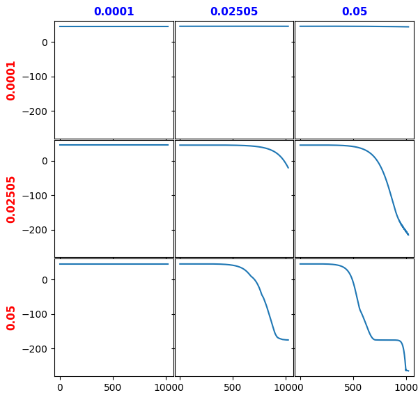
Figure 3: Evolution of the entropy for each of the learning rate configurations showing that the impact of picking the incorrect learning rate for the data and/or centroids lead to a collapse of the samples.

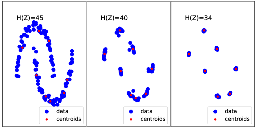
Figure 4: Evolution of GMM training when enforcing a one-to-one mapping between the data and centroids akin to K-means i.e. using a small and fixed covariance matrix. We see that collapse does not occur. Left - In the presence of fixed input samples, we observe that there is no collapsing and that the entropy of the centers is high. Right - when we make the input samples trainable and optimize their location, all the points collapse into a single point, resulting in a sharp decrease in entropy.

Appendix I On Benefits of Information Maximization for Generalization

In this Appendix, we present the complete version of Theorem 2 along with its proof and additional discussions.

I.1 Additional Notation and details

We start to introduce additional notation and details. We use the notation of $x\in\mathcal{X}$ for an input and $y\in\mathcal{Y}\subseteq\mathbb{R}^{r}$ for an output. Define $p(y)={\mathbb{P}}(Y=y)$ to be the probability of getting label $y$ and ${\hat{p}}(y)=\frac{1}{n}\sum_{i=1}^{n}\mathbbm{1}\{y_{i}=y\}$ to be the empirical estimate of $p(y)$. Let $\zeta$ be an upper bound on the norm of the label as $\|y\|_{2}\leq\zeta$ for all $y\in\mathcal{Y}$. Define the minimum norm solution $W_{\bar{S}}$ of the unlabeled data as $W_{\bar{S}}=\mathop{\mathrm{minimize}}_{W^{\prime}}\|W^{\prime}\|_{F}$ s.t. $W^{\prime}\in\operatorname*{arg\,min}_{W}\frac{1}{m}\sum_{i=1}^{m}\|Wf_{\theta}(x^{+}_{i})-g^{*}(x^{+}_{i})\|^{2}$. Let $\kappa_{S}$ be a data-dependent upper bound on the per-sample Euclidian norm loss with the trained model as $\|W_{S}f_{\theta}(x)-y\|\leq\kappa_{S}$ for all $(x,y)\in\mathcal{X}\times\mathcal{Y}$. Similarly, let $\kappa_{{\bar{S}}}$ be a data-dependent upper bound on the per-sample Euclidian norm loss as $\|W_{{\bar{S}}}f_{\theta}(x)-y\|\leq\kappa_{{\bar{S}}}$ for all $(x,y)\in\mathcal{X}\times\mathcal{Y}$. Define the difference between $W_{S}$ and $W_{\bar{S}}$ by $c=\|W_{S}-W_{\bar{S}}\|_{2}$. Let $\mathcal{W}$ be a hypothesis space of $W$ such that $W_{\bar{S}}\in\mathcal{W}$. We denote by $\tilde{\mathcal{R}}_{m}(\mathcal{W}\circ\mathcal{F})=\frac{1}{\sqrt{m}}\mathbb{E}_{{\bar{S}},\xi}[\sup_{W\in\mathcal{W},f\in\mathcal{F}}\sum_{i=1}^{m}\xi_{i}\|g^{*}(x^{+}_{i})-Wf(x^{+}_{i})\|]$ the normalized Rademacher complexity of the set $\{x^{+}\mapsto\|g^{*}(x^{+})-Wf(x^{+})\|:W\in\mathcal{W},f\in\mathcal{F}\}$. we denote by $\kappa$ a upper bound on the per-sample Euclidian norm loss as $\|Wf(x)-y\|\leq\kappa$ for all $(x,y,W,f)\in\mathcal{X}\times\mathcal{Y}\times\mathcal{W}\times\mathcal{F}$.

We adopt the following data-generating process model that is used in the previous paper on analyzing contrastive learning (Saunshi et al., 2019; Ben-Ari and Shwartz-Ziv, 2018). For the labeled data, first, $y$ is drawn from the distritbuion $\rho$ on $\mathcal{Y}$, and then $x$ is drawn from the conditional distribution $\mathcal{D}_{y}$ conditioned on the label $y$. That is, we have the join distribution $\mathcal{D}(x,y)=\mathcal{D}_{y}(x)\rho(y)$ with $((x_{i},y_{i}))_{i=1}^{n}\sim\mathcal{D}^{n}$. For the unlabeled data, first, each of the unknown labels $y^{+}$ and $y^{-}$ is drawn from the distritbuion $\rho$, and then each of the positive examples $x^{+}$ and $x^{++}$ is drawn from the conditional distribution $\mathcal{D}_{y^{+}}$ while the negative example $x^{-}$ is drawn from the $\mathcal{D}_{y^{-}}$. Unlike the analysis of contrastive learning, we do not require the negative samples. Let $\tau_{{\bar{S}}}$ be a data-dependent upper bound on the invariance loss with the trained representation as $\|f_{\theta}({\bar{x}})-f_{\theta}(x)\|\leq\tau_{{\bar{S}}}$ for all $({\bar{x}},x)\sim\mathcal{D}_{y}^{2}$ and $y\in\mathcal{Y}$. Let $\tau$ be a data-independent upper bound on the invariance loss with the trained representation as$\|f({\bar{x}})-f(x)\|\leq\tau$ for all $({\bar{x}},x)\sim\mathcal{D}_{y}^{2}$, $y\in\mathcal{Y}$, and $f\in\mathcal{F}$. For the simplicity, we assume that there exists a function $g^{*}$ such that $y=g^{*}(x)\in\mathbb{R}^{r}$ for all $(x,y)\in\mathcal{X}\times\mathcal{Y}$. Discarding this assumption adds the average of label noises to the final result, which goes to zero as the sample sizes $n$ and $m$ increase, assuming that the mean of the label noise is zero.

References

- Achille and Soatto (2018) Alessandro Achille and Stefano Soatto. Information dropout: Learning optimal representations through noisy computation. IEEE transactions on pattern analysis and machine intelligence, 40(12):2897–2905, 2018.
- Ahmed and Gokhale (1989) N.A. Ahmed and D.V. Gokhale. Entropy expressions and their estimators for multivariate distributions. IEEE Transactions on Information Theory, 35(3):688–692, 1989. doi: 10.1109/18.30996.
- Alemi et al. (2016) Alexander A Alemi, Ian Fischer, Joshua V Dillon, and Kevin Murphy. Deep variational information bottleneck. arXiv preprint arXiv:1612.00410, 2016.
- Arora et al. (2019) Sanjeev Arora, Hrishikesh Khandeparkar, Mikhail Khodak, Orestis Plevrakis, and Nikunj Saunshi. A theoretical analysis of contrastive unsupervised representation learning. arXiv preprint arXiv:1902.09229, 2019.
- Bachman et al. (2019) Philip Bachman, R Devon Hjelm, and William Buchwalter. Learning representations by maximizing mutual information across views. Advances in neural information processing systems, 32, 2019.
- Balestriero and Baraniuk (2018) Randall Balestriero and Richard Baraniuk. A spline theory of deep networks. In Proc. ICML, volume 80, pages 374–383, Jul. 2018.
- Balestriero and LeCun (2022) Randall Balestriero and Yann LeCun. Contrastive and non-contrastive self-supervised learning recover global and local spectral embedding methods, 2022. URL https://arxiv.org/abs/2205.11508.
- Bardes et al. (2021) Adrien Bardes, Jean Ponce, and Yann LeCun. Vicreg: Variance-invariance-covariance regularization for self-supervised learning. arXiv preprint arXiv:2105.04906, 2021.
- Bartlett and Mendelson (2002) Peter L Bartlett and Shahar Mendelson. Rademacher and gaussian complexities: Risk bounds and structural results. Journal of Machine Learning Research, 3(Nov):463–482, 2002.
- Bartlett et al. (2017) Peter L Bartlett, Dylan J Foster, and Matus J Telgarsky. Spectrally-normalized margin bounds for neural networks. Advances in neural information processing systems, 30, 2017.
- Belghazi et al. (2018) Mohamed Ishmael Belghazi, Aristide Baratin, Sai Rajeswar, Sherjil Ozair, Yoshua Bengio, Aaron Courville, and R Devon Hjelm. Mine: mutual information neural estimation. arXiv preprint arXiv:1801.04062, 2018.
- Ben-Ari and Shwartz-Ziv (2018) Itamar Ben-Ari and Ravid Shwartz-Ziv. Attentioned convolutional lstm inpaintingnetwork for anomaly detection in videos. arXiv preprint arXiv:1811.10228, 2018.
- Brewer (2017) Brendon J Brewer. Computing entropies with nested sampling. Entropy, 19(8):422, 2017.
- Caron et al. (2020) Mathilde Caron, Ishan Misra, Julien Mairal, Priya Goyal, Piotr Bojanowski, and Armand Joulin. Unsupervised learning of visual features by contrasting cluster assignments. Advances in Neural Information Processing Systems, 33:9912–9924, 2020.
- Caron et al. (2021) Mathilde Caron, Hugo Touvron, Ishan Misra, Hervé Jégou, Julien Mairal, Piotr Bojanowski, and Armand Joulin. Emerging properties in self-supervised vision transformers. In Proceedings of the IEEE/CVF International Conference on Computer Vision, pages 9650–9660, 2021.
- Chen et al. (2020) Ting Chen, Simon Kornblith, Mohammad Norouzi, and Geoffrey Hinton. A simple framework for contrastive learning of visual representations. In International conference on machine learning, pages 1597–1607. PMLR, 2020.
- Chen and He (2021) Xinlei Chen and Kaiming He. Exploring simple siamese representation learning. In Proceedings of the IEEE/CVF Conference on Computer Vision and Pattern Recognition, pages 15750–15758, 2021.
- Cheney and Light (2009) Elliott Ward Cheney and William Allan Light. A course in approximation theory, volume 101. American Mathematical Soc., 2009.
- D’Agostino (1971) Ralph B. D’Agostino. An omnibus test of normality for moderate and large size samples. Biometrika, 58(2):341–348, 1971. ISSN 00063444. URL http://www.jstor.org/stable/2334522.
- Dang et al. (2018) Zheng Dang, Kwang Moo Yi, Yinlin Hu, Fei Wang, Pascal Fua, and Mathieu Salzmann. Eigendecomposition-free training of deep networks with zero eigenvalue-based losses. In Proceedings of the European Conference on Computer Vision (ECCV), pages 768–783, 2018.
- Dubois et al. (2021) Yann Dubois, Benjamin Bloem-Reddy, Karen Ullrich, and Chris J Maddison. Lossy compression for lossless prediction. Advances in Neural Information Processing Systems, 34, 2021.
- Egerstedt and Martin (2009) Magnus Egerstedt and Clyde Martin. Control theoretic splines: optimal control, statistics, and path planning. Princeton University Press, 2009.
- Fantuzzi et al. (2002) Cesare Fantuzzi, Silvio Simani, Sergio Beghelli, and Riccardo Rovatti. Identification of piecewise affine models in noisy environment. International Journal of Control, 75(18):1472–1485, 2002.
- Federici et al. (2019) Marco Federici, Anjan Dutta, Patrick Forré, Nate Kushman, and Zeynep Akata. Learning robust representations via multi-view information bottleneck. In International Conference on Learning Representations, 2019.
- Federici et al. (2020) Marco Federici, Anjan Dutta, Patrick Forré, Nate Kushman, and Zeynep Akata. Learning robust representations via multi-view information bottleneck. arXiv preprint arXiv:2002.07017, 2020.
- Fefferman et al. (2016) Charles Fefferman, Sanjoy Mitter, and Hariharan Narayanan. Testing the manifold hypothesis. Journal of the American Mathematical Society, 29(4):983–1049, 2016.
- Giles (2008) Mike B. Giles. Collected matrix derivative results for forward and reverse mode algorithmic differentiation. In Christian H. Bischof, H. Martin Bücker, Paul Hovland, Uwe Naumann, and Jean Utke, editors, Advances in Automatic Differentiation, pages 35–44, Berlin, Heidelberg, 2008. Springer Berlin Heidelberg.
- Goldfeld et al. (2018) Z. Goldfeld, E. van den Berg, K. Greenewald, I. Melnyk, N. Nguyen, B. Kingsbury, and Y. Polyanskiy. Estimating Information Flow in Neural Networks. ArXiv e-prints, 2018.
- Golowich et al. (2018) Noah Golowich, Alexander Rakhlin, and Ohad Shamir. Size-independent sample complexity of neural networks. In Conference On Learning Theory, pages 297–299. PMLR, 2018.
- Goodfellow et al. (2016) I. Goodfellow, Y. Bengio, and A. Courville. Deep Learning, volume 1. MIT Press, 2016.
- Grill et al. (2020) Jean-Bastien Grill, Florian Strub, Florent Altché, Corentin Tallec, Pierre Richemond, Elena Buchatskaya, Carl Doersch, Bernardo Avila Pires, Zhaohan Guo, Mohammad Gheshlaghi Azar, et al. Bootstrap your own latent-a new approach to self-supervised learning. Advances in neural information processing systems, 33:21271–21284, 2020.
- Gunasekar et al. (2017) Suriya Gunasekar, Blake E Woodworth, Srinadh Bhojanapalli, Behnam Neyshabur, and Nati Srebro. Implicit regularization in matrix factorization. In Advances in Neural Information Processing Systems, pages 6151–6159, 2017.
- Gunasekar et al. (2018) Suriya Gunasekar, Jason D Lee, Daniel Soudry, and Nati Srebro. Implicit bias of gradient descent on linear convolutional networks. In Advances in Neural Information Processing Systems, pages 9461–9471, 2018.
- He et al. (2016) Kaiming He, Xiangyu Zhang, Shaoqing Ren, and Jian Sun. Deep residual learning for image recognition. In Proceedings of the IEEE Conference on Computer Vision and Pattern Recognition, pages 770–778, 2016.
- He et al. (2020) Kaiming He, Haoqi Fan, Yuxin Wu, Saining Xie, and Ross Girshick. Momentum contrast for unsupervised visual representation learning. In Proceedings of the IEEE/CVF conference on computer vision and pattern recognition, pages 9729–9738, 2020.
- Hjelm et al. (2018) R Devon Hjelm, Alex Fedorov, Samuel Lavoie-Marchildon, Karan Grewal, Phil Bachman, Adam Trischler, and Yoshua Bengio. Learning deep representations by mutual information estimation and maximization. arXiv preprint arXiv:1808.06670, 2018.
- Huber et al. (2008) Marco Huber, Tim Bailey, Hugh Durrant-Whyte, and Uwe Hanebeck. On entropy approximation for gaussian mixture random vectors. In IEEE International Conference on Multisensor Fusion and Integration for Intelligent Systems, pages 181 – 188, 09 2008. doi: 10.1109/MFI.2008.4648062.
- Ionescu et al. (2015) Catalin Ionescu, Orestis Vantzos, and Cristian Sminchisescu. Matrix backpropagation for deep networks with structured layers. In 2015 IEEE International Conference on Computer Vision (ICCV), pages 2965–2973, 2015. doi: 10.1109/ICCV.2015.339.
- Kahana and Hoshen (2022) Jonathan Kahana and Yedid Hoshen. A contrastive objective for learning disentangled representations. arXiv preprint arXiv:2203.11284, 2022.
- Kawaguchi et al. (2018) Kenji Kawaguchi, Leslie Pack Kaelbling, and Yoshua Bengio. Generalization in deep learning. MIT-CSAIL-TR-2018-014, Massachusetts Institute of Technology, 2018.
- Kawaguchi et al. (2022) Kenji Kawaguchi, Zhun Deng, Kyle Luh, and Jiaoyang Huang. Robustness Implies Generalization via Data-Dependent Generalization Bounds. In International Conference on Machine Learning (ICML), 2022.
- Kolchinsky and Tracey (2017) Artemy Kolchinsky and Brendan D Tracey. Estimating mixture entropy with pairwise distances. Entropy, 19(7):361, 2017.
- Krizhevsky (2009) Alex Krizhevsky. Learning multiple layers of features from tiny images. Technical report, 2009.
- Krizhevsky et al. (2009) Alex Krizhevsky, Geoffrey Hinton, et al. Learning multiple layers of features from tiny images. 2009.
- Lee et al. (2021a) Jason D Lee, Qi Lei, Nikunj Saunshi, and Jiacheng Zhuo. Predicting what you already know helps: Provable self-supervised learning. Advances in Neural Information Processing Systems, 34, 2021a.
- Lee et al. (2021b) Kuang-Huei Lee, Anurag Arnab, Sergio Guadarrama, John Canny, and Ian Fischer. Compressive visual representations. Advances in Neural Information Processing Systems, 34, 2021b.
- Linsker (1988) Ralph Linsker. Self-organization in a perceptual network. Computer, 21(3):105–117, 1988.
- Martinez et al. (2021) Julieta Martinez, Jashan Shewakramani, Ting Wei Liu, Ioan Andrei Bârsan, Wenyuan Zeng, and Raquel Urtasun. Permute, quantize, and fine-tune: Efficient compression of neural networks. In Proceedings of the IEEE/CVF Conference on Computer Vision and Pattern Recognition, pages 15699–15708, 2021.
- Misra and Maaten (2020) Ishan Misra and Laurens van der Maaten. Self-supervised learning of pretext-invariant representations. In Proceedings of the IEEE/CVF Conference on Computer Vision and Pattern Recognition, pages 6707–6717, 2020.
- Misra et al. (2005) Neeraj Misra, Harshinder Singh, and Eugene Demchuk. Estimation of the entropy of a multivariate normal distribution. Journal of Multivariate Analysis, 92(2):324–342, 2005. ISSN 0047-259X. doi: https://doi.org/10.1016/j.jmva.2003.10.003.
- Mohri et al. (2012) Mehryar Mohri, Afshin Rostamizadeh, and Ameet Talwalkar. Foundations of machine learning. MIT press, 2012.
- Montufar et al. (2014) Guido F Montufar, Razvan Pascanu, Kyunghyun Cho, and Yoshua Bengio. On the number of linear regions of deep neural networks. In Proc. NeurIPS, pages 2924–2932, 2014.
- Nowozin et al. (2016) Sebastian Nowozin, Botond Cseke, and Ryota Tomioka. f-gan: Training generative neural samplers using variational divergence minimization. In Advances in Neural Information Processing systems, pages 271–279, 2016.
- Oord et al. (2018) Aaron van den Oord, Yazhe Li, and Oriol Vinyals. Representation learning with contrastive predictive coding. arXiv preprint arXiv:1807.03748, 2018.
- Piran et al. (2020) Zoe Piran, Ravid Shwartz-Ziv, and Naftali Tishby. The dual information bottleneck. arXiv preprint arXiv:2006.04641, 2020.
- Saunshi et al. (2019) Nikunj Saunshi, Orestis Plevrakis, Sanjeev Arora, Mikhail Khodak, and Hrishikesh Khandeparkar. A theoretical analysis of contrastive unsupervised representation learning. In International Conference on Machine Learning, pages 5628–5637. PMLR, 2019.
- Shalev-Shwartz and Ben-David (2014) Shai Shalev-Shwartz and Shai Ben-David. Understanding machine learning: From theory to algorithms. Cambridge university press, 2014.
- Shwartz-Ziv (2022) Ravid Shwartz-Ziv. Information flow in deep neural networks. arXiv preprint arXiv:2202.06749, 2022.
- Shwartz-Ziv and Alemi (2020) Ravid Shwartz-Ziv and Alexander A Alemi. Information in infinite ensembles of infinitely-wide neural networks. In Symposium on Advances in Approximate Bayesian Inference, pages 1–17. PMLR, 2020.
- Shwartz-Ziv and LeCun (2023) Ravid Shwartz-Ziv and Yann LeCun. To Compress or Not to Compress - Self-Supervised Learning and Information Theory - A Review. 2023.
- Shwartz-Ziv and Tishby (2017a) Ravid Shwartz-Ziv and Naftali Tishby. Compression of deep neural networks via information, (2017). arXiv preprint arXiv:1703.00810, 2017a.
- Shwartz-Ziv and Tishby (2017b) Ravid Shwartz-Ziv and Naftali Tishby. Opening the black box of deep neural networks via information. arXiv preprint arXiv:1703.00810, 2017b.
- Shwartz-Ziv et al. (2018) Ravid Shwartz-Ziv, Amichai Painsky, and Naftali Tishby. Representation compression and generalization in deep neural networks, 2018.
- Shwartz-Ziv et al. (2022) Ravid Shwartz-Ziv, Micah Goldblum, Hossein Souri, Sanyam Kapoor, Chen Zhu, Yann LeCun, and Andrew Gordon Wilson. Pre-train your loss: Easy bayesian transfer learning with informative priors. arXiv preprint arXiv:2205.10279, 2022.
- Shwartz-Ziv et al. (2023) Ravid Shwartz-Ziv, Randall Balestriero, Kenji Kawaguchi, and Yann LeCun. What do we maximize in self-supervised learning and why does generalization emerge?, 2023. URL https://openreview.net/forum?id=tuE-MnjN7DV.
- Soudry et al. (2018) Daniel Soudry, Elad Hoffer, Mor Shpigel Nacson, Suriya Gunasekar, and Nathan Srebro. The implicit bias of gradient descent on separable data. The Journal of Machine Learning Research, 19(1):2822–2878, 2018.
- Steinke and Zakynthinou (2020) Thomas Steinke and Lydia Zakynthinou. Reasoning about generalization via conditional mutual information. In Conference on Learning Theory, pages 3437–3452. PMLR, 2020.
- Wang et al. (2022) Haoqing Wang, Xun Guo, Zhi-Hong Deng, and Yan Lu. Rethinking minimal sufficient representation in contrastive learning. In Proceedings of the IEEE/CVF Conference on Computer Vision and Pattern Recognition, pages 16041–16050, 2022.
- Wang and Isola (2020) Tongzhou Wang and Phillip Isola. Understanding contrastive representation learning through alignment and uniformity on the hypersphere. In International Conference on Machine Learning, pages 9929–9939. PMLR, 2020.
- Xu and Raginsky (2017) Aolin Xu and Maxim Raginsky. Information-theoretic analysis of generalization capability of learning algorithms. Advances in Neural Information Processing Systems, 30, 2017.
- Zbontar et al. (2021) Jure Zbontar, Li Jing, Ishan Misra, Yann LeCun, and Stéphane Deny. Barlow twins: Self-supervised learning via redundancy reduction. In International Conference on Machine Learning, pages 12310–12320. PMLR, 2021.
- Zhouyin and Liu (2021) Zhanghao Zhouyin and Ding Liu. Understanding neural networks with logarithm determinant entropy estimator. arXiv preprint arXiv:2105.03705, 2021.
- Zimmermann et al. (2021) Roland S Zimmermann, Yash Sharma, Steffen Schneider, Matthias Bethge, and Wieland Brendel. Contrastive learning inverts the data generating process. In International Conference on Machine Learning, pages 12979–12990. PMLR, 2021.