Drastic magnetic-field-induced chiral current order and emergent current-bond-field interplay in kagome metal AV3Sb5 (A=Cs,Rb,K)
Abstract
In kagome metals, the chiral current order parameter with time-reversal-symmetry-breaking is the source of various exotic electronic states, while the method of controlling the current order and its interplay with the star-of-David bond order are still unsolved. Here, we reveal that tiny uniform orbital magnetization is induced by the chiral current order, and its magnitude is prominently enlarged under the presence of the bond order. Importantly, we derive the magnetic-field ()-induced Ginzburg-Landau (GL) free energy expression , which enables us to elucidate the field-induced current-bond phase transitions in kagome metals. The emergent current-bond- trilinear coupling term in the free energy, , naturally explains the characteristic magnetic field sensitive electronic states in kagome metals, such as the field-induced current order and the strong interplay between the bond and current orders. The GL coefficients of derived from the realistic multiorbital model are appropriate to explain various experiments. Furthermore, we present a natural explanation for the drastic strain-induced increment of the current order transition temperature reported by a recent experiment.
Introduction
Recent discovery of unconventional quantum phases in metals has led to a new trend of condensed matter physics. Exotic charge-density-wave orders and unconventional superconductivity in geometrically frustrated kagome metal AV3Sb5 (A=Cs,Rb,K) have been attracting increasing attention kagome-exp1 ; kagome-exp2 . The 22 (inverse) star-of-David order, which is presumably the triple- () bond order (BO), occurs at K at ambient pressure STM1 ; STM2 . The BO is the time-reversal-symmetry (TRS) preserving modulation in the hopping integral, . Thomale2013 ; SMFRG ; Thomale2021 ; Neupert2021 ; Balents2021 ; Nandkishore ; Tazai-kagome . Below , nodeless superconductivity occurs for A=Cs Roppongi ; SC2 , which is naturally explained based on the BO fluctuation mechanism proposed in Ref. Tazai-kagome .
In kagome metals, unusual TRS breaking (TRSB) phase without long-range spin orders has been reported by -SR muSR3-Cs ; muSR2-K ; muSR4-Cs ; muSR5-Rb , Kerr rotation birefringence-kagome ; Yonezawa , field-tuned chiral transport eMChA measurements and STM studies under magnetic field STM1 ; eMChA . The transition temperature is still under debate. Although it is close to in many experiments, the TRSB order parameter is strongly magnified at K for A=Cs eMChA ; muSR3-Cs ; muSR4-Cs and K for A=Rb muSR5-Rb . Recently, magnetic torque measurement reveals the nematic order with TRSB at K Asaba , while no TRSB was reported by recent Kerr rotation study Kapitulnik . A natural candidate is the correlation driven TRSB hopping integral modulation: . This order accompanies topological charge-current Haldane that gives the giant anomalous Hall effect (AHE) AHE1 ; AHE2 .
Theoretically, the BO and the current order emerge in the presence of sizable off-site electron correlations in Fe-based and cuprate superconductors Onari-SCVC ; Yamakawa-FeSe ; Onari-TBG ; Tsuchiizu1 ; Tsuchiizu4 ; Chubukov-PRX2016 ; Fernandes-rev2018 ; Kontani-AdvPhys ; Davis-rev2013 and in kagome metals Thomale2021 ; Neupert2021 ; Balents2021 ; Tazai-kagome ; Tazai-kagome2 ; PDW-kagome ; Fernandes-GL ; Thomale-GL ; Nat-g-ology . Notably, strong off-site interaction (due to the off-site Coulomb repulsion or the BO fluctuations) gives rise to the charge current order Neupert2021 ; Balents2021 ; Nandkishore ; Tazai-kagome2 . Based on the GL free-energy analysis, interesting bond+current nematic () coexisting phases have been discussed in two-dimensional (2D) and three-dimensional (3D) models Balents2021 ; Tazai-kagome2 ; Fernandes-GL ; Thomale-GL ; Nat-g-ology . Experimentally, the nematic state is actually observed by the elastoresistance elastoresistance-kagome , the scanning birefringence birefringence-kagome , and the STM STM2 measurements.
In kagome metals, outer magnetic field drastically modifies the electronic states. The chirality of the charge-current is aligned under very tiny Tesla according to the measurements of AHE AHE1 ; AHE2 and field-tuned chiral transport eMChA . In addition, the amplitude of the loop current is strongly magnified by applying small muSR4-Cs ; muSR2-K ; muSR5-Rb . Very recent transport measurement of highly symmetric fabricated CsV3Sb5 micro sample Moll-hz reveals that current-order state is drastically enlarged by the small . These drastic -dependences are the hallmarks of the TRSB state, and it is important to understand the coupling between the current order, chirality and the magnetic field in kagome metals.

In this paper, we reveal that the loop-current order parameters accompany tiny orbital magnetization, , and its magnitude is drastically enlarged under the presence of the bond order. Importantly, we derive the -induced Ginzburg-Landau (GL) free energy expression , which is useful to study nontrivial phase transitions under the magnetic field. The emergent current-bond- trilinear coupling term in not only explains the origin of novel field-induced chiral symmetry breaking muSR4-Cs ; muSR2-K ; muSR5-Rb but also provides useful hints to control the charge current in kagome metals. In addition, the “strain-induced increment of reported in Ref. Moll-hz is naturally understood.
In the present study of , we mainly focus on the current order in the -orbital (in -representation) of V ion, which has been intensively studied previously Thomale2021 ; Neupert2021 ; Balents2021 ; Nandkishore ; Tazai-kagome2 . However, other -orbitals (especially -, -, -orbitals) also form the large Fermi surfaces (FSs) with the van-Hove singularity (vHS) points near the Fermi level. The impact of these non- orbitals on the current order has also been studied in Refs. Fernandes-GL ; Nat-g-ology . The present field-induced GL theory does not depend on the -orbital character of the current order parameter. We calculate the GL coefficients () for various -orbital current order states based on the first-principles kagome metal models. For a fixed order parameter, is large when the FS reconstruction due to the current order parameters occurs near the vHS points.
Model Hamiltonian with current and bond orders
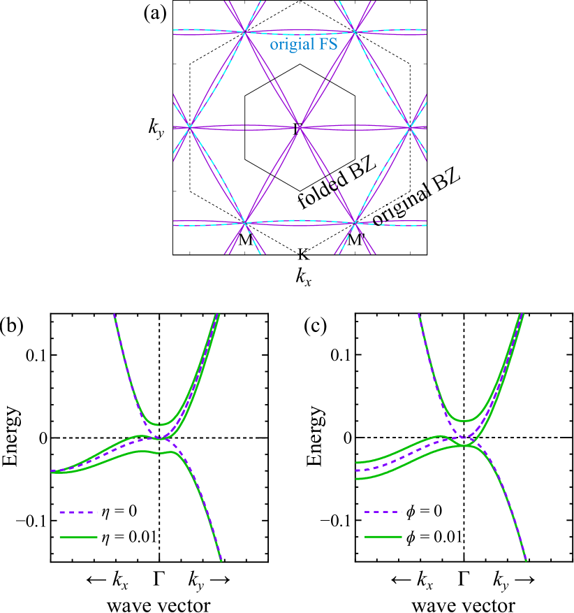
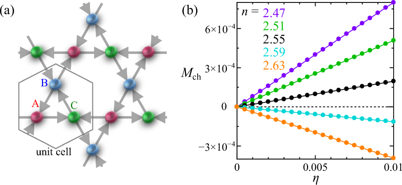
Here, we study the kagome-lattice tight-binding model with (or ) orbitals shown in Fig. 1 (a). Each unit-cell is composed of three sublattices A, B, C. We set the nearest-neighbor hopping integral . In addition, we introduce the nearest intra-sublattice hopping shown in Fig. 1 (a) to avoid the perfect nesting. (Hereafter, the unit of the energy is eV.) The FS at the vHS filling, per 3-site unit cell, is shown in Fig. 1 (b). Then, the FS lies on the three vHS points (, , ), each of which is composed of a single sublattice A, B, or C. This simple three-orbital model well captures the main pure-type FS in kagome metals STM1 ; ARPES-VHS ; ARPES-band ; ARPES-Lifshitz ; Sato-ARPES .
The bond/current order is the modulation of the hopping integral between and atmos due to the electron correlation, . Theoretically, it is the symmetry breaking in the self-energy, and it is derived from the density-wave (DW) equation Tazai-kagome ; Tazai-kagome2 . The wavevectors of the bond and current orders correspond to the inter-sublattice nesting vectors () in Fig. 1 (b) according to previous theoretical studies Thomale2021 ; Neupert2021 ; Balents2021 ; Tazai-kagome ; Tazai-kagome2 ; PDW-kagome . The triple () current order between the nearest atoms is depicted in Fig. 1 (c). The form factor (=normalized ) with , , is for belongs to the sites in Fig. 1 (c), and for . Odd parity relation holds. Other form factors with and , and , are also derived from Fig. 1 (c). Using , the current order is
| (1) |
where is the set of current order parameters with the wavevector . Also, the BO is given as
| (2) |
where is the set of BO parameters with the wavevector , and is the even-parity form factor for the BO shown in Fig. 1 (a). For example, for belongs to [].
The unit cell under the bond/current order is magnified by times. Thus, we analyze the electronic states with the current order based on the -site kagome lattice model. The Hamiltonian with the bond+current order is , where and is the Fourier transform of the hopping integral . Here, is the hopping integral of the original model, and is the hopping integral due to the bond (current) order in Eq. [2] (Eq. [1]).
Uniform orbital magnetization
The TRS is broken in the presence of the current order . In this case, the uniform orbital magnetization may appear due to the finite Berry curvature as pointed out in Ref. Balents2021 . per V atom in the unit of Bohr magneton (= free electron mass) is given as Morb-paper1 ; Morb-paper2
| (3) | |||||
| (5) | |||||
where is -th eigenenergy of -site kagome lattice model in the folded BZ. is Fermi distribution function, is the site number of unit cell, is the -mesh number, and . is the unit length in the numerical study, and we set ( nm in kagome metals). eV when nm.
At zero temperature, Eq. [3] is rewritten as
| (6) | |||||
where is the Fermi distribution function at . Considering the factor with , originates from the “vertical particle-hole (p-h) excitation”, from to , at the same in the folded BZ.
The folded FS () and bandstructure in the folded Brillouin zone (BZ) at are shown in Figs. S1 (a)-(c) in the SI A SM . Here, all vHS points A, B, C in the original BZ in Fig. 1 (b) move to point, and they will hybridize each other due to the current and/or BO parameter. When , prominent band hybridization occurs near the point, as understood in Fig. S1 (a). Then, the bonding (antibonding) band energy at point is below (above) the Fermi level, as shown in Fig. S1 (b). Because of the factor in Eq. [6], becomes large when .
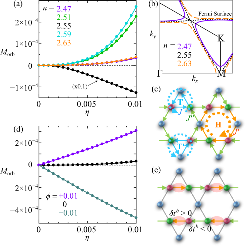
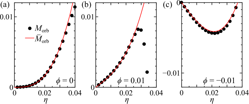
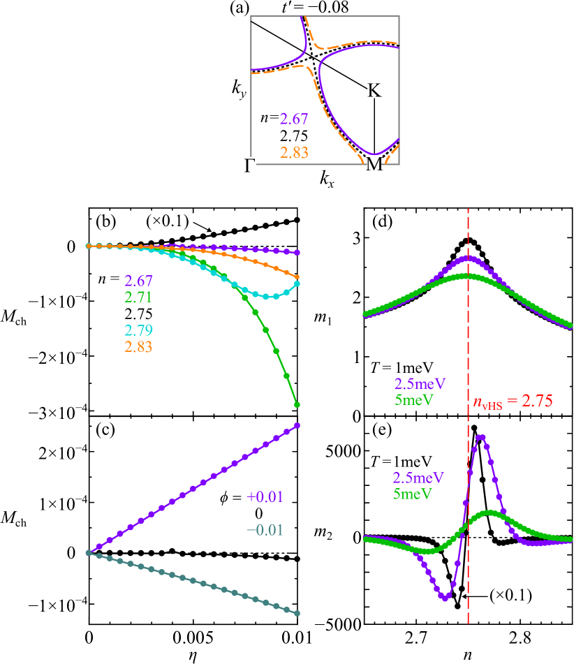
Here, we calculate [] near the vHS filling at meV, in the case of eV. Figure 2 (a) represents the obtained under the current order for . (The FS without the current order is shown in Fig. 2 (b).) We obtain the relation , and it becomes large when the filling is close to . Therefore, the current order state is a weak-ferromagnetic (or ferrimagnetic) state. Because the additional free energy under the magnetic field per 3-site unit cell is
| (7) |
the chirality of the current order is aligned under tiny . In other words, the current order is stabilized under . In contrast, for and current orders. corresponds to Tesla.
Here, we present a symmetry argument to understand induced by the current order. Both and current orders are invariant under the time-reversal and the translational operations successively. Therefore, due to the TRS in the bulk state. In contrast, is nonzero in the current order because this state breaks the TRS in the bulk state Balents2021 . To find an intuitive reason, we calculated the charge-current along the nearest bonds in the state using the method in Refs. Tazai-cLC ; Kontani-AdvPhys , and found that is bond-dependent in spite of the same order parameter . The obtained relation shown in Fig. 2 (c) indicates that becomes finite because the magnetic fluxes through triangles and hexagons do not cancel perfectly.
For general order parameter , we verified the relation up to the third-order. In fact, based on the perturbation theory with respect to Eq. [1]; (). is expanded as with because is an odd function of . In addition, can be nonzero only when (modulo original reciprocal vectors), because we study the nonlinear response of the uniform () magnetization due to the potential with wavevector in the original unit cell. (See the SI B for a more detailed explanation SM .) In Fig. 2 (a), originates from the third-order term , which is allowed because of the momentum conservation .
Next stage, we calculate under the coexistence of the current order and the bond order . Figure 2 (d) represents at as a function of , for and meV. Interesting relation is obtained when . Then, the field-induced contains a non-analytic -linear term that always produces . This fact causes significant field-induced change in the phase diagram, as we will explain in the SI C SM .
To understand the -linear term in Fig. 2 (d), we expand with respect to the current order and bond order . Its Taylor expansion is with and (modulo original reciprocal vectors). The -linear term in Fig. 2 (c) mainly originates from the second-order term in addition to the third-order term . In fact, the current + BO state shown in Fig. 2 (e) violates the TRS in the bulk state.
Field-induced GL free energy expression
From the above discussions, we obtain the following convenient expression of the orbital magnetization and the “field-induced GL free energy formula” up to the third-order:
| (8) | |||||
| (9) |
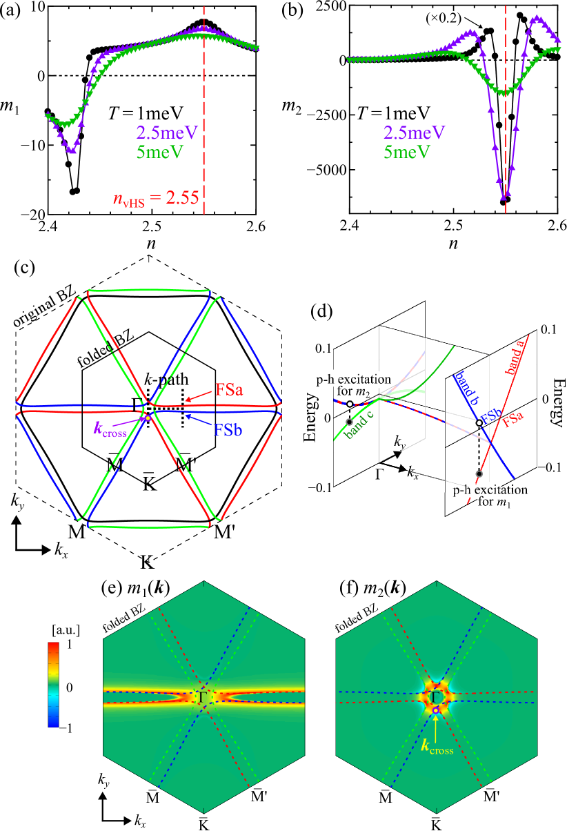
which enables us to elucidate the field-induced bond+current phase transitions in kagome metals. Figures 3 (a) and (b) show the coefficients and derived from Eq. [3] numerically, respectively. Interestingly, and become large for .
In the SI D SM , we show that in Eq. [8] well reproduces the original when . The expression of is also justified based on the first principles model for in the SI D SM .
To understand the -dependences of and , we discuss the folded FS and bandstructure given in Figs. 3 (c) and (d), respectively, for . Here, band [, and ] originates from the bandstructure around vHS-A [B,C] in Fig. 1 (b). As shown in Fig. 3 (d), band and band degenerate along -axis and -axis. Hereafter, we set .
First, we consider the origin of , which is caused by the band-folding induced by and , both of which convey the wavevector . Therefore, is induced by the “vertical p-h excitation between band and band ” in Fig. 3 (d) in the folded BZ. (Band gives no contribution for .) To verify this consideration, we examine the function in Eq. [5]. Figure 1 (e) shows the obtained . (Note that .) It is verified that large originates from the FS and FS near the -M line in Fig. 3 (c). This mechanism occurs for both and , so takes large value for a wide range of . Note that in Fig. 3 (a) changes its sign at , when and in Fig.1 (b) touch in the folded BZ.
Next, we consider the origin of , which is caused by the band-foldings caused by (at ), (at ) and (at ). This situation allows the “vertical p-h excitation between band and band ” in Fig. 3 (d), which is significant because the band splitting between and is very small. This process gives huge at obtained in Fig. 3 (b). Figure 3 (f) shows the obtained . (Note that .) The large originates from the six band-crossing points () near the point, due to the vertical p-h excitation among three bands , , .
To summarize, large and are caused by the FS crossing near the vHS points and the M-M’ line for . Therefore, the field-induced free energy should be significant in real kagome metals. In the SI B SM , we verify that the relation holds very well. This relation originates from the relation or when both order parameters are composed of only the nearest bonds.
We verified in the SI E SM that the magnitudes of and at is comparable to those in Fig. 3. When in Fig. 3 (b), the obtained takes a large value because the p-h asymmetry around is significant. When in Fig. S6 (e), in contrast, is small and tends to be an odd function of because of the approximate p-h symmetry and the factor in Eq. [6]. (The numerical results of in the 30-orbital model in Figs. 5 (g)-(h) are closer to the results at near the vHS filling.)
Below, we derive the order parameters under by minimizing the GL free energy , where is the free energy at Balents2021 ; Tazai-kagome2 :
| (10) | |||
| (11) |
and contains the current-bond cross terms proportional to and :
| (12) |
Here, , where is the current-order (BO) transition temperature without other orders. Theoretically, , where is the density-of-states () and is the DW equation eigenvalue of the current order (bond order) Tazai-LW . at , while (i.e., ) in the absence of interaction. According to Ref. Tazai-LW , for the nematic BO in FeSe, while the corresponding value for BCS superconductors is .
To discuss the phase diagram qualitatively, we set , , both of which are moderate compared with the values in Fig. 3. We also put by seeing the numerical results in the SI F SM and set . Then, both current and bond orders become states because of the relations and . A more detailed explanation for the GL parameters is presented in the SI F SM .
-effect on current order state
In this section, we demonstrate that the current order state is drastically modified by . Figure 4 (a) shows the obtained current order with , when in the absence of BO (). Here, we set . Because of the -term by , current order with negative is stabilized in the presence of . In addition, the field-induced first-order transition occurs at , where is quite small.
Next, we demonstrate the -induced current order state above inside the BO state. Under the BO phase , the 2nd order GL coefficient in Eq. [11] is renormalized as due to the , terms. It is given as , where and as we explain in the SI F SM . The smallness of is favorable for the -induced current order. In this subsection, we simply denote and as and , respectively.
First, we drop the 3rd order GL terms () to concentrate on the field-induced novel phenomena. Figure 4 (b) exhibits the current order with , in the presence of the BO phase below . For and , starts to emerge just below thanks to the -linear term , and therefore . When , is just a crossover temperature. To understand the role of the non-analytic term qualitatively, we analyze a simple GL free energy with a -linear term in the SI C SM : It is found that the field-induced current order under the BO is approximately given as
| (13) |
Thus, the field-induced is prominent when the system at is close to the current order state (i.e., ). The expression of in Eq. [13] is proportional to in contrast to Eq. (31) of Ref. Balents2021 .
A schematic picture for the field-induced current order is shown in Fig. 4 (c). In the BO phase , the field-induced above is proportional to to maximize . This coexisting state () has symmetry; see Ref. Tazai-kagome2 .
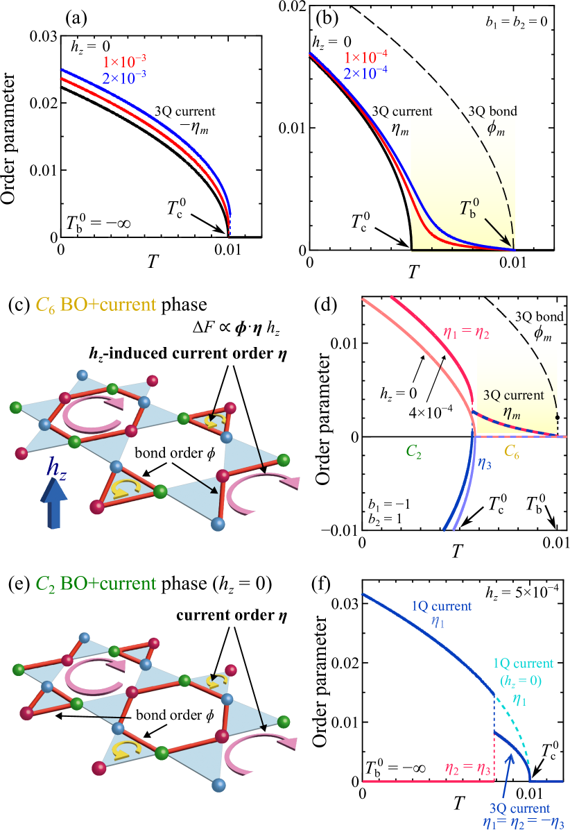
Next, we consider the effect of 3rd order GL terms in Fig. 4 (d), by setting . (The relation is general Tazai-kagome2 .) Due to the energy gain from the -term, 3Q BO appears at as the first order transition Balents2021 . At , the 3Q current order appears below to maximize the energy gain from the term (), as explained in Ref. Tazai-kagome2 . Just below (), is satisfied. (More generally, .) Figure 4 (e) depicts the “nematic” bond+current coexisting state below with and ; see Ref. Tazai-kagome2 for detail.
For in Fig. 4 (d), the field-induced current order start to emerge just below , similarly to Fig. 4 (b). The realized symmetry coexisting state above is shown in Fig. 4 (c). Below , the coexisting state changes to the nematic () bond+current state shown in Figure 4 (e). We stress that changes at . To summarize, the -induced coexisting state changes its symmetry from () to () with decreasing . The field-induced first-order phase transition occurs at .
-effect on current order state
In this scetion, we explain that the current order state is also drastically modified by . Here, we increase to (i.e., ) in the previous GL parameters. A clear evidence of the current order has been reported recently in Ref. Asaba . We set . Figure 4 (f) shows the obtained order parameters without BO () at . We obtain the field-induced -current order due to the -term, while it changes to order at . The field-induced first-order transitions reported in Ref. Asaba would originate from the current order at together with . In Fig. 4 (f), we set and . The obtained -induced current order is realized even when when .
In Fig. 4 (f), we set for simplicity. However, experimentally. In this case, as revealed in Ref. Balents2021 , the current order induces the finite BO even above via the term. This fact means that the current order is energetically favorable when . Therefore, -induced transition from to current order shown in Fig. 4 (f) can emerge even if for .
For reference, we studied the case of the intra-original-unit-cell current order () in kagome lattice in the SI G SM . In this case, is -linear even if the BO is absent.
Derivation of GL coefficients based on the first-priciples kagome metal model
In the next stage, we calculate the GL coefficients based on the first-principles tight-binding model for kagome metals. We reveal that and becomes large due to the “inter-orbital () mixture” even if the current order emerges only in the -orbital.
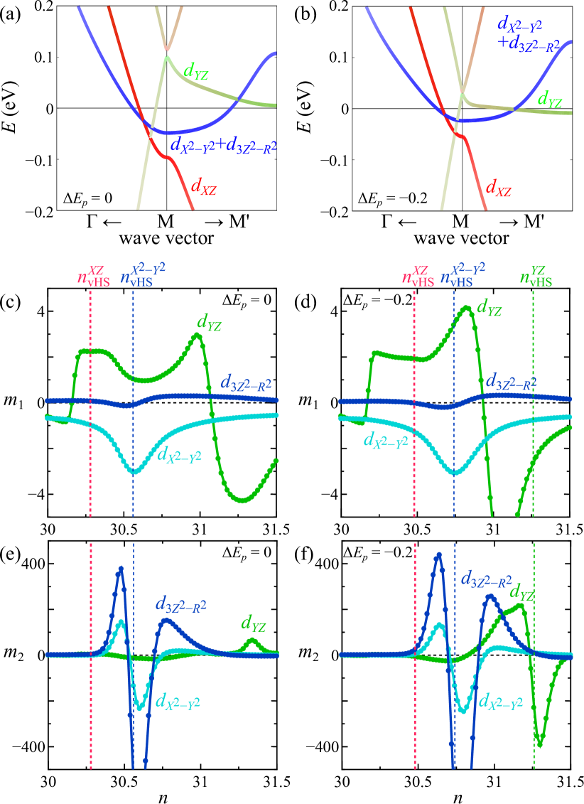
First, we derive 30-orbital (15 -orbital and 15 -orbitals) tight-binding model for CsV3Sb5 by using WIEN2k and Wannier90 softwares. Figure 5 (a) shows the FS of the obtained model in the plane. (Its bandstructure is shown in Fig. S9 (a).) The -orbital “pure-type” FS corresponds to the FS of the present three-orbital model. Its vHS energy is located at . Also, the -orbital forms the “mix-type” FS whose vHS energy is . In addition, both and orbitals form one pure-type band with the vHS energy .
Figure 5 (b) shows the FS with introducing the -orbital shift eV. Its bandstructure is shown in Fig. S9 (b). Here, the -orbital (mix-type) FS approaches the M point, and its vHS point shifts to the Fermi level, consistently with the ARPES measurement in Ref. ARPES-VHS . Figure 5 (c) shows the change in the FS topology due to the pure-mix hybridization in the model for . When , we obtain two hole-pockets that attach the M point. With increasing , it changes to the electron-like Dirac pockets at , composed of both and orbitals. At , large hole-like pure-type FS and large electron-like mix-type FS are formed. At , the mix-type FS lines on the M-M’ line. We will see that large and appear at , and .
Figure 5 (d) shows the obtained with the folded FSs. For both and , the pure-mix hybridization contributes to the large GL coefficient in the 30-orbital model. This mechanism is absent in the simple single orbital model.
We note that is reported in an ARPES study for pristine CsV3Sb5 in Ref. Sato-ARPES . In this case, both and become very large theoretically.
Now, we calculate and in by introducing the current and bond orders on the orbitals in the 30-orbital kagome lattice model given in Figs. 5 (a) () and (b) (). We derive the coefficients and defined as , where and are the -orbital order parameters projected on the pure-type band. (We set and with , which is the -weight on the pure-type band.)
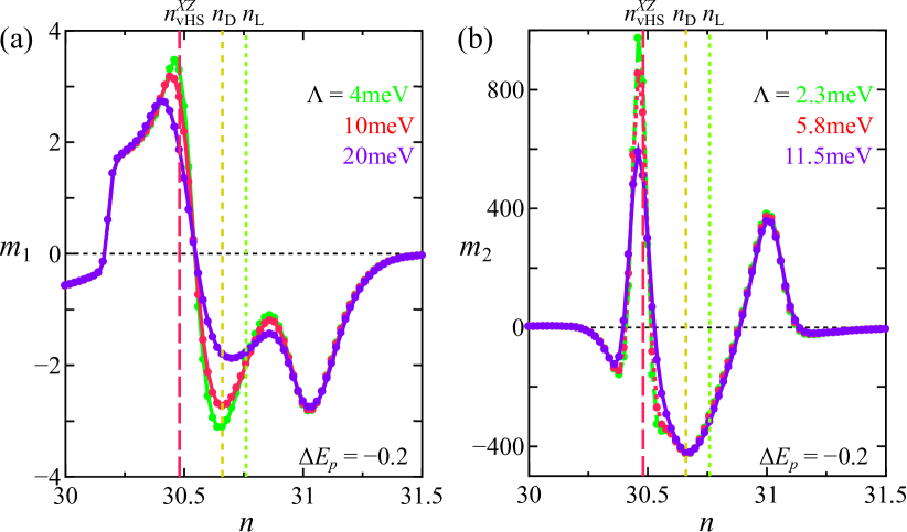
The obtained is shown in Figs. 5 (e) () and (f) (), as function of the electron filling . Here, is derived from the plane electronic structure. First, we discuss the case that corresponds to undoped CsV3Sb5. In both Figs. 5 (e) and (f), the obtained is very larger for . At , in Fig. 5 (e) is relatively small () accidentally, while its magnitude becomes large () in Fig. 5 (f), where the mix-type FS is closer to the M-M’ line. In fact, the mix-type FS contains finite -weight (%) owing to the inter-orbital mixture in kagome metal bandstructure. For this reason, the mix-type band can cause large even if the current order parameter occurs only in -orbital. Thus, the current-bond-field trillinear coupling due to term will cause the drastic field-induced chiral current order shown in Fig. 4 (b). This is the main result of this study.
The obtained is shown in Figs. 5 (g) () and (h) (), at and . The obtained is extremely larger for . At , becomes relatively small () in Fig. 5 (g). However, increases to in Fig. 5 (h) because the mix-type FS is closer to the M-M’ line. Thus, large can be realized by the mix-type band with finite -orbital weight even when . We stress that the relation is well satisfied; see the SI B SM .
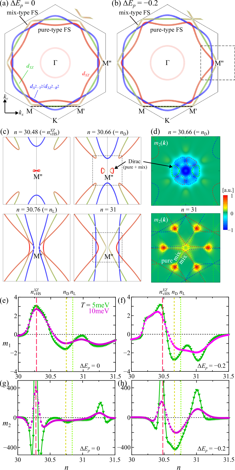
Next, we discuss the -dependences of and in more detail. In Figs. 5 (e)-(h), both coefficients take very large values at due to the hybridization between -orbital bands, as we explained in Fig. 3. With increasing , these coefficients exhibit drastic -dependences when the FS changes its topology due to the pure-mix hybridization. When , the electron-like Dirac pockets made of orbitals cause large and . and are also enlarged when the mix-band (with finite -weight) is close to the M-M’ line at in model [at in model].
To summarize, both and exhibit interesting sensitivity to the multiorbital character and the nesting condition of the bandstructure around M points. Unexpectedly, both -orbital (pure-type) band and -orbital (mix-type) band play important role for and even when the current order emerges only on the -orbital. When , the mix-type FS approaches the M point, consistently with the ARPES bandstructure ARPES-VHS . Then, we obtain large and at as shown in Figs. 5 (f) and (h). Thus, the -induced change in Fig. 4 can be obtained by changing the parameters slightly. (“Nearly commensurate” current order may appear in model, in which the nesting of the FS at is not perfect Tazai-kagome . The calculated will be larger by using the correct incommensurate nesting vector of model. ) In the SI H SM , we calculate the GL coefficients when the current and bond orders emerge on other -orbitals. It is found that large and are obtained in various cases. Thus, the present study is valid for various types of current order mechanisms, not restricted to Ref. Tazai-kagome2 .
Summary and Discussions
In summary, the chiral current order in kagome metal exhibits weak ferromagnetism, and its magnitude are enlarged in the bond order state. Importantly, we derived the -induced GL free energy expression in Eq. [9], which provides an important basis for future research in kagome metals. The emergent trilinear term in explains prominent field-induced chiral symmetry breaking in kagome metals. We revealed that becomes large when the vHS energy is close to the Fermi level because the prominent FS reconstruction occurs due to the current order parameters. Furthermore, the multi-orbital mixing in the bandstructure of real kagome metals makes larger for a wide filling range. The finding that sensitively depends on the multiorbital bandstructure in Fig. 5 provides a useful hint to control the charge current or to understand the difference between Cs-based and K-based compounds Moll-K . Interestingly, we obtain large when the current order parameter emerges in not only -orbital, but also other -orbitals. It is interesting to study for theoretically proposed exotic TRS breaking states, such as the inter-orbital exciton order Nat-g-ology and multipolar and toroidal magnetic orders Fernandes-GL .
Below, we discuss several important issues.
.1 Comparison with experiments: –induced current order
In Ref. Moll-hz , it was proposed that CsV3Sb5 is located at the quantum critical point of the current order () in the absence of the uniaxial strain. (As we discussed above, is renormalized to under the BO phase.) The field-induced (T) current order at K is naturally understood based on the GL free energy analysis with the current-bond- trillinear term. Figures 4 (b) and (d) corresponds to the experimental report in Ref. Moll-hz by considering that . In addition, the present GL theroy explains the field-induced enhancement of the local magnetic flux () observed by SR measurements in AV3Sb5 muSR4-Cs ; muSR2-K ; muSR5-Rb and field-tuned chiral transport study eMChA . Interestingly, the obtained sensitively depends on the multiorbital bandstructure and the filling in Fig. 5 (and Fig. S9). The present discovery provides a useful hint to control the charge current in kagome metals. The present finding will also be essential to understand the significant difference between Cs-based and K-based compounds reported in Ref. Moll-K . In addition, the discovery of CDW state in double-layer kagome metal ScV6Sn6 166-CDW has attracted increasing theoretical interest Thomale-GL ; Bernevig-166-exp ; Bernevig-166 . The TRS breaking state and its increment under discovered in ScV6Sn6 166-mSR may be understood by developing the present GL theory.
We note that the trilinear term in is also caused by the spin magnetization in the presence of spin-orbit interaction Fernandes-GL . Future quantitative calculations would be important.
.2 Comparison with experiments: Strain-induced current order
Reference Moll-hz also reports interesting prominent strain induced increment of . Under the uniaxial strain, the degeneracy of the current order transition temperature at (), , is lifted by the change in the 2nd order GL term as discussed in Ref. Moll-hz . Then, will be larger than the original . In the SI I SM , we find that additional significant contribution to the increment of originates from the strain induced change in the 4th order GL terms (). Here, the “BO-induced suppression of the current order by and GL terms is found to be drastically reduced by the strain. In fact, we find that is sensitive to the strain because the vHS energy is close to the Fermi level; see Fig. S10 in the SI I SM .
Below, we explain the discussion in the SI I SM . Considering the symmetry, we assume that the symmetry strain induces the shift of the vHS energy levels as . ( by is presented in the SI I SM .) Hereafter, we set . Under the BO phase , the 2nd order GL coefficient in Eq. [11] in the absence of the strain () is changed to
| (14) | |||||
where when . Here, we assume that is -independent because we study the strain-induced current order for . For finite , it is changed by as
| (15) | |||||
where are -linear. Here, . and are related as . The the current order appears in the BO phase when Eq. [15] becomes negative. Therefore, will increase in proportion to if . Therefore, we obtain with () for (), according to the numerical study in Fig. S10. This increment of originates from the reduction of the BO-induced suppression of the current order. Therefore, considering that and (= at current order QCP), we obtain ( K) at . Based on this extrinsic strain scenario, one may understand the difference of by experiments, such as the absence of the TRS breaking at reported by Kerr rotation study Kapitulnik .
.3 Nematic 3D stacking BO and current order
As revealed in Ref. Balents2021 , the nematic state can be realized by the -shift 3D stacking of the BO thanks to the 3rd order GL term . This state is the combination of three BO states at wavevectors for ( is shown in Fig. 1 (a)) when , or . Because of the relation , the -shift stacking gains the 3rd order GL free energy due to the term. Its necessary condition is that the 2nd order GL term is almost -independent. Consistently, we recently find that the DW equation eigenvalue for the BO, , is almost -independent by reflecting almost 2D character of 3D 30-orbital CsV3Sb5 model Onari-future . (Note that .) In contrast, the -dependence of is rather prominent Onari-future . Thus, we expect that the namatic 3Q BO state discussed in Ref. Balents2021 is realistic.
Next, we discuss the 3D structure of the field-induced current order. In the absence of the BO, by the same argument as above, the current order will form the -shift stacking to gain the -term contribution in . When the current order appears inside the BO state, the 3D stacking of the current order would be mainly determined by the the 3rd order GL term that describes the bond-current coupling energy.
.4 Derivation of
The expressions of orbital magnetization derived by Refs. Morb-paper1 ; Morb-paper2 is given as
where is given in Eq. [5]. is the unit length in this numerical calculation. Here, we set . is the site number of the unit cell, is the -mesh number. By using the and , we obtain Eq. [3]. By using the [eV] and [m], we obtain [eV] for [nm]. In Kagome metals ( [nm]), [eV]. In the numerical calculation, large number of is required to obtain a reliable result at low temperatures. Here, we set at [meV].
.5 Acknowledgments
We are grateful to Y. Matsuda, T. Shibauchi, K. Hashimoto, T. Asaba, S. Onari, A. Ogawa and K. Shimura for fruitful discussions. This study has been supported by Grants-in-Aid for Scientific Research from MEXT of Japan (JP20K03858, JP20K22328, JP22K14003), and by the Quantum Liquid Crystal No. JP19H05825 KAKENHI on Innovative Areas from JSPS of Japan.
References
- (1) B. R. Ortiz, L. C. Gomes, J. R. Morey, M. Winiarski, M. Bordelon, J. S. Mangum, I. W. H. Oswald, J. A. Rodriguez-Rivera, J. R. Neilson, S. D. Wilson, E. Ertekin, T. M. McQueen, and E. S. Toberer, New kagome prototype materials: discovery of , and , Phys. Rev. Materials 3, 094407 (2019).
- (2) B. R. Ortiz, S. M. L. Teicher, Y. Hu, J. L. Zuo, P. M. Sarte, E. C. Schueller, A. M. M. Abeykoon, M. J. Krogstad, S. Rosenkranz, R. Osborn, R. Seshadri, L. Balents, J. He, and S. D. Wilson, : A Topological Kagome Metal with a Superconducting Ground State, Phys. Rev. Lett. 125, 247002 (2020).
- (3) Y.-X. Jiang, J.-X. Yin, M. M. Denner, N. Shumiya, B. R. Ortiz, G. Xu, Z. Guguchia, J. He, M. S. Hossain, X. Liu, J. Ruff, L. Kautzsch, S. S. Zhang, G. Chang, I. Belopolski, Q. Zhang, T. A. Cochran, D. Multer, M. Litskevich, Z.-J. Cheng, X. P. Yang, Z. Wang, R. Thomale, T. Neupert, S. D. Wilson, and M. Z. Hasan, Unconventional chiral charge order in kagome superconductor KV3Sb5, Nat. Mater. 20, 1353 (2021).
- (4) H. Li, H. Zhao, B. R. Ortiz, T. Park, M. Ye, L. Balents, Z. Wang, S. D. Wilson, and I. Zeljkovic, Rotation symmetry breaking in the normal state of a kagome superconductor KV3Sb5, Nat. Phys. 18, 265 (2022).
- (5) M. L. Kiesel, C. Platt, and R. Thomale, Unconventional Fermi Surface Instabilities in the Kagome Hubbard Model, Phys. Rev. Lett. 110, 126405 (2013).
- (6) W.-S. Wang, Z.-Z. Li, Y.-Y. Xiang, and Q.-H. Wang, Competing electronic orders on kagome lattices at van Hove filling, Phys. Rev. B 87, 115135 (2013).
- (7) X. Wu, T. Schwemmer, T. Müller, A. Consiglio, G. Sangiovanni, D. Di Sante, Y. Iqbal, W. Hanke, A. P. Schnyder, M. M. Denner, M. H. Fischer, T. Neupert, and R. Thomale, Nature of Unconventional Pairing in the Kagome Superconductors (), Phys. Rev. Lett. 127, 177001 (2021).
- (8) M. M. Denner, R. Thomale, and T. Neupert, Analysis of Charge Order in the Kagome Metal (), Phys. Rev. Lett. 127, 217601 (2021).
- (9) T. Park, M. Ye, and L. Balents, Electronic instabilities of kagome metals: Saddle points and Landau theory, Phys. Rev. B 104, 035142 (2021).
- (10) Y.-P. Lin and R. M. Nandkishore, Complex charge density waves at Van Hove singularity on hexagonal lattices: Haldane-model phase diagram and potential realization in the kagome metals AV3Sb5 (A = K, Rb, Cs), Phys. Rev. B 104, 045122 (2021).
- (11) R. Tazai, Y. Yamakawa, S. Onari, and H. Kontani, Mechanism of exotic density-wave and beyond-Migdal unconventional superconductivity in kagome metal AV3Sb5 (A = K, Rb, Cs), Sci. Adv. 8, eabl4108 (2022).
- (12) M. Roppongi, K. Ishihara, Y. Tanaka, K. Ogawa, K. Okada, S. Liu, K. Mukasa, Y. Mizukami, Y. Uwatoko, R. Grasset, M. Konczykowski, B. R. Ortiz, S. D. Wilson, K. Hashimoto, and T. Shibauchi, Bulk evidence of anisotropic -wave pairing with no sign change in the kagome superconductor CsV3Sb5, Nat. Commun. 14, 667 (2023).
- (13) W. Zhang, X. Liu, L. Wang, C. W. Tsang, Z. Wang, S. T. Lam, W. Wang, J. Xie, X. Zhou, Y. Zhao, S. Wang, J. Tallon, K. T. Lai, and S. K. Goh, Nodeless superconductivity in kagome metal CsV3Sb5 with and without time reversal symmetry breaking, Nano Lett., 23, 872 (2023).
- (14) L. Yu, C. Wang, Y. Zhang, M. Sander, S. Ni, Z. Lu, S. Ma, Z. Wang, Z. Zhao, H. Chen, K. Jiang, Y. Zhang, H. Yang, F. Zhou, X. Dong, S. L. Johnson, M. J. Graf, J. Hu, H.-J. Gao, and Z. Zhao, Evidence of a hidden flux phase in the topological kagome metal CsV3Sb5, arXiv:2107.10714 (avalable at https://arxiv.org/abs/2107.10714).
- (15) C. Mielke, D. Das, J.-X. Yin, H. Liu, R. Gupta, Y.-X. Jiang, M. Medarde, X. Wu, H. C. Lei, J. Chang, P. Dai, Q. Si, H. Miao, R. Thomale, T. Neupert, Y. Shi, R. Khasanov, M. Z. Hasan, H. Luetkens, and Z. Guguchia, Time-reversal symmetry-breaking charge order in a kagome superconductor, Nature 602, 245 (2022).
- (16) R. Khasanov, D. Das, R. Gupta, C. Mielke, M. Elender, Q. Yin, Z. Tu, C. Gong, H. Lei, E. T. Ritz, R. M. Fernandes, T. Birol, Z. Guguchia, and H. Luetkens, Time-reversal symmetry broken by charge order in , Phys. Rev. Research 4, 023244 (2022).
- (17) Z. Guguchia, C. Mielke, D. Das, R. Gupta, J.-X. Yin, H. Liu, Q. Yin, M. H. Christensen, Z. Tu, C. Gong, N. Shumiya, M. S. Hossain, T. Gamsakhurdashvili, M. Elender, P. Dai, A. Amato, Y. Shi, H. C. Lei, R. M. Fernandes, M. Z. Hasan, H. Luetkens, and R. Khasanov, Tunable unconventional kagome superconductivity in charge ordered RbV3Sb5 and KV3Sb5, Nat. Commun. 14, 153 (2023).
- (18) Y. Xu, Z. Ni, Y. Liu, B. R. Ortiz, Q. Deng, S. D. Wilson, B. Yan, L. Balents, and L. Wu, Three-state nematicity and magneto-optical Kerr effect in the charge density waves in kagome superconductors, Nat. Phys. 18, 1470 (2022).
- (19) Y. Hu, S. Yamane, G. Mattoni, K. Yada, K. Obata, Y. Li, Y. Yao, Z. Wang, J. Wang, C. Farhang, J. Xia, Y. Maeno, and S. Yonezawa, Time-reversal symmetry breaking in charge density wave of CsV3Sb5 detected by polar Kerr effect, arXiv:2208.08036 (avalable at https://arxiv.org/abs/2208.08036).
- (20) C. Guo, C. Putzke, S. Konyzheva, X. Huang, M. Gutierrez-Amigo, I. Errea, D. Chen, M. G. Vergniory, C. Felser, M. H. Fischer, T. Neupert, and P. J. W. Moll, Switchable chiral transport in charge-ordered kagome metal CsV3Sb5, Nature 611, 461 (2022).
- (21) T. Asaba et al., unpublished.
- (22) D. R. Saykin, C. Farhang, E. D. Kountz, D. Chen, B. R. Ortiz, C. Shekhar, C. Felser, S. D. Wilson, R. Thomale, J. Xia, and A. Kapitulnik, High Resolution Polar Kerr Effect Studies of CsV3Sb5: Tests for Time Reversal Symmetry Breaking Below the Charge Order Transition, Phys. Rev. Lett. 131, 016901 (2023).
- (23) F. D. M. Haldane, Model for a Quantum Hall Effect without Landau Levels: Condensed-Matter Realization of the ”Parity Anomaly”, Phys. Rev. Lett. 61, 2015 (1988).
- (24) S.-Y. Yang, Y. Wang, B. R. Ortiz, D. Liu, J. Gayles, E. Derunova, R. Gonzalez-Hernandez, L. mejkal, Y. Chen, S. S. P. Parkin, S. D. Wilson, E. S. Toberer, T. McQueen, and M. N. Ali, Giant, unconventional anomalous Hall effect in the metallic frustrated magnet candidate, KV3Sb5, Sci. Adv. 6, eabb6003 (2020).
- (25) F. H. Yu, T. Wu, Z. Y. Wang, B. Lei, W. Z. Zhuo, J. J. Ying, and X. H. Chen, Concurrence of anomalous Hall effect and charge density wave in a superconducting topological kagome metal, Phys. Rev. B 104, L041103 (2021).
- (26) S. Onari and H. Kontani, Self-consistent Vertex Correction Analysis for Iron-based Superconductors: Mechanism of Coulomb Interaction-Driven Orbital Fluctuations, Phys. Rev. Lett. 109, 137001 (2012).
- (27) Y. Yamakawa, S. Onari, and H. Kontani, Nematicity and Magnetism in FeSe and Other Families of Fe-Based Superconductors, Phys. Rev. X 6, 021032 (2016).
- (28) S. Onari and H. Kontani, SU(4) Fluctuation Interference Mechanism for Nematic Order in Magic-Angle Twisted Bilayer Graphene: The Impact of Vertex Corrections, Phys. Rev. Lett. 128, 066401 (2022).
- (29) M. Tsuchiizu, Y. Ohno, S. Onari, and H. Kontani, Orbital Nematic Instability in the Two-Orbital Hubbard Model: Renormalization-Group + Constrained RPA Analysis, Phys. Rev. Lett. 111, 057003 (2013).
- (30) M. Tsuchiizu, K. Kawaguchi, Y. Yamakawa, and H. Kontani, Multistage electronic nematic transitions in cuprate superconductors: A functional-renormalization-group analysis, Phys. Rev. B 97, 165131 (2018).
- (31) A. V. Chubukov, M. Khodas, and R. M. Fernandes, Magnetism, Superconductivity, and Spontaneous Orbital Order in Iron-Based Superconductors: Which Comes First and Why?, Phys. Rev. X 6, 041045 (2016).
- (32) R. M. Fernandes, P. P. Orth, and J. Schmalian, Intertwined Vestigial Order in Quantum Materials: Nematicity and Beyond, Annu. Rev. Condens. Matter Phys. 10, 133 (2019).
- (33) H. Kontani, R. Tazai, Y. Yamakawa, and S. Onari, Unconventional density waves and superconductivities in Fe-based superconductors and other strongly correlated electron systems, Adv. Phys. 70, 355 (2021).
- (34) J. C. S. Davis and D.-H. Lee, Concepts relating magnetic interactions, intertwined electronic orders, and strongly correlated superconductivity, Proc. Natl. Acad. Sci. U.S.A. 110, 17623 (2013).
- (35) R. Tazai, Y. Yamakawa, and H. Kontani, Charge-loop current order and Z3 nematicity mediated by bond-order fluctuations in kagome metal AV3Sb5 (A=Cs,Rb,K), arXiv:2207.08068 (avalable at https://arxiv.org/abs/2207.08068).
- (36) S. Zhou and Z. Wang, Chern Fermi pocket, topological pair density wave, and charge-4e and charge-6e superconductivity in kagomé superconductors, Nat. Commun. 13, 7288 (2022).
- (37) M. H. Christensen, T. Biro, B. M. Andersen, and R. M. Fernandes, Loop currents in AV3Sb5 kagome metals: Multipolar and toroidal magnetic orders, Phys. Rev. B 106, 144504 (2022)
- (38) F. Grandi, A. Consiglio, M. A. Sentef, R. Thomale, and D. M. Kennes, Theory of nematic charge orders in kagome metals, Phys. Rev. B 107, 155131 (2023)
- (39) H. D. Scammell, J. Ingham, T. Li, and O. P. Sushkov, Chiral excitonic order from twofold van Hove singularities in kagome metals, Nat. Commun. 14, 605 (2023)
- (40) L. Nie, K. Sun, W. Ma, D. Song, L. Zheng, Z. Liang, P. Wu, F. Yu, J. Li, M. Shan, D. Zhao, S. Li, B. Kang, Z. Wu, Y. Zhou, K. Liu, Z. Xiang, J. Ying, Z. Wang, T. Wu, and X. Chen, Charge-density-wave-driven electronic nematicity in a kagome superconductor, Nature 604, 59 (2022).
- (41) C. Guo, G. Wagner, C. Putzke, D. Chen, K. Wang, L. Zhang, M. G. Amigo, I. Errea, M. G. Vergniory, C. Felser, M. H. Fischer, T. Neupert, and P. J. W. Moll, Correlated order at the tipping point in the kagome metal CsV3Sb5, arXiv:2304.00972.
- (42) Y. Hu, X. Wu, B. R. Ortiz, S. Ju, X. Han, J. Ma, N. C. Plumb, M. Radovic, R. Thomale, S. D. Wilson, A. P. Schnyder, and M. Shi, Rich nature of Van Hove singularities in Kagome superconductor CsV3Sb5, Nat. Commun. 13, 2220 (2022).
- (43) Y. Luo, S. Peng, S. M. L. Teicher, L. Huai, Y. Hu, B. R. Ortiz, Z. Wei, J. Shen, Z. Ou, B. Wang, Y. Miao, M. Guo, M. Shi, S. D. Wilson, and J.-F. He, Distinct band reconstructions in kagome superconductor CsV3Sb5, Phys. Rev. B 105, L241111 (2022).
- (44) Z. Liu, N. Zhao, Q. Yin, C. Gong, Z. Tu, M. Li, W. Song, Z. Liu, D. Shen, Y. Huang, K. Liu, H. Lei, and S. Wang, Charge-Density-Wave-Induced Bands Renormalization and Energy Gaps in a Kagome Superconductor , Phys. Rev. X 11, 041010 (2021).
- (45) K. Nakayama, Y. Li, T. Kato, M. Liu, Z. Wang, T. Takahashi, Y. Yao, and T. Sato Carrier Injection and Manipulation of Charge-Density Wave in Kagome Superconductor CsV3Sb5, Phys. Rev. X 12, 011001 (2022).
- (46) D. Ceresoli, T. Thonhauser, D. Vanderbilt, and R. Resta, Orbital magnetization in crystalline solids: Multi-band insulators, Chern insulators, and metals, Phys. Rev. B 74, 024408 (2006).
- (47) J. Shi, G. Vignale, D. Xiao, and Q. Niu, Quantum Theory of Orbital Magnetization and Its Generalization to Interacting Systems, Phys. Rev. Lett. 99, 197202 (2007).
- (48) R. Tazai, Y. Yamakawa, and H. Kontani, Emergence of charge loop current in the geometrically frustrated Hubbard model: A functional renormalization group study, Phys. Rev. B 103, L161112 (2021).
- (49) Supplementary Information.
- (50) R. Tazai, S. Matsubara, Y. Yamakawa, S. Onari, and H. Kontani, Rigorous formalism for unconventional symmetry breaking in Fermi liquid theory and its application to nematicity in FeSe, Phys. Rev. B 107, 035137 (2023).
- (51) C. Guo, M. R. Delft, M. G. Amigo, D. Chen, C. Putzke, G. Wagner, M. H. Fischer, T. Neupert, I. Errea, M. G. Vergniory, S. Wiedmann, C. Felser, P. J. W. Moll, Distinct switching of chiral transport in the kagome metals KV3Sb5 and CsV3Sb5, arXiv:2306.00593.
- (52) H. W. S. Arachchige, W. R. Meier, M. Marshall, T. Matsuoka, R. Xue, M. A. McGuire, R. P. Hermann, H. Cao, and D. Mandrus, Charge Density Wave in Kagome Lattice Intermetallic ScV6Sn6, Phys. Rev. Lett. 129, 216402 (2022).
- (53) A. Korshunov, H. Hu, D. Subires, Y. Jiang, D. Calugaru, X. Feng, A. Rajapitamahuni, C. Yi, S. Roychowdhury, M. G. Vergniory, J. Strempfer, C. Shekhar, E. Vescovo, D. Chernyshov, A. H. Said, A. Bosak, C. Felser, B. A. Bernevig, and S. Blanco-Canosa, Softening of a flat phonon mode in the kagome ScV6Sn6, arXiv: 2304.09173.
- (54) H. Hu, Y. Jiang, D. Calug, X. Feng, D. Subires, M. G. Vergniory, C. Felser, S. Blanco-Canosa, and B. A. Bernevig, Kagome Materials I: SG 191, ScV6Sn6. Flat Phonon Soft Modes and Unconventional CDW Formation: Microscopic and Effective Theory, arXiv:2305.15469.
- (55) Z. Guguchia, D.J. Gawryluk, Soohyeon Shin, Z. Hao, C. Mielke III, D. Das, I. Plokhikh, L. Liborio, K. Shenton, Y. Hu, V. Sazgari, M. Medarde, H. Deng, Y. Cai, C. Chen, Y. Jiang, A. Amato, M. Shi, M.Z. Hasan, J.-X. Yin, R. Khasanov, E. Pomjakushina, and H. Luetkens, Hidden magnetism uncovered in charge ordered bilayer kagome material ScV6Sn6, arXiv:2304.06436.
- (56) S. Onari, R. Tazai, Y. Yamakawa, and H. Kontani, unpublished.
[Supplementary Information]
Drastic magnetic-field-induced chiral current order
and emergent current-bond-field interplay
in kagome metal AV3Sb5 (A=Cs,Rb,K)
Rina Tazai1∗, Youichi Yamakawa2∗, and Hiroshi Kontani2
1Yukawa Institute for Theoretical Physics, Kyoto University,
Kyoto 606-8502, Japan
2Department of Physics, Nagoya University,
Nagoya 464-8602, Japan
A: Bandstructure with bond+current orders
In the main text, we study the orbital magnetization in the presence of the current and bond orders based on Eqs. [3] and [6] in the main text Morb-paper1S ; Morb-paper2S . originates from the vertical p-h excitation between the occupied bands () and unoccupied bands (). In the present study, becomes finite in the presence of the TRSB order current order parameters. Thus, it is important to understand the change in the bandstructure due to the order parameters. Hereafter, the unit of energy is eV unless otherwise noted.
The folded FS at the vHS filling for is shown in Fig. S1 (a). Figure S1 (b) shows the folded bandstructure at around point in the presence of current order for and . Here, all vHS points A, B, C in Fig. 1 (b) move to point, and they split into one bonding (), one antibonding (), and one unhybridized () states for finite . (The bandstructure for BO is shown in Fig. S1 (c). The three vHS points split into two bonding () and one antibonding ().)
In the bandstructure shown in Fig. S1 (a), the “vertical p-h excitations” (from to for ) in the expression of are allowed in a wide -space for ; around -M and M-M’ lines and around and M points. Then, the factor in the integrand of is , and the cancellation due to the factor is imperfect due to the p-h asymmetry. For this reason, large is realized at .
B: Relation , Expansion of based on the Green function method
In Fig. S2, we show the obtained and in the (a) three-orbital kagome lattice model and (b) 30-orbital first-principles model. In both models, the relation is well satisfied. For this reason, we present only and in the main text.
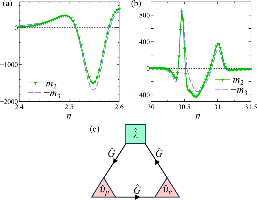
To understand the approximate relation , we consider the expansion of with respect to and ; . In this notation, and . To discuss the nature of the coefficient , we analyze the expression of based on the thermal Green function method derived in Ref. KotliarS :
| (S1) | |||||
where is the tight-binding Hamiltonian with finite , , is the velocity, and is the Green function. is the antisymmetric tensor, and with . The diagrammatic expression of Eq. [S1] is shown in Fig. S2 (c). The Hamiltonian of the site model,
| (S2) |
where is the Hamiltonian for and , where [] is the form factor of the current order [BO], which is given by the Fourier transform of [] introduced in the main text. [] () is the current order [BO] parameter. Then, the Green function is expanded as
| (S3) | |||||
where . Thus, the coefficient () can be derived from Eq. [S1], by expanding it with respect to () by using Eqs. [S2]-[S3].
Because of the relations
| (S4) | |||
| (S5) |
given by Eq. [S1] is zero for . Equations [S4] and [S5] are violated for because the current order form factor is odd-parity: . (Note that for the BO. Any Hermitian orders with the wavevector satisfy .) Thus, only odd-order terms with respect to can give nonzero .
Here, we consider in Eq. [S1] in the original 3-site unit cell picture. Then, the Green function in Eq. [S1] is expressed as , where and are matrices. The momentum is introduced by . To obtain finite , the total momenta introduced by , , should be (modulo original reciprocal vectors).
Hereafter, we discuss the reason for the relation . In this study, the nearest-neighbor order parameters are given in Fig. 1 (c) for the current order and Fig. 1 (a) for the BO. In the original 3-site unit cell picture, the relation () holds, where . For instance, we consider a term given by replacing , and with , and , respectively. The corresponding term is given by replacing with in . Due to the absence of sublattice hybridization around the vHS points Thomale2021S , is sublattice diagonal around the vHS points, that is, for . Then, the relation is satisfied approximately due to the relation with .
We have just started the analysis based on the Green function method. This is our important future issue.
C: Analysis of GL free energy with non-analytic -linear term
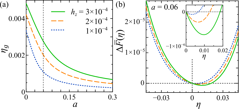
In the main text, we studied the strong interplay between the bond and current orders under the magnetic field in kagome metals. In Fig. 4, we studied the situation where bond order transition temperature is higher than the chiral current order one at . We revealed that chiral current order emerges at under . That is, the current-order transition temperature is enlarged to under small , as shown in Fig. 3 (b). The drastic field-induced current order originates from the non-analytic -linear terms in , that is, .
To understand the effect of the field-induced non-analytic free energy qualitatively, we analyze the following simple GL free energy with a -linear term:
| (S6) |
Here, we assume and are positive. When , is minimized at finite even if . The solution is given as
| (S7) | |||||
| (S8) |
Note that
| (S9) |
for small . Therefore, is finite even when due to the -linear term.
Here, we derive and from the GL free energy of kagome metal, Eqs. [11] and [10] in the main text. By setting and in Eqs. [11] and [10], we obtain and . When , , and , we get and . in Eq. [S6] corresponds to in the main text. In Fig. 3 (b) in the main text, we set with and , so in Fig. 4 (b) corresponds to in Eq. [S6].
Figure S3 (a) shows given in Eq. [S8] as a function of , in the case of and . We see that , which corresponds to T, induces sizable current order even above if . The obtained value of in Fig S3 (a) at is comparable to the field-induced order in Fig. 4 (b). The field-induced is prominent only when the system at is close to the current order state (i.e., ). Asymmetric as a function of is shown in Fig S3 (b).
D: Comparison between and
In the main text, we calculated the orbital magnetization in kagome metal with current order and bond-order using Eq. [3]. Next, we derived its expression up to the third-order of and : . To obtained the coefficients and , we calculate very accurately and expand it around numerically. For instance, we derive as with . (Note that if one of is zero.)
The expression is very useful to understand the strong interplay between current and bond orders in kagome metal. By considering the field-induced free energy , we understand the characteristic phase diagram of kagome metals under the magnetic field.
Here, we verify that in Eq. [8] well reproduces in Eq. [3]. Figures S4 (a)-(c) show the obtained results at under and as functions of , in the case of (a) , (b) and (b) . It is found that well reproduce the original when , unless the shape of the Fermi surface is drastically changed by order parameters.
Next, we examine the validity of the expansion expression in the realistic 30-orbital model for kagome metal. Figure S5 shows the coefficients and given by in Eq. [3] in the main text, derived from the region . The convergence of the obtained results for both and is good for for wide range of , except at the close vicinity of the vHS filling. Therefore, the GL free energy expression [9] in the main text is valid for real kagome metals.
E: in kagome lattice model with
In the main text, we studied in kagome lattice model with the bare hopping integrals and . The obtained coefficients and in take large values for , where is the van-Hove filling. Using the obtained coefficients and , we discovered the mechanism of the field-induced chiral current order in kagome metals.
To verify the robustness of the obtained results, here we analyze in kagome lattice model with large ; . The obtained FS shown in Fig. S6 (a) has large curvature due to large . Here, we have introduce the BO and the current order . Figure S6 (b) shows the obtained [] per atom due to the current order with . The relation is satisfied, and its magnitude is enlarged when . Figure S6 (c) shows [] due to the coexistence of current order and BO. The relation is satisfied when . Figures S6 (d) and (e) represent the obtained coefficients and in . The magnitudes of and for are comparable to those for given in the main text.
F: Calculation of GL parameters, Renormalization of
To verify that the GL free energy coefficients assumed in the main text are qualitatively reasonable, we calculate GL coefficients based on the diagrammatic method. The 4rh order GL parameters per unit cell are given as
| (S10) | |||||
| (S11) | |||||
| (S12) | |||||
| (S13) |
where
| (S14) | |||||
where is Green function for the original 3-site kagome lattice model and . The diagrammatic expression is depicted in Fig. S7 (a). is the form factor in the momentum space in the original BZ, or , and is 1, 2, or 3. Note that [] (=1-3) is given by the Fourier transform of [] introduced in the main text. The relation should be satisfied. Hereafter, we use derived from the density-wave equation in Ref. Tazai-kagome2S , in which distant-atom components are included. On the other and, is derived from the nearest-neighbor BO in Fig. 1 (a). In the same way, the analytic expressions of and are obtained in Ref. Tazai-kagome2S .
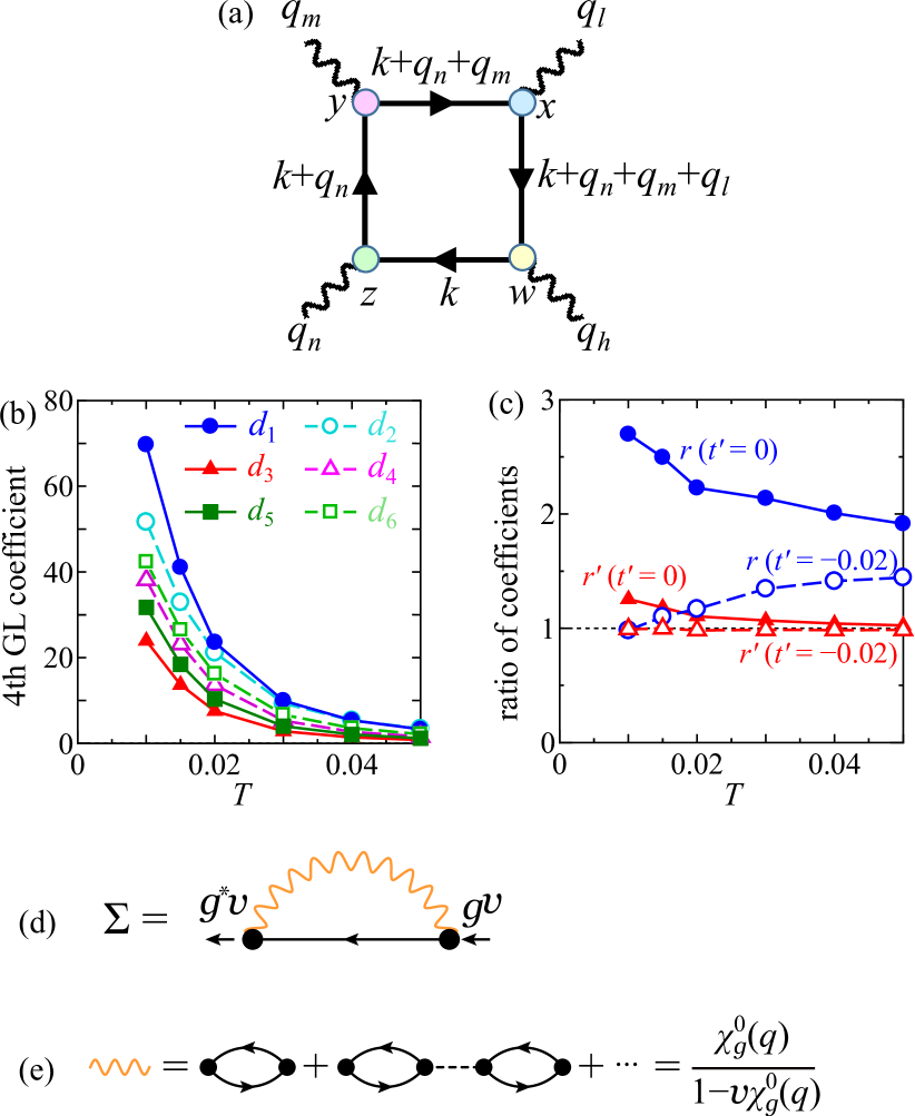
The obtained numerical results are given in Fig. S7 (b) for and . Here, the dimensionless form factors are normalized as . (This normalization corresponds to .) In the same way, we set . Thus, the parameter is consistent with Fig. S7 (b) for . For with , the 4th order term for the BO is [eV] for . The obtained ratios and are shown in Fig. S7 (c): For , we obtain and . For , and . Both ratios tend to become smaller than unity for larger . (Note that and when the form factors satisfy .)
In deriving in Fig. S7 (b), we included the self-energy due to the BO fluctuations Tazai-kagome2S , because the self-energy reduces unrealistic behaviors of at low temperatures when the inter-sublattice nesting vector is not exactly commensurate Balents2021S . (Note that the present method works well only for .) To calculate the self-energy, we introduce the following effective BO interaction Tazai-kagome2S :
| (S15) |
where is the BO operator Tazai-rev2021S ; Kontani-AdvPhysS ; Kontani-RPAS . and is the effective interaction. Here, the BO form factor is normalized as at each , ı.e., for the nearest sites. We next calculate the on-site self-energy due to BO fluctuations as Tazai-kagome2S
| (S16) | |||||
| (S17) |
which is shown in Fig. S7 (d). Here, the BO susceptibility is Tazai-kagome2S
| (S18) | |||||
| (S19) | |||||
| (S20) | |||||
which is shown in Fig. S7 (e). Then, the Green function is given as . The effect of thermal fluctuations described by the self-energy is essential to reproduce the -dependence of various physical quantities. In the present numerical study, we calculate Eqs. [S16]-[S20] self-consistently.
We also study the 2nd order GL term, which is derived as according to Ref. Tazai-LWS . Here, is the irreducible BO susceptibility, and , where is the eigenvalue of the density-wave equation, which is similar to the eigenvalue of the BCS gap equation. in usual BO phase transitions Tazai-LWS , while in BCS superconductivity because of large singularity of the p-p channel. As a result, for and . Note that corresponds to in the main text.
Therefore, the BO total free energy is for and . The current-order total free energy will be comparable to . Thus, the GL parameters assumed in the main text are qualitatively reasonable. (In BCS superconductors, when and .) As discussed in Ref. Tazai-LWS , the specific heat jump at the BO or current-order phase transition is much smaller than the BCS value .
Finally, we discuss the renormalization of the 2nd order GL coefficient for , , in the BO phase. Under the BO phase , in Eq. [11] is renormalized as due to the , terms. When , we obtain by neglecting term, which is allowed except for . Therefore, we obtain , where , , and . Here, we assume by referring to the relation in Fig. S7, owing to the difference between the BO and current order form factors. For detail, see Ref. Tazai-kagome2 .
G: by intra-original-unit-cell current order in kagome lattice
Here, we calculate in the case of the intra-original-unit-cell () current order in Fig. S8 (a). In this case, the translational symmetry is preserved. The obtained is shown in Fig. S8 (b). We find that is -linear even in the absence of the BO, while its coefficient is small for that is realized in kagome metals. Regardless of the presence of the -linear term in , field-induced intra-original-unit-cell order will be quite small in kagome metals. In fact, the field-induced cLC order at becomes sizable only when its second-order GL coefficient, , is very small. Here, is the eigenvalue of the current order solution at . However, the relation is obtained in the DW equation analysis in Ref. Tazai-kagome2S .
H: First principles -orbital model for kagome metal
In the main text, we analyzed the GL coefficients based on the first-principles 30-orbital model for kagome metals. Figure S9 (a) shows the obtained bandstructure in the plane. Its FS is shown in Fig. 5 (a). The -orbital “pure-type” band corresponds to the present three-orbital model. Its vHS energy is located at . Also, the -orbital forms the “mix-type” band, whose vHS energy is . In addition, the +-orbital forms a pure-type band with the vHS energy . Around M point, the -orbital band near M point is almost -independent, while other orbital bands exhibits small -independences (about ) in the band calculation.
Figure S9 (b) shows the bandstructure with introducing the -orbital shift eV. Its FS is shown in Fig. 5 (b). Here, the -orbital (mix-type) band approaches along the M-M’ line, consistently with the APRES measurement in Ref. ARPES-VHSS .
Here, we derive the coefficients and defined as , where and are the order parameter of a specific -orbital projected on the conduction band. The results for -orbital are shown in Figs. 5 (e)-(h) in the main text. (The weight of -orbital (, etc) on the conduction band is , , .) We also calculate and when the order parameters emerge on the , , and orbitals. The obtained results are shown in Figs. S9 (a) () and (b) (), as function of the electron filling . ( corresponds to undoped CsV3Sb5.) It is found that large and are obtained when the current and bond orders emerge on various -orbitals. Thus, the present study is valid for various types of current order mechanisms, not restricted to Ref. Tazai-kagome2S .
I: Increment of under uniaxial strain in BO phase
In Ref. Moll-hzS , it was proposed that CsV3Sb5 is located at the quantum critical point of the current order ( in the absence of the uniaxial strain. The field-induced (T) current order at K would be explained by the present theory. In addition, Ref. Moll-hzS reports the strain induced increment of in the absence of the magnetic field. It was explained in Ref. Moll-hzS based on the GL free energy analysis. Under the uniaxial strain, the degeneracy of the current order transition temperature at (), , is lifted. Then, will be larger than the original .
Here, we present that the strain induced change in the 4th order GL terms causes additional significant contribution to the increment of . That is, the BO-induced suppression of the current order is drastically reduced by the strain. Considering the symmetry, we assume that the symmetry strain induces the shift of the vHS energy levels as and . Then, the 4th order GL terms are given as
where and mod 3. When , for any and . Below, we show that each has large - and -linear terms when .
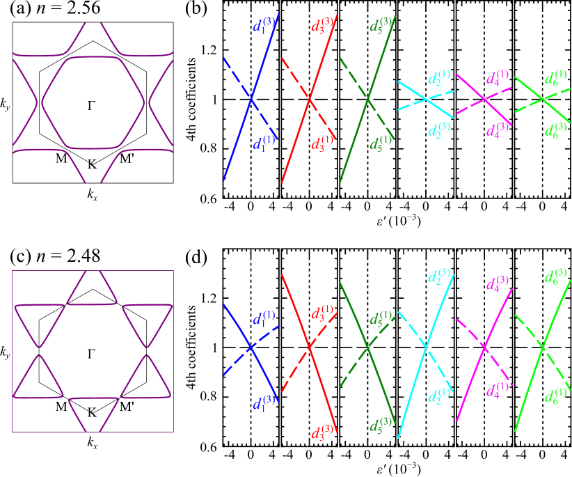
Here, we calculate the coefficients in the three-orbital model based on the Green function methods explained in the SI F. The used model parameters are , , , and . We first study the case of , whose FS at is shown in Fig. S10 (a). Figure S10 (b) shows the obtained normalized by its value, as functions of for . We also study the case of , whose FS at is shown in Fig. S10 (c). Figure S10 (d) shows the normalized as functions of . In both cases, the coefficients exhibits sizable -linear terms, by reflecting the large p-h asymmetry of the kagome lattice model.
In contrast, the irreducible susceptibility with the current form factor exhibit much smaller relative change in the same range of ; % for and % for . The form factor is introduced in the SI F. (The change in modifies the second order coefficient .) The change in the 3rd order term is very small, which is when .
Now, we consider the strain-induced change in the 4th order free energy term. By considering the symmetry property of the Feynman diagrams, due to is given as
| (S22) |
where are -linear. and are related as for =odd, and for =even. Also, due to is given as
| (S23) |
where are -linear. and are related as for =odd, and for =even.
Here, we consider the possible BO-current coexisting state motivated by the experiment in Ref. Moll-hzS . As explained in Ref. Tazai-kagome2S , in the case of at , the 3Q BO coexists with the current order due to the energy gain by the 3rd GL terms with . (The relation is general Tazai-kagome2S .) Then, the BO-current coexisting state is nematic. Here, we set (or ) without loss of generality.
Hereafter, we calculate the change in the current order transition temperature under the BO phase. (Below, we set for simplicity to obtain the analytic expression.) When , we obtain the square of the -th component of as ( and ), where . We consider by assuming . Then, the change in the free energy by of order is obtained as , where . In the present numerical study, and . (Exactly speaking, (0.29) for (2.48).)
In the BO phase at , the original 2nd order GL coefficient is changed by as
| (S24) | |||||
where when . For finite , it is changed by as
| (S25) | |||||
The current order appears in the BO phase when Eq. [S26] becomes negative. Therefore, will increase in proportion to if . (If , increases when .)
In the same way, is modified by as
| (S26) |
Note that and has the same sign according to Fig. S10, which is naturally expected analytically.
Considering the drastic -dependence of obtained in Fig. S10 (a), in collaboration with the change in already discussed in Ref. Moll-hzS , sizable strain-induced increment of the current order transition temperature reported in Ref. Moll-hzS will be realized in the present mechanism.
In the case of , and coincide with =even and =odd, respectively. Then, and . The main results are valid even in this case.
References
- (1) D. Ceresoli, T. Thonhauser, D. Vanderbilt, and R. Resta, Orbital magnetization in crystalline solids: Multi-band insulators, Chern insulators, and metals, Phys. Rev. B 74, 024408 (2006).
- (2) J. Shi, G. Vignale, D. Xiao, and Q. Niu, Quantum Theory of Orbital Magnetization and Its Generalization to Interacting Systems, Phys. Rev. Lett. 99, 197202 (2007).
- (3) R. Nourafkan, G. Kotliar, and A.-M. S. Tremblay, Orbital magnetization of correlated electrons with arbitrary band topology, Phys. Rev. B 90, 125132 (2014).
- (4) X. Wu, T. Schwemmer, T. Müller, A. Consiglio, G. Sangiovanni, D. Di Sante, Y. Iqbal, W. Hanke, A. P. Schnyder, M. M. Denner, M. H. Fischer, T. Neupert, and R. Thomale, Nature of Unconventional Pairing in the Kagome Superconductors (), Phys. Rev. Lett. 127, 177001 (2021).
- (5) R. Tazai, Y. Yamakawa,and H. Kontani, Charge-loop current order and nematicity mediated by bond-order Fluctuations in kagome metal AV3Sb5 (A= Cs,Rb,K), arXiv:2207.08068 (2022).
- (6) R. Tazai, Y. Yamakawa, M. Tsuchiizu, and H. Kontani, - and -wave quantum liquid crystal orders in cuprate superconductors, -(BEDT-TTF)2X, and coupled chain Hubbard models: functional-renormalization-group analysis, J. Phys. Soc. Jpn. 90, 111012 (2021).
- (7) T. Park, M. Ye, and L. Balents, Electronic instabilities of kagome metals: Saddle points and Landau theory, Phys. Rev. B 104, 035142 (2021).
- (8) H. Kontani, R. Tazai, Y. Yamakawa, and S. Onari, Unconventional density waves and superconductivities in Fe-based superconductors and other strongly correlated electron systems, Adv. Phys. 70, 355 (2021).
- (9) H. Kontani and S. Onari, Orbital-Fluctuation-Mediated Superconductivity in Iron Pnictides: Analysis of the Five-Orbital Hubbard-Holstein Model,P hys. Rev. Lett. 104, 157001 (2010).
- (10) R. Tazai, S. Matsubara, Y. Yamakawa, S. Onari, and H. Kontani, Rigorous formalism for unconventional symmetry breaking in Fermi liquid theory and its application to nematicity in FeSe, Phys. Rev. B 107, 035137 (2023).
- (11) Y. Hu, X. Wu, B. R. Ortiz, S. Ju, X. Han, J. Ma, N. C. Plumb, M. Radovic, R. Thomale, S. D. Wilson, A. P. Schnyder, and M. Shi, Rich nature of Van Hove singularities in Kagome superconductor CsV3Sb5, Nat. Commun. 13, 2220 (2022).
- (12) C. Guo, G. Wagner, C. Putzke, D. Chen, K. Wang, L. Zhang, M. G. Amigo, I. Errea, M. G. Vergniory, C. Felser, M. H. Fischer, T. Neupert, and P. J. W. Moll, Correlated order at the tipping point in the kagome metal CsV3Sb5, arXiv:2304.00972.