Multi-Armed Bandits with Generalized Temporally-Partitioned Rewards

Abstract

Decision-making problems of sequential nature, where decisions made in the past may have an impact on the future, are used to model many practically important applications. In some real-world applications, feedback about a decision is delayed and may arrive via partial rewards that are observed with different delays. Motivated by such scenarios, we propose a novel problem formulation called multi-armed bandits with generalized temporally-partitioned rewards. To formalize how feedback about a decision is partitioned across several time steps, we introduce $\beta$-spread property. We derive a lower bound on the performance of any uniformly efficient algorithm for the considered problem. Moreover, we provide an algorithm called TP-UCB-FR-G and prove an upper bound on its performance measure. In some scenarios, our upper bound improves upon the state of the art. We provide experimental results validating the proposed algorithm and our theoretical results.

1 Introduction

The classical multi-armed bandit (MAB, or simply bandit) problem is a framework to model sequential decision-making Bubeck and Cesa-Bianchi (2012a). In a MAB problem, the learning agent is faced with a finite set of $K$ arms, and a decision taken by the agent is symbolized by pulling an arm. Feedback about the decisions taken is available to the agent via numerical rewards. Multi-arm bandit literature typically focuses on scenarios where rewards are assumed to arrive immediately after pulling an arm. In contrast, the works on delayed-feedback bandits (e.g., Joulani et al. (2013); Mandel et al. (2015)) assume a delay between pulling an arm and the observation of its corresponding reward. In those studies, the reward is assumed to be concentrated in a single round that is delayed. This setting can be extended by allowing the reward to be partitioned into partial rewards that are observed with different delays. This type of bandit problem, known as MAB with Temporally-Partitioned Rewards (TP-MAB), was introduced by Romano et al. (2022).

In the TP-MAB setting, an agent will receive subsets of the reward over multiple rounds. The cumulative reward of an arm is the sum of the partial rewards obtained by pulling an arm. Romano et al. (2022) present $\alpha$-smoothness to characterize the reward structure. The $\alpha$-smoothness property states that the maximum reward in a group of consecutive partial rewards cannot exceed a fraction of the maximum reward (precise definition given in Definition 2). However, the assumption of $\alpha$-smoothness does not fit well if the cumulative reward is not uniformly spread. In this article, we introduce a more generalized way of formulating how an arm’s delayed cumulative reward is spread across several rounds.

As a motivating application, consider websites (e.g., Coursera, Khan Academy, edX) that provide Massive Open Online Courses (MOOCs). Such websites aim to provide users with useful recommendations for courses. This problem can be modeled as a TP-MAP problem. A course, which consists of a series of video lectures, might be thought of as an arm. A course can be recommended to a user by an agent, which corresponds to pulling an arm. When the student follows a course, the agent can observe partial rewards (e.g., by checking the watch time retention). In this setting, $\alpha$-smoothness rarely captures the actual cumulative reward distribution. Many students watch the video lectures at the beginning of a course but never finish the last few lectures, making the spread of partial rewards non-uniform. As a result, the existing work on delayed-feedback bandits and the algorithms proposed by Romano et al. (2022) may fail to recommend courses that are relevant for the user. Motivated by such scenarios, we investigate a more generalized way of formulating the reward structure.

Our Contributions

1. We introduce a novel MAB formulation with a generalized way of describing how an arm’s delayed cumulative reward is distributed across rounds.

2. We prove a lower bound on the performance measure of any uniformly efficient algorithm for the considered problem.

3. We devise an algorithm TP-UCB-FR-G and prove an upper bound on its performance measure. The proven upper bounds are tighter than the state of the art in some scenarios.

4. We provide experimental results that validate the correctness of our theoretical results and the effectiveness of our proposed algorithm.

2 Background and Related Work

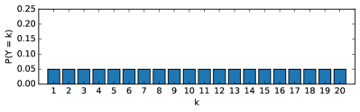
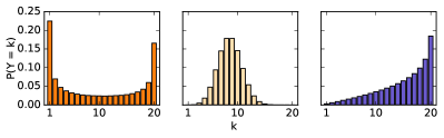
Figure 1: Probability distribution $\alpha$-smoothness (left) and possible probability distributions using our approach $\beta$-spread (right)

Online learning with delayed feedback is a well-studied problem in the literature. Owing to the space restrictions, a necessarily incomplete list of the works on this topic includes Weinberger and Ordentlich (2002); Agarwal and Duchi (2011); Mesterharm (2005, 2007); Desautels et al. (2014); Zinkevich et al. (2009). In the rest of this section, we focus on MAB with delayed feedback.

Joulani et al. (2013) studied the non-anonymous delayed feedback bandit problem and proposed a variant of the UCB algorithm Auer et al. (2002) as a solution. In Joulani et al. (2013), it is assumed that knowledge of which action resulted in a specific delayed reward is available. Wang et al. (2021) extend this problem to contain anonymous feedback and, in addition, eliminate the need for accurate prior knowledge of the reward interval. Recently, a variety of delayed-feedback scenarios were studied in MAB settings different from ours, such as linear and contextual bandits Arya and Yang (2020); Zhou et al. (2019); Vernade et al. (2020a), non-stationary bandits Vernade et al. (2020b). Furthermore, Pike-Burke et al. (2018) and Cesa-Bianchi et al. (2022) consider the case of delayed, aggregated, and anonymous feedback.

The majority of past research on the delayed MAB setting assumes that the entire reward of an arm is observed at once, either after some bounded delay Joulani et al. (2013); Mandel et al. (2015) or after random delays from an unbounded distribution with finite expectation Gael et al. (2020); Vernade et al. (2017). Our article studies the setting in which the reward for an arm is spread over an interval with a finite maximum delay value. This is consistent with the applications that we aim to model, such as MOOC providers mentioned in Section 1. To the best of our knowledge, Romano et al. (2022), were the first to analyze this setting. They introduced the Multi-Armed Bandit with Temporally-Partitioned Rewards (TP-MAB) setting. In the TP-MAB setting, a stochastic reward that is received by pulling an arm is partitioned over partial rewards observed during a finite number of rounds followed by the pull. Romano et al. (2022) assume that the arm rewards follow $\alpha$-smoothness property (precise definition given in Definition 2). As illustrated by the leftmost histogram in Figure 1, if an arm’s reward is $\alpha$-smooth, the probability of observing a partial reward in a group of consecutive rounds is uniformly partitioned.

While the study by Romano et al. (2022) provides promising results in the TP-MAB setting, it is based on the strong assumption that the $\alpha$-smoothness property holds. As a result, their proposed solutions are not suitable for a broader variety of scenarios where rewards are partitioned non-uniformly. As a remedy, we propose to use general distributions that can more accurately characterize how the received reward is partitioned. Consider a scenario in which additional information is available about how the cumulative reward is spread over the rounds. An example of such a scenario is a MOOC provider recommending courses to users, as described in Section 1. By generalizing the reward structure, our approach will be able to handle partitioned rewards in which the maximum reward per round is not partitioned uniformly across rounds, such as those shown on the right side of Figure 1.

Romano et al. (2022) introduce two novel algorithms based on the UCB algorithm that leverage $\alpha$-smoothness property: TP-UCB-EW and TP-UCB-FR. Both algorithms take an assumed $\alpha$ value as input and use it to calculate confidence terms similar to UCB Auer et al. (2002). Romano et al. (2022) showed that the TP-UCB-EW algorithm performs better with short time horizons $T$, whereas the TP-UCB-FR outperforms in the long run. Furthermore, they show that the cumulative regret of the TP-UCB-FR algorithm is greatly impacted by the assumed $\alpha$, whereas TP-UCB-EW only shows relatively minor changes in cumulative regret for different $\alpha$ values as input. Therefore, we believe that the setup of TP-UCB-FR is most suitable for leveraging assumed distribution in a generalized setting too. Subsequently, we use TP-UCB-FR as a baseline for our proposed algorithm.

3 Problem Formulation

Consider a MAB problem with $K$ arms over a time horizon of $T$ rounds, where $K,T\in\mathbb{N}$. At every round $t\in\{1,2,...,T\}$ an arm from the set of arms $\{1,2,...,K\}$ is pulled.

The performance of an algorithm $\mathfrak{A}$ after $T$ time steps for the considered problem can be measured using expected regret (or simply, regret) denoted as $\mathcal{R}_{T}(\mathfrak{A})$.

Definition 1.

(Regret) The regret of an algorithm $\mathfrak{A}$ after $T$ time steps is $\mathcal{R}_{T}(\mathfrak{A})\operatorname*{\coloneqq}\mu^{*}T-\sum_{i=1}^{K}\mu_{i}\cdot\mathbb{E}\left[N_{i}(T)\right]$, where $\mu^{*}\operatorname*{\coloneqq}\max_{1\leq i\leq K}\mu_{i}$ and $N_{i}(T)=$ number of times an arm $i$ is selected till time $t$.

The total reward is temporally partitioned over a set of rounds $T^{\prime}=\{t,t+1,...,t+\tau_{\max}-1\}$. Let $x^{i}_{t,m}(m\in T^{\prime})$ denote the partitioned reward that the learner receives at round $m$, after pulling the arm $i$ at round $t$. It is known to the agent which arm pull produced this reward. The cumulative reward is completely collected by the learner after a delay of at most $\tau_{\max}$. Each per-round reward $x^{i}_{t,m}$ is the realization of a random variable $X^{i}_{t,m}$ with support in $[0,\overline{X}^{i}_{m}]$. The cumulative reward collected by the learner from pulling arm $i$ at round $t$ is denoted by $r^{i}_{t}$ and it is the realization of a random variable $R^{i}_{t}$ such that $R^{i}_{t}:=\sum_{n=t}^{t+\tau_{\max}-1}X^{i}_{t,n}$ with support $[0,\overline{R}^{i}]$. Straightforwardly, we observe that $\overline{R}^{i}:=\sum_{n=t}^{\tau_{\max}}\overline{X}^{i}_{n}$.

Romano et al. (2022) have shown that, in practice, per-round rewards for an arm provide information on the cumulative reward of the arm. Romano et al. (2022) introduce an $\alpha$-smoothness property (defined in Definition 2) that partitions the temporally-spaced rewards such that each partition corresponds to the sum of a set of consecutive per-round rewards. Formally, let $\alpha\in T^{\prime}$ be such that $\alpha$ is a factor of $\tau_{\max}$. The cardinality of each partition, which we shall name ‘$z$-group’ from now on, is denoted by $\phi:=\frac{\tau_{\max}}{\alpha}$ with $\phi\in\mathbf{N}$. Similar to above, we can now define each $z$-group $z^{i}_{t,k},k\in\{1,2,...,\alpha\}$ as the realization of a random variable $Z^{i}_{t,k}$ such that for every $k$:

$$Z^{i}_{t,k}:=\sum_{n=t+(k-1)\phi}^{t+k\phi-1}X^{i}_{t,n}$$ (1)

such that $Z^{i}_{t,k}$ has support $[0,\overline{Z}^{i}_{\alpha,k}]$.

Definition 2 ($\alpha$-smoothness).

For $\alpha\in\{1,...,\tau_{max}\}$, the reward is $\alpha$-smooth iff $\frac{\tau_{max}}{\alpha}$ $\in\mathbb{N}$ and for each $i\in\{1,...,K\}$ and $k\in\{1,2,...,\alpha\}$ the random variables $Z_{t,k}^{i}$ are independent and s.t. $\overline{Z}_{\alpha,k}^{i}=\overline{Z}_{\alpha}^{i}=\frac{\overline{R}^{i}}{\alpha}$.

The $\alpha$-smoothness property ensures that all temporally-partitioned rewards contribute towards bounding the values of future rewards within the same window. If the $\alpha$-smoothness holds, then the maximum cumulative reward in a $z$-group $\overline{Z}_{\alpha,k}^{i}$ is equal for all $z$-groups $k\in\{1,2,...,\alpha\}$. Therefore, we can say that $\forall_{k}\in\{1,2,...,\alpha\}$, $\overline{Z}_{\alpha,k}^{i}=\overline{Z}_{\alpha}^{i}$.

However, the assumption of $\alpha$-smoothness is unsuitable for scenarios in which the cumulative reward is not evenly partitioned across rounds. To fit such scenarios, the goal of this article is to generalize the spread of the rewards across $z$-groups. To that end, one has to eliminate the assumption that every $z$-group has an equal probability of attaining a partial reward. To accomplish this, we replace $\alpha$-smoothness with $\beta$-spread property that allows for modeling scenarios in which the cumulative reward is not distributed uniformly across rounds i.e, a property that allows $\overline{Z}_{\alpha,k}^{i}$ to differ across $z$-groups.

3.1 Our Solution approach: $\beta$-spread property

Let us consider that for each partial reward, we have a discrete random variable $Y$ that represents the index of the $z$-group in which the partial reward will be observed. The set of all possible values that $Y$ can take is therefore $\{1,2,...\alpha\}$. Each possible value of $Y$ is associated with a certain probability that signifies the probability that the partial reward will be observed in $z$-group $k$. This means a non-uniform spread of rewards over the $z$-groups is possible. Formally, we define this concept of $\beta$-spread as follows:

Definition 3 ($\beta$-spread).

Let $Y$ be a discrete random variable representing the index of the $z$-group in which a partial reward will be observed. $Y$ has a discrete probability distribution $\mathbb{F}$ with a finite domain of size $\alpha$ that is defined by a probability mass function denoted by $P_{\mathbb{F}}(k)$ for $k\in\{1,,\dots,\alpha\}$. We say that a reward of arm $i$ is $\beta$-spread if the partial rewards of arm $i$ are distributed according to an arbitrary discrete distribution $\mathbb{F}$. The upper bounds for the $z$-groups for every $k,i$ are defined as:

$$\overline{Z}_{\alpha,k}^{i}=P_{\mathbb{F}}(k)\cdot\overline{R}^{i}$$ (2)

Based on prior information about how the cumulative reward is distributed over the rounds, the reward spread can be defined by any fitting probability distribution $\mathbb{F}$ as long as it adheres to the definition of $\beta$-spread. For example, beta-binomial distributions with a range starting from 1 and ending at $\alpha$ could be used to describe reward spread. The histograms on the right side of Figure 1 depict a few of these Beta-Binomial distributions with varying shape parameters, but the possibilities for choosing other parameters or distributions matching scenarios we aim to model are nearly inexhaustible.

4 Lower Bound on Regret

Using the $\beta$-spread property, we can derive the following lower bound for a uniformly efficient policy i.e., any policy with regret in $o(T^{x})$ with $x<1$.

Theorem 1.

The regret of any uniformly efficient policy $\mathfrak{U}$ applied to the TP-MAB problem with the $\beta$-spread property after $T$ time steps is lower bounded as

$$\lim\inf_{T\rightarrow+\infty}\frac{\mathcal{R}_{T}(\mathfrak{U})}{\ln T} \geq\sum_{i:\mu_{i}<\mu^{*}}\frac{2}{(\alpha+1)}\operatorname{\sum_{k=1}^{\alpha}kB(k)}$$

$$\qquad\cdot\alpha\operatorname{\sum_{k=1}^{\alpha}\left(B(k)\right)^{2}}\frac{\Delta_{i}}{\alpha\mathcal{KL}\left(\frac{\mu_{i}}{\bar{R}_{\max}},\frac{\mu^{*}}{R_{\max}}\right)}$$

where $\Delta_{i}\operatorname*{\coloneqq}\mu^{*}-\mu_{i}$ and $\mathcal{KL}(p,q)\operatorname*{\coloneqq}$ Kullback-Leibler divergence between Bernoulli random variables with means p and q.

Comparison with the Lower Bound given by Romano et al. (2022)

By assuming $\alpha$-smoothness, Romano et al. (2022) proved the following lower bound for TP-MAB:

$$\lim\inf_{T\rightarrow+\infty}\frac{\mathcal{R}_{T}(\mathfrak{U})}{\ln T}\geq\sum_{i:\mu_{i}<\mu^{*}}\frac{\Delta_{i}}{\alpha\mathcal{KL}\left(\frac{\mu_{i}}{\bar{R}_{\max}},\frac{\mu^{*}}{R_{\max}}\right)}.$$ (3)

Note that our lower bound given in Theorem 1 resolves to the lower bound given by Romano et al. (2022) in Eq.(3) in case of $\alpha$-smoothness. However, our lower bound for the considered problem setting is tighter when

$$\frac{2}{(\alpha+1)}\operatorname{\sum_{k=1}^{\alpha}kB(k)}\cdot\alpha\operatorname{\sum_{k=1}^{\alpha}\left(B(k)\right)^{2}}>1.$$

Proof Sketch for Theorem 1

We start by constructing two MAB problem instances that call for different behaviors from the algorithm attempting to solve them. Then, we use the change-of-distribution argument to show that any uniformly efficient algorithm cannot efficiently distinguish between these instances.

The complete proof for Theorem 1 is given in Appendix A.

5 Proposed Algorithm and Regret Upper Bound

In this section, we propose an algorithm that makes use of the $\beta$-spread property in the TP-MAB setting and prove an upper bound on its regret.

5.1 Proposed Algorithm: TP-UCB-FR-G

Our proposed algorithm, called TP-UCB-FR-G, is an extension of the algorithm TP-UCB-FR given by Romano et al. (2022). In TP-UCB-FR-G, the most significant modification is the confidence interval $c^{i}_{t-1}$ which is rigorously built to suit the $\beta$-spread property.

Algorithm 1 TP-UCB-FR-G

1:  $\textbf{Input: }\alpha\in[\tau_{max}],\tau_{max}\in\mathbb{N}^{*},B\sim Y$

2:  for $t\in\{1,...,K\}$ do

3:     Pull an arm $i_{t}=t$

4:  end for

5:  for $t\in\{K+1,...,T\}$ do

6:     for $t\in\{1,...,K\}$ do

7:        Compute $\hat{R}_{t-1}^{i}$ and $c_{t-1}^{i}$ as in (4) and (5)

8:        $u_{t-1}^{i}\leftarrow\hat{R}_{t-1}^{i}+c_{t-1}^{i}$

9:     end for

10:     Pull arm $i_{t}=z=\operatorname*{argmax}_{i\in[K]}u_{t-1}^{i}$

11:     Observe $x_{h,t-h+1}^{i_{h}}$ for $h\in\{t-\tau_{max}+1,...,t\}$

12:  end for

As input, the algorithm takes a smoothness constant $\alpha\in[\tau_{max}]$, a maximum delay $\tau_{max}$ and a probability mass function $B$. The algorithm uses $B$ to be able to give a proper judgment of an arm before all the delayed partial rewards are observed. This is realized by replacing the not yet received partial rewards with fictitious realizations, or in other words, the expected estimated rewards.

At round $t$, the fictitious reward vectors are associated with each arm pulled in the span $H:=\{t-\tau_{max}+1,...,t-1\}$. These fictitious rewards are denoted by $\tilde{\boldsymbol{x}}_{h}^{i}=\left[\tilde{x}_{h,1}^{i},\ldots,\tilde{x}_{h,\tau_{\max}}^{i}\right]$ with $h\in H$, where $\tilde{x}_{h,j}^{i}:=x_{h,j}^{i}$, if $h+j\leq t$ (the reward has already been seen), and $\tilde{x}_{h,j}^{i}=0$, if $h+j>t$ (the reward will be seen in the future). The corresponding fictitious cumulative reward is $\tilde{r}_{h}^{i}:=\sum_{j=1}^{\tau_{\max}}\tilde{x}_{h,j}^{i}$.

In the initialization phase of the algorithm (lines 2-4), each arm is pulled once. Later, at each time step $t$, the upper confidence bounds $u_{t-1}^{i}$ are determined for each arm $i$ by computing the estimated expected reward $\hat{R}_{t-1}^{i}$ and confidence interval $c_{t-1}^{i}$ using Eq. (4) and (5) respectively.

$$\hat{R}_{t-1}^{i}:=\frac{1}{N_{i}(t-1)}\left(\sum_{h=1}^{t-\tau_{\max}}r_{h}^{i}\mathbb{I}_{\left\{i_{h}=i\right\}}+\sum_{h\in H}\tilde{r}_{h}^{i}\mathbb{I}_{\left\{i_{h}=i\right\}}\right).$$ (4)

where $N_{i}(t-1):=\sum_{h=1}^{t-1}\mathbb{I}_{\left\{i_{h}=i\right\}}$ is the number of times arm $i$ has been pulled up to round $t-1$.

$$c_{t-1}^{i} =\frac{\phi\bar{R}^{i}}{N_{i}(t-1)}\sum_{k=1}^{\alpha}kB(k)$$

$$\qquad+\bar{R}^{i}\sqrt{\frac{2\ln(t-1)\sum_{k=1}^{\alpha}\left(B(k)\right)^{2}}{N_{i}(t-1)}}.$$ (5)

The algorithm then pulls the arm $i$ with the highest upper confidence bound $u_{t-1}^{i}$ and observes its rewards.

5.2 Regret Upper Bound of TP-UCB-FR-G

Theorem 2.

In the TP-MAB setting with $\beta$-spread reward, the regret of TP-UCB-FR-G after $T$ time steps with B(k) matching the PMF $P_{\mathbb{F}}(k)$ of random variable $Y$ is upper bounded as

$$\mathcal{R}_{T}(\texttt{TP-UCB-FR-G})\leq\sum_{i:\mu_{i}<\mu^{*}}\frac{4\ln T\operatorname{(\bar{R}^{i})^{2}\sum_{k=1}^{\alpha}\left(B(k)\right)^{2}}}{\Delta_{i}}$$

$$\quad\qquad\cdot\left(1+\sqrt{1+\frac{\Delta_{i}\phi\operatorname{\sum_{k=1}^{\alpha}kB(k)}}{\bar{R}^{i}\ln T\sum_{k=1}^{\alpha}\left(B(k)\right)^{2}}}\right)$$

$$\quad\qquad+2\phi\operatorname{\sum_{k=1}^{\alpha}kB(k)}\sum_{i:\mu_{i}<\mu^{*}}\bar{R}^{i}+\left(1+\frac{\pi^{2}}{3}\right)\sum_{i:\mu_{i}<\mu^{*}}\Delta_{i}$$

Observe that $\operatorname{\sum_{k=1}^{\alpha}kB(k)}=\operatorname{\mathbb{E}}[Y]$, meaning the expected value of our random spread variable $Y$ influences the upper bound of the algorithm. Another interesting factor is $\sum_{k=1}^{\alpha}\left(B(k)\right)^{2}$. This factor can be seen as an approximation of the index of coincidence Friedman (1987) between rewards. The index of coincidence determines the probability of two reward points being observed in the same $z$-group. Its minimal value equals $\frac{1}{\alpha}$ and occurs when the $\alpha$-smoothness property holds (uniform distribution). The value is maximal and equal to 1 if all rewards fall into one $z$-group.

5.2.1 Comparison with the Upper Bound of TP-UCB-FR given in Romano et al. (2022)

Let us compare our upper bound given in Theorem 2 with the upper bound given in Romano et al. (2022). For the latter bound to hold, the $\alpha$ estimate given as input to their algorithm has to match the $\alpha$ of the real reward distribution as well. Note that $\operatorname{\mathbb{E}}[Y]=\frac{\alpha+1}{2}$ in case of $\alpha$-smoothness. For $Y\sim\mathbb{F}$ with $\operatorname{\mathbb{E}}[Y]<\frac{\alpha+1}{2}$ our upper bound on the regret is lower. Furthermore, choosing a $\beta$-spread distribution $\mathbb{F}$ with a low mean and a low index of coincidence will result in a better upper bound using Theorem 2 compared to choosing $\mathbb{F}$ with rewards centered towards the end (high mean) and not spread out (high index of coincidence).

5.2.2 Proof Sketch of Theorem 2

Here we provide a proof sketch for Theorem 2. The complete proof can be in Appendix B.

The approach can be divided into three steps. Firstly, we show that the probability that an optimal arm is estimated significantly lower than its mean is bounded by $t^{-4}$. Secondly, we show the probability of a suboptimal arm being estimated significantly higher than its mean is bounded by $t^{-4}$. Finally, we evaluate how the algorithm performs in distinguishing the difference between the optimal and suboptimal arms.

6 Experimental Results

In this section, we compare our proposed algorithm TP-UCB-FR-G with TP-UCB-FR Romano et al. (2022), UCB1 Auer et al. (2002), and Delayed-UCB1 Joulani et al. (2013). We observe how well TP-UCB-FR-G performs in settings with different reward distributions. We use the experimental settings proposed by Romano et al. (2022). That is, two synthetically generated environments and a real-world playlist recommendation scenario. In these settings, we inherit learners used in the provided experiments in Romano et al. (2022), and create new learner configurations using TP-UCB-FR-G. As input distributions for the new learners, we use Beta-Binomial distributions with unique parameter values for each learner. The Beta-Binomial distribution gives us the opportunity to model extreme scenarios, which should result in more insightful experimental results. We observe that other distributions do not grant the flexibility of a Beta-Binomial distribution, as demonstrated in experiments deferred to Appendix C.4. In the plots under this section, we use the notation TP-UCB-FR-G$(\alpha,\texttt{dist\_name})$ to denote a learner for our algorithm, where dist_name is the name of the Beta-Binomial distribution for which the exact parameters are shown in Table 1. Additional details about the used Beta-Binomial distributions and experimental settings are given in Appendix C.4.

Distribution name	$\alpha$	$\beta$
extreme_begin	1	100
very_begin	1	16
begin	2	8
begin_middle	2	4
middle	5	5
middle_end	4	2
end	8	2
very_end	16	1

Table 1: Parameter values for Beta-Binomial distributions

Setting 1: Uniform Reward Distribution

In this setting, we evaluate the influence of $\alpha$ on TP-UCB-FR-G. We set $K=10$, $\tau_{\max}=100$ rounds, and the maximum reward such that it is more difficult for a learner to converge to the optimal arm, by letting $\overline{R}^{i}=100\zeta^{i}$ where $\zeta\in\{1,3,6,9,12,15,18,21,22,23\}$. The aggregate rewards are s.t. $Z^{i}_{t,k}\sim\frac{\overline{R}^{i}}{\alpha}U[0,1]$, and we use a setting $\alpha$-smoothness constant of $\alpha=20$. We run the algorithm over a time horizon $T=10^{5}$, and average the results over $100$ independent runs. We run the setting for $\alpha_{est}\in\{5,10,20,25,50\}$, where $\alpha_{est}$ is the estimation of the $\alpha$-smoothness constant. To mimic real-world applications where the underlying data generating distribution and $\alpha$ values are possibly unknown, we use $\alpha_{est}$ to estimate this constant.

Results

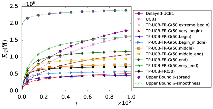
Figure 2: Regret against time for Setting 1 with $\alpha_{est}=50$

Let us focus on the results for $\alpha_{est}=50$. Its performance is plotted against time in Figure 2, along with the theoretical upper-bounds for the corresponding setting. Note that the upper-bounds for $\beta$-spread and $\alpha$-smoothness are equal, which is expected in this setting with uniform spread. The high upper bound at low values for $t$ is caused by constants in the upper-bound equation, which are dependent on the experimental set-up. The maximum cumulative reward of the arms is the most dominant factor. First, note that it has been shown by Romano et al. (2022) that optimistic (large) values for $\alpha_{est}$ lead to better performance in practice. However, overly optimistic values for $\alpha_{est}$ do not necessarily lead to better performance. Thus, TP-UCB-FR is largely influenced by the mis-specification of $\alpha_{est}$. Note that the learners TP-UCB-FR-G$(50,\texttt{begin})$ and TP-UCB-FR-G$(50,\texttt{begin\_middle})$ perform significantly better than the TP-UCB-FR learner proposed by Romano et al. (2022). In fact, TP-UCB-FR-G$(50,\texttt{begin})$ and TP-UCB-FR-G$(50,\texttt{begin\_middle})$ are approximately asymptotically parallel to TP-UCB-FR, granting significant performance gains for higher time horizons $T$ as well. This implies that our contribution improves the performance bound in the setting by Romano et al. (2022).

Further results show that, for lower $\alpha_{est}$ values, TP-UCB-FR-G learners with begin-oriented distributions perform slightly better. In the specific case of $\alpha_{est}=5$, numerical analysis of the exact regret results deferred to Appendix C, shows that our proposed learner TP-UCB-FR-G$(5,\texttt{begin\_middle})$ performs $\approx 4.5\%$ better than the TP-UCB-FR learner by Romano et al. (2022). Furthermore, as $\alpha_{est}$ starts to increase, the performance of begin-oriented TP-UCB-FR-G learners increases faster than that of TP-UCB-FR, resulting in an improvement of $\approx 22.1\%$ for $\alpha_{est}=20$, and to $\approx 36.1\%$ for $\alpha_{est}=50$. We observe that TP-UCB-FR-G$(\alpha_{est},\texttt{begin})$ is essentially the ’ideal’ learner, since it always delivers better performance than the learner by Romano et al. (2022) in the tested settings. These results suggest that the issue of being overly/underly optimistic is essentially inherited from the setting by Romano et al. (2022) in a different shape. Overly-optimistic TP-UCB-FR-G learners perform worse in general. This can be attributed to the fact that overly-optimistic learners generally have an assumed distribution with a high index of coincidence, because the rewards are assumed to be more concentrated at the beginning or at the end. The indices of coincidence for the ’extreme begin’ and ’very end’ learners in Setting 1 with $\alpha_{est}=50$ are $\approx 0.51$ and $0.14$, respectively. These are significantly higher than $\approx 0.05$, for both the ’begin’ and the ’end’ learner in the same setting. Similarly, underly-optimistic learners with a middle-oriented distribution also perform poorly. This can be explained by the expected value of their assumed distributions, which is higher than the begin-oriented distributions as indicated by their name.

Setting 2: Non-Uniform Reward Distributions

The second setting aims to test the performance of the TP-UCB-FR-G algorithm in scenarios where the distribution of the aggregate reward over the time steps after an arm pull is non-uniform. The distribution of rewards in this setting are s.t. $Z^{i}_{t,k}\sim\frac{\overline{R}^{i}}{\alpha}Beta[a^{i}_{k},b^{i}_{k}]$ where $Beta$ is a Beta distribution with $a,b$ s.t. rewards are distributed according to the spread of the corresponding setting. Again, we model $K=10$ arms, an $\alpha$-smoothness constant of $\alpha=20$ and a maximum reward s.t. convergence to an optimal arm takes longer. That is, $\overline{R}^{i}=100\zeta^{i}$ with $\zeta\in\{1,3,6,9,12,15,18,21,22,23\}$. However, there is a difference in the $\tau_{\max}$, $\alpha_{est}$ and the parameters used for the assumed Beta distribution by the learners. The exact configurations can be found in Appendix C. In general, there are 12 combinations consisting of 4 configurations with 3 scenarios each. The configurations differ in $\tau_{\max}$ and $\alpha_{est}$, whereas the scenarios differ in distribution parameters. Generally, there is one uniform scenario (equal to Setting 1), one where the rewards are observed late after the pull (Setting 2.1), and one where the results are observed just after the pull (Setting 2.2). We use learners with the same estimated distributions as in Setting 1 (see Table 1).

Results

Running the proposed Setting 2.1 and 2.2 for $\tau_{\max}=100$ and $\alpha_{est}=50$ produces results that are visually identical to the results from Setting 1 given in Figure 2. However, analysis of the numerical results reveals that differences exist. The cumulative regret generally increases slightly from Setting 2.2 to Setting uniform and then to Setting 2.1.

Figure 3: Differences in cumulative regret between scenarios for learners in Setting 2 with $\tau_{\max}=100,\alpha_{est}=50$

In Figure 3, we illustrate the differences in cumulative regret between settings where aggregate rewards are distributed non-uniformly. Let us denote $\Delta(s_{1},s_{2})$ for $s_{1},s_{2}\in\{\texttt{Setting 2.1},\texttt{Setting 2.2},\texttt{Uniform}\}$ as the absolute difference in cumulative regret between Settings $s_{1}$ and $s_{2}$. Note that the differences presented in Figure 3 are only marginal. For example, $\Delta(\texttt{Setting 2.1},\texttt{Setting 2.2})\approx 4.8\times 10^{3}$ for learner TP-UCB-FR-G$(50,\texttt{very\_end})$ which is the highest difference in average regret observed across all compared settings. Since the regret of TP-UCB-FR-G$(50,\texttt{very\_end})$ averaged over $T$ is $\approx 1.61\times 10^{6}$, the observed change of $\approx 0.3\%$ is neglectable. Furthermore, the same experiment performed with different values for both $\tau_{\max}$ and $\alpha_{est}$ seems to confirm the same marginal change. As an example, Setting 2 for $\tau_{\max}=200$ and $\alpha_{est}=20$ results in a maximum change in average regret of only $\approx 0.5\%$.
These results suggest that the performance of TP-UCB-FR-G learners in a setting where aggregate rewards are distributed uniformly is indistinguishable from a setting where aggregate rewards are distributed non-uniformly. Therefore, we can align with the conclusion of Setting 1; TP-UCB-FR-G$(\alpha,\texttt{begin})$ delivers a significant performance increase compared to the learner proposed by Romano et al. (2022). The gain that we observe for the mentioned settings is as high as $\approx 48.2\%$. An extensive performance summary is deferred to Appendix C. Again, due to the flexibility of choice for a distribution, there is potential for even higher performance gains.

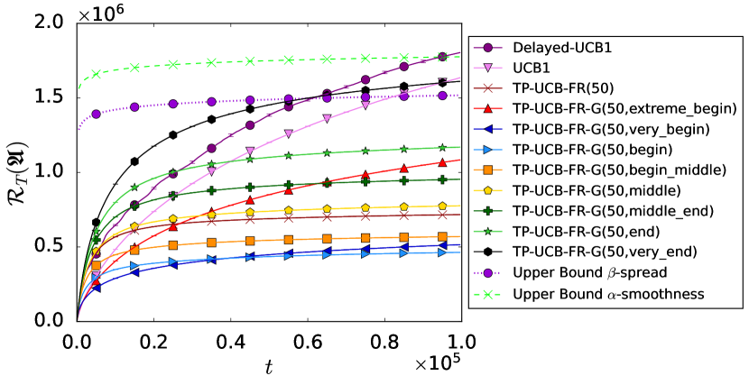
Figure 4: Regret against time for Setting 2.2 with $\tau_{\max}=100$ and $\alpha_{est}=50$

In Figure 4, the theoretical upper bound of TP-UCB-FR-G as well as the the upper bound of the TP-UCB-FR algorithm is plotted on top of the results for the Setting 2.2. The figure shows that the upper bound proposed in this article is tighter in this setting. Note that the theoretical upper bounds for TP-UCB-FR-G and TP-UCB-FR only hold for specific learners that assume the data generating distribution precisely and that the ’very end’ learner exceeds the $\beta$-spread upper bound. This shows another reason to estimate the assumed distribution optimistically.

User recommendations: Spotify Playlists

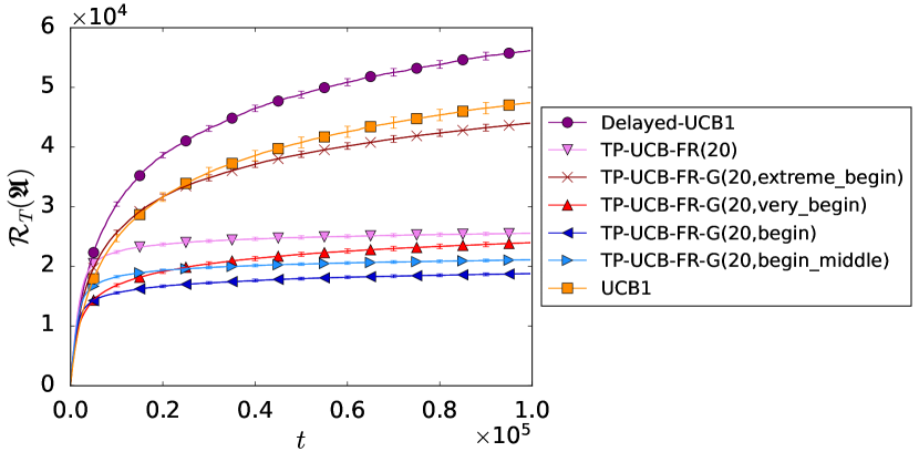
Figure 5: Regret against time for begin-oriented learners in the Spotify Setting

To verify our algorithm on a real-world dataset, we solve the user recommendation problem introduced by Romano et al. (2022), using the Spotify dataset introduced in Brost et al. (2019). We select the $K=6$ most played playlists as the arms to be recommended. Each time a playlist $i$ is selected, the corresponding reward realizations $x^{i}_{t}$ for the first $N=20$ songs are sampled from the dataset. In this setting, the $\alpha$-smoothness is $\alpha=20$, the maximum delay $\tau_{\max}=4N=80$ and the results are averaged over $100$ independent runs.

Results

In Figure 5, we observe that optimistic learners significantly outperform the learner TP-UCB-FR$(20)$ introduced by Romano et al. (2022). Let us focus on the learner TP-UCB-FR-G$(20,\texttt{begin})$, since it is by far the best performing learner. We observe that this learner has a decrease of $\approx 26.3\%$ in regret, averaged over the time horizon $T$, when compared to TP-UCB-FR$(20)$. Table 2 provides a complete summary of the performance gains of TP-UCB-FR-G learners in the Spotify setting.

Learner	Regret	Decrease
TP-UCB-FR-G$(\alpha_{est}=20)$	($\times 10^{4}$)	(%)
extreme_begin	4.40	$\approx-72.5$
very_begin	2.40	$\approx 5.9$
begin	$\boldsymbol{1.88}$	$\boldsymbol{\approx 26.3}$
begin_middle	2.11	$\approx 17.2$

Table 2: TP-UCB-FR-G Learners and their decrease in regret compared to the regret of TP-UCB-FR$(20)=2.55\times 10^{4}$

A second observation we make is that, aligning with the conclusion from Setting 1, overly-optimistic learners such as TP-UCB-FR-G(20,extreme_begin) perform significantly worse than TP-UCB-FR$(20)$. As shown in Table 2, the average regret increases by $\approx 72.5\%$. Nevertheless, since TP-UCB-FR-G$(20,\texttt{begin})$ performs significantly better than TP-UCB-FR$(20)$ for larger $t$, it is even better suited to provide playlist recommendations.

7 Concluding Remarks and Future Work

In this article, we model sequential decision-making problems with delayed feedback using a novel formulation called multi-armed bandits with generalized temporally-partitioned rewards. To generalize delayed reward distributions, we introduce the $\beta$-spread property. A lower bound for this TP-MAB setting with the $\beta$-spread property is provided that can be tighter than the lower bound for the TP-MAB setting with the $\alpha$-smoothness property. More specifically, we show that even when $\alpha$ is equal for both settings, a high mean or high index of coincidence for the assumed distribution leads to a tighter bound in the setting introduced in this article. We also introduce the TP-UCB-FR-G algorithm that exploits the $\beta$-spread property and show that in certain scenarios the upper bound of this algorithm can be lower than the upper bound of the TP-UCB-FR algorithm, and therefore also lower than the upper bounds of the classical UCB1 and Delayed-UCB1 algorithms. Finally, we empirically show that our algorithm outperforms TP-UCB-FR and other UCB algorithms over a wide range of experiments with synthetic and real-world data. The decrease in cumulative regret reaches 26.3% against the state of the art TP-UCB-FR algorithm in the experiment with real-world data.

Directions for future work include:

1. Currently, the $\beta$-spread property is restricted to discrete probability distributions bounded by a finite domain of size $\alpha$. An interesting future research topic could be to look into the removal of these restrictions, as this could lead to more flexibility in our algorithm, and broaden its practical applications.

2. Another possible extension could be to consider settings in which the arms are treated as subsets, such that each subset of arms is assigned different $\alpha$-values and distributions. This could be advantageous in settings where arms are treated as clusters e.g., the setting by Pandey et al. (2007)

3. Moreover, another interesting topic is to look at scenarios where the time span over which the reward is partitioned i.e., $\tau_{\max}$, is variable. In our current work, we assume it to be fixed and consistent across arms. Removing this assumption could be beneficial if we want to consider practical applications where $\tau_{\max}$ is not fixed, such as observing the reward of an online advertisement (clicks on the advertisement) over the lifetime ($\tau_{\max}$) of that advertisement, which is variable.

Appendix A Proof of Theorem 1

Proof.

The proof follows along the lines of the proof of Theorem 2.2 from Bubeck and Cesa-Bianchi [2012b], which is based on Lai and Robbins [1985]. Because the $\beta$-spread property has no effect on the cardinality $\phi$ of the $z$-groups, we can generalize to a setting where multiple rewards are earned by a single arm pull. Let us define an auxiliary TP-MAB setting in which:

• only two arms exist with expected values $\mu_{1}$ and $\mu_{2}$ s.t. $\mu_{2}<\mu_{1}<1$.

• upper bound on the reward for each arm is equal to the maximum upper bound, i.e., $\overline{R}^{i}_{t}=\overline{R}_{\max}$

• The total rewards in each $z$-group, $Z^{i}_{t,k}$, are independent, and the expected value of the rewards in each $z$-group is $\mathrm{B}(k)\cdot\mu_{i}$.

• The total reward in $z$-group, $Z^{i}_{t,k}$, is a scaled Bernoulli random variable s.t. $Z^{i}_{t,k}\in\{0,\mathrm{B}(k)\cdot\overline{R}_{\max}\}$

• Pulling an arm at time $t$ provides rewards $\{Z^{i}_{t,1},...,Z^{i}_{t,\alpha}\}$ that can all be observed immediately at the time of the pull.

In this proof of the lower bound, we trivially observe that finding the optimal arm in a setting in which all of the partial rewards are observed at once can never be more difficult than in a setting in which rewards are spread out over a set of rounds $\{t,t+1,...,\tau_{max}\}$. As a result, a lower bound in this defined setting corresponds to a lower bound in our $\beta$-spread setting.

To give an idea of how good an arm is compared to its maximum, we derive a new alternative mean for each arm as $\mu_{A_{i}}=\frac{\mu_{i}}{\overline{R}_{\max}}$. Note that $\mu_{A_{i}}<1$ as mentioned before.

Let $\mathbb{E}[\mathrm{N}_{i}(T)]$ denote the expected number of times an arm $i$ is pulled over a set of rounds $T$. To compute $\mathbb{E}[\mathrm{N}_{1}(\{t,t+1,...,\tau_{max}\})]$ and $\mathbb{E}[\mathrm{N}_{2}(\{t,t+1,...,\tau_{max}\})]$, we can use the scaled reward values without loss of validity. If we now consider a second, modified instance of the above TP-MAB setting, with the only difference being that arm 2 is now the optimal arm s.t. $\mu_{A_{1}}<\mu^{\prime}_{A_{2}}<1$, we can show that the learning agent choosing the arms cannot distinguish between the different instances. This reasoning implies a lower bound on the number of times a suboptimal arm is played. We know that $x\mapsto\mathcal{KL}(\mu_{A_{1}},x)$ is a continuous function, and we can find a $\mu^{\prime}_{A_{2}}$ for each $\epsilon>0$, such that:

$$\mathcal{KL}(\mu_{A_{2}},\mu^{\prime}_{A_{2}})\leq(1+\epsilon)\mathcal{KL}(\mu_{A_{2}},\mu_{A_{1}})$$ (6)

The proof follows the steps given in the work by Bubeck and Cesa-Bianchi [2012b] to derive a lower bound for any uniform policy $\mathfrak{U}$.

Step 1: $\mathbb{P}(C_{t})=o(1)$

For this proof, we change the notation of the rewards slightly such that each variable in the sequence $Z^{i}_{1,1},...,Z^{i}_{n,\alpha}$ represents the cumulative reward of an arm $i$ when pulled $n$ times, at timestep $k\in\{1,2,...,\alpha\}$. $Z^{i}_{s,k}$ for $s\in\{1,2,...,n\}$ represents the cumulative reward of an arm $i$ after the $s$’th pull at timestep $k$ after a pull. Using this notation, we can define the empirical estimate of $\mathcal{KL}(\mu_{Z_{2}},\mu^{\prime}_{Z_{2}})$ as:

$$\widehat{\mathcal{KL}}_{\alpha\beta}:=\sum_{n=1}^{s}\sum_{k=1}^{\alpha}\mathrm{ln}\frac{\mu_{A_{2}}Z^{2}_{n,k}+(1-\mu_{A_{2}})(1-Z^{2}_{n,k})}{\mu^{\prime}_{A_{2}}Z^{2}_{n,k}+(1-\mu^{\prime}_{A_{2}})(1-Z^{2}_{n,k})}$$

Using this, we define an event that links the behavior of the original agent to the modified version

$$C_{t}\operatorname*{\coloneqq}\left\{\alpha N_{2}(t)<f_{t}\quad\text{ and }\quad\widehat{\mathcal{KL}}_{\alpha N_{2}(t)}\leq(1-\varepsilon/2)\ln t\right\}$$ (7)

with

$$f_{t}=\left(\frac{2}{\alpha+1}\operatorname{\sum_{k=1}^{\alpha}kB(k)}\cdot\alpha\operatorname{\sum_{k=1}^{\alpha}\left(B(k)\right)^{2}}\right)\frac{1-\epsilon}{\mathcal{KL}(\mu_{A_{2}},\mu^{\prime}_{A_{2}})}\ln t$$

Using the change of measure identity defined in Bubeck and Cesa-Bianchi [2012b] and the second inequality in the definition of $C_{t}$ given in Eq. (7):

$$\mathbb{P}^{\prime}\left(C_{t}\right)=\mathbb{E}\left[1_{C_{t}}\exp\left(-\widehat{\mathcal{KL}}_{\alpha N_{2}(t)}\right)\right]\geq e^{-(1-\varepsilon/2)\ln t}\mathbb{P}\left(C_{t}\right)$$

Then, we first rearrange the terms of the above inequality to obtain

$$\mathbb{P}\left(C_{t}\right) \leq t^{(1-\varepsilon/2)}\mathbb{P}^{\prime}\left(C_{t}\right)$$

$$\leq t^{(1-\varepsilon/2)}\mathbb{P}^{\prime}\left(\alpha N_{2}(t)<f_{t}\right)$$

$$\leq t^{(1-\varepsilon/2)}\frac{\mathbb{E}^{\prime}\left[t-N_{2}(t)\right]}{t-f_{t}/\alpha}$$

$$=o(1)$$

In the equations above, we use $\mathbb{P}^{\prime}\left(C_{t}\right)\leq\mathbb{P}^{\prime}\left(\alpha N_{2}(t)<f_{t}\right)$, Markov’s inequality and the fact that the policy $\mathfrak{U}$ is uniformly efficient (i.e. $\operatorname{\mathbb{E}}[N_{2}(t)]=o(t^{\gamma})$ with $\gamma<1$).

Step 2: $\mathbb{P}\left(\alpha N_{2}(t)\leq f_{t}\right)=o(1)$

Using Theorem 2.2 from Bubeck and Cesa-Bianchi [2012b] and observing that we always have

1. $\operatorname{\sum_{k=1}^{\alpha}kB(k)}\geq 1\implies\frac{2}{\alpha+1}\operatorname{\sum_{k=1}^{\alpha}kB(k)}\geq\frac{2}{\alpha+1}$

2. $\operatorname{\sum_{k=1}^{\alpha}\left(B(k)\right)^{2}}\in[\frac{1}{\alpha},1]\implies\alpha\operatorname{\sum_{k=1}^{\alpha}\left(B(k)\right)^{2}}\in[1,\alpha]$

3. $\frac{2}{\alpha+1}\operatorname{\sum_{k=1}^{\alpha}kB(k)}\cdot\alpha\operatorname{\sum_{k=1}^{\alpha}\left(B(k)\right)^{2}}\geq\frac{2}{(\alpha+1)}>0$

Next, we define two events

$$E_{1}=\alpha N_{2}(t)<f_{t}$$

and

$$E_{2} =\biggl{(}\frac{\alpha+1}{2\alpha}\cdot\frac{1}{\operatorname{\sum_{k=1}^{\alpha}kB(k)}\cdot\operatorname{\sum_{k=1}^{\alpha}\left(B(k)\right)^{2}}}\cdot$$

$$\frac{\mathcal{KL}\left(\mu_{Z_{2}},\mu_{Z_{2}}^{\prime}\right)}{(1-\varepsilon)\ln t}\cdot\max_{\beta<f_{t}/\alpha}\widehat{\mathcal{KL}}_{\alpha\beta}$$

$$\leq\frac{1-\varepsilon/2}{1-\varepsilon}\cdot\frac{\alpha+1}{2\alpha}\cdot\frac{\mathcal{KL}(\mu_{Z_{2}},\mu_{Z_{2}}^{\prime})}{\operatorname{\sum_{k=1}^{\alpha}kB(k)}\cdot\operatorname{\sum_{k=1}^{\alpha}\left(B(k)\right)^{2}}}\biggr{)}$$

such that we obtain:

$$o(1) =\mathbb{P}\left(C_{t}\right)\leq\mathbb{P}(E_{1}\wedge E_{2})$$

Using the strong law of large numbers for the event $E_{2}$ s.t. $\lim_{t\rightarrow+\infty}\mathbb{P}\left(E_{2}\right)=1$, we can conclude that $\mathbb{P}\left(E_{1}\right)=\mathbb{P}\left(\alpha N_{2}(t)<f_{t}\right)=o(1)$, and that for $t\rightarrow+\infty$ we have $\mathbb{E}\left[N_{2}(t)\right]>f_{t}/\alpha$.

Final Step

Using Equation (6) we know that, for $t\rightarrow+\infty$ :

$$\mathbb{E}\left[N_{2}(t)\right] >f_{t}/\alpha$$

$$=\frac{2}{\alpha+1}\operatorname{\sum_{k=1}^{\alpha}kB(k)}\cdot\alpha\operatorname{\sum_{k=1}^{\alpha}\left(B(k)\right)^{2}}$$

$$\qquad\frac{1-\varepsilon}{\alpha\mathcal{KL}\left(\mu_{A_{2}},\mu_{A_{2}}^{\prime}\right)}\ln t$$

$$\geq\frac{2}{\alpha+1}\operatorname{\sum_{k=1}^{\alpha}kB(k)}\cdot\alpha\operatorname{\sum_{k=1}^{\alpha}\left(B(k)\right)^{2}}$$

$$\qquad\frac{1-\varepsilon}{\alpha(1+\varepsilon)\mathcal{KL}\left(\mu_{A_{2}},\mu_{A_{1}}\right)}\ln t$$

where the theorem statement is derived from the arbitrariness of the value of $\varepsilon$, substituting $\mu_{A_{1}}$ with $\frac{\mu^{*}}{\bar{R}_{\max}}$ and $\mu_{A_{2}}$ with $\frac{\mu_{2}}{\bar{R}_{\max}}$, and summing over all the sub-optimal arms. ∎

Appendix B Proof of Theorem 2

B.1 Preliminaries

The relation between the expected amount of sub-optimal arm pulls and the regret of the algorithm is given by

$$\mathcal{R}_{T}(\texttt{TP-UCB-FR-G})=\sum_{i:\mu_{i}<\mu^{*}}\Delta_{i}\mathbb{E}\left[N_{i}(T)\right]$$

Let us define the true empirical mean of the cumulative reward of arm $i$ computed over $N_{i}(t)$ arm pulls:

$$\hat{R}_{t}^{i,\text{ true }}:=\frac{1}{N_{i}(t)}\sum_{h=1}^{t}r_{h}^{i}\mathds{1}_{\left\{i_{h}=i\right\}}$$

The value above assumes that the cumulative reward of an arm pull is known, even if partial rewards are still to come in the future. We bound the difference between the true empirical mean and the observed empirical mean as follows:

$$\hat{R}_{t}^{i,\text{ true }}-\hat{R}_{t}^{i}$$

$$=\frac{1}{N_{i}(t)}\sum_{h=1}^{t}\sum_{j=1}^{\tau_{\max}}\left(x_{h,j}^{i}-\tilde{x}_{h,j}^{i}\right)\mathds{1}_{\left\{i_{h}=i\right\}}$$

$$\leq\frac{1}{N_{i}(t)}\sum_{h=1}^{t}\sum_{j=1}^{\tau_{\max}}(x_{h,j}^{i}-\tilde{x}_{h,j}^{i})$$

$$=\frac{1}{N_{i}(t)}\sum_{h=\max\left\{1,t-\tau_{\max}+2\right\}}^{t}\sum_{j=t-h+2}^{\tau_{\max}}x_{h,j}^{i}$$ (8)

$$\leq\frac{1}{N_{i}(t)}\sum_{k=1}^{\alpha}k\phi\bar{R}^{i}B(k)$$ (9)

$$=\frac{\phi\bar{R}^{i}}{N_{i}(t)}\sum_{k=1}^{\alpha}kB(k)$$ (10)

Eq. (8) states that the difference between the true and observed mean equals the sum of all future rewards that are yet to be observed for a maximum of $\tau_{\max}-1$ arms that have been pulled. The closer index $h$ gets to the current time $t$, the more pulled arms exist with unobserved rewards. Therefore, the amount of reward that is unobserved can be bounded by looping over all $z$-groups in Eq. (9) to calculate the maximum reward still to be observed and giving higher weight to late $z$-groups through index $k$. Furthermore, Eq. (9) holds because of the $\beta$-spread property.

Fact 1 (Hoeffding inequality Hoeffding [1963]).

Let $X_{1},\ldots,X_{n}$ be random variables in $[0,1]$ such that $\mathbb{E}\left[X_{t}\mid X_{1},\ldots,X_{t-1}\right]=\mu$. Let $S_{n}=X_{1}+\cdots+X_{n}$. Then, for all $a\geq 0$

$$\quad\mathbb{P}\left\{S_{n}\leq n\mu-a\right\}\leq e^{-2a^{2}/n}.$$

Deriving the upper bound

By construction of the algorithm TP-UCB-FR-G, the upper bound on the expected number of times a suboptimal arm $i$ is pulled can be expressed as follows:

$$\mathbb{E}\left[N_{i}(t)\right]\leq\ell+\sum_{t=1}^{\infty}\sum_{s=1}^{t-1}\sum_{s_{i}=\ell}^{t-1}\mathbb{P}\left\{\left(\hat{R}_{t,s}^{*}+c_{t,s}^{*}\right)\leq\left(\hat{R}_{t,s_{i}}^{i}+c_{t,s_{i}}^{i}\right)\right\}$$ (11)

where $\hat{R}_{t,s}^{*}$ and $c_{t,s}^{*}$ are the empirical mean and the confidence term of the optimal arm and $\hat{R}_{t,s_{i}}^{i}$ and $c_{t,s_{i}}^{i}$ denote the empirical mean and the confidence term for arm $i$.

For (11) to hold, one of the following three inequalities have to hold as well:

$$\hat{R}_{t,s}^{*}\leq\mu^{*}-c_{t,s}^{*}$$ (12)

$$\hat{R}_{t,s_{i}}^{i}\geq\mu_{i}+c_{t,s_{i}}^{i}$$ (13)

$$\mu^{*}<\mu_{i}+2c_{t,s_{i}}^{i}$$ (14)

Let us pay attention to (12) first and find the following:

$$\mathbb{P}\left(\hat{R}_{t,s}^{*}-\mu^{*}\leq-c_{t,s}^{*}\right)$$

$$=\mathbb{P}\left(\hat{R}_{t,s}^{*\text{ true }}-\mu^{*}\leq-c_{t,s}^{*}+\hat{R}_{t,s}^{*\text{ true }}-\hat{R}_{t,s}^{*}\right)$$

$$\leq\mathbb{P}\left(\hat{R}_{t,s}^{*\text{ true }}-\mu^{*}\leq-c_{t,s}^{*}+\frac{\phi\bar{R}^{i}}{s}\sum_{k=1}^{\alpha}kB(k)\right)$$

$$=\mathbb{P}\left(s\hat{R}_{t,s}^{*\text{ true }}\leq s\mu^{*}-s\sqrt{\frac{2\ln t\sum_{k=1}^{\alpha}\left(\bar{R}^{*}B(k)\right)^{2}}{s}}\right)$$

$$\leq\exp\left\{-\frac{\left(2\sqrt{\frac{2\ln t\sum_{k=1}^{\alpha}\left(\bar{R}^{*}B(k)\right)^{2}}{s}}\right)^{2}s^{2}}{\sum_{l=1}^{s}\sum_{k=1}^{\alpha}\left(\bar{R}^{*}B(k)\right)^{2}}\right\}$$

$$\leq e^{-4\ln t}$$

$$=t^{-4}$$

where we use Hoeffding’s inequality (defined in Fact 1), the penultimate step and $c_{t,s_{i}}^{i}\operatorname*{\coloneqq}\frac{\phi\bar{R}^{i}}{s}\sum_{k=1}^{\alpha}kB(k)+\bar{R}^{i}\sqrt{\frac{2\ln t\sum_{k=1}^{\alpha}\left(B(k)\right)^{2}}{s}}$

Similarly, the bound from (13) can be derived:

$$\mathbb{P}\left(\hat{R}_{t,s_{i}}^{i}-\mu_{i}\geq c_{t,s_{i}}^{i}\right) \leq\mathbb{P}\left(\hat{R}_{t,s}^{i,\text{ true }}-\mu_{i}\geq\bar{R}^{i}\sqrt{\frac{2\ln t}{\alpha s_{i}}}\right)$$

$$\leq e^{-4\ln t}$$

$$=t^{-4}$$

where we use Hoeffding’s inequality (defined in Fact 1) and the fact that by definition $\hat{R}_{t,s_{i}}^{i}\leq\hat{R}_{t,s_{i}}^{i,true}$. All that is left to do is to consider Eq. (14). Let us assume that Eq. (14) does not hold i.e., $\mu^{*}\geq\mu^{i}+2c^{i}_{t,s}$. This is equivalent to

$$\Delta_{i}\geq 2\left(\frac{\phi\bar{R}^{i}}{s_{i}}\sum_{k=1}^{\alpha}kB(k)+\sqrt{\frac{2\ln t\sum_{k=1}^{\alpha}\left(\bar{R}^{*}B(k)\right)^{2}}{s_{i}}}\right)$$

Rearranging the terms.

$$\frac{\Delta_{i}^{2}}{4}+\frac{\phi^{2}(\bar{R}^{i})^{2}}{s_{i}^{2}}\left(\sum_{k=1}^{\alpha}kB(k)\right)^{2}-2\left(\frac{\Delta_{i}\phi(\bar{R}^{i})}{2s_{i}}\left(\sum_{k=1}^{\alpha}kB(k)\right)\right)$$

$$\geq\frac{2\ln t\sum_{k=1}^{\alpha}\left(\bar{R}^{*}B(k)\right)^{2}}{s_{i}}$$

$$s_{i}^{2}\frac{\Delta_{i}^{2}}{4}+\phi^{2}(\bar{R}^{i})^{2}\left(\sum_{k=1}^{\alpha}kB(k)\right)^{2}-2s_{i}\bigg{(}\frac{\Delta_{i}\phi(\bar{R}^{i})}{2}\left(\sum_{k=1}^{\alpha}kB(k)\right)$$

$$\qquad+\ln t\sum_{k=1}^{\alpha}\left(\bar{R}^{*}B(k)\right)^{2}\bigg{)}$$

$$\geq 0$$

By solving for $s_{i}$, the following can be established:

$$s_{i} \geq\frac{2\phi\bar{R}^{i}\operatorname{\sum_{k=1}^{\alpha}kB(k)}}{\Delta_{i}}+\frac{4\ln t\operatorname{(\bar{R}^{i})^{2}\sum_{k=1}^{\alpha}\left(B(k)\right)^{2}}}{\Delta_{i}^{2}}$$

$$\qquad+4\frac{\sqrt{\left(\ln t\operatorname{(\bar{R}^{i})^{2}\sum_{k=1}^{\alpha}\left(B(k)\right)^{2}}\right)\left(1+\frac{\operatorname{\sum_{k=1}^{\alpha}kB(k)}\Delta\phi\bar{R}^{i}}{\ln t\operatorname{(\bar{R}^{i})^{2}\sum_{k=1}^{\alpha}\left(B(k)\right)^{2}}}\right)}}{\Delta_{i}^{2}}$$

$$s_{i} \geq\frac{2\phi\bar{R}^{i}\operatorname{\sum_{k=1}^{\alpha}kB(k)}}{\Delta_{i}}+\left(\frac{4\ln t\operatorname{(\bar{R}^{i})^{2}\sum_{k=1}^{\alpha}\left(B(k)\right)^{2}}}{\Delta^{2}_{i}}\right)$$

$$\quad\cdot\left(1+\sqrt{1+\frac{\Delta_{i}\phi\bar{R}^{i}\operatorname{\sum_{k=1}^{\alpha}kB(k)}}{\ln t\operatorname{(\bar{R}^{i})^{2}\sum_{k=1}^{\alpha}\left(B(k)\right)^{2}}}}\right)$$

As a result, we pick

$$l =\Biggl{\lceil}\frac{2\phi\bar{R}^{i}\operatorname{\sum_{k=1}^{\alpha}kB(k)}}{\Delta_{i}}+\left(\frac{4\ln t\operatorname{(\bar{R}^{i})^{2}\sum_{k=1}^{\alpha}\left(B(k)\right)^{2}}}{\Delta^{2}_{i}}\right)$$

$$\qquad\cdot\left(1+\sqrt{1+\frac{\Delta_{i}\phi\bar{R}^{i}\operatorname{\sum_{k=1}^{\alpha}kB(k)}}{\ln t\operatorname{(\bar{R}^{i})^{2}\sum_{k=1}^{\alpha}\left(B(k)\right)^{2}}}}\right)\Biggr{\rceil}$$

to ensure that the inequality in Eq. (14) is always false for $s_{i}\geq l$.

$$\mathbb{E}\left[N_{i}(t)\right]$$

$$\leq\Biggl{\lceil}\frac{2\phi\bar{R}^{i}\operatorname{\sum_{k=1}^{\alpha}kB(k)}}{\Delta_{i}}+\left(\frac{4\ln t\operatorname{(\bar{R}^{i})^{2}\sum_{k=1}^{\alpha}\left(B(k)\right)^{2}}}{\Delta^{2}_{i}}\right)$$

$$\qquad\cdot\left(1+\sqrt{1+\frac{\Delta_{i}\phi\bar{R}^{i}\operatorname{\sum_{k=1}^{\alpha}kB(k)}}{\ln t\operatorname{(\bar{R}^{i})^{2}\sum_{k=1}^{\alpha}\left(B(k)\right)^{2}}}}\right)\Biggr{\rceil}$$

$$\qquad+\sum_{t=1}^{\infty}\sum_{s=1}^{t-1}\sum_{s_{i}=\ell}^{t-1}\left[\mathbb{P}\left(\hat{R}_{t,s}^{*}-\mu^{*}\leq-c_{t,s}^{*}\right)\right]$$

$$\qquad+\sum_{t=1}^{\infty}\sum_{s=1}^{t-1}\sum_{s_{i}=\ell}^{t-1}\left[\mathbb{P}\left(\hat{R}_{t,s_{i}}^{i}-\mu_{i}\geq c_{t,s_{i}}^{i}\right)\right]$$

$$\leq\frac{2\phi\bar{R}^{i}\operatorname{\sum_{k=1}^{\alpha}kB(k)}}{\Delta_{i}}+\left(\frac{4\ln t\operatorname{(\bar{R}^{i})^{2}\sum_{k=1}^{\alpha}\left(B(k)\right)^{2}}}{\Delta^{2}_{i}}\right)$$

$$\qquad\cdot\left(1+\sqrt{1+\frac{\Delta_{i}\phi\bar{R}^{i}\operatorname{\sum_{k=1}^{\alpha}kB(k)}}{\ln t\operatorname{(\bar{R}^{i})^{2}\sum_{k=1}^{\alpha}\left(B(k)\right)^{2}}}}\right)$$

$$\qquad+1+\sum_{t=1}^{\infty}\sum_{s=1}^{t-1}\sum_{s_{i}=\ell}^{t-1}2t^{-4}$$

$$\leq\frac{2\phi\bar{R}^{i}\operatorname{\sum_{k=1}^{\alpha}kB(k)}}{\Delta_{i}}+\left(\frac{4\ln t\operatorname{(\bar{R}^{i})^{2}\sum_{k=1}^{\alpha}\left(B(k)\right)^{2}}}{\Delta^{2}_{i}}\right)$$

$$\qquad\cdot\left(1+\sqrt{1+\frac{\Delta_{i}\phi\bar{R}^{i}\operatorname{\sum_{k=1}^{\alpha}kB(k)}}{\ln t\operatorname{(\bar{R}^{i})^{2}\sum_{k=1}^{\alpha}\left(B(k)\right)^{2}}}}\right)$$

$$\qquad+1+\frac{\pi^{2}}{3}$$

The theorem statement follows by the fact that $\mathcal{R}_{T}\left(\mathfrak{U}_{\mathrm{FR}}\right)=\sum_{i:\mu_{i}<\mu^{*}}\Delta_{i}\mathbb{E}\left[N_{i}(T)\right]$.

Appendix C Experimental Environment Details

C.1 Technical Details

The code has been executed on a server configured with 2 Intel Xeon 4110 2.1Ghz (32 hyperthreads) CPU’s and 384GB RAM. We did not make use of GPU acceleration during the simulation process. The operating system used is Ubuntu 16.04.7 LTS. The code for the simulations is created in Python with version 3.9.12. Furthermore, we use Conda for library management, and for the experiments, the following libraries are used:

• numpy 1.23.4

• pandas 1.5.1

• tqdm 4.64.1

• scipy 1.9.3

• matplotlib 3.5.3

Because this research is partially based on the findings by Romano et al. [2022], we used their code as a base and made adaptations to run the experiments for our learners. Overall, running all settings takes approximately 96 hours on the hardware mentioned above.

C.2 TP-UCB-FR-G learner configurations

We introduce new learners to the experimental settings using a variant of the Beta-Binomial distribution. A brief introduction to the Beta-Binomial distribution itself will be provided first, followed by the introduction of our variation. For a more complete overview of Beta-Binomial distributions, we refer to Lee [2012].
Let $N\in\mathbb{N}$, $\alpha\in\mathbb{R}^{+}$ and $\beta\in\mathbb{R}^{+}$, and note that $\alpha$ in this setting is some arbitrary constant instead of a spread parameter as it is in the rest of this article. For $x\in\{0,..,N\}$, the probability mass function is then defined as

$$BetaBinom(N,\alpha,\beta)(x)=\binom{N}{x}\frac{B(x+\alpha,N-x+\beta)}{B(\alpha,\beta)}$$ (15)

where the $B(u,v)$ is the beta function for some $u,v\in\mathbb{R}^{+}$. As can be seen, the domain of the distribution is not equal to the $\alpha$-sized domain of $\{1,2,\dots,\alpha\}$ required for the $\beta$-spread property to hold. Therefore, we create a variant of the Beta-Binomial distribution that is in this domain in Equation 16.

$$BetaBinomVariant(x)=BetaBinom(\alpha-1,a,b)(x-1)$$ (16)

where $\alpha$ denotes the amount of $z$-groups and a and b are the distribution parameters. The domain of this function is the desired interval of all integers $\{1,2,\dots,\alpha\}$. Note that formulas for calculating the mean or variance do not hold anymore for this variant. For each experimental setting, we add 8 synthetic learners that are distributed according to this variant. Their exact parameters are given in Table 1, and the corresponding probability mass functions are also plotted in Figure 6. Note that the distribution names are chosen according to their ’center’ on the $x$–axis. That is, the location on the $x$-axis with the highest observed probability.

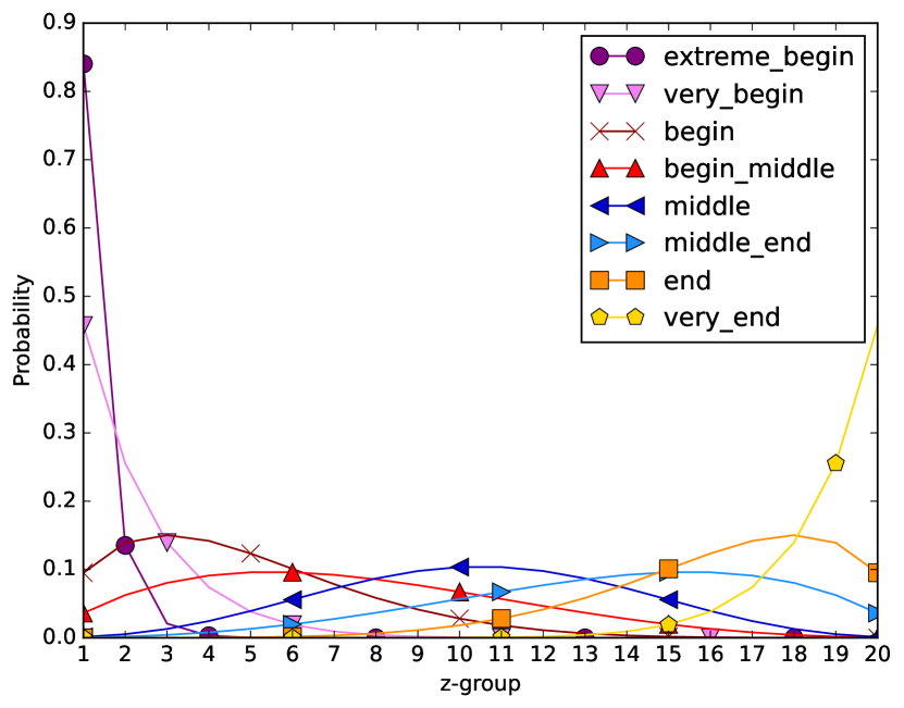
Figure 6: Probability mass functions for different Beta-Binomial configurations

C.3 Experimental Settings

In this section, we detail the experiment settings presented in Section 6 and some further experiments that have been run to confirm the results in the main article.

C.3.1 Setting 1

The primary goal of this setting is to discover the influence of adjusting $\alpha$ over TP-UCB-FR-G learners. We run this setting for different choices of $\alpha$, $\alpha_{est}\in[5,10,20,25,50]$. In this setting, we model $k=10$ arms, the reward is collected over $\tau_{\max}=100$ rounds, and the maximum reward is set to be $\overline{R}^{i}=100i$. The aggregate rewards for the learner proposed in Romano et al. [2022] are s.t. $Z^{i}_{t,k}\sim\frac{\overline{R}^{i}}{\alpha}U[0,1]$. TP-UCB-FR-G learners in this setting assume a different aggregate rewards structure such that $Z^{i}_{t,k}\sim\frac{\overline{R}^{i}}{\alpha}Beta(a^{i}_{k},b^{i}_{k})$. The experiment is run over a time horizon $T=10^{5}$, and the $\alpha$-smoothness constant is $\alpha=20$. The results are averaged over $100$ independent runs.
Section 6 provides the results for $\alpha_{est}=50$. In this section, let us focus on the results of TP-UCB-FR-G when $\alpha_{est}=[5,10,20,25]$. These results are plotted in Figures 7, 8, 9 and 10 respectively. These results align with the conclusions from Section 6. That is, as $\alpha_{est}$ increases, begin-centered learners perform increasingly better than other learners. For $\alpha_{est}=5$, we see that the begin_middle learner performs better for larger $t$. This indicates that, in case of lower $\alpha_{est}$ values, begin is too optimistic.

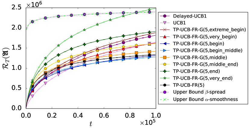
Figure 7: Regret against time for Setting 1 with $\alpha_{est}=5$

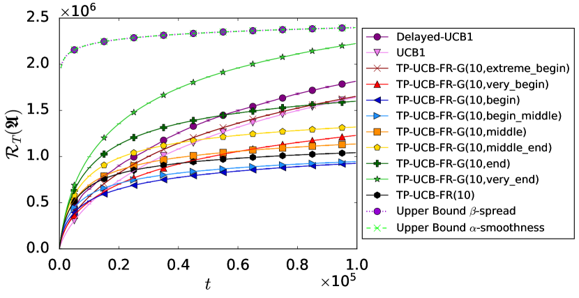
Figure 8: Regret against time for Setting 1 with $\alpha_{est}=10$

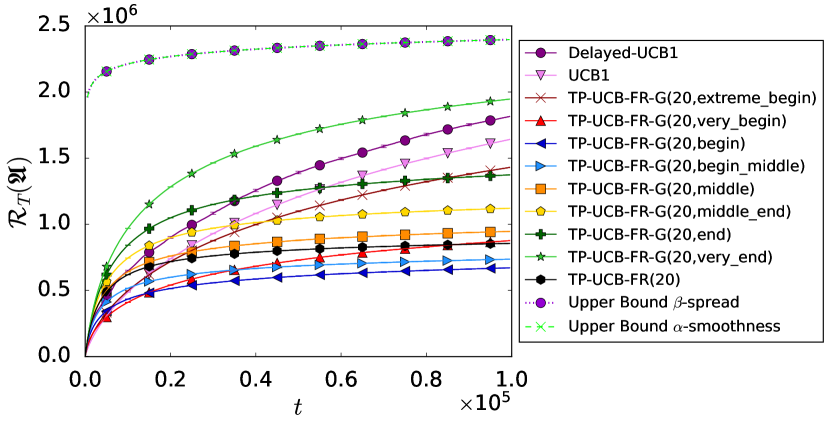
Figure 9: Regret against time for Setting 1 with $\alpha_{est}=20$

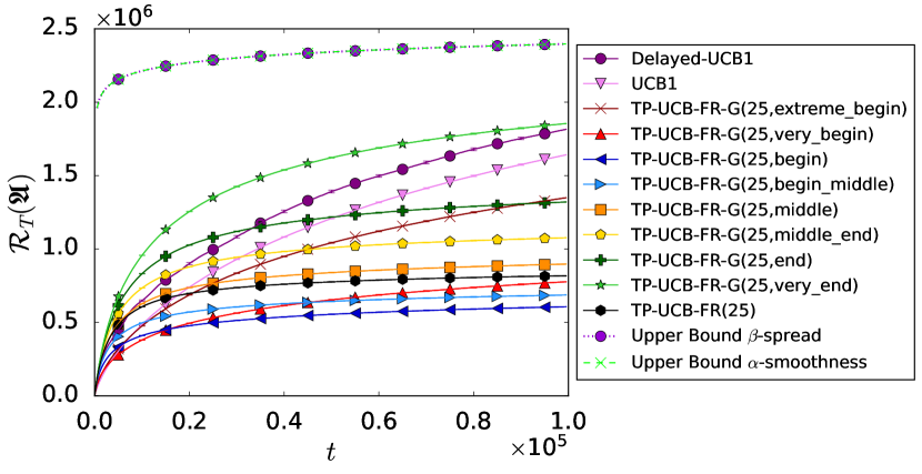
Figure 10: Regret against time for Setting 1 with $\alpha_{est}=25$

$\alpha$	Regret	Regret	$\delta^{+}$
	TP-UCB-FR	TP-UCB-FR-G	(%)
5	$1.34\times 10^{6}$	$1.28\times 10^{6}$	4.6*
10	$1.04\times 10^{6}$	$9.27\times 10^{5}$	10.9
20	$8.56\times 10^{5}$	$6.71\times 10^{5}$	21.6
25	$8.18\times 10^{5}$	$6.07\times 10^{5}$	25.8
50	$7.21\times 10^{5}$	$4.64\times 10^{5}$	35.6

Table 3: Summary of performance gains by TP-UCB-FR-G in Setting 1. *For $\alpha_{est}=5$ we show the begin_middle distribution as this is the only configuration where it performs better than the begin distribution implicitly assumed elsewhere.

In Table 3 we present a complete summary of the performance gains $\delta^{+}$ for Setting 1 using the begin distribution. Note that $\delta^{+}$ denotes the decrease of average regret in percentages with respect to the regret of TP-UCB-FR.

Setting 2

In the second setting, the effect of different (non-uniform) data generating distributions for the delayed partial rewards is evaluated. Furthermore, configurations with a higher $\tau_{\max}$ are tested. We model $K=10$ arms again with aggregate rewards after an arm pull s.t. $Z^{i}_{t,k}\sim\frac{\overline{R}^{i}}{\alpha}Beta(a^{i}_{k},b^{i}_{k})$. The time horizon is set to $T=10^{5}$. We evaluate four configurations and three scenarios. The four configurations are related to $\tau_{\max}$ and $\alpha$. The three scenarios differ from each other because of the distribution of partial rewards after an arm pull. The first scenario has a uniform aggregate reward distribution and is equal to Setting 1. The remaining two have higher rewards at the end of the $\tau_{\max}$ interval (Setting 2.1) and higher rewards just after the arm pull (Setting 2.2), respectively. The vectors $a^{i}$ and $b^{i}$ represent all values $a^{i}_{k}$ and $b^{i}_{k}$ for $k\in\{1,\dots,\alpha\}$ and can be found in the referenced tables 4, 5, 6 and 7.

• Configuration 1: $\tau_{\max}=100,\alpha=10$, see Table 4

• Configuration 2 $\tau_{\max}=100,\alpha=50$, see Table 5

• Configuration 3 $\tau_{\max}=200,\alpha=20$, see Table 6

• Configuration 4 $\tau_{\max}=200,\alpha=100$, see Table 7

Setting	Parameter vector
	$a^{i}$
Uniform	$\boldsymbol{1}_{\alpha}$
Setting 2.1	[2,4,6,8,10,10,10,10,10,10]
Setting 2.2	[10,10,10,10,10,10,8,6,4,2]
	$b^{i}$
Uniform	$\boldsymbol{1}_{\alpha}$
Setting 2.1	[10,10,10,10,10,10,8,6,4,2]
Setting 2.2	[2,4,6,8,10,10,10,10,10,10]

Table 4: Distribution parameters for different scenarios with Configuration 1

Setting	Parameter vector
	$a^{i}$
Uniform	$\boldsymbol{1}_{\alpha}$
Setting 2.1	[2,4, …, 48,50, …, 50]
Setting 2.2	[50, …, 50,48, …, 4,2]
	$b^{i}$
Uniform	$\boldsymbol{1}_{\alpha}$
Setting 2.1	[50, …, 50,48, …, 4,2]
Setting 2.2	[2,4, …, 48,50, …, 50]

Table 5: Distribution parameters for different scenarios with Configuration 2

Setting	Parameter vector
	$a^{i}$
Uniform	$\boldsymbol{1}_{\alpha}$
Setting 2.1	[2,4, …, 18,20, …, 20]
Setting 2.2	[20, …, 20,18, …, 4,2]
	$b^{i}$
Uniform	$\boldsymbol{1}_{\alpha}$
Setting 2.1	[20, …, 20,18, …, 4,2]
Setting 2.2	[2,4, …, 18,20, …, 20]

Table 6: Distribution parameters for different scenarios with Configuration 3

Setting	Parameter vector
	$a^{i}$
Uniform	$\boldsymbol{1}_{\alpha}$
Setting 2.1	[2,4, …, 98,100, …, 100]
Setting 2.2	[100, …, 100,98, …, 4,2]
	$b^{i}$
Uniform	$\boldsymbol{1}_{\alpha}$
Setting 2.1	[100, …, 100,98, …, 4,2]
Setting 2.2	[2,4, …, 98,100, …, 100]

Table 7: Distribution parameters for different scenarios with Configuration 4

Results

As discussed in the main paper in Section 6, the results for different scenarios within one configuration are visually indistinguishable. The analysis of Figure 3 in the same section shows that there are no significant differences between learner increases. It also shows that all learners perform best in Setting 2.2, worse in the uniform setting and worst in Setting 2.1. Because no visual distinction can be made, the results for Configuration 1 and Configuration 2 are visually identical to the results for Setting 1 with $\alpha_{est}=10$ and $\alpha_{est}=50$. Similarly, the results of the Setting 2 tests with uniform distribution are visually identical to the results of Setting 2.1 and 2.2. To show the change of our upper bound compared to the upper bound of TP-UCB-FR, we present the results of running Configuration 3 and 4 for Setting 2.1 and 2.2. The resulting plots can be seen in Figures 11, 12, 13 and 14. Furthermore, in Tables 8, 9 and 10, we provide a complete summary of the performance gains $\delta^{+}$ for different configurations in Setting 2 using the begin distribution.

Figure 11: Regret against time for Setting 2.1 with $\tau_{\max}=200,\alpha_{est}=20$

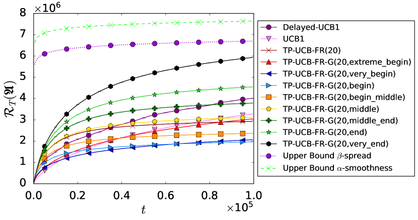
Figure 12: Regret against time for Setting 2.2 with $\tau_{\max}=200,\alpha_{est}=20$

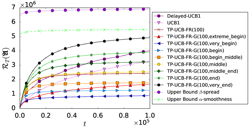
Figure 13: Regret against time for Setting 2.1 with $\tau_{\max}=200,\alpha_{est}=100$

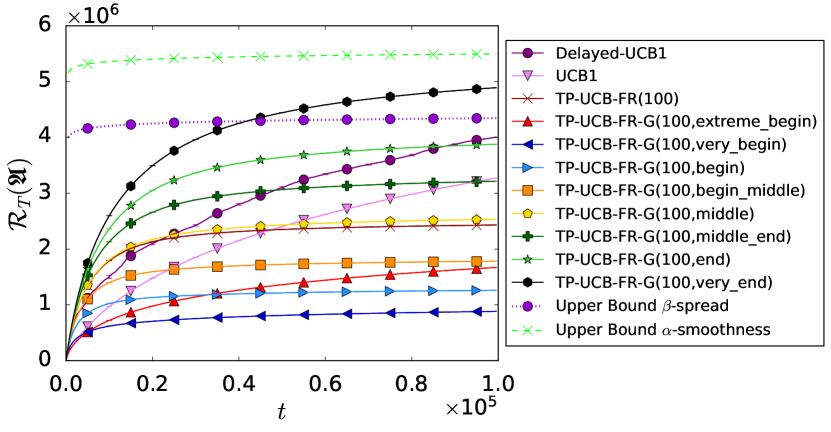
Figure 14: Regret against time for Setting 2.2 with $\tau_{\max}=200,\alpha_{est}=100$

$\tau_{\max}$	$\alpha$	Regret	Regret	$\delta^{+}$
		TP-UCB-FR	TP-UCB-FR-G	(%)
100	10	$1.04\times 10^{6}$	$9.27\times 10^{5}$	10.9
100	50	$7.19\times 10^{5}$	$4.66\times 10^{5}$	35.2
200	20	$2.94\times 10^{6}$	$1.98\times 10^{6}$	32.7
200	100	$2.45\times 10^{6}$	$1.27\times 10^{6}$	48.2

Table 8: Summary of performance gains $\delta^{+}$ by TP-UCB-FR-G in Setting 2.1

$\tau_{\max}$	$\alpha$	Regret	Regret	$\delta^{+}$
		TP-UCB-FR	TP-UCB-FR-G	(%)
100	10	$1.04\times 10^{6}$	$9.25\times 10^{5}$	11.0
100	50	$7.17\times 10^{5}$	$4.64\times 10^{5}$	35.3
200	20	$2.93\times 10^{6}$	$1.97\times 10^{6}$	32.8
200	100	$2.43\times 10^{6}$	$1.26\times 10^{6}$	48.1

Table 9: Summary of performance gains $\delta^{+}$ by TP-UCB-FR-G in Setting 2.2

$\tau_{\max}$	$\alpha$	Regret	Regret	$\delta^{+}$
		TP-UCB-FR	TP-UCB-FR-G	(%)
100	10	$1.04\times 10^{6}$	$9.28\times 10^{5}$	10.8
100	50	$7.18\times 10^{5}$	$4.65\times 10^{5}$	35.2
200	20	$2.94\times 10^{6}$	$1.98\times 10^{6}$	32.7
200	100	$2.44\times 10^{6}$	$1.27\times 10^{6}$	48.0

Table 10: Summary of performance gains $\delta^{+}$ by TP-UCB-FR-G in Setting 2 uniform

C.3.2 Spotify Setting

The Spotify setting is run with the same pre-processing and configuration detailed in Romano et al. [2022] to accurately compare the performance between their TP-UCB-FR algorithm and our proposed TP-UCB-FR-G algorithm. We average the results over 100 independent runs. The results of this setting can be seen in Figure 5.

C.4 Additional Experiments

C.4.1 Alternative distributions as input for TP-UCB-FR-G

In Section 6, we describe the results obtained by various settings, using Beta-Binomial distributions with different choices for their parameters. In general, the domain of a distribution must be bounded on the interval $[1,\alpha]$ in order to be used as input. Below, we describe several finite discrete distributions that can be restricted to have such a domain, and the outcomes of the experiments.

The Zipfian distribution

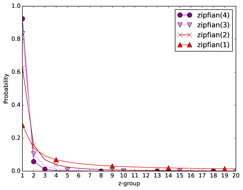
Figure 15: PMF of Zipfian distributions with different parameters

The Zipfian distribution allows us to describe ’begin-oriented’ distributions with different parameters, as seen in Figure 15. Since we observe that begin-oriented distributions pair well with our algorithm, Zipfian distributions should perform well in this setting.
Let us consider Setting 1. We run an experiment for $\alpha_{est}=20$, which is a perfect estimation of the smoothness factor. Furthermore, we only consider learners that are begin-oriented. We add 4 learners using Zipfian distributions with parameters $s\in[1,2,3,4]$ with names zipfian(1), zipfian(2), zipfian(3) and zipfian(4) respectively.

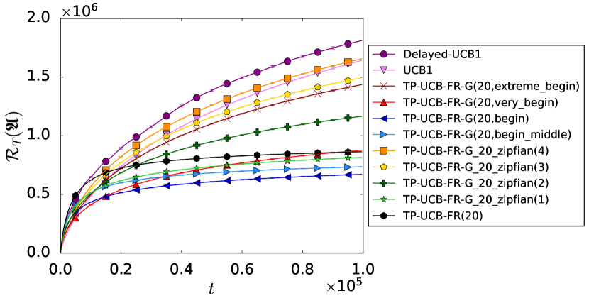
Figure 16: Zipfian and Beta-Binomial distribution comparison for Setting 1 with $\alpha_{est}=20$

We observe that the learner TP-UCB-FR-G_zipfian(1) performs better than the learner proposed by Romano et al. [2022], but worse than a begin-oriented Beta-Binomial learner. These results show that zipfian$(\zeta)$ learners for $\zeta\geq 2$ are outperformed by most Beta-Binomial learners, and do not bring any improvements to the results.

The Boltzmann distribution

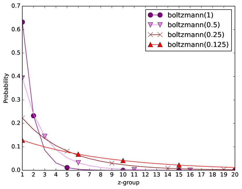
Figure 17: PMF of Boltzmann distributions with different parameters

In a similar way, we can also describe ’begin-oriented’ distributions using the Boltzmann distribution. We denote the input distribution as boltzmann$(\lambda)$. We notice that as $\lambda\to 0$, the distribution provides a smoother begin-orientation. This experiment is particularly interesting because for $\lambda=0.25$ and $\lambda=0.125$, the distribution is carefully begin-centered, so it could result in a performance gain. We consider again Setting 1. We run an experiment for $\alpha_{est}=20$, representing a perfect estimation of the smoothness factor. We consider the Beta-Binomial learners that are begin-oriented, and add Boltzmann distribution learners for $\lambda\in[1,0.5,0.25,0.125]$. The results for this experiment are shown in Figure 18.

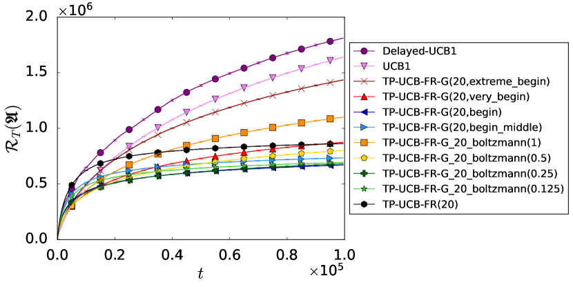
Figure 18: Boltzmann and Beta-Binomial distribution comparison for Setting 1 with $\alpha_{est}=20$

We observe that Boltzmann distributions, in particular Boltzmann(0.5), provide marginally better performance for $t=[0,15000]$, and is nearly identical to the curve of the very_begin learner. This is only logical, since the curves in Figures 6 and 17 are nearly identical. It is also important to observe that for $t=[0,38000]$, Boltzmann(0.25) provides marginally better performance than begin. For $t>38000$, begin is still the learner with the lowest regret. Since $\lambda=0.125$ starts to under-estimate, and $\lambda=1,\lambda=0.5$ are clear over-estimations, we have sufficient evidence that this distribution does not provide the required flexibility needed for performance gains over Beta-Binomial distributions. Precise regret values for this experiment, can be found in the supplementary material. We exclude extreme_begin and Boltzmann(1) because they are clear over-estimations, and Delayed-UCB, UCB because they are irrelevant for this comparison.

With the above results we conclude that Beta-Binomial distributions still give the best performance and flexibility, whilst Boltzmann distributions lack in both areas mentioned.

The Hypergeometric distribution
For a mathematical description of the Hypergeometric distribution, we refer to Lee [2012]. In short, a random variable $X$ follows a hypergeometric distribution if its probability mass function is defined as

$$p_{X}(k)=P(X=k)=\frac{\binom{K}{k}\binom{N-K}{n-k}}{\binom{N}{n}}$$ (17)

where $N$ is the population size, $K$ the number of success rates in the population, $n$ the number of draws and $k$ the number of successes for which the PMF returns the probability. We set $n$ and $K$ to $\alpha-1$, equal to the number of $z$-groups minus one and shift each value of $k$ given as input by 1 (similarly to our Beta-Binomial implementation), such that we bound $p_{X}(k)$ to the domain $[1,\alpha]$. We can then shape the distribution with some choice for $N\geq 2\alpha$. In this section, we denote learners using the Hypergeometric distribution as Hypergeom(N) where the shaping parameter $N\in\mathbb{N}$ and $N\geq 2\alpha=40$. We shall describe several begin-oriented hypergeometric distributions for $N\in[50,100,200,300,400,500]$. Figure 19 depicts the corresponding probability mass functions for $N$.

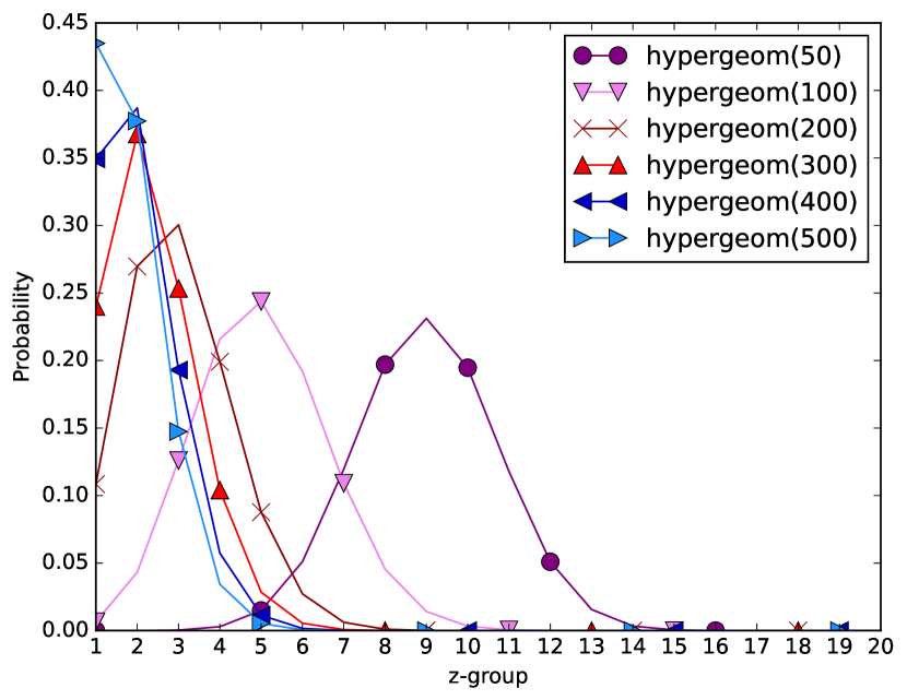
Figure 19: PMF of Hypergeometric distributions with different parameters

We shall include begin-oriented beta-binomial learners for comparison, and run Setting 1 with $\alpha_{est}=20$, a perfect smoothness factor estimation. The results for this experiment are shown in Figure 20

Figure 20: Hypergeometric and Beta-Binomial distribution comparison for Setting 1 with $\alpha_{est}=20$

Again, we observe that TP-UCB-FR-G$(20,\texttt{begin})$ is the best performing learner when averaged over the entire time horizon $T$. However, for $t\in[0,15000]$, hypergeom$(N)$ with $N\in[200,300,400,500]$, learners with such distributions perform marginally better. Due to the slope of the corresponding curves created by hypergeometric distributions, their performance degrades as $t$ gets larger. Due to the large gaps between $N$, one could search for the most appropriate value for $N$ and perhaps discover a distribution that performs better than the begin Beta-Binomial learner, but this requires running Setting 1 for $200\leq N\leq 500$ which is very costly. Moreover, we could fine-tune the Beta-Binomial learner in a similar way, by running Setting 1 for different $\alpha,\beta$ in the proximity of begin, which will result in far less runs. Again, the Beta-Binomial distribution remains superior in flexibility and performance.

C.4.2 Relation between assumed distribution and upper bound

As mentioned in Theorem 2, the upper bound on TP-UCB-FR-G learners only holds when the assumed distribution that is given as input to the algorithm matches the data generating distribution. In this section, we want to go into more detail about this and discuss which type of learner, with a non-matching assumed distribution, stays below this upper bound.

We note that this phenomenon, although not mentioned explicitly in Romano et al. [2022], is also present for the upper bound of the TP-UCB-FR algorithm and that it depends on the $\alpha$ of the data generating distribution and not on the estimate given as input. Because the assumed distribution for this algorithm is univariate (only depending on $\alpha$), determining which learners do not exceed the upper bound is tested more easily: an increased $\alpha_{est}$ always leads to better results in all tested settings (see section 6). This means that learners typically stay below the upper bound when $\alpha_{est}\in[\alpha,\tau_{\max}]$.

However, the upper bound of TP-UCB-FR-G depends on three properties of the data generating distribution, namely its expected value, the index of coincidence and $\alpha$. In the results (see section 6), we see that learners with a lower assumed expected value generally perform better. But there is a limit to how low the expected value can be, because the second factor, the index of coincidence, gets relatively high for very begin oriented distributions which raises the regret. This makes it harder to give an empirical estimate about which kind of learners stay below the theoretical upper bound. It also shows that learners with a higher $\alpha$ perform better, similarly to the case of TP-UCB-FR. Deriving the precise correlation between these three parameters is highly complex and it is a potential future work.

References

- Agarwal and Duchi [2011] Alekh Agarwal and John C Duchi. Distributed delayed stochastic optimization. In Advances in Neural Information Processing Systems, volume 24, 2011.
- Arya and Yang [2020] Sakshi Arya and Yuhong Yang. Randomized allocation with nonparametric estimation for contextual multi-armed bandits with delayed rewards. Statistics & Probability Letters, 164:108818, 2020.
- Auer et al. [2002] Peter Auer, Nicolò Cesa-Bianchi, and Paul Fischer. Finite-time analysis of the multiarmed bandit problem. Machine Learning 2002 47:2, 47:235–256, 5 2002.
- Brost et al. [2019] Brian Brost, Rishabh Mehrotra, and Tristan Jehan. The music streaming sessions dataset. CoRR, abs/1901.09851, 2019.
- Bubeck and Cesa-Bianchi [2012a] Sébastien Bubeck and Nicolò Cesa-Bianchi. Regret analysis of stochastic and nonstochastic multi-armed bandit problems. Foundations and Trends in Machine Learning, 5(1):1–122, 2012.
- Bubeck and Cesa-Bianchi [2012b] Sébastien Bubeck and Nicolò Cesa-Bianchi. Regret analysis of stochastic and nonstochastic multi-armed bandit problems. CoRR, abs/1204.5721, 2012.
- Cesa-Bianchi et al. [2022] Nicolò Cesa-Bianchi, Tommaso Cesari, Roberto Colomboni, Claudio Gentile, and Yishay Mansour. Nonstochastic bandits with composite anonymous feedback. Journal of Machine Learning Research, 23(277):1–24, 2022.
- Desautels et al. [2014] Thomas Desautels, Andreas Krause, and Joel W. Burdick. Parallelizing exploration-exploitation tradeoffs in gaussian process bandit optimization. The Journal of Machine Learning Reseacrh, 15(1):3873–3923, jan 2014.
- Friedman [1987] William Frederick Friedman. The index of coincidence and its applications in cryptanalysis, volume 49. Aegean Park Press California, 1987.
- Gael et al. [2020] Manegueu Anne Gael, Claire Vernade, Alexandra Carpentier, and Michal Valko. Stochastic bandits with arm-dependent delays. In Proceedings of the 37th International Conference on Machine Learning, volume 119 of Proceedings of Machine Learning Research, pages 3348–3356, 13–18 Jul 2020.
- Hoeffding [1963] Wassily Hoeffding. Probability inequalities for sums of bounded random variables. Journal of the American Statistical Association, 58(301):13–30, 1963.
- Joulani et al. [2013] Pooria Joulani, András György, and Csaba Szepesvári. Online learning under delayed feedback. In Proceedings of the 30th International Conference on International Conference on Machine Learning - Volume 28, ICML’13, 2013.
- Lai and Robbins [1985] T.L Lai and Herbert Robbins. Asymptotically efficient adaptive allocation rules. Advances in Applied Mathematics, 6(1):4–22, 1985.
- Lee [2012] Peter M. Lee. 3.1 The binomial distribution. Wiley, 4 edition, 2012.
- Mandel et al. [2015] Travis Mandel, Yun-En Liu, Emma Brunskill, and Zoran Popović. The queue method: Handling delay, heuristics, prior data, and evaluation in bandits. In Twenty-Ninth AAAI Conference on Artificial Intelligence, 2015.
- Mesterharm [2005] Chris Mesterharm. On-line learning with delayed label feedback. In Proceedings of the 16th International Conference on Algorithmic Learning Theory, page 399–413, 2005.
- Mesterharm [2007] Chris Mesterharm. Improving on-line learning. PhD thesis, Rutgers University, 2007.
- Pandey et al. [2007] Sandeep Pandey, Deepayan Chakrabarti, and Deepak Agarwal. Multi-armed bandit problems with dependent arms. In Proceedings of the 24th international conference on Machine learning, pages 721–728, 2007.
- Pike-Burke et al. [2018] Ciara Pike-Burke, Shipra Agrawal, Csaba Szepesvari, and Steffen Grunewalder. Bandits with delayed, aggregated anonymous feedback. In International Conference on Machine Learning, pages 4105–4113. PMLR, 2018.
- Romano et al. [2022] Giulia Romano, Andrea Agostini, Francesco Trovò, Nicola Gatti, and Marcello Restelli. Multi-armed bandit problem with temporally-partitioned rewards: When partial feedback counts. Proceedings of the Thirty-First International Joint Conference on Artificial Intelligence, 2022.
- Vernade et al. [2017] Claire Vernade, Olivier Cappé, and Vianney Perchet. Stochastic Bandit Models for Delayed Conversions. In Conference on Uncertainty in Artificial Intelligence, Sydney, Australia, August 2017.
- Vernade et al. [2020a] Claire Vernade, Alexandra Carpentier, Tor Lattimore, Giovanni Zappella, Beyza Ermis, and Michael Brückner. Linear bandits with stochastic delayed feedback. In Proceedings of the 37th International Conference on Machine Learning, volume 119 of Proceedings of Machine Learning Research, pages 9712–9721, 13–18 Jul 2020.
- Vernade et al. [2020b] Claire Vernade, András György, and Timothy A. Mann. Non-stationary delayed bandits with intermediate observations. In Proceedings of the 37th International Conference on Machine Learning, ICML’20, 2020.
- Wang et al. [2021] Siwei Wang, Haoyun Wang, and Longbo Huang. Adaptive algorithms for multi-armed bandit with composite and anonymous feedback. Proceedings of the AAAI Conference on Artificial Intelligence, 35(11):10210–10217, 2021.
- Weinberger and Ordentlich [2002] M.J. Weinberger and E. Ordentlich. On delayed prediction of individual sequences. IEEE Transactions on Information Theory, 48(7):1959–1976, 2002.
- Zhou et al. [2019] Zhengyuan Zhou, Renyuan Xu, and Jose Blanchet4. Learning in Generalized Linear Contextual Bandits with Stochastic Delays. Curran Associates Inc., 2019.
- Zinkevich et al. [2009] Martin Zinkevich, John Langford, and Alex Smola. Slow learners are fast. In Advances in Neural Information Processing Systems, volume 22, 2009.