A Hybrid Genetic Algorithm with Type-Aware Chromosomes for Traveling Salesman Problems with Drone

Abstract

There are emerging transportation problems known as the Traveling Salesman Problem with Drone (TSPD) and the Flying Sidekick Traveling Salesman Problem (FSTSP) that involve the use of a drone in conjunction with a truck for package delivery. This study represents a hybrid genetic algorithm for solving TSPD and FSTSP by combining local search methods and dynamic programming. Similar algorithms exist in the literature. Our algorithm, however, considers more sophisticated chromosomes and simpler dynamic programming to enable broader exploration by the genetic algorithm and efficient exploitation through dynamic programming and local searches. The key contribution of this paper is the discovery of how decision-making processes should be divided among the layers of genetic algorithm, dynamic programming, and local search. In particular, our genetic algorithm generates the truck and the drone sequences separately and encodes them in a type-aware chromosome, wherein each customer is assigned to either the truck or the drone. We apply local searches to each chromosome, which is decoded by dynamic programming for fitness evaluation. Our dynamic programming algorithm merges the two sequences by determining optimal launch and landing locations for the drone to construct a TSPD solution represented by the chromosome. We propose novel type-aware order crossover operations and effective local search methods. A strategy to escape from local optima is proposed. Our new algorithm is shown to outperform existing algorithms on most benchmark instances in both quality and time. Our algorithms found the new best solutions for 538 TSPD instances out of 920 and 93 FSTSP instances out of 132.

Keywords:

vehicle routing; traveling salesman problem; genetic algorithm; dynamic programming

1 Introduction

With the growing number of online orders, companies are competing to ship products in a timely manner. This underscores the need for improved delivery methods. Traditional methods include using the Traveling Salesman Problem (TSP), in which a vehicle, perhaps a truck, takes multiple orders and delivers them to customers as soon as possible. As a result of the truck’s low speed and need to maneuver around traffic flows, many big companies such as Amazon and UPS are looking for new delivery methods like drones. Unlike traditional trucks, drones do not have to follow the same network, giving them faster delivery times. They are also more eco-friendly since they are electrical and less expensive since they do not require any human involvement.

It is important to note that drones also come with some significant limitations. Unlike trucks, these do not have the capability of carrying heavy or multiple parcels. To be able to pick up an item after every delivery, a drone must return to the warehouse. Drones are limited in their range because of their battery capacity and cannot reach remote customers.

Recent efforts have been made to utilize the advantages of both vehicles and include a delivery method in which the truck and the drone collaborate. Murray and Chu (2015) described the combined problem as the Flying Sidekick Traveling Salesman Problem (FSTSP), in which a drone lies on top of a truck and can fly at various points, deliver a parcel to a customer, and land on the truck at another point while the truck can make deliveries at the same time. A similar problem was later introduced by Agatz et al. (2018) as the Traveling Salesman Problem with Drone (TSPD) with slightly simpler assumptions. We will discuss the differences between the two problems in Section 3. We refer readers to Chung et al. (2020) and Macrina et al. (2020) for other problems that involve both ground vehicles and drones.

A hybrid genetic algorithm (HGA) is presented in this study for solving both TSPD and FSTSP with the aim of minimizing total delivery time. While regular genetic algorithms only rely on crossovers and mutations to generate new solutions, hybrid genetic algorithms usually improve the generated solutions by local search methods or other heuristics in addition to those conventional techniques. Hybrid genetic algorithms have been actively developed to solve various vehicle routing problems (Ho et al., 2008; Vidal et al., 2012), including the problem of our interest, TSPD/FSTSP (Ha et al., 2020).

Our HGA approach consists of three layers in its algorithmic structure. First, a regular genetic algorithm (GA) layer generates incomplete solutions by determining the customer nodes served by the truck and the drone, called truck nodes and drone nodes, respectively. Second, a dynamic programming (DP) layer completes the solutions by determining the combined nodes, where the drone departs from the truck or returns to the truck. Third, we use various local searches to improve the generated solutions.

The key contribution of this paper is the discovery of how decision-making processes should be divided among these three layers. Similar approaches exist in the literature, especially, Ha et al. (2020), whose GA layer is simple while the difficult decision-making step is handled by their DP layer. We give more informed exploratory roles in the GA layer, while we use a much simpler DP layer so that the decoding and evaluation for exploitation are faster. Our GA layer utilizes a novel type-aware chromosome (TAC) encoding to distinguish truck and drone nodes. We also devise type-aware order crossover operations to support the TAC encoding in the GA layer. Our unique TAC encoding makes the time complexity of the DP layer less than other DP-based approaches used in the literature. With the TAC encoding, it is easy to devise various local search schemes directly on the chromosomes, it is unnecessary to apply additional encoding on the decoded solutions from the DP layer, and it is possible to keep high-resolution information on the solutions in the GA populations. Furthermore, our GA layer uses two or three subpopulations, depending on whether the drone range is limited, and we propose an escaping strategy for preventing GAs from being trapped in local optima. The proposed division of three layers with the TAC encoding brings the reduction in the objective function values, the savings in the computational time, or both, in most benchmark instances.

The remainder of the paper is organized as follows. A brief summary of the literature is given in Section 2, and a formal definition of the problem is given in Section 3. The methodology is described in Section 4, and the numerical results from the experiments are given in Section 5. Finally, the conclusion and future directions are discussed in Section 6. In the rest of the paper, we call our method the HGA with TAC, or HGA-TAC, to emphasize the significance of the TAC encoding.

2 Literature Review

The number of recent publications that are dedicated to the study of last-mile delivery with truck and drone collaboration is rapidly increasing, and because of this, the majority of the articles that we review are those that are pertinent to our work. We refer to survey papers, Otto et al. (2018), Macrina et al. (2020), and Chung et al. (2020), for general overviews on the optimization of problems with various applications of drones. Several approaches have been taken in the literature to study the collaboration between trucks and drones. Note that the research topics differ regarding the number of vehicles, the basic assumptions and limitations, and the method of solving them. As this study focuses on the collaboration between a single truck and a single drone with only one visit per flight, we review the most relevant papers in this section; however, we briefly mention some other variants of the problem.

We begin by reviewing the papers that first proposed the problem. Our next step is to review publications that employ heuristic approaches, followed by those that utilize exact approaches. Then we briefly introduce two papers that use machine learning techniques to solve the problem. Last but not least, we discuss some of the articles that deal with extensions of the problem.

Murray and Chu (2015) introduced the FSTSP for the first time with a mixed-integer linear programming (MILP) formulation and a heuristic algorithm. Later, Agatz et al. (2018) studied a slightly different problem, defined as the TSPD. The main difference is that the drone can wait for the truck in the TSPD but not in the FSTSP, among other differences in the assumptions. To solve the TSPD, they proposed an MILP formulation, which is computationally tractable for small problems with up to twelve customers. They provide a heuristic algorithm, called ‘TSP-ep-all’, that combines neighborhood search and a partitioning algorithm, which begins with an optimal or near-optimal TSP tour. Given the initial TSP tour, they use a dynamic programming (DP) approach to determine which customers should be visited by the drone, while maintaining the order in the given TSP tour. This procedure is called the exact partitioning of customers. Then the TSP-ep-all algorithm generates other TSP tours by perturbing the TSP tour using local search methods such as the two-opt swap, the three-opt swap, and the two-point swap, which are popularly used in TSP heuristics. For each generated TSP tour, the exact partitioning is used to create a TSPD solution. The algorithm returns the minimal delivery time TSPD solution as the final solution. This method has been shown efficient and effective in small to medium size problems with less than 50 customers, but it shows exponentially increasing computational time due to the extensive local searches on the initial TSP tour. They also created a benchmark TSPD dataset, which we will use to compare our algorithm with other methods.

Various metaheuristic methods have been developed successfully in the literature. Most related to our approach are the Hybrid General Variable Neighborhood Search (HGVNS) of de Freitas and Penna (2020) and the Hybrid Genetic Algorithm (HGA20) of Ha et al. (2020); not to be confused with our HGA approach, we use the acronym ‘HGA20’ for the method of Ha et al. (2020) throughout the paper. HGVNS also starts with an optimal or near-optimal TSP solution, then converts it to an initial solution by creating sub-routes for the drone. Finally, HGVNS improves the solution by a variable neighborhood search. HGA20 represents each chromosome in the form of a giant tour that corresponds to the TSP tour. The Split method, a polynomial time algorithm proposed in Ha et al. (2018), is employed at each step in order to convert the giant tour chromosome into the FSTSP tour. Then, local search methods are applied for improvement, and finally, using a restore method, the improved FSTSP tour is converted back into the giant tour chromosome. The chromosome encoding in our approach, however, includes the truck sequence as well as the drone sequence. Only the locations of drone launches and landings remain, which are determined by dynamic programming in an optimal manner.

(a) TSP-ep-all

(b) HGA20

(c) HGA-TAC in this paper

Figure 1: Comparing the structure of our approach to TSP-ep-all in Agatz et al. (2018) and HGA20 in Ha et al. (2020)

Figure 1 provides an overview of our algorithm’s structure so that it can be compared to TSP-ep-all and HGA20. Observably, TSP-ep-all takes a TSP tour and applies exact partitioning, or Partition, to transform it optimally to a TSPD solution with a time complexity of $O(n^{3})$, $n$ being the number of customer nodes. In HGA20, multiple TSP tours are generated by crossover within GA, and the TSPD solution is obtained using the Split method with a time complexity of $O(n^{4})$, which is analogous to Partition. Then the TSPD solution is restored as a chromosome (TSP tour) and reintroduced to the GA population pool.

In our methodology, each chromosome is designed to store more information. GA also determines the vehicle type used to serve each customer, in addition to the order. As illustrated in Figure 1(c), each chromosome consists of a sequence of numbers which represent the customers. The positive and negative numbers indicate the customers that will be visited by truck and drone, respectively. To achieve the TSPD solution, it is sufficient to establish where the drone is released from and returns to the truck. To discover the rendezvous points optimally, we devise a dynamic programming algorithm, Join, with the time complexity of $O(n^{2})$. To summarize, the type of vehicle required for each node is decided in Partition and Split, in addition to rendezvous points, while in our Join approach, the first decision has been assigned to GA.

There is another point of comparison that can be drawn between these three approaches: local searches. The TSP-ep-all algorithm executes local searches on TSP tours before applying Partition, while the HGA20 algorithm performs local searches after applying Split on TSPD solutions before converting back to chromosomes. This paper uses local searches inspired by TSPD directly on the chromosome before Join is applied; hence no additional encoding is necessary. Besides the faster decoding algorithm, this is another advantage of our method.

Other metaheuristic methods for TSPD/FSTSP include a greedy randomized adaptive search procedure (Ha et al., 2018), a multi-start variable neighborhood search (Campuzano et al., 2021), and a multi-start tabu search (Luo et al., 2021).

Numerous studies have attempted to solve TSPD using exact methods. A dynamic programming approach was developed by Bouman et al. (2018) in order to find an optimal solution to TSPD. They were able to solve the problem with up to 20 customers using their DP. The branch-and-bound algorithm proposed by Poikonen et al. (2019) is also capable of solving TSPD up to 20 nodes at optimum. Additionally, they devised a divide-and-conquer heuristic based on their branch-and-bound algorithm that delivers high-quality solutions. Boccia et al. (2021) introduces a new representation of the FSTSP based on the definition of an extended graph. They presented a new MILP formulation and a branch-and-cut algorithm for solving the problem, which was able to find optimal solutions for problems with up to 20 customers. Roberti and Ruthmair (2021) creates a new MILP that is more effective and able to accommodate a variety of side constraints. They propose a branch-and-price approach wherein they establish a set partitioning problem and then use the ng-route relaxation to formulate the pricing problem. Their technique optimally solves TSPD instances for problems with up to 39 customers.

The use of learning-based methods has been reported in a few papers that address TSPD. The K-Means Clustering algorithm is employed by Ferrandez et al. (2016) to determine launch locations, and the Genetic Algorithm is used to solve a TSP and determine the truck routes. As part of their objective function, they also aim to minimize the amount of energy consumed as well as the delivery time. The study also examined the case of multiple drones per truck. Bogyrbayeva et al. (2023) designs and trains a deep reinforcement learning algorithm for solving TSPD and examines it on instances with up to 100 nodes in size. Aside from the training time, their algorithm is capable of solving instances within a relatively short period of time.

There have been several extensions to TSPD, and FSTSP introduced and studied in the literature. Murray and Raj (2020) proposes mFSTSP in which the truck can collaborate with multiple drones in order to deliver parcels. As part of their work, they develop an MILP formulation as well as a heuristic algorithm for solving the problem. Gonzalez-R et al. (2020) also proposes that the drone can visit multiple customers during the course of each trip as a generalization of the FSTSP. This problem is referred to as truck-drone team logistics (TDTL), an MILP formulation is presented, and an iterated greedy approach is applied to solve it.

Most studies have focused either on TSPD or FSTSP, with a few exceptions, such as de Freitas and Penna (2020), which is implemented in both problem settings. It is also important to note that the existing algorithms for TSPD are not exempt from the trade-off rule between solution quality and running time. This work aims to solve both problems, with a particular focus on the disparities in underlying assumptions, and testing on a range of instances from the literature reveals that our method can provide viable solutions in a reasonable amount of time.

(a) The minimum time solved by TSP is 39

(b) The minimum time by TSPD is 25

Figure 2: A network with one depot and 5 customers solved by TSP and TSPD.

3 Problem Statement

In this section, we introduce TSPD and FSTSP formally and describe their associated assumptions. As explained before, the TSPD system involves coordinating a truck with a drone to deliver goods. As the drone resides on the truck’s roof, it can be launched to deliver a package to a customer and then returned to the top of the truck. The TSPD can be represented in a graph $G(\mathcal{V},\mathcal{E})$ where $\mathcal{V}=\{0,1,...,n\}$ is the set of nodes and $\mathcal{E}$ is the set of edges in the graph which is assumed to be complete. We let $N=|\mathcal{V}|=n+1$. Vehicles start their routes at the depot node $0$ and must return to it after completing their deliveries; for returning, the depot is represented as $0^{\prime}$. The remaining nodes refer to the locations of customers. The travel time between the nodes may vary in accordance with the type of vehicle and the assumptions made about the problem. The ratio of drone speed to truck speed is represented by $\alpha$. For instance, if $\alpha=2$ and the distance is determined using the same metrics, the travel time for a drone between two geographical locations will be half of the time required for a truck to travel between the same nodes.

Before delving into the specifics, it would be extremely helpful to see an example of a simple network solved with TSPD and the amount of time saved over regular TSP. Figure 2(a) depicts the optimal TSP solution for a network with one depot and five customers, whereas Figure 2(b) illustrates the same network utilizing a truck and a drone in collaboration. Numbers on the arcs indicate traversal times for corresponding vehicles with $\alpha=2$. The set of deliveries made by the cooperation of two vehicles between each launch and land is named an operation by Agatz et al. (2018) and sortie by Murray and Chu (2015). Each operation is defined as $\langle i,j,k\rangle$, where $i$ is the position where the drone launches, $j$ is the location where the customer is served, and $k$ is the position where the drone lands on the truck. In the first operation $\langle 0,1,2\rangle$, for instance, the drone takes off from the depot, makes a delivery to the customer at node 1, and lands on the truck at node 2. The minimum time for each operation can be calculated as $\max\{\tau_{i\rightarrow k}^{\mathrm{tr}},\tau_{i,j}^{\mathrm{dr}}+\tau_{j,k}^{\mathrm{dr}}\}$ where $\tau_{i\rightarrow k}^{\mathrm{tr}}$ is truck’s travel time from $i$ to $k$ traversing all the nodes in between if any, and $\tau_{i,j}^{\mathrm{dr}}$ is drone’s travel time between two nodes. In this simplified instance, TSPD shows a 36 percent improvement over TSP, which indicates that drones can serve a valuable and beneficial function for last-mile delivery.

We first state the common assumptions of the TSPD and FSTSP, and then problem-specific assumptions.

3.1 Common Assumptions

Both TSPD and FSTSP make the following assumptions:

1. Both vehicles start their tour at the depot and must return there at the end of their tour after completing all deliveries.

2. In each operation, the drone is only permitted to visit one customer before returning to either the truck or depot. While the drone is in flight, the truck can make multiple deliveries.

3. Drone launches only at customer locations or depot $0$ and lands only at customer locations or depot $0^{\prime}$.

4. Each customer is visited only once by either the drone or the truck. While customers are served by the truck, the drone might be onboard with the truck or in flight.

3.2 Problem-Specific Assumptions

All of the above general assumptions hold true for both TSPD and FSTSP, whereas the specific assumptions for each problem are listed below.

1. Launch and landing nodes: In both cases, the drone can be relaunched from the same spot on the vehicle where it landed. However, in FSTSP, drones cannot land on the same node from where they are launched, but in TSPD, this is permitted.

2. Setup times: TSPD disregards pickup time, delivery time, and recharging (battery changing) time, whereas FSTSP includes preparation time denoted $s_{L}$ before a launch for changing the battery and loading the cargo, and retrieval time when landing on the truck denoted $s_{R}$.

3. Drone eligible nodes: In TSPD, all customers can be visited and serviced by either vehicle; however, in FSTSP, some customers cannot be visited by drone for a variety of reasons. It could be due to a heavy package that cannot be carried by a drone, the necessity for a signature, or an impractical landing site.

4. Flying range: The drone has a limited flight time due to its limited battery capacity. Agatz et al. (2018) resolves the problem under both the premise of limitless and limited flight endurance. In TSPD, the flying range constraint just contains the time that a drone flies between nodes, whereas in FSTSP, it also includes the time that the drone must remain in constant flight if waiting for the truck at the rendezvous point, as it is not permitted to land and wait for the truck. For the same reason, each FSTSP operation must adhere to the same flying endurance constraint for the truck. For clarity, let $e$ represent the drone’s endurance. For operation $\langle i,j,k\rangle$, the relevant TSPD constraint for the drone solely is:

   $$\tau_{i,j}^{\mathrm{dr}}+\tau_{j,k}^{\mathrm{dr}}\leq e.$$

   While in the case of FSTSP, the constraint for drone is:

   $$\tau_{i,j}^{\mathrm{dr}}+\tau_{j,k}^{\mathrm{dr}}+s_{R}\leq e.$$

   For the truck, it is:

   $$\tau_{i\rightarrow k}^{\mathrm{tr}}+s_{T}\leq e,$$

   where $\tau_{i\rightarrow k}^{\mathrm{tr}}$ is the truck’s travel time from $i$ to $k$ while making deliveries in between, and $s_{T}$ is the service time. If the drone is being re-launched at node $k$, then $s_{T}=s_{R}+s_{L}$, and $s_{T}=s_{R}$ otherwise.

Despite the fact that these problem names have been used interchangeably in the literature, or some studies may include a combination of these assumptions, we tried to categorize the assumptions based on the first two papers that introduced the problem. In this study, we address both of these problems in our algorithm and solve instances from both natures and compare our results with the best current methods. These differences in the problem assumptions are handled mainly in the dynamic programming layer.

4 A Hybrid Genetic Algorithm with Type-Aware Chromosomes

In this section, we will describe the structure of our genetic algorithm, provide the local search methods, expound on our dynamic programming technique, and introduce our strategy for escaping local optima.

The algorithm we propose is a hybrid genetic algorithm (HGA) similar to Vidal et al. (2012) in terms of its basic construction. We search for both feasible and infeasible solutions stored in two sub-populations. Additionally, we take advantage of the contribution each individual provides to the diversity of the gene pool rather than only considering the cost of the solution. Ha et al. (2020) also employs this structure for solving FSTSP but uses a completely different representation of solutions and fitness evaluation technique from ours, as explained in Section 2.

Algorithm 1 displays our HGA’s general structure. Beginning with an initial population (Lines 1-3), two parents are chosen at random from the entire population (Line 5), one offspring is produced by a crossover between the two selected parents, and a modest probability of mutation is then applied to the offspring (Lines 6 and 7). Then, in order to raise the caliber of the solutions, local search techniques are applied to the offspring (Line 8). A feasibility assessment is conducted, and the offspring is added to the corresponding subpopulation. The infeasible offspring, however, is repaired and added to the feasible subpopulation with a specific probability (Lines 9-19). By picking survivors and adjusting penalties, the population size is managed (Lines 20-23). In the event that the solution does not improve after a certain number of iterations, we either try to diversify the population or escape the local optima, which will be discussed in greater detail (Lines 24-29).

The remaining portion of this section is summarized as follows: In Section 4.1, solution representation is explained, followed by the generation of the initial population in Section 4.2. Then our dynamic programming algorithm, Join, designed for an individual evaluation, is proposed in Section 4.3. Our next steps include parent selection, crossover, and mutation in Section 4.4, as well as local search and population management in Section 4.5 and 4.6, respectively. Finally, we explain our escaping strategy in Section 4.7.

Algorithm 1 Hybrid Genetic Algorithm with Type-Aware Chromosomes

1:$\Omega_{\textsc{f}}\leftarrow\emptyset$ $\triangleright$ Feasible population

2:$\Omega_{\textsc{inf}}\leftarrow\emptyset$ $\triangleright$ Infeasible population

3:$\Omega_{\textsc{f}},\Omega_{\textsc{inf}}=\texttt{initial\_population()}$ $\triangleright$ Algorithm 2

4:while number of iterations with no improvement $<It_{\textsc{NI}}$ do

5:     Select $\omega_{1}$ and $\omega_{2}$ from $\Omega_{\textsc{f}}\cup\Omega_{\textsc{inf}}$

6:     $\omega\leftarrow\texttt{crossover}(\omega_{1},\omega_{2})$

7:     $\texttt{mutate}(\omega)$

8:     $\texttt{local\_search}(\omega)$

9:     if $\omega$ is feasible then

10:         $\Omega_{\textsc{f}}\leftarrow\Omega_{\textsc{f}}\cup\{\omega\}$

11:     else

12:         $r\leftarrow\texttt{rand}(0,1)$

13:         if $r<P_{\textsc{REPAIR}}$ then

14:              Make $\omega$ feasible

15:              $\Omega_{\textsc{f}}\leftarrow\Omega_{\textsc{f}}\cup\{\omega\}$

16:         else

17:              $\Omega_{\textsc{inf}}\leftarrow\Omega_{\textsc{inf}}\cup\{\omega\}$

18:         end if

19:     end if

20:     if  $\texttt{size}(\Omega_{\textsc{f(inf)}})=\mu+\lambda$ then

21:         $\texttt{select\_survivors}(\Omega_{\textsc{f(inf)}})$

22:     end if

23:     Adjust penalties

24:     if $\texttt{best}(\Omega_{\textsc{f}})$ not improved for $It_{\textsc{DIV}}$ iterations then

25:         $\texttt{diversify}(\Omega_{\textsc{f}},\Omega_{\textsc{inf}})$

26:     end if

27:     if $\texttt{best}(\Omega_{\textsc{f}})$ not improved for $It_{\textsc{LOC}}$ iterations then

28:         $\texttt{escape\_local\_optima}(\texttt{best}(\Omega_{\textsc{f}}))$. $\triangleright$ Algorithm 3

29:     end if

30:end while

31:Return $\texttt{best}(\Omega_{\textsc{f}})$

4.1 Type-Aware Chromosome Encoding

The route taken by each vehicle, as well as the locations where the drone is launched from and lands on the truck, are the answers to the TSPD and the FSTSP. Our HGA for TSPD/FSTSP is unique in how we encode each solution in a chromosome, which keeps a sequence of customer nodes and records the type of each node: either a truck node or a drone node. Hence, we call our HGA the HGA with Type-Aware Chromosomes (HGA-TAC). While each number in HGA-TAC’s Chromosome encoding represents a customer node in the sequence, the truck nodes are represented by positive numbers, and the drone nodes are shown by negative numbers. Therefore, each chromosome includes the truck route as well as the drone route, and the TSPD/FSTSP tour will be accomplished if the launch and landing points are known. To handle such type-aware chromosomes, we devise a novel dynamic programming formulation and type-aware crossover operations. The proposed dynamic programming method, which we call Join, determines the optimal launch and landing points for the drone. The details of the Join algorithm will be discussed in 4.3.

A simple example will serve as a better understanding of our chromosome encoding. Consider a network that has ten customers. Figure 3(a) illustrates how the chromosome of an individual is coded in our algorithm before and after the addition of the depot. As mentioned previously, positive and negative numbers represent the nodes visited by truck and drone, respectively. The truck tour in this example is $[0-4-6-9-3-1-10-0^{\prime}]$, while the drone tour is $[0-2-5-8-7-0^{\prime}]$. The TSPD solution is shown in Figure 3(b) if we assume the launch and landing locations found by Join are $\{0,6,3,10\}$ and $\{6,3,1,0^{\prime}\}$ respectively.

4.2 Generating Initial Subpopulations

In the case that the drone is limited to only one customer per flight, any two or more consecutive negative numbers would be considered infeasible in our chromosome encoding. Additionally, if the drone’s flight range is restricted, a representation can be evaluated for feasibility. Therefore, our GA will have two sub-populations when the drone range is unlimited and three sub-populations otherwise. There is evidence in the literature that using infeasible solutions can significantly improve algorithm performance. As shown in Glover and Hao (2011), strategic oscillations between feasible and infeasible spaces are able to overcome some of the limitations associated with the metaheuristic methods. Using two or three types of subpopulations in this study, we take advantage of the diversity caused by the oscillations.

Algorithm 2 illustrates how the initial population is generated. Initially, we find a TSP solution, then promote it to a TSPD solution using the exact partitioning proposed in Agatz et al. (2018). The initial TSP solution is found using the LKH library (Helsgaun, 2000), an efficient and improved implementation of the Lin-Kernighan algorithm (Lin and Kernighan, 1973). Then, we produce new individuals by modifying this solution and assigning it to the feasible sub-population if it is feasible, the type 1 infeasible sub-population if more than one node is visited by drone in a single flight, and the type 2 infeasible sub-population if the drone range limit is exceeded. Type 2 infeasible sub-population will not exist when the flight range is unlimited.

(a) Solution representation in GA

(b) TSPD Solution

Figure 3: For a network of one depot and 10 customers, the figure in (a) is the solution representation, and (b) is the same solution shown on network.

Algorithm 2 Initial Population

1:TSP_tour $\leftarrow$ LKH(Network)

2:$\omega_{0}\leftarrow$ Partition(TSP_tour) $\triangleright$ Exact Partitioning by Agatz et al. (2018)

3:$\Omega_{\textsc{f}}\leftarrow\{\omega_{0}\},\Omega_{\textsc{inf}}\leftarrow\emptyset$ $\triangleright$ Feasible and infeasible sub-populations

4:while Size of any sub-population $<\mu$ do

5:     $\omega\leftarrow\omega_{0}$

6:     $r\leftarrow\texttt{rand}(0,1)$

7:     if $r<0.5$ then

8:         for each $i\in 1:n$ do

9:              With probability 0.1: $\omega[i]\leftarrow-\omega[i]$

10:              With probability 0.1: $\texttt{swap}(\omega[i],\omega[i+1])$ or $\texttt{swap}(\omega[i],\omega[i-1])$

11:         end for

12:     else

13:         Randomly choose $i_{1}$ and $i_{2}$ from $1,2,...,n$

14:         $\omega[i_{1}:i_{2}]\leftarrow\omega[i_{2}:i_{1}]\text{ or }-\omega[i_{1}:i_{2}]\text{ or }\texttt{shuffle}(\omega[i_{1}:i_{2}])$

15:     end if

16:     if $\omega$ is feasible then

17:         $\Omega_{\textsc{f}}\leftarrow\Omega_{\textsc{f}}\cup\{\omega\}$

18:     else

19:         $\Omega_{\textsc{inf}}\leftarrow\Omega_{\textsc{inf}}\cup\{\omega\}$

20:     end if

21:end while

4.3 Decoding and Evaluating Chromosomes by Dynamic Programming

The objective of this section is to propose a dynamic programming approach, Join, to determine the best launch and landing points according to the sequence and type of vehicles used at each node. As a sub-problem, let us refer to $C(i)$ as the shortest time from truck node $i$ to the end. By formulating an efficient dynamic programming formulation that reduces the entire problem to these subproblems, the optimal objective can be achieved. The minimum total time will be represented by $C(0)$. Following is a list of the notation, state transitions, and optimal decisions for Join.

• $\tau^{\mathrm{tr}}_{i\rightarrow k}$: Truck travel time from node $i$ up to node $k$ (passing through all the nodes in between).

• $\tau^{\mathrm{dr}}_{i,j}$: Drone travel time from node $i$ to node $j$.

• $i$: The current truck node.

• $C(i)$: Shortest time of the system of truck and drone from node $i$ to the depot $0^{\prime}$.

• $d(i)$: The closest drone node superseding node $i$. (If none, then it would be a dummy node after the depot.)

• $d^{+}(i)$: The drone node superseding $d(i)$. (If none, then it would be a dummy node.)

• $\mathcal{T}(i)$: The set of truck nodes between $i$ and $d(i)$.

• $\mathcal{T}^{+}(i)$: The set of truck nodes between $d(i)$ and $d^{+}(i)$.

For the reader’s convenience, Figure 4 illustrates an example of the representation along with DP notation.

Figure 4: An instance illustrating the notation used in the dynamic programming approach

In each state $i$, the goal is to determine the best move based on the historical information and select one of two options, either moving the truck from $i$ to a node in $\mathcal{T}(i)$ while the drone is onboard, or launching the drone from $i$ to visit $d(i)$ and land on a node in $\mathcal{T}^{+}(i)$ while the truck is visiting all the nodes in between. For TSPD, the last node of $\mathcal{T}(i)$ must be added to $\mathcal{T}^{+}(i)$, since the drone is permitted to launch, visit a node, and land, while the truck remains stationary. Let us refer to the first type of decision as MT (move the truck) and the second type as LL (launch and land).

The transition of states happen as follows:

1. Let $C_{\text{MT}}(i)$ represent the shortest time from node $i$ where the initial decision is to move the truck from $i$ while the drone is onboard. Thus, the required recursion would be:

   $$C_{\text{MT}}(i)=\begin{cases}\infty&\textrm{if }\mathcal{T}(i)=\emptyset,\\ \displaystyle\min_{k\in\mathcal{T}(i)}\big{\{}\tau^{\mathrm{tr}}_{i\rightarrow k}+C(k)\big{\}}&\textrm{otherwise}.\end{cases}$$

2. In the same manner, let $C_{\textsc{LL}}(i)$ be the shortest possible time from node $i$, where the first decision is to send the drone from $i$ to serve $d(i)$ and then to land on the truck at some node in $\mathcal{T}^{+}(i)$. Based on the different assumptions in TSPD and FSTSP, we must have different functions to calculate $C_{\textsc{LL}}(i)$. For TSPD, let $\mathcal{E}^{+}(i)=\{k\in\mathcal{T}^{+}(i):\tau^{\mathrm{dr}}_{i,d(i)}+\tau^{\mathrm{dr}}_{d(i),k}\leq e\}$, which is a subset of $\mathcal{T}^{+}(i)$ and every node in it can form a feasible drone operation with $i$ and $d(i)$. Therefore, the required recursion for TSPD will be:

   $$C_{\textsc{LL}}(i)=\begin{cases}\infty&\textrm{if }\mathcal{E}^{+}(i)=\emptyset,\\ \displaystyle\min_{k\in\mathcal{E}^{+}(i)}\Big{\{}\max\big{\{}\tau^{\mathrm{tr}}_{i\rightarrow k},\ \tau^{\mathrm{dr}}_{i,d(i)}+\tau^{\mathrm{dr}}_{d(i),k}\big{\}}+C(k)\Big{\}}&\textrm{otherwise}.\end{cases}$$

   For FSTSP, on the other hand, we need to know whether a drone launch has occurred in node $k$. Therefore, let $\sigma_{k}$ be:

   $$\sigma_{k}=\begin{cases}1&\textrm{if the drone is launched at node $k$}\\ 0&\textrm{otherwise}.\end{cases}$$

   Now we define $\mathcal{E}^{+}(i)=\{k\in\mathcal{T}^{+}(i):\tau^{\mathrm{tr}}_{i\rightarrow k}+s_{R}+\sigma_{k}s_{L}\leq e,\ \tau^{\mathrm{dr}}_{i,d(i)}+\tau^{\mathrm{dr}}_{d(i),k}+s_{R}\leq e\}$. Therefore, the required recursion for FSTSP will be:

   $$C_{\textsc{LL}}(i)=\begin{cases}\infty&\textrm{if }\mathcal{E}^{+}(i)=\emptyset,\\ \displaystyle\min_{k\in\mathcal{E}^{+}(i)}\Big{\{}\max\big{\{}\tau^{\mathrm{tr}}_{i\rightarrow k}+s_{R}+\sigma_{k}s_{L},\ \tau^{\mathrm{dr}}_{i,d(i)}+\tau^{\mathrm{dr}}_{d(i),k}+s_{R}\big{\}}+C(k)\Big{\}}&\textrm{otherwise}.\end{cases}$$

3. Finally the required recursion for state transition is:

   $$C(i)=\min\big{\{}C_{\textsc{MT}}(i),\ C_{\textsc{LL}}(i)\big{\}},$$

   where $C(0^{\prime})=0$. Therefore, the Join algorithm finds the rendezvous points as well as the minimum total time through backward recursion. Note that $\mathcal{E}^{+}(i)=\emptyset$ and $\mathcal{T}(i)=\emptyset$ would never happen simultaneously. Therefore, $C(i)$ will always have a finite value for any state $i$.

The number of operations required by the Join algorithm is essential to calculating the computational time of this algorithm. There are $O(n)$ operations required for each node that the truck is supposed to serve. Since the number of truck nodes does not exceed $n$, we obtain the following result:

Lemma 1.

By using the Join algorithm for a given chromosome where the sequence and types of the vehicles are known, TSPD solutions can be determined in time $O(n^{2})$.

It is essential to emphasize that the Join algorithm is intended to compute the shortest possible time for feasible solutions. Given that infeasible solutions are ultimately unfavorable, they must be penalized during the evaluation process. The Join algorithm will be able to calculate the minimum time for infeasible solutions with some slight modifications. As previously stated, we exploit two types of infeasibility. For representations with at least two adjacent negative nodes, the drone violates the premise of a single visit per fly. Let $w_{1}$ be the penalty for this type of infeasibility (type 1). The travel time for drone launching at $i$, visiting $j_{1},j_{2},...,j_{m}$ and landing at $k$, will be calculated as $\tau^{\mathrm{dr}}_{i,j_{1}}+\sum_{q=1}^{m-1}w_{1}^{q}\tau^{\mathrm{dr}}_{j_{q},j_{q+1}}+\tau^{\mathrm{dr}}_{j_{m},k}$.

On the other hand, if the flying range is violated by the drone in TSPD or by any of the vehicles in FSTSP the solution is type 2 infeasible. With only a few modifications, the same recursions can be used to calculate the cost. To begin with, set $\mathcal{E}^{+}(i)$ should be replaced with set $\mathcal{T}^{+}(i)$, since all movements are possible, regardless of whether or not the drone range constraint is violated. Let $w_{2}$ be the penalty for type 2 infeasibility. For TSPD we only need to add $w_{2}\max\{0,\tau^{\mathrm{dr}}_{i,d(i)}+\tau^{\mathrm{dr}}_{d(i),k}-e\}$ to $\tau^{\mathrm{dr}}_{i,d(i)}+\tau^{\mathrm{dr}}_{d(i),k}$. For FSTSP we need to add $w_{2}\max\{0,\tau^{\mathrm{tr}}_{i\rightarrow k}+s_{R}+\sigma_{k}s_{L}-e\}$ to $\tau^{\mathrm{tr}}_{i\rightarrow k}+s_{R}+\sigma_{k}s_{L}$ and add $w_{2}\max\{0,\tau^{\mathrm{dr}}_{i,d(i)}+\tau^{\mathrm{dr}}_{d(i),k}+s_{R}-e\}$ to $\tau^{\mathrm{dr}}_{i,d(i)}+\tau^{\mathrm{dr}}_{d(i),k}+s_{R}$.

The optimal objective value, as determined by the Join algorithm, is the minimum time obtained by the TSPD/FSTSP solution for a single individual. In order to have greater diversity, the fitness measure will be calculated for each individual as a combination of the minimum time and the diversity factor. Following Vidal et al. (2012), for two individuals $P_{1}$ and $P_{2}$, a normalized Hamming distance $\delta^{H}(P_{1},P_{2})$ is defined as following:

$$\delta^{H}(P_{1},P_{2})=\frac{1}{n}\sum_{i=1}^{n}\bm{1}(P_{1}[i]\neq P_{2}[i]),$$

where $\bm{1}(\cdot)$ equals to 1 if the condition specified within the parentheses is true and 0 otherwise, and $n$ is the number of customers. The distance ranges between zero and one, with one indicating two individuals are completely different and zero indicating they are essentially the same representation. The population is sorted according to the minimum time determined by the Join algorithm, and diversity contribution $\Delta(P)$ is calculated by the average Hamming distance between an individual $P$ and its two closest individuals within the population. According to the following formula, the fitness function for each individual is calculated:

$$\text{fitness}(P)=C(P)\times\Big{(}1-\frac{n_{\textsc{Elite}}}{n_{\textsc{Population}}}\Big{)}^{\Delta(P)},$$

where with a slight abuse of the notation, we let $C(P)$ be the optimal $C(0)$ by the Join algorithm given individual $P$.

4.4 Parent Selection, Crossover, and Mutation

During the crossover process, we select two parents, $P_{1}$ and $P_{2}$, from which a new individual is produced. Various methods are available in the literature for selecting parents. For this study, We employ the Tournament Selection in which $k_{\textsc{TOURNAMENT}}$ individuals are randomly selected from the entire population, and the best one is selected as the parent based on fitness. A repeat of this process is conducted until two parents have been selected.

Several crossover methods designed for TSP exist in the literature for the generation of offspring. Having performed numerical experiments, we randomly employ four crossover methods, including Order Crossover (OX1) and Order-based Crossover (OX2) with minor modifications adapted to fit our problem and two crossovers designed specifically for TSPD in this study. Larranaga et al. (1999) contains details on these crossover methods, which is a review paper describing different representations and operators of GA for TSP. By creating two random crossover points in the parent, OX1 copies the segment between these crossover points to the offspring. From the second crossover point, the remaining unused numbers are copied from the second parent to the offspring in the same order in which they appear in the first parent. Upon reaching the end of the parent string, we begin at its first position. Using the OX2 operator, several positions in a parent string are randomly selected, and the ordered elements in the selected positions in this parent are imposed on the other parent. The elements missing from the offspring are added in the same order as in the second parent.

(a) TOX1

(b) TOX2

Figure 5: Examples of the type-aware order crossover operations, TOX1 and TOX2

We propose two new crossover algorithms to consider two different vehicles in TSPD, called Type-Aware Order Crossover (TOX) methods. In the first algorithm (TOX1), we begin by selecting either truck nodes or drone nodes from $P_{1}$ and copying the nodes between two randomly chosen indices to the offspring. The missing nodes are then added to the offspring in the order and type in which they appear in $P_{2}$. In the second algorithm (TOX2), nodes from $P_{1}$ are copied into offspring between randomly selected nodes $i_{1}$ and $i_{2}$, and the missing nodes are added in the order of $P_{2}$. Afterward, the types (signs) of the nodes are determined based on $P_{2}$ for those between $i_{1}$ and $i_{2}$, and based on $P_{1}$ for the remainder. We provide an example of TOX1 and TOX2 processes in Figure 5.

Experiments have demonstrated that using mutation on offspring is effective. Once an offspring is produced, it undergoes mutation with a probability of $P_{\textsc{m}}$. We randomly perform one of two mutations. The Sign Mutation algorithm modifies the type of each element of chromosome with a fixed probability, where the Tour Mutation selects a subset of the nodes and shuffles them, which is comparable to the Scramble Mutation. The details of Scramble Mutation can be found in Larranaga et al. (1999).

4.5 Improvement by Local Search methods

In contrast to the traditional GA, hybrid GA algorithms improve each offspring by local search methods. Ha et al. (2020) used sixteen local search methods specific to TSPD/FSTSP, which they call $N_{1}$ to $N_{16}$. Our study utilizes 15 of these methods $N_{1}$ to $N_{15}$. Since the local search method $N_{16}$ is randomly modifying launch and rendezvous points for drone deliveries, it will not make any contributions because the Join algorithm is optimizing the launch and landing locations.

We introduce 7 new local search methods, labeled $L_{1}$ to $L_{7}$, which are shown to make further improvements. A detailed description of these methods is provided below, and they are also illustrated in Figure 6. A numerical analysis will be performed in Section 5.5 in order to evaluate the contribution of the new local search methods.

Figure 6: Illustration of $L_{1}$ to $L_{7}$. The boldface means the type of the node is converted.

• $L_{1}$, (Convert to drone): Randomly choose three consecutive truck nodes and convert the middle one to a drone node.

• $L_{2}$, (Relocate a drone node): Remove a random drone node and randomly locate it between two consecutive truck nodes as a drone node.

• $L_{3}$, (Swap truck-drone nodes): Choose a truck node and a drone node randomly and swap them while keeping the type of each position.

• $L_{4}$, (Swap truck arcs): randomly select two arcs from the truck tour and swap them. The truck sequence as well as the drone sequence between the two arcs will be reversed.

• $L_{5}$, (Swap drone nodes and convert both): Randomly choose two drone nodes, swap them while promoting their type to be truck nodes.

• $L_{6}$, (Swap drone nodes and convert one): Same as $L_{5}$, only change the type of one node.

• $L_{7}$, (Insert a drone node): Randomly choose a drone node $d$ and a drone tuple $\langle i,j,k\rangle$, change $j$ to truck node and insert $d$ as either $\langle i,d,j,k\rangle$ or $\langle i,j,d,k\rangle$.

It is necessary to note that during the process of choosing the nodes randomly, we only select out of the $n_{\textsc{CLOSE}}$ nearest ones, instead of all nodes, in order to save time. All of the local search methods, $N_{1}$ to $N_{15}$ and $L_{1}$ to $L_{7}$, are employed in our genetic algorithm but applied in random order.

4.6 Population Management

A population management mechanism similar to that proposed in Vidal et al. (2012) is used in this study with one exception. In our problem, there are three types of subpopulations: feasible, type-1 infeasible (consecutive drone visits), and type-2 infeasible (drone range violations). Subpopulations consist of at most $\mu+\lambda$ individuals, where $\mu$ denotes the minimum size of the subpopulation and $\lambda$ represents the generation size. Subpopulations are first initialized with size $\mu$ according to Algorithm 2. Each iteration will lead to the addition of the offspring to the corresponding subpopulation. Upon reaching the maximum size, $\lambda$ individuals will be eliminated through a survivors selection process in order to reduce the population back to its minimum size. The top $\mu$ individuals are selected in accordance with the fitness proposed in section 4.3. Other important components of population management include penalty adjustment and diversification.

Penalty adjustment.

During each iteration, the penalty parameters can be dynamically modified in order to control the type of offspring generated. We initialize the penalties with $w_{1}=2$ and $w_{2}=2$, and then update them during each iteration. Let $\xi^{REF}$ be the target proportion of the feasible subpopulation size to the entire population size. In the case we have two infeasible subpopulations, their proportions will be maintained equally. Let $\xi^{F}$, $\xi^{M}$, and $\xi^{R}$ denote the proportion of feasible, type 1 and 2 infeasible subpopulations in the last 100 individuals generated. The following adjustment will be performed in every iteration:

• if $\xi^{F}<\xi^{REF}-\zeta$

  • if $\xi^{R}<\xi^{M}$, then $w_{1}=\min\{\eta_{I}w_{1},\ w_{1}^{\max}\}$

  • else $w_{2}=\min\{\eta_{I}w_{2},\ w_{2}^{\max}\}$

• if $\xi^{F}>\xi^{REF}+\zeta$

  • if $\xi^{R}<\xi^{M}$, then $w_{2}=\max\{\eta_{D}w_{2},\ w_{2}^{\min}\}$

  • else $w_{1}=\max\{\eta_{D}w_{1},\ w_{1}^{\min}\}$

where $\zeta$ is the tolerance level and $\eta_{I},\eta_{D}$ are multipliers to increase and decrease the penalty. We define $w_{1}^{\max}$ and $w_{2}^{\max}$ in order to prevent penalties from exploding, and $w_{1}^{\min}$ and $w_{2}^{\min}$ in order to prevent them from being smaller than 1.

Diversification.

When no improvement is achieved after $It_{\textsc{DIV}}$ iterations, we employ a plan to enhance the population’s genetic value. From each subpopulation, $n_{\textsc{BEST}}$ individuals will be retained based on fitness, while the rest will be discarded. The size of each subpopulation will then reach $\mu$ using the same strategy as the initial population algorithm.

4.7 Escape Strategy

Typical meta-heuristic methods have the problem of solutions confined to a local optimal area, especially when local search methods are used, as in our algorithm. Genetic algorithms offer a variety of tools for preventing premature convergence to local optima. The most common example of this is increasing the chance of mutation or allowing fewer fit individuals to survive. Diversification serves the same purpose. The complexity of the fitness function in TSPD, however, necessitates that we explore more intelligent and powerful methods for escaping the local optima. Moreover, those conventional methods are typically used to avoid local optima. A question arises as to what can we do if the algorithm is already trapped in a local optima and how to escape from it. There is a possibility that the algorithm may be trapped in a local optimum point when it does not show any improvement over a certain number of iterations. The idea behind our trick is to generate a buffer of individuals with slightly poorer objective function values and then to randomly select one in each subsequent iteration and use local search methods to generate a better solution hoping it will move towards global optimum point. As experiments demonstrated, this technique is very effective for escaping from local optima. Detailed information about this method can be found in Algorithm 3. When adding a new individual to the buffer (Lines 10 and 13), it is simply added when the buffer is not full, and replaced with the worst individual when it is full. In our numerical experiments, we set the capacity of buffer to 40, $\epsilon_{l}=0.05$ and $\max_{\text{iter}}=10000$.

Algorithm 3 Escaping from Local Optima

1:$\omega_{\textsc{local}}\leftarrow$ $\texttt{best}(\Omega_{\textsc{f}})$ $\triangleright$ local optimum point

2:$\omega_{\textsc{best}}\leftarrow\omega_{\textsc{local}}$

3:$\Omega_{\textsc{Candidates}}\leftarrow\{\omega_{\textsc{best}}\}$ $\triangleright$ set of chromosomes

4:while number of iterations $<\max_{\text{iter}}$ do

5:     Randomly select $\omega$ from $\Omega_{\textsc{Candidates}}$

6:     Randomly select $L(\cdot)$ from the set of available local search methods

7:     $\omega^{\prime}\leftarrow L(\omega)$

8:     if $\omega^{\prime}\notin\Omega_{\textsc{Candidates}}$ then

9:         if $C(\omega^{\prime})<C(\omega_{\textsc{best}})$ then

10:              add $\omega^{\prime}$ to $\Omega_{\textsc{Candidates}}$

11:              $\omega_{\textsc{best}}\leftarrow\omega^{\prime}$

12:         else if $(C(\omega^{\prime})-C(\omega_{\textsc{best}}))/C(\omega_{\textsc{best}})<\epsilon_{l}$ then $\triangleright$ $\epsilon_{l}$ is a preset threshold.

13:              add $\omega^{\prime}$ to $\Omega_{\textsc{Candidates}}$

14:         end if

15:     end if

16:end while

17:for each $\omega$ in $\Omega_{\textsc{Candidates}}$ do

18:     if $C(\omega)<C(\omega_{\textsc{local}})$ then

19:         $\Omega_{\textsc{f}}\leftarrow\Omega_{\textsc{f}}\cup\{\omega\}$

20:     end if

21:end for

5 Computational Results

The effectiveness of our HGA-TAC is evaluated using five benchmark sets of TSPD and FSTSP. The algorithm has been coded and implemented in Julia and has been executed on a Mac computer with 16 GB of RAM and an Apple M1 processor. The parameters used in our HGA-TAC are $\mu=15$, $\lambda=25$, $\zeta=0.05$, $\eta_{I}=1.1$, $\eta_{D}=0.9$, $n_{\textsc{ELITE}}=0.2\>n_{\textsc{POPULATION}}$, $n_{\textsc{BEST}}=0.3\>\mu$, $\xi^{REF}=0.2$, $P_{\textsc{REPAIR}}=0.5$, $P_{\textsc{m}}=0.1$, $n_{\textsc{CLOSE}}=0.3\>N$, $It_{\textsc{NI}}=2500$, $It_{\textsc{DIV}}=100$, $It_{\textsc{LOC}}=1000$.

Table 1: A summary of results for HGA-TAC and HGA-TAC⁺ for all sets of instances. Time* means the time as reported in de Freitas and Penna (2020) for HGVNS, Ha et al. (2020) for HGA20 and Bogyrbayeva et al. (2023) for HM (4800). Computational times are measured in seconds.

Baseline DPS/25 HGA-TAC HGA-TAC⁺ Details Instance set Obj Time* Obj Time Obj Time Obj Time (Section) TSPD HGVNS -Set A ($\alpha=1$) 1054.17 43.45 941.45 2.51 939.67 6.00 934.16 34.06 Table 4 (§5.1) -Set A ($\alpha=2$) 795.80 41.16 770.26 4.78 779.29 8.32 766.21 45.98 Table 5 (§5.1) -Set A ($\alpha=3$) 709.45 41.19 708.29 6.56 706.56 10.33 688.54 61.44 Table 6 (§5.1) -Set A (limited) - - 475.14 0.50 475.92 2.23 472.81 8.12 Table 7 (§5.2) TSPD HM (4800) -Set B (rand) 407.24 2.07 411.60 0.56 411.44 2.18 404.87 8.16 Table 8 (§5.3) -Set B (Ams) 2.58 0.75 2.58 0.22 2.57 0.69 2.55 2.29 Table 8 (§5.3) FSTSP HGA20 -Set M 54.94 - - - 53.64 0.26 53.58 1.16 Table LABEL:tab:Murray (§5.4) -Set H 262.64 159.60 - - 262.37 3.60 260.85 16.20 Table LABEL:tab:Ha (§5.5)

In Table 1, a brief summary of the results is presented for all sets of instances. However, detailed results for each set of instances can be found in Tables 4–LABEL:tab:Ha. In all experiments, we present the results for our algorithms without and with the local optima escape plan, denoted by HGA-TAC and HGA-TAC⁺, respectively, in order to evaluate the performance of Algorithm 3.

Both the first and second sets of instances are generated by Agatz et al. (2018), each of which is labeled in Table 1 as ‘TSPD Set-A ($\alpha=1,2,3$)’ and ‘TSPD Set-A (limited),’ respectively. The first set is intended to test TSPD with an unlimited flying range, and the second set with limited flying ranges. The third collection of instances created by Bogyrbayeva et al. (2023) for TSPD, includes two subsets. The first subset is created using the same random distributions as in Agatz et al. (2018). For each instances of $N=20,50,100$, they provide 100 instances assuming $\alpha=2$. This subset is labeled as ‘TSPD Set-B (rand)’ in Table 1. The second subset includes 100 instances of each size $N=10,20,50$, and is labeled as ‘TSPD Set-B (Ams)’ in Table 1. The fourth collection of instances is generated for FSTSP by Murray and Chu (2015), labeled ‘FSTSP Set-M’ in Table 1. The fifth set of instances is generated in Ha et al. (2018) for FSTSP, labeled ‘FSTSP Set-H’ in Table 1.

Using the first set of instances, we compare our algorithm with a Divide-Partition-and-Search heuristic (DPS) proposed in Bogyrbayeva et al. (2023) as well as HGVNS introduced by de Freitas and Penna (2020), which is a hybrid of a TSP solver and a general variable neighborhood search. In the DPS approach, the network is divided into smaller problems similar to the divide-and-conquer heuristic of Poikonen et al. (2019), and each subproblem is solved by the TSP-ep-all algorithm of Agatz et al. (2018). In our experiments, each subproblem has 25 nodes; thus, for the rest of the paper, we will refer to it as DPS/25. For smaller problems with 10 and 20 nodes, we used TSP-ep-all for the entire problem. In the second set of instances, we compare our algorithms with DPS/25 and TSP-ep-all. Using the third collection of instances, we compare our algorithms with DPS/25, TSP-ep-all and the deep reinforcement learning algorithm proposed in Bogyrbayeva et al. (2023) denoted as HM (4800).

For the fourth set of instances, our algorithms are compared with the results of the heuristic method proposed by Murray and Chu (2015) and with the Hybrid Genetic Algorithm (HGA20) by Ha et al. (2020). Using the fifth set of instances, we compare our algorithms with HGA20.

Table 2: Number of instances that HGA-TAC and HGA-TAC⁺ found the best solution for all sets of instances.

Better or equal Strictly better HGA-TAC HGA-TAC⁺ HGA-TAC HGA-TAC⁺ Instance set Total Best Mean Best Mean Best Mean Best Mean TSPD -Set A ($\alpha=1$) 210 160 124 202 164 114 82 153 120 -Set A ($\alpha=2$) 210 144 94 193 148 122 78 171 132 -Set A ($\alpha=3$) 210 186 130 209 184 165 116 188 169 -Set A (limited) 320 222 163 262 202 75 47 115 74 -Set B 600 426 250 536 361 308 183 423 284 TSPD Total 1550 1138 761 1402 1059 784 506 1050 779 FSTSP -Set M 72 64 61 64 61 49 49 49 49 -Set H 60 38 33 44 39 38 33 44 39 FSTSP Total 132 102 94 108 100 87 82 93 88 TOTAL 1682 1240 855 1510 1159 871 588 1143 867

Not only our algorithm performs the best among available algorithms in the average sense, but also, it finds the new best solutions for many benchmark instances. We report the number of instances in which our algorithms found a solution that was either equal to or better than the best existing solution. The results for each set of instances can be found in Table 2. The detailed results for ‘TSPD Set-A ($\alpha=1,2,3$)’ are compared only with those obtained by DPS/25. Thus, we cannot claim that our algorithms have found the best solutions, since running TSP-ep-all was not feasible due to the large problem sizes, and we did not have access to the detailed HGVNS results. Nevertheless, we have improved solutions in 512 out of 630 instances in comparison with DPS/25. Among the 320 examples of ‘TSPD Set-A (limited),’ our algorithms have demonstrated better or similar performance in 262 of them and strictly better performance in 115 of them. Based on 600 instances in ‘TSPD Set-B,’ our algorithms have found better or equal solutions in 536 instances and strictly superior solutions in 423 instances. By combining sets ‘TSPD Set-A (limited)’ and ‘TSPD Set-B’ as a benchmark for TSPD, we are able to claim that our algorithms have improved the best existing solutions in 538 of 920 instances.

A similar performance can be observed for our algorithms when solving instances of FSTSP. Out of 72 instances of ‘FSTSP Set-M,’ we have found better or similar solutions in 64 instances and strictly better solutions in 49 instances. Out of 60 instances, 44 were improved by our algorithms for ‘FSTSP Set-H.’ As a result, we have found better solutions than the existing best for 93 of the 132 instances of FSTSP.

5.1 Results for the TSPD Instances with Unlimited Flying Range from Agatz et al. (2018)

Based on the distribution that the instances in this set have been generated with, the instances can be categorized into three types. The distributions are referred to as uniform, single center and double center. Each instance is solved with $\alpha\in\{1,2,3\}$, where $\alpha$ is the ratio of the drone’s speed to the truck’s speed. There are ten instances of each size and each $\alpha$, resulting in 630 instances in total. For each instance, we ran HGA-TAC and HGA-TAC⁺ 10 times. The results shown in the tables represent the average performance of 10 experiments. To ensure a fair comparison, we have coded the DPS/25 in Julia and run it on the same machine. It is important to note, however, that the HGVNS method suggested by de Freitas and Penna (2020) was implemented in C++ and executed on a Core i7 processor with 3.6 GHz along with 16 GB of RAM. According to www.cpubenchmark.net, our processor is 2.52 times faster than theirs. HGVNS has an average run time of 41.93 seconds; however, after converting it to our processor performance, it will be 16.64 seconds, while HGA-TAC, HGA-TAC⁺, and DPS/25 have run times of 8.22, 47.16, and 1.11 seconds respectively. HGA-TAC is faster than HGVNS but slower than DPS/25. HGA-TAC has an average advantage of 5.30% over HGVNS and a 0.17% advantage over DPS/25. Where $\alpha=2,3$, HGA-TAC performs better than DPS/25, while DPS/25 provides better solutions when $\alpha=1$. In spite of being slower, HGA-TAC⁺ shows an improvement of 6.62% and 1.51% over HGVNS and DPS/25, respectively. In all scenarios, HGA-TAC⁺ produces better solutions than DPS/25. The detailed results can be found in Tables 4, 5 and 6 for $\alpha=$ 1,2 and 3 respectively.

5.2 Results for the TSPD Instances with Limited Flying Ranges from Agatz et al. (2018)

The instances in this collection are based on TSPD with restricted drone ranges. The results are summarized in Table 7. The number of nodes in the instance is indicated in column n, and the ratio of drone range to the maximum distance between a pair of locations as a percentage is indicated in column r. Due to the fact that each drone operation involves traveling between two pairs of nodes, $r=200$ indicates an unlimited flying range. We examine the efficiency of our algorithm in this part by comparing the results with those of TSP-ep-all and DPS/25. In order to compare running times, all algorithms were developed in the same programming language (Julia) and executed on the same machine. As depicted in Table 7, HGA-TAC has better performance in $n=10$ and $n=20$ instances. In the case of $n=50$, HGA-TAC is still outperforming DPS/25. This is not the case in the rest of the sizes. HGA-TAC⁺, however, is superior to DPS/25 in all cases. As compared to TSP-ep-all, averaged over all instances, HGA-TAC⁺ results in a 0.18% gap, where the average running time is 7.02 seconds, compared to 29.84 seconds for TSP-ep-all.

5.3 Results for the TSPD Instances from Bogyrbayeva et al. (2023)

This collection contains two subsets of TSPD instances with unlimited range for the drone with $\alpha=2$ represented in Table 8 as ’Random’ and ’Amsterdam’. In the first subset of instances, a uniform distribution over $[0,1]\times[0,1]$ and $[0,100]\times[0,100]$ is used to sample the x and y coordinates of the depot and customer nodes, respectively. This makes the depot to be always located in the lower left corner. The method of generation is similar to that proposed by Agatz et al. (2018). For each size of 20, 50, and 100 nodes, 100 samples of instances are presented. The second subset of instances include 100 samples for each size of 10, 20 and 50 nodes. The depot in this subset of instances, is randomly chosen out of the nodes. According to Table 8, the results of our HGA-TAC and HGA-TAC⁺ algorithms are compared to those obtained with TSP-ep-all, DPS/25, and HM (4800) in Bogyrbayeva et al. (2023). HM stands for Hybrid Model based on deep reinforcement learning, and the HM (4800) represents the best solution generated by the neural network from 4800 samples. HGA-TAC and HGA-TAC⁺ have been run 10 times on each instance and we report the mean and best results. The computational time for HGA-TAC(Best) and HGA-TAC⁺(Best) are obtainable by multiplying the corresponding run time by 10. TSP-ep-all and DPS/25 are implemented in our machine for a fair comparison of running time, while we present the time for HM (4800) reported in Bogyrbayeva et al. (2023), implemented on NVIDIA A100 GPU (80 GiB) and AMD EPYC 7713 64-Core Processor CPU (128 threads used). Note, however, that training time is not included in the reported times for HM (4800). For problems with the size smaller than 25, DPS/25 is identical to TSP-ep-all. Gaps are calculated in comparison with the results of TSP-ep-all as $\dfrac{(z-\mkern 1.5mu\overline{\mkern-1.5muz\mkern-1.5mu}\mkern 1.5mu)}{\mkern 1.5mu\overline{\mkern-1.5muz\mkern-1.5mu}\mkern 1.5mu}\times 100$, where $z$ and $\mkern 1.5mu\overline{\mkern-1.5muz\mkern-1.5mu}\mkern 1.5mu$ are the costs of each algorithm and TSP-ep-all respectively. For HGA-TAC and HGA-TAC⁺, the gaps are calculated based on the mean values. Negative values for gap indicate that the algorithm is outperforming TSP-ep-all. Among the algorithms, HGA-TAC⁺(Best) appears to perform the best on all instance sizes in both datasets. Compared to TSP-ep-all, HGA-TAC⁺(Mean) shows better results in four of six cases, and is slightly better overall. With instances of size 20, all of our algorithms outperform all other methods. For larger sizes, however, the algorithms are in competition with one another over different cases.

5.4 Results for FSTSP instances from Murray and Chu (2015)

The next step is to test our algorithm using the FSTSP configuration. FSTSP’s first set of instances was created by Murray and Chu (2015). Based on the first author’s initial, we refer to this set as ‘FSTSP Set-M.’ A total of 36 different instances are included in this collection, in which the coordinates of the nodes are distributed within an area of 8 miles by 8 miles. There are 10 customers in each instance, of which 8 or 9 are eligible for drone visits. Using the Manhattan metric, the truck is assumed to be traveling at 25 miles per hour, and using the Euclidean distance metric, the drone is assumed to be traveling at 15, 25, or 35 miles per hour. Both the launch and retreat times, $s_{L}$ and $s_{T}$, are set to one minute. The drone’s endurance, indicated in column $\epsilon$ of Table LABEL:tab:Murray, is either 20 or 40 minutes, which results in a total of 72 instances. Using this collection of examples, we compare the performance of our method to that proposed by Murray and Chu (2015) as well as the HGA20 in Ha et al. (2020). In the same manner as HGA20, we solve each instance ten times and report both the best and average results. According to Table LABEL:tab:Murray, our algorithms, HGA-TAC and HGA-TAC⁺, demonstrate significant improvements over existing methods. There is no mention of computational times in either Murray and Chu (2015) or Ha et al. (2020). However, we provide the run times so that future comparisons can be made.

5.5 Results for FSTSP instances from Ha et al. (2018)

There are 60 instances generated by Ha et al. (2018) with 10, 50, and 100 customers solved in this section. We refer to this set as ‘FSTSP Set-H.’ They Follow the same assumptions as FSTSP by Murray and Chu (2015). Distance matrices are calculated using Manhattan distance for trucks and Euclidean distance for drones. The drone and truck have both been set to operate at a speed of 40 km/h. The drone is designed to fly for 20 minutes at a time. Launch time $S_{L}$ and retrieval time $S_{R}$ are both 1 minute, and only 80% of the customers are eligible to be serviced by drones. The results of our HGA-TAC and HGA-TAC⁺ are compared in Table LABEL:tab:Ha with HGA20 in Ha et al. (2020), which is implemented in C++ and executed on a desktop computer with an Intel Core i7-6700, 3.4 GHz processor. Based on the same scaling system in Section 5.1, their running times are comparable with ours if divided by 1.82. Each instance is solved 10 times, and the best and average solutions with the running time are reported. In the referenced paper, the times are reported in minutes, but we report them here in seconds. By scaling to our processor’s performance, the average running time for HGA20 is 87.60 seconds against 3.73 and 16.29 seconds for HGA-TAC and HGA-TAC⁺, respectively. HGA-TAC and HGA-TAC⁺, having 0.47% and 1.13% improvement over HGA20 solutions and being significantly faster, are clearly delivering superior results.

Moreover, the performance of $L_{1}$–$L_{7}$ local search methods proposed in Section 4.5 has been evaluated by solving this set of problems with and without these neighborhoods. The results presented in Table 3 indicate 0.45% and 0.81% improvement caused by our proposed neighborhoods in HGA-TAC and HGA-TAC⁺, respectively.

Table 3: Contributions of new local search methods $L_{1}$–$L_{7}$

	HGA-TAC						HGA-TAC+
	without $L_{1}$–$L_{7}$			with $L_{1}$–$L_{7}$			without $L_{1}$–$L_{7}$			with $L_{1}$–$L_{7}$
	Best	Mean		Best	Mean		Best	Mean		Best	Mean
FSTSP Set-H
(Average)	261.66	263.55		260.66	262.37		260.74	262.92		258.92	260.85

5.6 Additional Discussion

This section aims to illustrate the effectiveness of the escape local optima plan. As stated previously, every 1000 iterations without any improvement, Algorithm 3 is triggered and attempts to escape the local optimum point. A detailed representation of the instance B6 chosen from FSTSP Set-H, as solved by HGA-TAC⁺, is shown in Figure 7. After generation 1301, the GA appears to be trapped in the local optima with an objective value of 115.36. However, at the second attempt to escape the local optima, the algorithm manages to obtain an objective value of 113.56. This was an example of what happens behind the scenes of the HGA-TAC⁺ algorithm compared to the regular HGA-TAC algorithm.

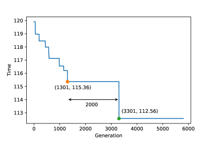
Figure 7: The objective function of instance B6 over generations, solved by HGA-TAC⁺.

6 Conclusions

This paper presents a Hybrid Genetic Algorithm with Type-Aware Chromosome encoding (HGA-TAC), to solve TSPD and FSTSP. The GA is responsible for partitioning and managing the sequences of the customers, while the DP is responsible for determining the rendezvous points and calculating the objective value. TSPD and FSTSP both aim to find the best routes for trucks and drones, yet several assumptions differ slightly between the two. There were several local search methods offered, along with two crossover approaches that were specifically designed for our problem. Additionally, we developed an escaping strategy, which circumvents the local optima and can be applied to any Genetic Algorithm in general.

As evidenced by our testing on five benchmark sets of instances, our GA either exceeds or is competitive with the best existing methods. We believe the faster performance in our method is due to making the decisions about the sequence and node types by GA and leaving less information to be decided optimally by DP. Moreover, it was observed that Escape Local improved the quality of the solution at the cost of increased running time.

A few future research directions may be considered. A generalized version of the proposed method can be implemented using multiple drones in conjunction with a truck in order to solve the TSPD. A further extension could involve allowing the drone to visit more than one customer in a single operation. Furthermore, the proposed method in this paper could be extended to vehicle routing problems with drones, where a fleet of multiple trucks and multiple drones is routed.

Appendix: Tables representing the details of experiments

Table 4: (TSPD Set-A, $\alpha=1$) Results of HGA-TAC and HGA-TAC⁺ for Agatz et al. (2018) instances with $\alpha=1$. Times are in seconds, and Time* is as reported in de Freitas and Penna (2020).

HGVNS DPS/25 HGA-TAC Gap Over (%) HGA-TAC⁺ Gap Over (%) Dist $N$ Obj Time* Obj Time Obj Time HGVNS DPS/25 Obj Time HGVNS DPS/25 Uniform 10 289.82 0.14 265.20 0.01 265.20 0.23 $-$8.49 0.00 265.20 0.70 $-$8.49 0.00 20 368.54 0.11 325.23 0.06 326.40 0.49 $-$11.43 0.36 324.76 1.78 $-$11.88 $-$0.15 50 559.20 3.71 498.20 0.26 498.45 1.55 $-$10.86 0.05 493.84 6.54 $-$11.69 $-$0.87 75 624.32 16.30 574.21 0.39 576.40 2.66 $-$7.68 0.38 572.61 11.50 $-$8.28 $-$0.28 100 698.42 53.50 655.87 0.54 659.41 3.89 $-$5.59 0.54 652.00 19.29 $-$6.65 $-$0.59 175 905.32 55.91 841.39 1.56 843.36 9.27 $-$6.84 0.23 837.72 48.17 $-$7.47 $-$0.44 250 1135.32 185.19 988.59 2.26 982.64 21.33 $-$13.45 $-$0.60 978.43 112.67 $-$13.82 $-$1.03 Average 44.98 0.73 5.63 $-$9.19 0.14 28.66 $-$9.75 $-$0.48 Single Center 10 364.92 0.13 335.29 0.01 335.27 0.21 $-$8.12 0.00 335.27 0.70 $-$8.12 0.00 20 553.53 0.85 462.1 0.06 458.74 0.51 $-$17.13 $-$0.73 458.30 1.84 $-$17.20 $-$0.82 50 784.32 2.30 657.79 0.27 654.67 2.06 $-$16.53 $-$0.47 650.62 8.68 $-$17.05 $-$1.09 75 978.32 10.93 890.12 0.48 884.49 3.02 $-$9.59 $-$0.63 878.59 14.74 $-$10.19 $-$1.30 100 1193.95 37.77 1065.77 0.57 1061.36 5.25 $-$11.10 $-$0.41 1053.90 23.25 $-$11.73 $-$1.11 175 1629.32 39.28 1420.95 1.31 1421.04 11.45 $-$12.78 0.01 1412.82 68.86 $-$13.29 $-$0.57 250 1813.54 191.48 1646.00 1.94 1645.99 18.61 $-$9.24 0.00 1636.44 146.19 $-$9.77 $-$0.58 Average 40.39 0.66 5.87 $-$12.07 $-$0.32 37.75 $-$12.48 $-$0.78 Double Center 10 634.42 0.14 586.6 0.01 586.60 0.20 $-$7.54 0.00 586.60 0.66 $-$7.54 0.00 20 754.81 0.11 709.79 0.08 711.46 0.50 $-$5.74 0.23 711.58 1.73 $-$5.73 0.25 50 1203.09 3.71 1010.88 0.28 1002.62 2.08 $-$16.66 $-$0.82 993.95 8.05 $-$17.38 $-$1.67 75 1494.57 16.30 1243.47 0.43 1239.43 3.66 $-$17.07 $-$0.32 1229.48 15.58 $-$17.74 $-$1.13 100 1556.52 53.50 1405.57 0.59 1393.82 5.23 $-$10.45 $-$0.84 1383.34 24.02 $-$11.13 $-$1.58 175 2072.36 55.91 1910.03 1.22 1912.26 12.92 $-$7.73 0.12 1898.27 65.24 $-$8.40 $-$0.62 250 2523.00 185.19 2275.4 1.77 2273.47 20.96 $-$9.89 $-$0.08 2263.12 135.06 $-$10.30 $-$0.54 Average 44.98 0.63 6.51 $-$10.73 $-$0.24 35.76 $-$11.17 $-$0.76

Table 5: (TSPD Set-A, $\alpha=2$) Results of HGA-TAC and HGA-TAC⁺ for Agatz et al. (2018) instances with $\alpha=2$. Times are in seconds, and Time* is as reported in de Freitas and Penna (2020).

HGVNS DPS/25 HGA-TAC Gap Over (%) HGA-TAC⁺ Gap Over (%) Dist $N$ Obj Time* Obj Time Obj Time HGVNS DPS/25 Obj Time HGVNS DPS/25 Uniform 10 233.20 0.13 218.57 0.01 218.04 0.17 $-$6.50 $-$0.24 218.08 0.54 $-$6.49 $-$0.22 20 293.60 0.85 277.51 0.11 274.87 0.36 $-$6.38 $-$0.95 274.19 1.25 $-$6.61 $-$1.20 50 420.80 2.30 420.60 0.59 415.69 1.38 $-$1.21 $-$1.17 408.00 4.96 $-$3.04 $-$2.99 75 490.43 10.93 482.16 0.81 484.13 2.77 $-$1.28 0.41 473.58 9.99 $-$3.44 $-$1.78 100 553.43 37.77 559.52 1.06 564.05 4.54 1.92 0.81 551.17 17.36 $-$0.41 $-$1.49 175 704.53 39.28 711.85 2.91 724.53 13.10 2.84 1.78 703.67 70.72 $-$0.12 $-$1.15 250 824.42 191.48 837.04 3.21 850.17 26.93 3.12 1.57 827.24 202.02 0.34 $-$1.17 Average 40.39 1.24 7.03 $-$1.07 0.32 43.83 $-$2.82 $-$1.43 Single Center 10 291.36 0.14 261.61 0.01 260.33 0.18 $-$10.65 $-$0.49 260.40 0.61 $-$10.63 $-$0.46 20 364.08 1.04 351.06 0.09 352.55 0.42 $-$3.17 0.42 349.54 1.57 $-$3.99 $-$0.43 50 593.54 2.23 521.66 0.55 515.72 1.57 $-$13.11 $-$1.14 510.63 4.86 $-$13.97 $-$2.12 75 754.43 11.18 715.27 0.90 712.99 3.28 $-$5.49 $-$0.32 703.45 10.43 $-$6.76 $-$1.65 100 900.12 38.23 858.12 1.10 873.27 5.39 $-$2.98 1.77 856.52 19.53 $-$4.84 $-$0.19 175 1183.43 43.06 1157.29 2.09 1178.93 16.22 $-$0.38 1.87 1156.92 78.61 $-$2.24 $-$0.03 250 1294.43 197.12 1339.34 3.46 1375.14 36.45 6.24 2.67 1347.80 214.73 4.12 0.63 Average 41.86 1.17 9.07 $-$4.22 0.68 47.19 $-$5.47 $-$0.61 Double Center 10 510.09 0.13 467.14 0.01 465.00 0.16 $-$8.84 $-$0.46 464.97 0.55 $-$8.85 $-$0.46 20 605.04 0.98 590.99 0.12 587.47 0.40 $-$2.90 $-$0.60 586.89 1.31 $-$3.00 $-$0.69 50 850.31 2.24 825.09 0.49 813.72 1.71 $-$4.30 $-$1.38 800.86 5.52 $-$5.82 $-$2.94 75 1123.61 11.61 1018.52 0.85 1012.58 3.57 $-$9.88 $-$0.58 994.88 11.76 $-$11.46 $-$2.32 100 1199.09 38.22 1138.35 1.11 1153.25 6.05 $-$3.82 1.31 1139.70 20.22 $-$4.95 0.12 175 1659.37 42.31 1568.74 2.11 1601.50 16.21 $-$3.49 2.09 1567.70 76.79 $-$5.52 $-$0.07 250 1862.44 193.17 1862.93 3.03 1931.15 33.94 3.69 3.66 1894.26 212.31 1.71 1.68 Average 41.24 1.10 8.86 $-$4.22 0.58 46.92 $-$5.41 $-$0.67

Table 6: (TSPD Set-A, $\alpha=3$) Results of HGA-TAC and HGA-TAC⁺ for Agatz et al. (2018) instances with $\alpha=3$. Times are in seconds, and Time* is as reported in de Freitas and Penna (2020).

HGVNS DPS/25 HGA-TAC Gap Over (%) HGA-TAC⁺ Gap Over (%) Dist $N$ Obj Time* Obj Time Obj Time HGVNS DPS/25 Obj Time HGVNS DPS/25 uniform 10 215.88 0.13 203.32 0.01 198.70 0.15 $-$7.96 $-$2.28 198.97 0.51 $-$7.83 $-$2.14 20 274.20 1.15 256.18 0.14 252.45 0.35 $-$7.93 $-$1.46 252.63 1.11 $-$7.87 $-$1.39 50 389.80 2.19 393.12 0.73 385.36 1.37 $-$1.14 $-$1.98 375.70 4.48 $-$3.62 $-$4.43 75 447.64 10.95 454.50 0.97 448.65 2.95 0.23 $-$1.29 433.19 10.58 $-$3.23 $-$4.69 100 510.20 37.26 530.17 1.43 524.85 5.45 2.87 $-$1.00 509.00 18.25 $-$0.23 $-$3.99 175 655.20 41.49 670.67 3.78 674.81 15.78 2.99 0.62 646.13 91.43 $-$1.38 $-$3.66 250 758.32 189.43 792.99 4.18 801.46 33.30 5.69 1.07 765.79 268.35 0.98 $-$3.43 Average 40.37 1.61 8.48 $-$0.75 $-$0.90 56.39 $-$3.31 $-$3.39 Single center 10 242.20 0.13 224.38 0.01 219.86 0.15 $-$9.22 $-$2.01 219.71 0.53 $-$9.29 $-$2.08 20 319.80 0.86 295.93 0.15 293.13 0.39 $-$8.34 $-$0.95 291.33 1.33 $-$8.90 $-$1.55 50 493.43 2.19 471.78 0.71 452.29 1.67 $-$8.34 $-$4.13 442.38 5.09 $-$10.35 $-$6.23 75 638.20 11.39 647.68 1.23 635.32 3.92 $-$0.45 $-$1.91 619.76 10.70 $-$2.89 $-$4.31 100 804.43 37.74 777.00 1.47 772.90 6.50 $-$3.92 $-$0.53 759.03 21.32 $-$5.64 $-$2.31 175 998.53 41.20 1048.29 2.71 1063.19 21.44 6.48 1.42 1030.37 95.83 3.19 $-$1.71 250 1224.43 198.72 1233.68 3.94 1241.86 44.01 1.42 0.66 1206.40 300.99 $-$1.47 $-$2.21 Average 41.75 1.46 11.15 $-$3.20 $-$1.06 62.26 $-$5.05 $-$2.92 Double Center 10 439.60 0.13 421.94 0.01 413.14 0.15 $-$6.02 $-$2.08 413.14 0.51 $-$6.02 $-$2.08 20 586.74 0.99 560.54 0.14 548.91 0.37 $-$6.45 $-$2.07 548.11 1.06 $-$6.58 $-$2.22 50 746.93 2.14 760.15 0.71 739.64 1.60 $-$0.98 $-$2.70 726.96 4.64 $-$2.67 $-$4.37 75 945.34 11.22 934.53 1.01 912.43 3.89 $-$3.48 $-$2.36 896.01 11.00 $-$5.22 $-$4.12 100 1102.64 37.86 1034.77 1.60 1038.42 7.16 $-$5.82 0.35 1014.65 20.51 $-$7.98 $-$1.94 175 1469.92 41.58 1453.16 2.74 1457.59 21.84 $-$0.84 0.30 1408.44 107.60 $-$4.18 $-$3.08 250 1635.12 196.27 1709.35 3.78 1762.70 44.51 7.80 3.12 1701.57 314.41 4.06 $-$0.46 Average 41.46 1.43 11.36 $-$2.25 $-$0.78 65.67 $-$4.08 $-$2.61

Table 7: (TSPD Set-A, limited) Results of HGA-TAC and HGA-TAC⁺ for Agatz et al. (2018)’s instances with limited flying ranges, where $r$ is a parameter in the dataset that controls the maximum flying range. Times are in seconds.

TSP-ep-all DPS/25 HGA-TAC Gap over (%) HGA-TAC⁺ Gap over (%) $N$ $r$ Obj Time Obj Time Mean Time TSP-ep-all DPS/25 Mean Time TSP-ep-all DPS/25 10 20 303.74 0.01 303.74 0.01 303.74 0.27 0.00 0.00 303.74 0.79 0.00 0.00 40 295.73 0.01 295.73 0.01 295.60 0.28 $-$0.04 $-$0.04 295.58 0.77 $-$0.05 $-$0.05 60 277.12 0.01 277.12 0.01 276.09 0.24 $-$0.37 $-$0.37 275.90 0.73 $-$0.44 $-$0.44 100 236.02 0.01 236.02 0.01 235.47 0.23 $-$0.23 $-$0.23 235.30 0.69 $-$0.31 $-$0.31 150 219.41 0.01 219.41 0.01 219.35 0.23 $-$0.03 $-$0.03 219.13 0.68 $-$0.13 $-$0.13 200 218.57 0.01 218.57 0.01 218.19 0.21 $-$0.17 $-$0.17 218.07 0.54 $-$0.23 $-$0.23 Average 0.01 0.01 0.24 $-$0.14 $-$0.14 0.70 $-$0.19 $-$0.19 20 5 396.30 0.03 396.30 0.03 396.30 0.50 0.00 0.00 396.30 1.69 0.00 0.00 10 396.08 0.03 396.08 0.03 396.08 0.54 0.00 0.00 396.08 1.71 0.00 0.00 15 394.58 0.03 394.58 0.03 394.50 0.58 $-$0.02 $-$0.02 394.47 1.75 $-$0.03 $-$0.03 20 387.57 0.04 387.57 0.04 387.02 0.59 $-$0.14 $-$0.14 386.76 1.72 $-$0.21 $-$0.21 30 359.79 0.04 359.79 0.04 359.98 0.53 0.05 0.05 359.45 1.63 $-$0.10 $-$0.10 40 344.60 0.05 344.60 0.05 343.70 0.45 $-$0.26 $-$0.26 342.69 1.35 $-$0.56 $-$0.56 50 322.02 0.05 322.02 0.05 320.00 0.47 $-$0.63 $-$0.63 319.45 1.41 $-$0.80 $-$0.80 Average 0.04 0.04 0.53 $-$0.17 $-$0.17 1.59 $-$0.28 $-$0.28 50 5 595.57 0.53 595.57 0.08 595.58 2.38 0.00 0.00 595.57 8.07 0.00 0.00 10 587.29 0.95 587.49 0.11 587.36 2.01 0.01 $-$0.02 587.25 5.93 $-$0.01 $-$0.04 15 561.82 1.32 564.59 0.13 562.97 1.72 0.20 $-$0.29 561.40 5.92 $-$0.08 $-$0.57 20 514.65 1.63 516.89 0.15 519.11 1.54 0.87 0.43 516.54 5.34 0.37 $-$0.07 30 451.17 2.55 459.20 0.20 456.73 1.55 1.23 $-$0.54 451.88 5.21 0.16 $-$1.59 40 418.46 3.85 431.86 0.25 426.10 1.98 1.83 $-$1.33 420.90 6.32 0.58 $-$2.54 50 414.27 6.22 427.90 0.32 421.46 2.03 1.74 $-$1.51 413.24 7.22 $-$0.25 $-$3.43 Average 2.75 0.19 1.80 0.98 $-$0.54 5.99 0.13 $-$1.37 75 5 629.48 3.29 629.48 0.13 629.56 4.85 0.01 0.01 629.45 15.06 0.00 0.00 10 603.19 6.96 604.30 0.17 604.32 2.47 0.19 0.00 603.39 8.36 0.03 $-$0.15 15 553.38 12.81 557.19 0.24 559.43 2.44 1.09 0.40 556.27 9.02 0.52 $-$0.17 20 508.73 18.20 515.90 0.30 520.68 2.44 2.35 0.93 513.74 10.07 0.99 $-$0.42 30 449.88 26.65 459.52 0.37 459.09 3.19 2.05 $-$0.10 452.11 10.65 0.49 $-$1.61 40 436.16 49.10 445.09 0.49 449.37 3.25 3.03 0.96 440.41 12.68 0.98 $-$1.05 50 433.02 80.76 439.36 0.62 445.77 3.10 2.95 1.46 435.56 12.91 0.59 $-$0.87 Average 28.25 0.33 3.11 1.67 0.52 11.25 0.51 $-$0.61 100 5 780.32 13.58 780.43 0.18 780.38 9.14 0.01 $-$0.01 780.34 30.27 0.00 $-$0.01 10 728.87 34.05 731.13 0.23 730.57 3.51 0.23 $-$0.08 729.00 13.55 0.02 $-$0.29 15 654.82 64.33 660.33 0.33 664.36 3.48 1.46 0.61 660.37 14.32 0.85 0.01 30 555.81 130.23 567.71 0.57 572.83 4.86 3.06 0.90 563.69 17.98 1.42 $-$0.71 50 547.41 497.45 559.12 0.90 572.26 4.37 4.54 2.35 557.19 21.93 1.79 $-$0.34 Average 147.93 0.44 5.07 1.86 0.76 19.61 0.81 $-$0.27

Table 8: (TSPD Set-B) TSPD results on the datasets of Bogyrbayeva et al. (2023). Average cost and time values are reported on 100 problem instances for each size $N$. Times are in seconds, and Time* is as reported in Bogyrbayeva et al. (2023). Gap values are measured, in $\%$, over the Obj values of TSP-ep-all, and the Mean values are used for HGA-TAC and HGA-TAC⁺.

TSP-ep-all DPS/25 HM (4800) HGA-TAC HGA-TAC⁺ Dataset $N$ Obj Time Obj Time Gap Obj Time* Gap Best Mean Time Gap Best Mean Time Gap Random 20 281.85 0.10 281.85 0.01 0.00 281.53 0.40 $-$0.11 278.25 280.42 0.36 $-$0.51 277.82 279.54 1.19 $-$0.82 50 397.63 21.99 404.88 0.54 1.82 395.65 1.72 $-$0.50 394.64 402.52 1.36 1.23 389.12 396.11 4.69 $-$0.38 100 535.20 2566.28 548.08 1.14 2.41 544.55 4.09 1.75 541.71 551.38 4.68 3.02 530.57 538.95 18.59 0.70 Average 404.89 862.79 411.60 0.56 1.41 407.24 2.07 0.38 404.87 411.44 2.13 1.25 399.17 404.87 8.16 $-$0.17 Amesterdam 10 2.02 0.02 2.02 0.02 0.00 2.04 0.32 0.99 2.00 2.01 0.17 $-$0.50 2.00 2.00 0.57 $-$0.99 20 2.36 0.09 2.36 0.09 0.00 2.38 0.52 0.85 2.32 2.34 0.36 $-$0.84 2.32 2.33 1.35 $-$1.27 50 3.26 21.92 3.37 0.56 2.58 3.31 1.41 1.53 3.27 3.35 1.55 2.76 3.23 3.31 4.94 1.53 Average 2.55 7.34 2.58 0.22 1.12 2.58 0.75 1.12 2.53 2.57 0.69 0.47 2.52 2.55 2.29 $-$0.24

Table 9: (FSTSP Set-M) Results for FSTSP instances from Murray and Chu (2015). MC and HGA20 represent the results reported by Murray and Chu (2015) and Ha et al. (2020), respectively. Times are in seconds. Gap values are measured, in $\%$, between the Mean values of HGA-TAC and HGA-TAC⁺ and the Mean values of HGA20.

			HGA20			HGA-TAC					HGA-TAC+
Instance	$\epsilon$	MC	Best	Mean		Best	Mean	Time	Gap		Best	Mean	Time	Gap
437v1	20	56.468	56.468	56.468		56.393	56.393	0.44	$-$0.13		56.393	56.393	1.44	$-$0.13
437v1	40	50.573	50.573	50.573		50.573	50.573	0.26	0.00		50.573	50.573	1.15	0.00
437v2	20	53.207	53.207	53.207		50.947	50.947	0.23	$-$4.25		50.947	50.947	1.10	$-$4.25
437v2	40	47.311	47.311	47.311		47.311	48.580	0.21	2.68		47.311	49.082	0.90	3.74
437v3	20	53.687	53.687	53.687		54.664	54.664	0.27	1.82		54.664	54.664	1.16	1.82
437v3	40	53.687	53.687	53.687		51.427	51.427	0.21	$-$4.21		51.427	51.427	0.93	$-$4.21
437v4	20	67.464	67.464	67.464		67.464	67.464	0.27	0.00		67.464	67.464	1.10	0.00
437v4	40	66.487	66.487	66.487		64.227	64.227	0.28	$-$3.40		64.227	64.227	0.96	$-$3.40
437v5	20	50.551	50.551	50.551		47.677	48.017	0.27	$-$5.01		47.677	47.928	1.11	$-$5.19
437v5	40	45.835	44.835	44.835		44.835	45.524	0.28	1.54		44.835	45.035	1.01	0.45
437v6	20	45.176	47.311	47.311		45.287	45.287	0.24	$-$4.28		45.287	45.287	1.11	$-$4.28
437v6	40	45.863	43.602	43.602		43.602	43.743	0.27	0.32		43.602	43.622	1.00	0.05
437v7	20	49.581	49.581	49.581		46.131	46.144	0.24	$-$6.93		46.131	46.131	1.12	$-$6.96
437v7	40	46.621	46.621	46.621		45.555	45.555	0.27	$-$2.29		45.555	45.555	1.03	$-$2.29
437v8	20	62.381	62.381	62.381		58.784	58.784	0.30	$-$5.77		58.784	58.784	1.69	$-$5.77
437v8	40	59.776	59.416	59.416		58.355	58.363	0.23	$-$1.77		58.355	58.363	1.33	$-$1.77
437v9	20	45.985	42.416	42.416		40.284	41.468	0.26	$-$2.23		40.284	41.200	1.16	$-$2.87
437v9	40	42.416	42.416	42.416		39.922	40.910	0.29	$-$3.55		39.922	40.722	1.09	$-$3.99
437v10	20	42.416	41.729	41.729		40.541	40.897	0.30	$-$1.99		39.728	40.216	1.26	$-$3.63
437v10	40	41.729	41.729	41.729		40.179	40.225	0.22	$-$3.60		40.179	40.225	1.06	$-$3.60
437v11	20	42.896	42.896	42.896		41.896	41.925	0.31	$-$2.26		41.896	41.955	1.21	$-$2.19
437v11	40	42.896	42.896	42.896		42.896	42.896	0.26	0.00		42.896	42.896	1.11	0.00
437v12	20	56.696	56.273	56.273		54.992	54.992	0.24	$-$2.28		54.992	54.992	1.20	$-$2.28
437v12	40	55.696	55.696	55.696		54.285	54.351	0.22	$-$2.41		54.285	54.285	0.89	$-$2.53
440v1	20	49.430	49.430	49.430		48.430	48.430	0.27	$-$2.02		48.430	48.430	1.12	$-$2.02
440v1	40	46.886	46.886	46.886		46.514	46.588	0.30	$-$0.63		46.514	46.551	1.44	$-$0.71
440v2	20	50.708	50.708	50.708		50.708	50.708	0.23	0.00		50.708	50.708	1.12	0.00
440v2	40	46.423	46.423	46.423		46.423	46.423	0.26	0.00		46.423	46.423	1.46	0.00
440v3	20	56.102	56.102	56.102		56.102	56.102	0.19	0.00		56.102	56.102	1.19	0.00
440v3	40	53.933	53.933	53.933		53.933	53.933	0.23	0.00		53.933	53.933	1.51	0.00
440v4	20	69.902	69.902	69.902		68.902	68.902	0.22	$-$1.43		68.902	68.902	1.89	$-$1.43
440v4	40	68.397	68.397	68.397		67.397	67.397	0.24	$-$1.46		67.397	67.397	1.34	$-$1.46
440v5	20	43.533	43.533	43.533		44.456	44.456	0.31	2.12		44.456	44.456	1.21	2.12
440v5	40	43.533	43.533	43.533		43.533	43.533	0.27	0.00		43.533	43.533	1.17	0.00
440v6	20	44.076	43.949	43.949		43.949	43.949	0.29	0.00		43.949	43.949	1.17	0.00
440v6	40	44.076	43.810	43.853		43.253	43.253	0.31	$-$1.37		43.253	43.253	1.20	$-$1.37
440v7	20	49.996	49.422	49.422		48.422	48.422	0.28	$-$2.02		48.422	48.422	1.18	$-$2.02
440v7	40	49.204	49.204	49.204		48.470	48.470	0.33	$-$1.49		48.470	48.470	1.25	$-$1.49
440v8	20	62.796	62.576	62.576		61.222	61.222	0.25	$-$2.16		61.222	61.222	1.12	$-$2.16
440v8	40	62.270	62.004	62.004		61.270	61.270	0.24	$-$1.18		61.270	61.270	1.07	$-$1.18
440v9	20	42.799	42.533	42.533		41.799	42.092	0.24	$-$1.04		40.342	41.521	1.07	$-$2.38
440v9	40	42.799	42.533	42.533		42.005	42.459	0.28	$-$0.17		40.342	41.335	1.34	$-$2.82
440v10	20	43.076	43.076	43.076		40.412	41.083	0.25	$-$4.63		40.412	40.748	1.07	$-$5.41
440v10	40	43.076	43.076	43.076		40.412	40.744	0.24	$-$5.41		40.412	40.664	1.07	$-$5.60
440v11	20	49.204	49.204	49.204		44.944	46.844	0.24	$-$4.80		44.944	46.405	1.07	$-$5.69
440v11	40	49.204	49.204	49.204		45.364	46.727	0.27	$-$5.04		44.944	46.162	1.09	$-$6.18
440v12	20	62.004	62.004	62.004		56.957	58.953	0.20	$-$4.92		56.957	58.542	1.29	$-$5.58
440v12	40	62.004	62.004	62.004		56.882	57.502	0.22	$-$7.26		56.882	57.138	1.81	$-$7.85
443v1	20	69.586	69.586	69.586		69.586	69.586	0.27	0.00		69.586	69.586	1.13	0.00
443v1	40	55.493	55.493	55.493		56.676	56.676	0.31	2.13		56.676	56.843	1.17	2.43
443v2	20	72.146	72.146	72.146		72.146	72.146	0.23	0.00		72.146	72.146	1.01	0.00
443v2	40	58.053	58.053	58.053		58.053	58.053	0.22	0.00		58.053	58.053	0.97	0.00
443v3	20	77.344	77.344	77.344		76.374	76.567	0.21	$-$1.00		76.374	76.466	0.97	$-$1.14
443v3	40	69.175	68.431	68.431		68.918	68.918	0.21	0.71		68.918	68.918	0.97	0.71
443v4	20	90.144	90.144	90.144		89.404	89.404	0.27	$-$0.82		89.404	89.404	1.04	$-$0.82
443v4	40	82.700	82.700	82.700		81.818	81.818	0.21	$-$1.07		81.818	81.818	0.97	$-$1.07
443v5	20	55.493	54.973	55.077		56.477	56.848	0.26	3.22		56.477	56.877	1.13	3.27
443v5	40	53.447	51.929	51.929		45.676	45.676	0.30	$-$12.04		45.676	45.676	1.17	$-$12.04
443v6	20	58.053	55.209	55.209		57.006	57.114	0.27	3.45		57.006	57.438	1.20	4.04
443v6	40	52.329	52.329	52.329		48.236	48.236	0.31	$-$7.82		48.236	48.236	1.24	$-$7.82
443v7	20	64.409	65.523	65.523		62.046	62.046	0.27	$-$5.31		62.046	62.046	1.16	$-$5.31
443v7	40	60.743	60.743	60.743		57.119	57.119	0.35	$-$5.97		57.119	57.119	1.21	$-$5.97
443v8	20	77.209	78.323	78.323		78.343	79.267	0.31	1.21		78.343	79.461	1.12	1.45
443v8	40	73.967	72.967	72.967		69.317	69.317	0.25	$-$5.00		69.317	69.317	1.05	$-$5.00
443v9	20	49.049	45.931	45.931		42.691	42.691	0.30	$-$7.05		42.691	42.691	1.10	$-$7.05
443v9	40	47.250	45.931	45.931		42.691	42.691	0.26	$-$7.05		42.691	42.691	1.06	$-$7.05
443v10	20	47.935	46.935	46.935		43.061	43.061	0.27	$-$8.25		43.061	43.061	1.04	$-$8.25
443v10	40	47.935	46.935	46.935		43.061	43.061	0.33	$-$8.25		43.061	43.061	1.01	$-$8.25
443v11	20	57.382	56.395	56.395		52.964	53.466	0.39	$-$5.19		52.964	53.403	1.39	$-$5.31
443v11	40	56.395	56.395	56.395		52.964	53.464	0.33	$-$5.20		52.964	53.464	1.08	$-$5.20
443v12	20	69.195	69.195	69.195		67.391	67.391	0.24	$-$2.61		67.391	67.391	1.02	$-$2.61
443v12	40	69.195	69.195	69.195		64.894	64.894	0.21	$-$6.22		64.528	64.711	0.98	$-$6.48
	Average	55.215	54.937	54.939		53.429	53.643	0.27	$-$2.40		53.364	53.575	1.16	$-$2.56

Table 10: (FSTSP Set-H) Results for FSTSP instances from Ha et al. (2018). Times are in seconds, and Time* represents the time reported in Ha et al. (2018). Gap is measured between the Mean values of HGA-TAC and HGA-TAC⁺ and the Mean values of HGA20.

	HGA20				HGA-TAC					HGA-TAC+
Instance	Best	Mean	Time*		Best	Mean	Gap	Time		Best	Mean	Gap	Time
B1	115.65	116.43	45.60		116.92	117.23	0.69	2.73		115.11	115.89	$-$0.46	12.26
B2	118.39	118.39	19.80		113.93	114.17	$-$3.56	1.69		113.50	113.82	$-$3.86	9.06
B3	116.21	116.39	34.20		114.09	114.75	$-$1.41	2.59		112.25	113.52	$-$2.46	10.57
B4	118.71	119.26	28.20		119.85	121.77	2.11	2.05		119.19	120.88	1.35	10.38
B5	115.78	115.91	34.80		113.77	114.38	$-$1.32	1.84		112.77	114.44	$-$1.27	6.02
B6	114.31	115.46	52.80		114.04	115.25	$-$0.18	2.87		112.11	112.69	$-$2.40	12.07
B7	115.52	115.63	37.20		115.53	117.84	1.91	2.67		113.63	115.02	$-$0.52	12.56
B8	117.90	118.04	46.80		113.25	114.13	$-$3.32	2.41		113.25	113.70	$-$3.68	10.00
B9	117.64	117.72	23.40		116.23	117.14	$-$0.49	1.87		116.23	116.90	$-$0.69	7.89
B10	117.38	117.70	36.00		114.28	115.31	$-$2.03	2.77		114.28	115.04	$-$2.26	8.55
C1	215.07	215.37	36.00		214.91	216.34	0.45	2.12		211.80	212.38	$-$1.39	11.43
C2	209.23	210.11	31.80		202.41	202.82	$-$3.47	1.28		202.41	202.90	$-$3.43	4.03
C3	212.02	212.22	22.80		204.79	204.97	$-$3.42	1.29		204.79	204.97	$-$3.42	3.92
C4	212.08	213.27	36.00		215.25	218.72	2.55	1.75		212.17	215.12	0.87	9.43
C5	223.06	224.57	28.80		225.54	225.54	0.43	1.36		225.54	225.54	0.43	4.14
C6	234.01	235.56	18.60		233.57	233.57	$-$0.84	1.29		233.57	233.57	$-$0.84	4.10
C7	222.27	223.40	30.60		218.98	220.10	$-$1.48	2.27		219.00	219.49	$-$1.75	8.14
C8	234.26	237.53	27.60		233.44	234.68	$-$1.20	2.17		233.24	234.18	$-$1.41	8.22
C9	226.01	227.43	40.80		222.60	224.43	$-$1.32	1.15		222.60	224.73	$-$1.19	3.59
C10	226.17	226.17	28.80		222.99	223.88	$-$1.01	1.48		222.63	223.62	$-$1.13	6.50
D1	306.39	307.09	36.60		312.78	314.32	2.35	2.14		312.78	313.40	2.05	8.10
D2	313.93	315.64	34.20		306.78	308.79	$-$2.17	1.80		305.80	307.70	$-$2.52	5.84
D3	295.86	297.54	36.00		289.49	290.96	$-$2.21	3.17		286.82	288.30	$-$3.11	10.01
D4	323.72	324.60	33.60		320.80	321.96	$-$0.81	2.42		319.25	320.94	$-$1.13	7.88
D5	321.46	321.83	24.00		315.75	316.46	$-$1.67	2.27		313.82	314.08	$-$2.41	8.47
D6	313.21	313.65	29.40		307.81	308.06	$-$1.78	1.98		307.81	307.87	$-$1.84	6.34
D7	316.65	317.83	19.20		312.23	315.81	$-$0.64	2.40		309.42	314.25	$-$1.13	7.99
D8	293.76	296.51	34.80		291.31	294.37	$-$0.72	2.53		288.53	294.13	$-$0.80	6.14
D9	317.85	318.31	24.60		326.99	327.62	2.92	1.11		326.99	327.46	2.87	3.29
D10	305.51	305.54	24.60		298.20	300.20	$-$1.75	2.23		297.58	298.89	$-$2.18	7.03
E1	187.67	188.32	216.00		178.77	181.24	$-$3.76	8.63		177.03	178.10	$-$5.42	37.01
E2	187.21	188.01	336.00		182.60	183.51	$-$2.39	6.88		180.11	181.35	$-$3.54	27.21
E3	188.09	188.89	274.80		179.24	180.28	$-$4.56	7.40		177.22	178.42	$-$5.54	36.17
E4	186.23	186.99	281.40		182.80	185.38	$-$0.86	7.69		177.92	179.75	$-$3.87	51.61
E5	187.71	188.26	243.60		181.85	183.62	$-$2.47	7.07		179.50	182.04	$-$3.30	32.81
E6	189.16	189.44	290.40		182.25	183.46	$-$3.16	10.83		179.65	181.05	$-$4.43	45.30
E7	190.39	190.89	230.40		184.40	185.52	$-$2.81	10.75		181.05	182.41	$-$4.44	54.15
E8	189.02	189.54	253.20		182.10	182.84	$-$3.53	9.33		179.97	180.72	$-$4.65	41.37
E9	189.76	189.94	240.00		181.53	183.61	$-$3.33	8.69		179.20	180.70	$-$4.87	51.66
E10	189.45	189.91	204.00		184.79	184.84	$-$2.67	5.04		184.84	184.84	$-$2.67	17.90
F1	322.94	326.10	343.80		326.89	334.71	2.64	5.64		322.88	329.92	1.17	26.79
F2	308.74	310.89	314.40		310.48	316.07	1.66	4.16		305.40	309.56	$-$0.43	28.95
F3	309.67	313.55	336.60		322.41	323.23	3.09	2.37		322.41	322.90	2.98	7.81
F4	311.37	314.96	363.60		320.15	320.25	1.68	2.47		320.15	320.25	1.68	7.83
F5	314.82	317.83	394.20		322.93	324.89	2.22	2.52		321.33	324.76	2.18	9.31
F6	294.38	297.47	282.00		293.17	296.78	$-$0.23	7.92		288.86	292.16	$-$1.79	39.54
F7	311.41	316.15	295.20		307.14	308.15	$-$2.53	5.18		304.08	306.05	$-$3.19	22.09
F8	323.74	326.40	312.60		325.76	327.16	0.23	2.23		325.76	329.98	1.10	7.21
F9	315.56	318.47	279.60		327.85	328.11	3.03	2.22		327.85	327.98	2.99	7.19
F10	312.70	315.13	236.40		318.68	319.14	1.27	2.34		318.68	319.14	1.27	7.53
G1	417.92	425.19	267.00		412.54	414.79	$-$2.45	6.75		409.57	411.53	$-$3.21	31.62
G2	389.64	390.14	144.00		397.37	401.86	3.00	5.35		388.18	401.98	3.03	16.31
G3	411.47	415.14	294.00		423.77	426.58	2.75	6.20		421.24	422.68	1.82	28.78
G4	433.09	435.56	280.20		430.63	431.62	$-$0.90	2.32		430.63	431.43	$-$0.95	7.33
G5	421.05	422.49	268.80		421.60	422.01	$-$0.11	2.21		416.34	419.82	$-$0.63	15.96
G6	415.46	420.84	330.60		426.26	433.17	2.93	3.53		425.39	430.77	2.36	14.80
G7	409.31	412.14	312.60		403.57	403.61	$-$2.07	2.13		403.57	403.66	$-$2.06	6.85
G8	406.51	407.89	304.80		423.31	427.04	4.70	6.74		413.32	421.51	3.34	28.44
G9	428.16	435.75	354.60		440.10	444.52	2.01	4.97		438.46	441.23	1.26	26.69
G10	426.82	430.94	324.00		435.84	438.78	1.82	2.32		435.84	438.78	1.82	7.32
Average	260.99	262.64	159.44		260.66	262.37	$-$0.47	3.73		258.92	260.85	$-$1.13	16.29

References

- Agatz et al. (2018) Agatz, N., P. Bouman, M. Schmidt. 2018. Optimization approaches for the traveling salesman problem with drone. Transportation Science 52(4) 965–981.
- Boccia et al. (2021) Boccia, M., A. Masone, A. Sforza, C. Sterle. 2021. A column-and-row generation approach for the flying sidekick travelling salesman problem. Transportation Research Part C: Emerging Technologies 124 102913.
- Bogyrbayeva et al. (2023) Bogyrbayeva, A., T. Yoon, H. Ko, S. Lim, H. Yun, C. Kwon. 2023. A deep reinforcement learning approach for solving the traveling salesman problem with drone. Transportation Research Part C: Emerging Technologies 103981.
- Bouman et al. (2018) Bouman, P., N. Agatz, M. Schmidt. 2018. Dynamic programming approaches for the traveling salesman problem with drone. Networks 72(4) 528–542.
- Campuzano et al. (2021) Campuzano, G., E. Lalla-Ruiz, M. Mes. 2021. A multi-start vns algorithm for the tsp-d with energy constraints. International Conference on Computational Logistics. Springer, 393–409.
- Chung et al. (2020) Chung, S. H., B. Sah, J. Lee. 2020. Optimization for drone and drone-truck combined operations: A review of the state of the art and future directions. Computers & Operations Research 123 105004.
- de Freitas and Penna (2020) de Freitas, J. C., P. H. V. Penna. 2020. A variable neighborhood search for flying sidekick traveling salesman problem. International Transactions in Operational Research 27(1) 267–290.
- Ferrandez et al. (2016) Ferrandez, S. M., T. Harbison, T. Weber, R. Sturges, R. Rich. 2016. Optimization of a truck-drone in tandem delivery network using k-means and genetic algorithm. Journal of Industrial Engineering and Management 9(2) 374–388.
- Glover and Hao (2011) Glover, F., J.-K. Hao. 2011. The case for strategic oscillation. Annals of Operations Research 183(1) 163–173.
- Gonzalez-R et al. (2020) Gonzalez-R, P. L., D. Canca, J. L. Andrade-Pineda, M. Calle, J. M. Leon-Blanco. 2020. Truck-drone team logistics: A heuristic approach to multi-drop route planning. Transportation Research Part C: Emerging Technologies 114 657–680.
- Ha et al. (2018) Ha, Q. M., Y. Deville, Q. D. Pham, M. H. Hà. 2018. On the min-cost traveling salesman problem with drone. Transportation Research Part C: Emerging Technologies 86 597–621.
- Ha et al. (2020) Ha, Q. M., Y. Deville, Q. D. Pham, M. H. Hà. 2020. A hybrid genetic algorithm for the traveling salesman problem with drone. Journal of Heuristics 26(2) 219–247.
- Helsgaun (2000) Helsgaun, K. 2000. An effective implementation of the lin–kernighan traveling salesman heuristic. European Journal of Operational Research 126(1) 106–130.
- Ho et al. (2008) Ho, W., G. T. Ho, P. Ji, H. C. Lau. 2008. A hybrid genetic algorithm for the multi-depot vehicle routing problem. Engineering Applications of Artificial Intelligence 21(4) 548–557.
- Larranaga et al. (1999) Larranaga, P., C. M. H. Kuijpers, R. H. Murga, I. Inza, S. Dizdarevic. 1999. Genetic algorithms for the travelling salesman problem: A review of representations and operators. Artificial Intelligence Review 13 129–170.
- Lin and Kernighan (1973) Lin, S., B. W. Kernighan. 1973. An effective heuristic algorithm for the traveling-salesman problem. Operations Research 21(2) 498–516.
- Luo et al. (2021) Luo, Z., M. Poon, Z. Zhang, Z. Liu, A. Lim. 2021. The multi-visit traveling salesman problem with multi-drones. Transportation Research Part C: Emerging Technologies 128 103172.
- Macrina et al. (2020) Macrina, G., L. D. P. Pugliese, F. Guerriero, G. Laporte. 2020. Drone-aided routing: A literature review. Transportation Research Part C: Emerging Technologies 120 102762.
- Murray and Chu (2015) Murray, C. C., A. G. Chu. 2015. The flying sidekick traveling salesman problem: Optimization of drone-assisted parcel delivery. Transportation Research Part C: Emerging Technologies 54 86–109.
- Murray and Raj (2020) Murray, C. C., R. Raj. 2020. The multiple flying sidekicks traveling salesman problem: Parcel delivery with multiple drones. Transportation Research Part C: Emerging Technologies 110 368–398.
- Otto et al. (2018) Otto, A., N. Agatz, J. Campbell, B. Golden, E. Pesch. 2018. Optimization approaches for civil applications of unmanned aerial vehicles (UAVs) or aerial drones: A survey. Networks 72(4) 411–458.
- Poikonen et al. (2019) Poikonen, S., B. Golden, E. A. Wasil. 2019. A branch-and-bound approach to the traveling salesman problem with a drone. INFORMS Journal on Computing 31(2) 335–346.
- Roberti and Ruthmair (2021) Roberti, R., M. Ruthmair. 2021. Exact methods for the traveling salesman problem with drone. Transportation Science 55(2) 315–335.
- Vidal et al. (2012) Vidal, T., T. G. Crainic, M. Gendreau, N. Lahrichi, W. Rei. 2012. A hybrid genetic algorithm for multidepot and periodic vehicle routing problems. Operations Research 60(3) 611–624.