FAIR-Ensemble: When Fairness Naturally Emerges From Deep Ensembling

Abstract

Ensembling multiple Deep Neural Networks (DNNs) is a simple and effective way to improve top-line metrics and to outperform a larger single model. In this work, we go beyond top-line metrics and instead explore the impact of ensembling on subgroup performances. Surprisingly, we observe that even with a simple homogeneous ensemble –all the individual DNNs share the same training set, architecture, and design choices– the minority group performance disproportionately improves with the number of models compared to the majority group, i.e. fairness naturally emerges from ensembling. Even more surprising, we find that this gain keeps occurring even when a large number of models is considered, e.g. $20$, despite the fact that the average performance of the ensemble plateaus with fewer models. Our work establishes that simple DNN ensembles can be a powerful tool for alleviating disparate impact from DNN classifiers, thus curbing algorithmic harm. We also explore why this is the case. We find that even in homogeneous ensembles, varying the sources of stochasticity through parameter initialization, mini-batch sampling, and data-augmentation realizations, results in different fairness outcomes.

1 Introduction

Deep Neural Networks (DNNs) are powerful function approximators that outperform other alternatives on a variety of tasks (Vaswani et al., 2017; Arulkumaran et al., 2017; Hinton et al., 2012; He et al., 2016b). To further boost performance, a simple and popular recipe is to average the predictions of multiple DNNs, each trained independently from the others to solve the given task, this is known as model ensembling (Breiman, 2001; Dietterich, 2000).

By averaging independently trained models, one avoids single model symptomatic mistakes by relying on the wisdom of the crowd to improve generalization performance, regardless of the type of model being employed. While existing work has focused on improvements towards aggregate performance (Fort et al., 2019; Gupta et al., 2022; Opitz & Maclin, 1999) or gains in efficiency over a single larger model (Wang et al., 2020; Wortsman et al., 2022), there has been limited consideration of how sensitive ensembling performance is on certain subsets of the data distribution.

CIFAR100

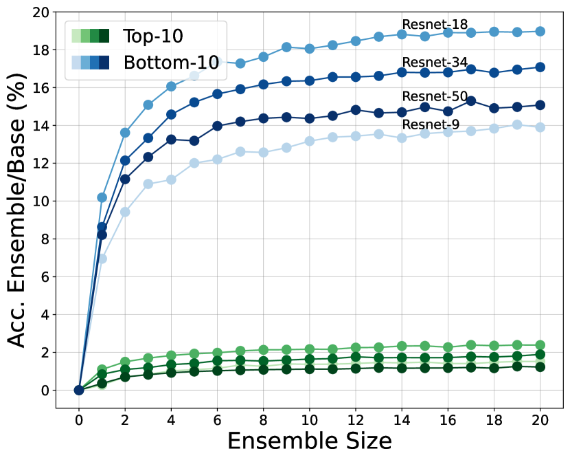
TinyImageNet

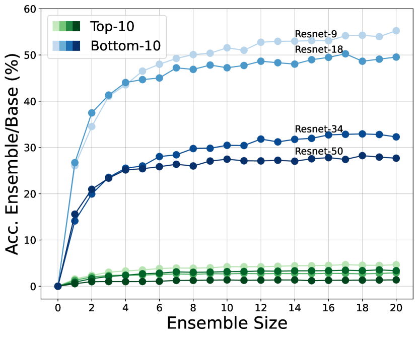
Figure 1: Relative Accuracy for Top-K/Bottom-K. Plot of the ratio of the homogeneous ensemble accuracy over a single base model (y-axis) illustrates strong benefits for the bottom-k group of ensembling while the top-k group only marginally benefits.

Understanding performance on subgroups is a frequent concern from a fairness perspective. A common fairness objective is mitigating disparate impact (Kleinberg et al., 2016; Zafar et al., 2015) where a class or subgroup of the dataset presents far higher error rates than other subsets of the distribution. In particular, and as we will thoroughly describe in section 2, many strategies have emerged to improve fairness by designing novel ensembling strategies based on fairness measures obtained from labeled attributes. In this study, we take a step back and focus on studying the fairness benefits of the simplest ensembling strategy: homogeneous ensembles. In this setting, the individual models in the ensemble all have the same architecture and hyperparameters. They are also trained with the same optimizer, data-augmentations, and training set.

Our results are surprising: despite the absence of "diversity" in the models being trained in the homogeneous ensemble, the only sources of randomness are (i) the parameters’ initialization, (ii) the realizations of the data-augmentations, and (iii) the ordering of the mini-batches. The final predictions are diverse enough to provide substantial improvements for both the minority groups and the bottom-k classes upon which a single model performs badly. This emergence of fairness is observed consistently across thousands of experiments on popular architectures (ResNet9/18/34/50, VGG16, MLPMixer, ViTs) and datasets (CIFAR10/100/100-C, TinyImagenet, CelebA) (section 3). The first important conclusion unlocked by our thorough empirical validation is that one may effectively improve minority group performance by using the same architecture and hyperparameters for each individual model without the need to observe corresponding labeled attributes. A second crucial finding is that solely controlling for initialization, batch ordering, and data-augmentation realizations is already enough to make training episodes produce models that are complementary with each other. Other factors such as architectures, optimizers, or data-augmentation families may not be the most important variables to produce fair ensemble (section 4). The last interesting observation is that, as a function of the number of models in the homogeneous ensemble, the average performance quickly plateaus after $4$ to $5$ models, but the bottom-k group performance keeps increasing steadily for up to $50$ models. In short, when performing deep ensembling, one should employ as many models as possible–even beyond the point at which the average performance plateaus–in order to produce a final ensemble with as much fairness as possible. Beyond fairness of homogeneous deep ensembles, our empirical study also offers a rich variety of new observations e.g., tying the severity of image corruption to the relative benefits that emerges from homogeneous deep ensembles.

Our contributions can be enumerated as follows:

1. We demonstrate that simple homogeneous deep ensembles trained with the same objective, architecture and optimization settings minimize worst-case error. This holds in both balanced and imbalanced datasets with protected attributes that the model is not trained on.

2. We further perform controlled sensitivity experiments where constructed class imbalance and data perturbation is applied (section 3). We observe that homogeneous ensembles continue to improve fairness and, in particular, the bottom-k group benefits more and more with the size of the ensemble compared to the top-k group as the severity of the corruption increases. These observations are held even when the protected attribute is imbalanced and underrepresented, such as in our CelebA experiments.

3. We further dive into possible causes for this emergence of fairness in homogeneous deep ensembles by measuring model disagreement (section 4.1) and by ablating for the different sources of randomness, e.g., weight-initialization (section 4.2). We obtain interesting results that suggest certain sources of stochasticity such as mini-batch ordering or data-augmentation realizations are enough to bring diversity into homogeneous ensembles.

The codebase to reproduce our results and figures is available here

2 Related Work

Deep ensembling of Deep Neural Networks (DNNs) is a popular method to improve top-line metrics (Lakshminarayanan et al., 2016). Several works have sought to further improve aggregate performance by amplifying differences between models in the ensemble ranging from varying the data augmentation used for each model (Stickland & Murray, 2020), the architecture (Zaidi et al., 2021), the hyperparameters (Wortsman et al., 2022), and even the training objectives (Jain et al., 2020). As will become clear, our focus is on the opposite setting where all the models in the ensemble share the same objective, training set, architecture, and optimizer.

Beyond Top-line metrics Discussions of algorithmic bias often focus on datasets collection and curation (Barocas et al., 2019; Zhao et al., 2017; Shankar et al., 2017), with limited work to-date understanding the role of model design or optimization choices on amplifying or curbing bias (Ogueji et al., 2022; Hooker et al., 2019; Balestriero et al., 2022). Consistent with this, there has been limited work to-date on understanding the implications of ensembling on subgroup error. (Grgić-Hlača et al., 2017) points out the theoretical possibility of using an ensemble of randomly selected candidate models to improve fairness, however no empirical validation was presented. (Bhaskaruni et al., 2019) considers AdaBoost (Freund & Schapire, 1995) ensembles and shows that upweighting unfairly predicted examples reaches higher fairness. (Kenfack et al., 2021; Chen et al., 2022) propose explicit schemes to induce fairness by designing heterogeneous ensembles, and (Gohar et al., 2023) provides ensemble design suggestions in heterogeneous ensembles. Recently, (Cooper et al., 2023) proposed a self-consistency metric for measuring the arbitrariness of single model outputs and provided a modified bagging solution specifically designed to mitigate the arbitrariness from model predictions. In contrast, our goal is to demonstrate how the simplest homogeneous ensembling strategy where each model is trained independently and with identical settings naturally exhibit fairness benefits without having to measure or have labels for the minority attributes.

Understanding why ensembling benefits subgroup performance. Several works to date have sought to understand why weight averaging performs well and improves top-line metrics (Gupta et al., 2022). However, few to our knowledge have sought to understand why ensembles disproportionately benefit bottom-k and minority group performance. In particular, (Rame et al., 2022) explores why weight averaging performs well on out-of-distribution data, relating variance to diversity shift. In this work, we instead explore how individual sources of inherent stochasticity in uniform homogeneous ensembles impact subgroup performance.

In this work, we consider the impact of ensembling on both balanced and imbalanced subgroups. Fairness considerations emerge for both groups. Real world data tends to be imbalanced, where infrequent events and minority groups are under-represented in the data collection processes. This leads to representational disparity (Hashimoto et al., 2018) where the under-represented group consequently experiences higher error rates. Even when training sets are balanced, with an equivalent number of training data points, certain features may be imbalanced leading to a long-tail within a balanced class. Both settings can result in disparate impact, where error rates for either a class or a subgroup are far higher (Chatterjee, 2020; Feldman & Zhang, 2020). This notion of unfairness is widely documented in machine learning systems: (Buolamwini & Gebru, 2018) find that facial analysis datasets reflect a preponderance of lighter-skinned subjects, with far higher model error rates for dark skinned women. (Shankar et al., 2017) show that models trained on datasets with limited geo-diversity show sharp degradation on data drawn from other locales. Word frequency co-occurrences within text datasets frequently reflect social biases relating to gender, race and disability (Garg et al., 2017; Zhao et al., 2018; Bolukbasi et al., 2016; Basta et al., 2019).

In the following section 3, we will study how the randomness stemming from the random initialization, data-augmentation realization, or mini-batch ordering during training may provide enough diversity in homogeneous deep ensembles for fairness to naturally emerge. The why is left for section 4.

ensemble/base

ResNet9

  models in ensemble

ResNet18

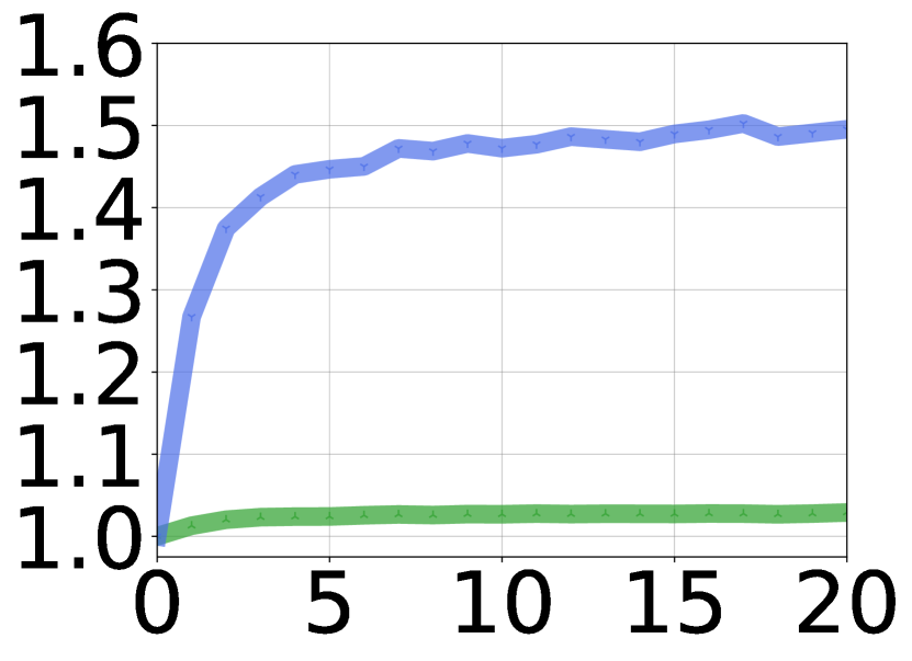
  models in ensemble

ResNet34

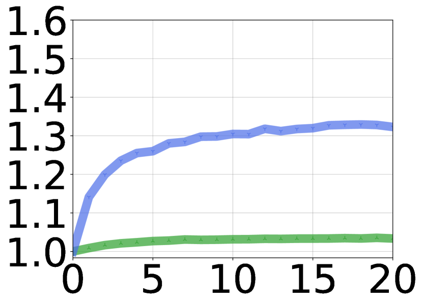
  models in ensemble

ResNet50

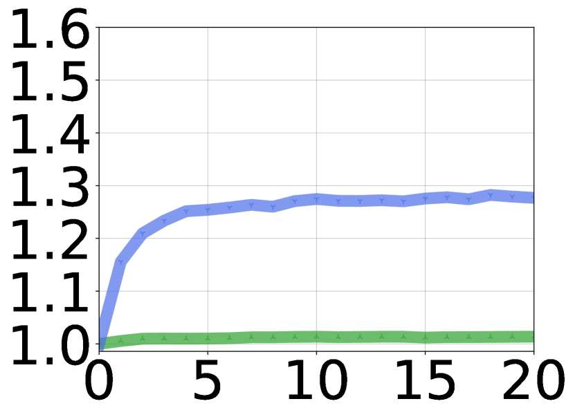
  models in ensemble

VGG16

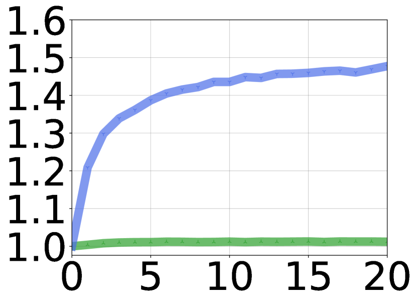
  models in ensemble

ViT

  models in ensemble

Figure 2: Test set accuracy gain as a ratio of ensemble accuracy % over the singular base model (y-axis) by group (top-k and bottom-k) for TinyImageNet for different architectures (columns) with varying the number of models within the homogeneous ensemble grows (x-axis). We clearly observe that as the number of models within the homogeneous ensemble grows, the bottom-k group performance improves. In particular, the bottom-k group’s accuracy gain outgrow the top-k group’s. This occurs despite the fact that the models within the ensemble are all employing the same hyperparameters, thus inherently share the same functional biases. The absolute accuracies are provided in table 1 below, and CIFAR100 results are in fig. 8.

3 FAIR-Ensemble: When Homogeneous Ensembles Disproportionately Benefit Minority Groups

Throughout our study, we will consider a DNN to be a mapping $f_{\theta}:\mathcal{X}\mapsto\mathcal{Y}$ with trainable weights $\theta\in\Theta$. The training dataset $\mathcal{D}$ consists of $N$ data points $\mathcal{D}=\left\{\mathbf{x}_{n},y_{n}\right\}_{n=1}^{N}$. Given the training dataset $\mathcal{D}$, the trainable weights are optimized by minimizing an objective function. We denote a homogeneous ensemble of $m$ classification models by $\left\{{f_{\theta}}_{1},\ldots,{f_{\theta}}_{m}\right\}$, where ${f_{\theta}}_{i}$ is the $i^{th}$ model. Each model is trained independently of the others. We will denote by homogeneous ensemble the setting where the same model architecture, hyperparameters, optimizer, and training set are employed for each model of the ensemble.

3.1 Experimental Set-up

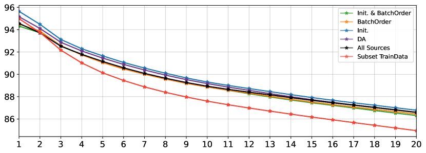
K size

(a) ResNet-50 Top-K classes

test accuracy %

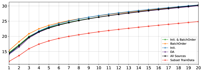
K size

(b) ResNet-50 Bottom-K classes

Figure 9: Average Top and Bottom-K accuracy as number of K-classes increase. We observe that DA and Init. outperforms All Sources baseline performance in Top-K classes, whereas BatchOrder and Init. outperfroms All Sources on Bottom-K classes. In both top and bottom groups, only the TrainSubsetData variant underperforms All Sources.

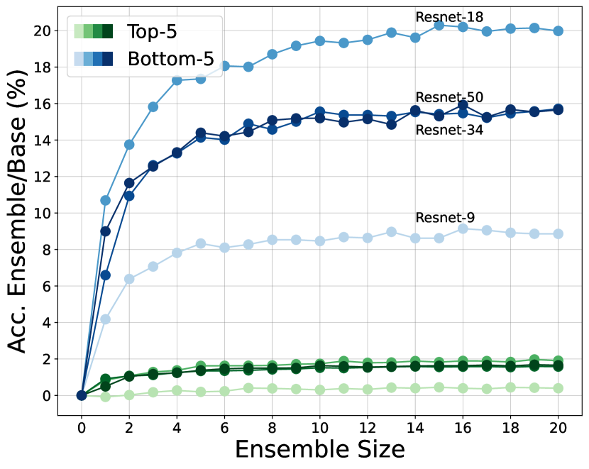
K=10

K=20

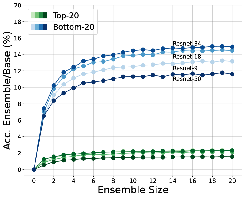
Figure 14: Top/Bottom-K performance for K = {5,10,20} in CIFAR100

Experimental set-up: we evaluate homogeneous ensembles on CIFAR100 (Krizhevsky et al., 2009) and TinyImageNet (Russakovsky et al., 2015) datasets across various architectures: ResNet9/18/34/50 (He et al., 2016a), VGG16 (Simonyan & Zisserman, 2014), MLP-Mixer (Tolstikhin et al., 2021) and ViT (Dosovitskiy et al., 2020). Training and implementation details are provided in appendix A. Whenever we report results on the homogeneous ensemble, unless the number of models is explicitly stated, it will comprise of 20 models. Each model is trained independently as in(Breiman, 2001; Lee et al., 2015), i.e. we do not control for any of the remaining sources of randomness as this will be explored exclusively within section 4.2.
Balanced Dataset Sub-Groups: for top-k and bottom-k, we calculate the class accuracy of the base model and find the best and worst $K$ ($K=10$) performing classes and track the associated classes as bottom-k and top-k groups. We then proceed to measure how performance on these groups changes as a function of the homogeneous ensemble size. We highlight that although we leverage $K=10$ in many experiments, the precise choice of $K$ does not impact our findings, as demonstrated in fig. 9 and fig. 14.
Imbalanced Dataset Sub-Groups: we consider a setting where the protected attribute is an underlying variable different from the classification target. Similar to the setup in (Hooker et al., 2019; Veldanda et al., 2022), we treat CelebA(Liu et al., 2015) as a binary classification problem where the task is predicting hair color $\mathcal{Y}$ ={blonde, dark haired} and the sensitive attribute is gender. In this dataset, blonde individuals constitute only 15% of which a mere 6% are males. Hence, blonde male is an underrepresented attribute. We then proceed to measure how performance on the protected gender:male attribute varies as a function of ensemble size.

Given the above experimental details, we can now proceed to present our core observations that tie the homogeneous ensemble size with its fairness benefits.

3.2 Observing Disproportionate Benefits For Bottom-K Groups

CIFAR100
ensemble/base ResNet9
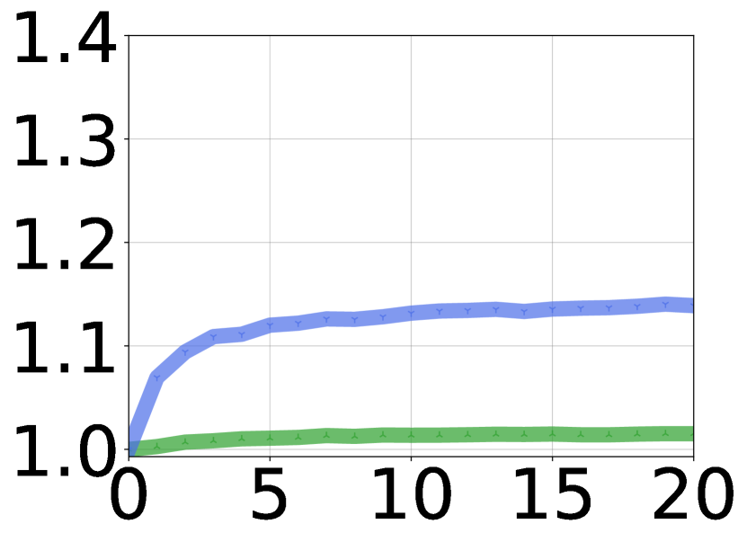
ResNet18
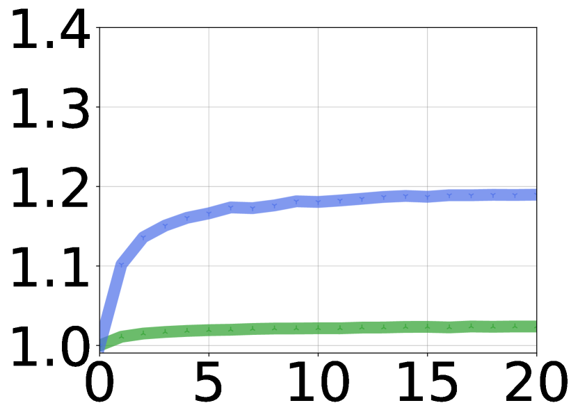
ResNet34
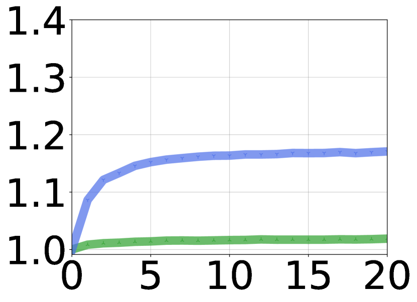
ResNet50
VGG16
MLP-Mixer

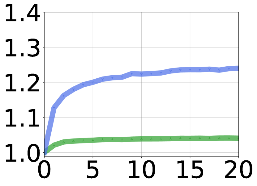
Figure 8: Depiction of the accuracy gain as a ratio of ensemble accuracy % over the singular base model (y-axis) by per-group (top-k and bottom-k) test set accuracies for CIFAR100.

Table 1: Depiction of the average and per-group (top-k and bottom-k) absolute test set accuracies corresponding to the models and datasets depicted in fig. 2 above and fig. 8 in the Appendix, again the homogeneous ensemble consists of $20$ models. We clearly observe that fairness naturally emerges through ensembling i.e. the bottom-k group substantially benefits from homogeneous ensembling compared to the top-k group.

	CIFAR100						TinyImageNet
	Ensemble			Single			Ensemble			Single
Arch.	mean	top-k	bottom-k	mean	top-k	bottom-k	mean	top-k	bottom-k	mean	top-k	bottom-k
ResNet9	77.01	92.18	58.43	72.21	90.80	51.30	58.29	86.66	23.60	50.71	82.80	15.20
ResNet18	78.15	94.19	59.13	73.57	92.00	49.70	56.50	86.64	24.82	49.29	84.20	16.60
ResNet34	78.68	93.84	58.89	74.26	92.10	50.30	58.89	87.44	27.25	52.18	84.60	20.60
ResNet50	77.94	93.53	58.34	74.88	92.40	50.70	60.35	87.38	28.09	55.00	86.20	22.00
VGG16	76.95	92.88	57.32	71.24	91.50	44.40	67.04	90.27	38.71	60.36	89.20	26.20
MLPMixer/ViT	66.69	87.95	40.93	60.25	84.50	33.00	56.97	85.60	22.42	51.23	84.20	17.20

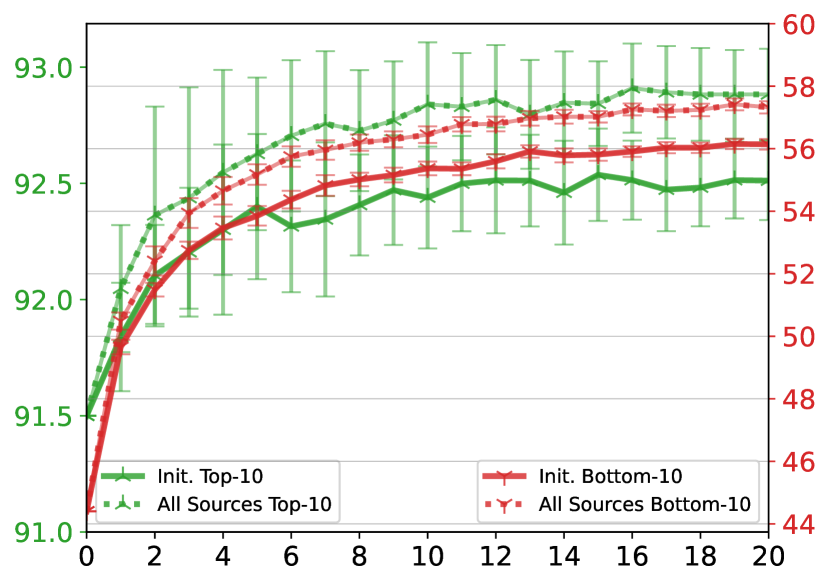
BatchOrder

DA

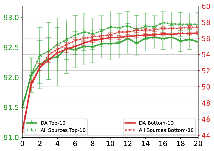
Init & BatchOrder

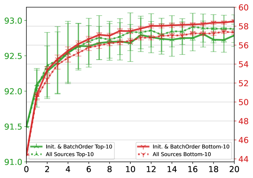
MLP-Mixer
ensemble/base Init

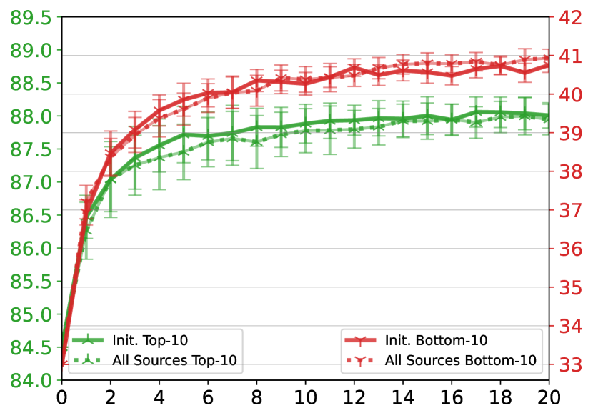
   models in ensemble BatchOrder

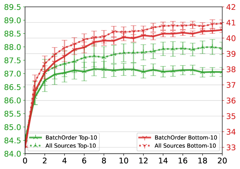
   models in ensemble DA

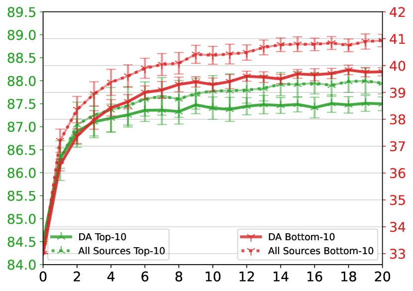
   models in ensemble Init & BatchOrder

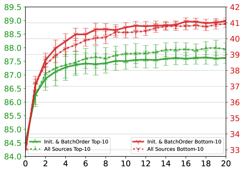
   models in ensemble

Figure 11: Accuracy for Top-K and Bottom-K across models added to ensemble on CIFAR100

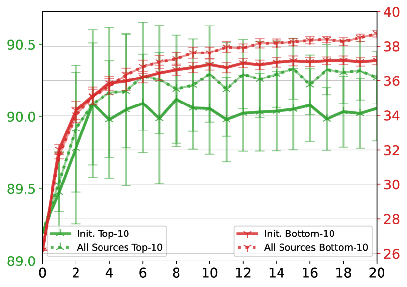
BatchOrder

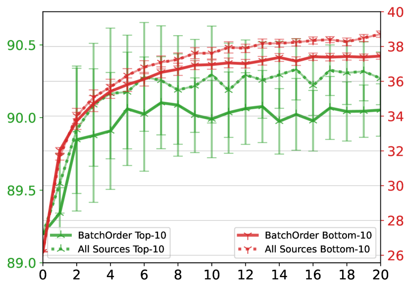
DA

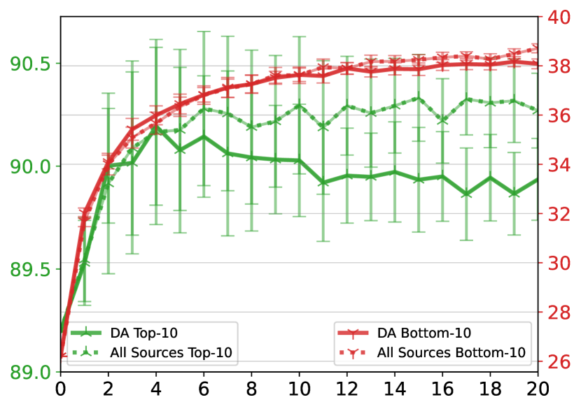
Init & BatchOrder

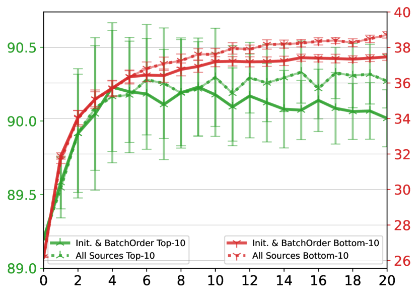
ViT

ensemble/base

Init

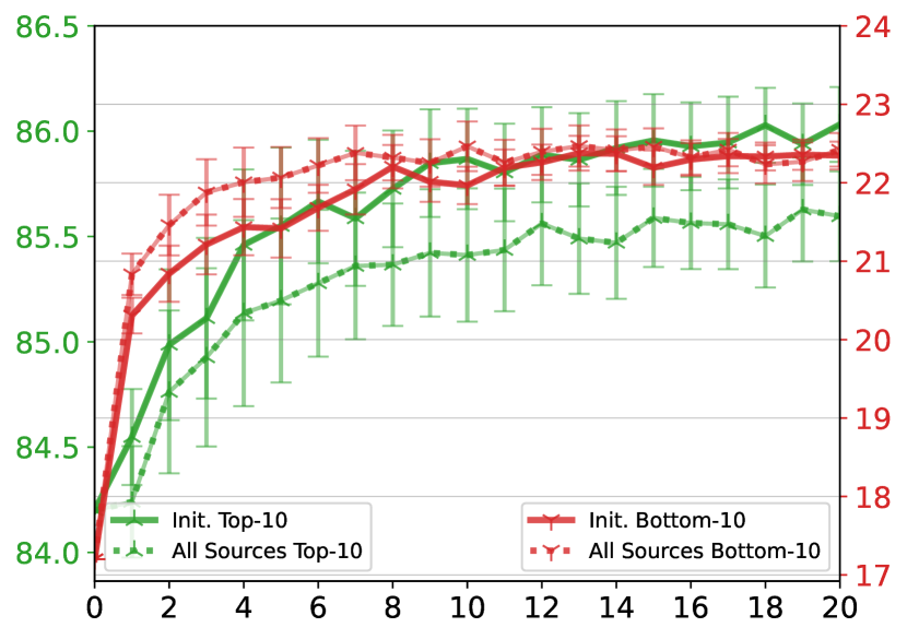
   models in ensemble

BatchOrder

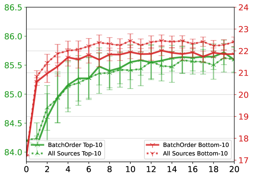
   models in ensemble

DA

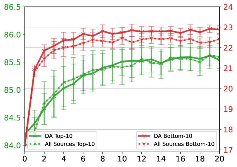
   models in ensemble

Init & BatchOrder

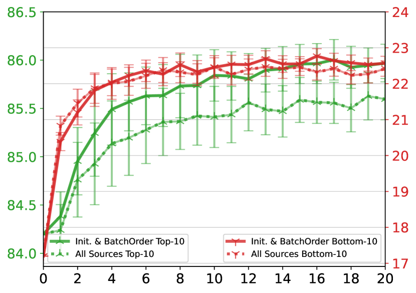
   models in ensemble

Figure 13: Accuracy for Top-K and Bottom-K across models added to ensemble on TinyImageNet

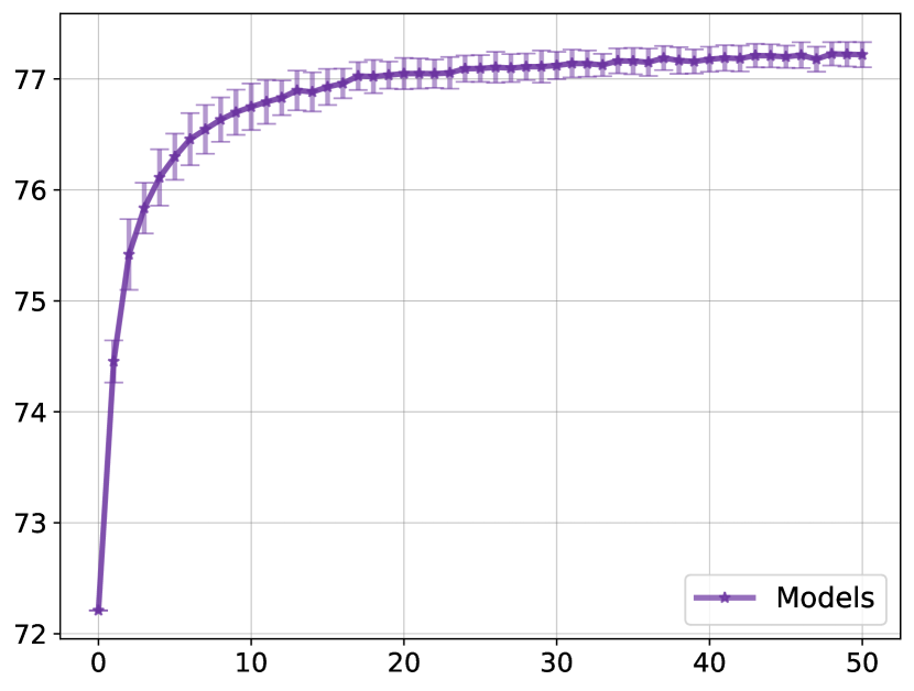
models in ensemble

(a) ResNet9 on CIFAR100

test accuracy %

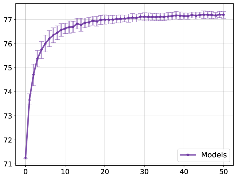
models in ensemble

(b) VGG16 on CIFAR100

test accuracy %

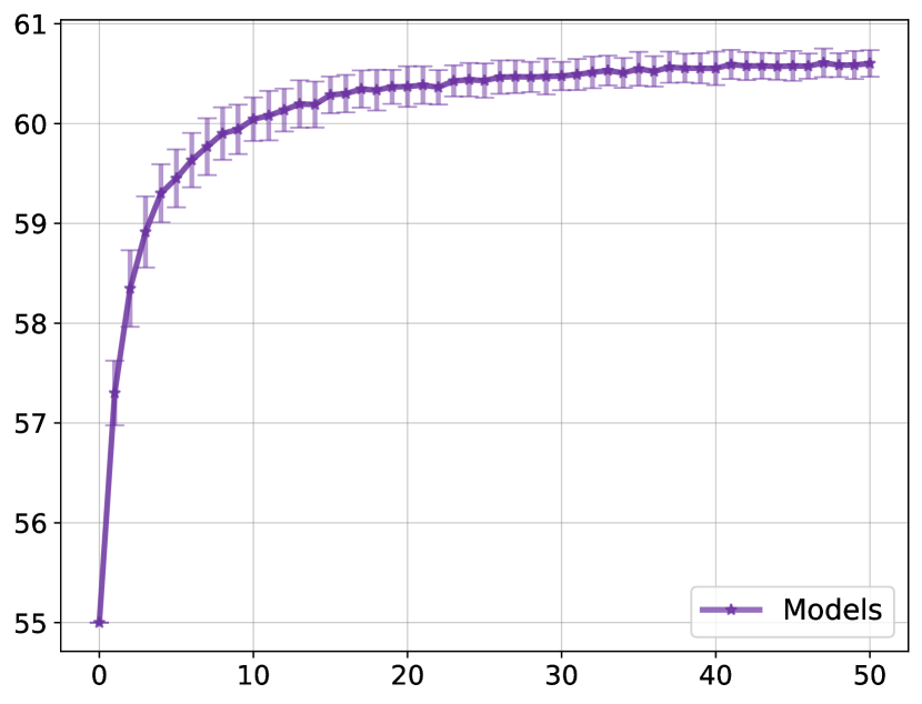
models in ensemble

(c) ResNet50 on TinyImageNet

Figure 20: Average Accuracy per size of homogeneous ensemble. The average accuracy for each model added is calculated by averaging 100 random samples from a population of 50 models. We can see that the average accuracy starts to slowly plateau as the ensemble grows to 50 models.

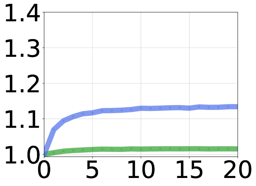
DA

Init & BatchOrder

All Sources

Resent9 50 model ensemble

ensemble/base

Init

BatchOrder

DA

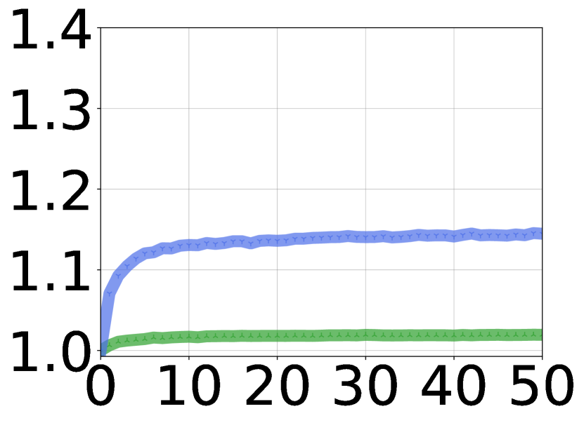
Init & BatchOrder

All Sources

VGG16 20 model ensemble

ensemble/base

Init

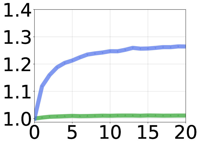
BatchOrder

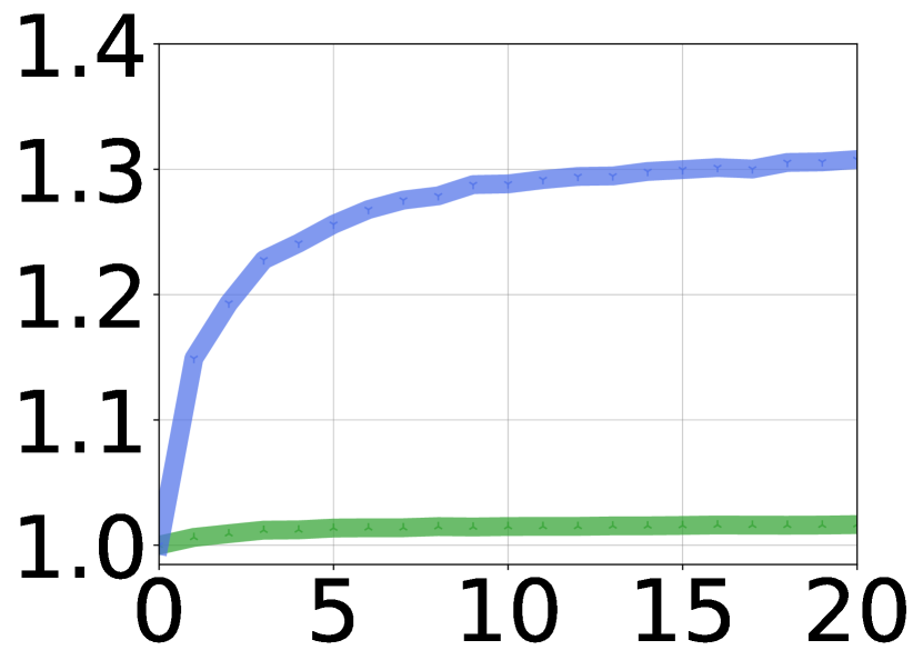
DA

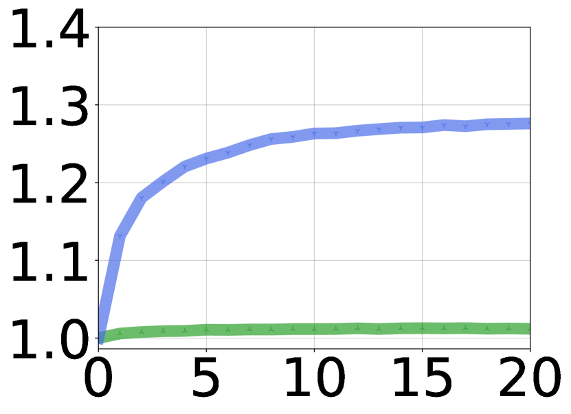
Init & BatchOrder

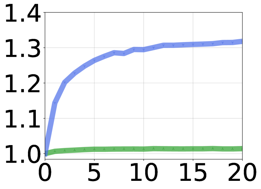
All Sources

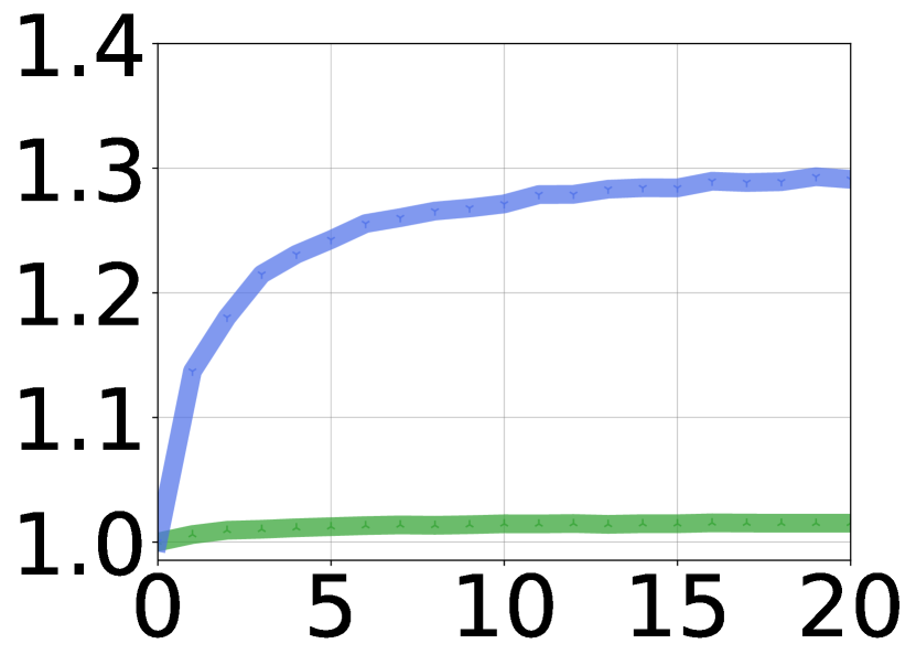
VGG16 50 model ensemble
ensemble/base Init
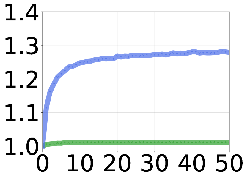
BatchOrder
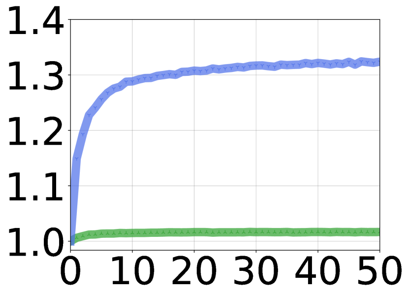
DA
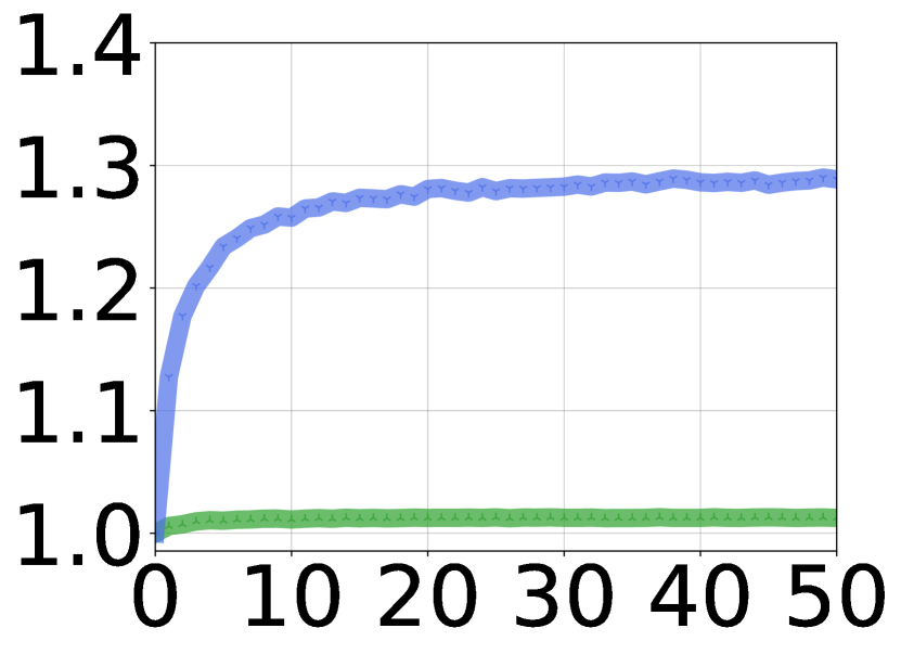
Init & BatchOrder
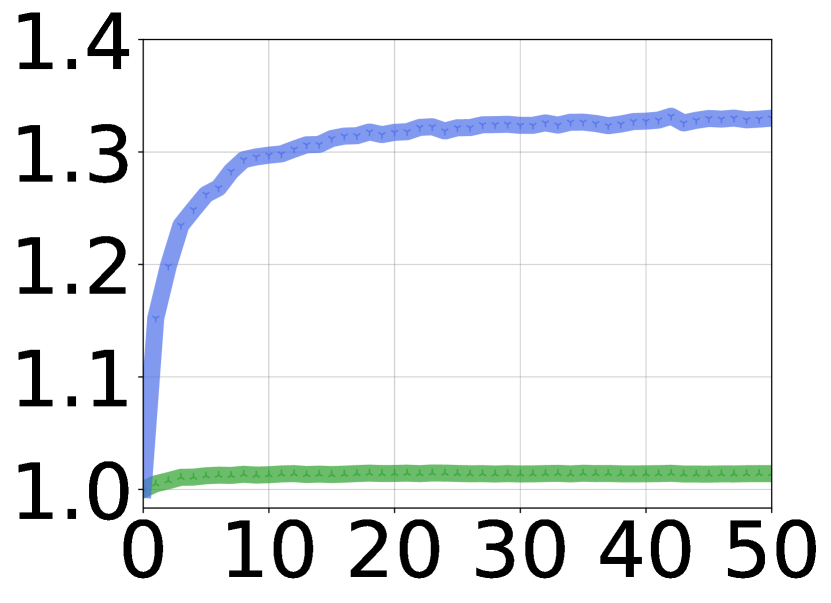
All Sources

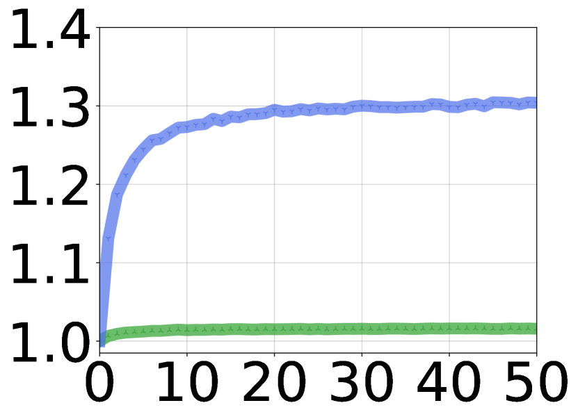
MLP-Mixer 20 model ensemble
ensemble/base Init

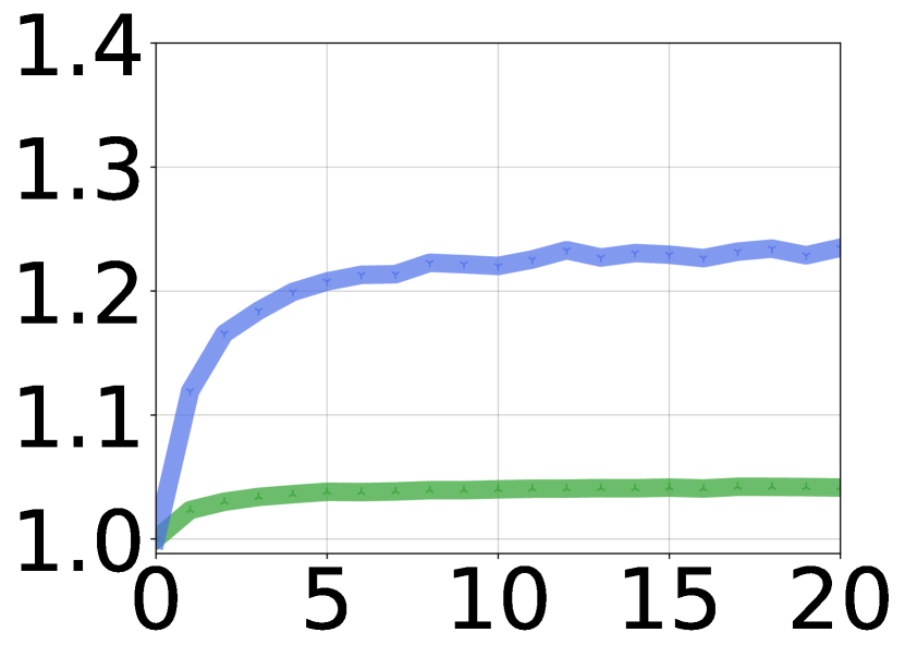
   models in ensemble BatchOrder

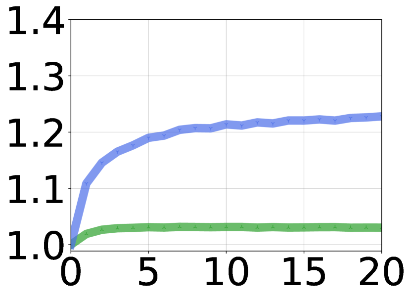
   models in ensemble DA

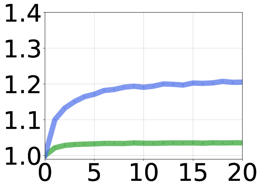
   models in ensemble Init & BatchOrder

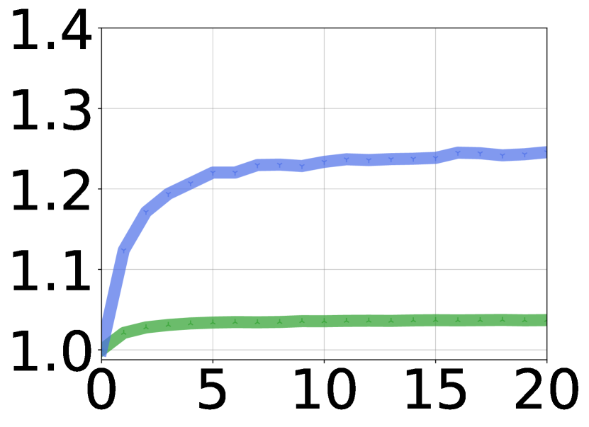
   models in ensemble All Sources

   models in ensemble

Figure 21: Ratio of Top & Bottom K ensemble accuracy for different model architectures and ensemble sizes on CIFAR100

Impact on bottom-k classes: in fig. 1 and fig. 2, we plot the relative gain in accuracy, i.e., the ratio between the homogeneous ensemble and base model performance on top-k/bottom-k groups, for each model architecture and dataset. Therefore answering the question: what is the relative improvement in performance of using a homogeneous ensemble over a single model? Across models and datasets, there is a disproportionate benefit for the bottom-k performance. For CIFAR100, this benefit ranges from 14%-29% for bottom-k across different architectures compared to 1%-4% for top-k. For TinyImageNet the benefits are even more pronounced with a maximum gain of 55% for bottom-k compared to 5% for top-k across different architectures. We also provide in table 1 the absolute per-group accuracy and average performances for the corresponding models and datasets. For example, we observe a gain of more than 10% in absolute accuracy for the bottom-k classes against a gain of around 4% for the top-k group across settings. As a result, we obtain that even when ensembling models that share all their hyperparameters, data, and training settings, fairness naturally emerges. Given these observations, one may wonder how does the number of models in the homogeneous ensemble impact fairness benefits. In fig. 2 and fig. 8, we plot fairness impact as a function of $m$, the number of models being used. A key observation we obtain is that while the top-k group’s performance plateaus rapidly for small $m$, the bottom-k group still exhibits improvements when reaching $m=20$. We further explore increases of $m$ in the Appendix, where we consider up to 50 model ensembles (see fig. 20). In both TinyImageNet and CIFAR100 datasets, the absolute accuracy improvements of architectures such as ResNet9, ResNet50, and VGG16 all slowly plateaued as $m\rightarrow 50$; we also present the relative test set accuracies in figs. 21 and 23. For the test set accuracy performance between the top-k and the bottom-k groups over ensemble size and associated absolute errors, please refer to fig. 11 and fig. 13.

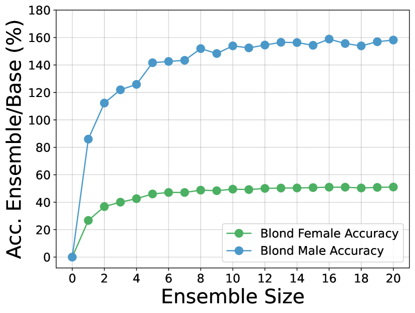
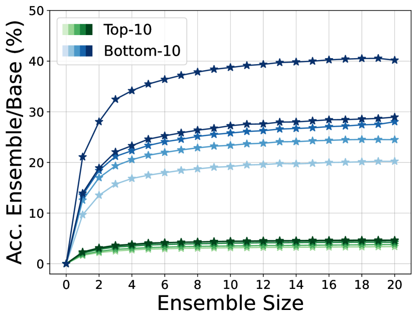
Figure 3: Left: CelebA test set accuracy gain as a ratio of ensemble accuracy % over the singular base model (y-axis) by group (majority and minority). Male is the protected attribute and Blond Males are extremely underrepresented in the training data. Nevertheless, we clearly observe that as the number of models within the homogeneous ensemble grows (x-axis), the protected attribute group’s classification accuracy outgrows the majority group’s. Right: CIFAR100-C test set accuracy gain ratio (same as left per-group top-k and bottom-k) of the homogeneous ensemble as the number of models being aggregated increases (x-axis) for varying severity of corruption levels in CIFAR100-C (recall fig. 24) from light to dark color shading. A striking observation is that not only does homogeneous DNN ensembling improves fairness by increasing the performance on the bottom group more drastically than on the top group, this effect is even more prominent at higher corruption severity levels.

Controlled Experiment: CelebA Beyond looking at the top-k and bottom-k classes, we leverage the CelebA dataset which contains fine-grained attributes to study the fairness impact of homogeneous ensembles. Using the ResNet18 architecture, we train $20$ models and measure their performances on the protected gender:male attribute. Employing homogeneous ensembles, we observe the average performance for the Blonde classification task to increase from 92.02% to 94.04%. Furthermore, for the protected gender attribute, we see the average performance increase from 9.44% to 21.80%, a considerable benefit that alleviates the disparate impact on an under-represented attribute. As we previously observed, homogeneous ensembles provide a disproportionate accuracy gain in the minority subgroup as further depicted in figs. 3 and 7.

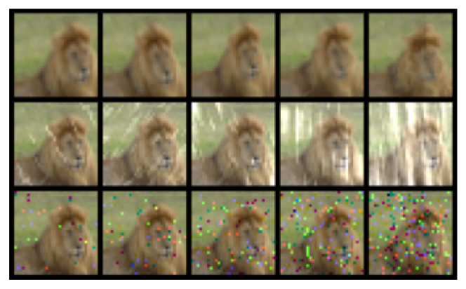
Figure 24: For each row we depict three of the different types of corruptions from the CIFAR100-C dataset (elastic_transform, snow, and impulse_noise respectively), and for each column we depict the corruption severity levels ($1\mapsto 5$). The image belongs to the lion class.

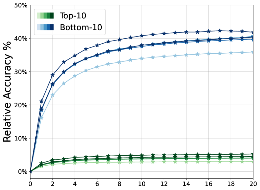
models in ensemble

(b) VGG-16

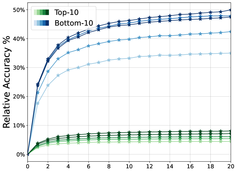
models in ensemble

(c) MLP-Mixer

Figure 25: Performance on CIFAR-100 Corrupt based on Severity Levels.

Controlled Experiment: CIFAR100-C (Hendrycks & Dietterich, 2018) is an artificially constructed dataset of 19 individual corruptions on the CIFAR100 Test Dataset as depicted in fig. 24, each with a severity level ranging from 1 to 5. Our goal is to understand the relation between fairness benefits for the bottom-k group and severity of the input corruption. We thus propose to benchmark our homogeneous ensembles on all severity levels, and for completeness, we benchmark and average performance across all corruptions for each severity level. In fig. 3, we depict the gain in test-set accuracy achieved by the top-k and bottom-k (K=10) classes as the ensemble size ($m$) increases relative to a single model. We see that, consistent with earlier results, gains on top-k plateau earlier as the size of the ensemble increases. However, the benefits of homogeneous ensembles are even more pronounced when the data is increasingly corrupted. We observe in fig. 25 that the largest fairness benefits occur with the maximum severity, with a maximum relative gain of 40.17% for severity 5 vs 20.18% for severity 1.

CIFAR100

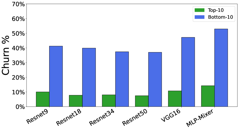
TinyImageNet

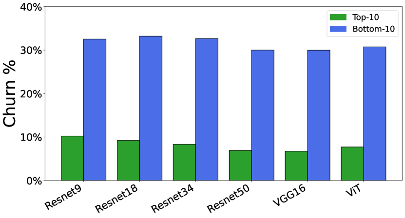
Figure 4: Depiction of churn results across models and datasets. The results demonstrate that churn is significantly higher for the bottom-k group compared to the top-k group, indicating that ensembling these models disproportionately impacts the bottom-k group (as defined in eq. 1). The difference in churn between bottom-k and top-k groups varies based on model architecture, suggesting that some homogeneous ensembles achieve more fairness than others.

4 Why Homogeneous Ensembles Improve Fairness

We established in the previous section 3 that homogeneous ensembles overly benefit minority sub-group performance. However, it is still unclear why. In this section, we take a step towards understanding that effect through the scope of model disagreement, and in particular how the only three sources of stochasticity in homogeneous ensemble may impact those results.

4.1 Difference in Churn Between Models Explains Ensemble Fairness

It might not be clear a priori how to explain the disparate impact of homogeneous deep ensembling in bottom-k groups compared to top-k groups, as we observed in the previous section 3, however we do know that such benefit only appears if the individual models do not all predict the same class, i.e., there is disagreement between models. One popular metric of model disagreement known as the churn will provide us with an obvious yet quantifiable answer.

Experiment set-up. To understand the benefit of model ensembling one has to recall that if all the models within the ensemble agree, then there will not be any benefit to aggregating the individual predictions. Hence, model disagreement is a key metric that will explain the stark change in performance that our homogeneous DNN ensembles have shown on the bottom-k group. We consider differences in churn between top-k and bottom-k. We also recall that the predictive churn is a measure of predictive divergence between two models. There are several different proposed definitions of predictive churn (Chen et al., 2020; Shamir & Coviello, 2020; Snapp & Shamir, 2021); we will employ the one that is defined on two models $f_{1}$ and $f_{2}$ as done by (Milani Fard et al., 2016) as the fraction of test examples for which the two models disagree:

$$C(f_{1},f_{2}) =\mathbb{E}_{\mathcal{X}}\big{[}\mathbbm{1}_{\{\hat{\mathcal{Y}}_{x;f_{1}}\neq\hat{\mathcal{Y}}_{x;f_{2}}\}}\big{]},$$ (1)

where $\mathbbm{1}$ is the indicator. For an ensemble with more than two models, we will report the average churn computed across $100$ randomly sampled (without replacement) pairs of models. As a further motivation to employ eq. 1, we provide in appendix F the strong correlation between Churn(%) and Test accuracy improvement(%) for various architectures on both CIFAR100 and TinyImageNet. In fact, the Pearson correlation coefficient (a maximum score of 1 indicates perfect positive correlation) between churn and test set accuracy are $0.975$ for CIFAR100 and $0.93$ for TinyImageNet i.e., a greater value for eq. 1 is an informative proxy on the impact toward test set accuracy.

Observations.  In fig. 4, we report churn for various architectures on CIFAR100 and TinyImagenet. We observe that architectures differ in the overall level of churn, but a consistent observation across architectures emerges: there are large gaps in the level of churn between top-k and bottom-k. For example, on ResNet18 for TinyImageNet the difference is churn of 9.22% and 33.21% for top-k and bottom-k respectively, while it is 7.78% and 39.89% for top-k and bottom-k for CIFAR100. In short, the models disagree much more when looking at samples belonging to the bottom-k groups than when looking at samples belonging to the top-k groups. In fact, when looking at the samples of the bottom-k classes, the models vary in which samples are incorrectly classified (by definition of churn, please see eq. 1). As a result, that group benefits much more from homogeneous ensembling. From these observations, it becomes clear that poor performance from individual models on the bottom-k subgroups does not stem from a systemic failure and can thus be overcome through homogeneous ensembling.

test accuracy %

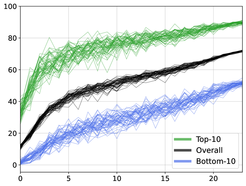
(a) Batch Order

epochs

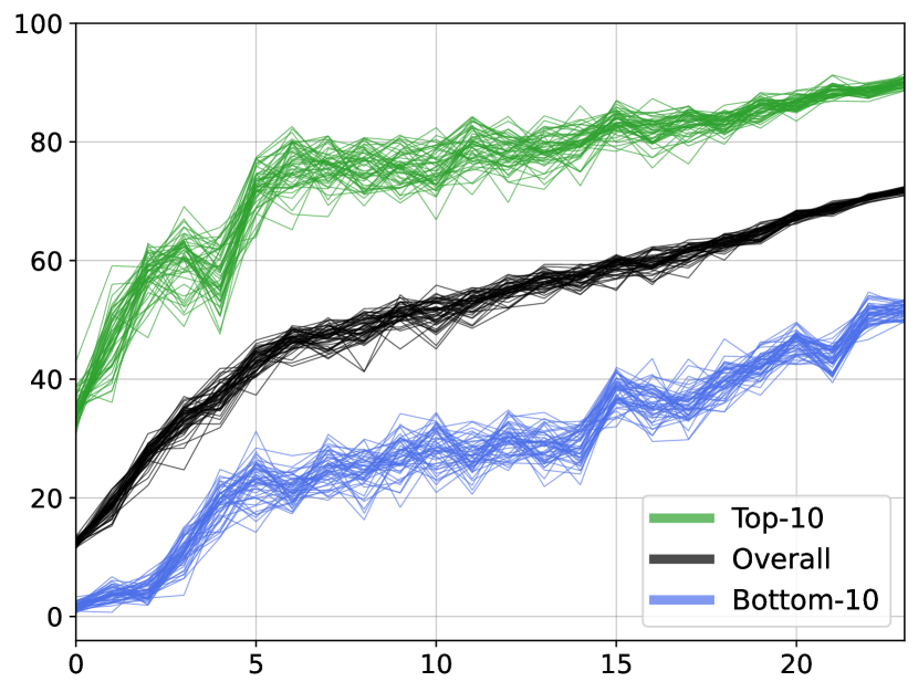
(b) Data-Augmentation

epochs

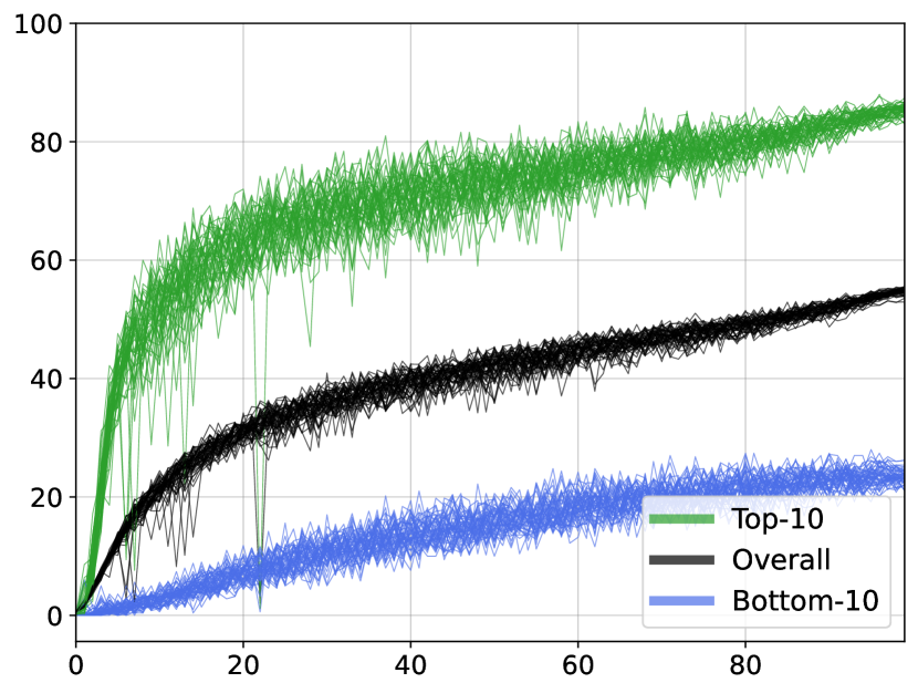
(c) Batch Order

epochs

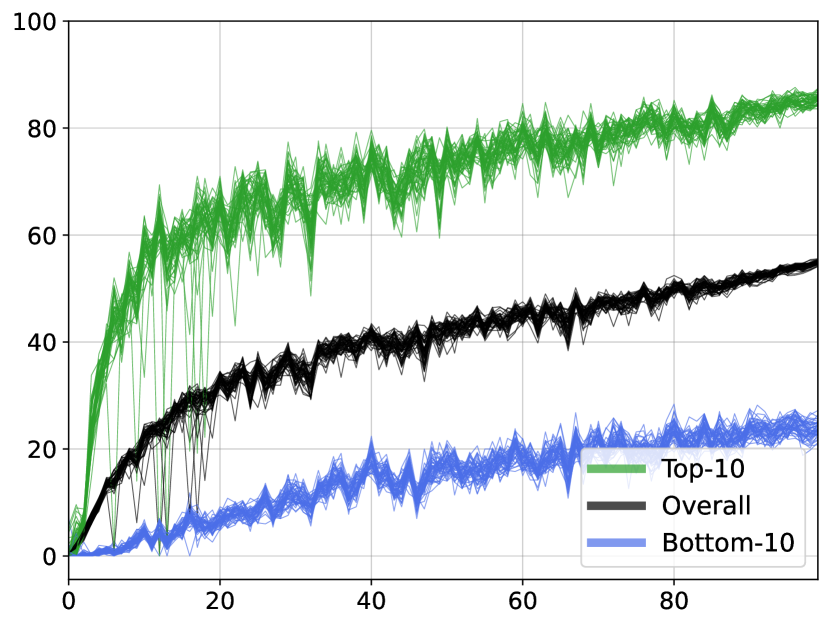
(d) Model Initialization

epochs

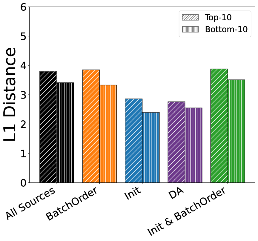
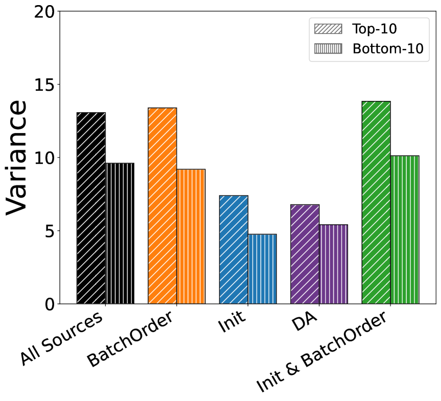
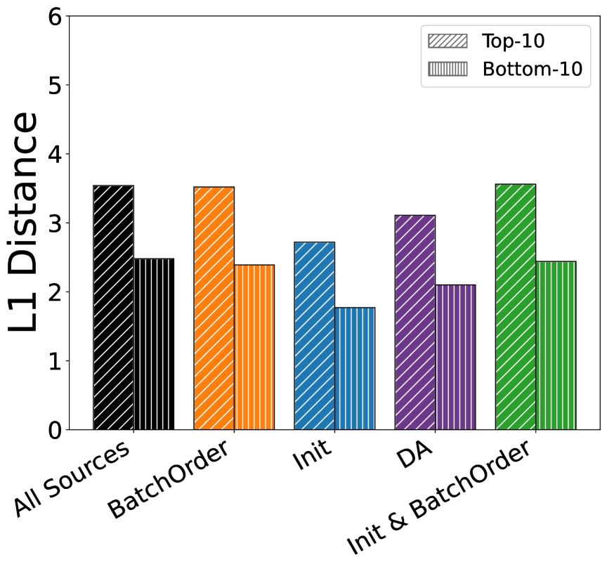
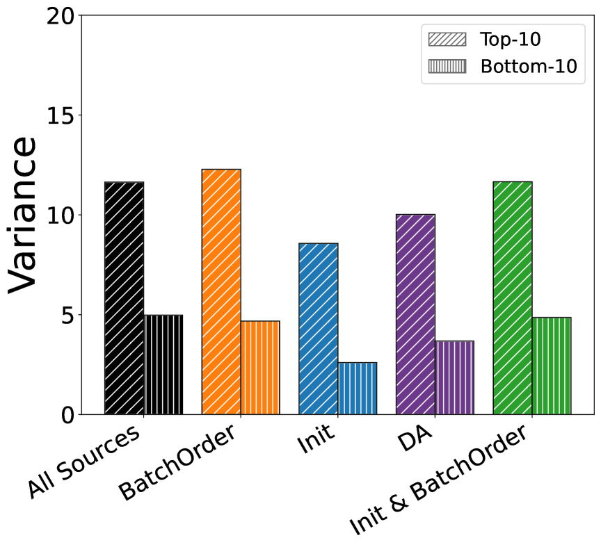
Figure 5: Depiction of multiple individual training episodes of a ResNet9 model on CIFAR100 (two left columns) and ResNet50 model on TinyImageNet (two right columns). We clearly observe that varying one factor of stochasticity at a time highlights which ones provide the most randomness between training episodes. In this setting, we see that batch ordering is the main source. On the other hand, model-init and data-augmentation have little effect and we even observe very similar trends at different epochs between the individual runs.

4.2 Characterizing Stochasticity In Deep Neural Networks Training

While section 3 demonstrated the fairness benefits of homogeneous ensembles, and section 4.1 linked those improvements to increased disagreement between the individual models for the minority group and bottom-k classes, one question remains unanswered: what drives models trained with the same hyperparameters, optimizers, architectures, and training data to end-up disagreeing? This is what we propose to answer in this section by controlling each of the possible sources of randomness that impact training of the individual models.

% accuracy diff.

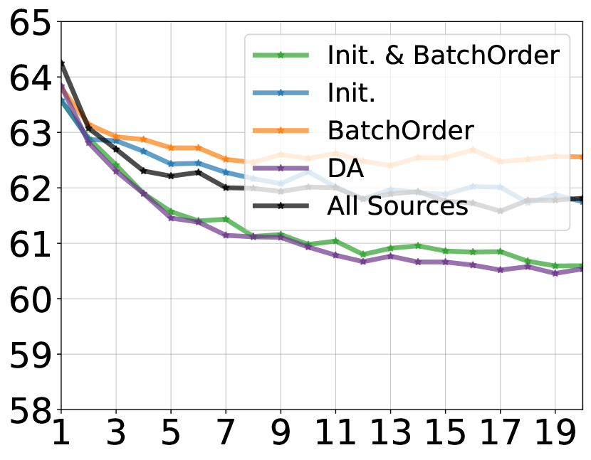
models in ensemble

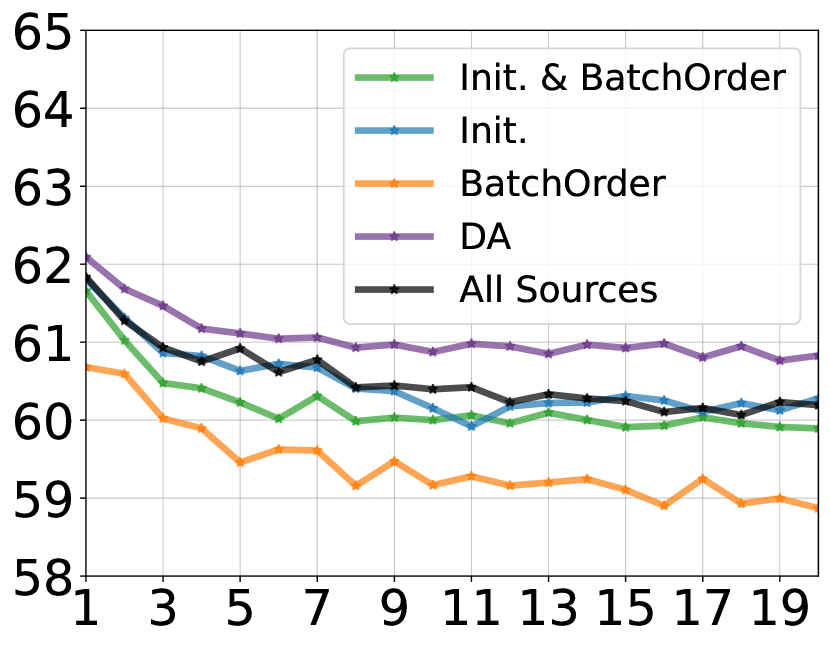
models in ensemble

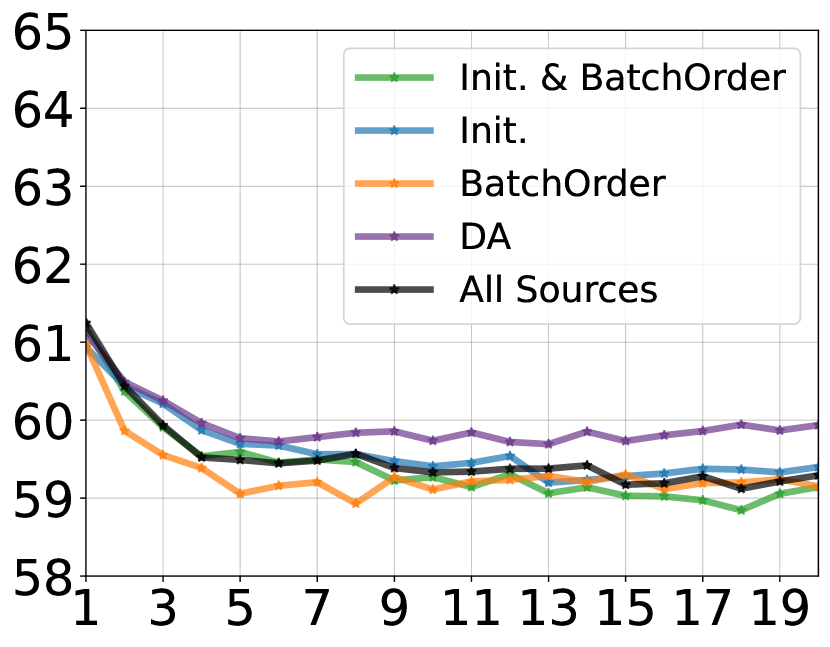
models in ensemble

Figure 6: Accuracy % difference between top and bottom 10 classes, for ResNet18 (left), 34 (middle), and 50 (right) for TinyImageNet. We clearly observe that once we control for the different sources of stochasticity, it is possible to skew the ensemble to favor the bottom group, in which case fairness is further amplified compared to the baseline ensemble. Although the trends seem mostly consistent across architectures of the same family (ResNets) and datasets, it is not necessarily the case between architecture families: see fig. 15 for ResNet-CIFAR100, fig. 18 for MLPMixer/VGG16-CIFAR100 andViT/VGG16-TinyImagenet.

To understand more what introduces the most significant levels of stochasticity, we first explore how different sources of randomness impact the training trajectories of DNNs. In particular, for homogeneous ensembles there are only three source of randomness: (i) Random Initialization (Glorot & Bengio, 2010; He et al., 2016b), (ii) Data augmentation realizations (Kukačka et al., 2017; Hernández-García & König, 2018), and (iii) Data shuffling and ordering (Smith et al., 2018; Shumailov et al., 2021). Clearly, if a source introduces low randomness, different training episodes will produce models with low disagreement and thus low fairness benefits.

Experiment set-up. To isolate the impact of the different sources of stochasticity, we propose an thorough ablation study of the following sources: Change Model Initialization (Init): for this ablation, we change the model initialization weights by changing the torch seed for each model before the model is instantiated. Change Batch Ordering (BatchOrder): for this ablation, we change the ordering of image data in each mini-batch by changing the seed for the dataloader for each model training. Change Model Initialization and Batch Ordering (Init & BatchOrder): for this ablation, both the model initialization and batch ordering are changed for each model training. Change Data Augmentation (DA): for this ablation, only the randomness in the data augmentation (e.g. probability of random flips, probability of CutMix(Yun et al., 2019), etc.) is changed. The relevant torch and numpy seeds are changed right before instantiating the data augmentation pipeline. Custom fixed-seed data augmentations is also used. Change Model Initialization, Batch Ordering and Data Augmentation (All Sources): for this ablation, the model initialization, batch ordering and data augmentation seeds are changed for each model training–this ablation represents the standard homogeneous ensemble of section 3. A last source of randomness can emerge from hardware or software choices and round-off errors (Zhuang et al., 2022; Shallue et al., 2019) which we found to be negligible compared to the others. In addition to providing training curves evolution for each ablation, we also use two quantitative metrics. First, we will leverage the L1-Distance of the accuracy trajectories during training, which is calculated for every epoch by averaging the absolute distance in accuracy among the ensemble members and averaging these values across the training epochs. Second, we will leverage the Variance of the different training episodes’ accuracy at each epoch and then average over all the epochs.

Observations. In fig. 5, we plot these measures of stochasticity for both CIFAR100 and TinyImageNet on different DNNs. We observe that the single sources of noise dominate, such that the ablations themselves equate to the level of noise in the DNN with all sources of noise present. In particular, we observe one striking phenomenon: the variation of the data ordering within each epoch between training trajectories BatchOrder is the main source of randomness. It is equivalent to the level of noise we observe for the DNN with all sources of noise All Sources, and the DNN with the ablation Init & BatchOrder. As seen in fig. 5 when the batch ordering is kept the same across training episodes, varying the data-augmentation and/or the model initialization has very little impact.

CelebA : Blonde

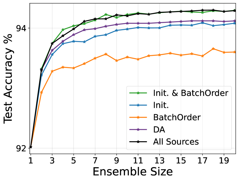
CelebA : Blonde Male

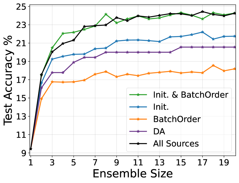
Figure 7: 20 Model Ensemble Performance (ResNet18) on Blond (left) and Blond Male (right) Classification in CelebA. In the overall blond classification, the max accuracy increased up to 2.27% using homogeneous ensembling, whereas for the Blond Male minority group the max accuracy increased dramatically–up to 14.99%–in the same ensembles.

4.3 Can Different Sources of Stochasticity Improve Homogeneous Deep Ensemble Fairness?

The last important point that needs to be addressed is to relate the amount of randomness that each of the three sources introduce (recall section 4.2) with the actual fairness benefits of the homogeneous ensemble. In fact, fig. 5 did emphasize how each source of randomness provides different training dynamics and levels of disagreements, which are the cause of the final fairness outcomes.

In fig. 6, we depict the accuracy difference between average top-k and bottom-k. A value of $0$ indicates that the model performs equally on both top-k and bottom-k classes. We observe that for the majority of dataset/architecture combinations, batch ordering minimizes the gap between top and bottom-k class accuracy. Surprisingly, the resulting fairness level is even greater than when employing all the source of stochasticity, i.e., it is possible to further improve the emergence of fairness in homogeneous ensembles solely by varying the batch ordering between the individual models. In fig. 7, we observe that although gains quickly plateau for the Blonde category in all sources, the stochasticity introduced by initialization and batch ordering Init & BatchOrder matches, and sometimes outperforms the noise ablation on the minority group performance. There is one exception to this, as we see that data-augmentation variation for ResNet18 on TinyImageNet creates the largest decrease. This observation is aligned with prior studies which compared the variability of a learned representation as a function of the different sources of stochasticity present during training.

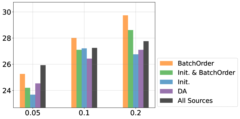
learning rate

Weight Decay
test accuracy %   All-K classes (K=10)

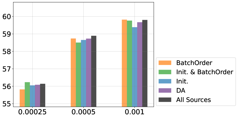
weight decay Top-K classes (K=10)

weight decay Bottom-K classes (K=10)

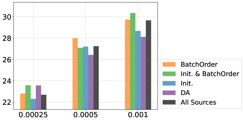
weight decay

Figure 28: Average Eval Accuracy on TinyImageNet as learning rate and weight decay increases. 0.1 is default learning rate, and 0.0005 is default weight decay.

In Appendix B. of (Fort et al., 2019), the authors note that at higher learning rates, mini-batch shuffling adds more randomness than model initialization due to gradient noise. Since our experiments for CIFAR-100 and TinyImageNet use higher learning rates, this is in line with the observations from (Fort et al., 2019). Additionally, we also perform an ablation on learning rates fig. 28 in Appendix H where one can clearly see the impact of different hyperparameters onto the final conclusions. There are also several works to-date that have considered how stochasticity can impact top-line metrics (Nagarajan et al., 2018). Most relevant to our work is (Qian et al., 2021; Zhuang et al., 2022; Madhyastha & Jain, 2019; Summers & Dinneen, 2021) that evaluates how stochasticity in training impacts fairness in DNN Systems. However, all the existing works have restricted their treatment to a single model setting, and do not evaluate the impact of ensembling.

5 Conclusion and Future Work

In this work, we establish that while ensembling DNNs is often seen as a method of improving average performance, it can also provide significant fairness gains–even when the apparent diversity of the individual models is limited, e.g., only varying through the batch ordering or parameter initialization. Our method does not need fine-grained label information about the root cause of unfair predictions. Regardless of the actual attribute that may be the source or recipient of unfair performances, FAIR-ensembles will improve the bottom group performance. This suggests that homogeneous ensembles are a powerful tool to improve fairness outcomes in sensitive domains where human welfare is at risk, as long as the number of employed models is pushed further even after the average performance plateaus (recall section 3). Our observations led us to precisely understand the cause for the fairness emergence. In short, by controlling the different sources of randomness, we were not only able to measure the impact of each source onto the final ensemble diversity, but we were also able to pinpoint initialization and batch ordering as the main source of diversity. We hope that our observations will open the door to address fairness in homogeneous ensemble through a principled and carefully designed control of the sources of stochasticity in DNN training.

Limitations: Validity on non-DNN models/non-image datasets. While our study focuses on image datasets and DNNs, we found that the fairness benefits of homogeneous ensembles extend beyond such settings. For example, we have conducted additional experiments on the Adult Census Income dataset(Becker & Kohavi, 1996) using both a 3-layer multi-layer perceptron (MLP) model and a Decision Trees model. In the MLP setting, we used both race and sex as sensitive attributes. We trained on the remaining 12 features to predict income level $>$$50k. Using the same ablations as our DNN experiments we report in table 2: homogeneous ensembling improves the $>$$50k Amer-Indian-Eskimo subgroup prediction performance by $2.53$%. As for the Decision Trees, we limited the max depth to be 10 and used the random state, which affects the random feature permutation, as the source of stochasticity to control. The results, shown in table 3, depict improved fairness for Black and Amer-Indian-Eskimo. The $>$$50k Other races subgroup had an outsized improvement with a $3.84$% increase in accuracy over the base model. This motivates the need to develop novel theories explaining the fairness benefits of homogeneous ensembles, as those benefits are not limited to DNNs or image datasets.

Appendix A Experimental Setup

A.1 Sampling

Given a pool of M models, for each ensemble size S we sample 100 times with replacement. We then average the accuracy across the 100 samples plus one base model that is shared across all variants. The result at each S is reported until an ensemble of M models is reached.

A.2 CIFAR-100 Training

We use the following architectures: ResNet9 (He et al., 2016a), VGG16 (Simonyan & Zisserman, 2014) and MLP-Mixer (Tolstikhin et al., 2021). We train them as follows:

ResNet-9 We train the model for 24 steps using Stochastic Gradient Descent (SGD). We implemented standard data augmentation by applying Random Horizontal Flip, Random Translate, and Cutout. We use a Slanted Triangular Learning Rate (SLTR) (Howard & Ruder, 2018). The top-1 test set accuracy is 72.24%

ResNet18/34/50 For these 3 ResNet architectures, we train the model for 50 epochs using Stochastic Gradient Descent (SGD), batch size of 512, momentum=0.9, and weight decay=0.0005. We implemented standard data augmentation by applying Random Horizontal Flip, Random Crop, Random Affine, and Cutout. We use a combination of warmup for the first 5 epoch and cosine annealing for scheduler. The top-1 test set accuracy for ResNet-18 is 73.56%, ResNet-34 is 74.24%, and ResNet-50 is 74.89%

VGG16 We train the model for 130 epochs using Stochastic Gradient Descent (SGD). We implemented standard data augmentation by applying Random Horizontal Flip, Random Crop, and Random Rotation. We use a combination of warmup for 1 epoch and a multi-step scheduler with milestones at steps 60 and 120. The top-1 test set accuracy is 71.23%

MLP-Mixer We train the model for 300 steps using Adaptive Moment Estimation (Adam) (Kingma & Ba, 2014). We implemented standard data augmentation by applying Random Crop, AutoAugment (CIFAR10 Policy) (Cubuk et al., 2018), and CutMix (Yun et al., 2019). We use a combination of warmup for the first 5 epoch and cosine annealing for scheduler. The top-1 test set accuracy is 60.28%

A.3 TinyImageNet Training

We use the following architectures: ResNets (He et al., 2016a), VGG-16 (Simonyan & Zisserman, 2014) and ViT (Dosovitskiy et al., 2020). We train them as follows:

ResNets We train 3 different architectures from the ResNet family (ResNet18, 34, 50) for 100 steps using Stochastic Gradient Descent (SGD). We implemented standard data augmentation by applying Random Resized Crop and Random Horizontal Flip. We use a Slanted Triangular Learning Rate (SLTR) (Howard & Ruder, 2018). The top-1 test set accuracy for ResNet-18 is 49.27%, ResNet-34 is 52.18%, and ResNet-50 is 54.99%

VGG16 We train the model for 100 steps using Stochastic Gradient Descent (SGD). We implemented standard data augmentation by applying Random Resized Crop and Random Horizontal Flip. We use a Slanted Triangular Learning Rate (SLTR) (Howard & Ruder, 2018). The top-1 test set accuracy is 60.37%

ViT We train the model for 100 steps using Adaptive Moment Estimation with decoupled weight decay (AdamW) (Loshchilov & Hutter, 2017). We implemented standard data augmentation by applying Random Horizontal Flip, Random Resized Crop, AutoAugment (Cubuk et al., 2018), Random Erasing (Zhong et al., 2020), Cutmix (Yun et al., 2019), and Mixup(Zhang et al., 2017). We use a combination of warmup for the first 10 epoch and cosine annealing (Loshchilov & Hutter, 2016) for scheduler. The top-1 test set accuracy is 51.21%

Appendix B FAIR-Ensemble: When Homogeneous Ensemble Disproportionately Benefit Minority Groups

B.1 Experimental Setup

B.2 Balanced Dataset Sub-Groups

test accuracy %

B.3 CIFAR-100

ResNet9

ensemble/base

Init

BatchOrder

DA

Init & BatchOrder

ResNet18

ensemble/base

Init

BatchOrder

DA

Init & BatchOrder

ResNet34

ensemble/base

Init

BatchOrder

DA

Init & BatchOrder

ResNet50

ensemble/base

Init

BatchOrder

DA

Init & BatchOrder

VGG16

ensemble/base

Init

B.4 TinyImageNet

ResNet9

ensemble/base

Init

BatchOrder

DA

Init & BatchOrder

ResNet18

ensemble/base

Init

BatchOrder

DA

Init & BatchOrder

ResNet34

ensemble/base

Init

BatchOrder

DA

Init & BatchOrder

ResNet50

ensemble/base

Init

BatchOrder

DA

Init & BatchOrder

VGG16

ensemble/base

Init

K=5

Appendix C Controlling for the Sources of Stochasticity in Homogeneous Ensembles

C.1 CIFAR100 Accuracy % difference for ResNet 18, 34, 50

ResNet family on CIFAR100
% accuracy diff.  

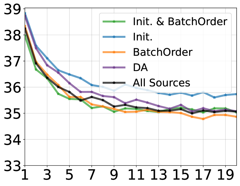
models in ensemble

(a) ResNet18, 20 models

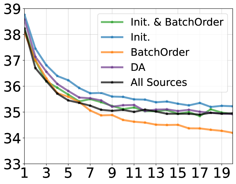
models in ensemble

(b) ResNet34, 20 models

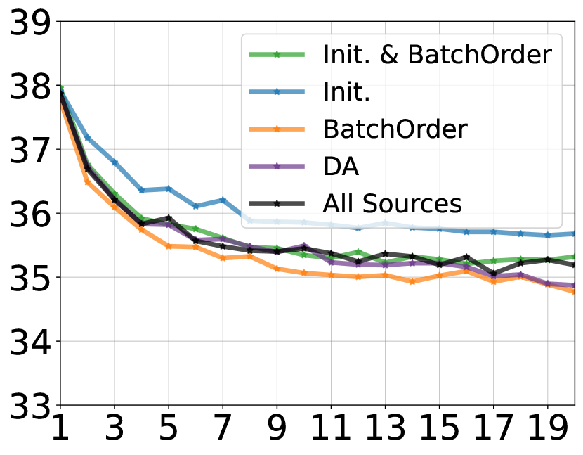
models in ensemble

(c) ResNet50, 20 models

Figure 15: Accuracy % difference between top and bottom 10 classes, for ResNet18, 34, and 50 for CIFAR100.

C.2 CIFAR100 and TinyImageNet Results

CIFAR100 Top-K
test accuracy %   ResNet9
VGG16
MLP-Mixer

CIFAR100 Bottom-K
test accuracy %   ResNet9
VGG16
MLP-Mixer

TinyImageNet Top-K
test accuracy %   ResNet50
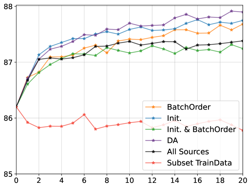
VGG16
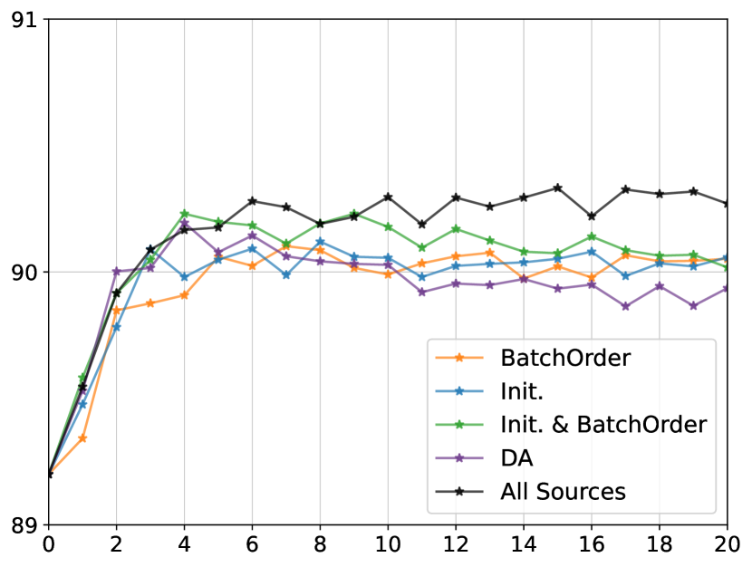
ViT

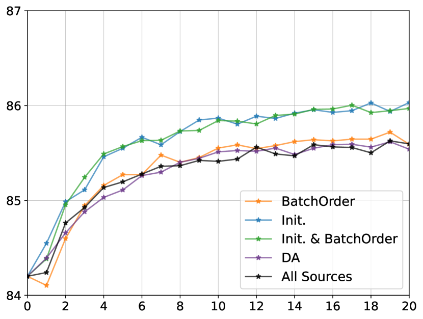
TinyImageNet Bottom-K
test accuracy %   ResNet50

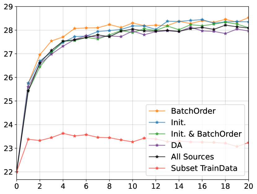
models in ensemble VGG16

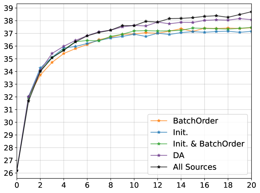
models in ensemble ViT

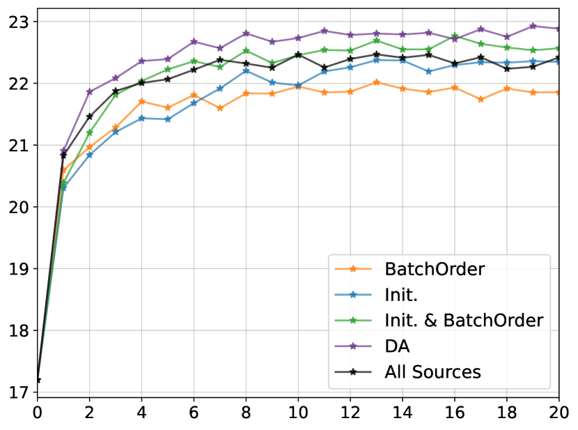
models in ensemble

Figure 17: Average Test Accuracy on CIFAR100 and TinyImageNet for Top-K and Bottom-K ($K=10$) Performing Classes

C.3 Dominant sources of stochasticity

CIFAR100 Accuracy % difference
% accuracy diff.   ResNet9

models in ensemble VGG16

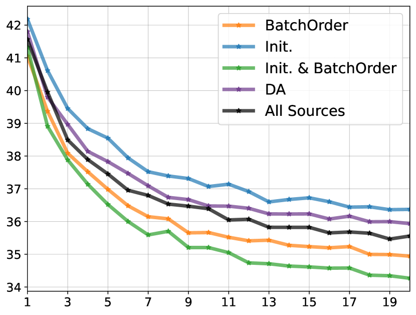
models in ensemble MLP-Mixer

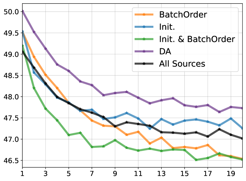
models in ensemble

TinyImageNet Accuracy % difference
% accuracy diff.   ResNet9

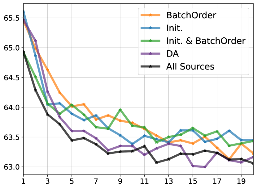
models in ensemble VGG16

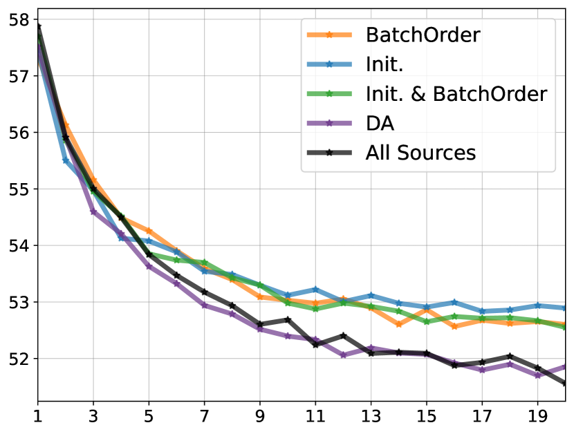
models in ensemble ViT

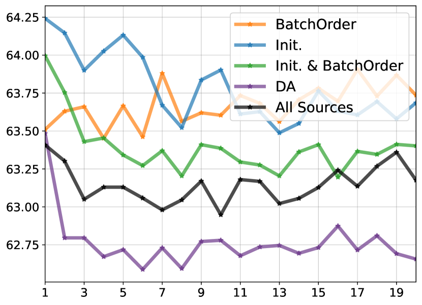
models in ensemble

Figure 18: Accuracy % difference between top and bottom 10 classes for ResNet-9, VGG16, and MLPMixer trained on CIFAR100 and TinyImageNet

Appendix D Results and Discussion

D.1 Comparison between ResNet Architectures

Top-K
test accuracy %   ResNet9

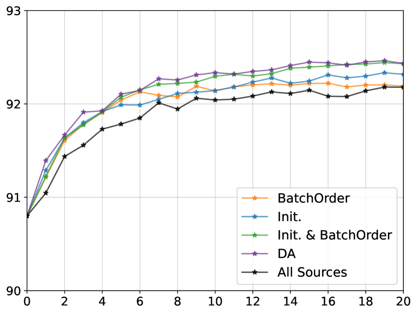
models in ensemble ResNet18

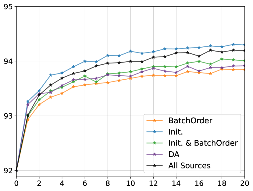
models in ensemble ResNet34

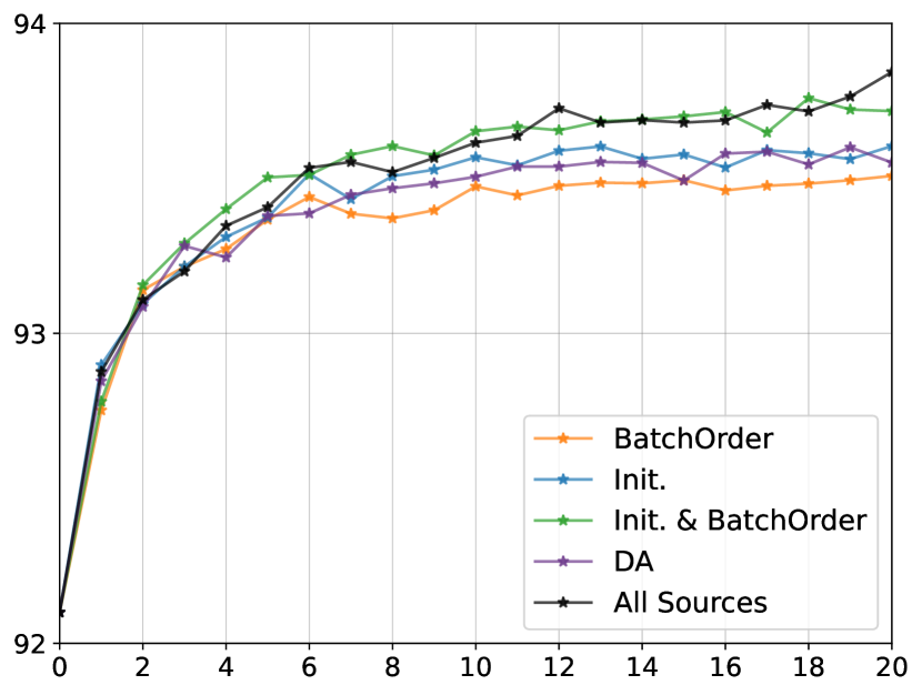
models in ensemble ResNet50

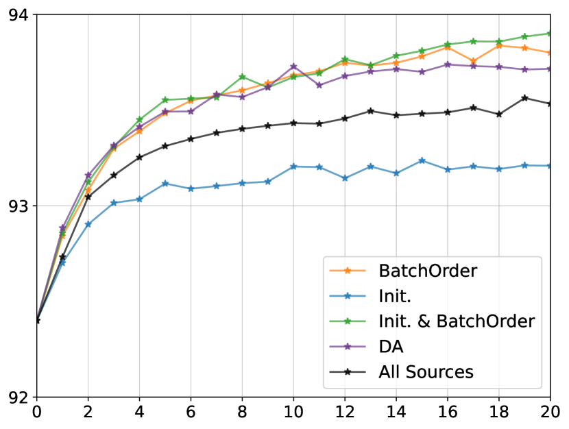
models in ensemble

Bottom-K
test accuracy %   ResNet9

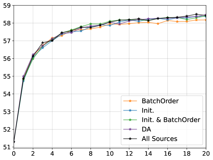
models in ensemble ResNet18

models in ensemble ResNet34

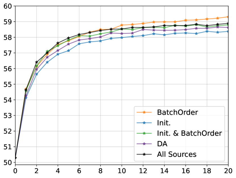
models in ensemble ResNet50

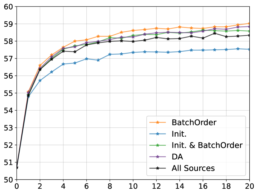
models in ensemble

Figure 19: Average Test Accuracy on CIFAR100 for Top-K and Bottom-K classes across different sizes of ResNets.

D.2 Benefits of even larger homogeneous ensembles

test accuracy %

D.3 CIFAR-100

Resent9 20 model ensemble

ensemble/base

Init

BatchOrder

D.4 TinyImageNet

ResNet50 20 model ensemble

ensemble/base

Init

BatchOrder

DA

Init & BatchOrder

All Sources

ResNet50 30 model ensemble

ensemble/base

Init

BatchOrder

DA

Init & BatchOrder

All Sources

ResNet50 50 model ensemble

ensemble/base

Init

BatchOrder

DA

Init & BatchOrder

All Sources

ResNet34 20 model ensemble

ensemble/base

Init

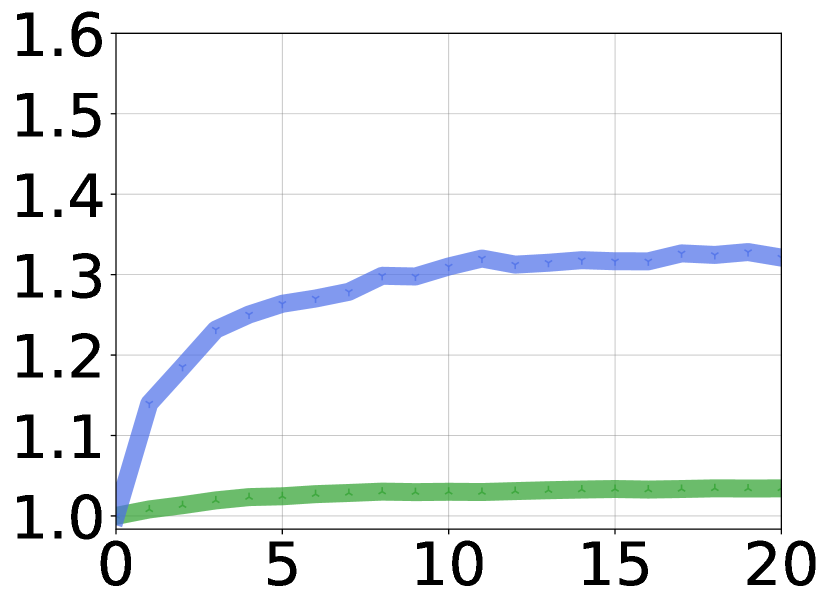
BatchOrder

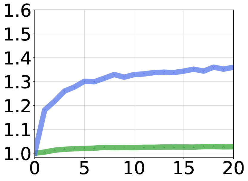
DA

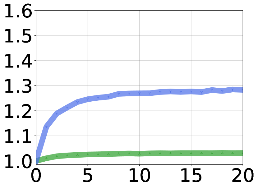
Init & BatchOrder

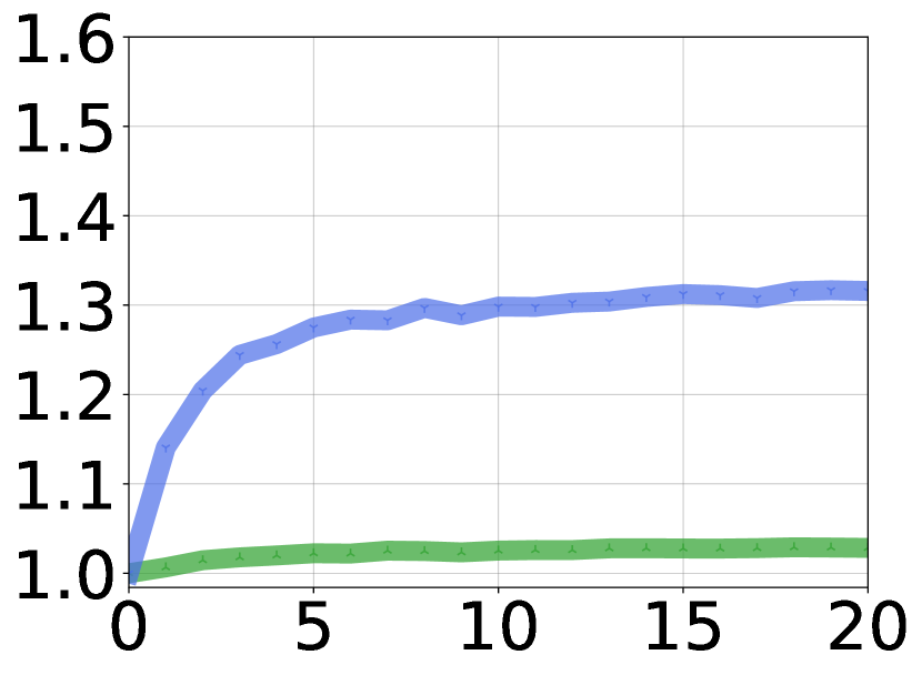
All Sources

VGG16 20 model ensemble

ensemble/base

Init

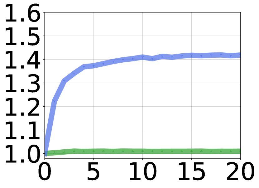
BatchOrder

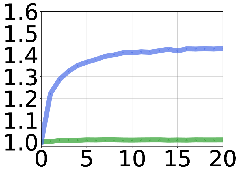
DA

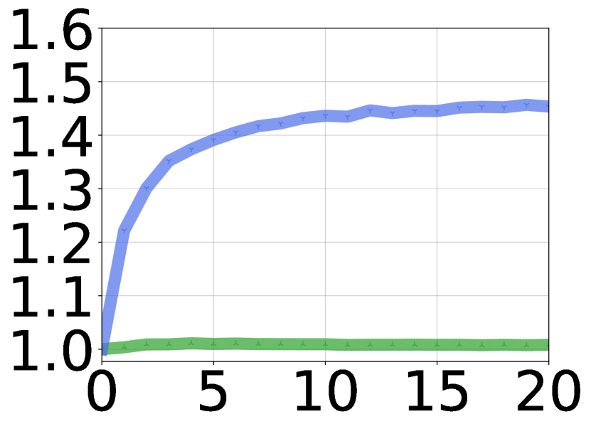
Init & BatchOrder

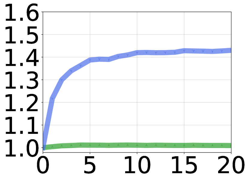
All Sources

ViT 20 model ensemble

ensemble/base

Init

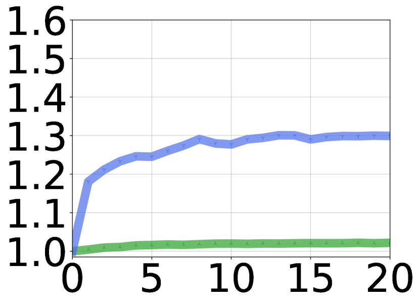
   models in ensemble

BatchOrder

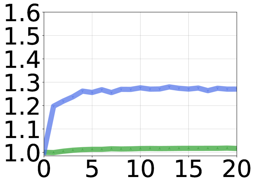
   models in ensemble

DA

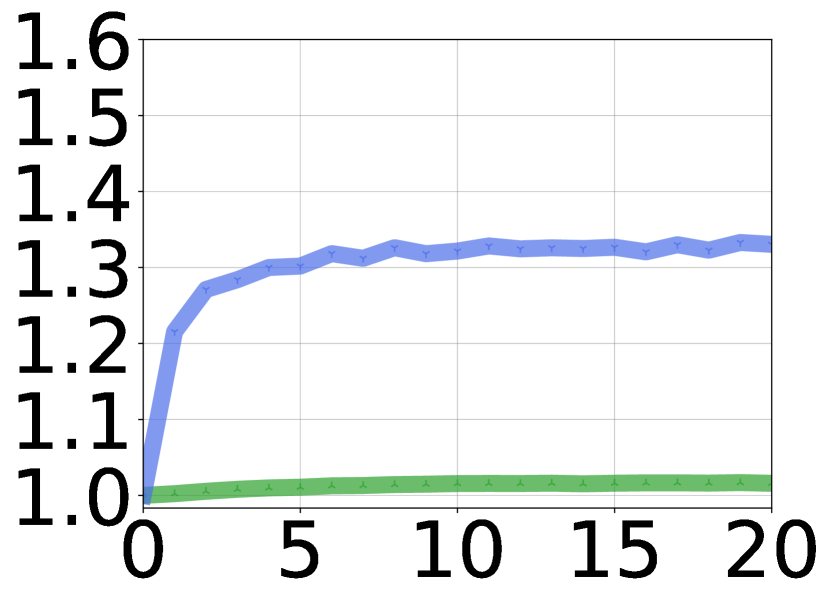
   models in ensemble

Init & BatchOrder

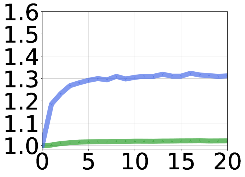
   models in ensemble

All Sources

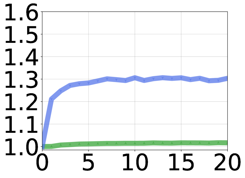
   models in ensemble

Figure 23: Ratio of Top & Bottom K ensemble accuracy for different model architectures and ensemble sizes on TinyImageNet

Appendix E FAIR Ensemble: Improved Robustness

models in ensemble

(a) ResNet-9

Appendix F Difference in Churn Between Models Explains Ensemble Fairness

Churn(%) vs Relative Test Accuracy Improvement(%)
CIFAR TinyImageNet

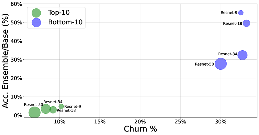
Figure 26: Correlation between Model Disagreement and Ensemble Performance

Appendix G Can Different Sources of Stochasticity Improve Homogeneous Deep Ensemble Fairness?

G.1 Contribution of stochasticity in ensembles

Batch Sizes
test accuracy %   All-K classes (K=10)

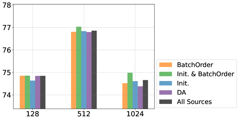
batch size Top-K classes (K=10)

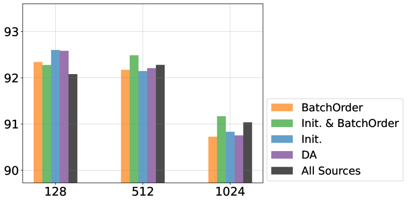
batch size Bottom-K classes (K=10)

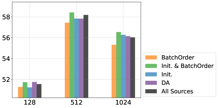
batch size

ResNet Architectures
test accuracy %   All-K classes (K=10)

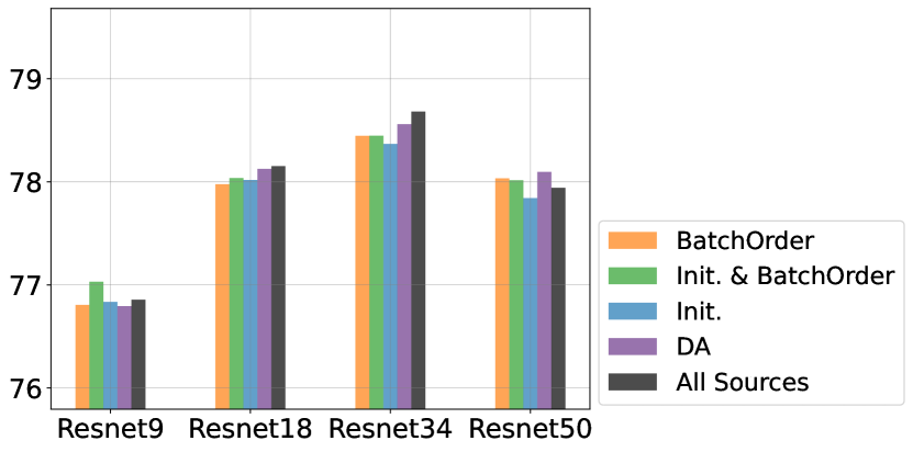
network architecture Top-K classes (K=10)

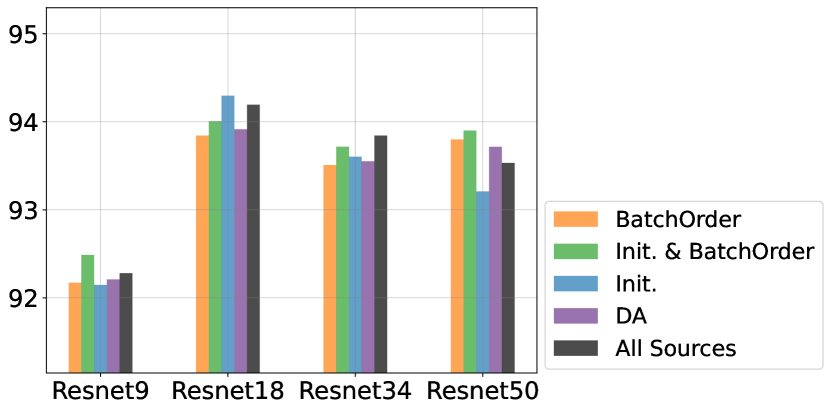
network architecture Bottom-K classes (K=10)

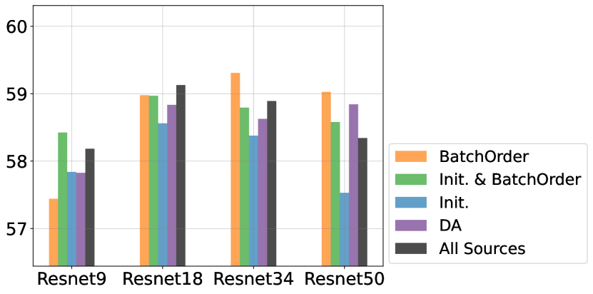
network architecture

Figure 27: Average Test Accuracy on CIFAR100 as batch and architecture size increases. Batch 512 is default.

Learning Rate
test accuracy %   All-K classes (K=10)

learning rate Top-K classes (K=10)

learning rate Bottom-K classes (K=10)

Appendix H Homogeneous ensembles in non-DNN models/non-image datasets

Table 2: MLP ensemble performance over Adult Census Income subgroups with sensitive attributes

		10-model ensemble
	Base Model	BatchOrder	Initialization	Init & BatchOrder	All Sources
$>$$50k	79.93	79.87 $\pm$ 0.03	79.75 $\pm$ 0.28	79.57 $\pm$ 0.38	79.68 $\pm$ 0.21
$>$$50k Male	25.98	26.75 $\pm$ 0.19	26.1 $\pm$ 0.49	27.17 $\pm$ 0.83	26.96 $\pm$ 0.51
$>$$50k Female	27.97	28.63 $\pm$ 0.21	28.23 $\pm$ 0.41	28.93 $\pm$ 0.81	28.76 $\pm$ 0.4
$>$$50k White	26.48	27.22 $\pm$ 0.17	26.64 $\pm$ 0.47	27.61 $\pm$ 0.81	27.4 $\pm$ 0.48
$>$$50k Nonwhite	24.44	25.2 $\pm$ 0.45	24.25 $\pm$ 0.6	25.83 $\pm$ 0.88	25.62 $\pm$ 0.62
$>$$50k Black	24.02	25.29 $\pm$ 0.67	23.92 $\pm$ 0.74	25.89 $\pm$ 0.66	25.73 $\pm$ 0.57
$>$$50k Asian-Pac-Islander	23.31	23.64 $\pm$ 0.39	22.82 $\pm$ 0.52	24.14 $\pm$ 0.96	23.98 $\pm$ 0.7
$>$$50k Amer-Indian-Eskimo	26.32	26.32 $\pm$ 0	27.79 $\pm$ 3.5	28.85 $\pm$ 4.73	27.74 $\pm$ 3.14
$>$$50k Other	32	32 $\pm$ 0	31.44 $\pm$ 1.39	32.12 $\pm$ 0.68	32.04 $\pm$ 0.4

Table 3: Decision Trees ensemble performance over Adult Census Income subgroups with sensitive attributes

	Base Model	10-Model Ensemble
$>$$50k	85.85	85.91 $\pm$ 0.02
$>$$50k Male	60.26	60.35 $\pm$ 0.04
$>$$50k Female	55.59	56.04 $\pm$ 0.09
$>$$50k White	59.89	59.99 $\pm$ 0.05
$>$$50k Nonwhite	56.18	56.73 $\pm$ 0.05
$>$$50k Black	52.51	52.51 $\pm$ 0
$>$$50k Asian-Pac-Islander	61.65	62.41 $\pm$ 0
$>$$50k Amer-Indian-Eskimo	63.16	63.16 $\pm$ 0
$>$$50k Other	48	51.84 $\pm$ 0.78

Appendix I Top and Bottom Classes for CIFAR100 and TinyImageNet

I.1 CIFAR100

Table 4: Top-10 and Bottom-10 class names for CIFAR100. The classes are from the averaged test accuracies from the 20-model ensembles.

ResNet9	ResNet18	ResNet34	ResNet50	VGG16	MLP-Mixer
Top-10
wardrobe	skunk	skunk	orange	road	wardrobe
motorcycle	orange	road	wardrobe	wardrobe	motorcycle
orange	motorcycle	orange	motorcycle	sunflower	orange
skunk	road	sunflower	skunk	motorcycle	sunflower
road	wardrobe	motorcycle	road	skyscraper	road
chimpanzee	palm_tree	wardrobe	sunflower	skunk	skyscraper
sunflower	chimpanzee	palm_tree	chimpanzee	palm_tree	keyboard
orchid	sunflower	pickup_truck	palm_tree	orange	palm_tree
mountain	tractor	aquarium_fish	aquarium_fish	chair	plain
apple	skyscraper	skyscraper	lawn_mower	chimpanzee	skunk
Bottom-10
man	mouse	shark	girl	possum	mouse
shark	bear	possum	lizard	crocodile	bowl
lizard	shark	crocodile	possum	girl	woman
bowl	girl	lizard	maple_tree	shark	girl
possum	lizard	girl	bear	bear	squirrel
shrew	man	man	otter	lizard	possum
seal	otter	bowl	bowl	seal	lizard
girl	seal	otter	man	boy	boy
otter	bowl	seal	boy	otter	otter
boy	boy	boy	seal	man	seal

I.2 TinyImageNet

Table 5: Top-10 and Bottom-10 wnid names for TinyImageNet. The names are from the averaged test accuracies from the 20-model ensembles.

ResNet9	ResNet18	ResNet34	ResNet50	VGG16	ViT
Top-10
n02791270	n02791270	n02791270	n02791270	n02791270	n07875152
n02509815	n02509815	n02509815	n02509815	n03042490	n03814639
n03976657	n02906734	n02906734	n02906734	n02509815	n03983396
n02124075	n03042490	n03814639	n03042490	n03814639	n03042490
n03814639	n03814639	n01950731	n01950731	n02906734	n02823428
n03089624	n03976657	n03599486	n04067472	n01950731	n03599486
n03983396	n01950731	n03042490	n03599486	n04398044	n02509815
n02002724	n04560804	n03976657	n03976657	n02124075	n02791270
n03126707	n03599486	n04067472	n07579787	n03089624	n03126707
n03447447	n02002724	n03126707	n03126707	n04067472	n02906734
Bottom-10
n02437312	n04532670	n03160309	n03544143	n02085620	n02927161
n04070727	n03544143	n01945685	n03617480	n04417672	n03544143
n02268443	n04486054	n04417672	n04070727	n02268443	n04070727
n01945685	n02268443	n04532670	n03804744	n04486054	n01641577
n02226429	n03160309	n03617480	n03160309	n01945685	n02094433
n02233338	n03617480	n01855672	n01945685	n02094433	n02480495
n02480495	n01855672	n03804744	n02268443	n04070727	n02410509
n02410509	n02480495	n02480495	n02480495	n02480495	n04532670
n03617480	n02123394	n02123394	n02123394	n02410509	n02950826
n02123394	n02410509	n02410509	n02410509	n02123394	n02123394

References

- Arulkumaran et al. (2017) Kai Arulkumaran, Marc Peter Deisenroth, Miles Brundage, and Anil Anthony Bharath. A brief survey of deep reinforcement learning. arXiv preprint arXiv:1708.05866, 2017.
- Balestriero et al. (2022) Randall Balestriero, Leon Bottou, and Yann LeCun. The effects of regularization and data augmentation are class dependent. Advances in Neural Information Processing Systems, 35:37878–37891, 2022.
- Barocas et al. (2019) Solon Barocas, Moritz Hardt, and Arvind Narayanan. Fairness and Machine Learning: Limitations and Opportunities. fairmlbook.org, 2019. http://www.fairmlbook.org.
- Basta et al. (2019) Christine Basta, Marta R. Costa-jussà, and Noe Casas. Evaluating the underlying gender bias in contextualized word embeddings. In Proceedings of the First Workshop on Gender Bias in Natural Language Processing, pp. 33–39, Florence, Italy, August 2019. Association for Computational Linguistics. 10.18653/v1/W19-3805. URL https://aclanthology.org/W19-3805.
- Becker & Kohavi (1996) Barry Becker and Ronny Kohavi. Adult. UCI Machine Learning Repository, 1996. DOI: https://doi.org/10.24432/C5XW20.
- Bhaskaruni et al. (2019) Dheeraj Bhaskaruni, Hui Hu, and Chao Lan. Improving prediction fairness via model ensemble. In 2019 IEEE 31st International Conference on Tools with Artificial Intelligence (ICTAI), pp. 1810–1814, 2019. 10.1109/ICTAI.2019.00273.
- Bolukbasi et al. (2016) Tolga Bolukbasi, Kai-Wei Chang, James Y Zou, Venkatesh Saligrama, and Adam T Kalai. Man is to computer programmer as woman is to homemaker? debiasing word embeddings. Advances in neural information processing systems, 29, 2016.
- Breiman (2001) Leo Breiman. Random forests. Machine learning, 45(1):5–32, 2001.
- Buolamwini & Gebru (2018) Joy Buolamwini and Timnit Gebru. Gender shades: Intersectional accuracy disparities in commercial gender classification. In Conference on fairness, accountability and transparency, pp. 77–91, 2018.
- Chatterjee (2020) Satrajit Chatterjee. Coherent gradients: An approach to understanding generalization in gradient descent-based optimization. arXiv preprint arXiv:2002.10657, 2020.
- Chen et al. (2020) Zhe Chen, Yuyan Wang, Dong Lin, Derek Zhiyuan Cheng, Lichan Hong, Ed H. Chi, and Claire Cui. Beyond point estimate: Inferring ensemble prediction variation from neuron activation strength in recommender systems, 2020.
- Chen et al. (2022) Zhenpeng Chen, Jie M Zhang, Federica Sarro, and Mark Harman. Maat: a novel ensemble approach to addressing fairness and performance bugs for machine learning software. In Proceedings of the 30th ACM Joint European Software Engineering Conference and Symposium on the Foundations of Software Engineering, pp. 1122–1134, 2022.
- Cooper et al. (2023) A. Feder Cooper, Katherine Lee, Madiha Choksi, Solon Barocas, Christopher De Sa, James Grimmelmann, Jon Kleinberg, Siddhartha Sen, and Baobao Zhang. Arbitrariness and prediction: The confounding role of variance in fair classification, 2023.
- Cubuk et al. (2018) Ekin D Cubuk, Barret Zoph, Dandelion Mane, Vijay Vasudevan, and Quoc V Le. Autoaugment: Learning augmentation policies from data. arXiv preprint arXiv:1805.09501, 2018.
- Dietterich (2000) Thomas G Dietterich. Ensemble methods in machine learning. In International workshop on multiple classifier systems, pp. 1–15. Springer, 2000.
- Dosovitskiy et al. (2020) Alexey Dosovitskiy, Lucas Beyer, Alexander Kolesnikov, Dirk Weissenborn, Xiaohua Zhai, Thomas Unterthiner, Mostafa Dehghani, Matthias Minderer, Georg Heigold, Sylvain Gelly, et al. An image is worth 16x16 words: Transformers for image recognition at scale. arXiv preprint arXiv:2010.11929, 2020.
- Feldman & Zhang (2020) Vitaly Feldman and Chiyuan Zhang. What neural networks memorize and why: Discovering the long tail via influence estimation. In H. Larochelle, M. Ranzato, R. Hadsell, M. F. Balcan, and H. Lin (eds.), Advances in Neural Information Processing Systems, volume 33, pp. 2881–2891. Curran Associates, Inc., 2020. URL https://proceedings.neurips.cc/paper/2020/file/1e14bfe2714193e7af5abc64ecbd6b46-Paper.pdf.
- Fort et al. (2019) Stanislav Fort, Huiyi Hu, and Balaji Lakshminarayanan. Deep ensembles: A loss landscape perspective. arXiv preprint arXiv:1912.02757, 2019.
- Freund & Schapire (1995) Yoav Freund and Robert E. Schapire. A decision-theoretic generalization of on-line learning and an application to boosting. In EuroCOLT, 1995.
- Garg et al. (2017) Nikhil Garg, Londa Schiebinger, Dan Jurafsky, and James Zou. Word embeddings quantify 100 years of gender and ethnic stereotypes. Proceedings of the National Academy of Sciences, 115, 11 2017. 10.1073/pnas.1720347115.
- Glorot & Bengio (2010) Xavier Glorot and Yoshua Bengio. Understanding the difficulty of training deep feedforward neural networks. In Yee Whye Teh and Mike Titterington (eds.), Proceedings of the Thirteenth International Conference on Artificial Intelligence and Statistics, volume 9 of Proceedings of Machine Learning Research, pp. 249–256, Chia Laguna Resort, Sardinia, Italy, 13–15 May 2010. PMLR. URL http://proceedings.mlr.press/v9/glorot10a.html.
- Gohar et al. (2023) Usman Gohar, Sumon Biswas, and Hridesh Rajan. Towards understanding fairness and its composition in ensemble machine learning. In 2023 IEEE/ACM 45th International Conference on Software Engineering (ICSE), pp. 1533–1545. IEEE, 2023.
- Grgić-Hlača et al. (2017) Nina Grgić-Hlača, Muhammad Bilal Zafar, Krishna P. Gummadi, and Adrian Weller. On fairness, diversity and randomness in algorithmic decision making, 2017. URL https://arxiv.org/abs/1706.10208.
- Gupta et al. (2022) Neha Gupta, Jamie Smith, Ben Adlam, and Zelda Mariet. Ensembling over classifiers: a bias-variance perspective. arXiv preprint arXiv:2206.10566, 2022.
- Hashimoto et al. (2018) Tatsunori Hashimoto, Megha Srivastava, Hongseok Namkoong, and Percy Liang. Fairness without demographics in repeated loss minimization. In Jennifer Dy and Andreas Krause (eds.), Proceedings of the 35th International Conference on Machine Learning, volume 80 of Proceedings of Machine Learning Research, pp. 1929–1938, Stockholmsmässan, Stockholm Sweden, 10–15 Jul 2018. PMLR. URL http://proceedings.mlr.press/v80/hashimoto18a.html.
- He et al. (2016a) Kaiming He, Xiangyu Zhang, Shaoqing Ren, and Jian Sun. Deep residual learning for image recognition. In CVPR, 2016a.
- He et al. (2016b) Kaiming He, Xiangyu Zhang, Shaoqing Ren, and Jian Sun. Deep residual learning for image recognition. In 2016 IEEE Conference on Computer Vision and Pattern Recognition, CVPR, 2016b.
- Hendrycks & Dietterich (2018) Dan Hendrycks and Thomas G Dietterich. Benchmarking neural network robustness to common corruptions and surface variations. arXiv preprint arXiv:1807.01697, 2018.
- Hernández-García & König (2018) Alex Hernández-García and Peter König. Further advantages of data augmentation on convolutional neural networks. Lecture Notes in Computer Science, pp. 95–103, 2018. ISSN 1611-3349. 10.1007/978-3-030-01418-6_10. URL http://dx.doi.org/10.1007/978-3-030-01418-6_10.
- Hinton et al. (2012) Geoffrey Hinton, Li Deng, Dong Yu, George E Dahl, Abdel-rahman Mohamed, Navdeep Jaitly, Andrew Senior, Vincent Vanhoucke, Patrick Nguyen, Tara N Sainath, et al. Deep neural networks for acoustic modeling in speech recognition: The shared views of four research groups. IEEE Signal processing magazine, 29(6):82–97, 2012.
- Hooker et al. (2019) Sara Hooker, Aaron Courville, Gregory Clark, Yann Dauphin, and Andrea Frome. What Do Compressed Deep Neural Networks Forget? arXiv e-prints, art. arXiv:1911.05248, November 2019.
- Hooker et al. (2019) Sara Hooker, Aaron Courville, Gregory Clark, Yann Dauphin, and Andrea Frome. What do compressed deep neural networks forget? arXiv, 2019.
- Howard & Ruder (2018) Jeremy Howard and Sebastian Ruder. Universal language model fine-tuning for text classification. arXiv preprint arXiv:1801.06146, 2018.
- Jain et al. (2020) Siddhartha Jain, Ge Liu, Jonas Mueller, and David Gifford. Maximizing overall diversity for improved uncertainty estimates in deep ensembles. In Proceedings of the AAAI Conference on Artificial Intelligence, volume 34, pp. 4264–4271, 2020.
- Kenfack et al. (2021) Patrik Joslin Kenfack, Adil Mehmood Khan, SM Ahsan Kazmi, Rasheed Hussain, Alma Oracevic, and Asad Masood Khattak. Impact of model ensemble on the fairness of classifiers in machine learning. In 2021 International conference on applied artificial intelligence (ICAPAI), pp. 1–6. IEEE, 2021.
- Kingma & Ba (2014) Diederik P Kingma and Jimmy Ba. Adam: A method for stochastic optimization. arXiv preprint arXiv:1412.6980, 2014.
- Kleinberg et al. (2016) Jon M. Kleinberg, Sendhil Mullainathan, and Manish Raghavan. Inherent trade-offs in the fair determination of risk scores. CoRR, abs/1609.05807, 2016. URL http://arxiv.org/abs/1609.05807.
- Krizhevsky et al. (2009) Alex Krizhevsky, Geoffrey Hinton, et al. Learning multiple layers of features from tiny images. 2009.
- Kukačka et al. (2017) Jan Kukačka, Vladimir Golkov, and Daniel Cremers. Regularization for deep learning: A taxonomy, 2017.
- Lakshminarayanan et al. (2016) Balaji Lakshminarayanan, Alexander Pritzel, and Charles Blundell. Simple and Scalable Predictive Uncertainty Estimation using Deep Ensembles. arXiv e-prints, art. arXiv:1612.01474, Dec 2016.
- Lee et al. (2015) Stefan Lee, Senthil Purushwalkam, Michael Cogswell, David J. Crandall, and Dhruv Batra. Why M heads are better than one: Training a diverse ensemble of deep networks. CoRR, abs/1511.06314, 2015. URL http://arxiv.org/abs/1511.06314.
- Liu et al. (2015) Ziwei Liu, Ping Luo, Xiaogang Wang, and Xiaoou Tang. Deep learning face attributes in the wild. In Proceedings of International Conference on Computer Vision (ICCV), December 2015.
- Loshchilov & Hutter (2016) Ilya Loshchilov and Frank Hutter. Sgdr: Stochastic gradient descent with warm restarts. arXiv preprint arXiv:1608.03983, 2016.
- Loshchilov & Hutter (2017) Ilya Loshchilov and Frank Hutter. Decoupled weight decay regularization. arXiv preprint arXiv:1711.05101, 2017.
- Madhyastha & Jain (2019) Pranava Madhyastha and Rishabh Jain. On model stability as a function of random seed. arXiv preprint arXiv:1909.10447, 2019.
- Milani Fard et al. (2016) Mahdi Milani Fard, Quentin Cormier, Kevin Canini, and Maya Gupta. Launch and iterate: Reducing prediction churn. In D. Lee, M. Sugiyama, U. Luxburg, I. Guyon, and R. Garnett (eds.), Advances in Neural Information Processing Systems, volume 29. Curran Associates, Inc., 2016. URL https://proceedings.neurips.cc/paper/2016/file/dc5c768b5dc76a084531934b34601977-Paper.pdf.
- Nagarajan et al. (2018) Prabhat Nagarajan, Garrett Warnell, and Peter Stone. The impact of nondeterminism on reproducibility in deep reinforcement learning. In Reproducibility in ML Workshop at the 35th International Conference on Machine Learning, ICML, 2018.
- Ogueji et al. (2022) Kelechi Ogueji, Orevaoghene Ahia, Gbemileke Onilude, Sebastian Gehrmann, Sara Hooker, and Julia Kreutzer. Intriguing properties of compression on multilingual models, 2022. URL https://arxiv.org/abs/2211.02738.
- Opitz & Maclin (1999) D. Opitz and R. Maclin. Popular ensemble methods: An empirical study. Journal of Artificial Intelligence Research, 11:169–198, aug 1999. 10.1613/jair.614. URL https://doi.org/10.1613%2Fjair.614.
- Qian et al. (2021) Shangshu Qian, Viet Hung Pham, Thibaud Lutellier, Zeou Hu, Jungwon Kim, Lin Tan, Yaoliang Yu, Jiahao Chen, and Sameena Shah. Are my deep learning systems fair? an empirical study of fixed-seed training. Advances in Neural Information Processing Systems, 34:30211–30227, 2021.
- Rame et al. (2022) Alexandre Rame, Matthieu Kirchmeyer, Thibaud Rahier, Alain Rakotomamonjy, Patrick Gallinari, and Matthieu Cord. Diverse weight averaging for out-of-distribution generalization. arXiv preprint arXiv:2205.09739, 2022.
- Russakovsky et al. (2015) Olga Russakovsky, Jia Deng, Hao Su, Jonathan Krause, Sanjeev Satheesh, Sean Ma, Zhiheng Huang, Andrej Karpathy, Aditya Khosla, Michael Bernstein, et al. Imagenet large scale visual recognition challenge. In IJCV, 2015.
- Shallue et al. (2019) Christopher J. Shallue, Jaehoon Lee, Joseph Antognini, Jascha Sohl-Dickstein, Roy Frostig, and George E. Dahl. Measuring the effects of data parallelism on neural network training, 2019.
- Shamir & Coviello (2020) Gil I. Shamir and Lorenzo Coviello. Anti-distillation: Improving reproducibility of deep networks. CoRR, abs/2010.09923, 2020. URL https://arxiv.org/abs/2010.09923.
- Shankar et al. (2017) Shreya Shankar, Yoni Halpern, Eric Breck, James Atwood, Jimbo Wilson, and D Sculley. No classification without representation: Assessing geodiversity issues in open data sets for the developing world. arXiv preprint arXiv:1711.08536, 2017.
- Shumailov et al. (2021) Ilia Shumailov, Zakhar Shumaylov, Dmitry Kazhdan, Yiren Zhao, Nicolas Papernot, Murat A. Erdogdu, and Ross Anderson. Manipulating sgd with data ordering attacks, 2021.
- Simonyan & Zisserman (2014) Karen Simonyan and Andrew Zisserman. Very deep convolutional networks for large-scale image recognition. arXiv preprint arXiv:1409.1556, 2014.
- Smith et al. (2018) Samuel L. Smith, Pieter-Jan Kindermans, Chris Ying, and Quoc V. Le. Don’t decay the learning rate, increase the batch size, 2018.
- Snapp & Shamir (2021) Robert R. Snapp and Gil I. Shamir. Synthesizing irreproducibility in deep networks. CoRR, abs/2102.10696, 2021. URL https://arxiv.org/abs/2102.10696.
- Stickland & Murray (2020) Asa Cooper Stickland and Iain Murray. Diverse ensembles improve calibration. CoRR, abs/2007.04206, 2020. URL https://arxiv.org/abs/2007.04206.
- Summers & Dinneen (2021) Cecilia Summers and Michael J Dinneen. Nondeterminism and instability in neural network optimization. In International Conference on Machine Learning, pp. 9913–9922. PMLR, 2021.
- Tolstikhin et al. (2021) Ilya O Tolstikhin, Neil Houlsby, Alexander Kolesnikov, Lucas Beyer, Xiaohua Zhai, Thomas Unterthiner, Jessica Yung, Andreas Steiner, Daniel Keysers, Jakob Uszkoreit, et al. Mlp-mixer: An all-mlp architecture for vision. Advances in Neural Information Processing Systems, 34:24261–24272, 2021.
- Vaswani et al. (2017) Ashish Vaswani, Noam Shazeer, Niki Parmar, Jakob Uszkoreit, Llion Jones, Aidan N. Gomez, Lukasz Kaiser, and Illia Polosukhin. Attention is All you Need. In Advances in Neural Information Processing Systems 30: Annual Conference on Neural Information Processing Systems 2017, 4-9 December 2017, Long Beach, CA, USA, pp. 6000–6010, 2017.
- Veldanda et al. (2022) Akshaj Kumar Veldanda, Ivan Brugere, Jiahao Chen, Sanghamitra Dutta, Alan Mishler, and Siddharth Garg. Fairness via in-processing in the over-parameterized regime: A cautionary tale. arXiv preprint arXiv:2206.14853, 2022.
- Wang et al. (2020) Xiaofang Wang, Dan Kondratyuk, Kris M. Kitani, Yair Movshovitz-Attias, and Elad Eban. Multiple networks are more efficient than one: Fast and accurate models via ensembles and cascades. CoRR, abs/2012.01988, 2020. URL https://arxiv.org/abs/2012.01988.
- Wortsman et al. (2022) Mitchell Wortsman, Gabriel Ilharco, Samir Ya Gadre, Rebecca Roelofs, Raphael Gontijo-Lopes, Ari S Morcos, Hongseok Namkoong, Ali Farhadi, Yair Carmon, Simon Kornblith, et al. Model soups: averaging weights of multiple fine-tuned models improves accuracy without increasing inference time. In International Conference on Machine Learning, pp. 23965–23998. PMLR, 2022.
- Yun et al. (2019) Sangdoo Yun, Dongyoon Han, Seong Joon Oh, Sanghyuk Chun, Junsuk Choe, and Youngjoon Yoo. Cutmix: Regularization strategy to train strong classifiers with localizable features. In Proceedings of the IEEE/CVF international conference on computer vision, pp. 6023–6032, 2019.
- Zafar et al. (2015) Muhammad Bilal Zafar, Isabel Valera, Manuel Gomez Rodriguez, and Krishna P. Gummadi. Fairness constraints: Mechanisms for fair classification, 2015. URL https://arxiv.org/abs/1507.05259.
- Zaidi et al. (2021) Sheheryar Zaidi, Arber Zela, Thomas Elsken, Chris C Holmes, Frank Hutter, and Yee Teh. Neural ensemble search for uncertainty estimation and dataset shift. Advances in Neural Information Processing Systems, 34:7898–7911, 2021.
- Zhang et al. (2017) Hongyi Zhang, Moustapha Cisse, Yann N Dauphin, and David Lopez-Paz. mixup: Beyond empirical risk minimization. arXiv preprint arXiv:1710.09412, 2017.
- Zhao et al. (2017) Jieyu Zhao, Tianlu Wang, Mark Yatskar, Vicente Ordonez, and Kai-Wei Chang. Men also like shopping: Reducing gender bias amplification using corpus-level constraints. In Proceedings of the 2017 Conference on Empirical Methods in Natural Language Processing, September 2017.
- Zhao et al. (2018) Jieyu Zhao, Tianlu Wang, Mark Yatskar, Vicente Ordonez, and Kai-Wei Chang. Gender bias in coreference resolution: Evaluation and debiasing methods. In Proceedings of the 2018 Conference of the North American Chapter of the Association for Computational Linguistics: Human Language Technologies, Volume 2 (Short Papers), pp. 15–20, New Orleans, Louisiana, June 2018. Association for Computational Linguistics. 10.18653/v1/N18-2003. URL https://aclanthology.org/N18-2003.
- Zhong et al. (2020) Zhun Zhong, Liang Zheng, Guoliang Kang, Shaozi Li, and Yi Yang. Random erasing data augmentation. In Proceedings of the AAAI conference on artificial intelligence, volume 34, pp. 13001–13008, 2020.
- Zhuang et al. (2022) Donglin Zhuang, Xingyao Zhang, Shuaiwen Song, and Sara Hooker. Randomness in neural network training: Characterizing the impact of tooling. In D. Marculescu, Y. Chi, and C. Wu (eds.), Proceedings of Machine Learning and Systems, volume 4, pp. 316–336, 2022. URL https://proceedings.mlsys.org/paper/2022/file/757b505cfd34c64c85ca5b5690ee5293-Paper.pdf.