Are More Layers Beneficial to Graph Transformers?

Abstract

Despite that going deep has proven successful in many neural architectures, the existing graph transformers are relatively shallow. In this work, we explore whether more layers are beneficial to graph transformers, and find that current graph transformers suffer from the bottleneck of improving performance by increasing depth. Our further analysis reveals the reason is that deep graph transformers are limited by the vanishing capacity of global attention, restricting the graph transformer from focusing on the critical substructure and obtaining expressive features. To this end, we propose a novel graph transformer model named DeepGraph that explicitly employs substructure tokens in the encoded representation, and applies local attention on related nodes to obtain substructure based attention encoding. Our model enhances the ability of the global attention to focus on substructures and promotes the expressiveness of the representations, addressing the limitation of self-attention as the graph transformer deepens. Experiments show that our method unblocks the depth limitation of graph transformers and results in state-of-the-art performance across various graph benchmarks with deeper models.

1 Introduction

Transformers have recently gained rapid attention in modeling graph-structured data (Zhang et al., 2020; Dwivedi & Bresson, 2020; Maziarka et al., 2020; Ying et al., 2021; Chen et al., 2022). Compared to graph neural networks, graph transformer implies global attention mechanism to enable information passing between all nodes, which is advantageous to learn long-range dependency of the graph stuctures (Alon & Yahav, 2020). In transformer, the graph structure information can be encoded into node feature (Kreuzer et al., 2021) or attentions (Ying et al., 2021) by a variant of methods flexibly with strong expressiveness, avoiding the inherent limitations of encoding paradigms that pass the information along graph edges. Global attention (Bahdanau et al., 2015) also enables explicit focus on essential parts among the nodes to model crucial substructures in the graph.

Graph transformer in current studies is usually shallow, i.e., less than 12 layers. Scaling depth is proven to increase the capacity of neural networks exponentially (Poole et al., 2016), and empirically improve transformer performance in natural language processing (Liu et al., 2020a; Bachlechner et al., 2021) and computer vision (Zhou et al., 2021). Graph neural networks also benefit from more depth when properly designed (Chen et al., 2020a; Liu et al., 2020b; Li et al., 2021). However, it is still not clear whether the capability of graph transformers in graph tasks can be strengthened by increasing model depth. So we conduct experiments and find that current graph transformers encounter the bottleneck of improving performance by increasing depth. The further deepening will hurt performance when model exceeds 12 layers, which seems to be the upper limit of the current graph transformer depth, as Figure 1 (left) shows.

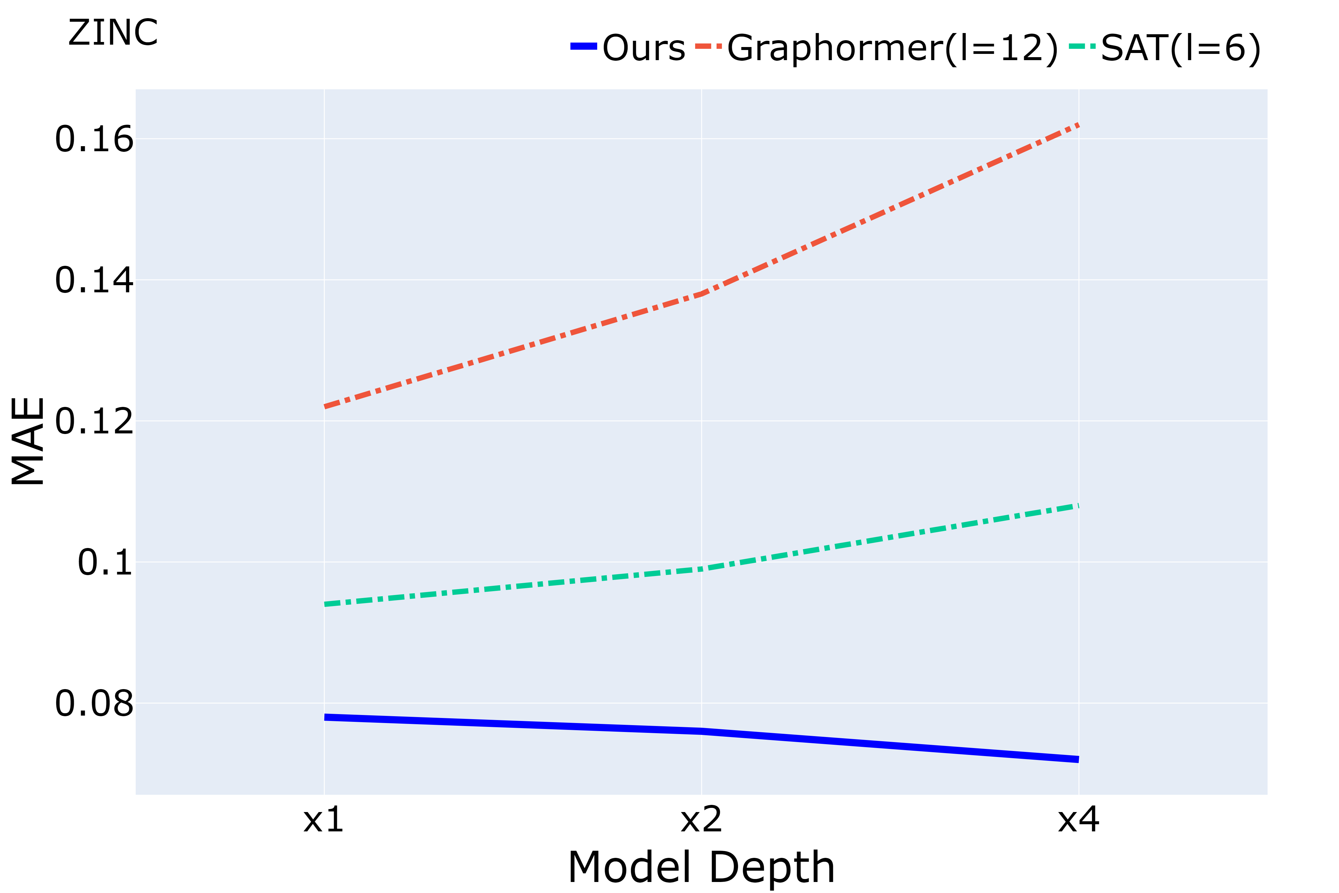
(a)

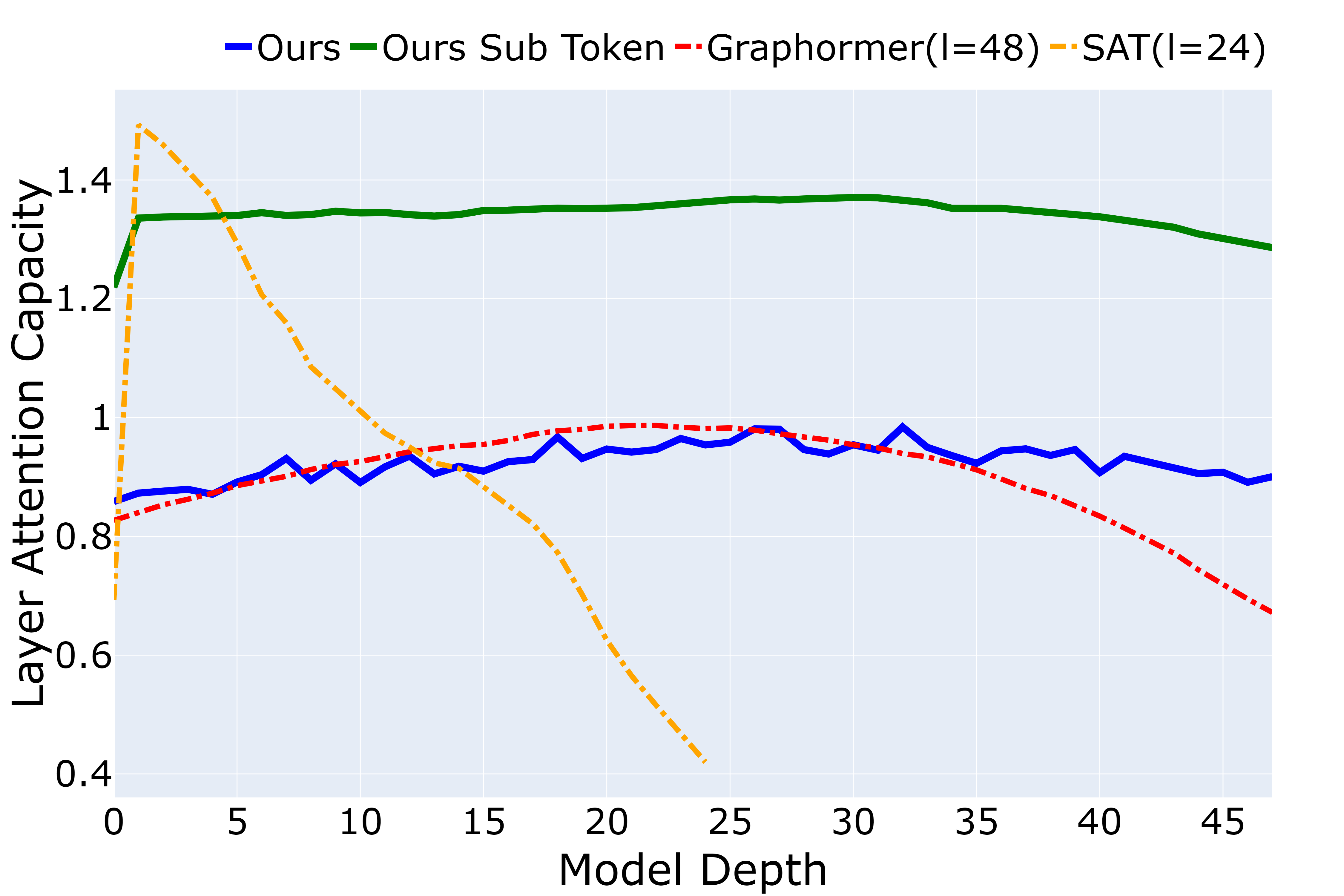
(b)

Figure 1: Left: Performance on ZINC dataset of different graph transformers by varying their depths. Our DeepGraph successfully scales up the depth, while the baselines can not. (Lower is better.) Right: Layer attention capacity to substructures with depth.

In this work, we aim to answer why more self-attention layers become a disadvantage for graph transformers, and how to address these issues with the proper model design. Self-attention (Bahdanau et al., 2015) makes a leap in model capacity by dynamically concentrating on critical parts (Chen et al., 2022), i.e., substructures of a graph, and obtaining particular features. Substructures are the basic intrinsic features of graph data widely used in data analysis (Yu et al., 2020) and machine learning (Shervashidze et al., 2009), as well as graph model interpretability (Miao et al., 2022). Although the self-attention module appears to be very beneficial for automatically learning important substructure features in the graph, our analysis indicates that this ability vanishes as depth grows, restricting the deeper graph transformer from learning useful structure features. Specifically, we focus on the influence of attention on different substructures, which we found to decrease after each self-attention layer. In consequence, it is difficult for deep models to autonomously learn effective attention patterns of substructures and obtain expressive graph substructure features.

We further propose a graph transformer model named DeepGraph with a simple but effective method to enhance substructure encoding ability of deeper graph transformer. The proposed model explicitly introduces local attention mechanism on substructures by employing additional substructure tokens in the model representation and applying local attention to nodes related to those substructures. Our method not only introduces the substructure based attention to encourage the model to focus on substructure feature, but also enlarges the attention capacity theoretically and empirically, which improves the expressiveness of representations learned on substructures.

In summary, our contributions are as follows:

• We present the bottleneck of graph transformers’ performance when depth increases, illustrating the depth limitation of current graph transformers. We study the bottleneck from the perspective of attention capacity decay with layers theoretically and empirically, and demonstrate the difficulty for deep models to learn effective attention patterns of substructures and obtain informative graph substructure features.

• According to the above finding, we propose a simple yet effective local attention mechanism based on substructure tokens, promoting focus on local substructure features of deeper graph transformer and improving the expressiveness of learned representations.

• Experiments show that our method unblocks the depth limitation of graph transformer and achieves state-of-the-art results on standard graph benchmarks with deeper models.

2 Related Work

Graph transformers Transformer with the self-attention has been the mainstream method in nature language processing (Vaswani et al., 2017; Devlin et al., 2019; Liu et al., 2019), and is also proven competitive for image in computer vision (Dosovitskiy et al., 2020). Pure transformers lack relation information between tokens and need position encoding for structure information. Recent works apply transformers in graph tasks by designing a variety of structure encoding techniques. Some works embed structure information into graph nodes by methods including Laplacian vector, random walk, or other feature (Zhang et al., 2020; Dwivedi & Bresson, 2020; Kreuzer et al., 2021; Kim et al., 2022; Wu et al., 2021). Some other works introduce structure information into attention by graph distance, path embedding or feature encoded by GNN (Park et al., 2022; Maziarka et al., 2020; Ying et al., 2021; Chen et al., 2022; Mialon et al., 2021; Choromanski et al., 2022). Other works use transformer as a module of the whole model (Bastos et al., 2022; Guo et al., 2022).

Deep neural networks There are many works focus on solving obstacles and release potential of deep neural networks in feed-forward network (FNN) (Telgarsky, 2016; Yarotsky, 2017) and convolutional neural network (CNN) (He et al., 2016a; Simonyan & Zisserman, 2014; Xiao et al., 2018; He et al., 2016b). For graph neural networks, early studies reveal severe performance degradation when stacking many layers (Li et al., 2019; Xu et al., 2018b; Li et al., 2018), caused by problems including over-smoothing and gradient vanishing (Oono & Suzuki, 2019; Zhao & Akoglu, 2019; Rong et al., 2019; Nt & Maehara, 2019). Recent works alleviate these problems by residual connection, dropout, and other methods (Chen et al., 2020a; Li et al., 2020; 2021), and deepen GNN into hundreds and even thousands of layers with better performance. Deep transformer is also proved powerful in nature language processing (Wang et al., 2022) and computational vision (Zhou et al., 2021), while better initialization (Zhang et al., 2019) or architecture (Wang et al., 2019; Liu et al., 2020a; Bachlechner et al., 2021) are proposed to solve optimization instability and over-smoothing (Shi et al., 2021; Wang et al., 2021; Dong et al., 2021).

Graph substructure Substructure is one of the basic intrinsic features of graph data, which is widely used in both graph data analysis (Shervashidze et al., 2009; Yanardag & Vishwanathan, 2015; Rossi et al., 2020) and deep graph neural models (Chen et al., 2020b; Bouritsas et al., 2022; Bodnar et al., 2021; Zhang & Li, 2021; Zhao et al., 2021). In application, substructure related methods are widely used in various domain including computational chemistry (Murray & Rees, 2009; Jin et al., 2018; 2019; Duvenaud et al., 2015; Yu et al., 2020), computational biology (Koyutürk et al., 2004) and social network (Jiang et al., 2010). Certain substructures can also be the pivotal feature for graph property prediction, which is a fundamental hypothesis in graph model interpretability studies (Ying et al., 2019; Miao et al., 2022), helping to understand how a graph model makes decisions.

3 Preliminary

3.1 Graph and Substructure

We denote graph data as $\{G_{i},y_{i}\}$, where a graph $G=(N,R,x,r)$ includes nodes $N=\{1\dots|G|\}$ and corresponding edges $R\subset N\times N$, while $x$ and $r$ are node features and edge features. Label $y$ can be graph-wise or node-wise, depending on the task definition. Given graph $G$, a substructure is defined as $G^{S}=\{N^{S},R^{S},x^{S},r^{S}\}$, where $N^{S}\subset N,R^{S}=(N^{S}\times N^{S})\cap R$, i.e. nodes of $G^{S}$ form a subset of the graph $G$ and edges are all the existing edges in $G$ between nodes subset, which is also known as induced subgraph. Because attention is only applied to graph nodes, attention to arbitrary subgraphs is not well-defined. Therefore, we only consider induced subgraphs in this work.

3.2 Transformer

The core module of the transformer is self-attention. Let $H_{l}=\left[h_{1},\cdots,h_{n}\right]^{\top}\in\mathbb{R}^{n\times d_{h}}$ be the hidden representation in layer $l$, where $n$ is the number of token, and $d_{h}$ is the dimension of hidden embedding of each token. The self-attention mapping $\hat{\operatorname{Attn}}$ with parameter $W^{V},W^{Q},W^{K}\in\mathbb{R}^{d_{h}\times d_{k}}$ and $W^{O}\in\mathbb{R}^{d_{k}\times d_{h}}$ is

$$\hat{A}=\frac{(H_{l}W^{Q})(H_{l}W^{K})^{\top}}{\sqrt{d_{k}}},\quad A=\operatorname{softmax}(\hat{A}),\quad$$ (1)

$$\hat{\operatorname{Attn}}(H_{l})=AH_{l}W^{V}W^{O}=AH_{l}W^{VO},$$

where $W^{VO}\triangleq W^{V}W^{O}$. In practice, a complete transformer layer also contains a two-layer fully-connected network $\operatorname{FFN}$, and layer normalization with residual connection $\operatorname{LN}$ is also applied to both self-attention module and fully-connected network:

$${H_{l+1}} =\operatorname{FFN}(\operatorname{Attn}(H_{l})),$$ (2)

where ${\operatorname{Attn}}(H)=\operatorname{LN}(AHW^{VO})$, $\operatorname{FFN}(H^{\prime})=\operatorname{LN}(\operatorname{ReLU}(H^{\prime}W^{F_{1}}+\textbf{1}{b^{F_{1}}}^{T})W^{F_{2}}+\textbf{1}{b^{F_{2}}}^{T})$. $\operatorname{LN}(f(X))=(X+f(X)-\textbf{1}{b^{N}}^{T})D$ is the layer normalization, where $D$ is diagonal matrix with normalizing coefficients.

For graph transformer, structure information can be encoded into token representations or attentions. Our model adopts the distance and path-based relative position encoding methods as Ying et al. (2021), using graph distance $\operatorname{DIS}$ and shortest path information $\operatorname{SP}$ as relative position:

$$\hat{A}_{ij}=\frac{\left(h_{i}W^{Q}\right)\left(h_{j}W^{K}\right)^{T}}{\sqrt{d_{k}}}+b^{D}_{\operatorname{DIS}\left(i,j\right)}+\mathop{\operatorname{Mean}}\limits_{k\in\operatorname{SP}(i,j)}b^{R}_{r_{k}}\$$ (3)

We also employ deepnorm (Wang et al., 2022) residual connection method in out model, which adjust the residual connection in layer normalization by constant $\eta$: $\operatorname{LN}(f(X))=(\eta X+f(X)-\textbf{1}{b^{N}}^{T})D$ to stabilize the optimization of deep transformers.

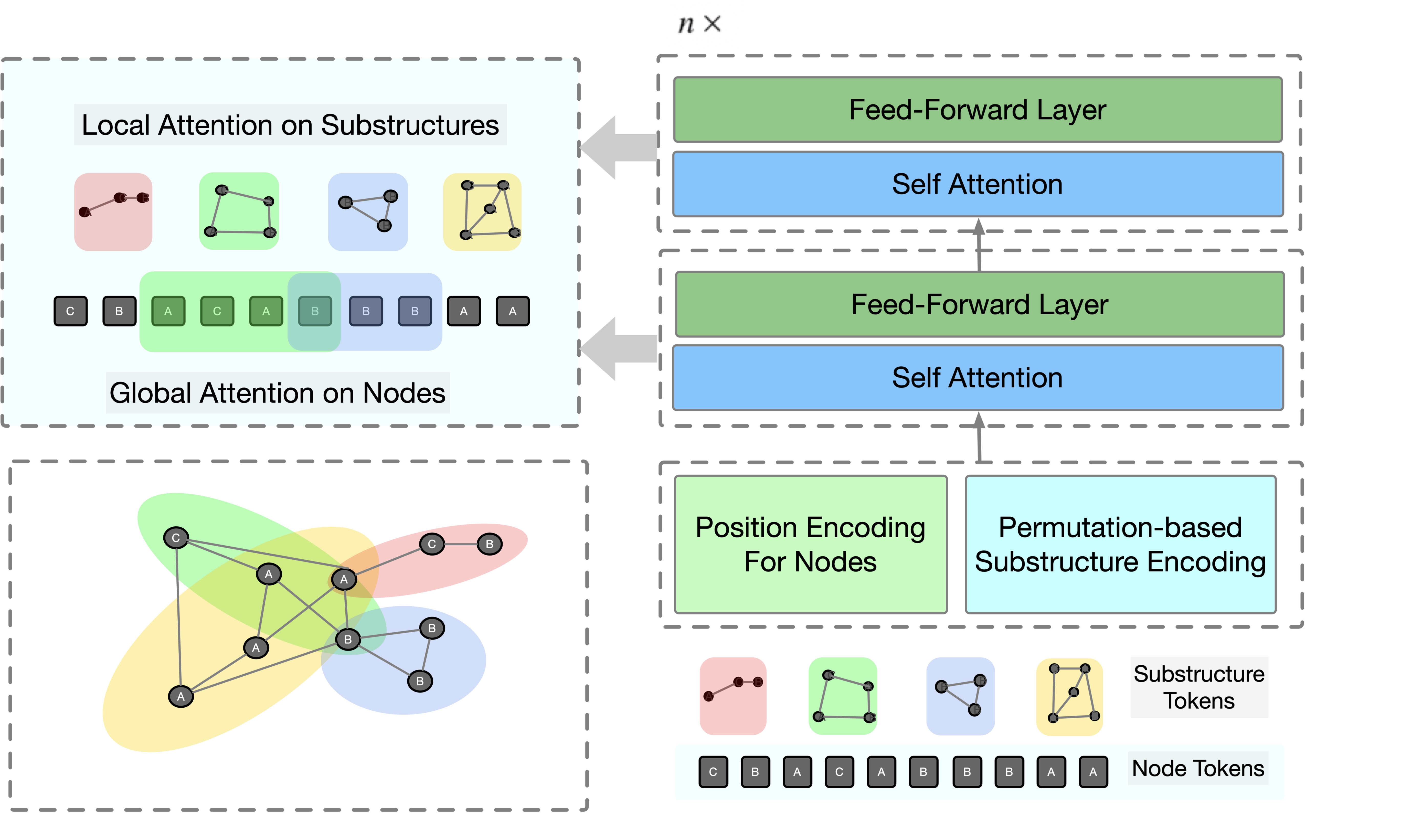
Figure 2: Overview of the proposed graph encoding framework.

4 Theoretical Results

In this section, we study the capacity of global attention to explain the depth bottleneck in graph transformers. The global attention is intended to focus on important substructures and learn expressive substructure representations automatically. However, the fact that graph transformers perform poorly when more layers are stacked raises doubts about the effectiveness of these self-attention layers. The attention layers require sufficient capacity to represent various substructures, which is necessary for learning attention patterns. We define attention capacity, analyze its variation with depth, and propose that local attention to substructures is a potential solution.

4.1 Definition of Attention Capacity

We define the capacity of attention as the maximum difference between representations learned by different substructure attention patterns. Let $\operatorname{supp}(e)$ be all the non-zero dimensions of vector $e$. We define a fixed attention pattern $e$ of substructure $G^{S}$ as an attention vector that only focuses on nodes of $G^{S}$, i.e., ${\operatorname{supp}(e)=N^{S}},\text{ where }e\in[0,1]^{n},e^{T}\textbf{1}=1.$

Given a graph $G$ with several important substructures $G^{S}_{1}\dots G^{S}_{m}$ and corresponding attention patterns $e_{1}\dots e_{m}$, denote $E=(e_{1},e_{2}\dots,e_{m})$ where columns of $E$ are the base vectors of attention patterns on substructures. We consider the attention space spanned by these attention patterns. Attention from this space only focuses on the important substructures:

$$\Delta_{S}\triangleq\{Ec|c\in[0,1]^{m},c^{T}\textbf{1}=1\},$$ (4)

Denote $\Delta^{n}_{S}$ as matrix space with n columns all in space $\Delta_{S}$. We then define attention capacity as the maximum difference between outputs computed by the self-attention with different attention matrices from space $\Delta^{n}_{S}$. Let $\operatorname{\hat{Attn}}_{A}$ be the self-attention mapping where attention matrix equals $A$.

Definition 1

The attention capacity is defined as:

$$F_{H} =\max_{A_{1}^{T},A_{2}^{T}\in\Delta^{n}_{S}}|\operatorname{\hat{Attn}}_{A_{1}}(H)-\operatorname{\hat{Attn}}_{A_{2}}(H)|_{F}$$ (4.1)

$$=\max_{C_{1},C_{2}\in\{C|C\in[0,1]^{m\times n},C^{T}\textbf{1}=\textbf{1}\}}|C_{1}^{T}E^{T}HW^{VO}-C_{2}^{T}E^{T}HW^{VO}|_{F},$$

Attention capacity in graph transformers is crucial. Larger capacity enables varying features by focusing on different substructures, while smaller capacity limits attention patterns’ impact on learned representations. Smaller capacity modules have difficulty learning attention patterns as they are less sensitive to substructures.

4.2 Attention Capacity Decreases with Depth

After defining the measure of attention capacity for substructures, we investigate the attention capacity of graph transformers w.r.t depth both empirically and theoretically. We first empirically demonstrate how the attention capacity in the graph transformer varies with depth, then theoretically analyze the phenomenon and possible solution.

The attention capacity of deep graph transformers for various substructures is computed per Definition 4.1 and normalized by hidden embedding norm (see Appendix G). Figure 1 (right) shows the results. Graphormer (Ying et al., 2021)’s attention capacity decreases significantly after the 24th layer, while SAT (Chen et al., 2022) decreases across all layers, indicating their limitations.

Next, we illustrate that the stacked self-attention layers can cause decreased attention capacity for deeper layers. We first demonstrate that the self-attention module decreases the capacity of attention, then discuss the case with fully-connected layers.

Theorem 1 (The stacked attention modules decrease the capacity of attention)

We analyze capacity of attention $F_{H_{l}}$ for stacked attention modules $H_{i+1}=Attn(H_{i})=(H_{i}+A_{i}H_{i}W_{i}^{VO}-\textbf{1}{b_{i}^{N}}^{T})D_{i}$. Assume $H_{i}W^{VO}_{i}D_{i}$ is full row rank for each layer $i$. Due to the property of layer normalization and properly designed initialization, assume the output of attention module equals to its input, i.e., for input $X$, $|\operatorname{Attn}(X)|_{F}\approx|X|_{F}$. Then the attention capacity of layer l is upper bounded by

$$F_{H_{l}}\leq{\sqrt{2m}}\prod_{i=1}^{l-1}(\alpha_{i})|P_{m}E^{T}|_{2}|W_{l}^{VO}|_{2}|PH_{1}|_{F}$$ (5)

,where $\alpha_{i}=\frac{(|PH_{i}+PA_{i}H_{i}W^{VO}_{i})D_{i}|_{F}}{|(PH_{i}+A_{i}PH_{i}W^{VO}_{i}-\textbf{1}{b_{i}^{N}}^{T})D_{i}|_{F}}<1$ with probability 1, and $P\triangleq(I-\frac{1}{n}\textbf{1}\textbf{1}^{T})$, $P_{m}\triangleq(I-\frac{1}{m}\textbf{1}\textbf{1}^{T})$.

Proof is in Appendix 1. The analysis above reveals that the self-attention module decreases the upper bound of attention capacity exponentially. We next consider the case when fully-connected layers are also included in each layer, just like the architecture in practice.

Theorem 2 (The upper bound of attention capacity after stacked transformer layers)

For transformer layer with self-attention $H_{i}^{\prime}={\operatorname{Attn}}(H_{i})=(H_{i}+A_{i}H_{i}W_{i}^{VO}-\textbf{1}{b_{i}^{N}}^{T})D_{i}$, and fully-connected layer $H_{i+1}=\operatorname{FFN}(H^{\prime}_{i})=(H_{i}^{\prime}+ReLU(H_{i}^{\prime}W_{i}^{F_{1}}+\textbf{1}{b_{i}^{F_{1}}}^{T})W_{i}^{F_{2}}+\textbf{1}{b_{i}^{F_{2}}}^{T}-\textbf{1}{b_{i}^{N_{2}}}^{T})D_{i}^{\prime}$, with the same assumption as the previous, attention capacity of layer $l$ is upper bounded as follows:

$$F_{H_{l}}\leq{\sqrt{2m}}\prod_{i=1}^{l-1}(\alpha_{i}\gamma_{i})|P_{m}E^{T}|_{2}|W_{l}^{VO}|_{2}|PH_{1}|_{F}$$ (6)

,where $\alpha_{i}=\frac{(|PH_{i}+PA_{i}H_{i}W^{VO}_{i})D_{i}|_{F}}{|(PH_{i}+A_{i}PH_{i}W^{VO}_{i}-\textbf{1}{b_{i}^{N}}^{T})D_{i}|_{F}}<1$ with probability 1, and $\gamma_{i}=|D_{i}^{\prime}|_{2}(1+|W_{i}^{F_{1}}|_{2}|W_{i}^{F_{2}}|_{2})$.

Proof in Appendix 2. Fully-connected layer impact can be bounded by coefficients $\gamma_{i}$, which describe hidden embedding norm change. Previous work Shi et al. (2021) shows that $\gamma_{i}$ is dominated by $|D_{i}^{\prime}|_{2}$, and for a fraction of data $|D_{i}^{\prime}|_{2}<1$, leading to attention capacity vanishing in these cases.

4.3 Local Attention for Deep Model

Reducing attention capacity with depth creates two problems for graph transformers: difficulty attending to substructures and loss of feature expressiveness to substructures. To address the first problem, it’s natural to introduce substructure-based local attention as inductive bias into graph transformer to make up for the deficiency of attention on substructures, where each node can only attend to other nodes that belong to same substructures. Furthermore, We will next show that introducing substructures based local attention also addresses the second problem. We next prove that capacity decay can be alleviated if local attention to substructures is applied in each layer.

Theorem 3

Define substructure based local attention as where each node only attends nodes that belong to the same substructures. Assume that for each node, the number of nodes belonging to the same substructures is at most $r$, where $r<n$. Let $\alpha^{s}$ be the decay coefficient of this model in Theorem 1, and $\alpha$ be the decay coefficient of the global attention model. Denoted minimum of $\alpha^{s}$ and $\alpha$ for all possible representation $H_{i}$ and model parameters by ${\alpha^{s}}^{*}$ and $\alpha^{*}$ respectively. Then we have ${\alpha^{s}}^{*}>\alpha^{*}$.

The proof is in Appendix 3. This theory illustrates that substructure based local attention not only introduces the substructure based attention to encourage the model to focus on substructure features but also enlarges the attention capacity of deep layers, which promotes the representation capacity of the model when it grows deep.

5 Approach

Replacing global attention directly with local attention may lead to insufficient learning ability of the model for long-range dependencies. To better introduce local attention to substructure in self-attention models, we propose a novel substructure token based local attention method, DeepGraph, as Figure 2 shows. DeepGraph tokenizes the graph into node level and substructure level. Local attention is applied to the substructure token and corresponding nodes, while the global attention between nodes is still preserved. This provides a better solution for explicitly introducing attention to substructures in the model while combining global attention, to achieve a better global-local encoding balance.

Our method first samples substructures of the graph, then encodes substructures into tokens, and finally enforces local attention on substructures.

5.1 Substructure Sampling

As we aim to stress critical substructures in graph, there are numerous types of substructures that are categorized into two groups: neighbors containing local features, such as k-hop neighbors Zhang & Li (2021) and random walk neighbors Zhao et al. (2021), and geometric substructures representing graph topological features, such as circles Bodnar et al. (2021), paths, stars, and other special subgraphs Bouritsas et al. (2022). We integrate these substructures into a unified substructure vocabulary in this work. In order to match geometric substructures, we use the Python package graph-tool that performs efficient subgraph matching. It is practical to pre-compute these substructures once, and then cache them for reuse. It takes about 3 minutes to compute all the substructures of ZINC, and about 2 hours for PCQM4M-LSC.

Substructures in a graph often exceed the number of nodes. In order to ensure the feasibility of the computation, we sample substructures in each computation. Formally, at each time of encoding, for a graph $G$ with the corresponding substructure set $\{G^{S}\}$, we sample a subset $\{G^{S}_{1},G^{S}_{2}\dots G^{S}_{m}\}$ as input to our model:

$$\{G^{S}_{1},G^{S}_{2}\dots G^{S}_{m}\} =\operatorname{SubstructureSampling}(\{G^{S}\}),$$ (7)

$$\hat{y} =\operatorname{DeepGraph}(G,\{G^{S}_{1},G^{S}_{2}\dots G^{S}_{m}\})$$

We hope the sampled substructures cover every node of the graph as evenly as possible (Zhao et al., 2021) in order to reduce biases resulting from the uneven density of substructures. We also balance the types of substructures in our sampling, due to the divergent ratios of different substructure types in a graph. The details are in Appendix C and D.

5.2 Substructure Token Encoding

The input embedding contains node tokens embedding $\{h_{1},h_{2},\dots,h_{n}\}$ and substructure tokens embedding $\{h_{n+1},\dots,h_{n+m}\}$, encoded by node feature encoder $g_{n}$ and substructure encoder $g_{s}$ individually. The token embedding of graph nodes is mapped from graph node feature $x$ to feature vector $h$: $h_{i}=g_{n}(x_{i}),i\in\{1,2,\dots n\}$.

For the substructure tokens, we apply permutation-based structure encoding (Murphy et al., 2019; Chen et al., 2020b; Nikolentzos & Vazirgiannis, 2020) by encoding the substructure adjacency matrix $\mathbf{A^{S}_{i}}$ directly. The core idea of permutation-based encoding is pooling the encoding output of permuted graph information over all the possible permutations, which is permutation-invariant and has no information loss. We further apply depth-first search (DFS) with the order of node degree to reduce the possible order of substructure nodes. At the beginning and at each step of DFS, we use degrees to sort nodes. A random node from the ones with the least degree is selected as the starting point for DFS. The nodes are sorted according to their degree at each DFS step, while the same-degree nodes are randomly permuted. See Appendix E for more details. Using this method, the graph encoding permutations is invariant and the number of possible combinations is greatly reduced. The formal definition of substructure token encoder is

$$h_{n+i}=\mathop{Pool}\limits_{\pi\in\operatorname{DFS}(\mathbf{A^{S}_{i}})}g_{s}(\pi(\mathbf{A^{S}_{i}})),i\in\{1,2,\dots m\}$$ (8)

In practice, sampling is applied instead of pooling. A single sample is sufficient during training to allow the model to learn the substructure stably.

5.3 Local Attention on Substructures

The substructure and its corresponding nodes receive localized attention after substructure tokens have been added. Given input embedding $H_{1}=(h_{1},h_{2},\dots,h_{n+m})$, mask $M$ is added in self-attention module $\hat{\operatorname{Attn_{m}}}(H,M)$ as

$$\hat{\operatorname{Attn_{m}}}(H_{l},M)=\operatorname{softmax}(\hat{A}+M)H_{l}W^{VO},$$ (9)

where $M_{ij}\in\{0,-\infty\}$, i.e., the elements of mask $M$ can be $0$ or $-\infty$, leading to a sparse attention matrix $A$ with zero in position of $-\infty$ in $M$. In our model, the mask is defined as follows to induce local attention to substructure tokens and corresponding nodes: $M_{ij}=-\infty$ if $i+n\in\{n+1,n+2,\dots n+m\},j\not\in N^{S}_{i}$ or $j+n\in\{n+1,n+2,\dots n+m\},i\not\in N^{S}_{j}$, and $M_{ij}=0$ otherwise. The substructure tokens only apply local attention to corresponding nodes.

The attention in our model is a combination of local attention on substructures and global attention. Substructure tokens are the core of local attention, attending only to corresponding nodes, and integrating representation from the whole substructure. Nodes belonging to the same substructure share a substructure token message, increasing distinguishability of substructures and promoting substructure representation capacity.

6 Experiments

In this section, we aim to validate the performance of DeepGraph empirically. Specifically, we attempt to answer the following questions: (i) How does DeepGraph perform in comparison to existing transformers on popular benchmarks? (ii) Does DeepGraph’s performance improve with increasing depth? (iii) Is DeepGraph capable of alleviating the problem of shrinking attention capacity? (IV) What is the impact of each part of the model on overall performance? We first conduct experiments to evaluate our model on four popular graph datasets, comparing it with state-of-the-art graph transformer models, as well as their augmented deeper versions. Then we illustrate the attention capacity of DeepGraph by visualization. Finally, we validate the effect of different components through ablation studies. Codes are available at https://github.com/zhao-ht/DeepGraph.

6.1 Datasets

Our method is validated on the tasks of the graph property prediction and node classification, specifically including PCQM4M-LSC (Hu et al., 2020), ZINC (Dwivedi et al., 2020), CLUSTER (Dwivedi et al., 2020) and PATTERN (Dwivedi et al., 2020), widely used in graph transformer studies. PCQM4M-LSC is a large-scale graph-level regression dataset with more than 3.8M molecules. ZINC consists of 12,000 graphs with a molecule property for regression. CLUSTER and PATTERN are challenging node classification tasks with graph sizes varying from dozens to hundreds, containing 14,000 and 12,000 graphs, respectively.

6.2 Baselines

We choose recent state-of-art graph transformer models: GT (Dwivedi & Bresson, 2020), SAN (Kreuzer et al., 2021), Graphormer (Ying et al., 2021) and SAT (Chen et al., 2022), covering various graph transformer methods including absolute and relative position embedding. Graph neural networks baselines includes GCN (Kipf & Welling, 2016) and GIN (Xu et al., 2018a). We first compare our model with the standard state-of-art models. Then we compare our model with the deepened state-of-arts augmented by recent algorithms for deep transformers, including the fusion method (Shi et al., 2021), and reattention method (Zhou et al., 2021). As we use deepnorm to stabilize our training process, we compare DeepGraph to naive deepnorm in the ablation study.

6.3 Settings

We implement DeepGraph with 12, 24, and 48 layers. The hidden dimension is 80 for ZINC and PATTERN, 48 for CLUSTER, and 768 for PCQM4M-LSC. The training uses Adam optimizer, with warm-up and decaying learning rates. Reported results are the average of over 4 seeds. Both geometric substructure and neighbors are used as substructure patterns in our model. We imply both geometric substructures and k-hop neighbors on ZINC and PCQM4M-LSC. As for CLUSTER and PATTERN, only random walk neighbors are used due to the large scale and dense connection of these two datasets. The effect of different substructure patterns is shown in the ablation study.

6.4 Main Results

Table 1 summarizes our experimental results on the graph regression and node classification tasks. The data for the baseline models are taken from their papers. The depth of our model varies from 12 to 48 layers. As the results illustrated, our 12-layer model outperforms baseline models on PCQM4M-LSC, ZINC, and PATTERN, especially on ZINC and PATTERN, surpassing the previous best result reported significantly. As model depth increases, our model achieves consistent improvement. Note that our model with 48 layers outperforms baseline models on all the datasets, proving the effectiveness of more stacked DeepGraph layers. The parameter number of each model for each dataset is provided in Appendix H.

	Graph regression		Node classification
PCQM4M-LSC $\downarrow$	ZINC $\downarrow$	CLUSTER $\uparrow$	PATTERN $\uparrow$
GCN	0.1691	0.367 $\pm$ 0.011	68.498 $\pm$ 0.976	71.892 $\pm$ 0.334
GIN	0.1537	0.526 $\pm$ 0.051	64.716 $\pm$ 1.553	85.387 $\pm$ 0.136
GT-sparse	-	0.226 $\pm$ 0.014	73.169 $\pm$ 0.622	84.808 $\pm$ 0.068
GT-Full	-	0.598 $\pm$ 0.049	27.121 $\pm$ 8.471	56.482 $\pm$ 3.549
SAN-Sparse	-	0.198 $\pm$ 0.004	75.738 $\pm$ 0.106	81.329 $\pm$ 2.150
SAN-Full	-	0.139 $\pm$ 0.006	76.691 $\pm$ 0.247	86.581 $\pm$ 0.037
Graphormer	0.1234	0.122 $\pm$ 0.006	-	-
SAT	-	0.094 $\pm$ 0.008	77.856 $\pm$ 0.104	86.865 $\pm$ 0.043
DeepGraph (12)	0.1220	0.078 $\pm$ 0.006	77.526 $\pm$ 0.122	90.015 $\pm$ 0.038
DeepGraph (24)	0.1206	0.076 $\pm$ 0.004	77.810 $\pm$ 0.167	90.522 $\pm$ 0.059
DeepGraph (48)	0.1193	0.072 $\pm$ 0.004	77.912 $\pm$ 0.138	90.657 $\pm$ 0.062

Table 1: Comparison of our DeepGraph to SOTA methods on graph regression and node classification tasks.

6.5 Effect of Deepening

We next compare DeepGraph with other deepened baseline models. We choose Graphormer and SAT as baseline models, and we deepen them by 2 and 4 times compared to the original version. Along with deepening naively, we also enhance baseline models through the fusion method and reattention method.

	DeepGraph 12		DeepGraph 48
	ZINC	CLUSTER	ZINC	CLUSTER
- local attention	0.135	76.167	0.141	76.133
- substructure encoding	0.085	76.531	0.124	77.884
- deepnorm	0.080	77.202	0.074	77.682
DeepGraph	0.078	77.526	0.072	77.912

Table 2: Ablation study of local attention, substructure encoding, and deepnorm on ZINC and CLUSTER.

	DeepGraph 12	DeepGraph 48
Geometric only	0.078	0.075
Neighbors only	0.086	0.079
Both	0.078	0.072

Table 3: Sensitivity study of different substructure types on ZINC.

As shown in Figure 3, DeepGraph outperforms baselines by a significant margin. Naive deepening decreases performance on all the datasets for both baseline models. Note that all the 4-time deep SAT fail to converge on CLUSTER due to the training difficulty, as well as Graphormer with reattention. Fusion improves deeper Graphormer on PCQM4M-LSC, and reattention boosts 2x deep SAT on CLUSTER slightly, but none of them are consistent. Our methods surpass fusion and reattention methods stably on all 4 datasets, supporting our theoretical claim that sensitivity to substructures is crucial in deep graph transformers.

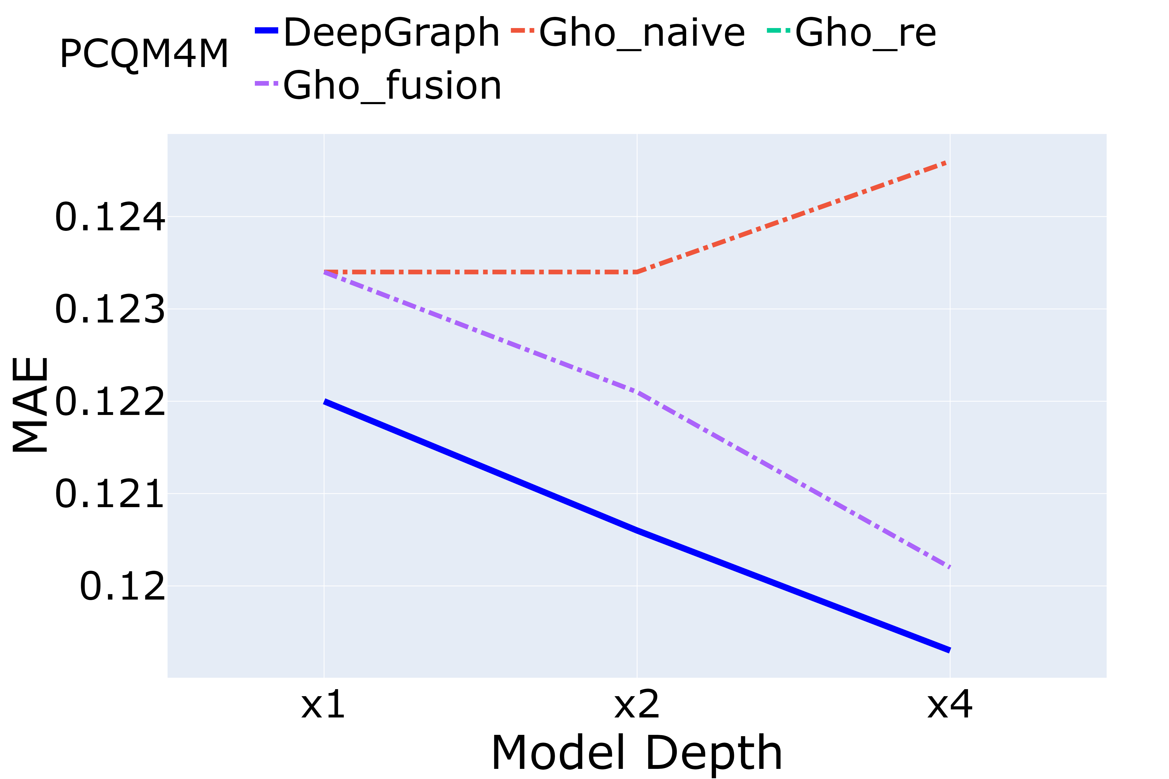
(a)

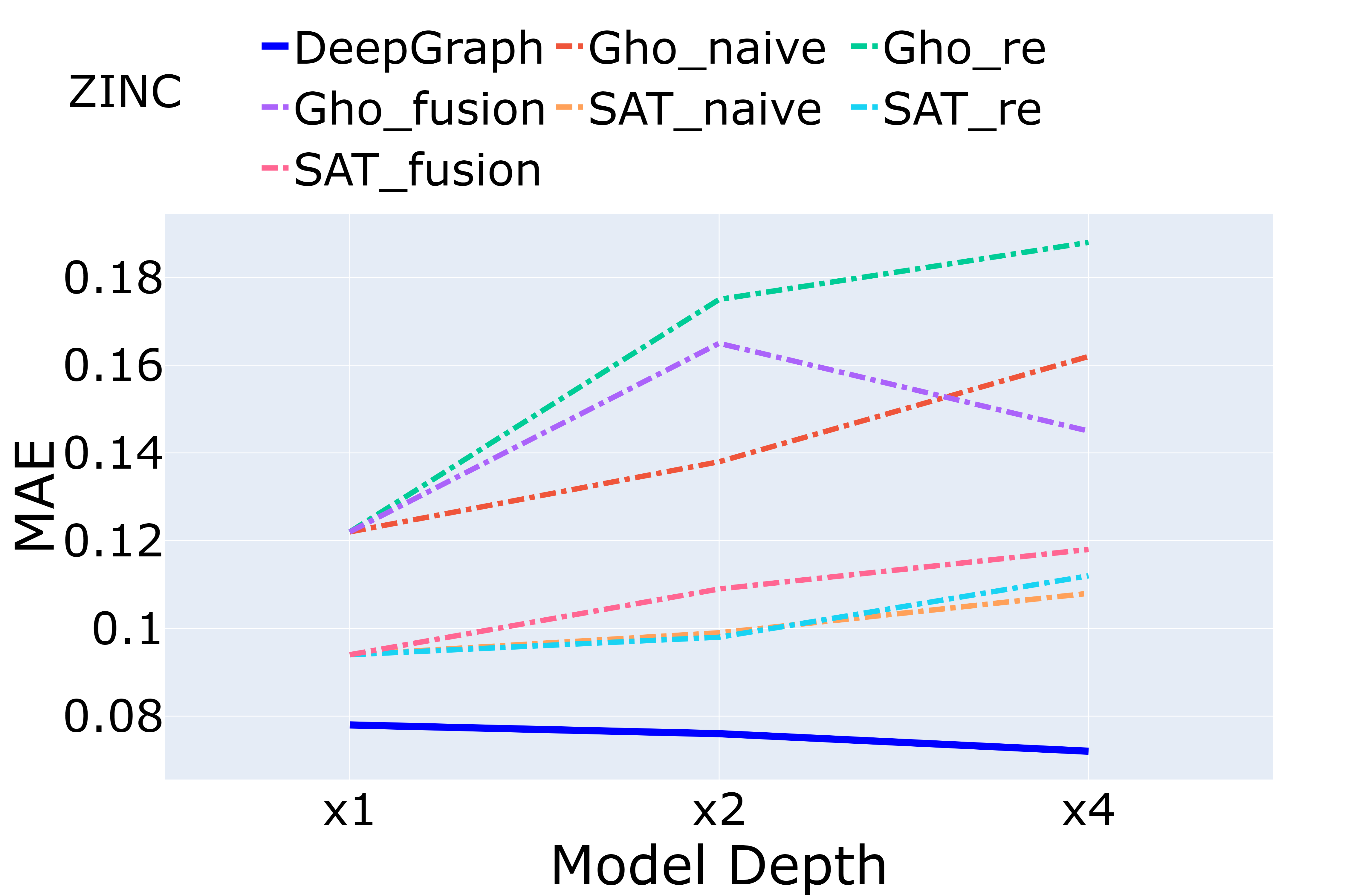
(b)

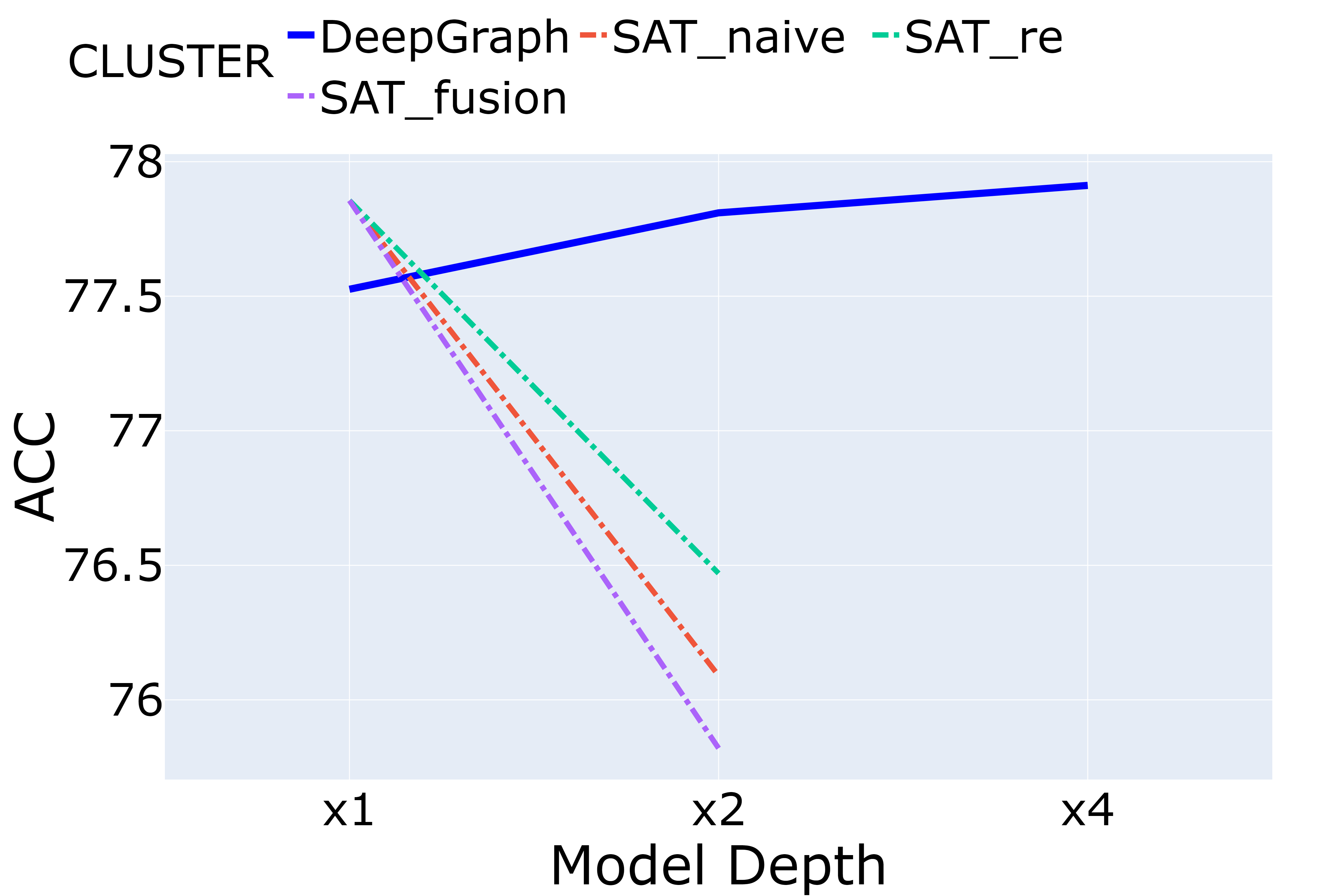
(c)

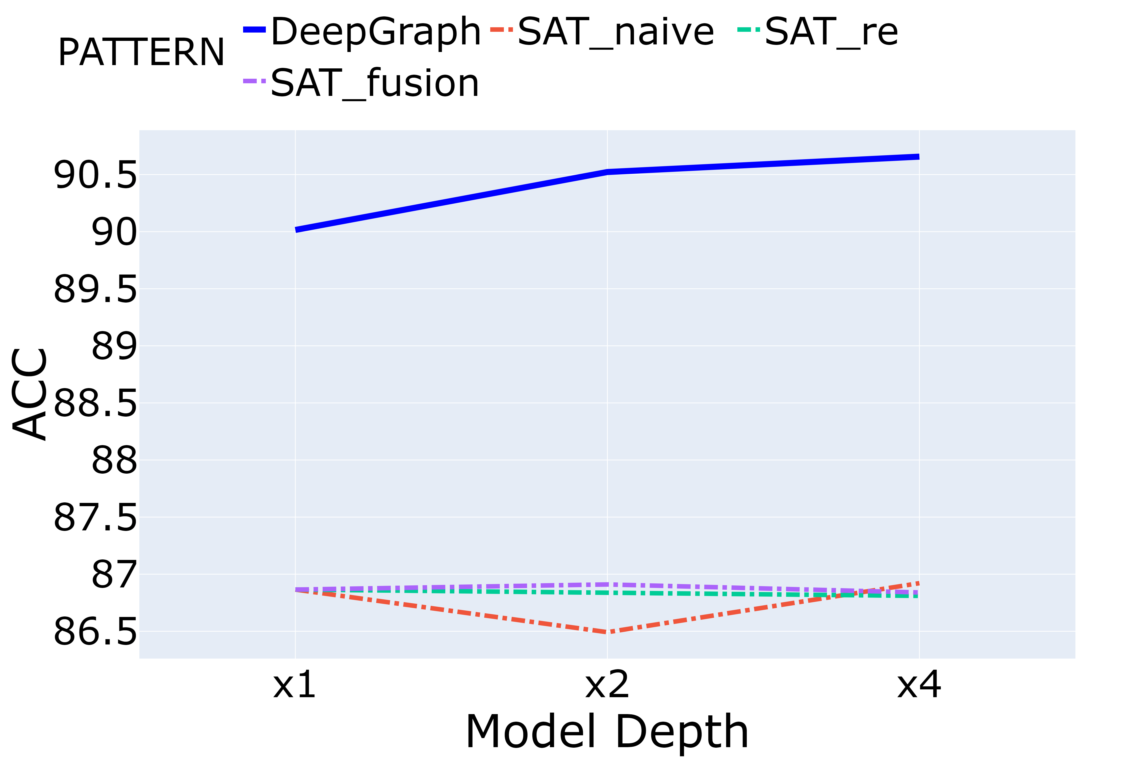
(d)

Figure 3: Comparison of DeepGraph to SOTA methods deepened by different deep transformer methods.

6.6 Visualization of Attention Capacity

We visualize attention capacity of our method and deep baselines on ZINC dataset, using the same substructures as our model. Additionally, to illustrate the capacity of token representation of substructures, we also directly compute the maximum difference between all the substructure tokens value vectors. All the results are normalized by the corresponding representation norm. See Appendix G for details. The results are plotted in Figure 1 (right).

First, the attention capacity of our model remains high across all layers as compared to baselines, indicating that substructure-based local attention can be a useful method for preventing attention deficits. Second, substructure tokens have a much higher capacity than attention capacity computed on nodes, demonstrating the benefits of using substructure tokens for substructure encoding.

6.7 Ablation and Sensitivity Study

Finally, we verify our model’s effectiveness through an ablation study on ZINC and CLUSTER tasks, removing local attention, substructure encoding, and deepnorm to observe their impact. Note that without local attention, the model is only a relative position-based graph transformer with deepnorm residual connections. Without substructure encoding, randomly initialized embedding is applied to each substructure token. Results in Table 6.5 show that without local attention, performance decreases significantly on both datasets, especially for deeper models, proving the effectiveness of the proposed methods. Furthermore, substructure encoding also plays an instrumental role, emphasizing the importance of structural information. Finally, deepnorm also contributes to model performance by stabilizing the optimization, especially for 48-layer models.

We validate the sensitivity of our model to different substructure types by testing the performance of DeepGraph with only geometric substructures or neighbors. Table 6.5 indicates that both contribute to performance, but geometric substructures are more critical for ZINC. This result is expected because specific structures like rings are important fundamental features for the molecule data, and it can be further strengthened when combined with neighbor substructures. Our model can flexibly use different forms of substructure to fully utilize prior knowledge of data.

7 Conclusions

This work presents the bottleneck of graph transformers’ performance when depth increases. By empirical and theoretical analysis, we find that deep graph transformers are limited by the capacity bottleneck of graph attention. Furthermore, we propose a novel graph transformer model based on substructure-based local attention with additional substructure tokens. Our model enhances the ability of the attention mechanism to focus on substructures and addresses the limitation of encoding expressive features as the model deepens. Experiments show that our model breaks the depth bottleneck and achieves state-of-the-art performance on popular graph benchmarks.

Appendix A Proof of Theorems

Proof 1

for brevity, define $P\triangleq(I-\frac{1}{n}\textbf{1}\textbf{1}^{T})$, and $P_{m}\triangleq(I-\frac{1}{m}\textbf{1}\textbf{1}^{T})$. We first introduce an important property of $P$: For any matrix $B$ with left eigenvector $B\textbf{1}=\beta\textbf{1}$, we have $PBC$=$PBPC,\forall C$. To prove it, we can deompose $C=PC+\frac{1}{n}\textbf{1}\textbf{1}^{T}C$. Then

$$PBC=PB(PC+\frac{1}{n}\textbf{1}\textbf{1}^{T}C)=PBPC+\beta\frac{1}{n}P\textbf{1}\textbf{1}^{T}C=PBPC$$

We next prove the main theorem by recursion. By definition,

$$F_{H} =\max_{A_{1}^{T},A_{2}^{T}\in\Delta^{n}_{S}}|\hat{Attn}_{A_{1}}(H)-\hat{Attn}_{A_{2}}(H)|_{F}$$ (10)

$$=\max_{C_{1},C_{2}\in\{C|C\in[0,1]^{m\times n},C^{T}\textbf{1}=\textbf{1}\}}|C_{1}^{T}E^{T}HW^{VO}-C_{2}^{T}E^{T}HW^{VO}|_{F}$$

$$=\max_{C_{1},C_{2}\in\{C|C\in[0,1]^{m\times n},C^{T}\textbf{1}=\textbf{1}\}}|(C_{1}-C_{2})^{T}E^{T}HW^{VO}|_{F}$$

Note that $(C_{1}-C_{2})^{T}\textbf{1}=\textbf{1}-\textbf{1}=0$, so we can multiply $P_{m}$ before it:

$$F_{H} =\max_{C_{1},C_{2}\in\{C|C\in[0,1]^{m\times n},C^{T}\textbf{1}=\textbf{1}\}}|(C_{1}-C_{2})^{T}E^{T}HW^{VO}|_{F}$$ (11)

$$=\max_{C_{1},C_{2}\in\{C|C\in[0,1]^{m\times n},C^{T}\textbf{1}=\textbf{1}\}}|(C_{1}-C_{2})^{T}P_{m}E^{T}HW^{VO}|_{F}$$

$$\leq\max_{C_{1},C_{2}\in\{C|C\in[0,1]^{m\times n},C^{T}\textbf{1}=\textbf{1}\}}|(C_{1}-C_{2})^{T}|_{2}|P_{m}E^{T}HW^{VO}|_{F}$$

$$\leq{\sqrt{2m}}|P_{m}E^{T}HW^{VO}|_{F}$$

,where $|(C_{1}-C_{2})^{T}|_{2}\leq\sqrt{|(C_{1}-C_{2})^{T}|_{1}|(C_{1}-C_{2})^{T}|_{\infty}}=\sqrt{2m}$.

We further decompose $|P_{m}E^{T}HW^{VO}|_{F}$ into

$$|P_{m}E^{T}HW^{VO}|_{F}=|P_{m}E^{T}PHW^{VO}|_{F}\leq|P_{m}E^{T}|_{2}|W^{VO}|_{2}|PH|_{F}$$ (12)

For layer $l$, we recursively compute $|PH_{i+1}|_{F}$ by $|PH_{i}|_{F}$ for layer $i=l-1,l-2,\dots,1$:

$$|PH_{i+1}|_{F} =|P(H_{i}+A_{i}H_{i}W^{VO}_{i}-\textbf{1}{b_{i}^{N}}^{T})D_{i}|_{F}$$ (13)

$$=|P(PH_{i}+A_{i}PH_{i}W^{VO}_{i}-\textbf{1}{b_{i}^{N}}^{T})D_{i}|_{F}$$

$$=\frac{|P(PH_{i}+A_{i}PH_{i}W^{VO}_{i}-\textbf{1}{b_{i}^{N}}^{T})D_{i}|_{F}}{|(PH_{i}+A_{i}PH_{i}W^{VO}_{i}-\textbf{1}{b_{i}^{N}}^{T})D_{i}|_{F}}\frac{|(PH_{i}+A_{i}PH_{i}W^{VO}_{i}-\textbf{1}{b_{i}^{N}}^{T})D_{i}|_{F}}{|PH_{i}|_{F}}|PH_{i}|_{F}$$

$$=\alpha_{i}\lambda_{i}|PH_{i}|_{F}$$

,where $\alpha_{i}=\frac{|P(PH_{i}+A_{i}PH_{i}W^{VO}_{i}-\textbf{1}{b_{i}^{N}}^{T})D_{i}|_{F}}{|(PH_{i}+A_{i}PH_{i}W^{VO}_{i}-\textbf{1}{b_{i}^{N}}^{T})D_{i}|_{F}}$, and $\lambda_{i}=\frac{|(PH_{i}+A_{i}PH_{i}W^{VO}_{i}-\textbf{1}{b_{i}^{N}}^{T})D_{i}|_{F}}{|PH_{i}|_{F}}$.

Note that $P=(I-\frac{1}{n}\textbf{1}\textbf{1}^{T})$ is a contraction mapping, so $\alpha_{i}\leq 1$, and equal to 1 if and only if $A_{i}PH_{i}W^{VO}_{i}D_{i}-\textbf{1}{b_{i}^{N}}^{T}D_{i}$ is orthogonal to the 1-stretched space, which is usually impossible, because $-\textbf{1}{b_{i}^{N}}^{T}D_{i}$ is in the 1-stretched space, and the probability that projection of $A_{i}PH_{i}W^{VO}_{i}D_{i}$ on 1-stretched space equals to $\textbf{1}{b_{i}^{N}}^{T}D_{i}$ is 0 due to the property of random matrix. We further show that $A_{i}PH_{i}W^{VO}D_{i}$ is full-rank with probability 1: As assumption, $H_{i}W^{VO}_{i}D_{i}$ is full-rank, and 1-stretched space is the only subspace that $PH_{i}W^{VO}_{i}D_{i}$ is orthogonal to, i.e.

$$x^{T}PH_{i}W^{VO}_{i}D_{i}=0\Leftrightarrow x=\beta\textbf{1}$$

. So if $\textbf{1}^{T}A_{i}PH_{i}W^{VO}_{i}D_{i}=0$, $\textbf{1}^{T}A_{i}=\beta\textbf{1}^{T}$, i.e. $A_{i}^{T}\textbf{1}=\beta\textbf{1}$, the probability of which is 0 for random parameters in transformer.

For coefficient $\lambda_{i}$, due to the property of layer normalization and good parameter initialization that keeps norm of output equals to input, i.e. $|(X+A_{i}XW^{VO}_{i}-\textbf{1}{b_{i}^{N}})D_{i}|_{F}/|X|_{F}\approx 1,\forall X$, we have $\lambda\approx 1$.

Based on the analysis above, we can bound $F_{H_{l}}$ recursively:

$$F_{H_{l}}\leq{\sqrt{2m}}\prod_{i=1}^{l-1}(\alpha_{i})|P_{m}E^{T}|_{2}|W_{l}^{VO}|_{2}|PH_{1}|_{F}$$ (14)

, where $\alpha_{i}=\frac{|P(PH_{i}+A_{i}PH_{i}W^{VO}_{i}-\textbf{1}{b_{i}^{N}}^{T})D_{i}|_{F}}{|(PH_{i}+A_{i}PH_{i}W^{VO}_{i}-\textbf{1}{b_{i}^{N}}^{T})D_{i}|_{F}}=\frac{(|PH_{i}+PA_{i}H_{i}W^{VO}_{i})D_{i}|_{F}}{|(PH_{i}+A_{i}PH_{i}W^{VO}_{i}-\textbf{1}{b_{i}^{N}}^{T})D_{i}|_{F}}<1$ with probability 1.

Proof 2

As the same method in the previous proof, we need to recursively bound $|PH_{i+1}|_{F}$ by $|PH_{i}|_{F}$ for layer $i=l-1,l-2,\dots,1$. Deote $H^{\prime}_{i}=\operatorname{Attn}(H_{i})$, and $H_{i+1}=\operatorname{FFN}(H^{\prime}_{i})$. Similar to the previous proof, we have

$$|PH^{\prime}_{i}|_{F} =|P(H_{i}+A_{i}H_{i}W^{VO}_{i}-\textbf{1}{b_{i}^{N}}^{T})D_{i}|_{F}$$ (15)

$$=|P(PH_{i}+A_{i}PH_{i}W^{VO}_{i}-\textbf{1}{b_{i}^{N}}^{T})D_{i}|_{F}$$

$$=\frac{|P(PH_{i}+A_{i}PH_{i}W^{VO}_{i}-\textbf{1}{b_{i}^{N}}^{T})D_{i}|_{F}}{|(PH_{i}+A_{i}PH_{i}W^{VO}_{i}-\textbf{1}{b_{i}^{N}}^{T})D_{i}|_{F}}\frac{|(PH_{i}+A_{i}PH_{i}W^{VO}_{i}-\textbf{1}{b_{i}^{N}}^{T})D_{i}|_{F}}{|PH_{i}|_{F}}|PH_{i}|_{F}$$

$$=\alpha_{i}\lambda_{i}|PH_{i}|_{F}$$

As for $PH_{i+1}$, we can bound it as

$$|PH_{i+1}|_{F} =|P(H_{i}^{\prime}+ReLU(H_{i}^{\prime}W_{i}^{F_{1}}+\textbf{1}{b_{i}^{F_{1}}}^{T})W_{i}^{F_{2}}+\textbf{1}{b_{i}^{F_{2}}}^{T}-\textbf{1}{b_{i}^{N_{2}}}^{T})D^{\prime}_{i}|_{F}$$ (16)

$$=|PH_{i}^{\prime}D_{i}^{\prime}|_{F}+|PReLU(H_{i}^{\prime}W_{i}^{F_{1}}+\textbf{1}{b_{i}^{F_{1}}}^{T})W_{i}^{F_{2}}D_{i}^{\prime}|_{F}$$

$$\leq|PH_{i}^{\prime}|_{F}|D_{i}^{\prime}|_{2}+|PReLU(H_{i}^{\prime}W_{i}^{F_{1}}+\textbf{1}{b_{i}^{F_{1}}}^{T})|_{F}|W_{i}^{F_{2}}|_{2}|D_{i}^{\prime}|_{2}$$

$$\leq|PH_{i}^{\prime}|_{F}|D_{i}^{\prime}|_{2}+|P(H_{i}^{\prime}W_{i}^{F_{1}}+\textbf{1}{b_{i}^{F_{1}}}^{T})|_{F}|W_{i}^{F_{2}}|_{2}|D_{i}^{\prime}|_{2}$$

$$\leq|PH_{i}^{\prime}|_{F}|D_{i}^{\prime}|_{2}+|PH_{i}^{\prime}|_{F}|W_{i}^{F_{1}}|_{2}|W_{i}^{F_{2}}|_{2}|D_{i}^{\prime}|_{2}$$

$$=|D_{i}^{\prime}|_{2}(1+|W_{i}^{F_{1}}|_{2}|W_{i}^{F_{2}}|_{2})|PH_{i}^{\prime}|_{F}$$

So the final conclusion is

$$F_{H_{l}}\leq{\sqrt{2m}}\prod_{i=1}^{l-1}(\alpha_{i}\gamma_{i})|P_{m}E^{T}|_{2}|W_{l}^{VO}|_{2}|PH_{1}|_{F}$$ (17)

, where $\alpha_{i}=\frac{|P(PH_{i}+A_{i}PH_{i}W^{VO}_{i}-\textbf{1}{b_{i}^{N}}^{T})D_{i}|_{F}}{|(PH_{i}+A_{i}PH_{i}W^{VO}_{i}-\textbf{1}{b_{i}^{N}}^{T})D_{i}|_{F}}=\frac{(|PH_{i}+PA_{i}H_{i}W^{VO}_{i})D_{i}|_{F}}{|(PH_{i}+A_{i}PH_{i}W^{VO}_{i}-\textbf{1}{b_{i}^{N}}^{T})D_{i}|_{F}}<1$ with probability 1, and $\gamma_{i}=|D_{i}^{\prime}|_{2}(1+|W_{i}^{F_{1}}|_{2}|W_{i}^{F_{2}}|_{2})$.

Proof 3

We denote global attention and local attention by $A$ and $A^{s}$, respectively.

By definition, $\alpha_{i}=\frac{(|PH_{i}+PA_{i}H_{i}W^{VO}_{i})D_{i}|_{F}}{|(PH_{i}+A_{i}PH_{i}W^{VO}_{i}-\textbf{1}{b_{i}^{N}}^{T})D_{i}|_{F}}$. We analyse the worst case for $\alpha_{i}$:

$$\alpha_{i} =\frac{(|PH_{i}+PA_{i}H_{i}W^{VO}_{i})D_{i}|_{F}}{|(PH_{i}+A_{i}PH_{i}W^{VO}_{i}-\textbf{1}{b_{i}^{N}}^{T})D_{i}|_{F}}$$ (18)

$$=\frac{(|PH_{i}+PA_{i}H_{i}W^{VO}_{i})D_{i}|_{F}}{|(PH_{i}+(P+\frac{1}{n}\textbf{1}\textbf{1}^{T})A_{i}PH_{i}W^{VO}_{i}-\textbf{1}{b_{i}^{N}}^{T})D_{i}|_{F}}$$

$$\geq\frac{(|PH_{i}+PA_{i}H_{i}W^{VO}_{i})D_{i}|_{F}}{|(PH_{i}+PA_{i}H_{i}W^{VO}_{i})D_{i}|_{F}+|\frac{1}{n}\textbf{1}\textbf{1}^{T}A_{i}PH_{i}W^{VO}_{i}D_{i}|_{F}+|\textbf{1}{b_{i}^{N}}^{T}D_{i}|_{F}}$$

Further analysis on $|\frac{1}{n}\textbf{1}\textbf{1}^{T}A_{i}PH_{i}W^{VO}_{i}D_{i}|_{F}$ shows that

$$|\frac{1}{n}\textbf{1}\textbf{1}^{T}A_{i}PH_{i}W^{VO}_{i}D_{i}|_{F} =|\textbf{1}^{T}A_{i}PH_{i}W^{VO}_{i}D_{i}|_{2}$$ (19)

$$\leq|H_{i}W^{VO}_{i}D_{i}|_{2}|PA_{i}^{T}\textbf{1}|_{2},$$

where $PA_{i}^{T}\textbf{1}=A_{i}^{T}\textbf{1}-\textbf{1}$, the element of which is between $[-1,n-1]$, and the sum of all elements of which is 0. The maximum of $|PA_{i}^{T}\textbf{1}|_{2}$ is achieved when one element is $n-1$ and other elements are $-1$.

However, for local attention $A^{s}_{i}$ that each node is only attended by at most r nodes, where $r<n$, the elements of $|P{A_{i}^{s}}^{T}\textbf{1}|_{2}$ is only between $[-1,r-1]$, and thus the maximum $|P{A_{i}^{s}}^{T}\textbf{1}|_{2}$ is less than $|P{A_{i}}^{T}\textbf{1}|_{2}$.

We further address that the two inequalities in 18 and 19 both can be achieved for proper $H_{i}$ and parameters. So we can conclude that for the worst case of $\alpha_{i}$ and ${\alpha_{i}}^{s}$, denoted by ${\alpha_{i}}^{*}$ and ${\alpha_{i}^{s}}^{*}$,

$$\alpha_{i}^{*}<{\alpha_{i}^{s}}^{*}$$

Appendix B Discussion of Substructure Based Attention Space

In Definition 4.1, for a substructure $G^{S}$, the fixed attention pattern $e$ is an ideal attention pattern to help to concentrate on the information of this substructure, for example, a uniform attention vector on a benzene ring, or attention on a two-hop neighbor graph attenuating according to the distance to the central node. Traditional GNN is also an example of such a fixed attention pattern, where each node takes uniform attention to its’ neighbor nodes. Although we treat this pattern as fixed on the substructure, we denote that the definition is general because the value can be any learnable attention pattern.

The defined attention space construct attention patterns for all meaningful attention on substructures by containing the combination of all the elementary substructure pattern. As this substructure attention patterns are considered important indicative bias, the graph transformer is expected to learn attention patterns in this space to utilize the substructure feature. This definition is also general and expressive, as sufficient patterns can be added to include more general cases.

Appendix C Substructures

The sizes of the different substructures used in this study are neighbor substructures including 2-hop neighbor and 10-step random walk neighbor, and geometric substructures including circle with size from 3 to 8, star with size from 2 to 6, and path with size from 4 to 8. For geometric substructures, we use the python package graph-tool for substructure matching. It takes about 3 minutes to match all the geometric substructures of ZINC, and about 2 hours for PCQM4M-LSC. We cache all the substructures for reuse.

Appendix D SubstructureSampling

A greedy sampling algorithm is used for the substructure sampling process. In each step of the iteration, nodes with less coverage have a greater probability of being covered in the next iteration. At the beginning of sampling, we randomly select $n_{init}$ substructures from all the substructures, where different types of substructures are balanced. In each iteration, we first mark nodes as set $N_{left}$ that are covered less than threshold $thre$ times by already sampled substructures. Then we calculate $cnt_{i}$ for each substructure left, which is the number of nodes in $N_{left}$ covered by substructure $G^{S}_{i}$. We select $n_{sample}$ from substructures with top $k$ $cnt$ randomly. The iteration ends when each node is covered at least $thre$ times, or no substructure is left. In the algorithm, $n_{init}$, $k$, and $n_{sample}$ are determined by $thre$ and nodes number to speed up the iteration and increase sampling variance, while retaining that nodes are covered as evenly as possible.

Appendix E Depth-First Search (DFS)

We use degree to sort nodes at the beginning of DFS and each step. In the beginning, DFS start from node uniformly sampled from nodes with the least degree. At each step, nodes are sorted according to degree, while nodes with the same degree are permuted randomly. This method keeps the graph encoding permutation invariant, and reduces possible permutations a lot. The drawback of permutation-based encoding is that the number of possible permutations becomes intractable when the graph is large. Fortunately, the substructure size is usually not larger than 10.

Appendix F Related Work of Token Unit

The most suitable basic unit for transformer as a token has been studied in many works in natural language processing and computational vision. For nature language, sentences are separated into sub-words containing a variant number of primary characters (Kudo & Richardson, 2018). In computational vision, while previous works apply transformer directly on image pixels (Parmar et al., 2018; Hu et al., 2019), recent works find it more beneficial to treat patches as tokens (Dosovitskiy et al., 2020), indicating the importance of proper segmentation of the input. For graph transformers, tokens in most current studies are nodes. We propose to encode substructures together with nodes in the graph as tokens in the transformer.

Appendix G Empirical Study on Attention Capacity

We empirically explore the capacity of the model for the substructure, and validate our theoretical results. We aim to answer the following three questions: (1) Do attention capacity really decreases in deeper graph transformer? (2) Can our method, i.e., local attention with substructure tokens, help to increase model capacity of representing substructures? (3) Can our method, i.e., local attention with substructure tokens, help to alleviate attention capacity decrease?

We visualize the attention capacity of our method and deep baselines on the ZINC dataset. The set of substructures is the same as the substructures used in our model, while the base vectors $E$ are defined as uniform distributions supported on corresponding substructures. Because attention capacity in Definition 4.1 depends on the norm of hidden representations, we normalize it by the norm of all the value vectors $\sum_{i=1\dots n}|h_{i}W^{VO}|_{2}$ to eliminate the influence of the representation norm. Note that for our model, only node tokens are considered. Additionally, because we explicitly tokenize substructures as tokens, we also directly compute the maximum difference between all the substructure tokens value vectors, $\max_{i,j\in\{1\dots m\}}|h_{i+n}W^{VO}-h_{j+n}W^{VO}|_{2}$, and normalize it by $\frac{1}{m}\sum_{i=1\dots m}|h_{i+n}W^{VO}|_{2}$, to illustrate the capacity of token representation of substructures. The results are plotted in Figure 1 (right).

First, the result of Graphormer and SAT reveals that attention capacity of substructures decreases in deep layers. Note that in the shallow layer the attention capacity of Graphormer increases, which is not contradicting our theory because we only claim that the upper bound of attention capacity decrease with depth. However, after the 24th layer, attention capacity decreases a lot, revealing the problem of deepening graph transformer. Note that because SAT uses GNN to encode substructures for query and key computation, it has a high attention capacity in the first layer. However, it decays fast due to the property of global attention.

Second, the result of our model indicates that local attention-based substructure tokens improve substructure representation capacity. The difference between substructure tokens is much larger than the representation learned by attention on substructures, indicating learning substructure token representation by local attention can significantly improve the representation capacity of model, which supports our first motivation that introducing substructure-based local attention help model to encode substructures better.

Finally, compared to baselines, attention capacity of our model remains high across all the layers. Although it drops from 0.96 to 0.90 after the 24th layer, the dropping ratio is smaller than the baseline graph transformer. This supports our claim that substructure-based local attention helps alleviate attention capacity decrease. Note that the capacity of substructure tokens also decreases slower.

Appendix H Parameter Number Comparison

We list parameter numbers of our model and baselines. Note that parameter numbers of Graphormer and SAT are computed by running their official code directly, and other baselines are from papers. The parameter number of SAT (*1) is different from reported in their papers, which may be due to code updates. The parameter number of our base model is comparable to previous works, and even less on CLUSTER. The parameter number of our deeper model is also comparable to deeper baselines, while our performance surpasses them.

	layer	PCQM4M-LSC	ZINC	CLUSTER	PATTERN
GCN	-	2.0M	421k	571k	380k
GIN	-	3.8M	495k	684k	455k
GT-Sparse	-	-	588,929	524,026	522,982
GT-Full	-	-	588,929	524,026	522,982
SAN-Sparse	-	-	494,865	530,036	493,340
SAN-Full	-	-	508,577	519,186	507,202
Graphormer	x1	44,750,081	489,321	-	-
	x2	87,309,569	1,055,985	-	-
	x4	172,428,545	1,996,785	-	-
SAT	x1	-	499,681	741,990	825,986
	x2	-	991,873	1,480,806	1,646,978
	x4	-	1,976,257	2,958,438	3,288,962
Ours	x1	45,563,393	612,705	382,865	612,705
	x2	88,122,881	1,078,225	686,225	1,083,105
	x4	173,241,857	2,019,025	989,585	2,023,905

Appendix I Time Complexity

The time complexity of our methods is mainly due to the larger input size, which increases the cost of transformer. Given graph size $N$ and sampled substructure number $M$, the complexity of transformer is $O((M+N)^{2})$. However, as we use sampling to reduce the substructure number, the substructure number is less than the graph size, i.e. $M<N$, so the complexity will not be more than four times of the standard transformer and remains $O(N^{2})$.

Appendix J Ablation Study on Neighbor Size

We conduct ablation studies for random walk neighbors on CLUSTER and PATTERN datasets. While we use size 10 neighbors in the paper, we compare the performance with sizes 5 and 15. The result is as follows:

	CLUSTER		PATTERN
	12	48	12	48
size 5	77.2	77.7	90.1	90.6
size 15	77.1	78	89.6	90.4
size 10	77.5	77.9	90	90.7

The result shows that the performance remains robust to different substructure sizes, especially the deeper model. Smaller substructures are easy for the model to learn its structure features, but they may not cover enough nodes and provide good graph structure information. Larger substructures are more informative about graph feature, but is more difficult for stable learning, especially for a shallow model.

References

- Alon & Yahav (2020) Uri Alon and Eran Yahav. On the bottleneck of graph neural networks and its practical implications. In International Conference on Learning Representations, 2020.
- Bachlechner et al. (2021) Thomas Bachlechner, Bodhisattwa Prasad Majumder, Henry Mao, Gary Cottrell, and Julian McAuley. Rezero is all you need: Fast convergence at large depth. In Uncertainty in Artificial Intelligence, pp. 1352–1361. PMLR, 2021.
- Bahdanau et al. (2015) Dzmitry Bahdanau, Kyung Hyun Cho, and Yoshua Bengio. Neural machine translation by jointly learning to align and translate. In 3rd International Conference on Learning Representations, ICLR 2015, 2015.
- Bastos et al. (2022) Anson Bastos, Abhishek Nadgeri, Kuldeep Singh, Hiroki Kanezashi, Toyotaro Suzumura, and Isaiah Onando Mulang. Investigating expressiveness of transformer in spectral domain for graphs. arXiv preprint arXiv:2201.09332, 2022.
- Bodnar et al. (2021) Cristian Bodnar, Fabrizio Frasca, Nina Otter, Yuguang Wang, Pietro Lio, Guido F Montufar, and Michael Bronstein. Weisfeiler and lehman go cellular: Cw networks. Advances in Neural Information Processing Systems, 34:2625–2640, 2021.
- Bouritsas et al. (2022) Giorgos Bouritsas, Fabrizio Frasca, Stefanos P Zafeiriou, and Michael Bronstein. Improving graph neural network expressivity via subgraph isomorphism counting. IEEE Transactions on Pattern Analysis and Machine Intelligence, 2022.
- Chen et al. (2022) Dexiong Chen, Leslie O’Bray, and Karsten Borgwardt. Structure-aware transformer for graph representation learning. In International Conference on Machine Learning, pp. 3469–3489. PMLR, 2022.
- Chen et al. (2020a) Ming Chen, Zhewei Wei, Zengfeng Huang, Bolin Ding, and Yaliang Li. Simple and deep graph convolutional networks. In International Conference on Machine Learning, pp. 1725–1735. PMLR, 2020a.
- Chen et al. (2020b) Zhengdao Chen, Lei Chen, Soledad Villar, and Joan Bruna. Can graph neural networks count substructures? Advances in neural information processing systems, 33:10383–10395, 2020b.
- Choromanski et al. (2022) Krzysztof Choromanski, Han Lin, Haoxian Chen, Tianyi Zhang, Arijit Sehanobish, Valerii Likhosherstov, Jack Parker-Holder, Tamas Sarlos, Adrian Weller, and Thomas Weingarten. From block-toeplitz matrices to differential equations on graphs: towards a general theory for scalable masked transformers. In International Conference on Machine Learning, pp. 3962–3983. PMLR, 2022.
- Devlin et al. (2019) Jacob Devlin, Ming-Wei Chang, Kenton Lee, and Kristina Toutanova. Bert: Pre-training of deep bidirectional transformers for language understanding. In Proceedings of the 2019 Conference of the North American Chapter of the Association for Computational Linguistics: Human Language Technologies, Volume 1 (Long and Short Papers), pp. 4171–4186, 2019.
- Dong et al. (2021) Yihe Dong, Jean-Baptiste Cordonnier, and Andreas Loukas. Attention is not all you need: Pure attention loses rank doubly exponentially with depth. In International Conference on Machine Learning, pp. 2793–2803. PMLR, 2021.
- Dosovitskiy et al. (2020) Alexey Dosovitskiy, Lucas Beyer, Alexander Kolesnikov, Dirk Weissenborn, Xiaohua Zhai, Thomas Unterthiner, Mostafa Dehghani, Matthias Minderer, Georg Heigold, Sylvain Gelly, et al. An image is worth 16x16 words: Transformers for image recognition at scale. In International Conference on Learning Representations, 2020.
- Duvenaud et al. (2015) David K Duvenaud, Dougal Maclaurin, Jorge Iparraguirre, Rafael Bombarell, Timothy Hirzel, Alán Aspuru-Guzik, and Ryan P Adams. Convolutional networks on graphs for learning molecular fingerprints. Advances in neural information processing systems, 28, 2015.
- Dwivedi & Bresson (2020) Vijay Prakash Dwivedi and Xavier Bresson. A generalization of transformer networks to graphs. arXiv preprint arXiv:2012.09699, 2020.
- Dwivedi et al. (2020) Vijay Prakash Dwivedi, Chaitanya K Joshi, Thomas Laurent, Yoshua Bengio, and Xavier Bresson. Benchmarking graph neural networks. arXiv preprint arXiv:2003.00982, 2020.
- Guo et al. (2022) Lingbing Guo, Qiang Zhang, and Huajun Chen. Unleashing the power of transformer for graphs. arXiv preprint arXiv:2202.10581, 2022.
- He et al. (2016a) Kaiming He, Xiangyu Zhang, Shaoqing Ren, and Jian Sun. Deep residual learning for image recognition. In Proceedings of the IEEE conference on computer vision and pattern recognition, pp. 770–778, 2016a.
- He et al. (2016b) Kaiming He, Xiangyu Zhang, Shaoqing Ren, and Jian Sun. Identity mappings in deep residual networks. In European conference on computer vision, pp. 630–645. Springer, 2016b.
- Hu et al. (2019) Han Hu, Zheng Zhang, Zhenda Xie, and Stephen Lin. Local relation networks for image recognition. In Proceedings of the IEEE/CVF International Conference on Computer Vision, pp. 3464–3473, 2019.
- Hu et al. (2020) Weihua Hu, Matthias Fey, Marinka Zitnik, Yuxiao Dong, Hongyu Ren, Bowen Liu, Michele Catasta, and Jure Leskovec. Open graph benchmark: Datasets for machine learning on graphs. Advances in neural information processing systems, 33:22118–22133, 2020.
- Jiang et al. (2010) Chuntao Jiang, Frans Coenen, and Michele Zito. Finding frequent subgraphs in longitudinal social network data using a weighted graph mining approach. In International Conference on Advanced Data Mining and Applications, pp. 405–416. Springer, 2010.
- Jin et al. (2018) Wengong Jin, Regina Barzilay, and Tommi Jaakkola. Junction tree variational autoencoder for molecular graph generation. In International conference on machine learning, pp. 2323–2332. PMLR, 2018.
- Jin et al. (2019) Wengong Jin, Regina Barzilay, and Tommi Jaakkola. Hierarchical graph-to-graph translation for molecules. arXiv preprint arXiv:1907.11223, 2019.
- Kim et al. (2022) Jinwoo Kim, Tien Dat Nguyen, Seonwoo Min, Sungjun Cho, Moontae Lee, Honglak Lee, and Seunghoon Hong. Pure transformers are powerful graph learners. arXiv preprint arXiv:2207.02505, 2022.
- Kipf & Welling (2016) Thomas N Kipf and Max Welling. Semi-supervised classification with graph convolutional networks. arXiv preprint arXiv:1609.02907, 2016.
- Koyutürk et al. (2004) Mehmet Koyutürk, Ananth Grama, and Wojciech Szpankowski. An efficient algorithm for detecting frequent subgraphs in biological networks. Bioinformatics, 20(suppl_1):i200–i207, 2004.
- Kreuzer et al. (2021) Devin Kreuzer, Dominique Beaini, Will Hamilton, Vincent Létourneau, and Prudencio Tossou. Rethinking graph transformers with spectral attention. Advances in Neural Information Processing Systems, 34:21618–21629, 2021.
- Kudo & Richardson (2018) Taku Kudo and John Richardson. Sentencepiece: A simple and language independent subword tokenizer and detokenizer for neural text processing. In Proceedings of the 2018 Conference on Empirical Methods in Natural Language Processing: System Demonstrations, pp. 66–71, 2018.
- Li et al. (2019) Guohao Li, Matthias Muller, Ali Thabet, and Bernard Ghanem. Deepgcns: Can gcns go as deep as cnns? In Proceedings of the IEEE/CVF international conference on computer vision, pp. 9267–9276, 2019.
- Li et al. (2020) Guohao Li, Chenxin Xiong, Ali Thabet, and Bernard Ghanem. Deepergcn: All you need to train deeper gcns. arXiv preprint arXiv:2006.07739, 2020.
- Li et al. (2021) Guohao Li, Matthias Müller, Bernard Ghanem, and Vladlen Koltun. Training graph neural networks with 1000 layers. In International conference on machine learning, pp. 6437–6449. PMLR, 2021.
- Li et al. (2018) Qimai Li, Zhichao Han, and Xiao-Ming Wu. Deeper insights into graph convolutional networks for semi-supervised learning. In Thirty-Second AAAI conference on artificial intelligence, 2018.
- Liu et al. (2020a) Liyuan Liu, Xiaodong Liu, Jianfeng Gao, Weizhu Chen, and Jiawei Han. Understanding the difficulty of training transformers. In 2020 Conference on Empirical Methods in Natural Language Processing, EMNLP 2020, pp. 5747–5763. Association for Computational Linguistics (ACL), 2020a.
- Liu et al. (2020b) Meng Liu, Hongyang Gao, and Shuiwang Ji. Towards deeper graph neural networks. In Proceedings of the 26th ACM SIGKDD international conference on knowledge discovery & data mining, pp. 338–348, 2020b.
- Liu et al. (2019) Yinhan Liu, Myle Ott, Naman Goyal, Jingfei Du, Mandar Joshi, Danqi Chen, Omer Levy, Mike Lewis, Luke Zettlemoyer, and Veselin Stoyanov. Roberta: A robustly optimized bert pretraining approach. arXiv preprint arXiv:1907.11692, 2019.
- Maziarka et al. (2020) Łukasz Maziarka, Tomasz Danel, Sławomir Mucha, Krzysztof Rataj, Jacek Tabor, and Stanisław Jastrzkebski. Molecule attention transformer. arXiv preprint arXiv:2002.08264, 2020.
- Mialon et al. (2021) Grégoire Mialon, Dexiong Chen, Margot Selosse, and Julien Mairal. Graphit: Encoding graph structure in transformers. arXiv preprint arXiv:2106.05667, 2021.
- Miao et al. (2022) Siqi Miao, Mia Liu, and Pan Li. Interpretable and generalizable graph learning via stochastic attention mechanism. In International Conference on Machine Learning, pp. 15524–15543. PMLR, 2022.
- Murphy et al. (2019) Ryan Murphy, Balasubramaniam Srinivasan, Vinayak Rao, and Bruno Ribeiro. Relational pooling for graph representations. In International Conference on Machine Learning, pp. 4663–4673. PMLR, 2019.
- Murray & Rees (2009) Christopher W Murray and David C Rees. The rise of fragment-based drug discovery. Nature chemistry, 1(3):187–192, 2009.
- Nikolentzos & Vazirgiannis (2020) Giannis Nikolentzos and Michalis Vazirgiannis. Random walk graph neural networks. Advances in Neural Information Processing Systems, 33:16211–16222, 2020.
- Nt & Maehara (2019) Hoang Nt and Takanori Maehara. Revisiting graph neural networks: All we have is low-pass filters. arXiv preprint arXiv:1905.09550, 2019.
- Oono & Suzuki (2019) Kenta Oono and Taiji Suzuki. Graph neural networks exponentially lose expressive power for node classification. In International Conference on Learning Representations, 2019.
- Park et al. (2022) Wonpyo Park, Woong-Gi Chang, Donggeon Lee, Juntae Kim, et al. Grpe: Relative positional encoding for graph transformer. In ICLR2022 Machine Learning for Drug Discovery, 2022.
- Parmar et al. (2018) Niki Parmar, Ashish Vaswani, Jakob Uszkoreit, Lukasz Kaiser, Noam Shazeer, Alexander Ku, and Dustin Tran. Image transformer. In International conference on machine learning, pp. 4055–4064. PMLR, 2018.
- Poole et al. (2016) Ben Poole, Subhaneil Lahiri, Maithra Raghu, Jascha Sohl-Dickstein, and Surya Ganguli. Exponential expressivity in deep neural networks through transient chaos. Advances in neural information processing systems, 29, 2016.
- Rong et al. (2019) Yu Rong, Wenbing Huang, Tingyang Xu, and Junzhou Huang. Dropedge: Towards deep graph convolutional networks on node classification. In International Conference on Learning Representations, 2019.
- Rossi et al. (2020) Ryan A Rossi, Nesreen K Ahmed, Eunyee Koh, Sungchul Kim, Anup Rao, and Yasin Abbasi-Yadkori. A structural graph representation learning framework. In Proceedings of the 13th international conference on web search and data mining, pp. 483–491, 2020.
- Shervashidze et al. (2009) Nino Shervashidze, SVN Vishwanathan, Tobias Petri, Kurt Mehlhorn, and Karsten Borgwardt. Efficient graphlet kernels for large graph comparison. In Artificial intelligence and statistics, pp. 488–495. PMLR, 2009.
- Shi et al. (2021) Han Shi, JIAHUI GAO, Hang Xu, Xiaodan Liang, Zhenguo Li, Lingpeng Kong, Stephen MS Lee, and James Kwok. Revisiting over-smoothing in bert from the perspective of graph. In International Conference on Learning Representations, 2021.
- Simonyan & Zisserman (2014) Karen Simonyan and Andrew Zisserman. Very deep convolutional networks for large-scale image recognition. arXiv preprint arXiv:1409.1556, 2014.
- Telgarsky (2016) Matus Telgarsky. Benefits of depth in neural networks. In Conference on learning theory, pp. 1517–1539. PMLR, 2016.
- Vaswani et al. (2017) Ashish Vaswani, Noam Shazeer, Niki Parmar, Jakob Uszkoreit, Llion Jones, Aidan N Gomez, Łukasz Kaiser, and Illia Polosukhin. Attention is all you need. Advances in neural information processing systems, 30, 2017.
- Wang et al. (2022) Hongyu Wang, Shuming Ma, Li Dong, Shaohan Huang, Dongdong Zhang, and Furu Wei. Deepnet: Scaling transformers to 1,000 layers. arXiv preprint arXiv:2203.00555, 2022.
- Wang et al. (2021) Peihao Wang, Wenqing Zheng, Tianlong Chen, and Zhangyang Wang. Anti-oversmoothing in deep vision transformers via the fourier domain analysis: From theory to practice. In International Conference on Learning Representations, 2021.
- Wang et al. (2019) Qiang Wang, Bei Li, Tong Xiao, Jingbo Zhu, Changliang Li, Derek F Wong, and Lidia S Chao. Learning deep transformer models for machine translation. In Proceedings of the 57th Annual Meeting of the Association for Computational Linguistics, pp. 1810–1822, 2019.
- Wu et al. (2021) Zhanghao Wu, Paras Jain, Matthew Wright, Azalia Mirhoseini, Joseph E Gonzalez, and Ion Stoica. Representing long-range context for graph neural networks with global attention. Advances in Neural Information Processing Systems, 34:13266–13279, 2021.
- Xiao et al. (2018) Lechao Xiao, Yasaman Bahri, Jascha Sohl-Dickstein, Samuel Schoenholz, and Jeffrey Pennington. Dynamical isometry and a mean field theory of cnns: How to train 10,000-layer vanilla convolutional neural networks. In International Conference on Machine Learning, pp. 5393–5402. PMLR, 2018.
- Xu et al. (2018a) Keyulu Xu, Weihua Hu, Jure Leskovec, and Stefanie Jegelka. How powerful are graph neural networks? In International Conference on Learning Representations, 2018a.
- Xu et al. (2018b) Keyulu Xu, Chengtao Li, Yonglong Tian, Tomohiro Sonobe, Ken-ichi Kawarabayashi, and Stefanie Jegelka. Representation learning on graphs with jumping knowledge networks. In International conference on machine learning, pp. 5453–5462. PMLR, 2018b.
- Yanardag & Vishwanathan (2015) Pinar Yanardag and SVN Vishwanathan. Deep graph kernels. In Proceedings of the 21th ACM SIGKDD international conference on knowledge discovery and data mining, pp. 1365–1374, 2015.
- Yarotsky (2017) Dmitry Yarotsky. Error bounds for approximations with deep relu networks. Neural Networks, 94:103–114, 2017.
- Ying et al. (2021) Chengxuan Ying, Tianle Cai, Shengjie Luo, Shuxin Zheng, Guolin Ke, Di He, Yanming Shen, and Tie-Yan Liu. Do transformers really perform badly for graph representation? Advances in Neural Information Processing Systems, 34:28877–28888, 2021.
- Ying et al. (2019) Rex Ying, Dylan Bourgeois, Jiaxuan You, Marinka Zitnik, and Jure Leskovec. Gnn explainer: A tool for post-hoc explanation of graph neural networks. arXiv preprint arXiv:1903.03894, 2019.
- Yu et al. (2020) Shuo Yu, Yufan Feng, Da Zhang, Hayat Dino Bedru, Bo Xu, and Feng Xia. Motif discovery in networks: a survey. Computer Science Review, 37:100267, 2020.
- Zhang et al. (2019) Biao Zhang, Ivan Titov, and Rico Sennrich. Improving deep transformer with depth-scaled initialization and merged attention. In 2019 Conference on Empirical Methods in Natural Language Processing and 9th International Joint Conference on Natural Language Processing, pp. 898–909. Association for Computational Linguistics (ACL), 2019.
- Zhang et al. (2020) Jiawei Zhang, Haopeng Zhang, Congying Xia, and Li Sun. Graph-bert: Only attention is needed for learning graph representations. arXiv preprint arXiv:2001.05140, 2020.
- Zhang & Li (2021) Muhan Zhang and Pan Li. Nested graph neural networks. Advances in Neural Information Processing Systems, 34:15734–15747, 2021.
- Zhao & Akoglu (2019) Lingxiao Zhao and Leman Akoglu. Pairnorm: Tackling oversmoothing in gnns. In International Conference on Learning Representations, 2019.
- Zhao et al. (2021) Lingxiao Zhao, Wei Jin, Leman Akoglu, and Neil Shah. From stars to subgraphs: Uplifting any gnn with local structure awareness. In International Conference on Learning Representations, 2021.
- Zhou et al. (2021) Daquan Zhou, Bingyi Kang, Xiaojie Jin, Linjie Yang, Xiaochen Lian, Zihang Jiang, Qibin Hou, and Jiashi Feng. Deepvit: Towards deeper vision transformer. arXiv preprint arXiv:2103.11886, 2021.