Structured Pruning for Deep Convolutional Neural Networks: A survey

Abstract

The remarkable performance of deep Convolutional neural networks (CNNs) is generally attributed to their deeper and wider architectures, which can come with significant computational costs. Pruning neural networks has thus gained interest since it effectively lowers storage and computational costs. In contrast to weight pruning, which results in unstructured models, structured pruning provides the benefit of realistic acceleration by producing models that are friendly to hardware implementation. The special requirements of structured pruning have led to the discovery of numerous new challenges and the development of innovative solutions. This article surveys the recent progress towards structured pruning of deep CNNs. We summarize and compare the state-of-the-art structured pruning techniques with respect to filter ranking methods, regularization methods, dynamic execution, neural architecture search, the lottery ticket hypothesis, and the applications of pruning. While discussing structured pruning algorithms, we briefly introduce the unstructured pruning counterpart to emphasize their differences. Furthermore, we provide insights into potential research opportunities in the field of structured pruning. A curated list of neural network pruning papers can be found at: https://github.com/he-y/Awesome-Pruning. A dedicated website offering a more interactive comparison of structured pruning methods can be found at: https://huggingface.co/spaces/he-yang/Structured-Pruning-Survey.

1 Introduction

Deep convolutional neural networks (CNNs) have shown exceptional performance in a wide variety of applications, including image classification [1], object detection [2], and image segmentation [3], amongst others [4]. Numerous CNN structures including AlexNet [5], VGGNet [6], Inceptions [7], ResNet [8] and DenseNet [9] have been proposed. These architectures contain millions of parameters and require large computing power, making deployments on resource-limited hardware challenging. Model compression is a solution for this problem, aiming to reduce the number of parameters, computational cost, and memory consumption. As such, its study has gained importance.

To generate more efficient models, model compression techniques including pruning [10], quantization [11], decomposition [12], and knowledge distillation [13] have been proposed. The term “pruning” refers to removing components of a network to produce sparse models for acceleration and compression. The objective of pruning is to minimize the number of parameters without significantly affecting the performance of the models. Most research on pruning has been conducted on CNNs for the image classification task, which is the foundation for other computer vision tasks.

Pruning can be categorized into unstructured [10] and structured pruning [14]. Unstructured pruning removes connections (weights) of neural networks, resulting in unstructured sparsity. Unstructured pruning often leads to a high compression rate, but requires specific hardware or library support for realistic acceleration. Structured pruning removes entire filters of neural networks, and can achieve realistic acceleration and compression with standard hardware by taking advantage of a highly efficient library such as the Basic Linear Algebra Subprograms (BLAS) library.

Revisiting the properties of CNNs from the perspective of structured pruning is meaningful in the era of Transformers [15]. Recently, there has been an increasing trend of incorporating the architectural design of CNNs into Transformer-based models [16, 17, 18, 19, 20]. Although the self-attention [21] in Transformers is effective in computing a representation of the sequence, an enormous amount of training data is still needed since Transformers often lack induction biases [18, 22, 23]. In contrast, the structure of CNNs enforces two key inductive biases on the weights: locality and weight sharing, to influence the generalization of learning algorithms and independent of data [18]. This survey provides a better understanding of CNNs and offers insights for efficiently designing architecture for the future.

In this survey, we focus on structured pruning. Existing surveys on related compression studies are shown in Table I. Some surveys cover orthogonal fields including quantization [24], knowledge distillation [25], and neural architecture search [26]. Some surveys [27] provide a broader overview. Although some surveys focus on pruning, they pay more attention to unstructured pruning and cover a small number of studies on structured pruning. The number of structured pruning papers referenced in [28, 29, 30, 31, 32, 33, 34] are 1, 11, 15, 55, 38, 10, and 20, respectively. We provide a more comprehensive survey with more than 200 structured pruning papers. For example, [31] can be covered by Section 2.1, 2.2, 2.3, 2.4.1, 2.7.1, 3.1.

The survey is arranged as follows. In the taxonomy (Fig. 1), we group the structured pruning methods into different categories. Each subsection of Section 2 corresponds to a category of structured pruning methods. Most methods are first developed in an unstructured manner and then extended to meet structural constraints. While some studies span multiple categories, we place them in the most appropriate categories that serve this survey. Section 3 then introduces some potential and promising future directions. Due to the length constraints, only the most representative studies are discussed in detail.

Papers	P.	Q.	D.	KD	NAS
[24, 35, 36]		✓
[25, 37]				✓
[26, 38, 39, 40]					✓
[28, 29, 30, 31, 32, 33, 34]	✓
[41, 42]	✓	✓
[43, 44, 45, 46]	✓	✓	✓	✓
[27, 47, 48, 49, 50, 51]	✓	✓	✓	✓	✓

TABLE I: Categorize existing surveys into Pruning (P.), Quantization (Q.), Decomposition (D.), Knowledge Distillation (KD), and Neural Architecture Search (NAS).

main’/.style= l sep=5mm, anchor=west, , root’/.style=root, anchor=west, edge path= [edge] ($(!u.east)!.0!(!.west)$) ++(0.5,0) —- (!.west); , , parent’/.style=parent, anchor=west, calign=child edge, l sep=0.4cm ,

for tree= forked edges, text centered, grow’=east, reversed=true, font=, rectangle, /tikz/align=left, anchor=base west, tier/.pgfmath=level(), rounded corners, [, main’ [2.1 Weight-Dependent, root’ [2.1.1 Filter Norm, parent’ [ PFEC [14] , child ] ] [2.1.2 Filter Correlation, parent’ [ FPGM [52], RED [53], RED++ [54], COP [55], SRR [56], CLR-RNF [57], EPruner [58] , child ] ] ] [2.2 Activation-Based, root’, calign=child, calign child=2 [2.2.1 Current Layer, parent’ [ CP [59], HRank [60], CBC [61], CHIP [62], APoZ [63], DropNet [64], LRMF [65], GCNP [66] , child ] ] [2.2.2 Adjacent Layer, parent’, after packing node=s/.average=ssiblings [ ThiNet [67], AOFP [68], GFS [69] , child ] ] [2.2.3 All Layer, parent’ [ NISP [70], DCP [71], PFP [72], DLRFC [73] , child ] ] ] [2.3 Regularization, root’, calign=child, calign child=2 [2.3.1 on BN Parameters, parent’ [ NS [74], GBN [75], PR [76], RSNLI [77], SCP [78], EagleEye [79] , child ] ] [2.3.2 on Extra Parameters, parent’ [ SSS [80], GAL [81], DMC [82], GDP-Guo [83], ResRep [84], SCOP [85],
BAR [86], ABP [87], WhiteBox [88], LeGR [89], ML₁R [90] , child ] ] [2.3.3 on Filters, parent’ [ SSL [91], OICSR [92], OTO [93], GREG [94] , child ] ] ] [2.4 Optimization Tools, root’, calign=child, calign child=2 [2.4.1 Taylor Expansion, parent’ [ First-Order [95, 96], Second-Order [97, 98, 99, 100, 101] , child ] ] [2.4.2 Variational Bayesian, parent’ [ VP [102], RBP [103], VIBNet [104], Horseshoe [105], Log-normal [106] , child ] ] [2.4.3 Others, parent’ [ SGD[107, 108, 109, 110], ADMM [111, 112], BO [113], ST [114] , child ] ] ] [2.5 Dynamic Pruning, root’ [2.5.1 Dynamic during Training, parent’ [ SFP [115], GDP-Lin [116], DPF [117], CHEX [118], DSG [119], SEP [120],
DCP-CAC [121], SMCP [122] , child ] ] [2.5.2 Dynamic during Inference, parent’ [ RNP [123], FBS [124], ManiDP [125], DRLP [126], DDG [127], FTWT [128], CDG [129] , child ] ] ] [2.6 NAS-Based Pruning, root’, calign=child, calign child=2 [2.6.1 Reinforcement Learning-Based, parent’ [ AMC [130], AGMC [131], DECORE [132], GNN-RL [133],
AutoCompress [134], RL-MCTS [135] , child ] ] [2.6.2 Gradient-Based, parent’ [ DMCP [136], DSA [137], DHP [138], PaS [139], LFPC [140], TAS [141],
EE [142], DDNP [143], MFP [144], DNCP [145], DAIS [146], ReCNAS [147] , child ] ] [2.6.3 Evolutionary-Based, parent’ [ MetaPruning [148], ABCPruner [149], CCEP [150], EDropout [151] , child ] ] ] [2.7 Extensions, root’, calign=child, calign child=2 [2.7.1 Lottery Ticket Hypothesis, parent’ [ RVNP [152], EB [153], ProsPr [154], EarlyCroP [155], PaT [156],
PnS [157], SuperTickets [158], Cunha22 [159], RRCP [160] , child ] ] [2.7.2 Joint Compression, parent’ [ NPAS [161], DJPQ [162], BB [163], IODF [164], APQ [165], Hinge [166], CC [167], NM [168], EDP [169] , child ] ] [2.7.3 Special Granularity, parent’ [ GBD [170], SWP [171], PCONV [172], GKP-TMI [173], 1xN [174], SDN [175], JMDP [176], SOKS [177], DPP [178], JCW [179] , child ] ] ] [3 Future Directions, root’ [3.1 Pruning Topics, parent’ [ Theory [180, 181, 182, 183, 110, 184, 185, 186, 187, 188, 189],
Mechanism [190, 191, 192], Rate [193, 194], Domain [195, 65] , child ] ] [3.2 Pruning for Specific Tasks, parent’ [ FL [196, 197], CL [198, 199, 200, 201], Limited Dataset [202],
Others[203, 204, 205, 206, 207, 208] , child ] ] [3.3 Pruning Specific Networks, parent’ [ GAN [209, 210, 211, 212], Transformers [15, 213],
AGI [214, 215, 216], Others [217, 218, 219, 220] , child ] ] [3.4 Pruning Targets, parent’ [ Hardware [221], Energy [222], Robustness [223, 224, 225] , child ] ] ] ]

Figure 1: Taxonomy for structured pruning.

2 Methods

Preliminaries: A deep convolutional neural network $\mathcal{N}$ can be parameterized by $\left\{\mathbf{W}^{l}\in\mathbb{R}^{N_{l+1}\times N_{l}\times K_{l}\times K_{l}},1\leq l\leq L\right\}$. At $l$-th layer, the input tensor $\mathbf{I}^{l}$ has shape $N_{l}\times H_{l}\times W_{l}$, and the output tensor $\mathbf{O}^{l}$ has shape $N_{l+1}\times H_{l+1}\times W_{l+1}$. $N_{l}$ and $N_{l+1}$ denote the channel number of input and output tensors in the $l$-th layer, respectively. $\mathbf{W}^{l}$ represents the connections (weights) between the input tensor $\mathbf{I}^{l}$ and the output tensor (feature map) $\mathbf{O}^{l}$. The weight matrix $\mathbf{W}^{l}$ is made of $N_{l+1}$ 3-D filters $\mathbf{F}^{l}$. Specifically, the $i$-th filter in $l$-th layer can be denoted as $\left\{\mathbf{F}_{i}^{l}\in\mathbb{R}^{N_{l}\times H_{l}\times W_{l}},1\leq i\leq N_{l+1}\right\}$. In this paper, we call $\mathbf{K}^{l}\in\mathbb{R}^{K_{l}\times K_{l}}$ 2-D kernels, so a filter has $N_{l}$ kernels of kernel size $K_{l}$. To express a single weight, we use $\left\{w=\mathbf{F}^{l}_{i}(n,k_{1},k_{2}),1\leq n\leq N_{l},1\leq k_{1},k_{2}\leq K_{l}\right\}$. The convolution operation for $l$-th layer can be expressed as:

$$\mathbf{O}^{l}_{i}=\mathbf{I}^{l}*\mathbf{F}^{l}_{i}\textbf{ for }1\leq i\leq N_{l+1}$$ (1)

where $*$ denotes the convolution operator.

Structured pruning, such as filter pruning, aims to:

$$\min_{\mathbf{F}}\mathcal{L}(\mathbf{F};\mathcal{D})=\min_{\mathbf{F}}\frac{1}{N}\sum_{i=1}^{N}\mathcal{L}\left(\mathbf{F};\left(\mathbf{x}_{i},\mathbf{y}_{i}\right)\right),$$ (2)

$$\text{ s.t. }\operatorname{Card}(\mathbf{F})\leq\kappa\text{, }$$

where $\mathcal{L}(\cdot)$ is the loss function (e.g., cross-entropy loss) and $\mathcal{D}=\left\{\left(\mathbf{x}_{i},\mathbf{y}_{i}\right)\right\}_{i=1}^{N}$ is a dataset. $\operatorname{Card}(\cdot)$ is the cardinality of the filter set, and $\kappa$ is the target sparsity level such as the number of remaining nonzero filters.

2.1 Weight-Dependent

Weight-dependent criteria are specifically designed to evaluate the importance of filters within a neural network. This is accomplished by assessing the weights of these filters to identify which filters and/or channels are crucial for the model’s performance. Compared with activation-based methods, weight-dependent methods do not involve input data. As such, weight-dependent methods are considered straightforward and require lower computational costs. There are two subcategories of weight-dependent criteria: filter norm and filter correlation. Calculating the norm of a filter is done independently of the norm of other filters, while calculating filter correlation involves multiple filters.

2.1.1 Filter Norm

Unlike unstructured pruning that uses the magnitude of the weights as the metric, structured pruning computes the filter norm values to be the metric. The $\ell_{p}$-norm of a filter can be written as:

$$\left\|\mathbf{F}^{l}_{i}\right\|_{p}=\sqrt[p]{\sum_{n=1}^{N_{l}}\sum_{k_{1}=1}^{K_{l}}\sum_{k_{2}=1}^{K_{l}}\left|\mathbf{F}^{l}_{i}\left(n,k_{1},k_{2}\right)\right|^{p}},$$ (3)

where $i\in N_{l+1}$ represents the $i$-th filter in $l$-th layer, $N_{l}$ is the input channel size, and $K_{l}$ is the kernel size. $p$ is the order of the norm, and the two common norms are $\ell_{1}$-norm (Manhattan norm) and $\ell_{2}$-norm (Euclidean norm).

Pruning Filter for Efficient ConvNets (PFEC) [14] computes the filter importance based on $\ell_{1}$-norm. Li et al. consider filters with smaller norms to have a weak activation and contribute less to the final classification decision [14].

Soft Filter Pruning (SFP) [115] empirically finds that $\ell_{2}$-norm works slightly better than $\ell_{1}$-norm. This is discussed further in Section 2.5.1.

2.1.2 Filter Correlation

Filter Pruning via Geometric Median (FPGM) [52] reveals the “smaller-norm-less-important” assumption to not always be true, based on the real distribution of the neural networks. Instead of pruning away unimportant filters, it finds redundant filters by exploiting relationships among filters of the same layer. He et al. consider the filters close to the geometric median to be redundant because they represent common information shared by all filters in the same layer [52]. These redundant filters can be removed without significantly influencing the performance.

RED [53] uses a data-free structured compression method. It consists of three steps. First, scalar hashing is conducted on weights in each layer. Second, redundant filters are merged based on the relative similarity of the filters. Third, a novel uneven depthwise separation technique is used to prune layers. In RED++ [54], the third step is replaced with an input-wise splitting technique to remove redundant operations such as multiplication and addition. The reason behind this is that mathematical operations are more of a bottleneck compared to memory allocation.

Unlike FPGM [52], which measures filter importance within layers, Correlation-based Pruning (COP) [55] compares the importance of the cross-layer filters. To determine the redundancy among filters within a layer, COP [55] first conducts a Pearson correlation test. Next, a layer-wise max-normalization is used to address the scaling effect of the correlation-based importance metric in order to rank the filters across layers. Lastly, a cost-aware regularization term is added to the global filter-importance calculation to allow users to have finer control over the budget.

Structural Redundancy Reduction (SRR) [56] exploits the structural redundancy by looking for the most redundant layer, instead of the least ranked filters among all layers. First, filters in each layer are established as a graph. The redundancy of a graph can be evaluated by its two associated properties, i.e., quotient space size and $\ell$-covering number. The two properties with large values indicate a complex, and thus a less redundant, graph. Within the most redundant layer, a filter norm can be applied to prune the least important filters. Finally, the graph of the layer is re-established, and the layers’ redundancy is re-evaluated.

2.2 Activation-Based

Instead of determining filter importance through their weights, activation-based pruning methods harness the activation maps for pruning decisions. Activation maps, detailed in Eq. 1, are produced from the convolutional process between input data and filters. Channel pruning is another name for filter pruning since removing the channels of activation maps is equivalent to removing the filters. In addition to the effect of the current layer, filter pruning also influences the next layer’s filter through feature maps.

To evaluate filters in layer $l$, we can exploit the information on activation maps of:

1. the current layer - the channel importance can be evaluated by using the reconstruction error [59], the decomposition of the activation map [60], utilization of channel-independence [62], and post-activations [63, 64];

2. the adjacent layers - redundant channels can be effectively identified by exploiting the dependency between the current layer and the next layer [67, 68]. In addition, activation maps of the previous layer can also be utilized to guide the pruning decision [124, 123];

3. all layers - the holistic effect of removing a filter can be evaluated by minimizing the reconstruction error of the Final Response Layer [70] and considering the discriminative power of all layers [71].

2.2.1 Current Layer

Channel Pruning (CP) [59] uses layer $l$’s (current) activation maps to guide the pruning of layer $l$’s filters. It models layer-wise channel pruning as an optimization problem that minimizes the reconstruction error of sparse activation maps. Solving the optimization problems involves two alternating steps. (1) To find which channels to prune, CP explicitly solves the LASSO regression by fixing the weights rather than imposing a sparsity regularization to training loss. (2) To minimize the reconstruction error of layer $l$’s feature map, weights are fine-tuned with the fixed pruning decision.

HRank [60] uses the average rank of the current layer’s activation maps from a small set of input data as the filter importance. An important finding is that regardless of the data received, a single filter generates activation maps with the same average rank. To find the average rank, the Singular Value Decomposition (SVD) is adopted. The decomposition conducted here is to find the rank rather than to reduce computational cost. After determining the average rank, a layer-wise pruning algorithm is then proposed to retain top-$k$ filters.

Coreset-Based Compression (CBC) [61] adopts filter pruning to pre-process filters for coreset-based compression [226]. The scoring of the filters is based on the mean of activation norms over the entire training set. A binary search is then used to find the smallest number of filters that satisfy the accuracy constraint. After pruning, three coreset-based compression techniques are discussed, including k-Means, Structured Sparse PCA, and Activation-Weighted coresets. Utilizing Deep Compression [1], Activation-Weighted coresets outperforms the rest.

CHannel Independence (CHIP) is used by Sui et al. to evaluate channel importance [62]. Channel independence is determined by the cross-channel correlation, indicating whether a channel is linearly dependent on other channels. The greater the independence of the channel, the higher its importance. Channel importance is determined by measuring the activation maps’ nuclear norm change.

Average Percentage of Zero (APoZ) [63] utilizes the current layer’s post-activation maps, which are the activation maps after activation functions such as ReLU. The average percentage of zeros (APoZ) in the post-activation maps are used to measure the importance of channels. A small APoZ value means that most parts of the activation maps are being activated, so these activation maps contribute more to the final results and are more important.

DropNet [64] utilizes the post-activation maps’ average magnitude as the metric. Under this metric, a small non-zero activation value, which is considered important by APoZ [63], is no longer important in DropNet [64]. There are two reasons for the use of this metric. First, a small average magnitude indicates the presence of many inactive nodes. Second, the small magnitude also means these nodes are less adaptive to learning.

2.2.2 Adjacent Layer

ThiNet [67] uses layer $l+1$’s (the next layer) activation maps to guide the pruning of the layer $l$ (the current layer). The main idea is to approximate layer $l+1$’s activation maps with subsets of layer $l$’s activation maps. Channels outside these subsets are pruned. To find these subsets, a greedy algorithm is proposed. Specifically, the algorithm greedily adds channels to an initially empty set and measures the reconstruction error. Subsets that have the least reconstruction error and meet the sparsity constraint will be selected.

Approximated Oracle Filter Pruning (AOFP) [68] uses layer $l+1$’s activation maps, and targets at pruning without heuristic knowledge which is often required by Oracle Pruning methods [14, 63, 95]. Firstly, the concept of damage isolation is introduced to avoid using heuristic importance metrics. Damage isolation means the damage caused by pruning layer $l$ is isolated by layer $l+1$, making the damage invisible to $l+2$. Secondly, a multi-path framework is used to benefit from parallel scoring and fine-tuning. Thirdly, the binary filter search method is used to solve problems of the multi-path framework.

In addition to using the next layer’s activation maps, Runtime Neural Pruning (RNP) [123] and Feature Boosting and Suppression (FBS) [124] utilize the layer $l-1$’s (previous layer) activation maps to guide the pruning of the current layer. Both methods use the global average pooling result of the previous layer as the filter importance. This is further discussed in Section 2.5.2, since both methods conduct dynamic pruning during inference.

2.2.3 All Layer

Despite the success of existing methods, proponents of Neuron Importance Score Propagation (NISP) [70] argue that most methods did not consider the reconstruction error propagation. NISP proposes to use the Final Response Layer (FRL) to determine the neuron importance because reconstruction errors from all previous layers will eventually be propagated to the FRL. Initially, the importance score of FRL can be determined by any feature ranking technique, i.e., Inf-FS [227]. The neuron importance is then propagated backward from FRL to the previous layers. Lastly, neurons with low importance scores in the layer are pruned. Pruned neurons will no longer back-propagate scores to the previous layers.

Discrimination-aware Channel Pruning (DCP) [71] aims to keep discriminative channels that substantially change the final loss in their absence. However, pruning shallow layers often triggers a smaller decrease in final loss due to the long propagation path. To resolve the problem, Zhuang et al. introduce discrimination-aware losses to every last layer of the intermediate layers. A greedy algorithm is then used to select channels based on the discrimination-aware loss and reconstruction loss between the baseline and pruned networks.

2.3 Regularization

Regularization can be used for learning structured sparse networks by adding different sparsity regularizers $R_{s}(\cdot)$. The sparsity regularizer can be applied to BN parameters if the networks contain batch normalization layers. To achieve structured sparsity, BN parameters are used to indicate the pruning decision of structures such as channels or filters. Extra parameters working as learnable gates have been introduced to guide pruning. With these extra parameters, networks no longer require batch normalization layers. Sparsity regularizers can also be directly applied to filters. Group Lasso regularization is commonly used to sparsify filters in a structured manner.

The general Group Lasso is defined as the solution to the following convex optimization problem [32],

$$\min_{\beta\in\mathbb{R}^{p}}\left(\left\|\mathbf{y}-\sum_{g=1}^{G}\mathbf{X}_{\mathbf{g}}\beta_{g}\right\|_{2}^{2}+\lambda\sum_{g=1}^{G}\sqrt{n_{g}}\left\|\beta_{g}\right\|_{2}\right)$$ (4)

where the feature matrix is divided into $G$ groups, forming the matrix $\mathbf{X}_{g}$ that contains only examples of group $g$ as well as the corresponding coefficient vector $\beta_{g}$. $n_{g}$ indicates the size of group $g$, and $\lambda\geq 0$ is a tuning parameter. In the context of filter pruning, the first term can be viewed as the reconstruction error of the feature map, and the second term can be rewritten as:

$$\lambda\left\|\mathbf{F}^{l}\right\|_{2,1}=\lambda\sum_{i=1}^{N_{l+1}}\left\|\mathbf{F}_{i}^{l}\right\|_{2}$$ (5)

where groups $G$ are replaced by output channels $N_{l+1}$, and coefficients vectors $\beta_{g}$ are replaced by filters. In addition, differences exist among the use of $\ell_{1}$-norm, $\ell_{2}$-norm and $\ell_{2,1}$-norm as the penalty function (Fig. 2).

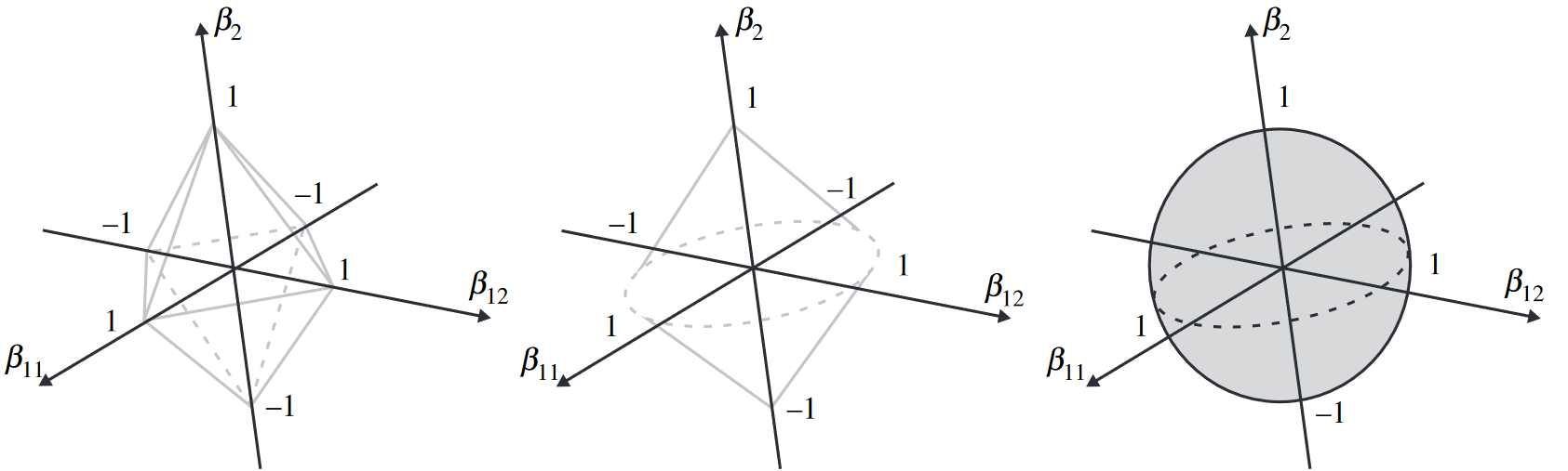
Figure 2: The left image shows the $\ell_{1}$ penalty used in Lasso. The middle image shows the $\ell_{2,1}$ penalty function used in Group Lasso, and the right image shows the $\ell_{2}$ penalty function used in Ridge. $\beta_{11}$ and $\beta_{12}$ are grouped together for Group Lasso. (The image is taken from [228].)

2.3.1 Regularization on BN Parameters

Batch Normalization (BN) layers have been widely used in many modern CNNs to improve model generalization. By normalizing each training mini-batch, the internal covariate shift is addressed. The following equation describes the operations of a BN layer (NS [74]),

$$\hat{\mathbf{z}}=\frac{\mathbf{z}_{\mathrm{in}}-\mu_{\mathcal{B}}}{\sqrt{\sigma_{\mathcal{B}}^{2}+\epsilon}};\quad\mathbf{z}_{\mathrm{out}}=\gamma\hat{\mathbf{z}}+\beta$$ (6)

where $N_{l+1}$-dimension $\mathbf{z}_{\mathrm{in}}$ and $\mathbf{z}_{\mathrm{out}}$ are the inputs and outputs of a BN layer, $\mu_{\mathcal{B}}$ and $\sigma_{\mathcal{B}}$ are the mean and standard deviation over the current mini-batch ${\mathcal{B}}$. $\epsilon$ is a small number to prevent division by zero. $\gamma\in\mathbb{R}^{N_{l+1}}$ and $\beta\in\mathbb{R}^{N_{l+1}}$ are the learnable parameters, indicating scale and shift, respectively. BN parameters are used as gates for filter pruning because the number of learnable parameters is equal to the number of feature maps and filters.

Network Slimming (NS) [74] directly uses the scaling parameter $\gamma$ in BN to control output channels. The channel-level sparsity-induced $\ell_{1}$ regularization is then introduced to jointly train the weights together with the $\gamma$. After training, the corresponding channels that have close-to-zero $\gamma$ are pruned. To optimize the non-smooth $\ell_{1}$ penalty term, a subgradient descent method [229] is used.

Similar to the situation in NS [74], Gated Batch Normalization (GBN) [75] uses $\gamma$ as the channel-wise gate and $\ell_{1}$-norm of $\gamma$ as the regularization term. A Tick-Tock pruning framework is proposed to boost accuracy by iterative pruning. The Tick phase trains the network with little data, and only the gates and final linear layer are allowed to be updated during training for one epoch. Meanwhile, channel importance is computed by the first-order Taylor Expansion for a global filter ranking. The Tock phase then fine-tunes the sparse network with sparsity constraints.

Polarization Regularization (PR) [76] provides a variant $\ell_{1}$-based regularizer to polarize the scaling factors $\gamma$. It contends that in most sparsity regularization methods, such as NS [74], a naive $\ell_{1}$ regularizer converges all scaling factors to zero indiscriminately. A more reasonable approach is to push the scaling factors of unimportant neurons to zero and those of important neurons to a large value. To achieve the polarization effect, another penalty term is added to the naive $\ell_{1}$ term, separating $\gamma$ from their mean as far as possible. Similar to NS [74], subgradients [229] are used on non-differentiable points to solve the non-smooth regularizer.

Rethinking Smaller-Norm-Less-Informative (RSNLI) [77] is developed from the basis of previous methods tending to suffer from the Model Reparameterization problem and the Transform Invariance problem. As there are doubts whether smaller-norm parameters are less informative; Ye et al. propose to train with ISTA [230] to enforce sparsity on $\gamma$. The channel with a $\gamma$ equal to zero is pruned. Then the $\gamma$-$W$ rescaling trick is used on $\gamma$ and weights to quickly start the sparsification process.

Operation-aware Soft Channel Pruning (SCP) [78] considers both BN and ReLU operations. In contrast to NS [74] making decision merely on the channel scaling $\gamma$, Kang et al. also consider shifting parameters $\beta$. Specifically, channels with large negative $\beta$ and large $\gamma$ are considered unimportant since these channels will become zero after ReLU. To consider BN’s large negative mean values, the cumulative distribution function (CDF) of a Gaussian distribution parameterized by $\beta$ and $\gamma$ is used as the indicator function. To optimize $\beta$ and $\gamma$, a sparsity-loss-inducing large CDF value is designed to encourage the network to be more sparse.

EagleEye [79] proposes a three-stage pipeline. First, pruning strategies (i.e., layer-wise pruning ratio) are generated by simple random sampling. Second, sub-networks are generated according to the pruning strategies and $\ell_{1}$-norm of filters. Third, an adaptive-BN-based candidate evaluation module is used to evaluate the performance of the sub-networks. Li et al. contend that outdated BN statistics are unfair to sub-network evaluations, and that BN statistics for each candidate should be re-calculated on a small part of the training dataset [79]. After evaluating sub-networks with the adaptive BN statistics, the best-performing one is selected as the final pruned model.

2.3.2 Regularization on Extra Parameter

Although some studies [77, 75] make special adjustments for networks without BN layers, introducing extra parameters is a more general solution. The extra parameters $\theta$ are trainable and parameterize the gates $g(\theta)$ in determining the pruning results.

To find a sparse structure, Sparse Structure Selection (SSS) [80] attempts to force the output of structures to zero. A scaling factor $\theta$ is introduced after each structure, i.e., neuron, group or residual block. When $\theta$ is lower than a threshold, the corresponding structure is removed. The gate $g(\theta)$ function is:

$$g(\theta)=\begin{cases}0,&\theta<\text{Threshold}\\ 1,&\text{otherwise}\end{cases}.$$ (7)

It adopts a convex relaxation $\ell_{1}$-norm as the sparsity regularization on the extra parameter $\theta$. To update $\theta$, a modified Accelerated Proximal Gradient [231] is used.

Generative Adversarial Learning (GAL) [81] jointly prunes structures and adopts a Generative Adversarial Network (GAN) to achieve label-free learning. Extra scaling factors are introduced after each structure in the generator, forming soft masks. During training, a special regularization term that contains three regularizers is proposed: 1) a $\ell_{2}$ weight decay regularizer on generators, 2) a $\ell_{1}$ sparsity regularizer on the mask, and 3) an adversarial regularization on discriminator. Furthermore, FISTA [230] is used to iteratively update the generator and discriminator, and the mask is updated together with the generator.

Discrete Model Compression (DMC) [82] explicitly introduces discrete (binary) gates after the feature map to precisely reflect the pruned channels’ impact on the loss function. First, it samples subnetworks with stochastic discrete gates:

$$g(\theta)=\begin{cases}1,&\text{w.p. }\theta\\ 0,&\text{w.p. }1-\theta\end{cases}$$ (8)

where w.p. stands for “with probability”. The stochastic nature of the gate ensures that every channel has the chance to be sampled if $\theta\neq 0$, so different subnetworks can be produced. To update the non-differentiable binary gates, a Straight-Through Estimator [232] is adopted.

Similar to PR [76], Gates with Differentiable Polarization (GDP-Guo) [83] aims to polarize gates. Designing a gate with a polarization effect wields the property of smoothed $\ell_{0}$ formulation [233]:

$$g(\theta)=\frac{\theta^{2}}{\theta^{2}+\epsilon}\quad\xrightarrow{\text{has property}}\quad g(\theta)=\begin{cases}\approx 1,&\theta\neq 0\\ =0,&\theta=0\end{cases}$$ (9)

where $\epsilon$ is a small positive value to prevent zero division. This property polarizes $\theta$ to either exactly $0$ or values close to $1$. The gate itself is differentiable. However, the sparsity regularization on $\theta$ involves $\ell_{0}$-norm and renders the objective function non-differentiable. Thus, proximal-SGD [234] is used to update $\theta$.

Convolutional Re-parameterization and Gradient Resetting (ResRep) [84] re-parameterizes a CNN into two parts. The first “remembering part” learns to maintain the model’s performance and will not be pruned. The second “forgetting part” inserts $1\times 1$ CONV layers, or the compactors, after the BN layers. During training, a modified SGD update rule updates the compactors only. Thus, only compactors are allowed to forget (forgetting) while other CONV layers are kept untouched (remembering).

Scientific Control Pruning (SCOP) [85] believes that the importance of a filter may be disturbed by potential factors such as input data. For example, the filter importance ranking may vary if input data is slightly changed for data-dependent methods. To minimize the effect of potential factors, it prunes under scientific control by creating knockoff counterparts [235]. Knockoff features are identical to the real features except for not knowing the true label. Two scaling factors $\theta$ and $\tilde{\theta}$ are then introduced to control the participation of real and knockoff features, respectively. The two parameters are complementary that $\theta+\tilde{\theta}=\mathbf{1}$. If $\theta$ cannot suppress $\tilde{\theta}$, the real features are deemed to have little or no association with the true output. Thus, the filter importance score is defined as $\mathcal{I}=\theta-\tilde{\theta}$, and filters with small importance scores are deemed redundant.

To directly control the model budget, Budget-Aware Regularization (BAR) [86] uses a prior loss and introduces a learnable dropout parameter $\theta$ [236]. The prior loss is the product of two functions. The first function is an approximation of budgets that is differentiable w.r.t. $\theta$. The second function is a variant log-barrier function [237] that employs a sigmoidal schedule. The novel objective function consists of the prior loss, enabling simultaneous training and pruning according to the budget. Knowledge distillation is then used to improve accuracy.

2.3.3 Regularization on Filters

Structured Sparsity Learning (SSL) [91] uses Group Lasso to prune channels. Removing layer $l$’s channel will cause the removal of layer $l$’s filters and layer $l+1$’s input channels. Hence, it adds two separate regularization terms for filter-wise and channel-wise pruning:

$$\sum_{n_{l}=1}^{N_{l+1}}\left\|\mathbf{W}_{n_{l},:,:,:}^{(l)}\right\|_{2},\qquad\sum_{c_{l}=1}^{N_{l}}\left\|\mathbf{W}_{:,c_{l},:,:}^{(l)}\right\|_{2},$$ (10)

where $\mathbf{W}^{(l)}\in\mathbb{R}^{N_{l+1}\times N_{l}\times K_{l}\times K_{l}}$.

Out-In-Channel Sparsity Regularization (OICSR) [92] uses Group Lasso to jointly regularize filters that work cooperatively. The regularization term is:

$$\sum_{i=1}^{N}\left\|\mathbf{W}_{i,:}^{(l)}\oplus\mathbf{W}_{:,i}^{(l+1)}\right\|_{2},$$ (11)

where $\oplus$ denotes concatenation of the out-channel filters $\mathbf{W}^{(l)}_{i,:}\in\mathbb{R}^{N_{l+1}\times(N_{l}K_{l}K_{l})}$ and the in-channel filters $\mathbf{W}^{(l+1)}_{:,i}\in\mathbb{R}^{(N_{l+2}K_{l+1}K_{l+1})\times N_{l+1}}$. It uses the premise that out-channel filters of layer $l$ are interdependent of in-channel filters of layer $l+1$, so these filters should be regularized together.

Only Train Once (OTO) [93] contends that even if all filter weights are zeros, the activation maps will be non-zero because of three parameters: 1) convolution bias, 2) BN mean, and 3) BN variance. Instead of grouping only filters, this method groups all parameters that cause a non-zero activation into a group named the zero-invariant group. Structured sparsity is then introduced to this group by applying the mixed $\ell_{1}/\ell_{2}$-norm. To solve the non-smooth mixed-norm regularization, a stochastic optimization algorithm named Half-Space Stochastic Projected Gradient is used.

Growing Regularization (GREG) [94] exploits regularization under a growing penalty and uses two algorithms. The first algorithm focuses on the pruning schedule and adopts $\ell_{1}$-norm [14] to obtain a mask for pruning. Instead of immediately removing unimportant filters, a growing $\ell_{2}$ penalty is used to gradually drive them to zero. The second algorithm uses a growing regularization to exploit the underlying Hessian information. The authors observe that the weight discrepancy increases as the regularization parameter increases, and weights will naturally separate. If the discrepancy is large enough, even a simple $\ell_{1}$-norm can be an accurate criterion.

2.4 Optimization Tools

Optimization tools are integrated into the pruning process to find or induce structured sparsity in neural networks. For example, Taylor Expansion finds filter importance by approximating the loss function when a specific filter becomes zero. Variational Bayesian methods determine filter importance by exploiting the prior and posterior distributions. SGD-based methods modify the gradient update rule to detect and resolve redundant filters. ADMM-based methods impose structured sparsity constraints and find solutions by using the ADMM optimization algorithm. Bayesian Optimization helps reduce the “curse of dimensionality problem” [238] encountered while learning the optimal sparse structures.

2.4.1 Taylor Expansion

Taylor Expansion [239] expands a function into the Taylor Series, which is an infinite sum of terms. The Taylor Expansion of a function $f(x)$ expands at some point $a$:

$$f(x)=\overbrace{\underbrace{f(a)+\frac{f^{\prime}(a)}{1!}(x-a)}_{\text{first-order approximation}}+\frac{f^{\prime\prime}(a)}{2!}(x-a)^{2}}^{\text{second-order approximation}}+\underbrace{R_{2}(x)}_{\text{remainders}},$$ (12)

where $f^{\prime}(\cdot)$ and $f^{\prime\prime}(\cdot)$ is the first-order derivative and second-order derivative with respect to $x$, respectively.

In structured pruning, Taylor Expansion is used to approximate the change in the loss $\Delta\mathcal{L}$ of pruning structures such as filters or channels. Since pruned weights are set to $0$, the loss function $\mathcal{L}(w)$ of weights $w$ can be evaluated at $a=0$ using Taylor Expansion. By manipulating Eq. 12, we can get:

$$\mathcal{L}(w)-\mathcal{L}(0) =\frac{\mathcal{L}^{\prime}(0)}{1!}(w-0)+\frac{\mathcal{L}^{\prime\prime}(0)}{2!}(w-0)^{2}+R_{2}(w).$$ (13)

Let $\mathcal{L}(w)-\mathcal{L}(0)=\Delta\mathcal{L}$ be the change in the loss of removing some weights, and $w-0=\Delta w$ be the change in the weights. We can get the following equation based on [98],

$$\Delta\mathcal{L}=\frac{\partial\mathcal{L}^{\top}}{\partial w}\Delta w+\frac{1}{2}\Delta w^{\top}\mathbf{H}\Delta w+R_{2}(w)$$ (14)

where $\frac{\partial\mathcal{L}}{\partial w}$ is the first-order gradient of loss function w.r.t. weights, and $\mathbf{H}$ is the Hessian matrix containing second-order derivatives. Compared to regularization-based methods, pruning with Taylor Expansion does not need to wait until the activations are trained sufficiently small [96].

First-order and second-order Taylor expansions have their own characteristics. The second-order expansion contains more information, but it requires calculating the second-degree derivatives that are computationally prohibitive. On the contrary, the first-order expansion can be obtained from backpropagation without requiring additional memory, but this provides less information.

First-order-Taylor: Mol-16 [95] uses the first-order information to estimate the change in the loss of pruning activation maps. The higher-order remainders, including the second-order term, are discarded since they are computationally intractable and are encouraged to be small by the widely-used ReLU activation function. Thus, the absolute change in loss approximated by the first-order term is used as the metric for feature map importance:

$$\left|\frac{1}{M}\sum_{m}\frac{\partial\mathcal{L}}{\partial z_{m}}z_{m}\right|,$$ (15)

where $M$ is the length of a flattened feature map, and $z$ is an activation in a feature map. After determining the feature map importance, the lowest-ranked maps will be pruned.

Compared to Mol-16 [95], which fails with skip connections, Mol-19 [96] proposes a more general method that uses Taylor expansion to approximate the squared change in the final loss. Unlike Mol-16’s [95] use of activations that increase memory consumption, Mol-19 [96] computes the importance $\mathcal{I}$ based on weights:

$$\mathcal{I}_{\mathcal{S}}(\mathbf{W})\triangleq\sum_{s\in\mathcal{S}}\left(\frac{\partial\mathcal{L}}{\partial w_{s}}w_{s}\right)^{2},$$ (16)

where $\mathcal{S}$ is a structural set of parameters such as a convolutional filter, $w_{s}$ is the individual weight of the filter, and $\frac{\partial\mathcal{L}}{\partial w_{s}}$ represents the gradient. The first-order expansion performs significantly faster than the second-order expansion with a slightly higher accuracy drop.

Due to the simplicity and efficiency of computing, the first-order expansion is widely adopted by many methods such as GBN [75] and GDP-Lin [116] which are discussed in other sections.

Second-order-Taylor: In this sub-section, the Hessian matrix $\mathbf{H}$ that contains second-order information from Eq. 14 is exploited. First, pioneering unstructured studies are briefly introduced. Second, the structured pruning methods are addressed.

Pioneering unstructured studies: Most current structured pruning methods that use second-order Taylor expansion are based on two pioneering studies on unstructured pruning: Optimal Brain Damage (OBD) [240] and Optimal Brain Surgeon (OBS) [241]. OBD [240] assumes that $\mathbf{H}$ is diagonal to ease computation. The diagonal $\mathbf{H}$ is then used to compute the parameter importance. However, OBS [241] finds that most of the Hessian matrices $\mathbf{H}$ are strongly non-diagonal. Thus, the full $\mathbf{H}$ is used and the parameter importance is calculated by $\mathbf{H}^{-1}$.

Structured pruning methods: With the success of OBD [240] and OBS [241] in unstructured pruning, the second-order expansion is applied to structured pruning. As deep CNNs have millions of parameters, computing and storing the Hessian $\mathbf{H}$ become challenging [97]. Recent methods aim to approximate the Hessian matrix for structured pruning.

Collaborative Channel Pruning (CCP) [97] approximates the Hessian matrix by only using the first-order derivative of a pre-trained model. The first-order information can be retrieved from backpropagation, and no additional storage is needed. In addition, Peng et al. exploit the effect of removing multiple channels instead of a single channel. The non-diagonal element in $\mathbf{H}$ reflects the interaction between two channels and hence exploits the inter-channel dependency. CCP models the channel selection problem as a constrained 0-1 quadratic optimization problem to evaluate the joint impact of pruned and unpruned channels.

Eigen Damage (ED) [98] introduces a baseline method that is the naive structured extension of OBD [240] and OBS [241]. Two algorithms are then applied to improve the baseline method. The baseline method sums up the individual change in parameters over a filter, raising the granularity to the filter level. However, computing and storing the Hessian $\mathbf{H}$ is intractable. Wang et al. propose the use of the first algorithm [98] that applies K-FAC [242] approximation to decompose filters. As the naive extensions and the first algorithm both fail at capturing the correlation between filters, a second algorithm which decorrelates the weights before pruning is applied. This second algorithm adopts K-FAC [242] and projects weight space to a Kronecker-Factored eigenspace (KFE) [243] where there is little correlation.

Group Fisher Pruning (GFP) [99] addresses the difficulties faced by other pruning methods when channels from multiple layers are coupled and require simultaneous pruning. First, a layer grouping algorithm is used to automatically identify coupled channels. Second, the Hessian information is used as a unified importance criterion of a single channel and coupled channels. With the help of the Fisher information, the Hessian matrix is transformed into the square of first-order derivatives.

2.4.2 Variational Bayesian

Bayesian inference [244] is a method to infer the posterior probability distribution $p(\theta|x)$ with the known prior probability distribution $p(\theta)$ of parameters $\theta$ and the observed data $x$. The formula to compute the posterior distribution over $\theta$ is given:

$$\overbrace{p(\theta|x)}^{\text{Posterior}}=\frac{\overbrace{p(x|\theta)}^{\text{Likelihood}}\cdot\overbrace{p(\theta)}^{\text{Piror}}}{\underbrace{p(x)}_{\text{Evidence}}},\text{where }p(x)=\int p(x|\theta)p(\theta)d\theta.$$ (17)

However, computing the evidence often requires computationally intractable integrals when large amounts of data are involved. Variational Bayesian (VB) methods [245] are used to approximate the posterior distribution $p(\theta|x)$ by a variational distribution $q(\theta)$. Specifically, $q(\theta)$ is optimized by minimizing the Kullback–Leibler (KL) divergence which measures the “similarity” between $q(\theta)$ and $p(\theta|x)$. Since the computation of KL-divergence involves the intractable posterior distributed $p(\theta|x)$, the optimization problem is solved by equivalently converting it to maximize the Evidence Lower BOund (ELBO).

Variational Pruning (VP) [102] is based on channel importance being indicated by random variables, as pruning by deterministic channel importance is inherently improper and unstable. Thus, BN’s parameter $\gamma$ is used to indicate the channel saliency and model $\gamma$ by Gaussian distribution $\mathcal{N}\left(\mu,\sigma\right)$. To introduce sparsity, VP utilizes the centrality property of the Gaussian distribution $\mathcal{N}$ and samples $\gamma$ from $\mathcal{N}\left(\mu=0,\sigma\right)$ as the sparse prior distribution. After optimizing ELBO, distributions of $\gamma$ with close-to-zero mean and small variance are considered safe for pruning, since such distributions are less likely to have salient parameters.

To find redundant channels, Recursive Bayesian Pruning (RBP) [103] targets the posterior of redundancy, which assumes an inter-layer dependency among channels. First, each input channel is scaled by a dropout noise $\theta$ [236, 105] with a dropout rate $r$. Second, the dropout noises are then modeled across layers as a Markov chain to exploit the inter-layer dependency among channels. To get the posterior of redundancy, a sparsity-inducing Dirac-like prior is chosen. In addition, RBP [103] adopts the reparameterization trick [236] to scale the noise $\theta$ on the corresponding channels to consider data fitness. As a result, the dropout rate $r$ can be updated along with weights in a gradient-based manner. Pruning is conducted by setting the corresponding channels to zero when $r$ is greater than a threshold.

A few other studies also use the Bayesian point of view. VIBNet [104] uses a variational information bottleneck, which is the informational theoretical measure of redundancy between adjacent layers. Louizos et al. [105] utilize the horseshoe prior to efficiently approximate channel redundancy. Neklyudov et al. [106] use a log-normal prior, resulting in a tractable and interpretable log-normal posterior.

2.4.3 Others

SGD-based: Instead of zeroing out filters, Centripetal SGD (C-SGD) [107] makes redundant filters identical and merges identical filters into one filter. Regularized Modernized Dual Averaging (RMDA) [108] adds momentum to the RDA algorithm [246] and ensures that the trained model has the same structure as the original model. To prune the model, RMDA adopts Group Lasso to promote structured sparsity.

ADMM-based: Alternating Direction Method of Multipliers (ADMM) [247] is an optimization algorithm used to decompose the initial problem into two smaller, more tractable subproblems. StructADMM [111] studies the solution of different types of structured sparsity such as filter-wise and shape-wise. Zhang et al. use a progressive and multi-step ADMM framework: at each step, it uses ADMM to prune and masks out zero weights, leaving the remaining weights as the optimization space for the next step.

Bayesian Optimization: Bayesian optimization (BO) [248] is a sequential design strategy for the global optimization of black-box functions that does not assume any functional forms. When pruning a model that involves an extremely large design space, the curse of dimensionality problem occurs [249]. Rollback [113] adopts the RL-style automatic channel pruning [130] and uses BO to determine the optimal pruning policy.

Soft Threshold: Soft threshold  [250] is a de-noising operator in the area of digital signal processing. Soft Threshold Reparameterization (STR) [114] adopts this operator to learn a non-uniform sparsity budget which is optimized per layer.

2.5 Dynamic Pruning

Structured pruning can be conducted in a dynamic manner during both training and inference. Dynamic during training aims to preserve the model’s representative capacity by maintaining a dynamic pruning mask during training. It is also called soft pruning to ensure that improper pruning decisions can be recovered later. On the other hand, hard pruning permanently removes weights with a fixed mask. Dynamic during inference indicates the networks are pruned dynamically according to different input samples. For instance, a simple image that contains clear targets requires less model capacity compared to a complex image [108]. Hence, dynamic inference provides better resource-accuracy trade-offs.

2.5.1 Dynamic during Training

Weight-level dynamic: The concept of training-time dynamic pruning was first introduced in Dynamic Network Surgery (DNS) [251], an unstructured pruning approach. To clarify the difference between other approaches, its formulation is:

$$\mathbf{W}^{l}_{i,j}\leftarrow\mathbf{W}^{l}_{i,j}-\eta\frac{\partial\mathcal{L}(\mathbf{W}^{l}\odot\mathbf{T}^{l})}{\partial(\mathbf{W}^{l}_{i,j}\mathbf{T}^{l}_{i,j})},$$ (18)

where $\eta$ is the learning rate and $\odot$ denotes the Hadamard Product operator. $\mathbf{W}^{l}$ is the weight matrix in the $l$-th layer with all weights of kernels unfolded and concatenated together. $\mathbf{T}^{l}$ is the binary mask that has the same shape as the weight matrix, indicating the importance of the weights. $\mathcal{L(\cdot)}$ is the loss function. $\mathbf{W}_{i,j}^{l}$ and $\mathbf{T}_{i,j}^{l}$ indicate a single element in $\mathbf{W}^{l}$ and $\mathbf{T}^{l}$. $\mathbf{W}$ and $\mathbf{T}$ are updated alternatively. All the weights are updated, so wrongly pruned parameters have a chance to regrow.

Filter-level dynamic: Soft filter Pruning (SFP) [115] adopts the idea of dynamic pruning in a structured way. Its use is based on the premise that hard pruning that uses a fixed mask throughout the training will reduce the optimization space. Therefore, it dynamically generates the masks based on the $\ell_{2}$-norm of filters at every epoch. Soft pruning means setting the values of filters to zero instead of removing filters. Previously soft-pruned filters are allowed to be updated at the next epoch, during which masks will be reformed based on new weights. The update rule is:

$$\mathbf{W}^{l}\leftarrow\mathbf{W}^{l}-\eta\frac{\partial\mathcal{L}\left(\mathbf{W}^{l}\odot\mathbf{m}^{l}\right)}{\partial\left(\mathbf{W}^{l}\odot\mathbf{m}^{l}\right)},$$ (19)

where $\mathbf{W}^{l}\in\mathbb{R}^{N_{l+1}\times N_{l}KK}\text{~{}and~{}}\mathbf{m}^{l}\in\mathbb{R}^{N_{l+1}}$.

Globally Dynamic Pruning (GDP-Lin) [116] also maintains a binary dynamic mask during training based on the filter importance. GDP-Lin adopts the first-order Taylor expansion to approximate the global discriminative power of each filter. In addition, the authors argue that frequently changing masks cannot effectively guide the pruning. Hence, masks are updated every $e$ iteration, where $e$ is set as a decreasing value to accelerate the convergence.

In addition to maintaining a sparse dynamic mask, Dynamic Pruning with Feedback (DPF) [117] simultaneously maintains a dense model. The premise behind its use is that a sparse model can be considered a dense model with compression error. The error can be used as feedback to ensure the correct direction in the gradient updates. For this goal, gradients computed from the sparse model are used to update the dense model. The advantage of applying gradients on a dense model is that it helps weights to recover from errors.

CHannel EXploration (CHEX) [118] uses two processes to dynamically adjust filter importance. The first process is the channel pruning process with Column Subset Selection criterion [252]. The second process is the regrowing process, which is based on orthogonal projection [253] to avoid regrowing redundant channels and to explore channel diversity. Regrowing channels are restored to the most recently used (MRU) parameters rather than zeros. To better preserve model accuracy, the remaining channels are re-distributed dynamically among all the layers.

Dynamic Sparse Graph (DSG) [119] activates a small number of critical neurons with the constructed sparse graph at every iteration dynamically. DSG is developed from the argument that direct computation according to output activations is very costly for finding critical neurons. The dimension reduction search is formulated to forecast the activation output by computing input and filters in a lower dimension. Furthermore, to prevent BN layers from damaging sparsity, Liu et al. introduce the double-mask selection that uses the same selection mask before and after BN layers [119].

Other methods, such as SCP [78] and DMC [82], also maintain the mask dynamically. These are discussed in Section 2.3.

2.5.2 Dynamic during Inference

Runtime Neural Pruning (RNP) [123] is based on the premise that the static model fails to exploit the different properties of input images by using the same weights for both easily recognized and complex pattern images. It uses a framework with CNN as the backbone and RNN as a decision network. The network pruning is modeled as a Markov decision process, and models are trained by reinforcement learning (RL). The RL agent evaluates filter importance and performs channel-wise pruning according to the relative difficulty of samples for a task. Thus, when the image is easier for the task, a sparser network is generated.

Feature Boosting and Suppression (FBS) [124] predicts output channel importance based on inputs by introducing a tiny and differentiable auxiliary network. In the auxiliary network, a 2D global average pooling is used to subsample the activation channels in the previous layer to scalars. The advantage of this is that it reduces the computational overhead in the auxiliary network. A salient predictor then uses the subsampled scalars to generate the predicted saliency scores through a fully connected layer followed by an activation function. The top-$k$ salient channels are finally involved in the inference-time calculation.

Deep Reinforcement Learning pruning (DRLP) [126] learns both the runtime (dynamic) and the static importance of channels. The runtime importance measures the importance of channels specific to an input. In contrast, the static importance measures the channel importance for the whole dataset. Like RNP [123], DRLP uses reinforcement learning (RL). The RL framework contains two parts: one static and one runtime. Each part contains an importance predictor and an agent, providing static/runtime importance and layer-wise pruning ratio, respectively. In addition, a trade-off pruner generates a unified pruning decision based on the outputs from the two parts.

Dynamic Dual Gating (DDG) [127] uses two separate gating modules (spatial and channel gating) to determine inference-time importance according to inputs. The spatial module consists of an adaptive average pooling followed by a 3x3 CONV layer to extract informative spatial features. By having a spatial mask, only informative features are allowed to pass to the next layer. The channel gating module works in a manner similar to existing methods such as FBS [124] by using global average pooling followed by the application of FC layers. To enable gradient flow, the Gumbel-Softmax reparameterization [254] is used for both spatial and channel gating modules.

Fire Together Wire Together (FTWT) [128] models the dynamic pruning task as a self-supervised binary classification problem. The proposed framework uses 1) a prediction head to generate learnable binary masks and 2) a ground truth mask to guide the learning after each convolutional layer. The prediction head consists of a global max pooling layer, a 1x1 CONV layer, and a softmax layer. Then, the outputs from the prediction head are rounded to generate a binary mask. To achieve self-supervised learning, ground truth binary masks are needed; by ranking the norm of input activations, ground truth pruning decisions are made to guide the learning.

At the same time, Contrastive Dual Gating (CDG) [129] implements another self-supervised dynamic pruning framework by using contrastive learning [255]. Contrastive learning trains a model from the latent contrastiveness of high-level features of two contrastive branches. Therefore, a similarity-based contrastive loss [256] is used for gradient-based learning without the labeled data. Empirical studies show that pruning decisions cannot be transferred between contrastive branches. Thus, dual gating is introduced, and the two branches have distinct pruning masks. CDG [129] uses a framework similar to that of CGNet [257] for each contrastive branch. Like DDG [127], a 3x3 CONV layer is used to extract spatial features for unpruned features.

2.6 NAS-Based Pruning

Given that it is cumbersome to manually determine pruning-related hyperparameters such as the layer-wise pruning ratio, NAS-based Pruning has been proposed to automatically find pruned structures. Based on the survey of Neural Architecture Search (NAS) [26], we categorize NAS for pruning into three methods. NAS can be modeled as:

1. reinforcement learning (RL) problems, in which RL agents find sparse subnetworks by searching over the action space such as pruning ratios.

2. gradient-based methods that modify the gradient update rule to make optimization problems with sparsity constraints differentiable to weights.

3. evolutionary methods that adopt evolutionary algorithms to explore and search the sparse subnetworks.

2.6.1 Reinforcement Learning-Based

AutoML for Model Compression (AMC) [130] uses RL to automatically select the appropriate layer-wise pruning ratio without manual sensitivity analysis. To search over a continuous action space, the deep deterministic policy gradient (DDPG) algorithm [258] is adopted. The actor receives 11 layer-dependent states such as FLOPS and outputs a continuous action about the pruning ratio. For accuracy-guaranteed pruning, the reward for the DDPG agent is modified from Eq. 20 to Eq. 21:

$$R_{\mathrm{err}}=-Error$$ (20)

$$R_{\mathrm{FLOPs}}=-Error\cdot\log(\mathrm{FLOPs})$$ (21)

$$R_{\mathrm{Param}}=-Error\cdot\log(\#\mathrm{Param})$$

Automatic Graph encoder-decoder Model Compression (AGMC) [131] adopts the premise that AMC [130] still requires manual selection of the fixed 11 states fed into the RL agent. In addition, the fixed environment states ignore the rich information within the computational graphs. Hence, the DNNs are modeled as computational graphs and fed into a GCN-based graph encoder-decoder [259] to automatically learn the RL agent’s input states. In contrast to AMC [130], AGMC rescales the pruning ratios to compensate for any unmet sparsity constraint rather than applying the FLOPs into the reward function (Eq. 21).

DECORE [132] adopts multi-agent learning. The presence of multiple agents comes from assigning dedicated agents to all channels in a layer, with each agent only learning one parameter representing a binary decision. In contrast to AMC [130] and AGMC [131], DECORE models the state of the channel itself. To learn the action parameters, a higher reward is given when the accuracy retention task and compression task are both well-completed:

$$\begin{gathered}R^{l}_{\mathrm{comp.}}=\sum_{j=1}^{N_{l+1}}1-a^{l}_{j},\quad R_{\mathrm{acc}}=\left\{\begin{array}[]{cc}1&\text{ if }\hat{y}=y\\ -\lambda&\text{ else }\end{array}\right.\\[2.0pt] R^{l}=R^{l}_{\mathrm{comp.}}*R_{\mathrm{acc}}\end{gathered}$$ (22)

where $N_{l+1}$ represents the output channel size of layer $l$, $a^{l}$ is the action vector of layer $l$, $y$ and $\hat{y}$ are the true label and predicted label, and $-\lambda$ is a large penalty for a wrong prediction. The reward function does not consider the FLOPs; instead, the reward for the compression task simply takes into account the number of channels remaining.

GNN-RL [133] first models the DNN into a multi-stage graph neural network (GNN) to learn the global topology. The generated hierarchical computational graph is then used as the environmental state of the agent. In contrast to AMC [130] and AGMC [131] that both use DDPG, this method uses the Proximal Policy Optimization (PPO) algorithm [260] as the policy since PPO gives a much better experiment result. In addition, due to the specially designed graph environment, the reward for the RL system does not need to contain sparsity constraints. Accuracy is the only metric for the reward described by Eq. 20.

2.6.2 Gradient-Based

To search for the layer-wise sparsity, Differentiable Markov Channel Pruning (DMCP) [136] models channel pruning as a Markov process. Here, the state means retaining the channel during pruning, and transitions between states represent the pruning process. DMCP parameterizes both the transition and budget loss by learnable architecture parameters. The final loss is thus differentiable w.r.t. architecture parameters. Two stages are used to finish pruning in a gradient-based manner. The first stage updates weights of unpruned networks with a variant sandwich rule [261]. The second stage updates the architecture parameters.

Differentiable Sparsity Allocation (DSA) [137] optimizes the sparsity allocation in continuous space using a gradient-based method that is more effective than a discrete search. The validation loss is adopted as a differentiable surrogate to render the evaluation of validation accuracy differentiable. Next, a probabilistic differentiable pruning process is used as a replacement for the non-differentiable hard pruning process. Finally, sparsity allocation is obtained under a budget constraint. An ADMM-inspired optimization method [247] is used to solve the constrained non-convex optimization problem.

Differentiable Hyper Pruning (DHP) [138] uses hypernetworks that generate weights for backbone networks. The designed hypernetwork consists of three layers. 1) The latent layer first takes two learnable latent vectors $\{\mathbf{z}^{l}\text{ and }\mathbf{z}^{l-1},\mathbf{z}^{l}\in\mathbb{R}^{N_{l+1}}\}$ and forms the latent matrix. Then 2) the embedding layer projects the latent matrix to embedding space, forming embedding vectors. Finally, 3) the explicit layer takes embedding vectors and outputs weights that can be explicitly used as weights for CONV layers. Pruning is done by regularizing the latent vectors with $\ell_{1}$ sparsity regularization, and proximal gradient algorithms [237] are used to update the latent vectors. This method is approximately differentiable since the proximal operation step has a closed-form solution.

Learning Filter Pruning Criteria (LFPC) [140] searches for layer-wise pruning criteria instead of pruning ratios. The basis for its use is that filters have differing distributions for extracting coarse and fine-level features. This makes using the same pruning criterion for all layers inappropriate. To explore the criteria space, criteria parameters are introduced to guide the choice of criteria. To enable gradient flow, this method uses the Gumbel-Softmax reparameterization [254] to make the loss differentiable to criteria parameters.

Transformable Architecture Search (TAS) [141] searches the width and depth of a network. Two learnable parameters, $\alpha$ and $\beta$, are introduced to indicate the distribution of the possible number of channels and layers, respectively. Subnetworks can be sampled based on $\alpha$ and $\beta$. Applying the Gumbel-Softmax reparameterization [254] makes the sampling process differentiable. The search objectives are minimizing the validation loss while encouraging smaller computational costs and penalizing the unmet resources budget. Knowledge Distillation is further used to boost the performance of the pruned networks.

Exploration and Estimation (EE) [142] achieves channel pruning in a two-step gradient-based manner. The first step is exploration of subnetworks to allow larger search space with a fast sampling technique (Stochastic Gradient Hamiltonian Monte Carlo [262]). To bring sparsity, this method applies a FLOPs-aware prior distribution to the exploration process. The second step, estimation, is used to guide the generation of high-quality subnetworks.

2.6.3 Evolutionary-Based

MetaPruning [148] aims to find the optimal layer-wise channel number with a two-stage framework. The first stage trains a meta network named PruningNet to generate various structures. PruningNet takes randomly sampled encoding vectors representing structures and learns in an end-to-end manner. In the second stage, an evolutionary search algorithm is deployed to search for the optimal structures under constraints. No fine-tuning is needed at search time since PruningNet predicts the weights for all the pruned nets.

In contrast to MetaPruning [148], ABCPruner [149] looks for the optimal layer-wise channel number with a one-stage approach and requires no extra supporting network. In addition, it drastically reduces the combinations of pruned structures by limiting the preserved channels to a given space. To search for the optimal pruned structures, an evolutionary algorithm based on the Artificial Bee Colony algorithm (ABC) [263] is applied.

Instead of using evolutionary algorithms (EA) on the entire network, Cooperative CoEvolution algorithm for Pruning (CCEP) [150] uses cooperative coevolution [264] that groups the network by layer and applies EA on each layer. By decomposing the networks into multiple groups, the search space is drastically decreased. The overall framework uses an iterative prune-and-fine-tune strategy. In each iteration, multiple individual candidates (parents) are generated by randomly pruning filters. Offsprings are generated by conducting bit-wise mutations on parents, where each bit represents the presence of a filter. Individuals are then evaluated with accuracy and FLOPs, and only top-$k$ are retained for the next iteration.

2.7 Extensions

Structured pruning can be extended with the Lottery Ticket Hypothesis, with orthogonal network compression techniques and with different granularity of structured sparsity.

2.7.1 Lottery Ticket Hypothesis

The Lottery Ticket Hypothesis (LTH) [265] claims that “dense, randomly-initialized, feed-forward networks contain subnetworks (winning tickets) that — when trained in isolation — reach test accuracy comparable to the original network in a similar number of iterations.” Weight rewinding is often used in LTH-based papers. In the study by Frankle & Carbin [265], the weights and the learning rate schedule are rewound to the values at epoch $k=0$, in order to find the sparse subnetworks at initialization. Frankle et al. [266] propose to rewind the weights and learning rate schedule to $k>0$ epoch to deal with SGD randomness (noise). Different means of achieving unstructured LTH have been proposed: SNIP [267] preserves the training loss; GraSP [268] preserves the gradient flow; Neural Tangent Kernel (NTK) [269] captures the training dynamics; GF [270] prunes weights that cause the least change to the gradient flow.

Renda et al. [271] propose to rewind the learning rate schedule but not the weight value (learning rate rewinding). Experiments show that rewinding techniques consistently outperform fine-tuning, in which learning rate rewinding outperforms or matches weight rewinding in all scenarios.

Rethinking the Value of Network Pruning (RVNP) [152] re-evaluates the value of network pruning. The argument is that traditional fine-tuning techniques work no better than pruning from scratch. Extending LTH in a structured pruning setting for large-scale datasets fails to yield the lottery ticket.

Early Bird (EB) [153] proposes to find the winning ticket in the early stages of training, rather than fully training the dense network. To find the EB ticket, the mask for the filters is computed based on the Hamming distance between two subnetworks pruned from the same model.

Prospect Pruning (ProsPr) [154] argues that the trainability of the pruned networks should be considered. Trainability exists as the model is going to be trained after pruning. Thus, meta-gradients (gradient-of-gradients) have been proposed as a measure of trainability. Instead of estimating the changes in the loss at initialization, the effect of pruning on the loss over several steps of gradient descent at the beginning of training is estimated in ProsPr.

Early Compression via Gradient Flow Preservation (EarlyCroP) [155] achieves early pruning by solving three key problems. The problem 1) why to prune is solved by extending a GF-based pruning criterion [270] to structured pruning. 2) How to prune is solved by preserving the training dynamics using a connection between the gradient flow and NTK [269]. Lastly, 3) when to prune is solved by finding the lazy kernel regime, which is the phase where pruning has little effect on the training dynamics.

Pruning-aware Training (PaT) [156] tries to resolve the problem of when early pruning should begin? PaT is based on the premise that sub-networks having the same number of remaining neurons can have very different architectures. To determine when the architectures are stable, a novel metric called the early pruning indicator (EPI) that computes the structure similarity of two subnetworks has been proposed.

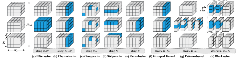
Figure 3: Explain different pruning granularities in three basic dimensions: the output dimension $N_{l+1}$, the input dimension $N_{l}$, and the kernel dimension $K^{2}$. “Along” means the same pruning decision made to all weights at the same position in this dimension. In contrast, “diverse” indicates that pruning results are different in this dimension. (a) Filter-wise and (b) Channel-wise represent well-known structured pruning. Remaining (c) - (h) are special granularities. (c) Group-wise pruning groups weights along the output dimension $N_{l+1}$. (d) Stripe-wise pruning groups weights along the input dimension $N_{l}$. (e) Kernel-wise pruning groups weights along the kernel dimension $K^{2}$. (f) Grouped kernel pruning groups kernels across several different filters in $N_{l+1}$ dimension. (g) Pattern-based pruning utilizes pre-defined patterns to group weights in $N_{l}$ dimension. (h) Block-wise pruning groups kernels with the same pattern in both $N_{l+1}$ and $N_{l}$ dimensions.

2.7.2 Joint Compression

Some prevailing techniques, i.e., architecture search, decomposition and quantization, are orthogonal to pruning methods for neural network compression. Applying these techniques in sequence may seem like a natural extension but can lead to sub-optimal solutions due to different optimization objectives [165]. Therefore, researchers have proposed to apply these techniques jointly.

Pruning and NAS: NPAS [161] develops a framework of joint network pruning and architecture search. This method is compiler-aware and replaces computational activation functions (such as the sigmoid function) with compiler-friendly ones.

Pruning and Quantization: DJPQ [162] jointly performs structured pruning and mixed-bit precision quantization in a gradient-based manner. This structured pruning is based on the variational information bottleneck [104], and mixed-bit precision quantization is extended to power-of-two bit-restricted quantization. Bayesian Bits (BB) [163] unifies the view of mixed precision quantization and pruning, and introduces mixed precision gates on filters for structured pruning. IODF [164] utilizes integer-only arithmetic based on 8-bit quantization and has learnable binary gates to eliminate redundant filters during inference.

Pruning, NAS, and Quantization: APQ [165] performs these tasks jointly. A once-for-all network [272] supporting a large search space for channel number is trained. Next, a quantization-aware accuracy predictor is designed to evaluate the accuracy of the selected structure with mixed-precision quantization [273]. This is followed by the use of an evolutionary-based architecture search [274] to find the best-accuracy model under latency or energy constraints.

Pruning and Decomposition: Some studies have exploited structured pruning and low-rank decomposition within a unified framework. The authors of Hinge [166] contend that pruning techniques cannot deal with the last CONV layer in a residual block that low-rank decomposition is able to. The two techniques are hinged by introducing sparsity-inducing matrices after filters. Imposing group sparsity on the columns and rows of sparsity-inducing matrices achieves filter pruning and decomposition, respectively. Collaborative Compression (CC) [167] simultaneously learns the model sparsity and low-rankness to achieve channel pruning and tensor decomposition jointly.

2.7.3 Special Granularity

Apart from unstructured pruning at the weight level and structured pruning at the filter level, there are also pruning methods at other granularities. To categorize these methods, we define three basic dimensions: output dimension $N_{l+1}$, input dimension $N_{l}$, and kernel dimension $K^{2}$. Filter pruning can be viewed as pruning along dimension $N_{l}\times K^{2}$, and channel pruning is along dimension $N_{l+1}\times K^{2}$. They are similar since pruning filters in the $l$-th layer will remove the corresponding channels in the $l+1$-th layer. More different pruning granularities are shown in Fig. 3.

Group along basic dimensions: GBD [170] and SSL [91] introduce group-wise pruning (Fig. 3c) which prunes weights located at the same position among all filters in a layer, that is, along the output dimension $N_{l+1}$. SWP [171] prunes filters in a stripe-wise (Fig. 3d) manner along input dimension $N_{l}$. Compared to group-wise pruning, stripe-wise pruning maintains filter independence, for there is no pattern across filters. PCONV [172] uses kernel-wise pruning (Fig. 3e) to prune weights along kernel dimension $K^{2}$.

Diverse in basic dimensions: Some researchers find making the same pruning decision along basic dimensions may not be optimal, and they propose to look into the basic dimensions. GKP-TMI [173] uses grouped kernel pruning (Fig. 3f). On top of kernel-wise pruning, this method groups different filters and makes diverse pruning decisions in the output dimension $N_{l+1}$. The remaining kernels are re-permuted to output a densely structured pruned network that benefits from parallel computing. 1xN [174] (Fig. 3f) uses a 1xN pruning pattern which treats $N$ output kernels sharing the same input channel index as the basic pruning granularity. PCONV [172] uses pattern-based pruning (Fig. 3g) by looking into the kernels and making different pruning decisions in the kernel dimension $K^{2}$. Block-wise pruning [161] (Fig. 3h) generalizes pattern-based pruning [172] to share a same pattern for a kernel group, where kernels are grouped in both the output dimension $N_{l+1}$ and the input dimension $N_{l}$. Other possible granularities. There are some more possible structured granularities, such as grouped stripe (extension of Fig. 3d) and grouped pattern (extension of Fig. 3g). Multi-granularity [179] also deserves investigation in structure pruning.

Layer-level: Besides breaking down filters into smaller granularities, Shallowing Deep Networks (SDN) [175] uses layer-wise pruning to prune entire layers. Specifically, SDN places a linear classifier probe [275] after each layer to evaluate the effectiveness of the layer. The network is retrained with the knowledge distillation technique after pruning unimportant layers.

3 Future Directions

3.1 Pruning Topics

Every subsection in Section 2 has the potential for further development in the future. Besides, structured pruning will continue to borrow ideas from unstructured pruning. In this section, we will discuss some promising topics directly related to pruning.

Pruning theory: Apart from utilizing optimization tools for pruning in Section 2.4, some works view pruning from the perspective of synaptic flow [180], signal propagation [181], and graph theory [182]. Besides, the pruning process can be guided by leveraging the interpretations of a model [183], the loss landscape [110], generalization-stability trade-off [184] and entropy of a model [185]. Moreover, the theory behind LTH is investigated with Logarithmic Pruning [186]. In addition, different training methods [187, 188, 189] can be combined with pruning. The above directions have the potential in structure pruning.

Pruning mechanism: Researchers have new views on the prevailing three-stage training-pruning-retraining mechanism. First, the Lottery Ticket Hypothesis, which is proposed on unstructured pruning, is expected to extend on structured pruning. Second, single-shot pruning [190, 191] prunes only once to get the pruned models. Structured pruning can potentially benefit from this mechanism. Third, AC/DC training [192] is able to co-training the dense and sparse models. Therefore, handling multiple models during pruning and training is another promising direction for structured pruning.

Pruning Rate: Structured pruning can also extend the current weight pruning strategies on researching the layer-wise pruning ratios [144, 193, 194].

Pruning Domain: Utilizing representation in the frequency domain [195, 65] to guide pruning is another interesting direction.

3.2 Pruning for Specific Tasks

Pruning techniques can be applied to other tasks to achieve high computational efficiency. Here are some straightforward examples: super-resolution [203], personal re-id [204, 276], medical imaging diagnostic [205], face attribute classification [206] and ensemble learning [207, 208]. Apart from the tasks mentioned above, some emerging directions are still in the early stages but are promising in the future.

Pruning for Federated Learning: Federated learning [277] aims to solve the problem of training a model without transferring data to a central location. Pruning [196, 197] helps alleviate communication costs required between devices and servers. Zhang et al. [196] contend that the non-Independent and Identically Distributed (non-IID) degree for each device and server is different, so it proposes to compute the different pruning ratio from each device and an aggregated expected pruning ratio for the server.

Pruning for Continual Learning: Continual Learning tackles the problem of catastrophic forgetting [198]. Some pioneering works [199, 200, 201] use the pruned filters of the sparsified network to train a new task, so the training process does not cause deterioration to the performance of previous tasks.

Limited Dataset: Dataset compression and pruning [278] are emerging. The idea is to utilize part of the images from the training dataset to train the network. Structured pruning [202] has lots of topics to investigate along with this new trend.

3.3 Pruning Specific Networks

Besides the prevailing CNNs, pruning is beneficial to other type of neural networks such as MLPs [217], rectifier neural networks [218], spiking neural networks [219, 220], and Generative adversarial network (GAN) [209, 210, 212, 211].

Pruning CNN-Based Transformers: There has been a growing trend to incorporate the architectural design of CNNs into Transformer models [16, 17, 18, 19, 20]. Therefore, adopting these structured pruning techniques to compress these novel architecture designs is meaningful [15, 213].

Pruning Transformer-Based Architecture: The attention mechanism of Transformer architecture fundamentally operates using fully connected layers, which can be perceived as a unique manifestation of convolutional layers when the kernel size is set to 1 [279]. In recent years, foundation models [214] such as GPT-3 [215] and generalist agents such as Gato [216] are the possible way to Artificial general intelligence (AGI). The efficiency of attention components of these huge models can benefit from the research of structured pruning.

3.4 Pruning Targets

During past years, the target of pruning has shifted from reducing the number of parameters in unstructured pruning to minimizing the FLOPs in structured pruning. Recently, the target of pruning has been evolving to meet the practical demands of real-world scenarios.

Hardware: Incorporating pruning into the hardware process is an emerging trend. Hardware compiler-aware pruning [221] conducts pruning based on the structural information of subgraphs constructed during compiler tuning.

Energy: As the deployment of AI models expands, the rising energy consumption of AI models needs greater attention. Considering energy during pruning should be investigated. Energy-aware pruning [222] greedily prunes the layer that consumes the most energy, for minimizing the MACs may not necessarily reduce the most energy consumption.

Robustness: The robustness of a network describes how easily a network is fooled to make a wrong prediction under attacks [223]. Considering the robustness and computational cost of models together during the model design process is a new trend. Researchers find that sparsity brought by pruning can improve the adversarial robustness [280]. Linearity Grafting (Grafting) [224] operates on the premise that network robustness favors linear functions and proposes the linearity grafting method. ANP-VS [225] identifies the latent features with high vulnerability and proposes a Bayesian framework to prune these features by minimizing adversarial loss and feature-level vulnerability.

Yang He received the B.S. degree and M.Sc. from the University of Science and Technology of China, Hefei, China, in 2014 and 2017, respectively. He received his Ph.D. degree from the University of Technology Sydney in 2022. He currently is a scientist with the Centre for Frontier AI Research (CFAR), Agency for Science, Technology and Research (A*STAR), Singapore, and also with the Institute of High Performance Computing (IHPC), Agency for Science, Technology and Research (A*STAR), Singapore. His research interests include deep learning, computer vision, and filter pruning.

Lingao Xiao is an intern student with the Centre for Frontier AI Research (CFAR), Agency for Science Technology and Research (A*STAR), Singapore, and also with the Institute of High Performance Computing (IHPC), Agency for Science, Technology and Research (A*STAR), Singapore. He is pursuing his bachelor’s degree in computer engineering at Nanyang Technological University, Singapore. His research interests include network compression and filter pruning.

See pages - of supp.pdf

References

- [1] S. Han, H. Mao, and W. J. Dally, “Deep compression: Compressing deep neural networks with pruning, trained quantization and huffman coding,” in Proc. Int. Conf. Learn. Represent., 2016.
- [2] J. Redmon, S. Divvala, R. Girshick, and A. Farhadi, “You only look once: Unified, real-time object detection,” in Proc. IEEE Conf. Comput. Vis. Pattern Recog., 2016, pp. 779–788.
- [3] S. Minaee, Y. Boykov, F. Porikli, A. Plaza, N. Kehtarnavaz, and D. Terzopoulos, “Image segmentation using deep learning: A survey,” IEEE Trans. Pattern Anal. Mach. Intell., vol. 44, no. 7, pp. 3523–3542, 2022.
- [4] Y. Yang, Y. Zhuang, and Y. Pan, “Multiple knowledge representation for big data artificial intelligence: framework, applications, and case studies,” Frontiers of Information Technology & Electronic Engineering, vol. 22, no. 12, pp. 1551–1558, 2021.
- [5] A. Krizhevsky, I. Sutskever, and G. E. Hinton, “Imagenet classification with deep convolutional neural networks,” in Proc. Adv. Neural Inform. Process. Syst., 2012.
- [6] K. Simonyan and A. Zisserman, “Very deep convolutional networks for large-scale image recognition,” in Proc. Int. Conf. Learn. Represent., 2015.
- [7] C. Szegedy, W. Liu, Y. Jia, P. Sermanet, S. Reed, D. Anguelov, D. Erhan, V. Vanhoucke, and A. Rabinovich, “Going deeper with convolutions,” in Proc. IEEE Conf. Comput. Vis. Pattern Recog., 2015, pp. 1–9.
- [8] K. He, X. Zhang, S. Ren, and J. Sun, “Deep residual learning for image recognition,” in Proc. IEEE Conf. Comput. Vis. Pattern Recog., 2016, pp. 770–778.
- [9] G. Huang, Z. Liu, L. Van Der Maaten, and K. Q. Weinberger, “Densely connected convolutional networks,” in Proc. IEEE Conf. Comput. Vis. Pattern Recog., 2017, pp. 4700–4708.
- [10] S. Han, J. Pool, J. Tran, and W. Dally, “Learning both weights and connections for efficient neural network,” in Proc. Adv. Neural Inform. Process. Syst., 2015, p. 1135–1143.
- [11] M. Rastegari, V. Ordonez, J. Redmon, and A. Farhadi, “Xnor-net: Imagenet classification using binary convolutional neural networks,” in Proc. Eur. Conf. Comput. Vis. Springer, 2016, pp. 525–542.
- [12] E. L. Denton, W. Zaremba, J. Bruna, Y. LeCun, and R. Fergus, “Exploiting linear structure within convolutional networks for efficient evaluation,” in Proc. Adv. Neural Inform. Process. Syst., 2014, p. 1269–1277.
- [13] G. Hinton, O. Vinyals, and J. Dean, “Distilling the knowledge in a neural network,” in NeurIPS Deep Learn. Represent. Learn. Workshop, 2015.
- [14] H. Li, A. Kadav, I. Durdanovic, H. Samet, and H. P. Graf, “Pruning filters for efficient convnets,” in Proc. Int. Conf. Learn. Represent., 2017.
- [15] Z. Liu, H. Mao, C.-Y. Wu, C. Feichtenhofer, T. Darrell, and S. Xie, “A convnet for the 2020s,” in Proc. IEEE Conf. Comput. Vis. Pattern Recog., 2022, pp. 11 966–11 976.
- [16] H. Zhang, J. Duan, M. Xue, J. Song, L. Sun, and M. Song, “Bootstrapping vits: Towards liberating vision transformers from pre-training,” in Proc. IEEE Conf. Comput. Vis. Pattern Recog., 2022, pp. 8944–8953.
- [17] S. d’Ascoli, H. Touvron, M. L. Leavitt, A. S. Morcos, G. Biroli, and L. Sagun, “Convit: Improving vision transformers with soft convolutional inductive biases,” in Proc. Int. Conf. Mach. Learn. PMLR, 2021, pp. 2286–2296.
- [18] X. Chen, Q. Cao, Y. Zhong, J. Zhang, S. Gao, and D. Tao, “Dearkd: Data-efficient early knowledge distillation for vision transformers,” in Proc. IEEE Conf. Comput. Vis. Pattern Recog., 2022, pp. 12 052–12 062.
- [19] Q. Zhang, Y. Xu, J. Zhang, and D. Tao, “Vitaev2: Vision transformer advanced by exploring inductive bias for image recognition and beyond,” Int. J. Comput. Vis., vol. 131, pp. 1141–1162, 2023.
- [20] S. Ren, Z. Gao, T. Hua, Z. Xue, Y. Tian, S. He, and H. Zhao, “Co-advise: Cross inductive bias distillation,” in Proc. IEEE Conf. Comput. Vis. Pattern Recog., 2022, pp. 16 773–16 782.
- [21] A. Vaswani, N. Shazeer, N. Parmar, J. Uszkoreit, L. Jones, A. N. Gomez, Ł. Kaiser, and I. Polosukhin, “Attention is all you need,” in Proc. Adv. Neural Inform. Process. Syst., 2017, p. 6000–6010.
- [22] A. Goyal and Y. Bengio, “Inductive biases for deep learning of higher-level cognition,” Proc. R. Soc. A, vol. 478, no. 2266, p. 20210068, 2022.
- [23] D. F. Gordon and M. Desjardins, “Evaluation and selection of biases in machine learning,” Mach. Learn., vol. 20, pp. 5–22, 1995.
- [24] A. Gholami, S. Kim, Z. Dong, Z. Yao, M. W. Mahoney, and K. Keutzer, “A survey of quantization methods for efficient neural network inference,” arXiv preprint arXiv:2103.13630, 2021.
- [25] J. Gou, B. Yu, S. J. Maybank, and D. Tao, “Knowledge distillation: A survey,” Int. J. Comput. Vis., vol. 129, no. 6, pp. 1789–1819, 2021.
- [26] T. Elsken, J. H. Metzen, and F. Hutter, “Neural architecture search: A survey,” J. Mach. Learn. Res., vol. 20, no. 1, pp. 1997–2017, 2019.
- [27] G. Menghani, “Efficient deep learning: A survey on making deep learning models smaller, faster, and better,” ACM Comput. Surv., 2021.
- [28] A. Tang, P. Quan, L. Niu, and Y. Shi, “A survey for sparse regularization based compression methods,” Ann. Data Sci., vol. 9, no. 4, pp. 695–722, 2022.
- [29] S. Xu, A. Huang, L. Chen, and B. Zhang, “Convolutional neural network pruning: A survey,” in 2020 39th Chin. Control Conf. IEEE, 2020, pp. 7458–7463.
- [30] P. Wimmer, J. Mehnert, and A. P. Condurache, “Dimensionality reduced training by pruning and freezing parts of a deep neural network, a survey,” arXiv preprint arXiv:2205.08099, 2022.
- [31] S. Vadera and S. Ameen, “Methods for pruning deep neural networks,” IEEE Access, vol. 10, pp. 63 280–63 300, 2022.
- [32] T. Hoefler, D. Alistarh, T. Ben-Nun, N. Dryden, and A. Peste, “Sparsity in deep learning: Pruning and growth for efficient inference and training in neural networks.” J. Mach. Learn. Res., vol. 22, no. 241, pp. 1–124, 2021.
- [33] U. Kulkarni, S. S. Hallad, A. Patil, T. Bhujannavar, S. Kulkarni, and S. M. Meena, “A survey on filter pruning techniques for optimization of deep neural networks,” in 2022 6th int. conf. i-smac (iot soc., mob., anal. cloud), 2022, pp. 610–617.
- [34] D. Blalock, J. J. Gonzalez Ortiz, J. Frankle, and J. Guttag, “What is the state of neural network pruning?” in Proc. Mach. Learn. Syst., vol. 2, 2020, pp. 129–146.
- [35] Y. Guo, “A survey on methods and theories of quantized neural networks,” arXiv preprint arXiv:1808.04752, 2018.
- [36] H. Qin, R. Gong, X. Liu, X. Bai, J. Song, and N. Sebe, “Binary neural networks: A survey,” Pattern Recog., vol. 105, p. 107281, 2020.
- [37] L. Wang and K.-J. Yoon, “Knowledge distillation and student-teacher learning for visual intelligence: A review and new outlooks,” IEEE Trans. Pattern Anal. Mach. Intell., vol. 44, no. 6, pp. 3048–3068, 2022.
- [38] P. Ren, Y. Xiao, X. Chang, P.-y. Huang, Z. Li, X. Chen, and X. Wang, “A comprehensive survey of neural architecture search: Challenges and solutions,” ACM Comput. Surv., vol. 54, no. 4, may 2021.
- [39] X. Zhou, A. K. Qin, M. Gong, and K. C. Tan, “A survey on evolutionary construction of deep neural networks,” IEEE Trans. Evol. Comput., vol. 25, no. 5, pp. 894–912, 2021.
- [40] Y. Liu, Y. Sun, B. Xue, M. Zhang, G. G. Yen, and K. C. Tan, “A survey on evolutionary neural architecture search,” IEEE Trans. Neural Netw. Learn Syst., vol. 34, no. 2, pp. 550–570, 2023.
- [41] T. Liang, J. Glossner, L. Wang, S. Shi, and X. Zhang, “Pruning and quantization for deep neural network acceleration: A survey,” Neurocomputing, vol. 461, pp. 370–403, 2021.
- [42] X. Xu, Y. Ding, S. X. Hu, M. Niemier, J. Cong, Y. Hu, and Y. Shi, “Scaling for edge inference of deep neural networks,” Nat. Electron., vol. 1, no. 4, pp. 216–222, 2018.
- [43] Y. Cheng, D. Wang, P. Zhou, and T. Zhang, “Model compression and acceleration for deep neural networks: The principles, progress, and challenges,” IEEE Signal Process. Mag., vol. 35, no. 1, pp. 126–136, 2018.
- [44] J. Cheng, P.-s. Wang, G. Li, Q.-h. Hu, and H.-q. Lu, “Recent advances in efficient computation of deep convolutional neural networks,” Front. Inf. Technol. Electron. Eng., vol. 19, pp. 64–77, 2018.
- [45] V. Sze, Y.-H. Chen, T.-J. Yang, and J. S. Emer, “Efficient processing of deep neural networks: A tutorial and survey,” Proc. IEEE, vol. 105, no. 12, pp. 2295–2329, 2017.
- [46] T. Zhao, Y. Xie, Y. Wang, J. Cheng, X. Guo, B. Hu, and Y. Chen, “A survey of deep learning on mobile devices: Applications, optimizations, challenges, and research opportunities,” Proc. IEEE, vol. 110, no. 3, pp. 334–354, 2022.
- [47] V. Lebedev and V. Lempitsky, “Speeding-up convolutional neural networks: A survey,” Bull. Pol. Acad. Sci.: Tech. Sci., vol. 66, no. 6, pp. 799–811, 2018.
- [48] A. Goel, C. Tung, Y.-H. Lu, and G. K. Thiruvathukal, “A survey of methods for low-power deep learning and computer vision,” in 2020 IEEE 6th World Forum on Internet of Things (WF-IoT). IEEE, 2020, pp. 1–6.
- [49] D. Ghimire, D. Kil, and S.-h. Kim, “A survey on efficient convolutional neural networks and hardware acceleration,” Electron., vol. 11, no. 6, p. 945, 2022.
- [50] M. Capra, B. Bussolino, A. Marchisio, G. Masera, M. Martina, and M. Shafique, “Hardware and software optimizations for accelerating deep neural networks: Survey of current trends, challenges, and the road ahead,” IEEE Access, vol. 8, pp. 225 134–225 180, 2020.
- [51] L. Deng, G. Li, S. Han, L. Shi, and Y. Xie, “Model compression and hardware acceleration for neural networks: A comprehensive survey,” Proc. IEEE, vol. 108, no. 4, pp. 485–532, 2020.
- [52] Y. He, P. Liu, Z. Wang, Z. Hu, and Y. Yang, “Filter pruning via geometric median for deep convolutional neural networks acceleration,” in Proc. IEEE Conf. Comput. Vis. Pattern Recog., 2019, pp. 4340–4349.
- [53] E. Yvinec, A. Dapogny, M. Cord, and K. Bailly, “Red: Looking for redundancies for data-freestructured compression of deep neural networks,” in Proc. Adv. Neural Inform. Process. Syst., 2021, pp. 20 863–20 873.
- [54] E. Yvinec, A. Dapogny, K. Bailly, and M. Cord, “Red++: Data-free pruning of deep neural networks via input splitting and output merging,” IEEE Trans. Pattern Anal. Mach. Intell., 2022.
- [55] W. Wang, C. Fu, J. Guo, D. Cai, and X. He, “Cop: Customized deep model compression via regularized correlation-based filter-level pruning,” in Proc. Int. Joint Conf. Artif. Intell., 2019, p. 3785–3791.
- [56] Z. Wang, C. Li, and X. Wang, “Convolutional neural network pruning with structural redundancy reduction,” in Proc. IEEE Conf. Comput. Vis. Pattern Recog., 2021, pp. 14 913–14 922.
- [57] M. Lin, L. Cao, Y. Zhang, L. Shao, C.-W. Lin, and R. Ji, “Pruning networks with cross-layer ranking & k-reciprocal nearest filters,” IEEE Trans. Neural Netw. Learn Syst., pp. 1–10, 2022.
- [58] M. Lin, R. Ji, S. Li, Y. Wang, Y. Wu, F. Huang, and Q. Ye, “Network pruning using adaptive exemplar filters,” IEEE Trans. Neural Netw. Learn Syst., vol. 33, no. 12, pp. 7357–7366, 2022.
- [59] Y. He, X. Zhang, and J. Sun, “Channel pruning for accelerating very deep neural networks,” in Proc. Int. Conf. Comput. Vis., 2017, pp. 1389–1397.
- [60] M. Lin, R. Ji, Y. Wang, Y. Zhang, B. Zhang, Y. Tian, and L. Shao, “Hrank: Filter pruning using high-rank feature map,” in Proc. IEEE Conf. Comput. Vis. Pattern Recog., 2020, pp. 1529–1538.
- [61] A. Dubey, M. Chatterjee, and N. Ahuja, “Coreset-based neural network compression,” in Proc. Eur. Conf. Comput. Vis., 2018, pp. 454–470.
- [62] Y. Sui, M. Yin, Y. Xie, H. Phan, S. Aliari Zonouz, and B. Yuan, “Chip: Channel independence-based pruning for compact neural networks,” in Proc. Adv. Neural Inform. Process. Syst., vol. 34, 2021, pp. 24 604–24 616.
- [63] H. Hu, R. Peng, Y.-W. Tai, and C.-K. Tang, “Network trimming: A data-driven neuron pruning approach towards efficient deep architectures,” arXiv preprint arXiv:1607.03250, 2016.
- [64] C. M. J. Tan and M. Motani, “Dropnet: Reducing neural network complexity via iterative pruning,” in Proc. Int. Conf. Mach. Learn. PMLR, 2020, pp. 9356–9366.
- [65] X. Zhang, W. Xie, Y. Li, J. Lei, and Q. Du, “Filter pruning via learned representation median in the frequency domain,” IEEE Trans. Cybern., pp. 1–11, 2021.
- [66] D. Jiang, Y. Cao, and Q. Yang, “On the channel pruning using graph convolution network for convolutional neural network acceleration,” in Proc. Int. Joint Conf. Artif. Intell., 7 2022, pp. 3107–3113.
- [67] J.-H. Luo, J. Wu, and W. Lin, “Thinet: A filter level pruning method for deep neural network compression,” in Proc. IEEE Conf. Comput. Vis. Pattern Recog., 2017, pp. 5058–5066.
- [68] X. Ding, G. Ding, Y. Guo, J. Han, and C. Yan, “Approximated oracle filter pruning for destructive cnn width optimization,” in Proc. Int. Conf. Mach. Learn., 2019, pp. 1607–1616.
- [69] M. Ye, C. Gong, L. Nie, D. Zhou, A. Klivans, and Q. Liu, “Good subnetworks provably exist: Pruning via greedy forward selection,” in Proc. Int. Conf. Mach. Learn. PMLR, 2020, pp. 10 820–10 830.
- [70] R. Yu, A. Li, C.-F. Chen, J.-H. Lai, V. I. Morariu, X. Han, M. Gao, C.-Y. Lin, and L. S. Davis, “Nisp: Pruning networks using neuron importance score propagation,” in Proc. IEEE Conf. Comput. Vis. Pattern Recog., 2018, pp. 9194–9203.
- [71] Z. Zhuang, M. Tan, B. Zhuang, J. Liu, Y. Guo, Q. Wu, J. Huang, and J. Zhu, “Discrimination-aware channel pruning for deep neural networks,” in Proc. Adv. Neural Inform. Process. Syst., 2018, p. 883–894.
- [72] L. Liebenwein, C. Baykal, H. Lang, D. Feldman, and D. Rus, “Provable filter pruning for efficient neural networks,” in Proc. Int. Conf. Learn. Represent., 2020.
- [73] Z. He, Y. Qian, Y. Wang, B. Wang, X. Guan, Z. Gu, X. Ling, S. Zeng, H. Wang, and W. Zhou, “Filter pruning via feature discrimination in deep neural networks,” in Proc. Eur. Conf. Comput. Vis. Springer, 2022, pp. 245–261.
- [74] Z. Liu, J. Li, Z. Shen, G. Huang, S. Yan, and C. Zhang, “Learning efficient convolutional networks through network slimming,” in Proc. Int. Conf. Comput. Vis., 2017, pp. 2736–2744.
- [75] Z. You, K. Yan, J. Ye, M. Ma, and P. Wang, “Gate decorator: Global filter pruning method for accelerating deep convolutional neural networks,” in Proc. Adv. Neural Inform. Process. Syst., 2019.
- [76] T. Zhuang, Z. Zhang, Y. Huang, X. Zeng, K. Shuang, and X. Li, “Neuron-level structured pruning using polarization regularizer,” in Proc. Adv. Neural Inform. Process. Syst., vol. 33, 2020, pp. 9865–9877.
- [77] J. Ye, X. Lu, Z. Lin, and J. Z. Wang, “Rethinking the smaller-norm-less-informative assumption in channel pruning of convolution layers,” in Proc. Int. Conf. Learn. Represent., 2018.
- [78] M. Kang and B. Han, “Operation-aware soft channel pruning using differentiable masks,” in Proc. Int. Conf. Mach. Learn. PMLR, 2020, pp. 5122–5131.
- [79] B. Li, B. Wu, J. Su, and G. Wang, “Eagleeye: Fast sub-net evaluation for efficient neural network pruning,” in Proc. Eur. Conf. Comput. Vis. Springer, 2020, pp. 639–654.
- [80] Z. Huang and N. Wang, “Data-driven sparse structure selection for deep neural networks,” in Proc. Eur. Conf. Comput. Vis., 2018, pp. 304–320.
- [81] S. Lin, R. Ji, C. Yan, B. Zhang, L. Cao, Q. Ye, F. Huang, and D. Doermann, “Towards optimal structured cnn pruning via generative adversarial learning,” in Proc. IEEE Conf. Comput. Vis. Pattern Recog., 2019, pp. 2790–2799.
- [82] S. Gao, F. Huang, J. Pei, and H. Huang, “Discrete model compression with resource constraint for deep neural networks,” in Proc. IEEE Conf. Comput. Vis. Pattern Recog., 2020, pp. 1899–1908.
- [83] Y. Guo, H. Yuan, J. Tan, Z. Wang, S. Yang, and J. Liu, “Gdp: Stabilized neural network pruning via gates with differentiable polarization,” in Proc. Int. Conf. Comput. Vis., 2021, pp. 5239–5250.
- [84] X. Ding, T. Hao, J. Tan, J. Liu, J. Han, Y. Guo, and G. Ding, “Resrep: Lossless cnn pruning via decoupling remembering and forgetting,” in Proc. Int. Conf. Comput. Vis., 2021, pp. 4510–4520.
- [85] Y. Tang, Y. Wang, Y. Xu, D. Tao, C. XU, C. Xu, and C. Xu, “Scop: Scientific control for reliable neural network pruning,” in Proc. Adv. Neural Inform. Process. Syst., 2020, pp. 10 936–10 947.
- [86] C. Lemaire, A. Achkar, and P.-M. Jodoin, “Structured pruning of neural networks with budget-aware regularization,” in Proc. IEEE Conf. Comput. Vis. Pattern Recog., 2019, pp. 9108–9116.
- [87] G. Tian, Y. Sun, Y. Liu, X. Zeng, M. Wang, Y. Liu, J. Zhang, and J. Chen, “Adding before pruning: Sparse filter fusion for deep convolutional neural networks via auxiliary attention,” IEEE Trans. Neural Netw. Learn Syst., 2021.
- [88] Y. Zhang, M. Lin, C.-W. Lin, J. Chen, Y. Wu, Y. Tian, and R. Ji, “Carrying out cnn channel pruning in a white box,” IEEE Trans. Neural Netw. Learn Syst., pp. 1–10, 2022.
- [89] T.-W. Chin, R. Ding, C. Zhang, and D. Marculescu, “Towards efficient model compression via learned global ranking,” in Proc. IEEE Conf. Comput. Vis. Pattern Recog., 2020, pp. 1518–1528.
- [90] X. Xie, H. Zhang, J. Wang, Q. Chang, J. Wang, and N. R. Pal, “Learning optimized structure of neural networks by hidden node pruning with $l_1$ regularization,” IEEE Trans. Cybern., vol. 50, no. 3, pp. 1333–1346, 2020.
- [91] W. Wen, C. Wu, Y. Wang, Y. Chen, and H. Li, “Learning structured sparsity in deep neural networks,” in Proc. Adv. Neural Inform. Process. Syst., 2016, p. 2082–2090.
- [92] J. Li, Q. Qi, J. Wang, C. Ge, Y. Li, Z. Yue, and H. Sun, “Oicsr: Out-in-channel sparsity regularization for compact deep neural networks,” in Proc. IEEE Conf. Comput. Vis. Pattern Recog., 2019, pp. 7046–7055.
- [93] T. Chen, B. Ji, T. Ding, B. Fang, G. Wang, Z. Zhu, L. Liang, Y. Shi, S. Yi, and X. Tu, “Only train once: A one-shot neural network training and pruning framework,” in Proc. Adv. Neural Inform. Process. Syst., vol. 34, 2021, pp. 19 637–19 651.
- [94] H. Wang, C. Qin, Y. Zhang, and Y. Fu, “Neural pruning via growing regularization,” in Proc. Int. Conf. Learn. Represent., 2022.
- [95] P. Molchanov, S. Tyree, T. Karras, T. Aila, and J. Kautz, “Pruning convolutional neural networks for resource efficient inference,” in Proc. Int. Conf. Learn. Represent., 2017.
- [96] P. Molchanov, A. Mallya, S. Tyree, I. Frosio, and J. Kautz, “Importance estimation for neural network pruning,” in Proc. IEEE Conf. Comput. Vis. Pattern Recog., 2019, pp. 11 264–11 272.
- [97] H. Peng, J. Wu, S. Chen, and J. Huang, “Collaborative channel pruning for deep networks,” in Proc. Int. Conf. Mach. Learn. PMLR, 2019, pp. 5113–5122.
- [98] C. Wang, R. Grosse, S. Fidler, and G. Zhang, “Eigendamage: Structured pruning in the kronecker-factored eigenbasis,” in Proc. Int. Conf. Mach. Learn. PMLR, 2019, pp. 6566–6575.
- [99] L. Liu, S. Zhang, Z. Kuang, A. Zhou, J.-H. Xue, X. Wang, Y. Chen, W. Yang, Q. Liao, and W. Zhang, “Group fisher pruning for practical network compression,” in Proc. Int. Conf. Mach. Learn. PMLR, 2021, pp. 7021–7032.
- [100] S. Yu, Z. Yao, A. Gholami, Z. Dong, S. Kim, M. W. Mahoney, and K. Keutzer, “Hessian-aware pruning and optimal neural implant,” in Proc. IEEE Winter Conf. Appl. Comput. Vis., 2022, pp. 3880–3891.
- [101] M. Nonnenmacher, T. Pfeil, I. Steinwart, and D. Reeb, “Sosp: Efficiently capturing global correlations by second-order structured pruning,” in Proc. Int. Conf. Learn. Represent., 2022.
- [102] C. Zhao, B. Ni, J. Zhang, Q. Zhao, W. Zhang, and Q. Tian, “Variational convolutional neural network pruning,” in Proc. IEEE Conf. Comput. Vis. Pattern Recog., 2019, pp. 2780–2789.
- [103] Y. Zhou, Y. Zhang, Y. Wang, and Q. Tian, “Accelerate cnn via recursive bayesian pruning,” in Proc. Int. Conf. Comput. Vis., 2019, pp. 3306–3315.
- [104] B. Dai, C. Zhu, B. Guo, and D. Wipf, “Compressing neural networks using the variational information bottleneck,” in Proc. Int. Conf. Mach. Learn., 2018.
- [105] C. Louizos, K. Ullrich, and M. Welling, “Bayesian compression for deep learning,” in Proc. Adv. Neural Inform. Process. Syst., 2017, p. 3290–3300.
- [106] K. Neklyudov, D. Molchanov, A. Ashukha, and D. P. Vetrov, “Structured bayesian pruning via log-normal multiplicative noise,” in Proc. Adv. Neural Inform. Process. Syst., 2017, p. 6778–6787.
- [107] X. Ding, G. Ding, Y. Guo, and J. Han, “Centripetal sgd for pruning very deep convolutional networks with complicated structure,” in Proc. IEEE Conf. Comput. Vis. Pattern Recog., 2019.
- [108] Z.-S. Huang and C.-p. Lee, “Training structured neural networks through manifold identification and variance reduction,” in Proc. Int. Conf. Learn. Represent., 2022.
- [109] D. Mehta, K. I. Kim, and C. Theobalt, “On implicit filter level sparsity in convolutional neural networks,” in Proc. IEEE Conf. Comput. Vis. Pattern Recog., 2019, pp. 520–528.
- [110] S. Lee and B. C. Song, “Ensemble knowledge guided sub-network search and fine-tuning for filter pruning,” in Proc. Eur. Conf. Comput. Vis. Springer, 2022, pp. 569–585.
- [111] T. Zhang, S. Ye, X. Feng, X. Ma, K. Zhang, Z. Li, J. Tang, S. Liu, X. Lin, Y. Liu, M. Fardad, and Y. Wang, “Structadmm: Achieving ultrahigh efficiency in structured pruning for dnns,” IEEE Trans. Neural Netw. Learn Syst., vol. 33, no. 5, pp. 2259–2273, 2022.
- [112] X. Ma, S. Lin, S. Ye, Z. He, L. Zhang, G. Yuan, S. H. Tan, Z. Li, D. Fan, X. Qian, X. Lin, K. Ma, and Y. Wang, “Non-structured dnn weight pruning—is it beneficial in any platform?” IEEE Trans. Neural Netw. Learn Syst., vol. 33, no. 9, pp. 4930–4944, 2022.
- [113] H. Fan, J. Mu, and W. Zhang, “Bayesian optimization with clustering and rollback for cnn auto pruning,” in Proc. Eur. Conf. Comput. Vis. Springer, 2022, pp. 494–511.
- [114] A. Kusupati, V. Ramanujan, R. Somani, M. Wortsman, P. Jain, S. Kakade, and A. Farhadi, “Soft threshold weight reparameterization for learnable sparsity,” in Proc. Int. Conf. Mach. Learn. PMLR, 2020, pp. 5544–5555.
- [115] Y. He, G. Kang, X. Dong, Y. Fu, and Y. Yang, “Soft filter pruning for accelerating deep convolutional neural networks,” in Proc. Int. Joint Conf. Artif. Intell., 2018, p. 2234–2240.
- [116] S. Lin, R. Ji, Y. Li, Y. Wu, F. Huang, and B. Zhang, “Accelerating convolutional networks via global & dynamic filter pruning,” in Proc. Int. Joint Conf. Artif. Intell., vol. 2, no. 7. Stockholm, 2018, p. 8.
- [117] T. Lin, S. U. Stich, L. Barba, D. Dmitriev, and M. Jaggi, “Dynamic model pruning with feedback,” in Proc. Int. Conf. Learn. Represent., 2022.
- [118] Z. Hou, M. Qin, F. Sun, X. Ma, K. Yuan, Y. Xu, Y.-K. Chen, R. Jin, Y. Xie, and S.-Y. Kung, “Chex: Channel exploration for cnn model compression,” in Proc. IEEE Conf. Comput. Vis. Pattern Recog., 2022, pp. 12 287–12 298.
- [119] L. Liu, L. Deng, X. Hu, M. Zhu, G. Li, Y. Ding, and Y. Xie, “Dynamic sparse graph for efficient deep learning,” in Proc. Int. Conf. Learn. Represent., 2019.
- [120] G. Ding, S. Zhang, Z. Jia, J. Zhong, and J. Han, “Where to prune: Using lstm to guide data-dependent soft pruning,” IEEE Trans. Image Process., vol. 30, pp. 293–304, 2021.
- [121] Z. Chen, T.-B. Xu, C. Du, C.-L. Liu, and H. He, “Dynamical channel pruning by conditional accuracy change for deep neural networks,” IEEE Trans. Neural Netw. Learn Syst., vol. 32, no. 2, pp. 799–813, 2021.
- [122] R. Humble, M. Shen, J. A. Latorre, E. Darve, and J. Alvarez, “Soft masking for cost-constrained channel pruning,” in Proc. Eur. Conf. Comput. Vis. Springer, 2022, pp. 641–657.
- [123] J. Lin, Y. Rao, J. Lu, and J. Zhou, “Runtime neural pruning,” in Proc. Adv. Neural Inform. Process. Syst., vol. 30, 2017.
- [124] X. Gao, Y. Zhao, Ł. Dudziak, R. Mullins, and C.-z. Xu, “Dynamic channel pruning: Feature boosting and suppression,” in Proc. Int. Conf. Learn. Represent., 2019.
- [125] Y. Tang, Y. Wang, Y. Xu, Y. Deng, C. Xu, D. Tao, and C. Xu, “Manifold regularized dynamic network pruning,” in Proc. IEEE Conf. Comput. Vis. Pattern Recog., 2021, pp. 5018–5028.
- [126] J. Chen, S. Chen, and S. J. Pan, “Storage efficient and dynamic flexible runtime channel pruning via deep reinforcement learning,” in Proc. Adv. Neural Inform. Process. Syst., vol. 33, 2020, pp. 14 747–14 758.
- [127] F. Li, G. Li, X. He, and J. Cheng, “Dynamic dual gating neural networks,” in Proc. Int. Conf. Comput. Vis., 2021, pp. 5330–5339.
- [128] S. Elkerdawy, M. Elhoushi, H. Zhang, and N. Ray, “Fire together wire together: A dynamic pruning approach with self-supervised mask prediction,” in Proc. IEEE Conf. Comput. Vis. Pattern Recog., 2022, pp. 12 454–12 463.
- [129] J. Meng, L. Yang, J. Shin, D. Fan, and J.-s. Seo, “Contrastive dual gating: Learning sparse features with contrastive learning,” in Proc. IEEE Conf. Comput. Vis. Pattern Recog., 2022, pp. 12 257–12 265.
- [130] Y. He, J. Lin, Z. Liu, H. Wang, L.-J. Li, and S. Han, “Amc: Automl for model compression and acceleration on mobile devices,” in Proc. Eur. Conf. Comput. Vis., 2018, pp. 784–800.
- [131] S. Yu, A. Mazaheri, and A. Jannesari, “Auto graph encoder-decoder for neural network pruning,” in Proc. Int. Conf. Comput. Vis., 2021, pp. 6362–6372.
- [132] M. Alwani, Y. Wang, and V. Madhavan, “Decore: Deep compression with reinforcement learning,” in Proc. IEEE Conf. Comput. Vis. Pattern Recog., 2022, pp. 12 349–12 359.
- [133] S. Yu, A. Mazaheri, and A. Jannesari, “Topology-aware network pruning using multi-stage graph embedding and reinforcement learning,” in Proc. Int. Conf. Mach. Learn. PMLR, 2022, pp. 25 656–25 667.
- [134] N. Liu, X. Ma, Z. Xu, Y. Wang, J. Tang, and J. Ye, “Autocompress: An automatic dnn structured pruning framework for ultra-high compression rates,” in Proc. AAAI Conf. Artif. Intell., vol. 34, no. 04, 2020, pp. 4876–4883.
- [135] Z. Wang and C. Li, “Channel pruning via lookahead search guided reinforcement learning,” in Proc. IEEE Winter Conf. Appl. Comput. Vis., 2022, pp. 2029–2040.
- [136] S. Guo, Y. Wang, Q. Li, and J. Yan, “Dmcp: Differentiable markov channel pruning for neural networks,” in Proc. IEEE Conf. Comput. Vis. Pattern Recog., 2020, pp. 1539–1547.
- [137] X. Ning, T. Zhao, W. Li, P. Lei, Y. Wang, and H. Yang, “Dsa: More efficient budgeted pruning via differentiable sparsity allocation,” in Proc. Eur. Conf. Comput. Vis. Springer, 2020, pp. 592–607.
- [138] Y. Li, S. Gu, K. Zhang, L. Van Gool, and R. Timofte, “Dhp: Differentiable meta pruning via hypernetworks,” in Proc. Eur. Conf. Comput. Vis. Springer, 2020, pp. 608–624.
- [139] Y. Li, P. Zhao, G. Yuan, X. Lin, Y. Wang, and X. Chen, “Pruning-as-search: Efficient neural architecture search via channel pruning and structural reparameterization,” in Proc. Int. Joint Conf. Artif. Intell., 7 2022, pp. 3236–3242.
- [140] Y. He, Y. Ding, P. Liu, L. Zhu, H. Zhang, and Y. Yang, “Learning filter pruning criteria for deep convolutional neural networks acceleration,” in Proc. IEEE Conf. Comput. Vis. Pattern Recog., 2020, pp. 2009–2018.
- [141] X. Dong and Y. Yang, “Network pruning via transformable architecture search,” in Proc. Adv. Neural Inform. Process. Syst., 2019, pp. 760–771.
- [142] Y. Zhang, S. Gao, and H. Huang, “Exploration and estimation for model compression,” in Proc. Int. Conf. Comput. Vis., 2021, pp. 487–496.
- [143] S. Gao, F. Huang, Y. Zhang, and H. Huang, “Disentangled differentiable network pruning,” in Proc. Eur. Conf. Comput. Vis. Springer, 2022, pp. 328–345.
- [144] Y. He, P. Liu, L. Zhu, and Y. Yang, “Filter pruning by switching to neighboring cnns with good attributes,” IEEE Trans. Neural Netw. Learn Syst., pp. 1–13, 2022.
- [145] Y.-J. Zheng, S.-B. Chen, C. H. Q. Ding, and B. Luo, “Model compression based on differentiable network channel pruning,” IEEE Trans. Neural Netw. Learn Syst., pp. 1–10, 2022.
- [146] Y. Guan, N. Liu, P. Zhao, Z. Che, K. Bian, Y. Wang, and J. Tang, “Dais: Automatic channel pruning via differentiable annealing indicator search,” IEEE Trans. Neural Netw. Learn Syst., pp. 1–12, 2022.
- [147] C. Peng, Y. Li, R. Shang, and L. Jiao, “Recnas: Resource-constrained neural architecture search based on differentiable annealing and dynamic pruning,” IEEE Trans. Neural Netw. Learn Syst., pp. 1–15, 2022.
- [148] Z. Liu, H. Mu, X. Zhang, Z. Guo, X. Yang, K.-T. Cheng, and J. Sun, “Metapruning: Meta learning for automatic neural network channel pruning,” in Proc. Int. Conf. Comput. Vis., 2019, pp. 3296–3305.
- [149] M. Lin, R. Ji, Y. Zhang, B. Zhang, Y. Wu, and Y. Tian, “Channel pruning via automatic structure search,” in Proc. Int. Joint Conf. Artif. Intell., 2020, pp. 673–679.
- [150] H. Shang, J.-L. Wu, W. Hong, and C. Qian, “Neural network pruning by cooperative coevolution,” in Proc. Int. Joint Conf. Artif. Intell., 7 2022, pp. 4814–4820.
- [151] H. Salehinejad and S. Valaee, “Edropout: Energy-based dropout and pruning of deep neural networks,” IEEE Trans. Neural Netw. Learn Syst., vol. 33, no. 10, pp. 5279–5292, 2022.
- [152] Z. Liu, M. Sun, T. Zhou, G. Huang, and T. Darrell, “Rethinking the value of network pruning,” in Proc. Int. Conf. Learn. Represent., 2019.
- [153] H. You, C. Li, P. Xu, Y. Fu, Y. Wang, X. Chen, R. G. Baraniuk, Z. Wang, and Y. Lin, “Drawing early-bird tickets: Towards more efficient training of deep networks,” in Proc. Int. Conf. Learn. Represent., 2020.
- [154] M. Alizadeh, S. A. Tailor, L. M. Zintgraf, J. van Amersfoort, S. Farquhar, N. D. Lane, and Y. Gal, “Prospect pruning: Finding trainable weights at initialization using meta-gradients,” in Proc. Int. Conf. Learn. Represent., 2022.
- [155] J. Rachwan, D. Zügner, B. Charpentier, S. Geisler, M. Ayle, and S. Günnemann, “Winning the lottery ahead of time: Efficient early network pruning,” in Proc. Int. Conf. Learn. Represent., 2022.
- [156] M. Shen, P. Molchanov, H. Yin, and J. M. Alvarez, “When to prune? a policy towards early structural pruning,” in Proc. IEEE Conf. Comput. Vis. Pattern Recog., 2022, pp. 12 247–12 256.
- [157] J. Fischer and R. Burkholz, “Plant’n’seek: Can you find the winning ticket?” in Proc. Int. Conf. Learn. Represent., 2022.
- [158] H. You, B. Li, Z. Sun, X. Ouyang, and Y. Lin, “Supertickets: Drawing task-agnostic lottery tickets from supernets via jointly architecture searching and parameter pruning,” in Proc. Eur. Conf. Comput. Vis. Springer, 2022, pp. 674–690.
- [159] A. d. Cunha, E. Natale, and L. Viennot, “Proving the lottery ticket hypothesis for convolutional neural networks,” in Proc. Int. Conf. Learn. Represent., 2022.
- [160] Y. Li, K. Adamczewski, W. Li, S. Gu, R. Timofte, and L. Van Gool, “Revisiting random channel pruning for neural network compression,” in Proc. IEEE Conf. Comput. Vis. Pattern Recog., 2022, pp. 191–201.
- [161] Z. Li, G. Yuan, W. Niu, P. Zhao, Y. Li, Y. Cai, X. Shen, Z. Zhan, Z. Kong, Q. Jin, Z. Chen, S. Liu, K. Yang, B. Ren, Y. Wang, and X. Lin, “Npas: A compiler-aware framework of unified network pruning and architecture search for beyond real-time mobile acceleration,” in Proc. IEEE Conf. Comput. Vis. Pattern Recog., 2021, pp. 14 255–14 266.
- [162] Y. Wang, Y. Lu, and T. Blankevoort, “Differentiable joint pruning and quantization for hardware efficiency,” in Proc. Eur. Conf. Comput. Vis., 2020, pp. 259–277.
- [163] M. van Baalen, C. Louizos, M. Nagel, R. A. Amjad, Y. Wang, T. Blankevoort, and M. Welling, “Bayesian bits: Unifying quantization and pruning,” in Proc. Adv. Neural Inform. Process. Syst., 2020, pp. 5741––5752.
- [164] S. Wang, J. Chen, C. Li, J. Zhu, and B. Zhang, “Fast lossless neural compression with integer-only discrete flows,” in Proc. Int. Conf. Mach. Learn. PMLR, 2022, pp. 22 562–22 575.
- [165] T. Wang, K. Wang, H. Cai, J. Lin, Z. Liu, H. Wang, Y. Lin, and S. Han, “Apq: Joint search for network architecture, pruning and quantization policy,” in Proc. IEEE Conf. Comput. Vis. Pattern Recog., 2020, pp. 2078–2087.
- [166] Y. Li, S. Gu, C. Mayer, L. V. Gool, and R. Timofte, “Group sparsity: The hinge between filter pruning and decomposition for network compression,” in Proc. IEEE Conf. Comput. Vis. Pattern Recog., 2020, pp. 8018–8027.
- [167] Y. Li, S. Lin, J. Liu, Q. Ye, M. Wang, F. Chao, F. Yang, J. Ma, Q. Tian, and R. Ji, “Towards compact cnns via collaborative compression,” in Proc. IEEE Conf. Comput. Vis. Pattern Recog., 2021, pp. 6438–6447.
- [168] W. Kim, S. Kim, M. Park, and G. Jeon, “Neuron merging: Compensating for pruned neurons,” in Proc. Adv. Neural Inform. Process. Syst., 2020, pp. 585–595.
- [169] X. Ruan, Y. Liu, C. Yuan, B. Li, W. Hu, Y. Li, and S. Maybank, “Edp: An efficient decomposition and pruning scheme for convolutional neural network compression,” IEEE Trans. Neural Netw. Learn Syst., vol. 32, no. 10, pp. 4499–4513, 2021.
- [170] V. Lebedev and V. Lempitsky, “Fast convnets using group-wise brain damage,” in Proc. IEEE Conf. Comput. Vis. Pattern Recog., 2016.
- [171] F. Meng, H. Cheng, K. Li, H. Luo, X. Guo, G. Lu, and X. Sun, “Pruning filter in filter,” in Proc. Adv. Neural Inform. Process. Syst., 2020, pp. 17 629–17 640.
- [172] X. Ma, F.-M. Guo, W. Niu, X. Lin, J. Tang, K. Ma, B. Ren, and Y. Wang, “Pconv: The missing but desirable sparsity in dnn weight pruning for real-time execution on mobile devices,” in Proc. AAAI Conf. Artif. Intell., 2020, pp. 5117–5124.
- [173] S. Zhong, G. Zhang, N. Huang, and S. Xu, “Revisit kernel pruning with lottery regulated grouped convolutions,” in Proc. Int. Conf. Learn. Represent., 2022.
- [174] M. Lin, Y. Zhang, Y. Li, B. Chen, F. Chao, M. Wang, S. Li, Y. Tian, and R. Ji, “1xn pattern for pruning convolutional neural networks,” IEEE Trans. Pattern Anal. Mach. Intell., 2022.
- [175] S. Chen and Q. Zhao, “Shallowing deep networks: Layer-wise pruning based on feature representations,” IEEE Trans. Pattern Anal. Mach. Intell., vol. 41, no. 12, pp. 3048–3056, 2018.
- [176] Z. Liu, X. Zhang, Z. Shen, Y. Wei, K.-T. Cheng, and J. Sun, “Joint multi-dimension pruning via numerical gradient update,” IEEE Trans. Image Process., vol. 30, pp. 8034–8045, 2021.
- [177] G. Liu, K. Zhang, and M. Lv, “Soks: Automatic searching of the optimal kernel shapes for stripe-wise network pruning,” IEEE Trans. Neural Netw. Learn Syst., pp. 1–13, 2022.
- [178] L. Gonzalez-Carabarin, I. A. M. Huijben, B. Veeling, A. Schmid, and R. J. G. van Sloun, “Dynamic probabilistic pruning: A general framework for hardware-constrained pruning at different granularities,” IEEE Trans. Neural Netw. Learn Syst., pp. 1–12, 2022.
- [179] T. Zhao, X. S. Zhang, W. Zhu, J. Wang, S. Yang, J. Liu, and J. Cheng, “Multi-granularity pruning for model acceleration on mobile devices,” in Proc. Eur. Conf. Comput. Vis. Springer, 2022, pp. 484–501.
- [180] H. Tanaka, D. Kunin, D. L. Yamins, and S. Ganguli, “Pruning neural networks without any data by iteratively conserving synaptic flow,” in Proc. Adv. Neural Inform. Process. Syst., 2020, pp. 6377–6389.
- [181] N. Lee, T. Ajanthan, S. Gould, and P. H. Torr, “A signal propagation perspective for pruning neural networks at initialization,” in Proc. Int. Conf. Learn. Represent., 2020.
- [182] S. Lin, R. Ji, Y. Li, C. Deng, and X. Li, “Toward compact convnets via structure-sparsity regularized filter pruning,” IEEE Trans. Neural Netw. Learn Syst., vol. 31, no. 2, pp. 574–588, 2020.
- [183] A. Ganjdanesh, S. Gao, and H. Huang, “Interpretations steered network pruning via amortized inferred saliency maps,” in Proc. Eur. Conf. Comput. Vis. Springer, 2022, pp. 278–296.
- [184] B. Bartoldson, A. Morcos, A. Barbu, and G. Erlebacher, “The generalization-stability tradeoff in neural network pruning,” in Proc. Adv. Neural Inform. Process. Syst., 2020, pp. 20 852–20 864.
- [185] J.-H. Luo and J. Wu, “An entropy-based pruning method for cnn compression,” arXiv preprint arXiv:1706.05791, 2017.
- [186] L. Orseau, M. Hutter, and O. Rivasplata, “Logarithmic pruning is all you need,” in Proc. Adv. Neural Inform. Process. Syst., 2020, pp. 2925–2934.
- [187] Y. Yang, Y. Yuan, A. Chatzimichailidis, R. J. van Sloun, L. Lei, and S. Chatzinotas, “Proxsgd: Training structured neural networks under regularization and constraints,” in Proc. Int. Conf. Learn. Represent., 2020.
- [188] X. Ding, X. Zhou, Y. Guo, J. Han, J. Liu et al., “Global sparse momentum sgd for pruning very deep neural networks,” in Proc. Adv. Neural Inform. Process. Syst., 2019, pp. 6382–6394.
- [189] M. Barsbey, M. Sefidgaran, M. A. Erdogdu, G. Richard, and U. Simsekli, “Heavy tails in sgd and compressibility of overparametrized neural networks,” in Proc. Adv. Neural Inform. Process. Syst., 2021, pp. 29 364–29 378.
- [190] L. Miao, X. Luo, T. Chen, W. Chen, D. Liu, and Z. Wang, “Learning pruning-friendly networks via frank-wolfe: One-shot, any-sparsity, and no retraining,” in Proc. Int. Conf. Learn. Represent., 2022.
- [191] M. S. Zhang and B. Stadie, “One-shot pruning of recurrent neural networks by jacobian spectrum evaluation,” in Proc. Int. Conf. Learn. Represent., 2020.
- [192] A. Peste, E. Iofinova, A. Vladu, and D. Alistarh, “Ac/dc: Alternating compressed/decompressed training of deep neural networks,” in Proc. Adv. Neural Inform. Process. Syst., 2021, pp. 8557–8570.
- [193] J. Lee, S. Park, S. Mo, S. Ahn, and J. Shin, “Layer-adaptive sparsity for the magnitude-based pruning,” in Proc. Int. Conf. Learn. Represent., 2021.
- [194] L. Liebenwein, A. Maalouf, D. Feldman, and D. Rus, “Compressing neural networks: Towards determining the optimal layer-wise decomposition,” in Proc. Adv. Neural Inform. Process. Syst., 2021, pp. 8557–8570.
- [195] Z. Liu, J. Xu, X. Peng, and R. Xiong, “Frequency-domain dynamic pruning for convolutional neural networks,” in Proc. Adv. Neural Inform. Process. Syst., 2018, p. 1051–1061.
- [196] H. Zhang, J. Liu, J. Jia, Y. Zhou, H. Dai, and D. Dou, “Fedduap: Federated learning with dynamic update and adaptive pruning using shared data on the server,” in Proc. Int. Joint Conf. Artif. Intell., 7 2022, pp. 2776–2782.
- [197] Y. Jiang, S. Wang, V. Valls, B. J. Ko, W.-H. Lee, K. K. Leung, and L. Tassiulas, “Model pruning enables efficient federated learning on edge devices,” IEEE Trans. Neural Netw. Learn Syst., pp. 1–13, 2022.
- [198] J. Peng, B. Tang, H. Jiang, Z. Li, Y. Lei, T. Lin, and H. Li, “Overcoming long-term catastrophic forgetting through adversarial neural pruning and synaptic consolidation,” IEEE Trans. Neural Netw. Learn Syst., vol. 33, no. 9, pp. 4243–4256, 2022.
- [199] S. Golkar, M. Kagan, and K. Cho, “Continual learning via neural pruning,” in NeurIPS 2019 Workshop Neuro AI, 2019. [Online]. Available: https://openreview.net/forum?id=Hyl_XXYLIB
- [200] Q. Yan, D. Gong, Y. Liu, A. van den Hengel, and J. Q. Shi, “Learning bayesian sparse networks with full experience replay for continual learning,” in Proc. IEEE Conf. Comput. Vis. Pattern Recog., 2022, pp. 109–118.
- [201] A. Mallya and S. Lazebnik, “Packnet: Adding multiple tasks to a single network by iterative pruning,” in Proc. IEEE Conf. Comput. Vis. Pattern Recog., 2018, pp. 7765–7773.
- [202] Y. Tang, S. You, C. Xu, J. Han, C. Qian, B. Shi, C. Xu, and C. Zhang, “Reborn filters: Pruning convolutional neural networks with limited data,” in Proc. AAAI Conf. Artif. Intell., vol. 34, no. 04, 2020, pp. 5972–5980.
- [203] Z. Zhan, Y. Gong, P. Zhao, G. Yuan, W. Niu, Y. Wu, T. Zhang, M. Jayaweera, D. Kaeli, B. Ren, X. Lin, and Y. Wang, “Achieving on-mobile real-time super-resolution with neural architecture and pruning search,” in Proc. Int. Conf. Comput. Vis., 2021, pp. 4821–4831.
- [204] X. Wang, Z. Zheng, Y. He, F. Yan, Z. Zeng, and Y. Yang, “Soft person reidentification network pruning via blockwise adjacent filter decaying,” IEEE Trans. Cybern., vol. 52, no. 12, pp. 13 293–13 307, 2022.
- [205] F. E. Fernandes and G. G. Yen, “Automatic searching and pruning of deep neural networks for medical imaging diagnostic,” IEEE Trans. Neural Netw. Learn Syst., vol. 32, no. 12, pp. 5664–5674, 2021.
- [206] X. Lin, S. Kim, and J. Joo, “Fairgrape: Fairness-aware gradient pruning method for face attribute classification,” in Proc. Eur. Conf. Comput. Vis. Springer, 2022, pp. 414–432.
- [207] Y. Bian, Q. Song, M. Du, J. Yao, H. Chen, and X. Hu, “Subarchitecture ensemble pruning in neural architecture search,” IEEE Trans. Neural Netw. Learn Syst., vol. 33, no. 12, pp. 7928–7936, 2022.
- [208] T. Whitaker and D. Whitley, “Prune and tune ensembles: Low-cost ensemble learning with sparse independent subnetworks,” in Proc. AAAI Conf. Artif. Intell., vol. 36, no. 8, 2022, pp. 8638–8646.
- [209] H. Shu, Y. Wang, X. Jia, K. Han, H. Chen, C. Xu, Q. Tian, and C. Xu, “Co-evolutionary compression for unpaired image translation,” in Proc. Int. Conf. Comput. Vis., 2019, pp. 3235–3244.
- [210] Y. Liu, Z. Shu, Y. Li, Z. Lin, F. Perazzi, and S.-Y. Kung, “Content-aware gan compression,” in Proc. IEEE Conf. Comput. Vis. Pattern Recog., 2021, pp. 12 156–12 166.
- [211] S. Li, J. Wu, X. Xiao, F. Chao, X. Mao, and R. Ji, “Revisiting discriminator in gan compression: A generator-discriminator cooperative compression scheme,” in Proc. Adv. Neural Inform. Process. Syst., vol. 34, 2021, pp. 28 560–28 572.
- [212] X. Song, Y. Chen, Z.-H. Feng, G. Hu, D.-J. Yu, and X.-J. Wu, “Sp-gan: Self-growing and pruning generative adversarial networks,” IEEE Trans. Neural Netw. Learn Syst., vol. 32, no. 6, pp. 2458–2469, 2021.
- [213] A. Chavan, Z. Shen, Z. Liu, Z. Liu, K.-T. Cheng, and E. P. Xing, “Vision transformer slimming: Multi-dimension searching in continuous optimization space,” in Proc. IEEE Conf. Comput. Vis. Pattern Recog., 2022, pp. 4931–4941.
- [214] R. Bommasani, D. A. Hudson, E. Adeli, R. Altman, S. Arora, S. von Arx, M. S. Bernstein, J. Bohg, A. Bosselut, E. Brunskill et al., “On the opportunities and risks of foundation models,” arXiv preprint arXiv:2108.07258, 2021.
- [215] T. Brown, B. Mann, N. Ryder, M. Subbiah, J. D. Kaplan, P. Dhariwal, A. Neelakantan, P. Shyam, G. Sastry, A. Askell et al., “Language models are few-shot learners,” in Proc. Adv. Neural Inform. Process. Syst., vol. 33, 2020, pp. 1877–1901.
- [216] S. Reed, K. Zolna, E. Parisotto, S. G. Colmenarejo, A. Novikov, G. Barth-maron, M. Giménez, Y. Sulsky, J. Kay, J. T. Springenberg, T. Eccles, J. Bruce, A. Razavi, A. Edwards, N. Heess, Y. Chen, R. Hadsell, O. Vinyals, M. Bordbar, and N. de Freitas, “A generalist agent,” Trans. Mach. Learn. Res., 2022, featured Certification, Outstanding Certification. [Online]. Available: https://openreview.net/forum?id=1ikK0kHjvj
- [217] J. Wang, Q. Chang, Q. Chang, Y. Liu, and N. R. Pal, “Weight noise injection-based mlps with group lasso penalty: Asymptotic convergence and application to node pruning,” IEEE Trans. Cybern., vol. 49, no. 12, pp. 4346–4364, 2019.
- [218] T. Serra, X. Yu, A. Kumar, and S. Ramalingam, “Scaling up exact neural network compression by relu stability,” in Proc. Adv. Neural Inform. Process. Syst., 2021, pp. 27 081–27 093.
- [219] Y. Kim, Y. Li, H. Park, Y. Venkatesha, R. Yin, and P. Panda, “Exploring lottery ticket hypothesis in spiking neural networks,” in Proc. Eur. Conf. Comput. Vis. Springer, 2022, pp. 102–120.
- [220] S. S. Chowdhury, N. Rathi, and K. Roy, “Towards ultra low latency spiking neural networks for vision and sequential tasks using temporal pruning,” in Proc. Eur. Conf. Comput. Vis. Springer, 2022, pp. 709–726.
- [221] T. Kim, Y. Kwon, J. Lee, T. Kim, and S. Ha, “Cprune: Compiler-informed model pruning for efficient target-aware dnn execution,” in Proc. Eur. Conf. Comput. Vis. Springer, 2022, pp. 651–667.
- [222] T.-J. Yang, Y.-H. Chen, and V. Sze, “Designing energy-efficient convolutional neural networks using energy-aware pruning,” in Proc. IEEE Conf. Comput. Vis. Pattern Recog., 2017, pp. 5687–5695.
- [223] S. Gui, H. Wang, H. Yang, C. Yu, Z. Wang, and J. Liu, “Model compression with adversarial robustness: A unified optimization framework,” in Proc. Adv. Neural Inform. Process. Syst., 2019, p. 2116–2124.
- [224] T. Chen, H. Zhang, Z. Zhang, S. Chang, S. Liu, P.-Y. Chen, and Z. Wang, “Linearity grafting: Relaxed neuron pruning helps certifiable robustness,” in Proc. Int. Conf. Mach. Learn. PMLR, 2022, pp. 3760–3772.
- [225] D. Madaan, J. Shin, and S. J. Hwang, “Adversarial neural pruning with latent vulnerability suppression,” in Proc. Int. Conf. Mach. Learn. PMLR, 2020, pp. 6575–6585.
- [226] C. Baykal, L. Liebenwein, I. Gilitschenski, D. Feldman, and D. Rus, “Data-dependent coresets for compressing neural networks with applications to generalization bounds,” in Proc. Int. Conf. Learn. Represent., 2019.
- [227] G. Roffo, S. Melzi, and M. Cristani, “Infinite feature selection,” in Proc. Int. Conf. Comput. Vis., 2015, pp. 4202–4210.
- [228] M. Yuan and Y. Lin, “Model selection and estimation in regression with grouped variables,” J. R. Stat. Soc., B: Stat. Methodol., vol. 68, no. 1, pp. 49–67, 2006.
- [229] N. Z. Shor, Minimization methods for non-differentiable functions. Springer Science & Business Media, 2012, vol. 3.
- [230] A. Beck and M. Teboulle, “A fast iterative shrinkage-thresholding algorithm with application to wavelet-based image deblurring,” in 2009 Proc. IEEE Int. Conf. Acoust. Speech Signal Process., 2009, pp. 693–696.
- [231] N. Parikh and S. Boyd, “Proximal algorithms,” Found. Trends Optim., vol. 1, no. 3, pp. 127–239, 2014.
- [232] Y. Bengio, N. Léonard, and A. Courville, “Estimating or propagating gradients through stochastic neurons for conditional computation,” arXiv preprint arXiv:1308.3432, 2013.
- [233] J. Xiang, H. Yue, X. Yin, and L. Wang, “A new smoothed l0 regularization approach for sparse signal recovery,” Math. Probl. Eng., vol. 2019, pp. 1–12, 2019.
- [234] A. Nitanda, “Stochastic proximal gradient descent with acceleration techniques,” in Proc. Adv. Neural Inform. Process. Syst., 2014, p. 1574–1582.
- [235] E. Candès, Y. Fan, L. Janson, and J. Lv, “Panning for gold: ‘model-x’ knockoffs for high dimensional controlled variable selection,” J. R. Stat. Soc., B: Stat. Methodol., vol. 80, no. 3, pp. 551–577, 2018.
- [236] D. P. Kingma, T. Salimans, and M. Welling, “Variational dropout and the local reparameterization trick,” in Proc. Adv. Neural Inform. Process. Syst., 2015, p. 2575–2583.
- [237] S. Boyd, S. P. Boyd, and L. Vandenberghe, Convex optimization. Cambridge university press, 2004.
- [238] M. Köppen, “The curse of dimensionality,” in 5th online world conference on soft computing in industrial applications (WSC5), 2000, pp. 4–8.
- [239] W. J. Vetter, “Matrix calculus operations and taylor expansions,” SIAM Rev., vol. 15, no. 2, pp. 352–369, 1973.
- [240] Y. LeCun, J. Denker, and S. Solla, “Optimal brain damage,” in Proc. Adv. Neural Inform. Process. Syst., 1989, p. 598–605.
- [241] B. Hassibi and D. Stork, “Second order derivatives for network pruning: Optimal brain surgeon,” in Proc. Adv. Neural Inform. Process. Syst., 1992, p. 164–171.
- [242] J. Martens and R. Grosse, “Optimizing neural networks with kronecker-factored approximate curvature,” in Proc. Int. Conf. Mach. Learn. PMLR, 2015, pp. 2408–2417.
- [243] T. George, C. Laurent, X. Bouthillier, N. Ballas, and P. Vincent, “Fast approximate natural gradient descent in a kronecker factored eigenbasis,” in Proc. Adv. Neural Inform. Process. Syst., 2018, p. 9573–9583.
- [244] S. E. Fienberg, “When did bayesian inference become” bayesian”?” Bayesian Anal., vol. 1, no. 1, pp. 1–40, 2006.
- [245] C. W. Fox and S. J. Roberts, “A tutorial on variational bayesian inference,” Artif. Intell. Rev., vol. 38, no. 2, pp. 85–95, 2012.
- [246] L. Xiao, “Dual averaging method for regularized stochastic learning and online optimization,” in Proc. Adv. Neural Inform. Process. Syst., 2009, p. 2116–2124.
- [247] S. Boyd, N. Parikh, E. Chu, B. Peleato, and J. Eckstein, “Distributed optimization and statistical learning via the alternating direction method of multipliers,” Found. Trends Mach. Learn., vol. 3, no. 1, pp. 1–122, 2011.
- [248] P. I. Frazier, “A tutorial on bayesian optimization,” arXiv preprint arXiv:1807.02811, 2018.
- [249] N. Srinivas, A. Krause, S. Kakade, and M. Seeger, “Gaussian process optimization in the bandit setting: No regret and experimental design,” in Proc. Int. Conf. Mach. Learn., 2010, p. 1015–1022.
- [250] D. L. Donoho, “De-noising by soft-thresholding,” IEEE Trans. Inf. Theory, vol. 41, no. 3, pp. 613–627, 1995.
- [251] Y. Guo, A. Yao, and Y. Chen, “Dynamic network surgery for efficient dnns,” in Proc. Adv. Neural Inform. Process. Syst., 2016, p. 1387–1395.
- [252] M. Gu and S. C. Eisenstat, “Efficient algorithms for computing a strong rank-revealing qr factorization,” SIAM J. Sci. Comput., vol. 17, no. 4, pp. 848–869, 1996.
- [253] R. A. Horn and C. R. Johnson, Matrix analysis. Cambridge university press, 2012.
- [254] E. Jang, S. Gu, and B. Poole, “Categorical reparameterization with gumbel-softmax,” in Proc. Int. Conf. Learn. Represent., 2022.
- [255] R. Hadsell, S. Chopra, and Y. LeCun, “Dimensionality reduction by learning an invariant mapping,” in Proc. IEEE Conf. Comput. Vis. Pattern Recog., 2006, pp. 1735–1742.
- [256] A. v. d. Oord, Y. Li, and O. Vinyals, “Representation learning with contrastive predictive coding,” arXiv preprint arXiv:1807.03748, 2018.
- [257] W. Hua, Y. Zhou, C. M. De Sa, Z. Zhang, and G. E. Suh, “Channel gating neural networks,” in Proc. Adv. Neural Inform. Process. Syst., 2019, p. 1886–1896.
- [258] T. P. Lillicrap, J. J. Hunt, A. Pritzel, N. Heess, T. Erez, Y. Tassa, D. Silver, and D. Wierstra, “Continuous control with deep reinforcement learning,” in Proc. Int. Conf. Learn. Represent., 2016.
- [259] T. N. Kipf and M. Welling, “Semi-supervised classification with graph convolutional networks,” in Proc. Int. Conf. Learn. Represent., 2017.
- [260] J. Schulman, F. Wolski, P. Dhariwal, A. Radford, and O. Klimov, “Proximal policy optimization algorithms,” arXiv preprint arXiv:1707.06347, 2017.
- [261] J. Yu and T. S. Huang, “Universally slimmable networks and improved training techniques,” in Proc. Int. Conf. Comput. Vis., 2019, pp. 1803–1811.
- [262] T. Chen, E. Fox, and C. Guestrin, “Stochastic gradient hamiltonian monte carlo,” in Proc. Int. Conf. Mach. Learn. PMLR, 2014, pp. 1683–1691.
- [263] D. Karaboga et al., “An idea based on honey bee swarm for numerical optimization,” Erciyes Univ., Kayseri, Turkey, Tech. Rep. TR-06, 2005.
- [264] M. A. Potter and K. A. D. Jong, “Cooperative coevolution: An architecture for evolving coadapted subcomponents,” Evol. Comput., vol. 8, no. 1, pp. 1–29, 2000.
- [265] J. Frankle and M. Carbin, “The lottery ticket hypothesis: Finding sparse, trainable neural networks,” in Proc. Int. Conf. Learn. Represent., 2019.
- [266] J. Frankle, G. K. Dziugaite, D. Roy, and M. Carbin, “Linear mode connectivity and the lottery ticket hypothesis,” in Proc. Int. Conf. Mach. Learn. PMLR, 2020, pp. 3259–3269.
- [267] N. Lee, T. Ajanthan, and P. H. Torr, “Snip: Single-shot network pruning based on connection sensitivity,” in Proc. Int. Conf. Learn. Represent., 2019.
- [268] C. Wang, G. Zhang, and R. Grosse, “Picking winning tickets before training by preserving gradient flow,” in Proc. Int. Conf. Learn. Represent., 2020.
- [269] A. Jacot, F. Gabriel, and C. Hongler, “Neural tangent kernel: Convergence and generalization in neural networks,” in Proc. Adv. Neural Inform. Process. Syst., 2018, p. 8580–8589.
- [270] E. S. Lubana and R. Dick, “A gradient flow framework for analyzing network pruning,” in Proc. Int. Conf. Learn. Represent., 2022.
- [271] A. Renda, J. Frankle, and M. Carbin, “Comparing rewinding and fine-tuning in neural network pruning,” in Proc. Int. Conf. Learn. Represent., 2020.
- [272] H. Cai, C. Gan, T. Wang, Z. Zhang, and S. Han, “Once-for-all: Train one network and specialize it for efficient deployment,” in Proc. Int. Conf. Learn. Represent., 2020.
- [273] K. Wang, Z. Liu, Y. Lin, J. Lin, and S. Han, “Haq: Hardware-aware automated quantization with mixed precision,” in Proc. IEEE Conf. Comput. Vis. Pattern Recog., 2019, pp. 8612–8620.
- [274] Z. Guo, X. Zhang, H. Mu, W. Heng, Z. Liu, Y. Wei, and J. Sun, “Single path one-shot neural architecture search with uniform sampling,” in Proc. Eur. Conf. Comput. Vis. Springer, 2020, pp. 544–560.
- [275] G. Alain and Y. Bengio, “Understanding intermediate layers using linear classifier probes,” in Proc. Int. Conf. Learn. Represent. Workshop, 2017.
- [276] X. Wang, Z. Zheng, Y. He, F. Yan, Z. Zeng, and Y. Yang, “Progressive local filter pruning for image retrieval acceleration,” IEEE Trans. Multimed., pp. 1–11, 2023.
- [277] M. Aledhari, R. Razzak, R. M. Parizi, and F. Saeed, “Federated learning: A survey on enabling technologies, protocols, and applications,” IEEE Access, vol. 8, pp. 140 699–140 725, 2020.
- [278] S. Yang, Z. Xie, H. Peng, M. Xu, M. Sun, and P. Li, “Dataset pruning: Reducing training data by examining generalization influence,” in Proc. Int. Conf. Learn. Represent., 2023.
- [279] Y. LeCun. (2015, April) In convolutional nets, there is no such thing as ”fully-connected layers”. [Online]. Available: https://www.facebook.com/yann.lecun/posts/10152820758292143
- [280] Y. Guo, C. Zhang, C. Zhang, and Y. Chen, “Sparse dnns with improved adversarial robustness,” in Proc. Adv. Neural Inform. Process. Syst., 2018, p. 240–249.