A method for determining Cartan geometries from the local behavior of automorphisms

Abstract.

For the purpose of determining global properties of Cartan geometries from local information about automorphisms, we introduce a construction for a Cartan geometry that captures the local behavior of a given automorphism near a distinguished element. The result of this construction, which we call the sprawl generated by the automorphism from the distinguished element, is uniquely characterized by a kind of “universal property” that allows us to compare Cartan geometries admitting automorphisms with equivalent local behavior. To demonstrate the remarkable effectiveness of the techniques derived from this construction, we use them to completely characterize all almost c-projective structures and all almost quaternionic structures admitting nontrivial automorphisms with higher-order fixed points, as well as all nondegenerate partially integrable almost CR-structures admitting a higher-order fixed point with non-null isotropy.

1. Introduction

Up to conformal isomorphism in each dimension greater than two, a celebrated theorem of Ferrand and Obata tells us that there are only two examples of conformal structures of Riemannian signature admitting automorphism groups that act non-properly: the standard conformal sphere and Euclidean space. This result was extended in several cases, until finally Frances generalized it in [6] to all parabolic geometries of real rank one, assuming the curvature satisfies a standard regularity condition. A convenient and concise history of this result can be found in [10].

While there are several obstructions to meaningfully extending this theorem to parabolic geometries of arbitrary real rank, it is still worth asking: how much can we say about the global structure of a Cartan geometry just from the behavior of its automorphisms? For example, there has been recent progress in [7] and [12] on the so-called Lorentzian Lichnerowicz Conjecture, which asks whether a conformal structure of Lorentzian signature on a compact manifold must be conformally flat if its automorphism group does not preserve an underlying Lorentzian metric.

Another question of considerable interest is how much the existence of an automorphism with a higher-order fixed point determines the structure of a given parabolic geometry. Local results in this direction are obtained in [3], [8], and [11], suggesting that in certain cases, the existence of a higher-order fixed point guarantees the vanishing of the curvature in some neighborhood. In these papers, corresponding results for global flatness were anticipated, but not obtained without assuming strong conditions on the structure of the geometry like real-analyticity, or in the case of [9], metrizability.

Our goal for this paper is to begin establishing general tools with which we can answer these global questions. In order to demonstrate the effectiveness of the tools developed below, we have shown that the existence of higher-order fixed points in certain parabolic geometries almost completely determines the global structure.

Theorem A.

Let $(\operatorname{\mathrm{PGL}}_{m+1}\mathbb{C},P)$ be the model for almost c-projective structures of real dimension $2m$. If $(\mathscr{G},\omega)$ is a Cartan geometry of type $(\operatorname{\mathrm{PGL}}_{m+1}\mathbb{C},P)$ over a connected smooth manifold $M$ with a nontrivial automorphism $\alpha\in\operatorname{\mathrm{Aut}}(\mathscr{G},\omega)$ such that $\alpha(\mathscr{e})\in\mathscr{e}P_{+}$ for some $\mathscr{e}\in\mathscr{G}$, then $(\mathscr{G},\omega)$ geometrically embeds onto a dense open subset of the Klein geometry $(\operatorname{\mathrm{PGL}}_{m+1}\mathbb{C},\omega_{\operatorname{\mathrm{PGL}}_{m+1}\mathbb{C}})$ over $\mathbb{CP}^{m}$.

Theorem B.

Let $(\operatorname{\mathrm{PGL}}_{m+1}\mathbb{H},P)$ be the model for almost quaternionic structures with real dimension $4m$. If $(\mathscr{G},\omega)$ is a normal Cartan geometry of type $(\operatorname{\mathrm{PGL}}_{m+1}\mathbb{H},P)$ over a connected smooth manifold $M$ with a nontrivial automorphism $\alpha\in\operatorname{\mathrm{Aut}}(\mathscr{G},\omega)$ such that $\alpha(\mathscr{e})\in\mathscr{e}P_{+}$ for some $\mathscr{e}\in\mathscr{G}$, then $(\mathscr{G},\omega)$ geometrically embeds onto a dense open subset of the Klein geometry $(\operatorname{\mathrm{PGL}}_{m+1}\mathbb{H},\omega_{\operatorname{\mathrm{PGL}}_{m+1}\mathbb{H}})$ over $\mathbb{HP}^{m}$.

Theorem C.

Let $(\operatorname{\mathrm{PU}}(\mathrm{h}_{p,q}),P)$ be the model for partially integrable almost CR-structures with Levi form of signature $(p,q)$. Suppose $(\mathscr{G},\omega)$ is a regular Cartan geometry of type $(\operatorname{\mathrm{PU}}(\mathrm{h}_{p,q}),P)$ over a connected smooth manifold $M$ with an automorphism $\alpha\in\operatorname{\mathrm{Aut}}(\mathscr{G},\omega)$ such that $\alpha(\mathscr{e})\in\mathscr{e}a$ for some $\mathscr{e}\in\mathscr{G}$ and $a\in P_{+}$. If $a$ is non-null, then $(\mathscr{G},\omega)$ geometrically embeds onto a dense open subset of the Klein geometry $(\operatorname{\mathrm{PU}}(\mathrm{h}_{p,q}),\omega_{\operatorname{\mathrm{PU}}(\mathrm{h}_{p,q})})$.

The main tool leading to these results is a Cartan geometry that completely captures the local behavior of a given automorphism. We detail the construction of these geometries, called sprawls, in Section 4, after recalling some preliminary details in Section 2 and providing modest improvements to certain local results in Section 3. In Section 5, we then prove Theorems A, B, and C as corollaries of a more general theorem. For convenience of later works, we also compute the holonomy group of a sprawl in an appendix.

We should remark that this paper will not include the “stitching theorem” mentioned by the author at the 2022 Geometric Structures conference in Strasbourg; this other result, used in conjunction with sprawls, allows us to prove strong results for real projective structures with higher-order fixed points as well. While writing this paper, we realized that a few seemingly innocuous details had been overlooked, and though there is little reason to believe the result is not ultimately still true, the author still needs to verify some key intermediate aspects. Regardless, we felt that the results on sprawls merited their own paper anyway.

2. Preliminaries

This section is a way of establishing terminology and notation; it is probably not a good introduction to the topic. We recommend [13] for an actual introduction to Cartan geometries, [4] for an introduction to parabolic geometries, and [5] for an overview of the results on holonomy.

2.1. Relevant model geometries

Cartan geometries are modeled on homogeneous geometries in the sense of Klein, though we present these geometries in a way that emphasizes the role of the Lie group as a principal bundle over the homogeneous space.

Definition 2.1.

A model (or model geometry) is a pair $(G,H)$, where $G$ is a Lie group and $H$ is a closed subgroup of $G$ such that $G/H$ is connected. In this case, $G$ is called the model group and $H$ is called the isotropy or stabilizer subgroup.

Writing $\operatorname{\mathrm{I}}(m):=\mathbb{R}^{m}\rtimes\operatorname{\mathrm{O}}(m)$ and $\mathrm{Aff}(m):=\mathbb{R}^{m}\rtimes\operatorname{\mathrm{GL}}_{m}\mathbb{R}$, two standard examples of model geometries are $(\operatorname{\mathrm{I}}(m),\operatorname{\mathrm{O}}(m))$, corresponding to $m$-dimensional Euclidean geometry on $\mathbb{R}^{m}\cong\operatorname{\mathrm{I}}(m)/\operatorname{\mathrm{O}}(m)$, and $(\mathrm{Aff}(m),\operatorname{\mathrm{GL}}_{m}\mathbb{R})$, corresponding to $m$-dimensional affine geometry on $\mathbb{R}^{m}\cong\mathrm{Aff}(m)/\operatorname{\mathrm{GL}}_{m}\mathbb{R}$. Cartan geometries modeled on these correspond to Riemannian structures and affine structures, respectively.

The models relevant to Theorems A, B, and C are all parabolic.

Definition 2.2.

A model $(G,P)$ is parabolic whenever the model group $G$ is semisimple and the isotropy $P$ is a parabolic subgroup.

For parabolic models, we get an $\mathrm{Ad}_{P}$-invariant filtration of $\mathfrak{g}$ given by

$$\mathfrak{g}=\mathfrak{g}^{-k}\supset\mathfrak{g}^{-k+1}\supset\cdots\supset\mathfrak{g}^{k}\supset\{0\},$$

with $\mathfrak{g}^{0}:=\mathfrak{p}$ and $\mathfrak{g}^{1}:=\mathfrak{p}_{+}$, where $\mathfrak{p}_{+}$ is the nilradical of $\mathfrak{p}$. From this filtration, we can also get a grading $\sum_{i=-k}^{k}\mathfrak{g}_{i}$ on $\mathfrak{g}$ with $\mathfrak{g}_{i}\approx\mathfrak{g}^{i}/\mathfrak{g}^{i+1}$; this grading corresponds to a choice of Cartan involution, but we will keep this choice implicit, since we will not need the Cartan involution here. Notably, the filtration and grading satisfy $[\mathfrak{g}^{i},\mathfrak{g}^{j}]\subseteq\mathfrak{g}^{i+j}$ and $[\mathfrak{g}_{i},\mathfrak{g}_{j}]\subseteq\mathfrak{g}_{i+j}$ for all $i$ and $j$, so $\mathfrak{g}_{-}:=\sum_{i<0}\mathfrak{g}_{i}$ and $\mathfrak{g}_{0}$ are subalgebras. We denote by $G_{-}$ and $P_{+}$ the connected nilpotent subgroups generated by $\mathfrak{g}_{-}$ and $\mathfrak{p}_{+}$, respectively, and by $G_{0}$ the closed subgroup of $P$ such that $\mathrm{Ad}_{G_{0}}(\mathfrak{g}_{i})=\mathfrak{g}_{i}$ for every grading component $\mathfrak{g}_{i}$.

In Theorem A, we will focus on the model $(\operatorname{\mathrm{PGL}}_{m+1}\mathbb{C},P)$, where

$$P:=\left\{\begin{pmatrix}r&p\\ 0&A\end{pmatrix}:r\in\mathbb{C}^{\times},p^{\top}\in\mathbb{C}^{m},A\in\operatorname{\mathrm{GL}}_{m}\mathbb{C}\right\}.$$

This model geometry is parabolic, with grading

$$\mathfrak{g}_{-}=\mathfrak{g}_{-1}:=\left\{\begin{pmatrix}0&0\\ v&0\end{pmatrix}\in\mathfrak{pgl}_{m+1}\mathbb{C}:v\in\mathbb{C}^{m}\right\},$$

$$\mathfrak{g}_{0}:=\left\{\begin{pmatrix}r&0\\ 0&R\end{pmatrix}\in\mathfrak{pgl}_{m+1}\mathbb{C}:r\in\mathbb{C},R\in\mathfrak{gl}_{m}\mathbb{C}\right\},$$

and

$$\mathfrak{p}_{+}=\mathfrak{g}_{1}:=\left\{\begin{pmatrix}0&p\\ 0&0\end{pmatrix}\in\mathfrak{pgl}_{m+1}\mathbb{C}:p^{\top}\in\mathbb{C}^{m}\right\},$$

and associated subgroups

$$G_{-}:=\left\{\begin{pmatrix}1&0\\ v&\mathds{1}\end{pmatrix}\in\operatorname{\mathrm{PGL}}_{m+1}\mathbb{C}:v\in\mathbb{C}^{m}\right\},$$

$$G_{0}:=\left\{\begin{pmatrix}r&0\\ 0&A\end{pmatrix}\in\operatorname{\mathrm{PGL}}_{m+1}\mathbb{C}:r\in\mathbb{C}^{\times},A\in\operatorname{\mathrm{GL}}_{m}\mathbb{C}\right\},$$

and

$$P_{+}:=\left\{\begin{pmatrix}1&p\\ 0&\mathds{1}\end{pmatrix}\in\operatorname{\mathrm{PGL}}_{m+1}\mathbb{C}:p^{\top}\in\mathbb{C}^{m}\right\}.$$

In this case, the model encodes complex projective geometry over $\operatorname{\mathrm{PGL}}_{m+1}\mathbb{C}/P\cong\mathbb{CP}^{m}$, and Cartan geometries of type $(\operatorname{\mathrm{PGL}}_{m+1}\mathbb{C},P)$ (with certain curvature restrictions) correspond to almost c-projective structures. An overview of such structures can be found in [2].

In Theorem B, we will focus on the model $(\operatorname{\mathrm{PGL}}_{m+1}\mathbb{H},P)$. Here, $\operatorname{\mathrm{PGL}}_{m+1}\mathbb{H}$ is the quotient of the quaternionic general linear group $\operatorname{\mathrm{GL}}_{m+1}\mathbb{H}$ of right $\mathbb{H}$-module automorphisms of $\mathbb{H}^{m+1}$ by its center, which corresponds to those automorphisms which left-multiply every element of $\mathbb{H}^{m+1}$ by a nonzero real number, and

$$P:=\left\{\begin{pmatrix}r&p\\ 0&A\end{pmatrix}\in\operatorname{\mathrm{PGL}}_{m+1}\mathbb{H}:r\in\mathbb{H}^{\times},p^{\top}\in\mathbb{H}^{m},A\in\operatorname{\mathrm{GL}}_{m}\mathbb{H}\right\}.$$

This model geometry is also parabolic, with grading, subgroups, and subalgebras basically the same as those for $(\operatorname{\mathrm{PGL}}_{m+1}\mathbb{C},P)$ but with $\mathbb{C}$ replaced by $\mathbb{H}$ everywhere:

$$\mathfrak{g}_{-}=\mathfrak{g}_{-1}:=\left\{\begin{pmatrix}0&0\\ v&0\end{pmatrix}\in\mathfrak{pgl}_{m+1}\mathbb{H}:v\in\mathbb{H}^{m}\right\},$$

$$\mathfrak{g}_{0}:=\left\{\begin{pmatrix}r&0\\ 0&R\end{pmatrix}\in\mathfrak{pgl}_{m+1}\mathbb{H}:r\in\mathbb{H},R\in\mathfrak{gl}_{m}\mathbb{H}\right\},$$

and

$$\mathfrak{p}_{+}=\mathfrak{g}_{1}:=\left\{\begin{pmatrix}0&p\\ 0&0\end{pmatrix}\in\mathfrak{pgl}_{m+1}\mathbb{H}:p^{\top}\in\mathbb{H}^{m}\right\},$$

with associated subgroups

$$G_{-}:=\left\{\begin{pmatrix}1&0\\ v&\mathds{1}\end{pmatrix}\in\operatorname{\mathrm{PGL}}_{m+1}\mathbb{H}:v\in\mathbb{H}^{m}\right\},$$

$$G_{0}:=\left\{\begin{pmatrix}r&0\\ 0&A\end{pmatrix}\in\operatorname{\mathrm{PGL}}_{m+1}\mathbb{H}:r\in\mathbb{H}^{\times},A\in\operatorname{\mathrm{GL}}_{m}\mathbb{H}\right\},$$

and

$$P_{+}:=\left\{\begin{pmatrix}1&p\\ 0&\mathds{1}\end{pmatrix}\in\operatorname{\mathrm{PGL}}_{m+1}\mathbb{H}:p^{\top}\in\mathbb{H}^{m}\right\}.$$

This model basically encodes the quaternionic analogue of projective geometry over $\operatorname{\mathrm{PGL}}_{m+1}\mathbb{H}/P\cong\mathbb{HP}^{m}$, and Cartan geometries of type $(\operatorname{\mathrm{PGL}}_{m+1}\mathbb{H},P)$ (with certain curvature restrictions) correspond to almost quaternionic structures, as described in 4.1.8 of [4].

Finally, in Theorem C, we will focus on the model $(\operatorname{\mathrm{PU}}(\mathrm{h}_{p,q}),P)$, where $\mathrm{h}_{p,q}$ is the Hermitian form on $\mathbb{C}^{p+q+2}$ with quadratic form given by

$$\begin{bmatrix}z_{0}\\ \vdots\\ z_{p+q+1}\end{bmatrix}\mapsto 2\mathrm{Re}(\bar{z_{0}}z_{p+q+1})+\sum_{j=1}^{p}|z_{j}|^{2}-\sum_{j=p+1}^{p+q}|z_{j}|^{2},$$

and $\operatorname{\mathrm{PU}}(\mathrm{h}_{p,q})$ is the quotient of the group of unitary transformations for $\mathrm{h}_{p,q}$ by its center, consisting of multiples of the identity matrix by elements of $\operatorname{\mathrm{U}}(1)$. Denoting by $I_{p,q}$ the $(p+q)\times(p+q)$ diagonal matrix with the first $p$ diagonal entries equal to $+1$ and the last $q$ diagonal entries equal to $-1$, the Lie group $\operatorname{\mathrm{PU}}(\mathrm{h}_{p,q})$ has Lie algebra of the form

$$\mathfrak{pu}(\mathrm{h}_{p,q}):=\left\{\begin{pmatrix}r&\beta&\mathrm{i}s\\ v&R&-I_{p,q}\bar{\beta}^{\top}\\ \mathrm{i}t&-\bar{v}^{\top}I_{p,q}&-\bar{r}\end{pmatrix}:\begin{array}[]{l}s,t\in\mathbb{R},\,v,\beta^{\top}\in\mathbb{C}^{p+q},\\ r\in\mathbb{C},\text{ and }R\in\mathfrak{u}(p,q)\end{array}\right\},$$

where elements of the Lie algebra are considered equivalent if their difference is an imaginary multiple of the identity matrix. The parabolic subgroup $P$, then, is

$$P:=\left\{\begin{pmatrix}r&r\beta&r(\mathrm{i}s-\tfrac{1}{2}\beta I_{p,q}\bar{\beta}^{\top})\\ 0&A&-AI_{p,q}\bar{\beta}^{\top}\\ 0&0&\bar{r}^{-1}\end{pmatrix}:\begin{array}[]{l}s\in\mathbb{R},\,\beta^{\top}\in\mathbb{C}^{p+q},\\ r\in\mathbb{C}^{\times},\text{ and }A\in\operatorname{\mathrm{U}}(p,q)\end{array}\right\},$$

with grading given by

$$\mathfrak{g}_{-2}:=\left\langle\begin{pmatrix}0&0&0\\ 0&0&0\\ \mathrm{i}&0&0\end{pmatrix}\right\rangle,$$

$$\mathfrak{g}_{-1}:=\left\{\begin{pmatrix}0&0&0\\ v&0&0\\ 0&-\bar{v}^{\top}I_{p,q}&0\end{pmatrix}\in\mathfrak{pu}(\mathrm{h}_{p,q}):v\in\mathbb{C}^{p+q}\right\},$$

$$\mathfrak{g}_{0}:=\left\{\begin{pmatrix}r&0&0\\ 0&R&0\\ 0&0&-\bar{r}\end{pmatrix}\in\mathfrak{pu}(\mathrm{h}_{p,q}):r\in\mathbb{C},R\in\mathfrak{u}(p,q)\right\},$$

$$\mathfrak{g}_{1}:=\left\{\begin{pmatrix}0&\beta&0\\ 0&0&-I_{p,q}\bar{\beta}^{\top}\\ 0&0&0\end{pmatrix}\in\mathfrak{pu}(\mathrm{h}_{p,q}):\beta^{\top}\in\mathbb{C}^{p+q}\right\},$$

and

$$\mathfrak{g}_{2}:=\left\langle\begin{pmatrix}0&0&\mathrm{i}\\ 0&0&0\\ 0&0&0\end{pmatrix}\right\rangle,$$

with corresponding subgroups

$$G_{-}:=\left\{\begin{pmatrix}1&0&0\\ v&\mathds{1}&0\\ \mathrm{i}t-\tfrac{1}{2}\bar{v}^{\top}I_{p,q}v&-\bar{v}^{\top}I_{p,q}&1\end{pmatrix}\in\operatorname{\mathrm{PU}}(\mathrm{h}_{p,q}):v\in\mathbb{C}^{p+q},t\in\mathbb{R}\right\},$$

$$G_{0}:=\left\{\begin{pmatrix}r&0&0\\ 0&A&0\\ 0&0&\bar{r}^{-1}\end{pmatrix}\in\operatorname{\mathrm{PU}}(\mathrm{h}_{p,q}):r\in\mathbb{C}^{\times},A\in\operatorname{\mathrm{U}}(p,q)\right\},$$

and

$$P_{+}:=\left\{\begin{pmatrix}1&\beta&\mathrm{i}s-\tfrac{1}{2}\beta I_{p,q}\bar{\beta}^{\top}\\ 0&\mathds{1}&-I_{p,q}\bar{\beta}^{\top}\\ 0&0&1\end{pmatrix}\in\operatorname{\mathrm{PU}}(\mathrm{h}_{p,q}):\beta^{\top}\in\mathbb{C}^{p+q},s\in\mathbb{R}\right\}.$$

Within $P_{+}$, we will also say that

$$a=\begin{pmatrix}1&\beta&\mathrm{i}s-\tfrac{1}{2}\beta I_{p,q}\bar{\beta}^{\top}\\ 0&\mathds{1}&-I_{p,q}\bar{\beta}^{\top}\\ 0&0&1\end{pmatrix}\in P_{+}$$

is non-null if and only if

$$\mathrm{i}s-\tfrac{1}{2}\beta I_{p,q}\bar{\beta}^{\top}\neq 0.$$

By analogy with pseudo-Riemannian structures, we occasionally also refer to a non-null element $a\in\exp(\mathfrak{g}_{1})\subset P_{+}$ as being “timelike” when $\beta I_{p,q}\bar{\beta}^{\top}>0$ and “spacelike” when $\beta I_{p,q}\bar{\beta}^{\top}<0$.

The homogeneous space $\operatorname{\mathrm{PU}}(\mathrm{h}_{p,q})/P$ is naturally diffeomorphic to the null-cone

$$\mathrm{Null}(\mathrm{h}_{p,q}):=\left\{\mathbb{C}^{\times}u\in\mathbb{CP}^{p+q+1}:\mathrm{h}_{p,q}(u,u)=0\right\}$$

for $\mathrm{h}_{p,q}$ in $\mathbb{CP}^{p+q+1}$. This null-cone is a compact simply connected smooth manifold of (real) dimension $2(p+q)+1$; for $q=0$ or $p=0$, $\mathrm{Null}(\mathrm{h}_{p,q})$ is diffeomorphic to the sphere. Cartan geometries of type $(\operatorname{\mathrm{PU}}(\mathrm{h}_{p,q}),P)$ (with certain curvature restrictions) correspond to nondegenerate partially integrable almost CR-structures with Levi form of signature $(p,q)$, as detailed in 4.2.4 of [4].

2.2. Generalities for Cartan geometries

In essence, the idea of a Cartan geometry of type $(G,H)$ is to specify a $\mathfrak{g}$-valued one-form $\omega$ on a given principal bundle $\mathscr{G}$ so that $\omega$ behaves like the Maurer-Cartan form $\omega_{{}_{G}}:X_{g}\in T_{g}G\mapsto\operatorname{L}_{g^{-1}*}X_{g}\in\mathfrak{g}$ does on $G$, where $\operatorname{L}_{a}:g\mapsto ag$ denotes left-translation by $a$.

Definition 2.3.

Let $(G,H)$ be a model. A Cartan geometry of type $(G,H)$ over a (smooth) manifold $M$ is a pair $(\mathscr{G},\omega)$, where $\mathscr{G}$ is a principal $H$-bundle over $M$ with quotient map $q_{{}_{H}}:\mathscr{G}\to M$ and $\omega$ is a $\mathfrak{g}$-valued one-form on $\mathscr{G}$ such that

• for every $\mathscr{g}\in\mathscr{G}$, $\omega_{\mathscr{g}}:T_{\mathscr{g}}\mathscr{G}\to\mathfrak{g}$ is a linear isomorphism;

• for every $h\in H$, $\operatorname{R}_{h}^{*}\omega=\mathrm{Ad}_{h^{-1}}\omega$ ;

• for every $Y\in\mathfrak{h}$, the flow of the vector field $\omega^{-1}(Y)$ is given by $\exp(t\omega^{-1}(Y))=\operatorname{R}_{\exp(tY)}$ for all $t\in\mathbb{R}$.

A natural example of a Cartan geometry of type $(G,H)$ is always the Klein geometry of that type, which encodes the geometric structure of the model geometry as a Cartan geometry.

Definition 2.4.

The Klein geometry of type $(G,H)$ is the Cartan geometry $(G,\omega_{{}_{G}})$ over $G/H$, where $G$ is the model group and $\omega_{{}_{G}}$ is the Maurer-Cartan form on $G$.

Throughout, we will want to compare different Cartan geometries of the same type. To do this, we will use local diffeomorphisms that preserve the Cartan-geometric structure, called geometric maps.

Definition 2.5.

Given two Cartan geometries $(\mathscr{G},\omega)$ and $(\mathscr{Q},\upsilon)$ of type $(G,H)$, a geometric map $\varphi:(\mathscr{G},\omega)\to(\mathscr{Q},\upsilon)$ is an $H$-equivariant smooth map $\varphi:\mathscr{G}\to\mathscr{Q}$ such that $\varphi^{*}\upsilon=\omega$.

A geometric map $\varphi:(\mathscr{G},\omega)\to(\mathscr{Q},\upsilon)$ always induces a corresponding local diffeomorphism between the base manifolds of $\mathscr{G}$ and $\mathscr{Q}$, given by $q_{{}_{H}}(\mathscr{g})\mapsto q_{{}_{H}}(\varphi(\mathscr{g}))$ for each $\mathscr{g}\in\mathscr{G}$. We find it convenient and natural to not waste symbols to distinguish between these maps; throughout, whenever we have a geometric map $\varphi$, we will also denote its induced map on the base manifolds by the same symbol $\varphi$. The meaning should always be clear from context.

Of course, some geometric maps tell us more than others. We say that a geometric map $\varphi:(\mathscr{G},\omega)\to(\mathscr{Q},\upsilon)$ is a geometric embedding when $\varphi$ is injective, and when $\varphi$ is bijective, we further say that it is a (geometric) isomorphism. A geometric isomorphism from $(\mathscr{G},\omega)$ to itself is then called a (geometric) automorphism.

Automorphisms of Cartan geometries tend to be fairly rigid. Given an automorphism $\alpha$ of $(\mathscr{G},\omega)$ and an element $\mathscr{e}\in\mathscr{G}$, the image $\alpha(\mathscr{e})$ uniquely determines $\alpha$ when the base manifold is connected. The group $\operatorname{\mathrm{Aut}}(\mathscr{G},\omega)$ of all automorphisms of $(\mathscr{G},\omega)$ therefore acts freely on $\mathscr{G}$, and we can induce a Lie group structure on it by looking at the smooth structure inherited from orbits of $\operatorname{\mathrm{Aut}}(\mathscr{G},\omega)$ in $\mathscr{G}$.

Following our convention of not distinguishing between geometric maps and the corresponding induced maps on the base manifolds, when we talk about fixed points of an automorphism $\alpha\in\operatorname{\mathrm{Aut}}(\mathscr{G},\omega)$, we will mean fixed points of the induced map on the base manifold. For the Klein geometry of type $(G,H)$ and $a\in G$, we will write

$$\mathrm{Fix}_{G/H}(a):=\{q_{{}_{H}}(g)\in G/H:a(q_{{}_{H}}(g))=q_{{}_{H}}(g)\}.$$

Since $\operatorname{\mathrm{Aut}}(\mathscr{G},\omega)$ acts freely, automorphisms will not have actual fixed points in the bundle $\mathscr{G}$. When the induced map $\alpha$ on the base manifold fixes a point $q_{{}_{H}}(\mathscr{g})\in M$, the overlying $H$-equivariant map sends $\mathscr{g}$ to $\alpha(\mathscr{g})=\mathscr{g}a$ for some $a\in H$. This element $a\in H$ is called the isotropy of $\alpha$ at $\mathscr{g}$.

Definition 2.6.

For $\alpha\in\operatorname{\mathrm{Aut}}(\mathscr{G},\omega)$ and $\mathscr{e}\in\mathscr{G}$ such that $\alpha(\mathscr{e})\in\mathscr{e}H$, the isotropy of $\alpha$ at $\mathscr{e}$ is the unique element $a\in H$ such that $\alpha(\mathscr{e})=\mathscr{e}a$.

For the applications considered in the paper, we will primarily focus on automorphisms $\alpha\in\operatorname{\mathrm{Aut}}(\mathscr{G},\omega)$ of parabolic geometries $(\mathscr{G},\omega)$ of type $(G,P)$ with isotropy $a\in P_{+}$ at some $\mathscr{e}\in\mathscr{G}$. In that case, we say that $\alpha$ has a higher-order fixed point at $q_{{}_{P}}(\mathscr{e})$.

Another core idea for Cartan geometries is that of curvature, which tells us when the geometry locally differs from the Klein geometry.

Definition 2.7.

Given a Cartan geometry $(\mathscr{G},\omega)$ of type $(G,H)$, its curvature is the $\mathfrak{g}$-valued two-form given by $\Omega:=\mathrm{d}\omega+\tfrac{1}{2}[\omega,\omega]$.

When the curvature vanishes in a neighborhood of a point, then the geometry is locally equivalent to that of the Klein geometry near that point. In other words, when $\Omega$ vanishes on some neighborhood of an element $\mathscr{e}\in\mathscr{G}$, we can find a geometric embedding

$$\psi:(q_{{}_{H}}^{-1}(U),\omega_{{}_{G}})\hookrightarrow(\mathscr{G},\omega)$$

from a neighborhood $q_{{}_{H}}^{-1}(U)$ of the identity $e\in G$ in the Klein geometry such that $\psi(e)=\mathscr{e}$. When the curvature vanishes everywhere, we say that the geometry is flat.

Throughout, we will make use of the fact that

$$\Omega^{\omega}(X\wedge Y):=\Omega(\omega^{-1}(X)\wedge\omega^{-1}(Y))$$

for $X,Y\in\mathfrak{g}$ determines an $H$-equivariant map $\Omega^{\omega}$ from $\mathscr{G}$ to the vector space $\Lambda^{2}(\mathfrak{g}/\mathfrak{h})^{\vee}\otimes\mathfrak{g}$ that completely characterizes the curvature. Furthermore, when our model is parabolic, the Killing form gives us a natural isomorphism of $P$-representations between $(\mathfrak{g}/\mathfrak{p})^{\vee}$ and $\mathfrak{p}_{+}$, hence an isomorphism between $\Lambda^{2}(\mathfrak{g}/\mathfrak{p})^{\vee}\otimes\mathfrak{g}$ and $\Lambda^{2}\mathfrak{p}_{+}\otimes\mathfrak{g}$.

For parabolic geometries, there are two standard assumptions placed on the curvature. The first condition, called regularity, asks that $\Omega^{\omega}$ have positive homogeneity for the filtration of $\mathfrak{g}$, in the sense that $\Omega^{\omega}(\mathfrak{g}^{i}\wedge\mathfrak{g}^{j})\subseteq\mathfrak{g}^{i+j+1}$ for all $i$ and $j$. This is a natural, geometrically straightforward assumption that we will use throughout. The second, called normality, requires that $\Omega^{\omega}$ vanish under the Kostant codifferential; see 3.1.12 of [4] for details. We find this condition difficult to justify intrinsically; thankfully, it generally seems to not be required in this context, so we have removed the assumption wherever it was even remotely convenient to do so.

2.3. Development and holonomy

Again, we recommend [5] for an overview of our techniques involving holonomy, as well as Chapter 3, Section 7 of [13] for a review of basic results on developments of paths.

We would like to pretend that Cartan geometries $(\mathscr{G},\omega)$ of type $(G,H)$ “are” their model geometries. The notions of development and holonomy allow us to do this somewhat judiciously.

Definition 2.8.

Given a (piecewise smooth) path $\gamma:[0,1]\to\mathscr{G}$ in a Cartan geometry $(\mathscr{G},\omega)$ of type $(G,H)$, the development $\gamma_{G}$ of $\gamma$ is the unique (piecewise smooth) path $\gamma_{G}:[0,1]\to G$ such that $\gamma_{G}(0)=e$ and $\omega(\dot{\gamma})=\omega_{{}_{G}}(\dot{\gamma}_{G})$.

The idea here is that the tangent vectors $\dot{\gamma}$ tell us how to move along $\gamma$ at each point in time, and $\gamma_{G}$ is the path we get by trying to follow these same instructions in the model group $G$, starting at the identity. Crucially, it follows that if we have two paths with the same development and starting point in a Cartan geometry, then they must be the same path.

Development allows us to identify paths in a Cartan geometry with paths in the model, and if we fix a pretend “identity element” $\mathscr{e}\in\mathscr{G}$, we can even give a kind of correspondence between elements of $\mathscr{G}$ and elements of $G$.

Definition 2.9.

For a Cartan geometry $(\mathscr{G},\omega)$ of type $(G,H)$ and points $\mathscr{e},\mathscr{g}\in\mathscr{G}$, we say that $g\in G$ is a development of $\mathscr{g}$ from $\mathscr{e}$ if and only if there exists a path $\gamma:[0,1]\to\mathscr{G}$ and $h\in H$ such that $\gamma(0)=\mathscr{e}$, $\gamma(1)h=\mathscr{g}$, and $\gamma_{G}(1)h=g$.

Developments of elements in $\mathscr{G}$ are usually not unique. Thankfully, the holonomy group $\operatorname{\mathrm{Hol}}_{\mathscr{e}}(\mathscr{G},\omega)$ tells us precisely how this happens: if $g$ is a development of $\mathscr{g}$ from $\mathscr{e}$, then the set of all possible developments from $\mathscr{e}$ to $\mathscr{g}$ is precisely $\operatorname{\mathrm{Hol}}_{\mathscr{e}}(\mathscr{G},\omega)g$.

Definition 2.10.

For a Cartan geometry $(\mathscr{G},\omega)$ of type $(G,H)$, the holonomy group of $(\mathscr{G},\omega)$ at $\mathscr{e}\in\mathscr{G}$ is the subgroup of $G$ given by

$$\operatorname{\mathrm{Hol}}_{\mathscr{e}}(\mathscr{G},\omega):=\left\{\gamma_{G}(1)h_{\gamma}^{-1}\in G:\begin{array}[]{l}\gamma:[0,1]\to\mathscr{G}\text{ is a path such that,}\\ \text{ for }h_{\gamma}\in H,\,\gamma(0)=\mathscr{e}=\gamma(1)h_{\gamma}^{-1}\end{array}\right\}.$$

Because the holonomy group $\operatorname{\mathrm{Hol}}_{\mathscr{e}}(\mathscr{G},\omega)$ completely describes the ambiguity in taking developments from $\mathscr{e}$, we get a geometric map $\delta:(\mathscr{G},\omega)\to(G,\omega_{{}_{G}})$, which we could reasonably call the developing map, given by $\gamma(1)h\mapsto\gamma_{G}(1)h$ when $\operatorname{\mathrm{Hol}}_{\mathscr{e}}(\mathscr{G},\omega)=\{e\}$. Indeed, when the geometry is flat and the base manifold is simply connected, the holonomy group is always trivial, and the induced map of $\delta$ on the base manifold is precisely the developing map in the usual sense for locally homogeneous geometric structures.

3. Ballast sequences

To prove Theorems A, B, and C, we will need a way to guarantee that the curvature vanishes in some neighborhood of a particular point. For this purpose, we will use sequences of elements in the isotropy group that we call ballast sequences.

Definition 3.1.

Consider a Cartan geometry $(\mathscr{G},\omega)$ of type $(G,H)$ and an automorphism $\alpha\in\operatorname{\mathrm{Aut}}(\mathscr{G},\omega)$. A sequence $(b_{k})$ in $H$ is a ballast sequence for $\alpha$ at $\mathscr{g}\in\mathscr{G}$ with attractor $\mathscr{e}\in\mathscr{G}$ if and only if there exists a sequence $(\mathscr{g}_{k})$ in $\mathscr{G}$ such that $\mathscr{g}_{k}\rightarrow\mathscr{g}$ and $\alpha^{k}(\mathscr{g}_{k})b_{k}^{-1}\rightarrow\mathscr{e}$.

The term “ballast” here alludes to weight placed in a ship to help stabilize it; on its own, the sequence $(\alpha^{k}(\mathscr{g}_{k}))$ in the Cartan geometry might “capsize” off to infinity, but if we add some additional “weight” by right-translating by a sequence in the isotropy group, then the result can still converge in the Cartan geometry. Furthermore, because the behavior of these sequences is often characterized by their interactions with the representation-theoretic weights of the model Lie algebra, the comparison to something specifically used for its weight seems justified. That being said, our main reason for introducing this terminology is to start moving away from the term “holonomy sequence”, which is used for these objects in, among several other places, [3], [6], and [11]; ballast sequences generally do not take values in the holonomy group, and since we anticipate that techniques involving the actual holonomy of a Cartan geometry will see significant growth in the near future, it is only a matter of time until the term “holonomy sequence” becomes detrimentally cumbersome and confusing.

The key to using these sequences is recognizing that, for a ballast sequence $(b_{k})$ at $\mathscr{g}$ with attractor $\mathscr{e}$, if $V$ is a representation of $H$ and $\sigma:\mathscr{G}\to V$ is an $H$-equivariant map (hence corresponding to a section of $\mathscr{G}\times_{H}V$ over $M$) such that $\sigma\circ\alpha=\sigma$, then

$$b_{k}\cdot\sigma(\mathscr{g}_{k})=\sigma(\alpha^{k}(\mathscr{g}_{k})b_{k}^{-1})\rightarrow\sigma(\mathscr{e}).$$

Therefore, if $b_{k}\cdot\sigma(\mathscr{g}_{k})$ cannot converge to $\sigma(\mathscr{e})$ unless $\sigma(\mathscr{g}_{k})$ converges to $0$, then we must have $\sigma(\mathscr{g})=0$.

For example, if $(\mathscr{G},\omega)$ is a Cartan geometry of type $(\mathrm{Aff}(m),\operatorname{\mathrm{GL}}_{m}\mathbb{R})$ and $\alpha(\mathscr{e})=\mathscr{e}(\lambda\mathds{1})$, where $0<\lambda<1$ and $\lambda\mathds{1}$ is the linear transformation of $\mathbb{R}^{m}$ that rescales everything by $\lambda$, then for every $v\in\mathbb{R}^{m}<\mathfrak{aff}(m)$ such that $\exp(\omega^{-1}(v))\mathscr{e}$ is well-defined,

$$\alpha^{k}(\exp(\omega^{-1}(v))\mathscr{e}) =\exp(\omega^{-1}(v))\alpha^{k}(\mathscr{e})$$

$$=\exp(\omega^{-1}(v))(\mathscr{e}(\lambda^{k}\mathds{1}))$$

$$=(\exp(\omega^{-1}(\mathrm{Ad}_{\lambda^{k}\mathds{1}}v))\mathscr{e})(\lambda^{k}\mathds{1})$$

$$=(\exp(\omega^{-1}(\lambda^{k}v))\mathscr{e})(\lambda^{k}\mathds{1}),$$

so the sequence $(\lambda^{k}\mathds{1})$ in $\operatorname{\mathrm{GL}}_{m}\mathbb{R}$ is a ballast sequence for $\alpha$ at $\exp(\omega^{-1}(v))\mathscr{e}$ with attractor $\mathscr{e}$. The curvature $\Omega^{\omega}$ takes values in the $\operatorname{\mathrm{GL}}_{m}\mathbb{R}$-representation $\Lambda^{2}(\mathbb{R}^{m})^{\vee}\otimes\mathfrak{aff}(m)$, which decomposes into eigenspaces for $\lambda\mathds{1}$ as $\Lambda^{2}(\mathbb{R}^{m})^{\vee}\otimes\mathbb{R}^{m}$, with eigenvalue $\lambda^{-2}\lambda=\lambda^{-1}$, and $\Lambda^{2}(\mathbb{R}^{m})^{\vee}\otimes\mathfrak{gl}_{m}\mathbb{R}$, with eigenvalue $\lambda^{-2}$. These eigenvalues are all greater than $1$, so $\lambda^{k}\mathds{1}\cdot w$ cannot converge for nonzero $w\in\Lambda^{2}(\mathbb{R}^{m})^{\vee}\otimes\mathfrak{aff}(m)$. Because

$$\lambda^{k}\mathds{1}\cdot\Omega^{\omega}_{\exp(\omega^{-1}(v))\mathscr{e}}=\Omega^{\omega}_{\alpha^{k}(\exp(\omega^{-1}(v))\mathscr{e})(\lambda^{k}\mathds{1})^{-1}}\rightarrow\Omega^{\omega}_{\mathscr{e}},$$

this means we must have $\Omega^{\omega}_{\exp(\omega^{-1}(v))\mathscr{e}}=0$, hence $\Omega^{\omega}$ vanishes in a neighborhood of $\mathscr{e}$.

For many parabolic geometries, there is a well-developed strategy for constructing ballast sequences in order to prove that the curvature vanishes in a neighborhood of a higher-order fixed point. Essentially, the idea is to construct Jacobson-Morozov triples for the isotropy of the automorphism, allowing us to restrict to one-dimensional subspaces on which the automorphism behaves like a translation along the real projective line. Using this, we can construct ballast sequences and check whether these ballast sequences force the curvature to vanish along a given one-dimensional subspace; if we can cover a dense subset of a neighborhood of the higher-order fixed point with such subspaces, then we must have a flat neighborhood.

These results on higher-order fixed points are often stated in terms of infinitesimal automorphisms, since this is convenient for getting an element of the Lie algebra from the isotropy in order to construct the one-dimensional subspaces along which the automorphisms behave as translations on the real projective line. However, since $P_{+}$ is nilpotent, its exponential map is necessarily bijective, so we can always get a corresponding element of the subalgebra $\mathfrak{p}_{+}$ for a given element of $P_{+}$. Thus, all of these results on higher-order fixed points for infinitesimal automorphisms in $\mathfrak{aut}(\mathscr{G},\omega)$ also work for automorphisms in $\operatorname{\mathrm{Aut}}(\mathscr{G},\omega)$.

On the other hand, many of these results also use normality. While this condition is often useful, we do not think normality plays a role in the vanishing of curvature in a neighborhood of a higher-order fixed point, at least in the cases of interest at present, so we have endeavored to remove the assumption wherever possible.

For example, the following result in the complex case is essentially the same as Theorem 1.2 of [11], except we have removed the reliance on normality.

Proposition 3.2.

Let $\mathbb{K}\in\{\mathbb{R},\mathbb{C}\}$, so that the model $(\operatorname{\mathrm{PGL}}_{m+1}\mathbb{K},P)$ corresponds to $\mathbb{K}$-projective geometry over $\mathbb{KP}^{m}$. If $(\mathscr{G},\omega)$ is a (not necessarily normal) Cartan geometry of type $(\operatorname{\mathrm{PGL}}_{m+1}\mathbb{K},P)$ with an automorphism $\alpha\in\operatorname{\mathrm{Aut}}(\mathscr{G},\omega)$ such that $\alpha(\mathscr{e})=\mathscr{e}a$ for some nontrivial $a\in P_{+}$, then $\Omega^{\omega}$ vanishes in a neighborhood of $\mathscr{e}$.

Proof.

After conjugation by an element of $P$, we may assume that

$$a=\begin{pmatrix}1&1&0\\ 0&1&0\\ 0&0&\mathds{1}\end{pmatrix}\in\operatorname{\mathrm{PGL}}_{m+1}\mathbb{K},$$

where here and throughout this proof the block sizes along each row are $1\times 1$, $1\times 1$, and $1\times m$ for the first two rows and $m\times 1$, $m\times 1$, and $m\times m$ for the last row. We want to show that, for $x\in\mathbb{K}\setminus\{0\}$, $y\in\mathbb{K}^{m}$, and

$$X=\begin{pmatrix}0&0&0\\ x&0&0\\ y&0&0\end{pmatrix}\in\mathfrak{pgl}_{m+1}\mathbb{K},$$

$\Omega^{\omega}_{\exp(\omega^{-1}(X))\mathscr{e}}=0$ whenever $\exp(\omega^{-1}(X))\mathscr{e}$ is well-defined. Then, $\Omega^{\omega}$ vanishes on a dense subset of a neighborhood of $\mathscr{e}$, hence it vanishes on a neighborhood of $\mathscr{e}$ by continuity.

Because

$$a^{k}\exp(tX) =\begin{pmatrix}1&k&0\\ 0&1&0\\ 0&0&\mathds{1}\end{pmatrix}\begin{pmatrix}1&0&0\\ tx&1&0\\ ty&0&\mathds{1}\end{pmatrix}=\begin{pmatrix}1+ktx&k&0\\ tx&1&0\\ ty&0&\mathds{1}\end{pmatrix}$$

$$=\exp\left(\frac{t}{1+ktx}X\right)\begin{pmatrix}1+ktx&k&0\\ 0&\frac{1}{1+ktx}&0\\ 0&\frac{-kt}{1+ktx}y&\mathds{1}\end{pmatrix}$$

in $\operatorname{\mathrm{PGL}}_{m+1}\mathbb{K}$ for all $t\in[0,1]$ whenever $\frac{-1}{kx}\not\in[0,1]\subset\mathbb{R}$ (so that $1+ktx$ never vanishes), it follows that, whenever $\frac{-1}{kx}\not\in[0,1]$,

$$\exp(\omega^{-1}(tX))(\mathscr{e}a^{k})=\left(\exp\left(\omega^{-1}\left(\tfrac{t}{1+ktx}X\right)\right)\mathscr{e}\right)\begin{pmatrix}1+ktx&k&0\\ 0&\frac{1}{1+ktx}&0\\ 0&\frac{-kt}{1+ktx}y&\mathds{1}\end{pmatrix}$$

for all $t\in[0,1]$ such that $\exp(\omega^{-1}(tX))(\mathscr{e}a^{k})$ is well-defined, since then the left- and right-hand sides of the above equation determine paths starting at $\mathscr{e}a^{k}$ with the same development. Since, for positive $k$, we can only have $\frac{-1}{kx}\in[0,1]$ if $x$ is a negative real number, in which case we can correct by having $k\rightarrow-\infty$ instead of $k\rightarrow+\infty$, we get a ballast sequence for $\alpha$ at $\exp(\omega^{-1}(X))\mathscr{e}$ with attractor $\mathscr{e}$ given by

$$b_{k}:=\begin{pmatrix}1+kx&k&0\\ 0&\frac{1}{1+kx}&0\\ 0&\frac{-k}{1+kx}y&\mathds{1}\end{pmatrix}\in P$$

whenever $\exp(\omega^{-1}(X))\mathscr{e}$ is well-defined.

Now, since $\Omega^{\omega}$ takes values in the $P$-representation $\Lambda^{2}\mathfrak{p}_{+}\otimes\mathfrak{pgl}_{m+1}\mathbb{K}$, it suffices to show that whenever $w\in\Lambda^{2}\mathfrak{p}_{+}\otimes\mathfrak{pgl}_{m+1}\mathbb{K}$ is nonzero, $b_{k}\cdot w$ cannot converge. To this end, note that $b_{k}$ acts diagonalizably (over $\mathbb{K}$) on both $\mathfrak{p}_{+}$ and $\mathfrak{pgl}_{m+1}\mathbb{K}$: for $\mathfrak{p}_{+}$, we can decompose into eigenspaces

$$\left\{\begin{pmatrix}0&-\frac{\beta(y)}{x}&\beta\\ 0&0&0\\ 0&0&0\end{pmatrix}:\beta^{\top}\in\mathbb{R}^{m-1}\right\}\text{ and }\left\langle\begin{pmatrix}0&1&0\\ 0&0&0\\ 0&0&0\end{pmatrix}\right\rangle$$

with eigenvalues $1+kx$ and $(1+kx)^{2}$, respectively, and for $\mathfrak{pgl}_{m+1}\mathbb{K}$, we can decompose into eigenspaces

$$\left\langle\begin{pmatrix}-x\frac{1+kx}{2+kx}&-(\frac{1+kx}{2+kx})^{2}&0\\ x^{2}&x\frac{1+kx}{2+kx}&0\\ xy&\frac{1+kx}{2+kx}y&0\end{pmatrix}\right\rangle$$

with eigenvalue $(1+kx)^{-2}$,

$$\left\{\begin{pmatrix}0&\frac{(1+kx)\beta(y)}{x(2+kx)}&-\frac{1+kx}{2+kx}\beta\\ 0&-\beta(y)&x\beta\\ xv&\frac{1+kx}{2+kx}v-\frac{\beta(y)}{x}y&y\beta\end{pmatrix}:v,\beta^{\top}\in\mathbb{K}^{m-1}\right\}$$

with eigenvalue $(1+kx)^{-1}$,

$$\left\{\begin{pmatrix}r_{1}x&(r_{1}-r_{2})\frac{1+kx}{2+kx}&0\\ 0&r_{2}x&0\\ 0&r_{2}y&R\end{pmatrix}:r_{1},r_{2}\in\mathbb{K},R\in\mathfrak{gl}_{m-1}\mathbb{K}\right\}$$

with eigenvalue $1$,

$$\left\{\begin{pmatrix}0&-\frac{\beta(y)}{x}&\beta\\ 0&0&0\\ 0&v&0\end{pmatrix}:v,\beta^{\top}\in\mathbb{K}^{m-1}\right\}$$

with eigenvalue $1+kx$, and

$$\left\langle\begin{pmatrix}0&1&0\\ 0&0&0\\ 0&0&0\end{pmatrix}\right\rangle$$

with eigenvalue $(1+kx)^{2}$. In particular, $b_{k}$ acts diagonalizably on $\Lambda^{2}\mathfrak{p}_{+}\otimes\mathfrak{pgl}_{m+1}\mathbb{K}$, with eigenvalues given by nonnegative integer powers of $1+kx$. Moreover, these eigenspaces change with $k$, so that no constant element can stay in a non-expanding eigenspace for all $k$. Thus, $b_{k}\cdot w$ cannot converge for nonzero $w$, hence $\Omega^{\omega}$ must vanish at every well-defined $\exp(\omega^{-1}(X))\mathscr{e}$ with $x\neq 0$.∎

We strongly suspect that a similar proof works for the quaternionic case $(\operatorname{\mathrm{PGL}}_{m+1}(\mathbb{H}),P)$. Unfortunately, the author lacks the patience for dealing with quaternionic eigenspaces, so we will instead settle for using Theorem 5.4 of [11], which gives the same result under the assumption that the curvature is normal. Again, the original result is stated in terms of infinitesimal automorphisms, but using the fact that $P_{+}$ is nilpotent, the same proof applies for elements of $\operatorname{\mathrm{Aut}}(\mathscr{G},\omega)$.

Proposition 3.3 (Theorem 5.4 of [11], rephrased).

Given a normal Cartan geometry $(\mathscr{G},\omega)$ of type $(\operatorname{\mathrm{PGL}}_{m+1}\mathbb{H},P)$, if there exists a nontrivial automorphism $\alpha\in\operatorname{\mathrm{Aut}}(\mathscr{G},\omega)$ such that $\alpha(\mathscr{e})=\mathscr{e}P_{+}$, then $\Omega^{\omega}$ vanishes in a neighborhood of $\mathscr{e}$.

This just leaves the CR case, which itself splits into two cases: for $a\in P_{+}$ non-null, either $a$ is in the center of $P_{+}$, corresponding to the highest grading component $\mathfrak{g}_{2}$, or $a$ is conjugate to the exponential of a non-null element in $\mathfrak{g}_{1}$. Luckily, for $a$ in the center of $P_{+}$, our answer is already given by Theorem 3.9 of [3]; while the original statement of the result assumes normality, its proof only uses the fact that the curvature lies in the subspace generated by components of positive homogeneity, which is precisely the requirement imposed by regularity.

Proposition 3.4 (Theorem 3.9 of [3], rephrased).

If $(\mathscr{G},\omega)$ is a regular Cartan geometry of type $(G,P)$, where $(G,P)$ is a parabolic contact geometry, and $\alpha\in\operatorname{\mathrm{Aut}}(\mathscr{G},\omega)$ is a nontrivial automorphism such that $\alpha(\mathscr{e})\in\mathscr{e}\exp(\mathfrak{g}_{2})=\mathscr{e}\mathrm{Z}(P_{+})$, then $\Omega^{\omega}$ vanishes in a neighborhood of $\mathscr{e}$.

For CR automorphisms with non-null isotropy outside of the highest filtration component of the stabilizer, things are a bit more complicated. Theorem 3.10 in [3] shows that, in this case, we can find a flat open set with the higher-order fixed point in its closure, but for our machinery below, it is far more convenient to have a flat neighborhood of our fixed point. For this, we will need something a bit more flexible.

Definition 3.5.

Suppose $\gamma:[0,1]\to G$ is a path starting at the identity element $e\in G$. We will say that a sequence $(\beta_{k})$ of paths $\beta_{k}:[0,1]\to H$ is $\gamma$-shrinking for $a\in G$ if and only if $\beta_{k}(0)=a^{k}$ and the length of the path $a^{k}\gamma\beta_{k}^{-1}:t\mapsto a^{k}\gamma(t)\beta_{k}(t)^{-1}$ with respect to some left-invariant Riemannian metric on $G$ converges to $0$ as $k\rightarrow+\infty$.

The idea with these sequences of paths is that, as one might guess from the name, they shrink the paths $a^{k}\gamma\beta_{k}^{-1}$ back to $e$. Because we can take left-invariant notions from the model group and put them on the Cartan geometries modeled on them, this allows us to guarantee certain paths in Cartan geometries always shrink to a point just by checking their developments.

Lemma 3.6.

Suppose $(\mathscr{G},\omega)$ is a Cartan geometry of type $(G,H)$ with an automorphism $\alpha\in\operatorname{\mathrm{Aut}}(\mathscr{G},\omega)$ and an element $\mathscr{e}\in\mathscr{G}$ such that $\alpha(\mathscr{e})=\mathscr{e}a$ for some $a\in H$. Let $\gamma:[0,1]\to\mathscr{G}$ be a path starting at $\mathscr{e}$. If a sequence of paths $(\beta_{k})$ is $\gamma_{G}$-shrinking for $a$, then for each $t\in[0,1]$, $(\beta_{k}(t))$ is a ballast sequence for $\alpha$ at $\gamma(t)$ with attractor $\mathscr{e}$.

Proof.

Let $\mathrm{g}$ be the inner product on $\mathfrak{g}$ determining the left-invariant Riemannian metric on $G$ for which $(\beta_{k})$ is $\gamma_{G}$-shrinking for $a$. We get a corresponding Riemannian metric $\mathrm{g}_{\omega}$ given by $\mathrm{g}_{\omega}(\xi,\eta):=\mathrm{g}(\omega(\xi),\omega(\eta))$ on $\mathscr{G}$, and by construction, the length of $\alpha^{k}(\gamma)\beta_{k}^{-1}:t\mapsto\alpha^{k}(\gamma(t))\beta_{k}(t)^{-1}$ with respect to $\mathrm{g}_{\omega}$ is equal to the length of $a^{k}\gamma_{G}\beta_{k}^{-1}$ with respect to $\mathrm{g}$. Thus, for an arbitrarily small open $\mathrm{g}_{\omega}$-ball around $\mathscr{e}$, $\alpha^{k}(\gamma(t))\beta_{k}(t)^{-1}$ is in that open ball for all sufficiently large $k$.∎

In particular, at the expense of having to keep track of arclength, our motion is no longer restricted by Jacobson-Morozov triples.

Proposition 3.7.

Suppose $(\mathscr{G},\omega)$ is a regular Cartan geometry of type $(\operatorname{\mathrm{PU}}(\mathrm{h}_{p,q}),P)$, $\alpha\in\operatorname{\mathrm{Aut}}(\mathscr{G},\omega)$, and $\mathscr{e}\in\mathscr{G}$ such that $\alpha(\mathscr{e})=\mathscr{e}a$ for some non-null $a\in P_{+}$ not in the center of $P_{+}$. Then, $\Omega^{\omega}$ vanishes in some neighborhood of $\mathscr{e}$.

Proof.

Since the cases where $a$ is “timelike” and “spacelike” are similar, we will just do the “timelike” case. Thus, after conjugating by an element of $P$, we may assume that $a$ is of the form

$$a=\begin{pmatrix}1&1&0&-1/2\\ 0&1&0&-1\\ 0&0&\mathds{1}&0\\ 0&0&0&1\end{pmatrix},$$

where here and throughout this proof, the block sizes for the matrix are, going across each displayed row from left to right, $1\times 1$, $1\times 1$, $1\times(p+q-1)$, and $1\times 1$ for the top two rows and the bottom row, and $(p+q-1)\times 1$, $(p+q-1)\times 1$, $(p+q-1)\times(p+q-1)$, and $(p+q-1)\times 1$ for the third row.

Our goal is to show that, for $x\in\mathbb{C}$, $y\in\mathbb{C}^{p+q-1}$, $\tau\in\mathbb{R}\setminus\{0\}$, and

$$X=\begin{pmatrix}0&0&0&0\\ x&0&0&0\\ y&0&0&0\\ \tau\mathrm{i}&-\bar{x}&-\bar{y}^{\top}I_{p-1,q}&0\end{pmatrix}\in\mathfrak{g}_{-},$$

the curvature vanishes at $\exp(\omega^{-1}(X))\mathscr{e}$ whenever $\exp(\omega^{-1}(X))\mathscr{e}$ is well-defined. Then, we will have proven that $\Omega^{\omega}$ vanishes on a dense subset of a neighborhood of $\mathscr{e}$, so the desired result follows by continuity. To show that the curvature vanishes at $\exp(\omega^{-1}(X))\mathscr{e}$, we consider the path $\gamma:t\mapsto\exp(t\omega^{-1}(X))\mathscr{e}$. Its development $\gamma_{\operatorname{\mathrm{PU}}(\mathrm{h}_{p,q})}$ is the restriction of the one-parameter subgroup $t\mapsto\exp(tX)$ to the unit interval, and this will give us a convenient opportunity to apply Lemma 3.6.

Writing

$$z=z_{k}(t,X):=ktx+\frac{k^{2}t^{2}(|x|^{2}+\bar{y}^{\top}I_{p-1,q}y)}{4}-\frac{k^{2}t\tau}{2}\mathrm{i},$$

we define

$$\beta_{k}(t)_{0}:=\begin{pmatrix}1+z&0&0&0\\ 0&\frac{1+\bar{z}}{1+z}-\frac{k^{2}t^{2}(\bar{y}^{\top}I_{p-1,q}y)}{2(1+z)}&\frac{kt(ktx+2)}{2(1+z)}\bar{y}^{\top}I_{p-1,q}&0\\ 0&\frac{-kt(kt\bar{x}+2)}{2(1+z)}y&\mathds{1}-\frac{k^{2}t^{2}}{2(1+z)}y\bar{y}^{\top}I_{p-1,q}&0\\ 0&0&0&\frac{1}{1+\bar{z}}\end{pmatrix},$$

$$\beta_{k}(t)_{+}:=\begin{pmatrix}1&\frac{k(kt\bar{x}+2)}{2(1+z)}&\frac{k^{2}t}{2(1+z)}\bar{y}^{\top}I_{p-1,q}&-\frac{k^{2}}{2(1+z)}\\ 0&1&0&\frac{-k(ktx+2)}{2(1+\bar{z})}\\ 0&0&\mathds{1}&-\frac{k^{2}t}{2(1+\bar{z})}y\\ 0&0&0&\frac{1}{1+\bar{z}}\end{pmatrix},$$

and finally $\beta_{k}(t):=\beta_{k}(t)_{0}\beta_{k}(t)_{+}$. The paths $\beta_{k}:[0,1]\to P$ come from the model, chosen so that the paths $a^{k}\gamma_{\operatorname{\mathrm{PU}}(\mathrm{h}_{p,q})}\beta_{k}^{-1}$ stay inside of the horospherical subgroup $G_{-}$, with $\beta_{k}(t)_{0}$ the part of $\beta_{k}(t)$ in $G_{0}$ and $\beta_{k}(t)_{+}$ the part of $\beta_{k}(t)$ in $P_{+}$.

The submatrix

$$\begin{bmatrix}\frac{1+\bar{z}}{1+z}-\frac{k^{2}t^{2}(\bar{y}^{\top}I_{p-1,q}y)}{2(1+z)}&\frac{kt(ktx+2)}{1+z}\bar{y}^{\top}I_{p-1,q}\\ \frac{-kt(kt\bar{x}+2)}{2(1+z)}y&\mathds{1}-\frac{k^{2}t^{2}}{2(1+z)}y\bar{y}^{\top}I_{p-1,q}\end{bmatrix}$$

has characteristic polynomial

$$(\lambda-1)^{p+q-2}\left(\left(\lambda-\tfrac{1+\bar{z}}{1+z}\right)(\lambda-1)+\frac{k^{2}t^{2}(\bar{y}^{\top}I_{p-1,q}y)}{1+z}\lambda\right),$$

from which we learn that it is diagonalizable—the eigenvectors with eigenvalue 1 are already visible from the form of the matrix—with all eigenvalues of absolute value exactly $1=|\frac{1+\bar{z}}{1+z}|$. Consequently, the adjoint action of $\beta_{k}(t)_{0}$ on $\mathfrak{pu}(\mathrm{h}_{p,q})$ is diagonalizable, with eigenvalues of absolute value $|1+z_{k}(t,X)|^{j}$ on each grading component $\mathfrak{g}_{j}$, which also means $\beta_{k}(t)_{0}$ acts diagonalizably on $\Lambda^{2}\mathfrak{p}_{+}\otimes\mathfrak{pu}(\mathrm{h}_{p,q})$ with eigenvalues of absolute value $|1+z_{k}(t,X)|^{j+2}$ on each component $\Lambda^{2}\mathfrak{g}_{1}\otimes\mathfrak{g}_{j}$ and $|1+z_{k}(t,X)|^{j+3}$ on each component $\mathfrak{g}_{1}\wedge\mathfrak{g}_{2}\otimes\mathfrak{g}_{j}$.

For fixed $t\in(0,1]$, $|1+z_{k}(t,X)|$ always grows unboundedly in $k$ since we assume $\tau\neq 0$. In particular, for each $t\in(0,1]$ and nonzero $w\in\Lambda^{2}\mathfrak{p}_{+}\otimes\mathfrak{pu}(\mathrm{h}_{p,q})$, $\beta_{k}(t)\cdot w$ cannot converge unless it has a nontrivial component in $\Lambda^{2}\mathfrak{g}_{1}\otimes\mathfrak{g}_{-2}$, since $\beta_{k}(t)_{+}$ is unipotent and $\beta_{k}(t)_{0}$ acts by eigenvalues of absolute value at least $|1+z_{k}(t,X)|$ on each component $\mathfrak{g}_{i_{1}}\wedge\mathfrak{g}_{i_{2}}\otimes\mathfrak{g}_{j}$ except $\Lambda^{2}\mathfrak{g}_{1}\otimes\mathfrak{g}_{-2}$. Since regularity precisely guarantees that the component of $\Omega^{\omega}$ in $\Lambda^{2}\mathfrak{g}_{1}\otimes\mathfrak{g}_{-2}$ vanishes, it follows that, if $(\beta_{k})$ is $\gamma_{\operatorname{\mathrm{PU}}(\mathrm{h}_{p,q})}$-shrinking for $a$, then the curvature must vanish at $\exp(\omega^{-1}(X))\mathscr{e}$ whenever it is well-defined.

It remains to show that $(\beta_{k})$ is $\gamma_{\operatorname{\mathrm{PU}}(\mathrm{h}_{p,q})}$-shrinking for $a$. Because $\beta_{k}$ is chosen to trap $a^{k}\gamma_{\operatorname{\mathrm{PU}}(\mathrm{h}_{p,q})}\beta_{k}^{-1}$ inside of $G_{-}$, the image $Y_{k,t}$ of the tangent vector to $a^{k}\gamma_{\operatorname{\mathrm{PU}}(\mathrm{h}_{p,q})}\beta_{k}^{-1}$ at $t$ under the Maurer-Cartan form is precisely the projection of $\mathrm{Ad}_{\beta_{k}(t)}(X)$ to $\mathfrak{g}_{-}$. Writing $\mu:=|x|^{2}+\bar{y}^{\top}I_{p-1,q}y$, we can see by direct computation that this projection is given by

$$\begin{pmatrix}0&0&0&0\\ \frac{(1+\frac{k^{2}t^{2}\mu}{4})x+kt\mu-k\tau\mathrm{i}}{(1+z)^{2}}&0&0&0\\ \frac{1+\frac{k^{2}t^{2}\mu}{2}}{(1+z)^{2}}y&0&0&0\\ \frac{\tau\mathrm{i}}{|1+z|^{2}}&-\frac{(1+\frac{k^{2}t^{2}\mu}{4})\bar{x}+kt\mu+k\tau\mathrm{i}}{(1+\bar{z})^{2}}&-\frac{1+\frac{k^{2}t^{2}\mu}{2}}{(1+\bar{z})^{2}}\bar{y}^{\top}I_{p-1,q}&0\end{pmatrix}.$$

Therefore, if we choose an inner product $\mathrm{g}$ on $\mathfrak{pu}(\mathrm{h}_{p,q})$ such that, on $\mathfrak{g}_{-}$, it is given by $\mathrm{g}(X,X):=|x|^{2}+\bar{y}^{\top}y+\tau^{2}$, we see that

$$\mathrm{g}(Y_{k,t},Y_{k,t}) =\frac{\left|(1+\tfrac{k^{2}t^{2}\mu}{4})x+kt\mu-k\tau\mathrm{i}\right|^{2}+(1+\tfrac{k^{2}t^{2}\mu}{4})^{2}\bar{y}^{\top}y+\tau^{2}}{|1+z|^{4}}$$

$$=\frac{1}{|1+z|^{4}}\bigg{(}\left(\mathrm{g}(X,X)-2k\tau(\mathrm{Im}(x)-\tfrac{k\tau}{2})\right)+(2k\mu\mathrm{Re}(x))t$$

$$\quad+\tfrac{k^{2}\mu}{2}(|x|^{2}+\bar{y}^{\top}y-k\tau\mathrm{Im}(x)+2\mu)t^{2}+\tfrac{k^{3}\mu^{2}\mathrm{Re}(x)}{2}t^{3}$$

$$\quad+\tfrac{k^{4}\mu^{2}}{16}(|x|^{2}+\bar{y}^{\top}y)t^{4}\bigg{)}.$$

Since $\sqrt{|a+b|}\leq\sqrt{|a|}+\sqrt{|b|}$, it follows that

$$\int_{0}^{1}\sqrt{\mathrm{g}(Y_{k,t},Y_{k,t})}\mathrm{d}t \leq\sqrt{\mathrm{g}(X,X)-2k\tau(\mathrm{Im}(x)-\tfrac{k\tau}{2})}\int_{0}^{1}\frac{1}{|1+z|^{2}}\mathrm{d}t$$

$$+\sqrt{|2k\mu\mathrm{Re}(x)|}\int_{0}^{1}\frac{\sqrt{t}}{|1+z|^{2}}\mathrm{d}t$$

$$+k\sqrt{|\tfrac{\mu}{2}(|x|^{2}+\bar{y}^{\top}y-k\tau\mathrm{Im}(x)+2\mu)|}\int_{0}^{1}\frac{t}{|1+z|^{2}}\mathrm{d}t$$

$$+k|\mu|\sqrt{\tfrac{k|\mathrm{Re}(x)|}{2}}\int_{0}^{1}\frac{\sqrt{t}^{3}}{|1+z|^{2}}\mathrm{d}t$$

$$+\frac{k^{2}|\mu|}{4}\sqrt{|x|^{2}+\bar{y}^{\top}y}\int_{0}^{1}\frac{t^{2}}{|1+z|^{2}}\mathrm{d}t$$

$$\leq f_{k}\int_{0}^{1}\frac{1}{|1+z|^{2}}\mathrm{d}t+\frac{k^{2}|\mu|}{4}\sqrt{|x|^{2}+\bar{y}^{\top}y}\int_{0}^{1}\frac{t^{2}}{|1+z|^{2}}\mathrm{d}t,$$

where

$$f_{k}:= \sqrt{\mathrm{g}(X,X)-2k\tau(\mathrm{Im}(x)-\tfrac{k\tau}{2})}+\sqrt{|2k\mu\mathrm{Re}(x)|}$$

$$+k\sqrt{|\tfrac{\mu}{2}(|x|^{2}+\bar{y}^{\top}y-k\tau\mathrm{Im}(x)+2\mu)|}+k|\mu|\sqrt{\tfrac{k|\mathrm{Re}(x)|}{2}},$$

so to show that $(\beta_{k})$ is $\gamma_{\operatorname{\mathrm{PU}}(\mathrm{h}_{p,q})}$-shrinking, it suffices to show that both $f_{k}\int_{0}^{1}\frac{1}{|1+z|^{2}}\mathrm{d}t$ and $\frac{k^{2}|\mu|}{4}\sqrt{|x|^{2}+\bar{y}^{\top}y}\int_{0}^{1}\frac{t^{2}}{|1+z|^{2}}\mathrm{d}t$ go to $0$ as $k\rightarrow+\infty$.

Writing $c_{k}:=\frac{\mu}{2}+(\mathrm{Im}(x)-\frac{k\tau}{2})^{2}$, we have that

$$|1+z|^{2} =1+2\mathrm{Re}(z)+\mathrm{Re}(z)^{2}+\mathrm{Im}(z)^{2}$$

$$\geq 1+2\mathrm{Re}(z)+\mathrm{Im}(z)^{2}$$

$$=1+2kt(\mathrm{Re}(x)+\tfrac{kt\mu}{4})+k^{2}t^{2}(\mathrm{Im}(x)-\tfrac{k\tau}{2})^{2}$$

$$=1+2kt\mathrm{Re}(x)+k^{2}t^{2}\left(\tfrac{\mu}{2}+(\mathrm{Im}(x)-\tfrac{k\tau}{2})^{2}\right)$$

$$=1+2kt\mathrm{Re}(x)+k^{2}t^{2}c_{k},$$

so if we assume $k$ is sufficiently large so that $c_{k}-\mathrm{Re}(x)^{2}>0$, then $|1+z_{k}(t,X)|>0$ for all $t\in[0,1]$. Thus,

$$\int_{0}^{1}\frac{1}{|1+z_{k}(t,X)|^{2}}\mathrm{d}t\leq\int_{0}^{1}\frac{1}{1+2kt\mathrm{Re}(x)+k^{2}t^{2}c_{k}}\mathrm{d}t,$$

which computes to

$$\frac{1}{k\sqrt{c_{k}-\mathrm{Re}(x)^{2}}}\left(\arctan\left(\tfrac{kc_{k}+\mathrm{Re}(x)}{\sqrt{c_{k}-\mathrm{Re}(x)^{2}}}\right)-\arctan\left(\tfrac{\mathrm{Re}(x)}{\sqrt{c_{k}-\mathrm{Re}(x)^{2}}}\right)\right).$$

This shrinks at a rate commensurate to $k^{-2}$, since $c_{k}$ is quadratic in $k$, and $f_{k}$ grows slower than $k^{2}$ in $k$, so we must have $f_{k}\int_{0}^{1}\frac{1}{|1+z|^{2}}\mathrm{d}t\rightarrow 0$ as $k\rightarrow+\infty$ whenever $\tau\neq 0$.

Similarly, we have

$$\int_{0}^{1}\frac{t^{2}}{|1+z_{k}(t,X)|^{2}}\mathrm{d}t\leq\int_{0}^{1}\frac{t^{2}}{1+2kt\mathrm{Re}(x)+k^{2}t^{2}c_{k}}\mathrm{d}t,$$

which computes to

$$\frac{1}{k^{2}c_{k}} \Bigg{(}1-\frac{\mathrm{Re}(x)}{kc_{k}}\log(k^{2}c_{k}+2k\mathrm{Re}(x)+1)$$

$$-\tfrac{c_{k}-2\mathrm{Re}(x)^{2}}{kc_{k}\sqrt{c_{k}-\mathrm{Re}(x)^{2}}}\left(\arctan\left(\tfrac{kc_{k}+\mathrm{Re}(x)}{\sqrt{c_{k}-\mathrm{Re}(x)^{2}}}\right)-\arctan\left(\tfrac{\mathrm{Re}(x)}{\sqrt{c_{k}-\mathrm{Re}(x)^{2}}}\right)\right)\Bigg{)},$$

each term of which shrinks at a rate at least commensurate to $k^{-4}$. In particular, since $\tfrac{k^{2}|\mu|}{4}\sqrt{|x|^{2}+\bar{y}^{\top}y}$ is quadratic in $k$, we see that $\frac{k^{2}|\mu|}{4}\sqrt{|x|^{2}+\bar{y}^{\top}y}\int_{0}^{1}\frac{t^{2}}{|1+z|^{2}}\mathrm{d}t\rightarrow 0$ as $k\rightarrow+\infty$ whenever $\tau\neq 0$.

In summary, we have shown that the arclength $\int_{0}^{1}\sqrt{\mathrm{g}(Y_{k,t},Y_{k,t})}\mathrm{d}t$ of $a^{k}\gamma_{\operatorname{\mathrm{PU}}(\mathrm{h}_{p,q})}\beta_{k}^{-1}$ goes to $0$ as $k\rightarrow+\infty$, so $(\beta_{k})$ is $\gamma_{\operatorname{\mathrm{PU}}(\mathrm{h}_{p,q})}$-shrinking for $a$ and the result follows.∎

4. Sprawls

We would like to construct Cartan geometries that are generated “as freely as possible” by the local behavior of an automorphism. We call such geometries sprawls, a term chosen both to evoke the idea of something extending as lazily as possible, and to sound like the word span, which plays a vaguely similar role for vector spaces.

To explain the ideas involved effectively, we start by giving the set-up of the construction and describing a naïve approach to achieving what we want. While this naïve approach ultimately does not work, it serves to motivate the somewhat more complicated definition of the sprawl, which does exactly what we want it to do. After giving the appropriate definitions and verifying that they make sense, we will finally state and prove the key result of the section, Theorem 4.12, which gives a kind of “universal property” for sprawls that will allow us to compare Cartan geometries admitting automorphisms with similar local behavior.

4.1. The set-up and a naïve approach

Throughout this section, let $(\mathscr{G},\omega)$ be a Cartan geometry of type $(G,H)$ over a connected smooth manifold $M$ with a distinguished element $\mathscr{e}\in\mathscr{G}$ and an automorphism $\alpha\in\operatorname{\mathrm{Aut}}(\mathscr{G},\omega)$. Furthermore, we fix a connected open subset $U$ of $M$ containing both $q_{{}_{H}}(\mathscr{e})$ and $q_{{}_{H}}(\alpha(\mathscr{e}))$; this allows $U$ to capture the local behavior of $\alpha$ near $\mathscr{e}$, in the sense that sufficiently small open neighborhoods of $q_{{}_{H}}(\mathscr{e})$ will be mapped back into $U$ by $\alpha$.

Because $\alpha$ is an automorphism, all of the iterates of $q_{{}_{H}}^{-1}(U)$ under $\alpha$ are geometrically equivalent, but inside $\mathscr{G}$, they might glue together in ways that are unnecessary to still admit an automorphism that behaves like $\alpha$ near $\mathscr{e}$. As a simple example, consider the case where $(\mathscr{G},\omega)$ is the Riemannian geometry over a Euclidean torus, $\alpha$ is a translation, and $U$ is a small neighborhood of some point $q_{{}_{H}}(\mathscr{e})$: while successive iterates of $\alpha$ will push $U$ back around to itself, as in Figure 1, lifting to the Euclidean plane demonstrates a situation with an automorphism exhibiting the same local behavior as $\alpha$, but which does not push (the geometrically identical copy of) $U$ back onto itself.

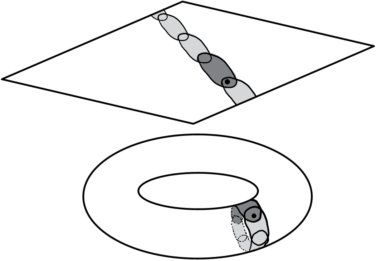
Figure 1. The region $U$ (highlighted in darker gray) is pushed back to itself in the torus by iterates of the translation $\alpha$, but lifting the situation to the plane gives a situation with identical local behavior such that $U$ never returns to itself after leaving

Our goal is, in essence, to construct a geometry that is generated “as freely as possible” by the local behavior of $\alpha$. In other words, we would like to construct a geometry by taking iterates of $U$ under $\alpha$ and gluing them together as little as possible to still retain an automorphism with the same local behavior as $\alpha$ near the distinguished point $\mathscr{e}$.

To specify these iterates in a way that avoids implicitly gluing them inside $\mathscr{G}$, we define, for each $i\in\mathbb{Z}$, a relabeling map

$$\tilde{\alpha}^{i}:q_{{}_{H}}^{-1}(U)\to\tilde{\alpha}^{i}(q_{{}_{H}}^{-1}(U)),$$

where $\tilde{\alpha}^{i}(q_{{}_{H}}^{-1}(U))$ is a diffeomorphic copy of $q_{{}_{H}}^{-1}(U)$ with all of its points $\mathscr{g}$ rewritten as $\tilde{\alpha}^{i}(\mathscr{g})$. There is a natural right $H$-action on $\tilde{\alpha}^{i}(q_{{}_{H}}^{-1}(U))$ given by, for each $h\in H$, $\tilde{\alpha}^{i}(\mathscr{g})h:=\tilde{\alpha}^{i}(\mathscr{g}h)$, which makes $\tilde{\alpha}^{i}$ an $H$-equivariant map and, therefore, an isomorphism of principal $H$-bundles.

With this notation, we can specify what we are doing a bit more concretely. We will take the disjoint union $\bigsqcup_{i\in\mathbb{Z}}\tilde{\alpha}^{i}(q_{{}_{H}}^{-1}(U))$ and apply some minimal gluing (via an equivalence relation $\sim$) to obtain a new Cartan geometry for which $\tilde{\alpha}:\tilde{\alpha}^{i}(\mathscr{g})\mapsto\tilde{\alpha}^{i+1}(\mathscr{g})$ is an automorphism with the same local behavior as $\alpha$ near $\mathscr{e}$. Identifying $\tilde{\alpha}^{0}(q_{{}_{H}}^{-1}(U))$ with $q_{{}_{H}}^{-1}(U)$, so that we may think of $\tilde{\alpha}^{0}(\mathscr{e})\in\tilde{\alpha}^{0}(q_{{}_{H}}^{-1}(U))$ as $\mathscr{e}\in q_{{}_{H}}^{-1}(U)$, this amounts to requiring $\tilde{\alpha}(\mathscr{e})=\alpha(\mathscr{e})$, since automorphisms of Cartan geometries over a connected base manifold are uniquely determined by their image on a single element.

If $\tilde{\alpha}^{i+1}(\mathscr{e})=\tilde{\alpha}^{i}(\tilde{\alpha}(\mathscr{e}))=\tilde{\alpha}^{i}(\alpha(\mathscr{e}))$, then for every (piecewise smooth) path $\gamma:[0,1]\to q_{{}_{H}}^{-1}(U\cap\alpha(U))$ starting with $\alpha(\mathscr{e})$, we must also have $\tilde{\alpha}^{i+1}(\alpha^{-1}(\gamma(t)))=\tilde{\alpha}^{i}(\gamma(t))$ for all $t\in[0,1]$, since $\tilde{\alpha}^{i+1}(\alpha^{-1}(\gamma))$ and $\tilde{\alpha}^{i}(\gamma)$ are paths with the same development and starting point. In other words, whatever this new Cartan geometry is, we must have adjacent iterates $\tilde{\alpha}^{i}(q_{{}_{H}}^{-1}(U))$ and $\tilde{\alpha}^{i+1}(q_{{}_{H}}^{-1}(U))$ glued together by identifying $\tilde{\alpha}^{i}(\mathscr{g})$ with $\tilde{\alpha}^{i+1}(\alpha^{-1}(\mathscr{g}))$ whenever $q_{{}_{H}}(\mathscr{g})$ lies in the connected component of $U\cap\alpha(U)$ containing $\alpha(q_{{}_{H}}(\mathscr{e}))$. With this in mind, it is tempting to imagine that the minimal equivalence relation on $\bigsqcup_{i\in\mathbb{Z}}\tilde{\alpha}^{i}(q_{{}_{H}}^{-1}(U))$ that accomplishes these identifications between adjacent iterates is sufficient as well. Indeed, we can see that this gluing gives precisely the right answer in the torus example given above.

Unfortunately, this naïve gluing will not work in general. To see this, consider the Klein geometry $(\operatorname{\mathrm{I}}(2),\omega_{{}_{\operatorname{\mathrm{I}}(2)}})$ of type $(\operatorname{\mathrm{I}}(2),\operatorname{\mathrm{O}}(2))$ over $\mathbb{R}^{2}$, corresponding to the Euclidean plane. Within this geometry, we choose a rotation $\alpha$ with infinite order that fixes $0$ and an open set $U$ given by the union of a small open ball centered on $0$ and an open sector of the plane that is disjoint from its image under $\alpha$, as depicted in Figure 2. The identity element $(0,\mathds{1})$, which we take to be our distinguished element, is contained in $q_{{}_{\operatorname{\mathrm{O}}(2)}}^{-1}(U)$, as is $\alpha(0,\mathds{1})$, since $\alpha$ fixes $0$. Under the naïve gluing above, the iterates $\tilde{\alpha}^{i}(q_{{}_{\operatorname{\mathrm{O}}(2)}}^{-1}(U))$ all coincide over the small open ball around $0$, but nowhere else. This becomes a problem whenever $U\cap\alpha^{i}(U)$ has points that lie outside of that small open ball: if $x\in U\cap\alpha^{i}(U)$ lies on the boundary of the open ball, then every neighborhood of $\tilde{\alpha}^{i}(\alpha^{-i}(x))$ must intersect every neighborhood of $\tilde{\alpha}^{0}(x)\cong x$ inside the open ball, so since $\tilde{\alpha}^{i}(\alpha^{-i}(x))$ is not identified with $x$ under the naïve gluing, the resulting space is not even Hausdorff.

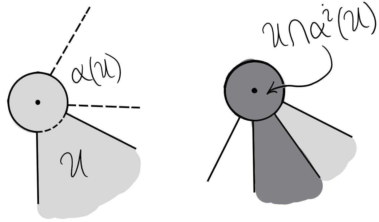
Figure 2. The region $U$ (highlighted in lighter gray) given by the union of an open ball and an open sector that is disjoint from its image under the rotation $\alpha$, as well as a depiction of its intersection (highlighted in darker gray) with an iterate under $\alpha$ where the overlap escapes the open ball

We can, fortunately, salvage this idea with some slightly intricate modifications. Consider a path $\gamma:[0,1]\to U\cap\alpha^{i}(U)$ that starts outside of the open ball and ends inside of it. Then, we get corresponding paths $\tilde{\alpha}^{0}(\gamma)\cong\gamma$ and $\tilde{\alpha}^{i}(\alpha^{-i}(\gamma))$ in $\tilde{\alpha}^{0}(U)$ and $\tilde{\alpha}^{i}(U)$, respectively, and we can lift these to paths $\hat{\gamma}_{0}$ in $\tilde{\alpha}^{0}(q_{{}_{\operatorname{\mathrm{O}}(2)}}^{-1}(U))$ and $\hat{\gamma}_{1}$ in $\tilde{\alpha}^{i}(q_{{}_{\operatorname{\mathrm{O}}(2)}}^{-1}(U))$ with the same development and endpoint. In particular, $\hat{\gamma}_{0}$ and $\hat{\gamma}_{1}$ must coincide inside the new Cartan geometry, if it exists, so that the concatenation $\hat{\gamma}_{0}\star\overline{\hat{\gamma}_{1}}$ of $\hat{\gamma}_{0}$ with the reverse of $\hat{\gamma}_{1}$ is a loop that “backtracks” over itself.

The new strategy, therefore, is to identify elements $\tilde{\alpha}^{i_{1}}(\mathscr{g}_{1})$ and $\tilde{\alpha}^{i_{2}}(\mathscr{g}_{2})$ whenever we can find a path starting at $\alpha^{i_{1}}(\mathscr{g}_{1})$ that only crosses between iterates at points identified under the naïve gluing and which “backtracks” over itself to end up at $\alpha^{i_{2}}(\mathscr{g}_{2})$. In the next subsection, we will formalize this correction to the naïve gluing, which we will use to define the sprawl.

4.2. The definition of the sprawl

To start, we provide a way of describing paths that only cross between iterates at the points identified under the naïve gluing.

Definition 4.1.

A $(U,\alpha,\mathscr{e})$-incrementation for $\gamma:[0,1]\to M$ is a finite partition $0=t_{0}<\cdots<t_{\ell}=1$ of $[0,1]$ together with a finite sequence of integers $k_{0},\dots,k_{\ell-1}\in\mathbb{Z}$ such that, for each $0\leq j<\ell$, $|k_{j}-k_{j+1}|=1$ and $\gamma([t_{j},t_{j+1}])\subseteq\alpha^{k_{j}}(U)$, and for each $0\leq j<\ell-1$, $\gamma(t_{j+1})$ is in the connected component of $\alpha^{k_{j}}(U)\cap\alpha^{k_{j+1}}(U)$ containing $q_{{}_{H}}(\alpha^{\max(k_{j},k_{j+1})}(\mathscr{e}))$. The integers $k_{0}$ and $k_{\ell-1}$ are called the initial label and terminal label, respectively.

Definition 4.2.

We say a path $\gamma:[0,1]\to M$ is $(U,\alpha,\mathscr{e})$-incremented from $i_{1}$ to $i_{2}$ if and only if there is a $(U,\alpha,\mathscr{e})$-incrementation for $\gamma$ with initial label $i_{1}$ and terminal label $i_{2}$.

The basic idea for an incrementation of a path $\gamma$ is to break it into segments $\gamma([t_{j},t_{j+1}])$, and then label each such segment with a specific integer $k_{j}$ such that $\gamma([t_{j},t_{j+1}])\subseteq\alpha^{k_{j}}(U)$. This labeling is further required to only move up or down by $1$ between adjacent segments, with the intersections occurring only in places which must be identified under the naïve gluing. We have attempted to illustrate the concept in Figures 3 and 4.

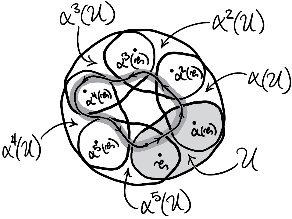
Figure 3. A path $\gamma$, highlighted in darker gray, in the manifold $M$, as well the region $U$, highlighted in lighter gray, and its iterates under an automorphism $\alpha$

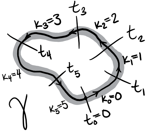
Figure 4. An incrementation for the path $\gamma$ depicted in Figure 3

Recall that a null-homotopy based at a point $q_{{}_{H}}(\mathscr{g})\in M$ is a map $c:[0,1]^{2}\to M$, given as $(s,t)\mapsto c_{s}(t)$, such that

$$c_{s}(0)=c_{s}(1)=c_{1}(s)=q_{{}_{H}}(\mathscr{g})$$

for all $s\in[0,1]$. We will need to use a specific type of homotopy, called a thin homotopy.

Definition 4.3.

A null-homotopy $c:[0,1]^{2}\to M$ is said to be thin if and only if $c([0,1]^{2})=c_{0}([0,1])$. Consequently, a loop $\gamma:[0,1]\to M$ is thinly null-homotopic if and only if there exists a thin null-homotopy $c$ based at $\gamma(0)=\gamma(1)$ such that $c_{0}=\gamma$.

A thin null-homotopy from a loop $\gamma:[0,1]\to M$ to the constant loop at $\gamma(0)=\gamma(1)$ deforms $\gamma$ to a point while staying within its own image. The archetypical example of a thinly null-homotopic loop is the concatenation of a path with its reverse, so that the resulting loop “backtracks” over itself. Thin homotopies are geometrically useful in many contexts because thinly homotopic loops always have the same holonomy (see, for example, [1]). In particular, while we do not make explicit use of this outside of the appendix in the current version of the paper, it is worth noting that thinly null-homotopic loops always have trivial holonomy.

With incrementations and thin null-homotopies in hand, we can now define sprawl-equivalence.

Definition 4.4.

Two points $\tilde{\alpha}^{i_{1}}(q_{{}_{H}}(\mathscr{g}_{1}))$ and $\tilde{\alpha}^{i_{2}}(q_{{}_{H}}(\mathscr{g}_{2}))$ in the disjoint union $\bigsqcup_{i\in\mathbb{Z}}\tilde{\alpha}^{i}(U)$ are sprawl-equivalent (in the base sense) if and only if $\alpha^{i_{1}}(q_{{}_{H}}(\mathscr{g}_{1}))=\alpha^{i_{2}}(q_{{}_{H}}(\mathscr{g}_{2}))$ and there exists a thinly null-homotopic loop $\gamma:[0,1]\to M$ based at $\gamma(0)=q_{{}_{H}}(\alpha^{i_{1}}(\mathscr{g}_{1}))=q_{{}_{H}}(\alpha^{i_{2}}(\mathscr{g}_{2}))=\gamma(1)$ incremented from $i_{1}$ to $i_{2}$.

Definition 4.5.

Two elements $\tilde{\alpha}^{i_{1}}(\mathscr{g}_{1})$ and $\tilde{\alpha}^{i_{2}}(\mathscr{g}_{2})$ of the disjoint union $\bigsqcup_{i\in\mathbb{Z}}\tilde{\alpha}^{i}(q_{{}_{H}}^{-1}(U))$ are sprawl-equivalent (in the bundle sense) if and only if $\alpha^{i_{1}}(\mathscr{g}_{1})=\alpha^{i_{2}}(\mathscr{g}_{2})$ and $\tilde{\alpha}^{i_{1}}(q_{{}_{H}}(\mathscr{g}_{1}))$ is sprawl-equivalent in the base sense to $\tilde{\alpha}^{i_{2}}(q_{{}_{H}}(\mathscr{g}_{2}))$.

Naturally, these notions are related: if $\tilde{\alpha}^{i_{1}}(\mathscr{g}_{1})$ is sprawl-equivalent in the bundle sense to $\tilde{\alpha}^{i_{2}}(\mathscr{g}_{2})$, then $\tilde{\alpha}^{i_{1}}(q_{{}_{H}}(\mathscr{g}_{1}))$ is sprawl-equivalent in the base sense to $\tilde{\alpha}^{i_{2}}(q_{{}_{H}}(\mathscr{g}_{2}))$. In other words, sprawl-equivalence in the bundle sense induces sprawl-equivalence in the base sense; with this justification, we will denote both of them by the same symbol $\sim$. We should, of course, first verify that they are equivalence relations.

Proposition 4.6.

Both notions of sprawl-equivalence are equivalence relations.

Proof.

Let us start with sprawl-equivalence in the base sense, proving that the relation is reflexive, symmetric, and transitive. After this, the proof for the bundle version will follow easily.

For each $i\in\mathbb{Z}$ and $q_{{}_{H}}(\mathscr{g})\in U$, choosing $\gamma$ to be the constant path at $\alpha^{i}(q_{{}_{H}}(\mathscr{g}))$, our partition to be the trivial partition $0=t_{0}<t_{1}=1$, and $i=k_{0}=i$ shows us that $\tilde{\alpha}^{i}(q_{{}_{H}}(\mathscr{g}))\sim\tilde{\alpha}^{i}(q_{{}_{H}}(\mathscr{g}))$.

By definition, if $\tilde{\alpha}^{i_{1}}(q_{{}_{H}}(\mathscr{g}_{1}))\sim\tilde{\alpha}^{i_{2}}(q_{{}_{H}}(\mathscr{g}_{2}))$, then there must be a thinly null-homotopic loop $\gamma:[0,1]\to M$ based at

$$\gamma(0)=q_{{}_{H}}(\alpha^{i_{1}}(\mathscr{g}_{1}))=q_{{}_{H}}(\alpha^{i_{2}}(\mathscr{g}_{2}))=\gamma(1)$$

with an incrementation given by a partition $0=t_{0}<\cdots<t_{\ell}=1$ and a sequence of integers $i_{1}=k_{0},\dots,k_{\ell-1}=i_{2}\in\mathbb{Z}$. Consider the reverse loop $\bar{\gamma}:[0,1]\to M$ defined by $t\mapsto\gamma(1-t)$; setting $\bar{t}_{j}=1-t_{\ell-j}$ and $\bar{k}_{j}=k_{\ell-1-j}$ for each $j$, we get a reversed incrementation from $i_{2}$ to $i_{1}$ for the thinly null-homotopic loop $\bar{\gamma}$, so $\tilde{\alpha}^{i_{2}}(q_{{}_{H}}(\mathscr{g}_{2}))\sim\tilde{\alpha}^{i_{1}}(q_{{}_{H}}(\mathscr{g}_{1}))$.

Similarly, if we have sprawl-equivalences $\tilde{\alpha}^{i_{1}}(q_{{}_{H}}(\mathscr{g}_{1}))\sim\tilde{\alpha}^{i_{2}}(q_{{}_{H}}(\mathscr{g}_{2}))$ and $\tilde{\alpha}^{i_{2}}(q_{{}_{H}}(\mathscr{g}_{2}))\sim\tilde{\alpha}^{i_{3}}(q_{{}_{H}}(\mathscr{g}_{3}))$, then there exist corresponding thinly null-homotopic loops $\gamma$ and $\gamma^{\prime}$, together with incrementations given by $0=t_{0}<\cdots<t_{\ell}=1$ and $i_{1}=k_{0},\dots,k_{\ell-1}=i_{2}\in\mathbb{Z}$ for $\gamma$, and $0=t^{\prime}_{0}<\cdots<t^{\prime}_{\ell^{\prime}}=1$ and $i_{2}=k^{\prime}_{0},\dots,k^{\prime}_{\ell^{\prime}-1}=i_{3}\in\mathbb{Z}$ for $\gamma^{\prime}$. To show that $\tilde{\alpha}^{i_{1}}(q_{{}_{H}}(\mathscr{g}_{1}))\sim\tilde{\alpha}^{i_{3}}(q_{{}_{H}}(\mathscr{g}_{3}))$, consider the concatenated loop $\gamma\star\gamma^{\prime}$. This is still thinly null-homotopic, and setting

$$\tau_{j}=\begin{cases}\frac{t_{j}}{2}&\text{if }j<\ell,\\ \frac{1+t^{\prime}_{j-\ell}}{2}&\text{if }j\geq\ell\end{cases}$$

and

$$r_{j}=\begin{cases}k_{j}&\text{if }j<\ell,\\ k^{\prime}_{j-\ell+1}&\text{if }j\geq\ell\end{cases}$$

for each $j$, we get an incrementation for the concatenation $\gamma\star\gamma^{\prime}$ comprised of the partition $0=\tau_{0}<\cdots<\tau_{\ell+\ell^{\prime}}=1$ and labels $i_{1}=r_{0},\dots,r_{\ell+\ell^{\prime}-1}=i_{3}\in\mathbb{Z}$. In particular, $\tilde{\alpha}^{i_{1}}(q_{{}_{H}}(\mathscr{g}_{1}))\sim\tilde{\alpha}^{i_{3}}(q_{{}_{H}}(\mathscr{g}_{3}))$.

Thus, sprawl-equivalence in the base sense is an equivalence relation, and the proof for the bundle version essentially follows from this. For each $i\in\mathbb{Z}$ and $\mathscr{g}\in q_{{}_{H}}^{-1}(U)$, $\alpha^{i}(\mathscr{g})=\alpha^{i}(\mathscr{g})$ and $\tilde{\alpha}^{i}(q_{{}_{H}}(\mathscr{g}))\sim\tilde{\alpha}^{i}(q_{{}_{H}}(\mathscr{g}))$ by the above, so $\tilde{\alpha}^{i}(\mathscr{g})\sim\tilde{\alpha}^{i}(\mathscr{g})$. Likewise, $\tilde{\alpha}^{i_{1}}(\mathscr{g}_{1})\sim\tilde{\alpha}^{i_{2}}(\mathscr{g}_{2})$ if and only if $\alpha^{i_{1}}(\mathscr{g}_{1})=\alpha^{i_{2}}(\mathscr{g}_{2})$ and $\tilde{\alpha}^{i_{1}}(q_{{}_{H}}(\mathscr{g}_{1}))\sim\tilde{\alpha}^{i_{2}}(q_{{}_{H}}(\mathscr{g}_{2}))$, so $\alpha^{i_{2}}(\mathscr{g}_{2})=\alpha^{i_{1}}(\mathscr{g}_{1})$ and, because sprawl-equivalence in the base sense is symmetric, $\tilde{\alpha}^{i_{2}}(q_{{}_{H}}(\mathscr{g}_{2}))\sim\tilde{\alpha}^{i_{1}}(q_{{}_{H}}(\mathscr{g}_{1}))$, so $\tilde{\alpha}^{i_{2}}(\mathscr{g}_{2})\sim\tilde{\alpha}^{i_{1}}(\mathscr{g}_{1})$. Finally, if we have $\tilde{\alpha}^{i_{1}}(\mathscr{g}_{1})\sim\tilde{\alpha}^{i_{2}}(\mathscr{g}_{2})$ and $\tilde{\alpha}^{i_{2}}(\mathscr{g}_{2})\sim\tilde{\alpha}^{i_{3}}(\mathscr{g}_{3})$, then

$$\alpha^{i_{1}}(\mathscr{g}_{1})=\alpha^{i_{2}}(\mathscr{g}_{2})=\alpha^{i_{3}}(\mathscr{g}_{3})$$

and

$$\tilde{\alpha}^{i_{1}}(q_{{}_{H}}(\mathscr{g}_{1}))\sim\tilde{\alpha}^{i_{2}}(q_{{}_{H}}(\mathscr{g}_{2}))\sim\tilde{\alpha}^{i_{3}}(q_{{}_{H}}(\mathscr{g}_{3})),$$

so by transitivity of the base version, we get $\tilde{\alpha}^{i_{1}}(\mathscr{g}_{1})\sim\tilde{\alpha}^{i_{3}}(\mathscr{g}_{3})$.∎

Sprawl-equivalence is precisely the corrected minimal gluing that we mentioned at the start of the section; as we shall see shortly, it allows us to glue the copies $\tilde{\alpha}^{i}(q_{{}_{H}}^{-1}(U))$ together into a new principal $H$-bundle $\mathscr{F}$ such that $\tilde{\alpha}(\mathscr{e})$ coincides with $\alpha(\mathscr{e})$.

Proposition 4.7.

The quotient space

$$\mathscr{F}=\mathscr{F}(q_{{}_{H}}^{-1}(U),\alpha,\mathscr{e}):=\left(\bigsqcup_{i\in\mathbb{Z}}\tilde{\alpha}^{i}(q_{{}_{H}}^{-1}(U))\right){\Big{/}}\sim$$

admits the structure of a (smooth) principal $H$-bundle over the quotient space

$$q_{{}_{H}}(\mathscr{F})=q_{{}_{H}}(\mathscr{F})(U,\alpha,\mathscr{e}):=\left(\bigsqcup_{i\in\mathbb{Z}}\tilde{\alpha}^{i}(U)\right){\Big{/}}\sim\leavevmode\nobreak\ ,$$

which is a smooth manifold.

Proof.

For each $i\in\mathbb{Z}$, $\tilde{\alpha}^{i}(\mathscr{g}_{1})\sim\tilde{\alpha}^{i}(\mathscr{g}_{2})$ if and only if $\mathscr{g}_{1}=\mathscr{g}_{2}$. In particular, each $\tilde{\alpha}^{i}(q_{{}_{H}}^{-1}(U))$ is embedded in $\mathscr{F}$ under the quotient by $\sim$, so it makes sense to identify each $\tilde{\alpha}^{i}(q_{{}_{H}}^{-1}(U))$ with its image in $\mathscr{F}$. Similarly, each $\tilde{\alpha}^{i}(U)$ naturally embeds into $q_{{}_{H}}(\mathscr{F})$, so we can identify each $\tilde{\alpha}^{i}(U)$ with its image in the quotient space $q_{{}_{H}}(\mathscr{F})$.

For every element $h\in H$, we have $\tilde{\alpha}^{i_{1}}(\mathscr{g}_{1})\sim\tilde{\alpha}^{i_{2}}(\mathscr{g}_{2})$ if and only if $\tilde{\alpha}^{i_{1}}(\mathscr{g}_{1})h\sim\tilde{\alpha}^{i_{2}}(\mathscr{g}_{2})h$, and $\tilde{\alpha}^{i}(\mathscr{g})\sim\tilde{\alpha}^{i}(\mathscr{g})h$ if and only if $h$ is the identity element because otherwise $\alpha^{i}(\mathscr{g})\neq\alpha^{i}(\mathscr{g})h$. Because of this, $\mathscr{F}$ inherits a free right $H$-action that coincides with the smooth free right action of $H$ on each $\tilde{\alpha}^{i}(q_{{}_{H}}^{-1}(U))$. Since $\tilde{\alpha}^{i_{1}}(\mathscr{g}_{1})\sim\tilde{\alpha}^{i_{2}}(\mathscr{g}_{2})$ implies $\tilde{\alpha}^{i_{1}}(q_{{}_{H}}(\mathscr{g}_{1}))\sim\tilde{\alpha}^{i_{2}}(q_{{}_{H}}(\mathscr{g}_{2}))$, we get a natural map $q_{{}_{H}}:\mathscr{F}\to q_{{}_{H}}(\mathscr{F})$ given by $q_{{}_{H}}(\tilde{\alpha}^{i}(\mathscr{g})):=\tilde{\alpha}^{i}(q_{{}_{H}}(\mathscr{g}))$. By definition, this coincides with the bundle map $q_{{}_{H}}:\tilde{\alpha}^{i}(q_{{}_{H}}^{-1}(U))\to\tilde{\alpha}^{i}(U)$ for each $i$, so $\mathscr{F}$ is a principal $H$-bundle over $q_{{}_{H}}(\mathscr{F})$.

It remains to show that $q_{{}_{H}}(\mathscr{F})$ is a smooth manifold. Note that $U$ naturally inherits a smooth structure from $M$, and $q_{{}_{H}}(\mathscr{F})$ is a union of embedded copies of $U$ by definition. Moreover, $\tilde{\alpha}^{i_{1}}(\mathscr{g}_{1})\sim\tilde{\alpha}^{i_{2}}(\mathscr{g}_{2})$ implies $\alpha^{i_{1}}(\mathscr{g}_{1})=\alpha^{i_{2}}(\mathscr{g}_{2})$, hence $\mathscr{g}_{2}=\alpha^{i_{1}-i_{2}}(\mathscr{g}_{1})$, so the embedded copies of $U$ are glued together in $q_{{}_{H}}(\mathscr{F})$ along open sets by iterates of the diffeomorphism $\alpha$. In particular, we just need to show that $q_{{}_{H}}(\mathscr{F})$ is Hausdorff to verify that it admits the structure of a smooth manifold.

To this end, suppose that $\tilde{\alpha}^{i_{1}}(q_{{}_{H}}(\mathscr{g}_{1}))$ and $\tilde{\alpha}^{i_{2}}(q_{{}_{H}}(\mathscr{g}_{2}))$ are distinct points of the quotient space $q_{{}_{H}}(\mathscr{F})$. There are two possible cases: either $\alpha^{i_{1}}(q_{{}_{H}}(\mathscr{g}_{1}))\neq\alpha^{i_{2}}(q_{{}_{H}}(\mathscr{g}_{2}))$, or $\alpha^{i_{1}}(q_{{}_{H}}(\mathscr{g}_{1}))=\alpha^{i_{2}}(q_{{}_{H}}(\mathscr{g}_{2}))$ but no corresponding thinly null-homotopic loop incremented from $i_{1}$ to $i_{2}$ exists. In the first case, there exist disjoint open neighborhoods $V_{1}\subseteq\alpha^{i_{1}}(U)$ of $\alpha^{i_{1}}(q_{{}_{H}}(\mathscr{g}_{1}))$ and $V_{2}\subseteq\alpha^{i_{2}}(U)$ of $\alpha^{i_{2}}(q_{{}_{H}}(\mathscr{g}_{2}))$ because $M$ is Hausdorff, hence $\tilde{\alpha}^{i_{1}}(\alpha^{-i_{1}}(V_{1}))$ and $\tilde{\alpha}^{i_{2}}(\alpha^{-i_{2}}(V_{2}))$ are disjoint open neighborhoods of $\tilde{\alpha}^{i_{1}}(q_{{}_{H}}(\mathscr{g}_{1}))$ and $\tilde{\alpha}^{i_{2}}(q_{{}_{H}}(\mathscr{g}_{2}))$, respectively. In the second case, let $V$ be the path component of the point $\alpha^{i_{1}}(q_{{}_{H}}(\mathscr{g}_{1}))=\alpha^{i_{2}}(q_{{}_{H}}(\mathscr{g}_{2}))$ in the intersection $\alpha^{i_{1}}(U)\cap\alpha^{i_{2}}(U)$, so that $\tilde{\alpha}^{i_{1}}(\alpha^{-i_{1}}(V))$ is an open neighborhood of $\tilde{\alpha}^{i_{1}}(q_{{}_{H}}(\mathscr{g}_{1}))$ and $\tilde{\alpha}^{i_{2}}(\alpha^{-i_{2}}(V))$ is an open neighborhood of $\tilde{\alpha}^{i_{2}}(q_{{}_{H}}(\mathscr{g}_{2}))$. These two neighborhoods must be disjoint: if there were a point $q_{{}_{H}}(\mathscr{f})$ in their intersection, then there would be a path

$$\zeta:[0,1]\to V\subseteq\alpha^{i_{1}}(U)\cap\alpha^{i_{2}}(U)$$

from $\alpha^{i_{1}}(q_{{}_{H}}(\mathscr{g}_{1}))=(\alpha^{i_{1}}\circ(\tilde{\alpha}^{i_{1}})^{-1})(\tilde{\alpha}^{i_{1}}(q_{{}_{H}}(\mathscr{g}_{1})))$ to $(\alpha^{i_{1}}\circ(\tilde{\alpha}^{i_{1}})^{-1})(q_{{}_{H}}(\mathscr{f}))$, so if $\gamma$ were the thinly null-homotopic loop based at

$$(\alpha^{i_{1}}\circ(\tilde{\alpha}^{i_{1}})^{-1})(q_{{}_{H}}(\mathscr{f}))=(\alpha^{i_{2}}\circ(\tilde{\alpha}^{i_{2}})^{-1})(q_{{}_{H}}(\mathscr{f}))$$

incremented from $i_{1}$ to $i_{2}$ that must exist for the point $q_{{}_{H}}(\mathscr{f})$ to be in the intersection of $\tilde{\alpha}^{i_{1}}(U)$ and $\tilde{\alpha}^{i_{2}}(U)$, then the concatenation given by $\zeta\star\gamma\star\bar{\zeta}$ would be a thinly null-homotopic loop based at the point $\alpha^{i_{1}}(q_{{}_{H}}(\mathscr{g}_{1}))=\alpha^{i_{2}}(q_{{}_{H}}(\mathscr{g}_{2}))$ and incremented from $i_{1}$ to $i_{2}$. This would be a contradiction, since $\tilde{\alpha}^{i_{1}}(q_{{}_{H}}(\mathscr{g}_{1}))$ and $\tilde{\alpha}^{i_{2}}(q_{{}_{H}}(\mathscr{g}_{2}))$ are distinct by assumption, so $\tilde{\alpha}^{i_{1}}(\alpha^{-i_{1}}(V))$ and $\tilde{\alpha}^{i_{2}}(\alpha^{-i_{2}}(V))$ must be disjoint. Thus, $q_{{}_{H}}(\mathscr{F})$ is Hausdorff.∎

To imbue this new principal $H$-bundle with the structure of a Cartan geometry, we will use a natural map from $\mathscr{F}$ to $\mathscr{G}$ in order to pull the Cartan connection on $\mathscr{G}$ back to $\mathscr{F}$. This map, called the sprawl map, is precisely the one obtained by identifying each $\tilde{\alpha}^{i}(q_{{}_{H}}^{-1}(U))$ embedded in $\mathscr{F}$ with the corresponding $\alpha^{i}(q_{{}_{H}}^{-1}(U))$ in $\mathscr{G}$.

Definition 4.8.

The map $\sigma:\mathscr{F}\to\mathscr{G}$ given by $\tilde{\alpha}^{i}(\mathscr{g})\mapsto\alpha^{i}(\mathscr{g})$ is called the sprawl map for $(\mathscr{G},\omega)$.

Before moving on to defining the sprawl, let us make two observations about the sprawl map. First, $\sigma$ is well-defined: $\tilde{\alpha}^{i_{1}}(\mathscr{g}_{1})\sim\tilde{\alpha}^{i_{2}}(\mathscr{g}_{2})$ only if $\sigma(\tilde{\alpha}^{i_{1}}(\mathscr{g}_{1}))=\alpha^{i_{1}}(\mathscr{g}_{1})=\alpha^{i_{2}}(\mathscr{g}_{2})=\sigma(\tilde{\alpha}^{i_{2}}(\mathscr{g}_{2}))$, so sprawl-equivalent elements have the same image under $\sigma$. Second, $\sigma$ is an $H$-equivariant local diffeomorphism, since it coincides with the natural $H$-equivariant diffeomorphism between $\tilde{\alpha}^{i}(q_{{}_{H}}^{-1}(U))$ and $\alpha^{i}(q_{{}_{H}}^{-1}(U))$ for each $i\in\mathbb{Z}$.

With that, we can finally define the sprawl.

Definition 4.9.

The sprawl of $(q_{{}_{H}}^{-1}(U),\omega)$ generated by $\alpha$ from $\mathscr{e}$ is the Cartan geometry $(\mathscr{F},\sigma^{*}\omega)$ of type $(G,H)$ over $q_{{}_{H}}(\mathscr{F})$, where $\sigma$ is the sprawl map.

Crucially, note that we have constructed $(\mathscr{F},\sigma^{*}\omega)$ in such a way as to make the map

$$\tilde{\alpha}:\mathscr{F}\to\mathscr{F},\,\tilde{\alpha}^{i}(\mathscr{g})\mapsto\tilde{\alpha}^{i+1}(\mathscr{g})$$

into an automorphism. Indeed, $\sigma$ naturally satisfies $\sigma\circ\tilde{\alpha}=\alpha\circ\sigma$, so

$$\tilde{\alpha}^{*}(\sigma^{*}\omega)=(\sigma\circ\tilde{\alpha})^{*}\omega=(\alpha\circ\sigma)^{*}\omega=\sigma^{*}(\alpha^{*}\omega)=\sigma^{*}\omega.$$

Moreover, $\tilde{\alpha}$ and $\alpha$ must coincide on the distinguished element $\mathscr{e}$ under the identification between $\tilde{\alpha}^{0}(q_{{}_{H}}^{-1}(U))$ and $q_{{}_{H}}^{-1}(U)$, so $\tilde{\alpha}$ has the same local behavior as $\alpha$ on $q_{{}H}^{-1}(U)$ near $\mathscr{e}$.

4.3. The universal property of sprawls

We would like to think of the automorphism $\tilde{\alpha}$ on the sprawl $(\mathscr{F},\sigma^{*}\omega)$ as a kind of universal example of an automorphism with the same behavior as $\alpha$ near $\mathscr{e}$. Theorem 4.12 will make precise what we mean by “universal example”, but first, we will need two lemmas.

First, we need to show that lifts of incremented paths to $\mathscr{G}$ further lift to paths on $\mathscr{F}$ via the sprawl map, and that the choice of lift only depends on the initial label of the underlying incrementation.

Lemma 4.10.

If $\gamma:[0,1]\to\mathscr{G}$ is a path in $\mathscr{G}$ such that its image $q_{{}_{H}}(\gamma)$ in $M$ has an incrementation, then there exists a lift $\tilde{\gamma}:[0,1]\to\mathscr{F}$ of $\gamma$, so that $\sigma\circ\tilde{\gamma}=\gamma$. Moreover, this choice of lift only depends on the initial label of the incrementation of $q_{{}_{H}}(\gamma)$.

Proof.

Suppose that the incrementation of $q_{{}_{H}}(\gamma)$ is the one given by the partition $0=t_{0}<\cdots<t_{\ell}=1$ and labels $k_{0},\dots,k_{\ell-1}\in\mathbb{Z}$. We can construct a path $\tilde{\gamma}$ in $\mathscr{F}$ as follows. First, let us direct our attention to $\alpha^{k_{0}}(q_{{}_{H}}^{-1}(U))$, where the path $\gamma$ starts. When restricted to $\tilde{\alpha}^{k_{0}}(q_{{}_{H}}^{-1}(U))$, $\sigma$ coincides with the identification between $\tilde{\alpha}^{k_{0}}(q_{{}_{H}}^{-1}(U))$ and $\alpha^{k_{0}}(q_{{}_{H}}^{-1}(U))$, so we can simply define

$$\tilde{\gamma}|_{[0,t_{1}]}:=(\sigma|_{\tilde{\alpha}^{k_{0}}(q_{{}_{H}}^{-1}(U))})^{-1}\circ\gamma|_{[0,t_{1}]}.$$

Next, the incrementation tells us that $q_{{}_{H}}(\gamma(t_{1}))$ is in the connected component of $\alpha^{\max(k_{0},k_{1})}(q_{{}_{H}}(\mathscr{e}))$ in $\alpha^{k_{0}}(U)\cap\alpha^{k_{1}}(U)$, so that the constant path at $q_{{}_{H}}(\gamma(t_{1}))$ is a thinly null-homotopic loop incremented from $k_{0}$ to $k_{1}$. In particular, this tells us that $\tilde{\gamma}(t_{1})\in\tilde{\alpha}^{k_{0}}(q_{{}_{H}}^{-1}(U))\cap\tilde{\alpha}^{k_{1}}(q_{{}_{H}}^{-1}(U))$, so that we can extend the path $\tilde{\gamma}$ by again restricting to where $\sigma$ is a diffeomorphism:

$$\tilde{\gamma}|_{[t_{1},t_{2}]}:=(\sigma|_{\tilde{\alpha}^{k_{1}}(q_{{}_{H}}^{-1}(U))})^{-1}\circ\gamma|_{[t_{1},t_{2}]}.$$

By iterating this procedure, defining

$$\tilde{\gamma}|_{[t_{j},t_{j+1}]}:=(\sigma|_{\tilde{\alpha}^{k_{j}}(q_{{}_{H}}^{-1}(U))})^{-1}\circ\gamma|_{[t_{j},t_{j+1}]}$$

for each $j$, we get a well-defined lift $\tilde{\gamma}$ of $\gamma$ to $\mathscr{F}$, with $\sigma\circ\tilde{\gamma}=\gamma$.

Now, suppose that $\zeta:[0,1]\to\mathscr{F}$ is another lift of $\gamma$ to $\mathscr{F}$, constructed in the same way from a possibly different incrementation of $q_{{}_{H}}(\gamma)$. Then, by definition, we would again have $\sigma\circ\zeta=\gamma$, and since $\sigma$ is a geometric map, this means that $\zeta$, $\tilde{\gamma}$, and $\gamma$ would all have the same development: $\zeta_{G}=\tilde{\gamma}_{G}=\gamma_{G}$. In particular, since the starting points of $\zeta$ and $\tilde{\gamma}$ are uniquely determined by the initial label for $q_{{}_{H}}(\gamma)$, we must have $\zeta=\tilde{\gamma}$ if their corresponding incrementations have the same initial label, since then they have the same starting point and the same developments.∎

Our second lemma shows us that development completely determines whether or not a path is a thinly null-homotopic loop.

Lemma 4.11.

A path $\gamma:[0,1]\to\mathscr{G}$ is a thinly null-homotopic loop if and only if its development $\gamma_{G}:[0,1]\to G$ is.

Proof.

Suppose $\gamma$ is a thinly null-homotopic loop in $\mathscr{G}$. Up to smooth reparametrization, we may assume that both $\gamma$ and the thin null-homotopy $c:[0,1]^{2}\to\mathscr{G}$ are smooth. Because $c$ is thin, the image of $c$ is at most one-dimensional, so $c^{*}\omega$ satisfies $\mathrm{d}(c^{*}\omega)+\frac{1}{2}[c^{*}\omega,c^{*}\omega]=0$. By the fundamental theorem of nonabelian calculus (Theorem 7.14 in Chapter 3 of [13]), it follows that there is a unique smooth map $c_{G}:[0,1]^{2}\to G$ such that both $(c_{G})_{0}(0)=e$ and $c_{G}^{*}\omega_{{}_{G}}=c^{*}\omega$; because $\gamma=c_{0}$ and $\gamma_{G}(0)=e=(c_{G})_{0}(0)$, this must also satisfy $(c_{G})_{0}=\gamma_{G}$. Since $c_{G}([0,1]^{2})=(c_{G})_{0}([0,1])$ and $c_{G}$ is constant along $[0,1]\times\{0\}$, $\{1\}\times[0,1]$, and $[0,1]\times\{1\}$, we see that $c_{G}$ is a thin null-homotopy from $\gamma_{G}$ to the constant path at $e$.

Conversely, suppose $\gamma_{G}$ is a thinly null-homotopic loop. Again, up to smooth reparametrization, we may assume that both $\gamma$ and the thin null-homotopy $c_{G}:[0,1]^{2}\to G$ with $(c_{G})_{0}=\gamma_{G}$ are smooth. Our strategy is essentially to just modify the local version of the fundamental theorem of nonabelian calculus to show that a map $c:[0,1]^{2}\to\mathscr{G}$ with $c^{*}\omega=c_{G}^{*}\omega_{{}_{G}}$ exists locally, then build the map from these local pieces starting at $c_{0}(0)=\gamma(0)$. Since such a map $c$ must be constant along $[0,1]\times\{0\}$, $\{1\}\times[0,1]$, and $[0,1]\times\{1\}$, and $(c_{0})_{G}=(c_{G})_{0}=\gamma_{G}$, it will be a null-homotopy from $\gamma$ to $\gamma(0)$ if it exists, and the image of $c$ cannot leave the image of $c_{0}=\gamma$ because the image of $c_{G}$ is contained in the image of $\gamma_{G}$, so $c$ is necessarily a thin null-homotopy.

Emulating the proof of Theorem 6.1 in Chapter 3 of [13], we consider the projections $\pi_{\mathscr{G}}:[0,1]^{2}\times\mathscr{G}\to\mathscr{G}$ and $\pi_{[0,1]^{2}}:[0,1]^{2}\times\mathscr{G}\to[0,1]^{2}$. Setting $\zeta:=(c_{G}\circ\pi_{[0,1]^{2}})^{*}\omega_{{}_{G}}-\pi_{\mathscr{G}}^{*}\omega$, we see that $\pi_{[0,1]^{2}\,*}$ gives a linear isomorphism from $\ker(\zeta)$ to the tangent spaces of $[0,1]^{2}$, so that $\ker(\zeta)$ is a two-dimensional distribution. Moreover, for $\Omega:=\mathrm{d}\omega+\frac{1}{2}[\omega,\omega]$,

$$\mathrm{d}\zeta =(c_{G}\circ\pi_{[0,1]^{2}})^{*}\mathrm{d}\omega_{{}_{G}}-\pi_{\mathscr{G}}^{*}\mathrm{d}\omega$$

$$=-\frac{1}{2}(c_{G}\circ\pi_{[0,1]^{2}})^{*}[\omega_{{}_{G}},\omega_{{}_{G}}]+\frac{1}{2}\pi_{\mathscr{G}}^{*}[\omega,\omega]-\pi_{\mathscr{G}}^{*}\Omega$$

$$=-\frac{1}{2}[\zeta+\pi_{\mathscr{G}}^{*}\omega,\zeta+\pi_{\mathscr{G}}^{*}\omega]+\frac{1}{2}\pi_{\mathscr{G}}^{*}[\omega,\omega]-\pi_{\mathscr{G}}^{*}\Omega$$

$$=-\frac{1}{2}([\zeta,\zeta]+[\pi_{\mathscr{G}}^{*}\omega,\zeta]+[\zeta,\pi_{\mathscr{G}}^{*}\omega])-\pi_{\mathscr{G}}^{*}\Omega.$$

Since $c_{G}$ has rank at most one, $(\pi_{\mathscr{G}})_{*}\ker(\zeta)$ is at most one-dimensional, so $\pi_{\mathscr{G}}^{*}\Omega$ must vanish on $\ker(\zeta)$. The rest of the expression for $\mathrm{d}\zeta$ above is a sum of terms formed by bracketing with $\zeta$, so it must vanish on $\ker(\zeta)$ as well. Thus, $\ker(\zeta)$ is integrable. If $N$ is a leaf of $\ker(\zeta)$ through $((s,t),\mathscr{g})\in[0,1]^{2}\times\mathscr{G}$, then $\pi_{[0,1]^{2}\,*}$ gives a linear isomorphism from the tangent space of $N$ at $((s,t),\mathscr{g})$ to the tangent space of $[0,1]^{2}$ at $(s,t)$, so there is a neighborhood $V$ of $(s,t)$ on which we get a smooth inverse $f:V\to N$ to $\pi_{[0,1]^{2}}$ such that $f(s,t)=((s,t),\mathscr{g})$. Thus,

$$0=f^{*}\zeta =f^{*}((c_{G}\circ\pi_{[0,1]^{2}})^{*}\omega_{{}_{G}}-\pi_{\mathscr{G}}^{*}\omega)$$

$$=f^{*}\pi_{[0,1]^{2}}^{*}(c_{G}^{*}\omega_{{}_{G}})-f^{*}\pi_{\mathscr{G}}^{*}\omega$$

$$=(\pi_{[0,1]^{2}}\circ f)^{*}(c_{G}^{*}\omega_{{}_{G}})-(\pi_{\mathscr{G}}\circ f)^{*}\omega$$

$$=c_{G}^{*}\omega_{{}_{G}}-(\pi_{\mathscr{G}}\circ f)^{*}\omega,$$

so $c|_{V}:=\pi_{\mathscr{G}}\circ f:V\subseteq[0,1]^{2}\to\mathscr{G}$ satisfies $(c|_{V})^{*}\omega=c_{G}^{*}\omega_{{}_{G}}$.

For each $s\in[0,1]$, let $c_{s}:[0,1]\to\mathscr{G}$ be the unique path with $c_{s}(0)=\gamma(0)$ and $(c_{s})_{G}=(c_{G})_{s}$; since $c_{0}=\gamma$ is well-defined and each $c_{s}$ must stay within the image of $c_{0}$, these paths are well-defined as well. If there is a map $c:[0,1]^{2}\to\mathscr{G}$ with $c^{*}\omega=c_{G}^{*}\omega_{{}_{G}}$ and $c_{0}(0)=\gamma(0)$, then it must satisfy $c|_{\{s\}\times[0,1]}=c_{s}$ for each $s$, so we just need to verify that $c:(s,t)\mapsto c_{s}(t)$ works as our map. To do this, choose an open neighborhood $V_{(s,t)}$ for each $(s,t)\in[0,1]^{2}$ such that we get a map $c|_{V_{(s,t)}}$ as above with $(c|_{V_{(s,t)}})(s,t):=c_{s}(t)$ and $(c|_{V_{(s,t)}})^{*}\omega=c_{G}^{*}\omega_{{}_{G}}$. This lets us cover each $\{s\}\times[0,1]$ with open sets on which a map satisfying the desired conditions exists, and these maps $c|_{V_{(s,t)}}$ would necessarily agree on overlaps along $\{s\}\times[0,1]$ because, by definition, $c_{s}$ is the unique path with $c_{s}(0)=\gamma(0)$ and $(c_{s})_{G}=(c_{G})_{s}$. Thus, for each $s\in[0,1]$, setting $V_{s}:=\bigcup_{t\in[0,1]}V_{(s,t)}$, we get a map $c|_{V_{s}}$ on an open neighborhood of $\{s\}\times[0,1]$ such that $(c|_{V_{s}})^{*}\omega=c_{G}^{*}\omega_{{}_{G}}$ and $(c|_{V_{s}})(s,0)=\gamma(0)$. From here, we can glue the maps $c|_{V_{s}}$ together along their overlaps to get $c$, since the $c|_{V_{s}}$ must necessarily coincide on $[0,1]\times\{0\}$ because they are constant along this interval. Thus, we get a map $c:[0,1]^{2}\to\mathscr{G}$ satisfying $c^{*}\omega=c_{G}^{*}\omega_{{}_{G}}$ and $c_{0}(0)=\gamma(0)$, which must be a thin null-homotopy by the argument above.∎

With these lemmas in hand, let us finally explain what the following theorem is meant to tell us. Recall that, in Definition 4.9, we refer to the Cartan geometry $(\mathscr{F},\sigma^{*}\omega)$ as “the sprawl of $(q_{{}_{H}}^{-1}(U),\omega)$ generated by $\alpha$ from $\mathscr{e}$”. Ostensibly, however, $(q_{{}_{H}}^{-1}(U),\omega)$, $\alpha$, and $\mathscr{e}$ are not enough to determine the geometric structure of the sprawl: the Cartan connection is given explicitly in terms of the sprawl map $\sigma$ for $(\mathscr{G},\omega)$, and the topology of $\mathscr{F}$ is determined by particular null-homotopies in $M$. We would like to show that, in truth, the sprawl really is uniquely determined by $(q_{{}_{H}}^{-1}(U),\omega)$, the distinguished element $\mathscr{e}\in q_{{}_{H}}^{-1}(U)$, and the behavior of $\alpha$ on them.

To do this, suppose $(\mathscr{Q},\upsilon)$ is another Cartan geometry of type $(G,H)$ that happens to have an open set geometrically identical to $(q_{{}_{H}}^{-1}(U),\omega)$, meaning that there is a geometric embedding $\psi:(q_{{}_{H}}^{-1}(U),\omega)\hookrightarrow(\mathscr{Q},\upsilon)$. Furthermore, suppose it has an automorphism $\varphi\in\operatorname{\mathrm{Aut}}(\mathscr{Q},\upsilon)$ that behaves exactly as $\alpha$ does on the distinguished element $\mathscr{e}$ under the identification given by the geometric embedding $\psi$; in other words, $\varphi(\psi(\mathscr{e}))=\psi(\alpha(\mathscr{e}))$. Then, if the sprawl truly is uniquely determined by $(q_{{}_{H}}^{-1}(U),\omega)$, $\alpha$, and $\mathscr{e}$, then the sprawl of $(\psi(q_{{}_{H}}^{-1}(U)),\upsilon)$ generated by $\varphi$ from $\psi(\mathscr{e})$ should be geometrically isomorphic to $(\mathscr{F},\sigma^{*}\omega)$ in some natural way. The following theorem shows exactly this; indeed, it shows that the embedding $\psi$ uniquely extends to the new sprawl map for $(\mathscr{Q},\upsilon)$ from $(\mathscr{F},\sigma^{*}\omega)$.

Theorem 4.12.

Let $(\mathscr{Q},\upsilon)$ be another Cartan geometry of type $(G,H)$, with an automorphism $\varphi\in\operatorname{\mathrm{Aut}}(\mathscr{Q},\upsilon)$. If

$$\psi|_{q_{{}_{H}}^{-1}(U)}:(\tilde{\alpha}^{0}(q_{{}_{H}}^{-1}(U)),\sigma^{*}\omega)\cong(q_{{}_{H}}^{-1}(U),\omega)\hookrightarrow(\mathscr{Q},\upsilon)$$

is a geometric embedding such that $\varphi((\psi|_{q_{{}_{H}}^{-1}(U)})(\mathscr{e}))=(\psi|_{q_{{}_{H}}^{-1}(U)})(\alpha(\mathscr{e}))$, then the embedding $\psi|_{q_{{}_{H}}^{-1}(U)}$ has a unique extension to a geometric map $\psi:(\mathscr{F},\sigma^{*}\omega)\to(\mathscr{Q},\upsilon)$ from the sprawl of $(q_{{}_{H}}^{-1}(U),\omega)$ generated by $\alpha$ from $\mathscr{e}$ into $(\mathscr{Q},\upsilon)$ such that $\psi\circ\tilde{\alpha}=\varphi\circ\psi$.

Proof.

If the desired extension to $\mathscr{F}$ exists, then it must be of the form $\psi:\tilde{\alpha}^{i}(\mathscr{g})\mapsto\varphi^{i}((\psi|_{q_{{}_{H}}^{-1}(U)})(\mathscr{g}))$, so uniqueness is immediate and

$$(\psi^{*}\upsilon)_{\tilde{\alpha}^{i}(\mathscr{g})} =\psi^{*}(\upsilon_{\varphi^{i}(\psi(\mathscr{g}))})=\psi^{*}(\varphi^{-i})^{*}(\upsilon_{\psi(\mathscr{g})})=(\varphi^{-i}\circ\psi)^{*}(\upsilon_{\psi(\mathscr{g})})$$

$$=(\psi\circ\tilde{\alpha}^{-i})^{*}(\upsilon_{\psi(\mathscr{g})})=(\tilde{\alpha}^{-i})^{*}\psi^{*}(\upsilon_{\psi(\mathscr{g})})=(\tilde{\alpha}^{-i})^{*}(\sigma^{*}\omega_{\mathscr{g}})$$

$$=(\sigma^{*}\omega)_{\tilde{\alpha}^{i}(\mathscr{g})},$$

hence $\psi$ must be a geometric map as well. Thus, we just need to show that an extension of this form is well-defined.

To this end, suppose $\tilde{\alpha}^{i_{1}}(\mathscr{g}_{1})\sim\tilde{\alpha}^{i_{2}}(\mathscr{g}_{2})$, so that $\alpha^{i_{1}}(\mathscr{g}_{1})=\alpha^{i_{2}}(\mathscr{g}_{2})$ and there exists a thinly null-homotopic loop $q_{{}_{H}}(\gamma):[0,1]\to M$ based at the point $\alpha^{i_{1}}(q_{{}_{H}}(\mathscr{g}_{1}))=\alpha^{i_{2}}(q_{{}_{H}}(\mathscr{g}_{2}))$ incremented from $i_{1}$ to $i_{2}$. Since the image of a null-homotopy is contractible, we can lift $q_{{}_{H}}(\gamma)$ to a thinly null-homotopic loop $\gamma:[0,1]\to\mathscr{G}$ based at $\alpha^{i_{1}}(\mathscr{g}_{1})=\alpha^{i_{2}}(\mathscr{g}_{2})$, and by Lemma 4.10, we can further lift to a path $\tilde{\gamma}:[0,1]\to\mathscr{F}$ starting at $\tilde{\alpha}^{i_{1}}(\mathscr{g}_{1})$. Since $\gamma_{G}=\tilde{\gamma}_{G}$, $\tilde{\gamma}$ is again a thinly null-homotopic loop by Lemma 4.11. Our strategy to show that

$$\psi(\tilde{\alpha}^{i_{1}}(\mathscr{g}_{1}))=\psi(\tilde{\gamma}(0))=\psi(\tilde{\gamma}(1))=\psi(\tilde{\alpha}^{i_{2}}(\mathscr{g}_{2}))$$

is to construct a well-defined path $\beta:[0,1]\to\mathscr{Q}$ that always agrees with what the composite $\psi\circ\tilde{\gamma}$ is if $\psi$ is well-defined; because we will have $\beta_{G}=\tilde{\gamma}_{G}$, $\beta$ will be a thinly null-homotopic loop by Lemma 4.11, hence

$$\psi(\tilde{\gamma}(0))=\beta(0)=\beta(1)=\psi(\tilde{\gamma}(1)).$$

We construct the path $\beta:[0,1]\to\mathscr{Q}$ along the lines of the proof of Lemma 4.10. Let the incrementation of $q_{{}_{H}}(\gamma)$ be given by the partition $0=t_{0}<\cdots<t_{\ell}=1$ and labels $i_{1}=k_{0},\dots,k_{\ell-1}=i_{2}\in\mathbb{Z}$. To start, this means that $\tilde{\gamma}([0,t_{1}])\subseteq\tilde{\alpha}^{i_{1}}(q_{{}_{H}}^{-1}(U))$, since $\sigma(\tilde{\gamma})=\gamma$ by definition. Whenever we restrict $\psi$ to a given $\tilde{\alpha}^{k}(q_{{}_{H}}^{-1}(U))$, we get a well-defined geometric embedding $\psi|_{\tilde{\alpha}^{k}(q_{{}_{H}}^{-1}(U))}$, which by definition is given by

$$\psi|_{\tilde{\alpha}^{k}(q_{{}_{H}}^{-1}(U))}:=\varphi^{k}\circ(\psi|_{q_{{}_{H}}^{-1}(U)})\circ\tilde{\alpha}^{-k}|_{\tilde{\alpha}^{k}(q_{{}_{H}}^{-1}(U))}.$$

Therefore, it is valid to define $\beta|_{[0,t_{1}]}:=\psi|_{\tilde{\alpha}^{i_{1}}(q_{{}_{H}}^{-1}(U))}\circ\tilde{\gamma}|_{[0,t_{1}]}$.

At this point, we make a key observation: because the elements $\tilde{\alpha}(\mathscr{e})$ and $\alpha(\mathscr{e})$ are identified in $(\tilde{\alpha}^{0}(q_{{}_{H}}^{-1}(U)),\sigma^{*}\omega)\cong(q_{{}_{H}}^{-1}(U),\omega)$ and $(\psi|_{q_{{}_{H}}^{-1}(U)})(\tilde{\alpha}(\mathscr{e}))=\varphi((\psi|_{q_{{}_{H}}^{-1}(U)})(\mathscr{e}))$, the geometric embeddings $\psi|_{q_{{}_{H}}^{-1}(U)}$ and

$$\psi|_{\tilde{\alpha}(q_{{}_{H}}^{-1}(U))}=\varphi\circ(\psi|_{q_{{}_{H}}^{-1}(U)})\circ\tilde{\alpha}^{-1}|_{\tilde{\alpha}(q_{{}_{H}}^{-1}(U))}$$

must coincide over the connected component of $q_{{}_{H}}(\tilde{\alpha}(\mathscr{e}))=q_{{}_{H}}(\alpha(\mathscr{e}))$ in the intersection $U\cap\tilde{\alpha}(U)$ in $q_{{}_{H}}(\mathscr{F})$, since

$$(\psi|_{\tilde{\alpha}(q_{{}_{H}}^{-1}(U))})(\tilde{\alpha}(\mathscr{e}))=\varphi((\psi|_{q_{{}_{H}}^{-1}(U)})(\mathscr{e}))=(\psi|_{q_{{}_{H}}^{-1}(U)})(\tilde{\alpha}(\mathscr{e})).$$

Using iterates of $\tilde{\alpha}$ and $\varphi$ to move to the other copies of $q_{{}_{H}}^{-1}(U)$, we see that, for each $k$, $\psi|_{\tilde{\alpha}^{k}(q_{{}_{H}}^{-1}(U))}$ and $\psi|_{\tilde{\alpha}^{k+1}(q_{{}_{H}}^{-1}(U))}$ must coincide over the connected component of $q_{{}_{H}}(\tilde{\alpha}^{k+1}(\mathscr{e}))$ in $\tilde{\alpha}^{k}(U)\cap\tilde{\alpha}^{k+1}(U)$. By definition, the incrementation of $q_{{}_{H}}(\gamma)$ tells us that $q_{{}_{H}}(\gamma)(t_{1})$ lies in the connected component of $\alpha^{\max(k_{0},k_{1})}(q_{{}_{H}}(\mathscr{e}))$ in $\alpha^{k_{0}}(U)\cap\alpha^{k_{1}}(U)$, so $\tilde{\gamma}(t_{1})$ must lie over the connected component of $\tilde{\alpha}^{\max(k_{0},k_{1})}(q_{{}_{H}}(\mathscr{e}))$ in $\tilde{\alpha}^{k_{0}}(U)\cap\tilde{\alpha}^{k_{1}}(U)$. In particular, $\psi|_{\tilde{\alpha}^{k_{0}}(q_{{}_{H}}^{-1}(U))}$ and $\psi|_{\tilde{\alpha}^{k_{1}}(q_{{}_{H}}^{-1}(U))}$ must coincide on $\tilde{\gamma}(t_{1})$ because $|k_{0}-k_{1}|=1$, so we can extend $\beta$ to $[0,t_{2}]$ by defining $\beta|_{[t_{1},t_{2}]}:=\psi|_{\tilde{\alpha}^{k_{1}}(q_{{}_{H}}^{-1}(U))}\circ\tilde{\gamma}|_{[t_{1},t_{2}]}$.

By iterating this procedure, defining

$$\beta|_{[t_{j},t_{j+1}]}:=\psi|_{\tilde{\alpha}^{k_{j}}(q_{{}_{H}}^{-1}(U))}\circ\tilde{\gamma}|_{[t_{j},t_{j+1}]}$$

for each $j$, we get a well-defined path $\beta$ that must be of the form $\psi\circ\tilde{\gamma}$ if the extension $\psi$ is well-defined. In particular, $\beta$ is a path from $\beta(0)=\varphi^{i_{1}}((\psi|_{q_{{}_{H}}^{-1}(U)})(\mathscr{g}_{1}))$ to $\beta(1)=\varphi^{i_{2}}((\psi|_{q_{{}_{H}}^{-1}(U)})(\mathscr{g}_{2}))$ with $\beta_{G}=\tilde{\gamma}_{G}$, so it must be a thinly null-homotopic loop based at

$$\psi(\tilde{\alpha}^{i_{1}}(\mathscr{g}_{1}))=\beta(0)=\beta(1)=\psi(\tilde{\alpha}^{i_{2}}(\mathscr{g}_{2})).\mbox{\qed}$$

This theorem is, as it turns out, remarkably well-suited to placing strong restrictions on which Cartan geometries can admit certain types of automorphisms. As an example, if $(M,\nabla)$ is an affine structure on a connected smooth manifold $M$ and $\alpha$ is an affine transformation of $(M,\nabla)$ that fixes a point $x$ and whose derivative at $x$ just rescales the tangent space at $x$ by some $\lambda\neq\pm 1$, then $(M,\nabla)$ must be isomorphic to the affine structure on affine space.

Corollary 4.13.

Suppose that $(\mathscr{G},\omega)$ is a Cartan geometry of type $(\mathrm{Aff}(m),\operatorname{\mathrm{GL}}_{m}\mathbb{R})$ over a connected smooth manifold $M$ with an automorphism $\alpha\in\operatorname{\mathrm{Aut}}(\mathscr{G},\omega)$ such that, for some $\mathscr{e}\in\mathscr{G}$ and $\lambda\neq\pm 1$, $\alpha(\mathscr{e})=\mathscr{e}(\lambda\mathds{1})$. Then, $(\mathscr{G},\omega)$ is isomorphic to the Klein geometry $(\mathrm{Aff}(m),\omega_{{}_{\mathrm{Aff}(m)}})$ over $\mathbb{R}^{m}$.

Proof.

By considering the inverse of $\alpha$ or squaring if necessary, we may assume that $0<\lambda<1$. As we saw in Section 3, because $\alpha(\mathscr{e})=\mathscr{e}(\lambda\mathds{1})$, $(\mathscr{G},\omega)$ is flat in a neighborhood of $\mathscr{e}$. Therefore, for some connected open neighborhood $U$ of $0$ in $\mathbb{R}^{m}$, we have a geometric embedding

$$\psi:(q_{\operatorname{\mathrm{GL}}_{m}\mathbb{R}}^{-1}(U),\omega_{{}_{\mathrm{Aff}(m)}})\hookrightarrow(\mathscr{G},\omega)$$

such that $\psi(0,\mathds{1})=\mathscr{e}$, and since

$$\alpha(\psi(0,\mathds{1}))=\psi(0,\mathds{1})(\lambda\mathds{1})=\psi(\lambda\mathds{1}\cdot(0,\mathds{1})),$$

Theorem 4.12 tells us that $\psi$ extends to a geometric map from the sprawl of $(q_{\operatorname{\mathrm{GL}}_{m}\mathbb{R}}^{-1}(U),\omega_{{}_{\mathrm{Aff}(m)}})$ from $(0,\mathds{1})$ generated by $\lambda\mathds{1}$.

This sprawl happens to be just the Klein geometry $(\mathrm{Aff}(m),\omega_{{}_{\mathrm{Aff}(m)}})$. To see this, note that $\lambda\mathds{1}$ fixes $0\in\mathbb{R}^{m}$, so the iterates $\widetilde{\lambda\mathds{1}}{}^{k}(U)$ all contain $\widetilde{\lambda\mathds{1}}{}^{0}(0)\cong 0$. Moreover, for all sufficiently large positive $k$, the iterate $(\lambda\mathds{1})^{-k}(U)=\lambda^{-k}\mathds{1}(U)$ will properly contain $U$, so if $\gamma$ is a path in $\widetilde{\lambda\mathds{1}}{}^{0}(q_{{}_{\operatorname{\mathrm{GL}}_{m}\mathbb{R}}}^{-1}(U))\cong q_{{}_{\operatorname{\mathrm{GL}}_{m}\mathbb{R}}}^{-1}(U)$ ending with $(0,\mathds{1})$, $\widetilde{\lambda\mathds{1}}{}^{-k}(q_{{}_{\operatorname{\mathrm{GL}}_{m}\mathbb{R}}}^{-1}(U))$ must contain a path $\gamma^{\prime}$ with the same development also ending at $(0,\mathds{1})$, so $\gamma\star\overline{\gamma^{\prime}}$ is a thinly null-homotopic loop incremented from $0$ to $k$ by Lemma 4.11. In other words, $\widetilde{\lambda\mathds{1}}{}^{0}(q_{{}_{\operatorname{\mathrm{GL}}_{m}\mathbb{R}}}^{-1}(U))\subseteq\widetilde{\lambda\mathds{1}}{}^{-k}(q_{{}_{\operatorname{\mathrm{GL}}_{m}\mathbb{R}}}^{-1}(U))$ for all sufficiently large $k$, hence $\widetilde{\lambda\mathds{1}}{}^{i}(q_{{}_{\operatorname{\mathrm{GL}}_{m}\mathbb{R}}}^{-1}(U))\subseteq\widetilde{\lambda\mathds{1}}{}^{i-k}(q_{{}_{\operatorname{\mathrm{GL}}_{m}\mathbb{R}}}^{-1}(U))$ for all sufficiently large $k$. Since the union of all the $(\lambda\mathds{1})^{-k}(U)$ is $\mathbb{R}^{m}$, this means that $\widetilde{\lambda\mathds{1}}{}^{i_{1}}(v_{1},A_{1})$ and $\widetilde{\lambda\mathds{1}}{}^{i_{2}}(v_{2},A_{2})$ are sprawl-equivalent if and only if $(\lambda\mathds{1})^{i_{1}}(v_{1},A_{1})=(\lambda\mathds{1})^{i_{2}}(v_{2},A_{2})$, so the sprawl is just $(\mathrm{Aff}(m),\omega_{{}_{\mathrm{Aff}(m)}})$.

Since $(\mathrm{Aff}(m),\omega_{{}_{\mathrm{Aff}(m)}})$ is complete, the geometric map $\psi$ must be a covering map. However, if $\Gamma$ is a discrete subgroup of $\mathrm{Aff}(m)$ that is normalized by $\lambda\mathds{1}$, then $\Gamma<\operatorname{\mathrm{GL}}_{m}\mathbb{R}$, so there is no nontrivial covering map to a Cartan geometry with an automorphism having isotropy $\lambda\mathds{1}$. In other words, $\psi$ must be a geometric isomorphism.∎

5. Applications

Here, we will prove Theorems A, B, and C from the introduction. To do this, we will prove a more general result, and then we will show that the hypotheses of this result are satisfied in each of the desired cases.

Throughout this section, we will need a notion of codimension; it will be convenient to use the following terminology.

Definition 5.1.

For a smooth manifold $M$ and a closed subset $N\subseteq M$, we say that $v\in TM$ is not tangent to $N$ if and only if for every path $\gamma:[0,1]\to M$ with $\dot{\gamma}(0)=v$, there exists an $\varepsilon>0$ such that $\gamma((0,\varepsilon))\not\subseteq N$. We will say that $N$ has codimension at least one if and only if, for each $p\in M$, there is a $v\in T_{p}M$ that is not tangent to $N$.

Definition 5.2.

For a smooth manifold $M$, we will say that a closed subset $N\subseteq M$ has codimension at least two if and only if, for each path $\gamma:[0,1]\to M$, we can choose arbitrarily small intervals around each $t_{0}$ for which $\gamma(t_{0})\in N$ and get a homotopy $c:[0,1]^{2}\to M$ with $c_{0}=\gamma$ such that $c((0,1]\times[0,1])\not\subseteq N$ and, for every $s\in[0,1]$, $c_{s}(t)=\gamma(t)$ for all $t$ outside of those small intervals.

Closed submanifolds and subvarieties $N\subseteq M$ will, of course, have codimension at least one if $\dim(M)-\dim(N)\geq 1$ and have codimension at least two if $\dim(M)-\dim(N)\geq 2$.

To consolidate assumptions, we also make the following definitions characterizing the isotropies $a$ for the automorphisms in which we are currently interested.

Definition 5.3.

A flamboyance for $a\in H$ in the model $(G,H)$ is a set $\mathcal{L}$ of $a$-invariant simply connected compact subspaces of $G/H$ for which the following three conditions are satisfied:

• For each $q_{{}_{H}}(g)\not\in\mathrm{Fix}_{G/H}(a)$, there is an $\ell\in\mathcal{L}$ containing $q_{{}_{H}}(g)$;

• For every $\ell\in\mathcal{L}$, $\ell\cap\mathrm{Fix}_{G/H}(a)=\{q_{{}_{H}}(e)\}$;

• For every $\ell,\ell^{\prime}\in\mathcal{L}$, the intersection $\ell\cap\ell^{\prime}$ is path-connected.

Definition 5.4.

We say that $a\in H$ is flamboyant in the model $(G,H)$ if and only if there exists a flamboyance for $a$, $a^{k}(q_{{}_{H}}(g))\rightarrow q_{{}_{H}}(e)$ as $k\rightarrow+\infty$ whenever $q_{{}_{H}}(g)\not\in\mathrm{Fix}_{G/H}(a)$, and the set $\mathrm{Fix}_{G/H}(a)$ of fixed points for $a$ in $G/H$ has codimension at least two.

The idea of a flamboyance will allow us to place certain convenient restrictions on the sprawls generated by an isotropy $a\in H$, as we will see in the next subsection.

5.1. General result

In this subsection, we will prove the following result, from which Theorems A, B, and C will follow.

Theorem 5.5.

Suppose $(\mathscr{G},\omega)$ is a Cartan geometry of type $(G,H)$ over a connected smooth manifold $M$, together with an automorphism $\alpha\in\operatorname{\mathrm{Aut}}(\mathscr{G},\omega)$ and a distinguished element $\mathscr{e}\in\mathscr{G}$ such that $\alpha(\mathscr{e})=\mathscr{e}a$ for some flamboyant $a\in H$. If $(\mathscr{G},\omega)$ is flat in a neighborhood of $\mathscr{e}$, then it geometrically embeds onto a dense open subset of the Klein geometry $(G,\omega_{{}_{G}})$ of type $(G,H)$.

To start the proof, notice that we can get a geometric embedding $\psi:(q_{{}_{H}}^{-1}(U),\omega_{{}_{G}})\hookrightarrow(\mathscr{G},\omega)$ with $\psi(e)=\mathscr{e}$ for all sufficiently small neighborhoods $U$ of $q_{{}_{H}}(e)$ in $G/H$ because the geometry is flat in a neighborhood of $\mathscr{e}$. Since $\alpha(\mathscr{e})=\mathscr{e}a$ and $\psi$ is $H$-equivariant,

$$\psi(ae)=\psi(ea)=\psi(e)a=\alpha(\psi(e)),$$

so by Theorem 4.12, $\psi$ extends to a geometric map from the sprawl $(\mathscr{F},\sigma^{*}\omega_{{}_{G}})$ of $(q_{{}_{H}}^{-1}(U),\omega_{{}_{G}})$ generated by $a$ from $e$ into $(\mathscr{G},\omega)$.

Next, we want to prove that the sprawl map $\sigma:(\mathscr{F},\sigma^{*}\omega_{{}_{G}})\to(G,\omega_{{}_{G}})$ for the Klein geometry is a geometric embedding. To do this, we will use the following two lemmas.

Lemma 5.6.

Suppose $\varphi:(\mathscr{G},\omega)\to(\mathscr{Q},\upsilon)$ is a geometric map and $V\subseteq\mathscr{Q}$ is a dense open subset such that the complement $\mathscr{Q}\setminus V$ has codimension at least one. If $\varphi|_{\varphi^{-1}(V)}$ is injective, then $\varphi$ is injective.

Proof.

Suppose $\varphi(\mathscr{g}_{1})=\varphi(\mathscr{g}_{2})$ for $\mathscr{g}_{1},\mathscr{g}_{2}\in\mathscr{G}$. Choosing $X\in\mathfrak{g}$ such that $\upsilon_{\varphi(\mathscr{g}_{1})}^{-1}(X)=\upsilon_{\varphi(\mathscr{g}_{2})}^{-1}(X)$ is not tangent to $\mathscr{Q}\setminus V$, we have

$$\varphi(\exp(t\omega^{-1}(X))\mathscr{g}_{1}) =\exp(t\upsilon^{-1}(X))\varphi(\mathscr{g}_{1})$$

$$=\exp(t\upsilon^{-1}(X))\varphi(\mathscr{g}_{2})$$

$$=\varphi(\exp(t\omega^{-1}(X))\mathscr{g}_{2})$$

for all $t\in\mathbb{R}$ such that both $\exp(t\omega^{-1}(X))\mathscr{g}_{1}$ and $\exp(t\omega^{-1}(X))\mathscr{g}_{2}$ are well-defined, and for all sufficiently small $t\neq 0$, it is in $V$. Thus,

$$\exp(t\omega^{-1}(X))\mathscr{g}_{1}=\exp(t\omega^{-1}(X))\mathscr{g}_{2}$$

by injectivity of $\varphi|_{\varphi^{-1}(V)}$, hence

$$\mathscr{g}_{1} =\exp(t\omega^{-1}(X))^{-1}\exp(t\omega^{-1}(X))\mathscr{g}_{1}$$

$$=\exp(t\omega^{-1}(X))^{-1}\exp(t\omega^{-1}(X))\mathscr{g}_{2}=\mathscr{g}_{2}.\mbox{\qed}$$

Lemma 5.7.

If $a\in H$ is flamboyant in $(G,H)$, then the sprawl $(\mathscr{F},\sigma^{*}\omega_{{}_{G}})$ of $(q_{{}_{H}}^{-1}(U),\omega_{{}_{G}})$ generated by $a$ from $e$ has injective sprawl map $\sigma:(\mathscr{F},\sigma^{*}\omega_{{}_{G}})\to(G,\omega_{{}_{G}})$.

Proof.

Suppose $\ell$ is an element of a flamboyance $\mathcal{L}$ for $a$, so that $\ell$ is an $a$-invariant simply connected compact subspace of $G/H$ whose only fixed point is $q_{{}_{H}}(e)$. Let $(\ell\cap U)_{0}$ be the path component of $\ell\cap U$ containing $q_{{}_{H}}(e)$; by invariance of $\ell$ and $q_{{}_{H}}(e)$, $a^{k}(\ell\cap U)_{0}=(\ell\cap a^{k}(U))_{0}$. Since $U$ is open, $\ell\setminus(\ell\cap U)_{0}$ is closed, hence compact. Therefore, for all sufficiently large $k$,

$$a^{k}(\ell\setminus(\ell\cap U)_{0})=\ell\setminus(\ell\cap a^{k}(U))_{0}\subseteq(\ell\cap U)_{0},$$

since $a^{k}(q_{{}_{H}}(g))\rightarrow q_{{}_{H}}(e)$ for each $q_{{}_{H}}(g)\not\in\mathrm{Fix}_{G/H}(a)$. In other words,

$$(\ell\cap U)_{0}\cup(\ell\cap a^{k}(U))_{0}=\ell$$

for all sufficiently large $k$. Because $\ell$ is simply connected, $\mathrm{H}_{1}(\ell)=\{0\}$, and by path-connectedness,

$$\mathrm{H}_{0}((\ell\cap U)_{0})\approx\mathrm{H}_{0}((\ell\cap a^{k}(U))_{0})\approx\mathrm{H}_{0}(\ell)\approx\mathbb{Z},$$

so for all sufficiently large $k$, we get a short exact sequence

$$\{0\}\to\mathrm{H}_{0}((\ell\cap U)_{0}\cap(\ell\cap a^{k}(U))_{0})\hookrightarrow\mathbb{Z}\oplus\mathbb{Z}\twoheadrightarrow\mathbb{Z}\to\{0\}$$

by Mayer-Vietoris. It follows that $\mathrm{H}_{0}((\ell\cap U)_{0}\cap(\ell\cap a^{k}(U))_{0})\approx\mathbb{Z}$ as well, so $(\ell\cap U)_{0}\cap(\ell\cap a^{k}(U))_{0}$ is path-connected.

Thus, for every $g_{1},g_{2}\in q_{{}_{H}}^{-1}((\ell\cap U)_{0})$ such that $g_{1}=a^{k}(g_{2})$, there exists a path

$$\zeta:[0,1]\to(\ell\cap U)_{0}\cap(\ell\cap a^{k}(U))_{0}\subseteq\ell\cap U\cap a^{k}(U)$$

with $\zeta(0)=q_{{}_{H}}(g_{1})$ and $\zeta(1)=q_{{}_{H}}(e)$ whenever $k$ is sufficiently large, so the concatenation $\zeta\star\bar{\zeta}$ is a thinly null-homotopic loop incremented from $0$ to $k$ because $q_{{}_{H}}(e)$ is in the connected component of $a^{i}(q_{{}_{H}}(e))=q_{{}_{H}}(e)$ in $a^{i-1}(U)\cap a^{i}(U)$ for every $i$. By definition of sprawl-equivalence, this means that $\tilde{a}^{0}(g_{1})$ is sprawl-equivalent to $\tilde{a}^{k}(g_{2})$ if and only if

$$\sigma(\tilde{a}^{0}(g_{1}))=g_{1}=a^{k}(g_{2})=\sigma(\tilde{a}^{k}(g_{2}))$$

when $g_{1}\in q_{{}_{H}}^{-1}((\ell\cap U)_{0})$ and $a^{k}(g_{2})\in q_{{}_{H}}^{-1}((\ell\cap a^{k}(U))_{0})$. The sprawl map $\sigma$ restricts to an embedding on $\tilde{a}^{0}(q_{{}_{H}}^{-1}(U))$ and $\tilde{a}^{k}(q_{{}_{H}}^{-1}(U))$, so it is injective on both

$$L_{1}:=(\sigma|_{\tilde{a}^{0}(q_{{}_{H}}^{-1}(U))})^{-1}(q_{{}_{H}}^{-1}((\ell\cap U)_{0}))$$

and

$$L_{2}:=(\sigma|_{\tilde{a}^{k}(q_{{}_{H}}^{-1}(U))})^{-1}(q_{{}_{H}}^{-1}((\ell\cap a^{k}(U))_{0})).$$

Since $\sigma(\tilde{a}^{0}(g_{1}))=\sigma(\tilde{a}^{k}(g_{2}))$ if and only if $\tilde{a}^{0}(g_{1})$ is sprawl-equivalent to $\tilde{a}^{k}(g_{2})$, it follows that $\sigma$ is also injective on the union $q_{{}_{H}}^{-1}(\tilde{\ell}):=L_{1}\cup L_{2}$, whose image under $\sigma$ is precisely

$$\sigma(q_{{}_{H}}^{-1}(\tilde{\ell})) =q_{{}_{H}}^{-1}((\ell\cap U)_{0})\cup q_{{}_{H}}^{-1}((\ell\cap a^{k}(U))_{0})$$

$$=q_{{}_{H}}^{-1}((\ell\cap U)_{0}\cup(\ell\cap a^{k}(U))_{0})$$

$$=q_{{}_{H}}^{-1}(\ell).$$

For each $\ell\in\mathcal{L}$, we therefore get a subset $q_{{}_{H}}^{-1}(\tilde{\ell})$ of $\mathscr{F}$ such that the restriction $\sigma|_{q_{{}_{H}}^{-1}(\tilde{\ell})}$ is injective onto $q_{{}_{H}}^{-1}(\ell)$. Moreover, for every $g\in q_{{}_{H}}^{-1}(\ell\cap\ell^{\prime})$ with $\ell,\ell^{\prime}\in\mathcal{L}$, there is a path $\gamma:[0,1]\to q_{{}_{H}}^{-1}(\ell\cap\ell^{\prime})$ such that $\gamma(0)=e$ and $\gamma(1)\in gH$ because $\ell\cap\ell^{\prime}$ is path-connected; the paths $(\sigma|_{q_{{}_{H}}^{-1}(\tilde{\ell})})^{-1}(\gamma)$ and $(\sigma|_{q_{{}_{H}}^{-1}(\tilde{\ell}^{\prime})})^{-1}(\gamma)$ have the same development and both start at $\tilde{a}^{0}(e)$, so they must be the same path, hence $(\sigma|_{q_{{}_{H}}^{-1}(\tilde{\ell})})^{-1}$ and $(\sigma|_{q_{{}_{H}}^{-1}(\tilde{\ell}^{\prime})})^{-1}$ must agree on the intersection $q_{{}_{H}}^{-1}(\ell\cap\ell^{\prime})$. In particular, the restriction of $\sigma$ to the union $W:=\bigcup_{\ell\in\mathcal{L}}q_{{}_{H}}^{-1}(\tilde{\ell})$ is still injective, and the image of $W$ under $\sigma$ contains the complement $G\setminus q_{{}_{H}}^{-1}(\mathrm{Fix}_{G/H}(a))$ because $\mathcal{L}$ is a flamboyance for $a$.

Now, we want to prove that $\sigma$ is injective on $\sigma^{-1}(G\setminus q_{{}_{H}}^{-1}(\mathrm{Fix}_{G/H}(a)))$. Suppose $a^{i}(g)\not\in q_{{}_{H}}^{-1}(\mathrm{Fix}_{G/H}(a))$, and let $\gamma:[0,1]\to a^{i}(q_{{}_{H}}^{-1}(U))$ be a path such that $\gamma(0)=e$ and $\gamma(1)h=a^{i}(g)$ for some $h\in H$. Because $\mathrm{Fix}_{G/H}(a)$ has codimension at least two, we may assume, after possibly applying a homotopy, that $\gamma((0,1])\subseteq G\setminus q_{{}_{H}}^{-1}(\mathrm{Fix}_{G/H}(a))$. Therefore, $\gamma([0,1])\subseteq a^{i}(q_{{}_{H}}^{-1}(U))\cap\sigma(W)$, so we get paths $(\sigma|_{\tilde{a}^{i}(q_{{}_{H}}^{-1}(U))})^{-1}(\gamma)$ and $(\sigma|_{W})^{-1}(\gamma)$ with the same development and starting point, hence they are equal. In particular,

$$(\sigma|_{W})^{-1}(a^{i}(g))=(\sigma|_{\tilde{a}^{i}(q_{{}_{H}}^{-1}(U))})^{-1}(a^{i}(g))=\tilde{a}^{i}(g),$$

so if $a^{i_{1}}(g_{1})=a^{i_{2}}(g_{2})\not\in q_{{}_{H}}^{-1}(\mathrm{Fix}_{G/H}(a))$, then

$$\tilde{a}^{i_{1}}(g_{1})=(\sigma|_{W})^{-1}(a^{i_{1}}(g_{1}))=(\sigma|_{W})^{-1}(a^{i_{2}}(g_{2}))=\tilde{a}^{i_{2}}(g_{2}).$$

Thus, $\sigma$ is injective on $\sigma^{-1}(G\setminus q_{{}_{H}}^{-1}(\mathrm{Fix}_{G/H}(a)))$. By Lemma 5.6, it follows that $\sigma$ is injective on all of $\mathscr{F}$.∎

Because the sprawl map $\sigma:(\mathscr{F},\sigma^{*}\omega_{{}_{G}})\to(G,\omega_{{}_{G}})$ for the Klein geometry is a geometric embedding, we can identify $\mathscr{F}$ with its image $\sigma(\mathscr{F})=\bigcup_{i\in\mathbb{Z}}a^{i}(q_{{}_{P}}^{-1}(U))$, which will be a dense open subset of $G$ with complement of codimension at least two.

As a corollary, the geometric map $\psi:(\mathscr{F},\sigma^{*}\omega_{{}_{G}})\to(\mathscr{G},\omega)$ must be a geometric embedding as well.

Corollary 5.8.

The map $\psi:(\mathscr{F},\sigma^{*}\omega_{{}_{G}})\to(\mathscr{G},\omega)$ is also injective.

Proof.

Suppose

$$\psi(\tilde{a}^{i_{1}}(g_{1}))=\alpha^{i_{1}}(\psi(g_{1}))=\alpha^{i_{2}}(\psi(g_{2}))=\psi(\tilde{a}^{i_{2}}(g_{2})).$$

For all $k$,

$$\psi(\tilde{a}^{i_{1}+k}(g_{1}))=\alpha^{i_{1}+k}(\psi(g_{1}))=\alpha^{i_{2}+k}(\psi(g_{2}))=\psi(\tilde{a}^{i_{2}+k}(g_{2})),$$

and if $g_{1},g_{2}\not\in q_{{}_{H}}^{-1}(\mathrm{Fix}_{G/H}(a))$, then $\tilde{a}^{i_{1}+k}(g_{1}),\tilde{a}^{i_{2}+k}(g_{2})\in\tilde{a}^{0}(q_{{}_{H}}^{-1}(U))$ for all sufficiently large $k$. Since $\psi|_{\tilde{a}^{0}(q_{{}_{H}}^{-1}(U))}$ is a geometric embedding, $\tilde{a}^{i_{1}+k}(g_{1})=\tilde{a}^{i_{2}+k}(g_{2})$, hence $\tilde{a}^{i_{1}}(g_{1})=\tilde{a}^{i_{2}}(g_{2})$ if $g_{1},g_{2}\not\in q_{{}_{H}}^{-1}(\mathrm{Fix}_{G/H}(a))$. If, on the other hand, $g_{1},g_{2}\in q_{{}_{H}}^{-1}(\mathrm{Fix}_{G/H}(a))$, then $\tilde{a}^{i_{1}}(g_{1})$ and $\tilde{a}^{i_{2}}(g_{2})$ are in $\tilde{a}^{0}(q_{{}_{H}}^{-1}(U))$ for all $i_{1}$ and $i_{2}$, so $\psi$ is still injective there as well.∎

Now that we know

$$\psi:(\mathscr{F},\sigma^{*}\omega_{{}_{G}})\cong(\sigma(\mathscr{F}),\omega_{{}_{G}})\hookrightarrow(\mathscr{G},\omega)$$

is a geometric embedding, our goal is to reverse it, in some sense, to get a geometric embedding $\delta:(\mathscr{G},\omega)\to(G,\omega_{{}_{G}})$ such that $\delta\circ\psi$ is the identity map on $\mathscr{F}\subseteq G$.

To do this, we will need a bit of help from holonomy, which we will get from the following result.

Proposition 5.9.

Suppose $(\mathscr{G},\omega)$ is a Cartan geometry of type $(G,H)$ over a connected smooth manifold $M$. Let $\mathscr{F}\subseteq G$ be an $H$-invariant dense open subset of $G$ containing the identity element $e\in G$, whose complement $G\setminus\mathscr{F}$ has codimension at least two. If there is a geometric embedding $\psi:(\mathscr{F},\omega_{{}_{G}})\hookrightarrow(\mathscr{G},\omega)$, then $\operatorname{\mathrm{Hol}}_{\psi(e)}(\mathscr{G},\omega)=\{e\}$, and the resulting geometric map $\delta:(\mathscr{G},\omega)\to(G,\omega_{{}_{G}})$, given by $\gamma(1)h\mapsto\gamma_{G}(1)h$ for every $h\in H$ and piecewise smooth path $\gamma:[0,1]\to\mathscr{G}$ starting at $\gamma(0)=\psi(e)$, is a geometric embedding such that $\delta\circ\psi=\mathrm{id}_{\mathscr{F}}$.

Proof.

Suppose $\gamma:[0,1]\to\mathscr{G}$ is the lift of a loop $q_{{}_{H}}(\gamma)$ on $M$ with $\gamma(0)=\psi(e)$, and $h_{\gamma}\in H$ is such that $\gamma(0)h_{\gamma}=\gamma(1)$. To start, we will prove that $\gamma_{G}(1)h_{\gamma}^{-1}=e$.

Because $G\setminus\mathscr{F}$ has codimension at least two in $G$, there exists a homotopy $c:[0,1]^{2}\to G$ with $c_{0}=\gamma_{G}$ such that $c((0,1]\times[0,1])\subseteq\mathscr{F}$ and, for every $s\in[0,1]$, $c_{s}(t)=\gamma_{G}(t)$ outside of arbitrarily small intervals around each $t$ for which $\gamma_{G}(t)\not\in\mathscr{F}$; see Figures 5 and 6 for illustrations. Since $\psi$ is a geometric map, $\psi(c_{s})_{G}=c_{s}$ for all $s\in(0,1]$; it follows that $\psi(c_{s}(t))=\gamma(t)$ for all $t$ outside of those small intervals and $\overline{\psi(\mathscr{F})}=\mathscr{G}$. In particular, $\psi(c_{s}(1))=\gamma(1)$ for all $s\in[0,1]$, so

$$\psi(e)=\gamma(0)=\gamma(1)h_{\gamma}^{-1}=\psi(c_{s}(1))h_{\gamma}^{-1}=\psi(c_{s}(1)h_{\gamma}^{-1}),$$

hence

$$\gamma_{G}(1)h_{\gamma}^{-1}=c_{0}(1)h_{\gamma}^{-1}=c_{s}(1)h_{\gamma}^{-1}=e$$

because $\psi$ is an embedding. Thus, $\operatorname{\mathrm{Hol}}_{\psi(e)}(\mathscr{G},\omega)=\{e\}$.

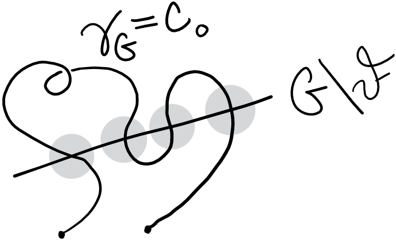
Figure 5. The path $\gamma_{G}$ in $G$, with neighborhoods of its intersection with $G\setminus\mathscr{F}$ highlighted in gray

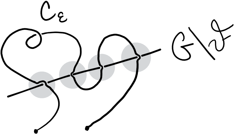
Figure 6. A path $c_{\varepsilon}$ in $G$, which satisfies $c_{\varepsilon}([0,1])\subseteq\mathscr{F}$ and coincides with $\gamma_{G}=c_{0}$ outside of the highlighted neighborhoods of the intersections of $\gamma_{G}$ with $G\setminus\mathscr{F}$

Recall that, because $\operatorname{\mathrm{Hol}}_{\psi(e)}(\mathscr{G},\omega)=\{e\}$, we obtain a well-defined geometric map $\delta:(\mathscr{G},\omega)\to(G,\omega_{{}_{G}})$ given by $\gamma(1)h\mapsto\gamma_{G}(1)h$ for every $h\in H$ and piecewise smooth path $\gamma:[0,1]\to\mathscr{G}$ starting at $\gamma(0)=\psi(e)$. By definition, then, we have that $\delta(\gamma)=\gamma_{G}$ whenever $\gamma(0)=\psi(e)$, so $(\delta\circ\psi)(\gamma_{G})=\gamma_{G}$ whenever $\gamma_{G}$ is contained in $\mathscr{F}$, hence $\delta\circ\psi$ is the identity map on $\mathscr{F}$.

It just remains to show that $\delta$ is a geometric embedding. To this end, suppose $\delta(\mathscr{g})\in\mathscr{F}$, and let $\gamma:[0,1]\to\mathscr{G}$ be a path with $\gamma(0)=\psi(e)$ and $\gamma(1)\in\mathscr{g}H$. Then, $\delta(\gamma)$ is a path in $G$ with $\delta(\gamma(0))=e$ and $\delta(\gamma(1))\in\delta(\mathscr{g})H$. Since $G\setminus\mathscr{F}$ has codimension at least two, we get another homotopy $c:[0,1]^{2}\to G$ such that $c((0,1]\times[0,1])\subseteq\mathscr{F}$ and $c_{s}(t)=c_{0}(t)$ for all $s\in[0,1]$ and $t$ outside small intervals on which $c_{0}=\delta(\gamma)$ intersects $G\setminus\mathscr{F}$. For each $s\in(0,1]$, $\psi(c_{s})$ is well-defined with $\psi(c_{s})_{G}=c_{s}$, so since $\psi(c_{s}(1))$ is constant in $s$, it must be equal to $\gamma(1)$. In particular, $\gamma(1)\in\psi(\mathscr{F})$, so $\mathscr{g}\in\psi(\mathscr{F})$, hence $\delta^{-1}(\mathscr{F})=\psi(\mathscr{F})$. Finally, because $\delta\circ\psi=\mathrm{id}_{\mathscr{F}}$, the restriction $\delta|_{\psi(\mathscr{F})}$ is injective, so $\delta$ is injective by Lemma 5.6.∎

To summarize, we have shown that, if $a\in H$ is flamboyant for $(G,H)$ and $\alpha\in\operatorname{\mathrm{Aut}}(\mathscr{G},\omega)$ with isotropy $a$ at some $\mathscr{e}\in\mathscr{G}$ such that the curvature of $(\mathscr{G},\omega)$ vanishes in some neighborhood of $\mathscr{e}$, then there is a geometric embedding $\delta:(\mathscr{G},\omega)\hookrightarrow(G,\omega_{{}_{G}})$ into the Klein geometry of type $(G,H)$ whose image is the dense open subset given by the image of the sprawl generated by $a$. Thus, we have proven Theorem 5.5.

Now, to prove Theorems A, B, and C, we just need to prove that the relevant isotropies $a\in P_{+}$ are flamboyant, since the results from Section 3 guarantee that the curvature vanishes in a neighborhood of a higher-order fixed point with isotropy $a$.

5.2. Proof of Theorem A

Recall that, in this case, our model is $(\operatorname{\mathrm{PGL}}_{m+1}\mathbb{C},P)$, which corresponds to complex projective geometry over $\mathbb{CP}^{m}$. Proposition 3.2 tells us that the curvature vanishes in a neighborhood of $\mathscr{e}\in\mathscr{G}$, and using the same block sizes as in the proof of that proposition, we may assume that

$$a=\begin{pmatrix}1&1&0\\ 0&1&0\\ 0&0&\mathds{1}\end{pmatrix}$$

after conjugating by an element of $P$. Using Theorem 5.5, it just remains to show that $a$ is flamboyant for $(\operatorname{\mathrm{PGL}}_{m+1}\mathbb{C},P)$.

For arbitrary

$$q_{{}_{P}}(g):=\begin{pmatrix}r\\ x\\ y\end{pmatrix}\in\mathbb{CP}^{m},$$

with $r,x\in\mathbb{C}$ and $y\in\mathbb{C}^{m-1}$, we have

$$a^{k}(q_{{}_{P}}(g))=a^{k}\begin{pmatrix}r\\ x\\ y\end{pmatrix}=\begin{pmatrix}1&k&0\\ 0&1&0\\ 0&0&\mathds{1}\end{pmatrix}\begin{pmatrix}r\\ x\\ y\end{pmatrix}=\begin{pmatrix}r+kx\\ x\\ y\end{pmatrix},$$

which is equal to

$$\begin{pmatrix}1\\ \frac{x}{r+kx}\\ \frac{1}{r+kx}y\end{pmatrix}$$

whenever $r+kx\neq 0$. In particular, fixed points are precisely those points for which $x=0$, and if $x\neq 0$, then $a^{k}(q_{{}_{P}}(g))$ must go to $q_{{}_{P}}(e)$ as $k\rightarrow+\infty$. Since $x=0$ implies $\mathrm{Re}(x)=0$ and $\mathrm{Im}(x)=0$, the set $\mathrm{Fix}_{\mathbb{CP}^{m}}(a)$ of all points for which $x=0$ is of codimension 2.

Now, all that is left to do is construct a flamboyance for $a$. Because $a$ is a complex projective automorphism, it always sends complex lines to complex lines, and since $a$ has a higher-order fixed point at $q_{{}_{P}}(e)$, it specifically preserves each complex line through $q_{{}_{P}}(e)$. Let $\mathcal{L}$ be the set of all complex lines $\ell$ such that $\ell\cap\mathrm{Fix}_{\mathbb{CP}^{m}}(a)=\{q_{{}_{P}}(e)\}$. Each of these complex lines $\ell$ is $a$-invariant, and since $\ell\cong\mathbb{CP}^{1}$, they are all compact and simply connected. Moreover, whenever $q_{{}_{P}}(g)\neq q_{{}_{P}}(e)$, there is a unique complex line containing both $q_{{}_{P}}(g)$ and $q_{{}_{P}}(e)$, so the intersection of different elements of $\mathcal{L}$ is always the path-connected subset $\{q_{{}_{P}}(e)\}$ and each non-fixed point of $\mathbb{CP}^{m}$ is contained in some element of $\mathcal{L}$. Thus, $\mathcal{L}$ is a flamboyance for $a$, which completes the proof of Theorem A.

5.3. Proof of Theorem B

This proof is largely the same as the one for Theorem A. In this case, the model becomes $(\operatorname{\mathrm{PGL}}_{m+1}\mathbb{H},P)$, with $\operatorname{\mathrm{PGL}}_{m+1}\mathbb{H}/P\cong\mathbb{HP}^{m}$. After conjugating by an element of $P$, we may assume that

$$a=\begin{pmatrix}1&1&0\\ 0&1&0\\ 0&0&\mathds{1}\end{pmatrix},$$

and by Theorem 5.4 of [11], the curvature vanishes in a neighborhood of $\mathscr{e}$. Now, we just need to show $a$ is flamboyant.

For arbitrary

$$q_{{}_{P}}(g):=\begin{pmatrix}r\\ x\\ y\end{pmatrix}\in\mathbb{HP}^{m},$$

with $r,x\in\mathbb{H}$ and $y\in\mathbb{H}^{m-1}$, we have

$$a^{k}(q_{{}_{P}}(g))=a^{k}\begin{pmatrix}r\\ x\\ y\end{pmatrix}=\begin{pmatrix}1&k&0\\ 0&1&0\\ 0&0&\mathds{1}\end{pmatrix}\begin{pmatrix}r\\ x\\ y\end{pmatrix}=\begin{pmatrix}r+kx\\ x\\ y\end{pmatrix},$$

which is equal to

$$\begin{pmatrix}1\\ x(r+kx)^{-1}\\ y(r+kx)^{-1}\end{pmatrix}$$

whenever $r+kx\neq 0$. In particular, fixed points are precisely those points for which $x=0$, and if $x\neq 0$, then $a^{k}(q_{{}_{P}}(g))$ must go to $q_{{}_{P}}(e)$ as $k\rightarrow+\infty$. This time, the set $\mathrm{Fix}_{\mathbb{HP}^{m}}(a)$ of all points for which $x=0$ is of codimension $\dim(\mathbb{H})=4$.

We again end the proof by finding a flamboyance for $a$. Because $a$ is a quaternionic projective automorphism, it sends quaternionic lines to quaternionic lines, and since $a$ has a higher-order fixed point at $q_{{}_{P}}(e)$, it specifically preserves each quaternionic line through $q_{{}_{P}}(e)$. Therefore, we can let $\mathcal{L}$ be the set of all quaternionic lines $\ell$ such that $\ell\cap\mathrm{Fix}_{\mathbb{HP}^{m}}(a)=\{q_{{}_{P}}(e)\}$. Each of these quaternionic lines $\ell\cong\mathbb{HP}^{1}$ is $a$-invariant, simply connected, and compact. Moreover, whenever $q_{{}_{P}}(g)\neq q_{{}_{P}}(e)$, there is a unique quaternionic line containing both $q_{{}_{P}}(g)$ and $q_{{}_{P}}(e)$, so each non-fixed point of $\mathbb{HP}^{m}$ is contained in some element of $\mathcal{L}$ and the intersection of different elements of $\mathcal{L}$ is always the path-connected subset $\{q_{{}_{P}}(e)\}$. Thus, $\mathcal{L}$ is a flamboyance for $a$, which completes the proof of Theorem B.

5.4. Proof of Theorem C

For this theorem, our model is given by $(\operatorname{\mathrm{PU}}(\mathrm{h}_{p,q}),P)$, corresponding to the natural partially integrable almost CR-structure on the null-cone for $\mathrm{h}_{p,q}$ in $\mathbb{CP}^{p+q+1}$. This time, there are essentially three different possibilities for $a$ up to conjugation by an element of $P$: $a\in\exp(\mathfrak{g}_{1})$ “timelike”, $a\in\exp(\mathfrak{g}_{1})$ “spacelike”, or $a\in\exp(\mathfrak{g}_{2})=\mathrm{Z}(P_{+})$. Since the “timelike” and “spacelike” cases are mostly the same, we will just treat the “timelike” case. Therefore, after conjugation by an element of $P$ and possibly considering $\alpha^{-1}$ instead of $\alpha$, we can assume that either

$$a=\begin{pmatrix}1&0&0&\mathrm{i}\\ 0&1&0&0\\ 0&0&\mathds{1}&0\\ 0&0&0&1\end{pmatrix}\in\mathrm{Z}(P_{+})$$

or

$$a=\begin{pmatrix}1&1&0&-1/2\\ 0&1&0&-1\\ 0&0&\mathds{1}&0\\ 0&0&0&1\end{pmatrix}\in\exp(\mathfrak{g}_{1}),$$

where for convenience we use the same block sizes as in the proof of Proposition 3.7 throughout. In either case, we get a flat neighborhood of $\mathscr{e}$, by Theorem 3.9 of [3] for $a\in\mathrm{Z}(P_{+})$ and by Proposition 3.7 of this paper for non-null $a\in\exp(\mathfrak{g}_{1})$, so we just need to show that $a$ is flamboyant.

Let us do the $a\in\mathrm{Z}(P_{+})$ case first. For an arbitrary element

$$q_{{}_{P}}(g):=\begin{pmatrix}r\\ x\\ y\\ c\end{pmatrix}\in\mathrm{Null}(\mathrm{h}_{p,q})\subseteq\mathbb{CP}^{p+q+1}$$

of the null-cone for $\mathrm{h}_{p,q}$, so that $r,x,c\in\mathbb{C}$ and $y\in\mathbb{C}^{p+q-1}$ satisfy $2\mathrm{Re}(\bar{r}c)+|x|^{2}+\bar{y}^{\top}I_{p-1,q}y=0$, we can use our chosen representative for $a\in\mathrm{Z}(P_{+})$ to get

$$a^{k}(q_{{}_{P}}(g))=a^{k}\begin{pmatrix}r\\ x\\ y\\ c\end{pmatrix}=\begin{pmatrix}1&0&0&k\mathrm{i}\\ 0&1&0&0\\ 0&0&\mathds{1}&0\\ 0&0&0&1\end{pmatrix}\begin{pmatrix}r\\ x\\ y\\ c\end{pmatrix}=\begin{pmatrix}r+kc\mathrm{i}\\ x\\ y\\ c\end{pmatrix},$$

which is equal to

$$\begin{pmatrix}1\\ \frac{x}{r+kc\mathrm{i}}\\ \frac{y}{r+kc\mathrm{i}}\\ \frac{c}{r+kc\mathrm{i}}\end{pmatrix}$$

whenever $r+kc\mathrm{i}\neq 0$. In particular, the set of fixed points for $a$ is precisely the set of points for which $c=0$, and whenever $c\neq 0$, $a^{k}(q_{{}_{P}}(g))$ must go to $q_{{}_{P}}(e)$ as $k\rightarrow+\infty$. The set $\mathrm{Fix}_{G/P}(a)$ of all points in $\mathrm{Null}(\mathrm{h}_{p,q})$ with $c=0$ is of codimension 2; note that, if $c=0$, then in order to stay in the null-cone, we must also have $|x|^{2}+\bar{y}^{\top}I_{p-1,q}y=0$.

Now, we construct a flamboyance for the isotropy $a\in\mathrm{Z}(P_{+})$. For each $(\begin{smallmatrix}x\\ y\end{smallmatrix})\in\mathbb{CP}^{p+q-1}$, with $x\in\mathbb{C}$ and $y\in\mathbb{C}^{p+q-1}$, consider the subspace

$$\ell_{x,y}:=\left\{\begin{pmatrix}r\\ zx\\ zy\\ c\end{pmatrix}\in\mathrm{Null}(\mathrm{h}_{p,q}):r,c,z\in\mathbb{C}\right\}.$$

Each of these subspaces $\ell_{x,y}$ is preserved by $a$, and if $|x|^{2}+\bar{y}^{\top}I_{p-1,q}y\neq 0$, then the only fixed point of $a$ in $\ell_{x,y}$ is $q_{{}_{P}}(e)$. Moreover, $\ell_{x,y}$ is a copy of $\mathrm{Null}(\mathrm{h}_{1,0})$ if $|x|^{2}+\bar{y}^{\top}I_{p-1,q}y>0$ and a copy of $\mathrm{Null}(\mathrm{h}_{0,1})$ if $|x|^{2}+\bar{y}^{\top}I_{p-1,q}y<0$; either way, $\ell_{x,y}$ is diffeomorphic to $S^{3}$, hence compact and simply connected. Thus, we let

$$\mathcal{L}:=\{\ell_{x,y}:|x|^{2}+\bar{y}^{\top}I_{p-1,q}y\neq 0\}.$$

For $(\begin{smallmatrix}x\\ y\end{smallmatrix})\neq(\begin{smallmatrix}x^{\prime}\\ y^{\prime}\end{smallmatrix})\in\mathbb{CP}^{p+q-1}$,

$$\ell_{x,y}\cap\ell_{x^{\prime},y^{\prime}}=\left\{\begin{pmatrix}r\\ 0\\ 0\\ c\end{pmatrix}\in\mathrm{Null}(\mathrm{h}_{p,q}):r,c\in\mathbb{C}\right\}\cong\mathbb{RP}^{1},$$

which is path-connected, and

$$\begin{pmatrix}r\\ x\\ y\\ c\end{pmatrix}\in\ell_{x,y},$$

so every non-fixed point is contained in some $\ell_{x,y}\in\mathcal{L}$. In other words, $\mathcal{L}$ is a flamboyance for $a\in\mathrm{Z}(P_{+})$, hence $a$ is flamboyant in that case.

It remains to prove that non-null $a\in\exp(\mathfrak{g}_{1})$ are flamboyant. This time, using our chosen representative for $a\in\exp(\mathfrak{g}_{1})$, we get

$$a^{k}(q_{{}_{P}}(g))=a^{k}\begin{pmatrix}r\\ x\\ y\\ c\end{pmatrix}=\begin{pmatrix}1&k&0&-k^{2}/2\\ 0&1&0&-k\\ 0&0&\mathds{1}&0\\ 0&0&0&1\end{pmatrix}\begin{pmatrix}r\\ x\\ y\\ c\end{pmatrix}=\begin{pmatrix}r+kx-\frac{k^{2}c}{2}\\ x-kc\\ y\\ c\end{pmatrix}.$$

The expression $r+kx-k^{2}\frac{c}{2}$ grows quadratically in $k$ if $c\neq 0$, linearly in $k$ if $c=0$ but $x\neq 0$, and is constant if $x=c=0$, while $x-kc$ grows linearly in $k$ if $c\neq 0$ and is constant if $c=0$. In particular, $a^{k}(q_{{}_{P}}(g))$ must converge to $q_{{}_{P}}(e)$ as $k\rightarrow+\infty$ unless $x=c=0$. The points with $x=c=0$ are the fixed points of $a$, so this time $\mathrm{Fix}_{G/P}(a)$ has codimension $2+2=4$. Note that, in order to stay inside of the null-cone, if $x=c=0$, then we must also have $\bar{y}^{\top}I_{p-1,q}y=0$.

To construct a flamboyance for $a\in\exp(\mathfrak{g}_{1})$, we consider subspaces of the form

$$\ell_{y}:=\left\{\begin{pmatrix}r\\ x\\ zy\\ c\end{pmatrix}\in\mathrm{Null}(\mathrm{h}_{p,q}):r,x,c,z\in\mathbb{C}\right\}$$

for each $y\in\mathbb{C}^{p+q-1}$. These are each preserved by $a$, and whenever $\bar{y}^{\top}I_{p-1,q}y\neq 0$, the only fixed point contained in $\ell_{y}$ is $q_{{}_{P}}(e)$. Moreover, $\ell_{y}$ is a copy of $\mathrm{Null}(\mathrm{h}_{2,0})$ if $\bar{y}^{\top}I_{p-1,q}y>0$ and a copy of $\mathrm{Null}(\mathrm{h}_{1,1})$ if $\bar{y}^{\top}I_{p-1,q}y<0$; either way, $\ell_{y}$ is simply connected and compact. Thus, we let

$$\mathcal{L}:=\{\ell_{y}:\bar{y}^{\top}I_{p-1,q}y\neq 0\}.$$

For linearly independent $y$ and $y^{\prime}$ in $\mathbb{C}^{p+q-1}$,

$$\ell_{y}\cap\ell_{y^{\prime}}=\left\{\begin{pmatrix}r\\ x\\ 0\\ c\end{pmatrix}\in\mathrm{Null}(\mathrm{h}_{p,q}):r,x,c\in\mathbb{C}\right\}\cong\mathrm{Null}(\mathrm{h}_{1,0}),$$

which is path-connected, and

$$\begin{pmatrix}r\\ x\\ y\\ c\end{pmatrix}\in\ell_{y},$$

so every non-fixed point is contained in some $\ell_{y}\in\mathcal{L}$. By definition, this means $\mathcal{L}$ is a flamboyance for $a\in\exp(\mathfrak{g}_{1})$, hence $a$ is flamboyant in this case as well. This completes the proof of Theorem C.

Appendix: the holonomy group of the sprawl

In anticipation of a growing interest in techniques revolving around the holonomy group of a Cartan geometry, we have decided to include the following supplementary result. Throughout the proof, we will unabashedly use the ideas from [5] on developments of points and their relations to automorphisms.

Proposition 5.10.

For $(\mathscr{F},\sigma^{*}\omega)$ the sprawl of $(q_{{}_{H}}^{-1}(U),\omega)$ generated by $\alpha\in\operatorname{\mathrm{Aut}}(\mathscr{G},\omega)$ from $\mathscr{e}$, let $a\in G$ be a development of $\alpha(\mathscr{e})$ from $\mathscr{e}$ as elements of $(q_{{}_{H}}^{-1}(U),\omega)$. The holonomy group $\operatorname{\mathrm{Hol}}_{\mathscr{e}}(\mathscr{F},\sigma^{*}\omega)$ of the sprawl is the smallest subgroup of $G$ containing $\operatorname{\mathrm{Hol}}_{\mathscr{e}}(q_{{}_{H}}^{-1}(U),\omega)$ that is normalized by $a$.

Proof.

Suppose $\gamma:[0,1]\to\mathscr{F}$ is a path lying over a loop $q_{{}_{H}}(\gamma)$ in $q_{{}_{H}}(\mathscr{F})$, with $\gamma(0)=\mathscr{e}$ and $\gamma(1)=\gamma(0)h_{\gamma}$. We want to compute $\gamma_{G}(1)h_{\gamma}^{-1}$. First, we will show that we can assume $\gamma$ lies over a loop incremented from $0$ to $0$, and then we will compute what $\gamma_{G}(1)h_{\gamma}^{-1}$ can be.

Let us break $\gamma$ into a concatenation of segments $\gamma=\gamma_{0}\star\cdots\star\gamma_{\ell-1}$ such that, for each $0\leq j<\ell$, $\gamma_{j}([0,1])\subseteq\tilde{\alpha}^{k_{j}}(q_{{}_{H}}^{-1}(U))$ for some $k_{j}\in\mathbb{Z}$. By definition of sprawl-equivalence, for

$$\gamma_{j}(1)=\gamma_{j+1}(0)\in\tilde{\alpha}^{k_{j}}(q_{{}_{H}}^{-1}(U))\cap\tilde{\alpha}^{k_{j+1}}(q_{{}_{H}}^{-1}(U)),$$

there must be a thinly null-homotopic loop $\gamma_{j,j+1}$ based at $\gamma_{j}(1)$ with $q_{{}_{H}}(\gamma_{j,j+1})$ incremented from $k_{j}$ to $k_{j+1}$. In particular, the modified path

$$\gamma_{0}\star\gamma_{0,1}\star\gamma_{1}\star\gamma_{1,2}\star\cdots\star\gamma_{\ell-1}\star\gamma_{\ell-1,\ell}\star\gamma_{\ell}$$

in $\mathscr{F}$ descends to a loop in $q_{{}_{H}}(\mathscr{F})$ with an incrementation from $0$ to $k_{\ell}$, and since the holonomy of a thinly null-homotopic loop is always trivial,

$$(\gamma_{0}\star\gamma_{0,1}\star\gamma_{1}\star\gamma_{1,2}\star\cdots\star\gamma_{\ell-1}\star\gamma_{\ell-1,\ell}\star\gamma_{\ell})_{G}(1)=\gamma_{G}(1).$$

Thus, without loss of generality, we may assume that $\gamma$ lies over a loop $q_{{}_{H}}(\gamma)$ that is incremented from $0$ to $k_{\ell}$ for some $k_{\ell}\in\mathbb{Z}$. Moreover, since

$$q_{{}_{H}}(\mathscr{e})=q_{{}_{H}}(\gamma(0))=q_{{}_{H}}(\gamma(1))\in\tilde{\alpha}^{0}(U)\cap\tilde{\alpha}^{k_{\ell}}(U),$$

there must be a thinly null-homotopic loop $\gamma^{\prime}$ based $\mathscr{e}$ such that $q_{{}_{H}}(\gamma^{\prime})$ is incremented from $0$ to $k_{\ell}$. Concatenating $\gamma$ with $\operatorname{R}_{h_{\gamma}}(\overline{\gamma^{\prime}})$, we again get a path $\gamma\star\operatorname{R}_{h_{\gamma}}(\overline{\gamma^{\prime}})$ lying over a loop in $q_{{}_{H}}(\mathscr{F})$, this time with an incrementation from $0$ to $0$, such that $(\gamma\star\operatorname{R}_{h_{\gamma}}(\overline{\gamma^{\prime}}))_{G}(1)=\gamma_{G}(1)$. Without loss of generality, we may therefore assume that $\gamma$ lies over a loop $q_{{}_{H}}(\gamma)$ with an incrementation from $0$ back to $0$.

Let this incrementation of the loop $q_{{}_{H}}(\gamma)$ from $0$ to $0$ be given by the partition $0=t_{0}<\cdots<t_{\ell}=1$ and the finite integer sequence $k_{0}=0,\dots,k_{\ell-1}=0\in\mathbb{Z}$. By definition, $\gamma(t_{j+1})$ lies over the connected component of $\tilde{\alpha}^{k_{j}}(U)\cap\tilde{\alpha}^{k_{j+1}}(U)$ containing $q_{{}_{H}}(\tilde{\alpha}^{\max(k_{j},k_{j+1})}(\mathscr{e}))$, so there exist paths

$$\beta_{j+1}:[0,1]\to\tilde{\alpha}^{k_{j}}(q_{{}_{H}}^{-1}(U))\cap\tilde{\alpha}^{k_{j+1}}(q_{{}_{H}}^{-1}(U))$$

with $\beta_{j+1}(0)=\gamma(t_{j+1})$ and $\beta_{j+1}(1)b_{j+1}=\tilde{\alpha}^{\max(k_{j},k_{j+1})}(\mathscr{e})$ for some $b_{j+1}\in H$. In particular, $\beta_{j+1}\star\overline{\beta_{j+1}}$ is a thinly null-homotopic loop in $\tilde{\alpha}^{k_{j}}(q_{{}_{H}}^{-1}(U))\cap\tilde{\alpha}^{k_{j+1}}(q_{{}_{H}}^{-1}(U))$, so we may again construct a modified path

$$\gamma|_{[0,t_{1}]}\star\beta_{1}\star\overline{\beta_{1}}\star\cdots\star\gamma|_{[t_{\ell-2},t_{\ell-1}]}\star\beta_{\ell-1}\star\overline{\beta_{\ell-1}}\star\gamma|_{[t_{\ell-1},1]}$$

with the same total development as $\gamma$; this tells us that we may further assume, without loss of generality, that $\gamma(t_{j+1})b_{j+1}=\alpha^{\max(k_{j},k_{j+1})}(\mathscr{e})$ for some $b_{j+1}\in H$ for each $0\leq j<\ell-1$.

With this, each segment $\gamma|_{[t_{j},t_{j+1}]}$ with $0\leq j<\ell-1$ is a path from $\gamma(t_{j})=\tilde{\alpha}^{\max(k_{j-1},k_{j})}(\mathscr{e})b_{j}^{-1}$ to $\gamma(t_{j+1})=\tilde{\alpha}^{\max(k_{j},k_{j+1})}(\mathscr{e})b_{j+1}^{-1}$, so since the space of possible developments from $\tilde{\alpha}^{\max(k_{j-1},k_{j})}(\mathscr{e})$ to $\tilde{\alpha}^{\max(k_{j},k_{j+1})}(\mathscr{e})$ is just

$$\operatorname{\mathrm{Hol}}_{\mathscr{e}}(q_{{}_{H}}^{-1}(U),\omega)a^{\max(k_{j},k_{j+1})-\max(k_{j-1},k_{j})}=\operatorname{\mathrm{Hol}}_{\mathscr{e}}(q_{{}_{H}}^{-1}(U),\omega)a^{\frac{1}{2}(k_{j+1}-k_{j-1})},$$

we must have

$$(\gamma|_{[t_{j},t_{j+1}]})_{G}(t_{j+1})=b_{j}\eta_{j}a^{\frac{1}{2}(k_{j+1}-k_{j-1})}b_{j+1}^{-1}$$

for some $\eta_{j}\in\operatorname{\mathrm{Hol}}_{\mathscr{e}}(q_{{}_{H}}^{-1}(U),\omega)$. Crucially, note that for another path $\zeta:[0,1]\to q_{{}_{H}}^{-1}(U)$ with $\zeta(0)=\mathscr{e}$ and $\zeta(1)=\zeta(0)h_{\zeta}=\mathscr{e}h_{\zeta}$, we can replace $\gamma|_{[t_{j},t_{j+1}]}$ with $\tilde{\alpha}^{\max(k_{j-1},k_{j})}(\operatorname{R}_{b_{j}^{-1}}(\zeta))\star\operatorname{R}_{b_{j}h_{\zeta}b_{j}^{-1}}(\gamma|_{[t_{j},t_{j+1}]})$ to change the total development of $\gamma|_{[t_{j},t_{j+1}]}$ from $b_{j}\eta_{j}a^{\frac{1}{2}(k_{j+1}-k_{j-1})}b_{j+1}^{-1}$ to

$$(b_{j}\zeta_{G}(1)b_{j}^{-1})(b_{j}h_{\zeta}^{-1}b_{j}^{-1})(b_{j}\eta_{j}a^{\frac{1}{2}(k_{j+1}-k_{j-1})}b_{j+1}^{-1})(b_{j}h_{\zeta}b_{j}^{-1}),$$

which is just $b_{j}(\zeta_{G}(1)h_{\zeta}^{-1})\eta_{j}a^{\frac{1}{2}(k_{j+1}-k_{j-1})}(b_{j}h_{\zeta}b_{j}^{-1}b_{j+1})^{-1}$, so replacing $b_{j+1}$ with $b_{j}h_{\zeta}b_{j}^{-1}b_{j+1}$, every $\eta_{j}\in\operatorname{\mathrm{Hol}}_{\mathscr{e}}(q_{{}_{H}}^{-1}(U),\omega)$ can be realized in the total development $b_{j}\eta_{j}a^{\frac{1}{2}(k_{j+1}-k_{j-1})}b_{j+1}^{-1}$ of the segment $\gamma|_{[t_{j},t_{j+1}]}$ for some $\gamma$ with the given incrementation from $0$ to $0$.

Similarly, for the final segment $\gamma|_{[t_{\ell-1},1]}$ of $\gamma$, we get a path from $\gamma(t_{\ell-1})=\tilde{\alpha}^{\max(k_{\ell-2},k_{\ell-1})}(\mathscr{e})b_{\ell-1}^{-1}$ to $\gamma(1)=\gamma(0)h_{\gamma}=\mathscr{e}h_{\gamma}$, so

$$(\gamma|_{[t_{\ell-1},1]})_{G}(1)=b_{\ell-1}\eta_{\ell-1}a^{-\max(k_{\ell-2},k_{\ell-1})}h_{\gamma}$$

for some $\eta_{\ell-1}\in\operatorname{\mathrm{Hol}}_{\mathscr{e}}(q_{{}_{H}}^{-1}(U),\omega)$. Again, by modifying the segment and $h_{\gamma}$, we can realize any $\eta_{\ell-1}\in\operatorname{\mathrm{Hol}}_{\mathscr{e}}(q_{{}_{H}}^{-1}(U),\omega)$ in this total development of the segment.

Putting all of this together,

$$\gamma_{G}(1) =(\gamma|_{[0,t_{1}]})_{G}(t_{1})\cdots(\gamma|_{[t_{\ell-1},1]})_{G}(1)$$

$$=(\eta_{0}a^{k_{1}}b_{1}^{-1})(b_{1}\eta_{1}a^{\frac{1}{2}(k_{2}-k_{0})}b_{2}^{-1})\cdots(b_{\ell-1}\eta_{\ell-1}a^{-\max(k_{\ell-2},k_{\ell-1})}h_{\gamma})$$

$$=\eta_{0}a^{k_{1}}\eta_{1}a^{\frac{1}{2}(k_{2}-k_{0})}\cdots\eta_{\ell-1}a^{-\max(k_{\ell-2},k_{\ell-1})}h_{\gamma},$$

so

$$\gamma_{G}(1)h_{\gamma}^{-1}=\eta_{0}a^{k_{1}}\eta_{1}a^{\frac{1}{2}(k_{2}-k_{0})}\cdots\eta_{\ell-1}a^{-\max(k_{\ell-2},k_{\ell-1})}.$$

Note, though, that because the labels $k_{j}$ come from an incrementation, each of the powers of $a$ in this expression is either $a^{-1}$, $a^{0}=e$, or $a^{1}=a$, with the sum of the first $j$ powers of $a$ precisely equal to $k_{j}$. Moreover, since the incrementation is from $0$ to $0$, the elements $a$ and $a^{-1}$ must occur in pairs, so that $\gamma_{G}(1)h_{\gamma}^{-1}$ is in the smallest subgroup containing $\operatorname{\mathrm{Hol}}_{\mathscr{e}}(q_{{}_{H}}^{-1}(U),\omega)$ closed under conjugation by powers of $a$. Thus, $\gamma_{G}(1)h_{\gamma}^{-1}$ is contained in the desired subgroup. Finally, because every $\eta_{j}\in\operatorname{\mathrm{Hol}}_{\mathscr{e}}(q_{{}_{H}}^{-1}(U),\omega)$ can be realized in the above expression for some $\gamma$ with the given incrementation, we can get every element of the desired subgroup by considering paths $\gamma$ with different incrementations from $0$ to $0$, hence $\operatorname{\mathrm{Hol}}_{\mathscr{e}}(\mathscr{F},\sigma^{*}\omega)$ is equal to this subgroup.∎

References

- [1] Caetano, A., Picken, R. F.: An axiomatic definition of holonomy. International Journal of Mathematics, vol. 5, no. 6, 835-848 (1994)
- [2] Calderbank, D. M. J., et al.: C-projective geometry. Memoirs of the American Mathematical Society, vol. 267, no. 1299 (2020)
- [3] Čap, A., Melnick, K.: Essential Killing fields of parabolic geometries. Indiana University Mathematics Journal, vol. 62, no. 6, 1917-1953 (2013)
- [4] Čap, A., Slovák, J.: Parabolic Geometries I: Background and General Theory. Mathematical Surveys and Monographs, vol. 154. Amer. Math. Soc., Providence, RI (2009)
- [5] Erickson, J. W.: Intrinsic holonomy and curved cosets of Cartan geometries. European Journal of Mathematics, vol. 8, 446-474 (2022)
- [6] Frances, C.: Sur le groupe d’automorphismes des géomètries paraboliques de rang un. Annales scientifiques de l’Ecole Normale Supérieure, vol. 40 (2007) [English version available at https://irma.math.unistra.fr/~frances/cartan-english6.pdf , accessed January 25, 2023]
- [7] Frances, C., Melnick, K.: The Lorentzian Lichnerowicz Conjecture for real-analytic, three-dimensional manifolds. arXiv:2108.07215v1
- [8] Kruglikov, B., The, D.: Jet-determination of symmetries of parabolic geometries. Mathematische Annalen, vol. 371, 1575-1613 (2018)
- [9] Ma, T.: Geodesic rigidity of Levi-Civita connections admitting essential projective vector fields. Geom Dedicata, vol. 205, 147-166 (2020)
- [10] Melnick, K.: Rigidity of transformation groups in differential geometry. Notices of the American Mathematical Society, vol. 68, no. 5, 721-732 (2021)
- [11] Melnick, K., Neusser, K.: Strongly essential flows on irreducible parabolic geometries. Transactions of the American Mathematical Society, vol. 368, no. 11, 8079-8110 (2016)
- [12] Melnick, K., Pecastaing, V.: The conformal group of a compact, simply connected Lorentzian manifold. Journal of the American Mathematical Society, vol. 35, no. 1, 81-122 (2022)
- [13] Sharpe, R. W.: Differential Geometry: Cartan’s Generalization of Klein’s Erlangen Program. Graduate Texts in Mathematics, vol. 166, Springer-Verlag, New York (1997)