Toward minimal composite Higgs models from
regular geometries in bottom-up holography

Abstract

We study a bottom-up, holographic description of a field theory yielding the spontaneous breaking of an approximate $SO(5)$ global symmetry to its $SO(4)$ subgroup. The weakly-coupled, six-dimensional gravity dual has regular geometry. One of the dimensions is compactified on a circle that shrinks smoothly to zero size at a finite value of the holographic direction, hence introducing a physical scale in a way that mimics the effect of confinement in the dual four-dimensional field theory. We study the spectrum of small fluctuations of the bulk fields carrying $SO(5)$ quantum numbers, which can be interpreted as spin-0 and spin-1 bound states in the dual field theory. This work supplements an earlier publication, focused only on the $SO(5)$ singlet states. We explore the parameter space of the theory, paying particular attention to composite states that have the right quantum numbers to be identified as pseudo-Nambu-Goldstone Bosons (PNGBs).

We find that in this model the PNGBs are generally heavy, with masses of the same order as other bound states, indicating the presence of a sizeable amount of explicit symmetry breaking in the field theory side. But we also find a qualitatively new, unexpected result. When the dimension of the field-theory operator inducing $SO(5)$ breaking is close to half of the space-time dimensionality, there exists a region of parameter space in which the PNGBs and the lightest scalar are both parametrically light in comparison to all other bound states of the field theory. Although this region is known to yield metastable classical backgrounds, this finding might be relevant to model building in the composite Higgs context.

I Introduction

It has been just over ten years since the discovery of the Higgs boson Aad:2012tfa ; Chatrchyan:2012xdj , and in the intervening time composite Higgs models (CHMs) Kaplan:1983fs ; Georgi:1984af ; Dugan:1984hq , in which the Higgs fields originate as composite, pseudo-Nambu-Goldstone bosons (PNGBs) in a more fundamental theory, have gained much attention in the literature—see Refs. Panico:2015jxa ; Witzel:2019jbe ; Cacciapaglia:2020kgq , and the summary tables in Refs. Ferretti:2013kya ; Ferretti:2016upr ; Cacciapaglia:2019bqz . Phenomenological and model-building studies of realisations of this idea Katz:2005au ; Barbieri:2007bh ; Lodone:2008yy ; Gripaios:2009pe ; Mrazek:2011iu ; Marzocca:2012zn ; Grojean:2013qca ; Barnard:2013zea ; Cacciapaglia:2014uja ; Ferretti:2014qta ; Arbey:2015exa ; vonGersdorff:2015fta ; Vecchi:2015fma ; Cacciapaglia:2015eqa ; Ma:2015gra ; Feruglio:2016zvt ; DeGrand:2016pgq ; Fichet:2016xvs ; Galloway:2016fuo ; Agugliaro:2016clv ; Belyaev:2016ftv ; Bizot:2016zyu ; Csaki:2017cep ; Chala:2017sjk ; Golterman:2017vdj ; Csaki:2017jby ; Alanne:2017rrs ; Alanne:2017ymh ; Sannino:2017utc ; Alanne:2018wtp ; Bizot:2018tds ; Cai:2018tet ; Agugliaro:2018vsu ; BuarqueFranzosi:2018eaj ; Cacciapaglia:2018avr ; Gertov:2019yqo ; Ayyar:2019exp ; Cacciapaglia:2019ixa ; BuarqueFranzosi:2019eee ; Cacciapaglia:2019dsq ; Cacciapaglia:2020vyf ; Banerjee:2022izw ; Appelquist:2020bqj ; Cacciapaglia:2021uqh ; Appelquist:2022qgl ; Ferretti:2022mpy ; Banerjee:2023ipb have been complemented by a growing literature of dedicated lattice calculations, that analyse strongly-coupled field theories providing, at least partial, short-distance completions Hietanen:2014xca ; Detmold:2014kba ; Arthur:2016dir ; Arthur:2016ozw ; Pica:2016zst ; Lee:2017uvl ; Drach:2017btk ; Drach:2020wux ; Drach:2021uhl ; Bennett:2017kga ; Bennett:2019jzz ; Bennett:2019cxd ; Bennett:2022yfa ; Ayyar:2017qdf ; Ayyar:2018zuk ; Ayyar:2018ppa ; Ayyar:2018glg ; Cossu:2019hse ; Shamir:2021frg ; DelDebbio:2021xlv . But providing a compelling microscopic origin for CHMs with minimal $SO(5)/SO(4)$ coset is non-trivial—see for instance Ref. Caracciolo:2012je .

Within string theory and supergravity, it has been discovered that gauge-gravity dualities, or holography Maldacena:1997re ; Gubser:1998bc ; Witten:1998qj ; Aharony:1999ti , provide an alternative way to study special field theories in their non-perturbative regime. Applications include the holographic description of confinement Witten:1998zw ; Klebanov:2000hb ; Maldacena:2000yy ; Butti:2004pk , the study of the composite (glueball) mass spectra Brower:2000rp ; Wen:2004qh ; Kuperstein:2004yf ; Bianchi:2003ug ; Berg:2005pd ; Berg:2006xy ; Elander:2009bm ; Elander:2010wd ; Elander:2013jqa ; Elander:2014ola ; Elander:2017cle ; Elander:2017hyr , chiral symmetry breaking  Karch:2002sh ; Babington:2003vm , and masses of mesons Sakai:2004cn ; Sakai:2005yt ; Kruczenski:2003be ; Nunez:2003cf ; Erdmenger:2007cm . But it is very challenging to embed within string theory and supergravity fully realistic dynamical models yielding the low-energy theories relevant to CHMs. A few steps towards a top-down construction for CHMs with $SO(5)/SO(4)$ coset have been taken recently Elander:2021kxk . A more general, pragmatic, bottom-up approach to holography exists, in which the gravity dual is constructed classically, on the basis of ad hoc simplifying assumptions. Indeed, much work on the minimal $SO(5)/SO(4)$ coset has been developed in this context, and make it a quite compelling scenario Contino:2003ve ; Agashe:2004rs ; Agashe:2005dk ; Agashe:2006at ; Contino:2006qr ; Falkowski:2008fz ; Contino:2010rs ; Contino:2011np . Other CHMs suitable for lattice explorations have been the subject of recent bottom-up holographic studies Erdmenger:2020lvq ; Erdmenger:2020flu ; Elander:2020nyd ; Elander:2021bmt .

In this paper, we outline a new bottom-up holographic realisation of the $SO(5)/SO(4)$ paradigm needed for minimal CHMs. The model is an extended version of the very simple one that was studied in Ref. Elander:2022ebt , admitting the same class of background geometries. While Ref. Elander:2022ebt focuses on identifying regions of parameter space relevant to understanding the physics of the dilaton, the approximate Goldstone boson associated with scale invariance, along the programmatic lines developed in Refs. Kaplan:2009kr ; Gorbenko:2018ncu ; Gorbenko:2018dtm ; Elander:2020ial ; Elander:2020fmv ; Elander:2021wkc , in this publication and in future ones vacuum ; EWSB we are interested in investigating whether the PNGB states associated with the $SO(5)/SO(4)$ coset have model-building potential in the CHM context.

Let us first summarise the salient features of the model, borrowing results from Ref. Elander:2022ebt . A single scalar field is coupled to gravity in six dimensions, and its dynamics is governed by a polynomial potential Goldberger:1999uk ; DeWolfe:1999cp ; Goldberger:1999un ; Csaki:2000zn ; ArkaniHamed:2000ds ; Rattazzi:2000hs ; Kofman:2004tk . A free parameter in the potential determines the dimensionality of the operator (deformation) in the dual five-dimensional field-theory interpretation of the gravity model. Furthermore, one of the space-like dimensions is a circle, its size shrinking along the holographic direction, which introduces a smooth end of space in the regular geometry. As proposed in Ref. Witten:1998zw , in the dual field-theory interpretation this amounts to introducing a mass gap, in a way that mimics what happens for confining theories. Notice that this is the main difference with respect to Refs. Contino:2003ve ; Agashe:2004rs ; Agashe:2005dk ; Agashe:2006at ; Contino:2006qr ; Falkowski:2008fz ; Contino:2010rs ; Contino:2011np , namely the existence of a lift to a completely smooth geometry in six dimensions, which imposes constraints on the bulk profiles of the scalar fields of the five-dimensional gravity theory, obtained after reduction on the circle.

It has been shown in Ref. Elander:2022ebt that a phase transition occurs in the theory. This result was obtained by applying holographic renormalisation Bianchi:2001kw ; Skenderis:2002wp ; Papadimitriou:2004ap to compute the free energy. Whether the regular backgrounds are stable depends on the magnitude of the field-theory deformation. As explained in the body of the paper, the size of such deformation, and its associated condensate, are both extracted from the profile of the bulk fields, but are not independent of one another, as they are constrained by the aforementioned regularity conditions.

The calculation of the spectrum of fluctuations of the bulk fields has a natural holographic interpretation in terms of bound states of the dual theory. Ref. Elander:2022ebt reports such spectrum, for states that carry no $SO(4)$ quantum numbers, computed by exploiting the powerful algorithmic process developed in Refs. Bianchi:2003ug ; Berg:2005pd ; Berg:2006xy ; Elander:2009bm ; Elander:2010wd ; Elander:2014ola ; Elander:2017cle ; Elander:2017hyr ; Elander:2018aub ; Elander:2020csd . Depending on the region of parameter space of interest, the lightest scalar fluctuation is found to be either a tachyon, or a generic, massive spin-0 state, or a parametrically light dilaton only in rather special cases. In particular, the light dilaton emerges only in regions of parameter space for which the regular backgrounds are metastable, while, in the region of parameter space in which the regular geometry is stable, the lightest scalar may show some suppression of its mass, but this is quantitatively a modest effect, and never a parametric one. In the body of this paper, we provide some technical details that are necessary to the exposition, in the interest of making the presentation self-contained, and of fixing the notation, while referring instead to Ref. Elander:2022ebt for extensive details and numerical results.

In this paper, we replace the singlet scalar with an $SO(5)$ vector multiplet, gauge the $SO(5)$ symmetry in the six-dimensional gravity geometry compactified on a circle, adopt the $R_{\xi}$ gauge as in Ref. Elander:2018aub , and compute the mass spectrum of new states carrying $SO(4)$ quantum numbers. In doing so, we make essential use of the fact that we identify the single scalar field of Ref. Elander:2022ebt with the absolute value of the $SO(5)$ multiplet field, in such a way that the latter obeys the same equations of motion as the former, and hence we consider identical classical background solutions. The approximate, global symmetry breaking pattern $SO(5)\rightarrow SO(4)$ emerges in the dual field theory. Despite our interest in CHMs, here we describe the theory in isolation, and we do not couple it to external, weakly-coupled, elementary fields, deferring the actual construction of CHMs to future publications vacuum ; EWSB . While in the stable region of parameter space, none of the composite states can be made parametrically light, interestingly we find that there exists a metastable region, in which the spectrum contains parametrically light PNGBs, accompanied by a light pseudo-dilaton. This is suggestive, as it indicates the need to include a dilaton in the low-energy effective theory Migdal:1982jp ; Coleman:1985rnk ; Goldberger:2008zz . Even taken in isolation, the emergence of a dilaton has striking, potential phenomenological implications, and is the subject of a vast literature—see for example Ref. Hong:2004td ; Dietrich:2005jn ; Hashimoto:2010nw ; Appelquist:2010gy ; Vecchi:2010gj ; Chacko:2012sy ; Bellazzini:2012vz ; Bellazzini:2013fga ; Abe:2012eu ; Eichten:2012qb ; Hernandez-Leon:2017kea ; CruzRojas:2023jhw and references therein. If one extends the chiral Lagrangian to the dilaton effective field theory Matsuzaki:2013eva ; Golterman:2016lsd ; Kasai:2016ifi ; Hansen:2016fri ; Golterman:2016cdd ; Appelquist:2017wcg ; Appelquist:2017vyy ; Golterman:2018mfm ; Cata:2019edh ; Cata:2018wzl ; Appelquist:2019lgk ; Golterman:2020tdq ; Golterman:2020utm ; Appelquist:2022mjb , then the dilaton field might have an important role to play also in the construction of a viable CHM—see for instance Refs. Appelquist:2020bqj ; Appelquist:2022qgl .

The paper is organised as follows. We present the model in Sec. II, and describe the classical solutions of interest in Sec. III, borrowing relevant results from Ref. Elander:2022ebt , but dispensing with repeating technical details and intermediate results. We then compute the mass spectrum of the fluctuations of the system, focusing on the states carrying $SO(4)$ quantum numbers. We compare the results to those for the singlets Elander:2022ebt , by exploring the three-dimensional parameter space. We summarise the main results and outline future research directions in Sec. V. We relegate to the Appendices technical details that are useful to reproduce our main original results.

II The model

In this section we provide the weakly-coupled gravity description of the model we want to analyse, which is closely related to the one studied in Ref. Elander:2022ebt . The two-derivative bulk action describes gravity in $D=6$ dimensions, coupled to a real scalar field ${\cal X}$ transforming in the fundamental representation of a gauged $SO(5)$-symmetry. We add two boundaries in the radial direction, at $\rho=\rho_{1}$ and $\rho=\rho_{2}$, respectively, and hence the action includes appropriate boundary-localised terms. The boundaries have the only purpose of acting as regulators: physical results can be recovered by extrapolating to the limit in which the boundaries are removed.

The bulk, gauged $SO(5)$ is broken to $SO(4)$ by a the non-trivial vacuum expectation value (VEV) of the combination $\phi\equiv\sqrt{\mathcal{X}^{T}\mathcal{X}}$—the field $\phi$ can be identified with the one appearing in Ref. Elander:2022ebt . The (putative) dual four-dimensional field theory has a global $SO(5)$ symmetry, inherited from the bulk $SO(5)$. And its breaking is generically interpreted as an admixture of spontaneous and explicit breaking effects, due to the coupling and VEV of the operator dual to the bulk field $\phi$. In the treatment of the bulk theory, we adopt the $R_{\xi}$ gauge, for which purpose we follow the procedure (and notation) in Ref. Elander:2018aub , which requires to add both bulk and boundary terms, but we do not report them in this section.

II.1 The six-dimensional action

We first write the model in $D=6$ dimensions. The field content consists of gravity, scalar fields $\mathcal{X}_{\alpha}$ transforming in the $5$ of the gauge group $SO(5)$, and $SO(5)$ gauge fields $\mathcal{A}_{\hat{M}\,\alpha}{}^{\beta}$. The six-dimensional space-time indexes are denoted by $\hat{M}=0,1,2,3,5,6$, while the components of the fundamental representation of $SO(5)$ are denoted by Greek indexes $\alpha=1,\cdots,5$. The generators $t^{A}$ ($A=1,\cdots,10$) of $SO(5)$ are normalised so that ${\rm Tr}(t^{A}t^{B})=\frac{1}{2}\delta^{AB}$. The action is

$$\mathcal{S}_{6} =\mathcal{S}_{6}^{(bulk)}+\sum_{i=1,2}\mathcal{S}_{5,i}\,,$$ (1)

$$\mathcal{S}_{6}^{(bulk)} =\int\mbox{d}^{6}x\sqrt{-\hat{g}_{6}}\,\bigg{\{}\frac{\mathcal{R}_{6}}{4}-\frac{1}{2}\hat{g}^{\hat{M}\hat{N}}\left(D_{\hat{M}}\mathcal{X}\right)^{T}D_{\hat{N}}\mathcal{X}-\mathcal{V}_{6}(\mathcal{X})-\frac{1}{2}{\rm Tr}\left[\hat{g}^{\hat{M}\hat{P}}\hat{g}^{\hat{N}\hat{Q}}\mathcal{F}_{\hat{M}\hat{N}}\mathcal{F}_{\hat{P}\hat{Q}}\right]\bigg{\}}\,,$$ (2)

$$\mathcal{S}_{5,i} =(-)^{i}\int\mbox{d}^{5}x\sqrt{-\tilde{\hat{g}}}\,\bigg{\{}\frac{\mathcal{K}}{2}+\lambda_{i}(\mathcal{X})+f_{i}\left(\tilde{\hat{g}}_{\hat{M}\hat{N}}\right)\bigg{\}}\bigg{|}_{\rho=\rho_{i}}\,,$$ (3)

where the bulk part is $\mathcal{S}_{6}^{(bulk)}$, and the two boundary actions $\mathcal{S}_{5,i}$, with $i=1,2$, are localised at the values $\rho=\rho_{1,2}$ of the radial coordinate. Our conventions are such that the six-dimensional metric $\hat{g}_{\hat{M}\hat{N}}$ has determinant $\hat{g}_{6}$, and signature mostly $+$. The six-dimensional Ricci scalar is $\mathcal{R}_{6}$. The induced metric on the boundaries is denoted as $\tilde{\hat{g}}_{\hat{M}\hat{N}}$, the extrinsic curvature is $\mathcal{K}$, and it appears in the Gibbons-Hawking-York (GHY) term of the boundary actions. The terms denoted with $f_{i}$ depend explicitly on the induced metric on the boundary, as in Ref. Elander:2022ebt .

The covariant derivatives are defined as follows:

$$\left(D_{\hat{M}}\mathcal{X}\right)_{\alpha} \equiv\partial_{\hat{M}}\mathcal{X}_{\alpha}+ig\mathcal{A}_{\hat{M}\,\alpha}{}^{\beta}\mathcal{X}_{\beta}\,,$$ (4)

and the field-strength tensors are

$$\mathcal{F}_{\hat{M}\hat{N}\,\alpha}{}^{\beta} \equiv 2\left(\partial_{[\hat{M}}\mathcal{A}_{\hat{N}]\,\alpha}{}^{\beta}+ig\mathcal{A}_{[\hat{M}\,\alpha}{}^{\gamma}\mathcal{A}_{\hat{N}]\,\gamma}{}^{\beta}\right)\,,$$ (5)

where antisymmetrisation is defined as $[n_{1}n_{2}]\equiv\frac{1}{2}\left(n_{1}n_{2}-n_{2}n_{1}\right)$. The coupling $g$ is a free parameter.

Both the boundary potentials $\lambda_{i}(\mathcal{X})$, as well as the bulk scalar potential $\mathcal{V}_{6}(\mathcal{X})$, are taken to be $SO(5)$ invariant, and hence functions of the single variable $\phi\equiv\sqrt{\mathcal{X}^{T}\mathcal{X}}$. We adopt the explicit form of $\mathcal{V}_{6}(\phi)$ following Ref. Elander:2022ebt , by expressing it in terms of a superpotential ${\mathcal{W}}_{6}$ that satisfies the relation

$$\mathcal{V}_{6}=\frac{1}{2}\sum_{\alpha}\left(\frac{\partial{\mathcal{W}}_{6}}{\partial{\mathcal{X}}_{\alpha}}\right)^{2}-\frac{5}{4}\mathcal{W}_{6}^{2}\,,$$ (6)

where the superpotential is given by

$$\mathcal{W}_{6}\equiv-2-\frac{\Delta}{2}{\mathcal{X}}^{T}{\mathcal{X}}\,=\,-2-\frac{\Delta}{2}\phi^{2}\,,$$ (7)

and hence one finds that

$$\mathcal{V}_{6}=-5-\frac{\Delta(5-\Delta)}{2}\phi^{2}-\frac{5\Delta^{2}}{16}\phi^{4}\,.$$ (8)

We retain this elegant formulation only for convenience, even though neither is the model itself supersymmetric (there are no fermionic fields), nor do the backgrounds discussed in this paper originate from solving first-order equations derivable from the superpotential $\mathcal{W}_{6}$.

II.2 Dimensional reduction

One of the dimensions is a circle, parameterised by the angular variable $0\leq\eta<2\pi$. We adopt the (soliton) ansatz:

$$\mbox{d}s_{6}^{2} =e^{-2\chi}\mbox{d}x_{5}^{2}+e^{6\chi}\left(\mbox{d}\eta+\chi_{M}\mbox{d}x^{M}\right)^{2}\,,$$ (9)

where the space-time index $M=0,1,2,3,5$. The five-dimensional metric has the domain-wall form

$$\mbox{d}s_{5}^{2}=\mbox{d}r^{2}+e^{2A(r)}\mbox{d}x_{1,3}^{2}=e^{2\chi(\rho)}\mbox{d}\rho^{2}+e^{2A(\rho)}\mbox{d}x_{1,3}^{2}\,,$$ (10)

and we dimensionally reduce the theory, so that the reduced action is then

$$\mathcal{S}_{5} =\mathcal{S}_{5}^{(bulk)}+\sum_{i=1,2}\mathcal{S}_{4,i}\,,$$ (11)

$$\mathcal{S}_{5}^{(bulk)} =\int\mbox{d}^{5}x\sqrt{-g_{5}}\,\left\{\rule{-2.84544pt}{21.33955pt}\right.\frac{R}{4}-\frac{1}{2}g^{MN}\left[6\partial_{M}\chi\partial_{N}\chi+\sum_{\alpha=1}^{5}\left(D_{M}\mathcal{X}\right)_{\alpha}(D_{N}\mathcal{X})_{\alpha}+e^{-6\chi}\sum_{A=1}^{10}\left(D_{M}\mathcal{A}_{6}\right)^{A}(D_{N}\mathcal{A}_{6})^{A}\right]$$ (12)

$$\hskip 34.14322pt-e^{-2\chi}\mathcal{V}_{6}-\frac{1}{2}g^{2}e^{-8\chi}\mathcal{X}^{T}\mathcal{A}_{6}^{2}\mathcal{X}-\frac{1}{16}e^{8\chi}g^{MP}g^{NQ}F^{(\chi)}_{MN}F^{(\chi)}_{PQ}-\frac{1}{2}e^{2\chi}{\rm Tr}\left[g^{MP}g^{NQ}\mathcal{F}_{MN}\mathcal{F}_{PQ}\right]$$

$$\hskip 34.14322pt{-g^{MN}(ig)\chi_{M}\mathcal{X}^{T}\mathcal{A}_{6}D_{N}\mathcal{X}-2e^{2\chi}g^{MN}g^{OP}\chi_{M}{\rm Tr}\left(\mathcal{F}_{NO}D_{P}\mathcal{A}_{6}\right)}$$

$$\hskip 34.14322pt{-\frac{1}{2}g^{2}g^{MN}\chi_{M}\chi_{N}\mathcal{X}^{T}\mathcal{A}_{6}^{2}\mathcal{X}+e^{2\chi}g^{MP}g^{NQ}\chi_{M}\chi_{N}{\rm Tr}\left(D_{P}\mathcal{A}_{6}D_{Q}\mathcal{A}_{6}\right)}$$

$$\hskip 34.14322pt{-e^{2\chi}g^{MN}g^{PQ}\chi_{M}\chi_{N}{\rm Tr}\left(D_{P}\mathcal{A}_{6}D_{Q}\mathcal{A}_{6}\right)}\left.\rule{-2.84544pt}{21.33955pt}\right\}\,,$$

$$\mathcal{S}_{4,i} =(-)^{i}\int\mbox{d}^{4}x\sqrt{-\tilde{g}}\,\bigg{\{}\frac{K}{2}+e^{-\chi}\lambda_{i}(\mathcal{X})+e^{-\chi}f_{i}(\chi)\bigg{\}}\bigg{|}_{\rho=\rho_{i}}\,.$$ (13)

The five-dimensional metric $g_{MN}$ has determinant $g_{5}$, the induced metric on the boundaries is $\tilde{g}_{MN}$, the five-dimensional Ricci scalar is $R$, and $K$ is the extrinsic curvature. The field strength for the vector $\chi_{M}$ is given by $F^{(\chi)}_{MN}\equiv\partial_{M}\chi_{N}-\partial_{N}\chi_{M}$. We define $\mathcal{A}_{6}\equiv\mathcal{A}_{6}^{A}t^{A}$, where $\mathcal{A}_{6}^{A}$ is a scalar that transforms in the adjoint representation of $SO(5)$, and originates from the sixth component of the gauge field in six dimensions.

We are interested in background solutions in which $\mathcal{A}_{6}=0$, $\mathcal{A}_{M}=0$, $\chi_{M}=0$, while the metric and the scalars $\mathcal{X}_{\alpha}$ and $\chi$ depend on the radial coordinate, $\rho$, only. The background fields satisfy the equations of motion

$$\partial_{\rho}^{2}\mathcal{X}_{\alpha}+(4\partial_{\rho}A-\partial_{\rho}\chi)\partial_{\rho}\mathcal{X}_{\alpha} =\frac{\partial{\mathcal{V}_{6}}}{\partial{\mathcal{X}}_{\alpha}}\,,$$ (14)

$$\partial_{\rho}^{2}\chi+(4\partial_{\rho}A-\partial_{\rho}\chi)\partial_{\rho}\chi =-\frac{\mathcal{V}_{6}}{3}\,,$$ (15)

$$3(\partial_{\rho}A)^{2}-\frac{1}{2}\partial_{\rho}\mathcal{X}_{\alpha}\partial_{\rho}\mathcal{X}_{\alpha}-3(\partial_{\rho}\chi)^{2} =-\mathcal{V}_{6}\,,$$ (16)

with boundary conditions given by

$$\left(\partial_{\rho}\mathcal{X}_{\alpha}-\frac{\partial\lambda_{i}}{\partial\mathcal{X}_{\alpha}}\right)\bigg{|}_{\rho_{i}} =0\,,\qquad\left(6\partial_{\rho}\chi+\lambda_{i}+f_{i}-\frac{\partial f_{i}}{\partial\chi}\right)\bigg{|}_{\rho_{i}}=0\,,\qquad\left(\frac{3}{2}\partial_{\rho}A+\lambda_{i}+f_{i}\right)\bigg{|}_{\rho_{i}}=0\,.$$ (17)

For vanishing $f_{i}=0$, one obtains solutions that lift to domain walls in $D=6$ dimensions, for which

$${\cal A} = A-\chi\,=\,3\chi.$$ (18)

The solutions which we will be interested in break the $SO(5)$ symmetry to $SO(4)$, due to a non-trivial background profile of $\phi(\rho)\neq 0$. It is hence convenient to decompose ${\mathcal{X}}_{\alpha}$ as $5=1\oplus 4$, in terms of irreducible representations of $SO(4)$, which we denote as $\phi$ and $\pi^{\hat{A}}$, respectively. We use the parameterisation:

$$\mathcal{X} =\exp\left[2i\pi^{\hat{A}}t^{\hat{A}}\right]\phi\,\mathcal{X}_{0}\,,\qquad\mathcal{X}_{0}=(0,0,0,0,1)^{T}\,,$$ (19)

and adopt the decomposition

$$\mathcal{A}_{\hat{M}\,\alpha}{}^{\beta} =\mathcal{A}_{\hat{M}}{}^{\bar{A}}\big{(}t^{\bar{A}}\big{)}_{\alpha}{}^{\beta}+\mathcal{A}_{\hat{M}}{}^{\hat{A}}\big{(}t^{\hat{A}}\big{)}_{\alpha}{}^{\beta}\,,$$ (20)

where $t^{\hat{A}}$ ($\hat{A}=1,\cdots,4$) and $t^{\bar{A}}$ ($\bar{A}=5,\cdots,10$) are, respectively, the broken and unbroken generators of $SO(5)$ with respect to $\mathcal{X}_{0}$. An example of such a basis of generators is given in Appendix A. The generators obey the normalisation conditions ${\rm Tr}(t^{\bar{A}}t^{\hat{B}})=0$, ${\rm Tr}(t^{\hat{A}}t^{\hat{B}})=\frac{1}{2}\delta^{\hat{A}\hat{B}}$, and ${\rm Tr}(t^{\bar{A}}t^{\bar{B}})=\frac{1}{2}\delta^{\bar{A}\bar{B}}$.

As the boundary potentials $\lambda_{i}(\phi)$ are $SO(5)$ invariant, the boundary conditions for $\mathcal{X}_{\alpha}$ given in Eq. (17) become

$$0=\left(\Big{[}\partial_{\rho}\phi-\frac{\partial\lambda_{i}}{\partial\phi}\Big{]}\frac{\mathcal{X}_{\alpha}}{\phi}+2i\partial_{\rho}\pi^{\hat{A}}(t^{\hat{A}})_{\alpha}{}^{\beta}\mathcal{X}_{\beta}\right)\bigg{|}_{\rho_{i}}\,,$$ (21)

which are solved by imposing

$$\partial_{\rho}\phi|_{\rho_{i}}=\frac{\partial\lambda_{i}}{\partial\phi}\Big{|}_{\rho_{i}}\,,\qquad\partial_{\rho}\pi^{\hat{A}}|_{\rho_{i}}=0\,.$$ (22)

These boundary conditions select background solutions in which, without loss of generality, we choose $\pi^{\hat{A}}=0$. Hence, the only background functions that are non-zero are $A$, $\phi$ and $\chi$.

II.3 Truncation to quadratic order

As $\phi$, $A$, and $\chi$ are the only functions that are non-trivial in the background, it is convenient to simplify the reduced action further, by power expanding the other scalar and gauge fields, and truncating the expansion at the quadratic order. The resulting action admits the same classical solutions, and still contains enough information to compute the linearised equations of motion for the small fluctuations of all the fields.

By treating the remaining degrees of freedom (other than $\phi$, $\chi$, and $g_{MN}$) as perturbations, at quadratic order the five-dimensional action can then be written as

$$\mathcal{S}_{5}^{(2)}=\mathcal{S}_{5}^{(bulk,2)}+\sum_{i=1,2}\mathcal{S}_{4,i}\,,$$ (23)

where the bulk action is

$$\mathcal{S}_{5}^{(bulk,2)}= \int\mbox{d}^{5}x\sqrt{-g_{5}}\,\bigg{\{}\frac{R}{4}-\frac{1}{2}g^{MN}G_{ab}\partial_{M}\Phi^{a}\partial_{N}\Phi^{b}-\mathcal{V}_{5}(\Phi^{a})$$

$$-\frac{1}{2}g^{MN}G_{ab}^{(0)}\partial_{M}\Phi^{(0)a}\partial_{N}\Phi^{(0)b}-\frac{1}{2}m_{ab}^{(0)2}\Phi^{(0)a}\Phi^{(0)b}$$

$$-\frac{1}{2}g^{MN}G^{(1)}_{AB}{\cal H}^{(1)}_{M}{}^{A}{\cal H}^{(1)}_{N}{}^{B}-\frac{1}{4}g^{MO}g^{NP}H^{(1)}_{AB}F_{MN}{}^{A}F_{OP}{}^{B}\bigg{\}}\,,$$ (24)

and the boundary actions are

$$\mathcal{S}_{4,i}=(-)^{i}\int\mbox{d}^{4}x\sqrt{-\tilde{g}}\,\bigg{\{}\frac{K}{2}+e^{-\chi}\lambda_{i}(\phi)+e^{-\chi}f_{i}(\chi)\bigg{\}}\bigg{|}_{\rho=\rho_{i}}\,.$$ (25)

The sigma-model metric for the active scalars $\Phi^{a}=\{\phi,\chi\}$ is $G_{ab}={\rm diag}\left(1,6\right)$, and the potential is $\mathcal{V}_{5}(\phi,\chi)=e^{-2\chi}\mathcal{V}_{6}(\phi)$. The scalars $\Phi^{(0)a}=\{\mathcal{A}_{6}^{\bar{A}},\mathcal{A}_{6}^{\hat{A}}\}$ have sigma-model metric

$$G^{(0)}=\left(\begin{array}[]{c|c}e^{-6\chi}\mathbb{1}_{6\times 6}&\cr\hline\cr&e^{-6\chi}\mathbb{1}_{4\times 4}\cr\end{array}\right)\,.$$ (28)

and mass matrix

$$\frac{m^{(0)2}}{g^{2}}=\left(\begin{array}[]{c|c}\mathbb{0}_{6\times 6}&\cr\hline\cr&\frac{1}{4}\phi^{2}e^{-8\chi}\mathbb{1}_{4\times 4}\cr\end{array}\right)\,.$$ (31)

The 1-forms $V_{M}{}^{A}=\{\chi_{M},\mathcal{A}_{M}{}^{\bar{A}},\mathcal{A}_{M}{}^{\hat{A}}\}$ have field strengths $F_{MN}{}^{A}=2\partial_{[M}V_{N]}{}^{A}$, and

$$H^{(1)}=\left(\begin{array}[]{c|c|c}\frac{1}{4}e^{8\chi}&&\cr\hline\cr&e^{2\chi}\,\mathbb{1}_{6\times 6}&\cr\hline\cr&&e^{2\chi}\,\mathbb{1}_{4\times 4}\cr\end{array}\right)\,,$$ (35)

while the gauge-invariant combinations of derivatives of the pseudo-scalars and 1-forms, given by ${\cal H}^{(1)}_{M}{}^{A}=\left\{0,0,\partial_{M}\pi^{\hat{A}}+\frac{g}{2}\mathcal{A}_{M}{}^{\hat{A}}\right\}$, have

$$G^{(1)}=\left(\begin{array}[]{c|c|c}0&&\cr\hline\cr&\mathbb{0}_{6\times 6}&\cr\hline\cr&&\phi^{2}\,\mathbb{1}_{4\times 4}\cr\end{array}\right)\,.$$ (39)

III Background solutions

All calculations presented in this paper make use of regular background solutions in which the size of the circle shrinks to zero size. We refer to such solutions as confining, with abuse of language, and borrow their characterisation from Ref. Elander:2022ebt , to which we refer the Reader for technical details, and expanded discussions. The space of solutions of interest depends on two parameters. The parameter $\Delta$ is related to the dimension of the deforming parameter, or operator, in the five-dimensional theory. An additional parameter $\phi_{I}$ controls the behaviour of the active scalars in proximity of the end of space, and ultimately controls the size of the deformation.

The solutions of interest are not known in closed form, but only numerically, and can be obtained starting from the (IR) expansion of the background functions Elander:2022ebt . Assuming the space ends at some value $\rho_{o}$ of the radial direction, we can write the regular solutions as a power-expansion in the small difference $(\rho-\rho_{o})$:

$$\phi(\rho) = \phi_{I}-\frac{1}{16}\Delta\phi_{I}\left(20+\Delta\left(5\phi_{I}^{2}-4\right)\right)(\rho-\rho_{o})^{2}+\mathcal{O}\left((\rho-\rho_{o})^{4}\right)\,,$$ (40)

$$\chi(\rho) = \chi_{I}+\frac{1}{3}\log(\rho-\rho_{o})+\frac{1}{288}\left(-80+8\left(\Delta-5\right)\Delta\phi_{I}^{2}-5\Delta^{2}\phi_{I}^{4}\right)(\rho-\rho_{o})^{2}+O\left((\rho-\rho_{o})^{4}\right)\,,$$ (41)

$$A(\rho) = A_{I}+\frac{1}{3}\log(\rho-\rho_{o})+\frac{7}{576}\left(80+\Delta\phi_{I}^{2}\left(40+\Delta\left(5\phi_{I}^{2}-8\right)\right)\right)(\rho-\rho_{o})^{2}+\mathcal{O}\left((\rho-\rho_{o})^{4}\right)\,,$$ (42)

where $\chi_{I}$, $A_{I}$ are additional integration constants, besides the aforementioned $\rho_{o}$ and $\phi_{I}$. In order to avoid a conical singularity in the plane described by $\rho$ and $\eta$, we set $\chi_{I}=0$, and it is shown explicitly in Ref. Elander:2022ebt that the curvature invariants up to quadratic order (in six dimensions) are finite for these solutions.

For asymptotically large values of the radial coordinate $\rho$, all the backgrounds of interest approach the geometry of AdS₆. One can hence expand the functional form of the background functions in powers of the small parameter $z\equiv e^{-\rho}$. The detailed form of such UV expansions depends non-trivially on the value of $\Delta$, and an (incomplete) catalogue of examples can be found in the Appendix of Ref. Elander:2022ebt , which we do not reproduce here. We denote the five integration constants as $\phi_{J}$, $\phi_{V}$, $\chi_{U}$, $\chi_{5}$, and $A_{U}$. They appear in the background functions in the following general way:

$$\phi(z) = \phi_{J}z^{\Delta_{J}}\,+\,\cdots\,+\phi_{V}z^{\Delta_{V}}\,+\,\cdots\,,$$ (43)

$$\chi(z) = \chi_{U}-\frac{1}{3}\log(z)\,+\,\cdots+({\chi_{5}}+\cdots)z^{5}\,+\,\cdots\,,$$ (44)

$$A(z) = A_{U}-\frac{4}{3}\log(z)\,+\,\cdots\,.$$ (45)

In these expressions, $A_{U}$ and $\chi_{U}$ can be set to zero without loss of generality, by trivial redefinitions of the metric and coordinates in six dimensions, for example following the procedure adopted in Ref. Elander:2020ial . As we are interested only in computing the spectrum of fluctuations in units of the mass of the lightest tensorial glueball, our results are not affected by these two parameters, and we will not discuss them any further. In the expansions in Ref. Elander:2022ebt , $\chi_{5}$ is conventionally defined in such a way that if $\chi_{5}=0$, then $A=4\chi$. Finally, the two parameters $\phi_{J}$ and $\phi_{V}$ appear in $\phi(z)$, as the coefficients of the $z^{\Delta_{J}}$ and $z^{\Delta_{V}}$ terms of the expansion. We adopt the convention that $\Delta_{J}=\min(\Delta,5-\Delta)$, and $\Delta_{V}=5-\Delta_{J}$, hence always interpreting $\Delta_{V}$ as the dimension of the operator in the dual field theory corresponding to $\phi$, and $\Delta_{J}$ as the dimension of its coupling. We refer the reader to Ref. Elander:2022ebt for more details, and for the calculation of the free energy for a number of choices of $\Delta$ and $\phi_{I}$.

IV Mass spectrum of fluctuations

Ref. Elander:2022ebt reports the spectrum of fluctuations of the $SO(5)$ singlets, computed using the gauge-invariant formalism of Refs. Bianchi:2003ug ; Berg:2005pd ; Berg:2006xy ; Elander:2009bm ; Elander:2010wd ; Elander:2014ola ; Elander:2017cle ; Elander:2017hyr , which allows to resolve the mixing between fluctuations of the fields $\phi$, $\chi$, and the metric. The resulting variables are denoted, respectively, as $\mathfrak{a}^{1}$, $\mathfrak{a}^{2}$, and $\mathfrak{e}$. We denote as $\mathfrak{v}^{1}$ the fluctuations associated with $\chi_{M}$. For the same background solutions, we now consider the $SO(5)$ multiplets, ${\cal A}_{6}^{\bar{A}}$, ${\cal A}_{6}^{\hat{A}}$, ${\cal A}_{M}^{\bar{A}}$, ${\cal A}_{M}^{\hat{A}}$, and $\pi^{\hat{A}}$. None of these additional fields develop VEVs, hence they do not mix with components of the background metric. Yet, because of the presence of a bulk $SO(5)$ gauge symmetry, to compute the spectrum of their fluctuations we elect to introduce the $R_{\xi}$ gauge, and to identify gauge-invariant physical combinations, borrowing the formalism developed in Ref. Elander:2018aub (see also Ref. Elander:2021kxk ). The resulting gauge-invariant fluctuations are denoted as $\mathfrak{a}^{3}$, $\mathfrak{a}^{4}$, $\mathfrak{v}^{2}$, $\mathfrak{v}^{3}$, and $\mathfrak{p}$, respectively.

We restrict the discussion to the $SO(5)$ multiplets, and the equations they obey, rather than repeating details that can be found in Ref. Elander:2022ebt . The equations of motion are the following:

$$0 = \bigg{[}\partial_{\rho}^{2}+\left(4\partial_{\rho}A-7\partial_{\rho}\chi\right)\partial_{\rho}-e^{2\chi-2A}q^{2}\bigg{]}\mathfrak{a}^{3}\,,$$ (46)

$$0 = \bigg{[}\partial_{\rho}^{2}+\left(4\partial_{\rho}A-7\partial_{\rho}\chi\right)\partial_{\rho}-\frac{g^{2}\phi^{2}}{4}-e^{2\chi-2A}q^{2}\bigg{]}\mathfrak{a}^{4}\,,$$ (47)

$$0 = \bigg{[}\partial_{\rho}^{2}+(2\partial_{\rho}A+\partial_{\rho}\chi)\partial_{\rho}-e^{2\chi-2A}q^{2}\bigg{]}\mathfrak{v}^{2}\,,$$ (48)

$$0 = \bigg{[}\partial_{\rho}^{2}+(2\partial_{\rho}A+\partial_{\rho}\chi)\partial_{\rho}-\frac{g^{2}\phi^{2}}{4}-e^{2\chi-2A}q^{2}\bigg{]}\mathfrak{v}^{3}\,,$$ (49)

$$0 = \bigg{[}\partial_{\rho}^{2}-\left(2\partial_{\rho}A+\partial_{\rho}\chi+\frac{2\partial_{\rho}\phi}{\phi}\right)\partial_{\rho}-\frac{g^{2}\phi^{2}}{4}-e^{2\chi-2A}q^{2}\bigg{]}\mathfrak{p}\,,$$ (50)

where $q^{2}\equiv\eta_{\mu\nu}q^{\mu}q^{\nu}$, and $q^{\mu}$ is the four-momentum.

We study numerically the solutions of these linearised fluctuations in the range $\rho_{1}\leq\rho\leq\rho_{2}$, with $\rho_{1}>\rho_{o}$. In principle, in order to recover the physical results, we should apply boundary conditions at $\rho=\rho_{1}$ and $\rho=\rho_{2}$, and then repeat the process by taking the $\rho_{1}\rightarrow\rho_{o}$ and $\rho_{2}\rightarrow+\infty$ limits, separately. To be more specific, for the scalars $\mathfrak{a}^{3}$ and $\mathfrak{a}^{4}$ we impose Dirichlet boundary conditions at $\rho=\rho_{1}$ and $\rho=\rho_{2}$: $\mathfrak{a}^{3,4}|_{\rho_{i}}=0$. For the vectors $\mathfrak{v}^{2}$ and $\mathfrak{v}^{3}$ we impose Neumann boundary conditions at $\rho=\rho_{1}$ and $\rho=\rho_{2}$: $\partial_{\rho}\mathfrak{v}^{2,3}|_{\rho_{i}}=0$. Conversely, the pseudoscalar $\mathfrak{p}$ obeys Dirichlet boundary conditions for $\rho=\rho_{1}$ and Neumann for $\rho=\rho_{2}$ Elander:2020nyd ; Elander:2021kxk . In practice, in order to improve the numerical convergence of this process, we make use of the asymptotic expansions, both in the IR and UV, of the general solutions of the fluctuation equations—see an example in Appendix B. We impose upon them the aforementioned boundary conditions, and require continuity of the functions and their derivatives with the expansions thus constrained. The system is over-constrained, yielding a discrete spectrum of values of $M^{2}=-q^{2}$. We will discuss in a future publication how these conclusions are modified in the presence of non-trivial boundary terms vacuum , which non-trivially parametrise the effect of coupling the theory to external fields.

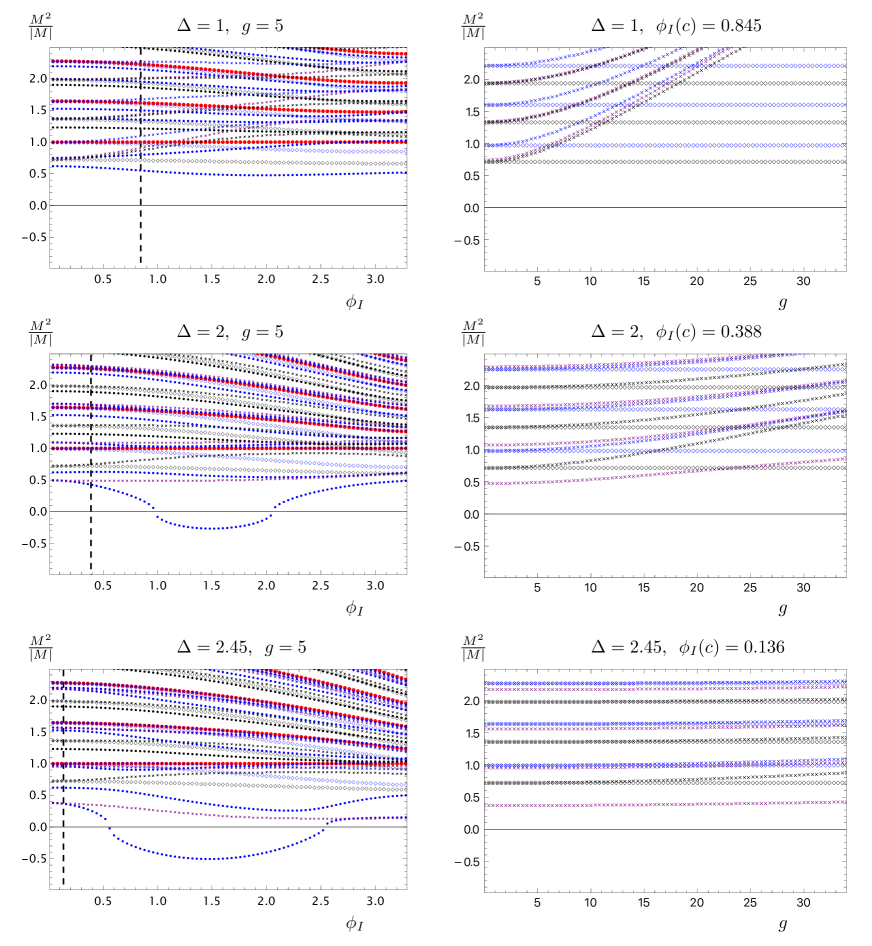
Figure 1: Mass spectrum $\frac{M^{2}}{|M|}$ of fluctuations, computed for confining backgrounds, with various choices of $\Delta$, as a function of the IR parameter $\phi_{I}$ for $g=5$ (left), and as a function of $g$ for $\phi_{I}=\phi_{I}(c)$ (right). For each $\Delta$, we show the spectrum of scalar (blue), pseudo-scalar (purple), vector (black), and tensor (red) states. The values of the IR and UV cutoffs in the calculations are respectively given by $\rho_{1}-\rho_{o}=10^{-9}$ and $\rho_{2}-\rho_{o}=5$, in all of the cases. The different symbols refer to the quantum numbers in respect to the unbroken $SO(4)$ symmetry: disks are used for singlets, and have already been reported in Ref. Elander:2022ebt , diamonds represent the $6$ of $SO(4)$, and crosses the $4$ of $SO(4)$. All masses are normalised to the mass of the lightest spin-2 state. Because the masses of the $SO(5)$ singlets do not depend on $g$, we do not repeat them in the right panels, which display only non-trivial $SO(5)$ multiplets.

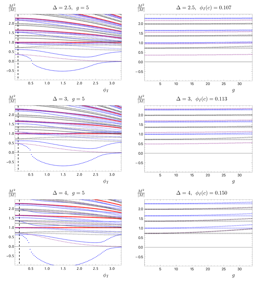
Figure 2: Mass spectrum $\frac{M^{2}}{|M|}$ of fluctuations, computed for confining backgrounds, with various choices of $\Delta$, as a function of the IR parameter $\phi_{I}$ for $g=5$ (left), and as a function of $g$ for $\phi_{I}=\phi_{I}(c)$ (right). For each $\Delta$, we show the spectrum of scalar (blue), pseudo-scalar (purple), vector (black), and tensor (red) states. The values of the IR and UV cutoffs in the calculations are respectively given by $\rho_{1}-\rho_{o}=10^{-9}$ and $\rho_{2}-\rho_{o}=5$, in all of the cases. The different symbols refer to the quantum numbers in respect to the unbroken $SO(4)$ symmetry: disks are used for singlets, and have already been reported in Ref. Elander:2022ebt , diamonds represent the $6$ of $SO(4)$, and crosses the $4$ of $SO(4)$. All masses are normalised to the mass of the lightest spin-2 state. Because the masses of the $SO(5)$ singlets do not depend on $g$, we do not repeat them in the right panels, which display only non-trivial $SO(5)$ multiplets.

In order to discuss our new results and provide an interpretation for them, we must first pause and explain the physical meaning of the parameters $\phi_{I}$ and $g$. The former is the parameter controlling the size of $SO(5)$ symmetry-breaking effects. Interestingly, despite the fact that $\phi$ obeys a second-order, non-linear differential equation, the requirement of regularity of the geometry at the end of the space imposes a non-trivial relation between the two free parameters that appear in a generic confining solution. For concreteness, we can think of them as the coefficients $\phi_{J}$ and $\phi_{V}$ appearing in the UV expansions, related to the explicit and spontaneous breaking of the symmetry on the field theory side. The numerical study in Ref. Elander:2022ebt demonstrates that for $0<\Delta<5$, there is a critical value of $\phi_{I}$, denoted $\phi_{I}(c)$, such that when $\phi_{I}>\phi_{I}(c)$ there exists an alternative classical solution that has a lower value of the free energy, for the same value of the source. This result demonstrates the existence of a phase transition. We choose to display $\phi_{I}=\phi_{I}(c)$ in the plots because this choice minimises the mass of the lightest spin-0 state.

The parameter $g$ controls the self-coupling of the bulk gauge fields. It is related to the coupling (and decay) of the composite vector mesons to two PNGBs, in the effective description of the dual field theory. But these statements require some more qualification, in view of the notational conventions we adopted. In the action, ${\cal S}_{6}$, we ignored a multiplicative factor of $2/\kappa^{2}$. In this paper, we are only solving classical background equations and linearised equations for the fluctuations around the chosen background solutions. In this process, $2/\kappa^{2}$ is just an overall factor that disappears from the final results. These classical results are exact if one takes the limit $\kappa\rightarrow 0$ while holding fixed $g$ and $\phi_{I}$. Close to the classical regime, perturbative corrections can be organised in loop diagrams, provided the coupling $g$ is not too strong. A naive estimate of the upper bound yields $\frac{3g^{2}\kappa^{2}}{256\pi^{3}}\ll 1$ Ponton:2012bi .

We show in Figs. 1 and 2 examples of mass spectra, for selected choices of $\Delta<5/2$ and $\Delta\geq 5/2$, respectively. Hence, for each representative choice of $\Delta$, we produce one plot in which we fix $g=5$ and vary $\phi_{I}$, and a second plot in which we fix $\phi_{I}=\phi_{I}(c)$, and vary $g$. We show all the states of the system, differentiating them by colour, and shape of the markers (for different $SO(4)$ representations). We also reproduce the results for the $SO(5)$ singlet, for completeness of the presentation, but also to set up their physics implication. More examples of the numerical results are presented in Appendix C.

For any values of $\Delta$, we find that the mass of the axial-vector states, transforming as $4$ of $SO(4)$, is larger than that of the vectors, and the difference grows with $g$. Also, the mass of the lightest PNGBs grows with $g$. When varying $\phi_{I}$ for $\Delta\lesssim 2$ and fixed $g$, the mass of the spin-0 states transforming as $4$ of $SO(4)$ grows with $\phi_{I}$. In field-theory terms, in this regime we are enhancing the effect of explicit symmetry breaking, compared to the spontaneous breaking, and there is no real sense in which these states are genuine PNGBs, despite having the right quantum numbers. But for $\Delta\geq 2.5$, we see that the mass of the lightest spin-0 states transforming as $4$ of $SO(4)$ can be made arbitrarily light, by choosing large values of $\phi_{I}$. Unfortunately though, the critical values of $\phi_{I}$ are rather small, and such large choices fall into the tachyonic part of the spectrum. The general conclusion of this exercise is that for all choices of $\Delta$ and $g$, if we restrict attention to the stable region of parameter space with $\phi_{I}\leq\phi_{I}(c)$, then the mass of the PNGBs shows no indications of being suppressed.

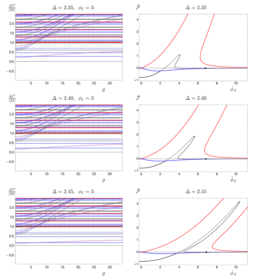
Figure 3: Mass spectrum $\frac{M^{2}}{|M|}$ of fluctuations, computed for confining backgrounds, for $\Delta=2.35$ (top), $\Delta=2.40$ (middle), and $\Delta=2.45$ (bottom), and $\phi_{I}=3$ as a function of $g$ (left), and free energy $\hat{\cal F}$ a function of the normalised source $\hat{\phi}_{J}$ (right). For the spectrum, scalar (blue), pseudo-scalar (purple), vector (black), and tensor (red) states are displayed as disks for $SO(4)$ singlets, as diamonds to represent the $6$ of $SO(4)$, and crosses for the $4$ of $SO(4)$. The values of the IR and UV cutoffs in the calculations are respectively given by $\rho_{1}-\rho_{o}=10^{-9}$ and $\rho_{2}-\rho_{o}=5$. All masses are normalised to the mass of the lightest spin-2 state. The definition of (normalised) free energy $\hat{\cal F}$ and (normalised) source $\hat{\phi}_{J}$ can be found in Ref. Elander:2022ebt . The black (stable), gray (metastable), and dashed black (tachyonic) regions of the curve refers to the confining solutions of interest, while red and blue curves refer to singular solutions. The black dots on the right panels denote the solutions with $\phi_{I}=3$.

Interestingly, we find something new when we focus attention on the case where $2\lesssim\Delta<2.5$. Ref. Elander:2022ebt found the existence of a metastable region of parameter space with large $\phi_{I}$, in which the lightest scalar is a dilaton. Here, we find that also the PNGBs, transforming as a $4$ of $SO(4)$, are light in this region of parameter space, their masses being suppressed in respect to the scale of all other bound states. This can be seen in the bottom-left panel of Fig. 1.

To demonstrate that the mass of these two states can be dialled to be arbitrarily small, compared to the typical mass scale of all other bound states, represented by the mass of the spin-2 particles, in Fig. 3, we display some more information about the choices $\Delta=2.35$, $\Delta=2.40$, and $\Delta=2.45$. We show in the left panels of the figure the dependence on $g$ of the spectrum, for a choice of $\phi_{I}=3$, large enough to fall in the portion of parameter space that contains a light dilaton together with a light set of PNGBs transforming as the $4$ of $SO(4)$.

While Ref. Elander:2022ebt , for such large values of $\phi_{I}$, found that the confining background solutions are metastable, we produce here three expanded and detailed plots showing that the free energy is almost degenerate with another branch of solutions. The plots on the right panels of Fig. 3 show the free energy $\hat{\cal F}$ computed using holographic renormalisation, as a function of the source $\hat{\phi}_{J}$, and normalised appropriately. The plots are expanded versions of those in Ref. Elander:2022ebt , and for these choices are obtained with the following relations:

$${\cal F} = -\frac{1}{40}e^{4A_{U}-\chi_{U}}\left(16\Delta\left(\frac{5}{2}-\Delta\right)\phi_{J}\phi_{V}-75\chi_{5}\right)\,,$$ (51)

$$\Lambda^{-1} \equiv \int_{\rho_{o}}^{\infty}\mbox{d}\rho\,e^{\chi(\rho)-A(\rho)}\,,$$ (52)

and the rescaling $\hat{\cal F}\equiv{\cal F}/\Lambda^{5}$, $\hat{\phi}_{J}\equiv\phi_{J}/\Lambda^{\Delta}$. We do not repeat here details, except for specifying that in the plots the choice $\phi_{I}=3$ is equivalent to confining solutions with $\hat{\phi}_{J}=6.78$ for $\Delta=2.35$, $\hat{\phi}_{J}=6.83$ for $\Delta=2.40$, and $\hat{\phi}_{J}=6.88$ for $\Delta=2.45$. The reason why we show these plots is that, besides the confining solutions, the analysis of the free energy carries over also for (singular) solutions respecting five-dimensional Poincaré invariance, and we can show a graphical comparison. In particular one can explicitly see that for $\phi_{I}=3$, in all three examples reported here, the confining solutions do not minimise the free energy. In the limit of large $\phi_{I}$, the metastable solutions might be long lived. Whether there are regions of parameter space that allow for the construction of a viable CHM, relying on the existence of a long-lived metastable vacuum, is an important question that would require a dedicated study.

While for small $\phi_{I}$ one could argue that the choice of potential adopted in this paper is as good as any, because it can be obtained as a power-expansion of more complicated potentials in the regime of small $\phi$, one expects model-dependence to affect the large $\phi_{I}$ region. Top-down models are not affected by this limitation. For example, Fig. 7 of Ref. Elander:2021kxk , shows the spectrum of a top-down model with $SO(5)$ symmetry breaking to $SO(4)$. The results at large $\phi_{I}$ qualitatively resembles, for large values of the VEV, the case $\Delta\geq 5/2$ of this paper, as for arbitrarily large values of $\phi_{I}$ the PNGBs become arbitrarily light, but also other states, including a tachyon, persist and their masses appear to be suppressed compared to the typical scale of the other bound state masses. We do not know if top-down models showing the feature we uncovered here exist, namely in which both dilaton and PNGBs are parametrically light, but there is no tachyon. Nevertheless, this is a new, unexpected result, which might have important phenomenological implications, that are worth studying in the future.

V Outlook

In this paper, we studied the spectrum of bound states carrying $SO(5)$ quantum numbers, in a strongly-coupled, confining field theory modelled by its higher-dimensional, weakly-coupled gravity dual. We paid particular attention to the states that have the correct quantum numbers to be identified as PNGBs, as the $SO(5)$ global symmetry of the field theory is broken both explicitly and spontaneously to its $SO(4)$ subgroup. We studied the spectrum as a function of three parameters. $\Delta$ is the parameter that, for $\Delta>5/2$, is interpreted in the field theory as the dimension of the scalar operator controlling $SO(5)$ breaking, and for $\Delta<5/2$ as the dimension of the coupling of the operator. $\phi_{I}$ is the parameter controlling the size of the symmetry breaking. And $g$ controls the self-coupling of vector fields, as well as their coupling to the PNGBs.

The main results of our analysis are two-fold. First, we showed that if we restrict our attention to the region of parameter space in which the confining solutions are stable, as identified in Ref. Elander:2022ebt , then neither the scalar $SO(5)$ singlet nor the $SO(4)$ multiplets are parametrically light, for any values of $\phi_{I}\leq\phi_{I}(c)$, $\Delta$, and $g$ that we considered. Second, we identified a metastable region of parameter space with $2\lesssim\Delta<2.5$ and large $\phi_{I}$, for which both the scalar $SO(5)$ singlet and the lightest spin-0 states transforming as $4$ of $SO(4)$ become arbitrarily light when approaching $\Delta\rightarrow 5/2$. In this case, the former is a dilaton, and the latter is a multiplet of PNGBs. The existence of this region of parameter space, and the fact that both types of particles are parametrically light, are both new and unexpected results, deserving further investigation.

This is the first step towards the construction of a composite Higgs model, in which the Higgs fields emerge as the PNGBs of a new strongly-coupled theory. The next step requires to couple the system to the SM gauge fields, and to study vacuum alignment in the theory, as a function of the strength of additional symmetry-breaking parameters, which in the gravity theory correspond to boundary-localised terms. Whether or not this will allow to explore other, enlarged regions of parameter space as viable for CHM model-building is not known, as is not known whether the presence of the dilaton in the metastable region of parameter space has phenomenologically relevant implications. These interesting questions will be addressed in future research.

Appendix A Basis of $SO(5)$ generators

For concreteness, we present here an example of a basis of $SO(5)$ generators, which we chose so that the first four generators $t^{\hat{A}}$, with $\hat{A}=1\,,\,\cdots\,,\,4$, span the the coset $SO(5)/SO(4)$, with the conventions in Eq. (19), while the unbroken $SO(4)$ is generated by $t^{\bar{A}}$, with $\bar{A}=5\,,\,\cdots\,,\,10$.

$$t^{1} = \frac{i}{2}\left(\begin{array}[]{ccccc}0&0&0&0&-1\\ 0&0&0&0&0\\ 0&0&0&0&0\\ 0&0&0&0&0\\ 1&0&0&0&0\end{array}\right)\,,\quad t^{2}=\frac{i}{2}\left(\begin{array}[]{ccccc}0&0&0&0&0\\ 0&0&0&0&-1\\ 0&0&0&0&0\\ 0&0&0&0&0\\ 0&1&0&0&0\end{array}\right)\,,\quad t^{3}=\frac{i}{2}\left(\begin{array}[]{ccccc}0&0&0&0&0\\ 0&0&0&0&0\\ 0&0&0&0&-1\\ 0&0&0&0&0\\ 0&0&1&0&0\end{array}\right)\,,\quad t^{4}=\frac{i}{2}\left(\begin{array}[]{ccccc}0&0&0&0&0\\ 0&0&0&0&0\\ 0&0&0&0&0\\ 0&0&0&0&-1\\ 0&0&0&1&0\end{array}\right)\,,$$ (73)

$$t^{5} = \frac{i}{2}\left(\begin{array}[]{ccccc}0&0&0&-1&0\\ 0&0&0&0&0\\ 0&0&0&0&0\\ 1&0&0&0&0\\ 0&0&0&0&0\end{array}\right)\,,\quad t^{6}=\frac{i}{2}\left(\begin{array}[]{ccccc}0&0&0&0&0\\ 0&0&0&-1&0\\ 0&0&0&0&0\\ 0&1&0&0&0\\ 0&0&0&0&0\end{array}\right)\,,\quad t^{7}=\frac{i}{2}\left(\begin{array}[]{ccccc}0&0&0&0&0\\ 0&0&0&0&0\\ 0&0&0&-1&0\\ 0&0&1&0&0\\ 0&0&0&0&0\end{array}\right)\,,$$ (89)

$$t^{8} = \frac{i}{2}\left(\begin{array}[]{ccccc}0&0&-1&0&0\\ 0&0&0&0&0\\ 1&0&0&0&0\\ 0&0&0&0&0\\ 0&0&0&0&0\end{array}\right)\,,\quad t^{9}=\frac{i}{2}\left(\begin{array}[]{ccccc}0&0&0&0&0\\ 0&0&-1&0&0\\ 0&1&0&0&0\\ 0&0&0&0&0\\ 0&0&0&0&0\end{array}\right)\,,\quad t^{10}=\frac{i}{2}\left(\begin{array}[]{ccccc}0&-1&0&0&0\\ 1&0&0&0&0\\ 0&0&0&0&0\\ 0&0&0&0&0\\ 0&0&0&0&0\end{array}\right)\,.\quad$$ (105)

Appendix B Asymptotic expansions of the fluctuations

The linearised equations governing the dynamics of the small fluctuations around the classical solutions are subject to boundary conditions that, as explained in the body of the paper, can be implemented by matching to the asymptotic expansion of the solutions, in a way that resembles the process of improvement in lattice field theory. It is hence useful to report here such asymptotic expansions. We find it convenient to include also the $SO(5)$ singlets, together with the $SO(4)$ multiplets.

B.1 IR expansions

We start from the IR expansion of the fluctuations. For convenience, we put $\rho_{o}=0$ and $A_{I}=0$ in this subsection, while setting $\chi_{I}=0$ in order to avoid a conical singularity. We then expand the solutions of the linearised equations in powers of small $\rho$. We can write the expansion for a general value of $\Delta$.

For the scalar fluctuations, we find

$$\mathfrak{a}^{1}= \ \mathfrak{a}^{1}_{I,0}+\mathfrak{a}^{1}_{I,l}\log(\rho)+\frac{1}{4}\rho^{2}\bigg{[}-\frac{1}{4}\Delta\left(\mathfrak{a}^{1}_{I,0}\left(\Delta\left(15\phi_{I}^{2}-4\right)+20\right)+6\phi_{I}(\mathfrak{a}^{2}_{I,0}-\mathfrak{a}^{2}_{I,l})\left(\Delta\left(5\phi_{I}^{2}-4\right)+20\right)\right)$$

$$+q^{2}(\mathfrak{a}^{1}_{I,0}-\mathfrak{a}^{1}_{I,l})-\frac{1}{48}\mathfrak{a}^{1}_{I,l}\left(\Delta\left(25\Delta\phi_{I}^{4}+20(10-11\Delta)\phi_{I}^{2}+48(\Delta-5)\right)+400\right)$$

$$+\log(\rho)\left(\mathfrak{a}^{1}_{I,l}\left(-\frac{15\Delta^{2}\phi_{I}^{2}}{4}+(\Delta-5)\Delta+q^{2}\right)-\frac{3}{2}\mathfrak{a}^{2}_{I,l}\Delta\phi_{I}\left(\Delta\left(5\phi_{I}^{2}-4\right)+20\right)\right)\bigg{]}+\mathcal{O}\left(\rho^{4}\right)\,,$$ (106)

$$\mathfrak{a}^{2}= \ \mathfrak{a}^{2}_{I,0}+\mathfrak{a}^{2}_{I,l}\log(\rho)+\frac{1}{4}\rho^{2}\bigg{[}-\frac{1}{4}\Delta\phi_{I}(\mathfrak{a}^{1}_{I,0}-\mathfrak{a}^{1}_{I,l})\left(\Delta\left(5\phi_{I}^{2}-4\right)+20\right)+q^{2}(\mathfrak{a}^{2}_{I,0}-\mathfrak{a}^{2}_{I,l})$$

$$-\frac{3}{8}\mathfrak{a}^{2}_{I,0}\left(\Delta\phi_{I}^{2}\left(\Delta\left(5\phi_{I}^{2}-8\right)+40\right)+80\right)+\frac{13}{48}\mathfrak{a}^{2}_{I,l}\left(\Delta\phi_{I}^{2}\left(\Delta\left(5\phi_{I}^{2}-8\right)+40\right)+80\right)$$

$$+\log(\rho)\left(-\frac{5}{4}\mathfrak{a}^{1}_{I,l}\Delta^{2}\phi_{I}^{3}+\mathfrak{a}^{1}_{I,l}(\Delta-5)\Delta\phi_{I}+\mathfrak{a}^{2}_{I,l}\left(-\frac{15}{8}\Delta^{2}\phi_{I}^{4}+3(\Delta-5)\Delta\phi_{I}^{2}+q^{2}-30\right)\right)\bigg{]}+\mathcal{O}\left(\rho^{4}\right)\,,$$ (107)

$$\mathfrak{a}^{3}= \ \mathfrak{a}^{3}_{I,0}+\rho^{2}\left(\frac{1}{2}\mathfrak{a}^{3}_{I,0}q^{2}\log(\rho)+\mathfrak{a}^{3}_{I,2}\right)+\mathcal{O}\left(\rho^{4}\right)\,,$$ (108)

$$\mathfrak{a}^{4}= \ \mathfrak{a}^{4}_{I,0}+\rho^{2}\left(\frac{1}{2}\mathfrak{a}^{4}_{I,0}\left(q^{2}+\frac{g^{2}\phi_{I}^{2}}{4}\right)\log(\rho)+\mathfrak{a}^{4}_{I,2}\right)+\mathcal{O}\left(\rho^{4}\right)\,.$$ (109)

For the pseudo-scalar fluctuations, we find

$$\mathfrak{p}=\mathfrak{p}_{I,0}+\rho^{2}\left[\mathfrak{p}_{I,2}+\frac{1}{2}\mathfrak{p}_{I,0}\left(q^{2}+\frac{g^{2}}{4}\phi_{I}^{2}\right)\log(\rho)\right]+\mathcal{O}\left(\rho^{4}\right)\,.$$ (110)

For the vector fluctuations, we find

$$\mathfrak{v}^{1}= \ \mathfrak{v}^{1}_{I,-2}\rho^{-2}+\frac{1}{2}q^{2}\mathfrak{v}^{1}_{I,-2}\log(\rho)+\mathfrak{v}^{1}_{I,0}+\frac{1}{12288}\rho^{2}\Big{[}1536q^{2}\mathfrak{v}^{1}_{I,0}+80\Delta^{2}\mathfrak{v}^{1}_{I,-2}\phi_{I}^{4}\left(2\left(8\Delta^{2}-50\Delta+75\right)-3q^{2}\right)$$

$$+128(\Delta-5)\Delta\mathfrak{v}^{1}_{I,-2}\phi_{I}^{2}\left(-3(\Delta-5)\Delta+3q^{2}-50\right)-64\left(9q^{4}+60q^{2}-500\right)\mathfrak{v}^{1}_{I,-2}+125\Delta^{4}\mathfrak{v}^{1}_{I,-2}\phi_{I}^{8}$$

$$-1000(\Delta-2)\Delta^{3}\mathfrak{v}^{1}_{I,-2}\phi_{I}^{6}+768q^{4}\mathfrak{v}^{1}_{I,-2}\log(\rho)\Big{]}+\mathcal{O}\left(\rho^{4}\right)\,,$$ (111)

$$\mathfrak{v}^{2}= \ \mathfrak{v}^{2}_{I,0}+\mathfrak{v}^{2}_{I,l}\log(\rho)+\frac{1}{96}\rho^{2}\Big{[}24q^{2}(\mathfrak{v}^{2}_{I,0}-\mathfrak{v}^{2}_{I,l})+\mathfrak{v}^{2}_{I,l}\left(-5\Delta^{2}\phi_{I}^{4}+8(\Delta-5)\Delta\phi_{I}^{2}-80\right)$$

$$+24q^{2}\mathfrak{v}^{2}_{I,l}\log(\rho)\Big{]}+\mathcal{O}\left(\rho^{4}\right)\,,$$ (112)

$$\mathfrak{v}^{3}= \ \mathfrak{v}^{3}_{I,0}+\mathfrak{v}^{3}_{I,l}\log(\rho)+\frac{1}{96}\rho^{2}\Big{[}\left(24q^{2}+6g^{2}\phi_{I}^{2}\right)\mathfrak{v}^{3}_{I,0}+\left(-80-24q^{2}-6g^{2}\phi_{I}^{2}-40\Delta\phi_{I}^{2}+\Delta^{2}\left(8\phi_{I}^{2}-5\phi_{I}^{4}\right)\right)\mathfrak{v}^{3}_{I,l}$$

$$+\left(24q^{2}+6g^{2}\phi_{I}^{2}\right)\log(\rho)\mathfrak{v}^{3}_{I,l}\Big{]}+\mathcal{O}\left(\rho^{4}\right)\,.$$ (113)

For the tensor fluctuations, we find

$$\mathfrak{e}=\mathfrak{e}_{I,0}+\mathfrak{e}_{I,l}\log(\rho)+\frac{1}{192}\rho^{2}\Big{[}48q^{2}(\mathfrak{e}_{I,0}-\mathfrak{e}_{I,l})-25\Delta^{2}\mathfrak{e}_{I,l}\phi_{I}^{4}+40(\Delta-5)\Delta\mathfrak{e}_{I,l}\phi_{I}^{2}-400\mathfrak{e}_{I,l}+48\mathfrak{e}_{I,l}q^{2}\log(\rho)\Big{]}+\mathcal{O}\left(\rho^{4}\right)\,.$$ (114)

B.2 UV expansions

The expansions for large $\rho$, in the UV regime of the dual field-theory interpretation, depend non-trivially on the parameter $\Delta$. For illustration purposes, in this subsection we set $\Delta=3$, and $A_{U}=0=\chi_{U}$. We write the expansions in terms of $z\equiv e^{-\rho}$.

For the scalar fluctuations, we find

$$\mathfrak{a}^{1}= \ \mathfrak{a}^{1}_{2}z^{2}+\mathfrak{a}^{1}_{3}z^{3}+\frac{1}{2}\mathfrak{a}^{1}_{2}q^{2}z^{4}+\frac{1}{6}\mathfrak{a}^{1}_{3}q^{2}z^{5}+\frac{1}{48}\mathfrak{a}^{1}_{2}\left(2q^{4}-99\phi_{J}^{2}\right)z^{6}+\mathcal{O}\left(z^{7}\right)\,,$$ (115)

$$\mathfrak{a}^{2}= \ \mathfrak{a}^{2}_{0}-\frac{1}{6}\mathfrak{a}^{2}_{0}q^{2}z^{2}+\frac{1}{24}\mathfrak{a}^{2}_{0}q^{4}z^{4}+\mathfrak{a}^{2}_{5}z^{5}+\frac{1}{144}\mathfrak{a}^{2}_{0}q^{2}\left(q^{4}-14\phi_{J}^{2}\right)z^{6}+\mathcal{O}\left(z^{7}\right)\,,$$ (116)

$$\mathfrak{a}^{3}= \ \mathfrak{a}^{3}_{0}-\frac{1}{2}\mathfrak{a}^{3}_{0}q^{2}z^{2}+\mathfrak{a}^{3}_{3}z^{3}-\frac{1}{8}\mathfrak{a}^{3}_{0}q^{4}z^{4}+\frac{1}{10}\mathfrak{a}^{3}_{3}q^{2}z^{5}-\frac{1}{144}\mathfrak{a}^{3}_{0}q^{2}\left(q^{4}+10\phi_{J}^{2}\right)z^{6}+\mathcal{O}\left(z^{7}\right)\,,$$ (117)

$$\mathfrak{a}^{4}= \ \mathfrak{a}^{4}_{0}-\frac{1}{2}\mathfrak{a}^{4}_{0}q^{2}z^{2}+\mathfrak{a}^{4}_{3}z^{3}+\frac{1}{16}\mathfrak{a}^{4}_{0}\left(g^{2}\phi_{J}^{2}-2q^{4}\right)z^{4}+\frac{1}{20}\left(\mathfrak{a}^{4}_{0}g^{2}\phi_{J}\phi_{V}+2\mathfrak{a}^{4}_{3}q^{2}\right)z^{5}$$

$$-\frac{1}{288}\mathfrak{a}^{4}_{0}\left(2q^{6}+(20+g^{2})q^{2}\phi_{J}^{2}-4g^{2}\phi_{V}^{2}\right)z^{6}+\mathcal{O}\left(z^{7}\right)\,.$$ (118)

For the pseudo-scalar fluctuations, we find

$$\mathfrak{p}= \ \mathfrak{p}_{0}+\mathfrak{p}_{1}z+\left(\frac{\mathfrak{p}_{0}q^{2}}{2}+\frac{\mathfrak{p}_{1}\phi_{V}}{\phi_{J}}\right)z^{2}+\frac{2\mathfrak{p}_{0}q^{2}\phi_{J}\phi_{V}+\mathfrak{p}_{1}q^{2}\phi_{J}^{2}+2\mathfrak{p}_{1}\phi_{V}^{2}}{6\phi_{J}^{2}}z^{3}$$

$$+\frac{\mathfrak{p}_{0}\left(q^{4}\phi_{J}+\frac{g^{2}\phi_{J}^{3}}{2}\right)+4\mathfrak{p}_{1}q^{2}\phi_{V}}{24\phi_{J}}z^{4}+\mathcal{O}\left(z^{5}\right)\,.$$ (119)

For the vector fluctuations, we find

$$\mathfrak{v}^{1}= \ \mathfrak{v}^{1}_{0}-\frac{1}{6}q^{2}\mathfrak{v}^{1}_{0}z^{2}+\frac{1}{24}q^{4}\mathfrak{v}^{1}_{0}z^{4}+\mathfrak{v}^{1}_{5}z^{5}+\frac{1}{144}q^{2}\mathfrak{v}^{1}_{0}\left(q^{4}-14\phi_{J}^{2}\right)z^{6}$$

$$+\frac{1}{70}q^{2}(70\mathfrak{v}^{1}_{0}\chi_{5}-2\mathfrak{v}^{1}_{0}\phi_{J}\phi_{V}+5\mathfrak{v}^{1}_{5})z^{7}+\mathcal{O}\left(z^{8}\right)\,,$$ (120)

$$\mathfrak{v}^{2}= \ \mathfrak{v}^{2}_{0}-\frac{1}{2}q^{2}\mathfrak{v}^{2}_{0}z^{2}+\mathfrak{v}^{2}_{3}z^{3}-\frac{1}{8}q^{4}\mathfrak{v}^{2}_{0}z^{4}+\frac{1}{10}q^{2}\mathfrak{v}^{2}_{3}z^{5}-\frac{1}{144}q^{2}\mathfrak{v}^{2}_{0}\left(q^{4}+10\phi_{J}^{2}\right)z^{6}$$

$$+\frac{1}{1400}\left(5(q^{4}+45\phi_{J}^{2})\mathfrak{v}^{2}_{3}+6q^{2}\mathfrak{v}^{2}_{0}(75\chi_{5}-26\phi_{J}\phi_{V})\right)z^{7}+\mathcal{O}\left(z^{8}\right)\,,$$ (121)

$$\mathfrak{v}^{3}= \ \mathfrak{v}^{3}_{0}-\frac{1}{2}q^{2}\mathfrak{v}^{3}_{0}z^{2}+\mathfrak{v}^{3}_{3}z^{3}-\frac{1}{8}\mathfrak{v}^{3}_{0}\left(q^{4}-\frac{g^{2}}{2}\phi_{J}^{2}\right)z^{4}+\frac{1}{10}\left(q^{2}\mathfrak{v}^{3}_{3}+\frac{g^{2}}{2}\mathfrak{v}^{3}_{0}\phi_{J}\phi_{V}\right)z^{5}+\mathcal{O}\left(z^{6}\right)\,.$$ (122)

For the tensor fluctuations, we find

$$\mathfrak{e}=\mathfrak{e}_{0}-\frac{1}{6}\mathfrak{e}_{0}q^{2}z^{2}+\frac{1}{24}\mathfrak{e}_{0}q^{4}z^{4}+\mathfrak{e}_{5}z^{5}+\mathcal{O}\left(z^{6}\right)\,.$$ (123)

The choice $\Delta=3$ yields a particularly simple expansion in powers of $z$. In the process of carrying out the numerical calculations for this paper, we computed the UV expansions for all values of $\Delta$ for which we plot the spectrum. We do not report all of these expansions here, but we notice that for special choices of $\Delta$ the formal expansion changes, to include also logarithmic terms in the form $z^{n}\log^{m}(z)$.

Appendix C More mass spectra

In this Appendix, we report a few additional examples of spectra, in Figs. 4–6. The choices of $\Delta$ are such as to include the entirety of the catalogue in Ref. Elander:2022ebt . We fix the indicative value $g=5$ in all plots. Qualitatively, all these plots resemble at least one of those in the main body, though quantitative features may be amplified or suppressed by changes in $\Delta$.

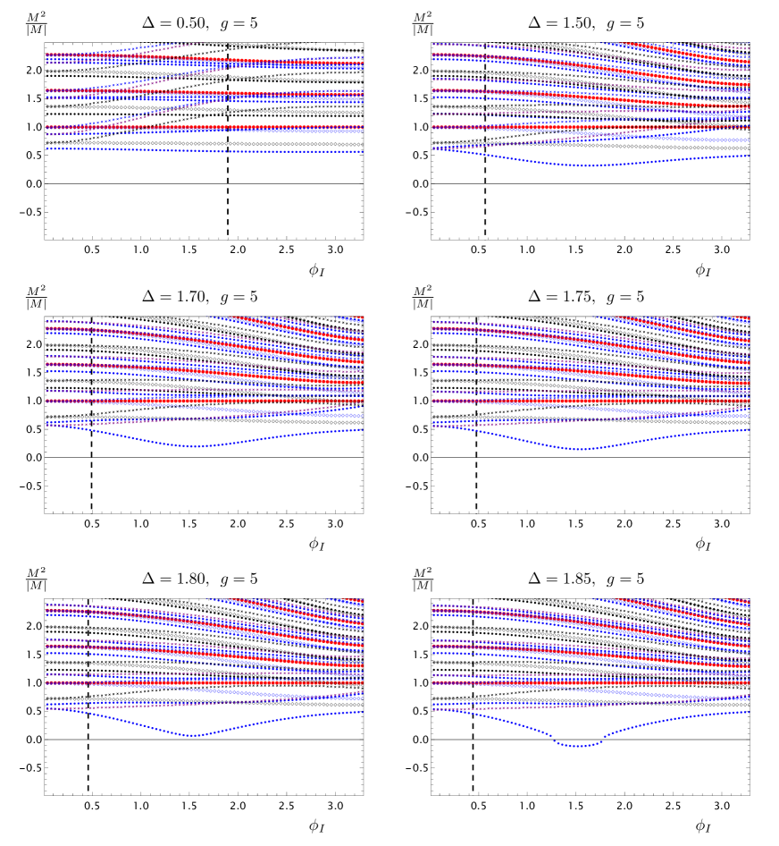
Figure 4: Mass spectrum $\frac{M^{2}}{|M|}$ of fluctuations, computed for confining backgrounds, with various choices of $\Delta$, as a function of the IR parameter $\phi_{I}$ for $g=5$. For each $\Delta$, we show the spectrum of scalar (blue), pseudo-scalar (purple), vector (black), and tensor (red) states. The values of the IR and UV cutoffs in the calculations are respectively given by $\rho_{1}-\rho_{o}=10^{-9}$ and $\rho_{2}-\rho_{o}=5$, in all of the cases. The different symbols refer to the quantum numbers in respect to the unbroken $SO(4)$ symmetry: disks are used for singlets, and have already been reported in Ref. Elander:2022ebt , diamonds represent the $6$ of $SO(4)$, and crosses the $4$ of $SO(4)$. All masses are normalised to the mass of the lightest spin-2 state.

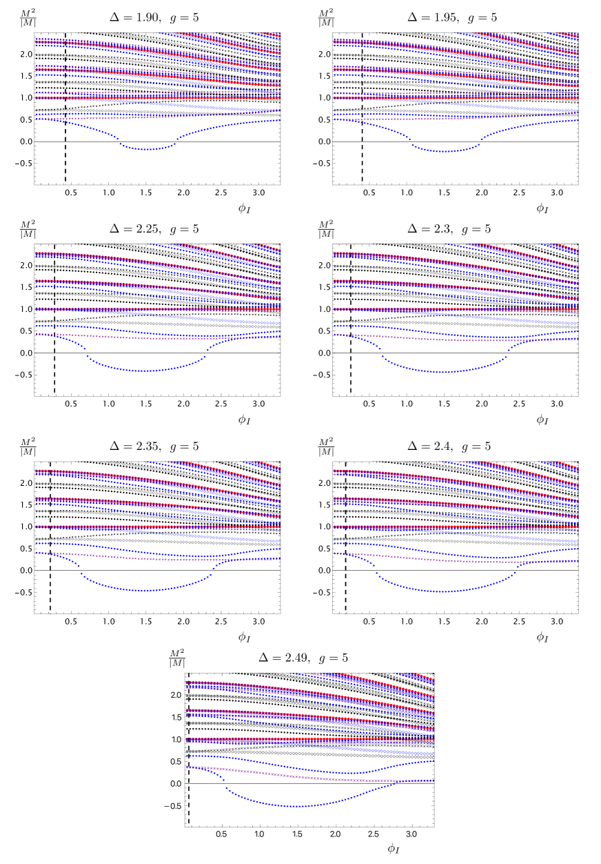
Figure 5: Mass spectrum $\frac{M^{2}}{|M|}$ of fluctuations, computed for confining backgrounds, with various choices of $\Delta$, as a function of the IR parameter $\phi_{I}$ for $g=5$. For each $\Delta$, we show the spectrum of scalar (blue), pseudo-scalar (purple), vector (black), and tensor (red) states. The values of the IR and UV cutoffs in the calculations are respectively given by $\rho_{1}-\rho_{o}=10^{-9}$ and $\rho_{2}-\rho_{o}=5$, in all of the cases. The different symbols refer to the quantum numbers in respect to the unbroken $SO(4)$ symmetry: disks are used for singlets, and have already been reported in Ref. Elander:2022ebt , diamonds represent the $6$ of $SO(4)$, and crosses the $4$ of $SO(4)$. All masses are normalised to the mass of the lightest spin-2 state.

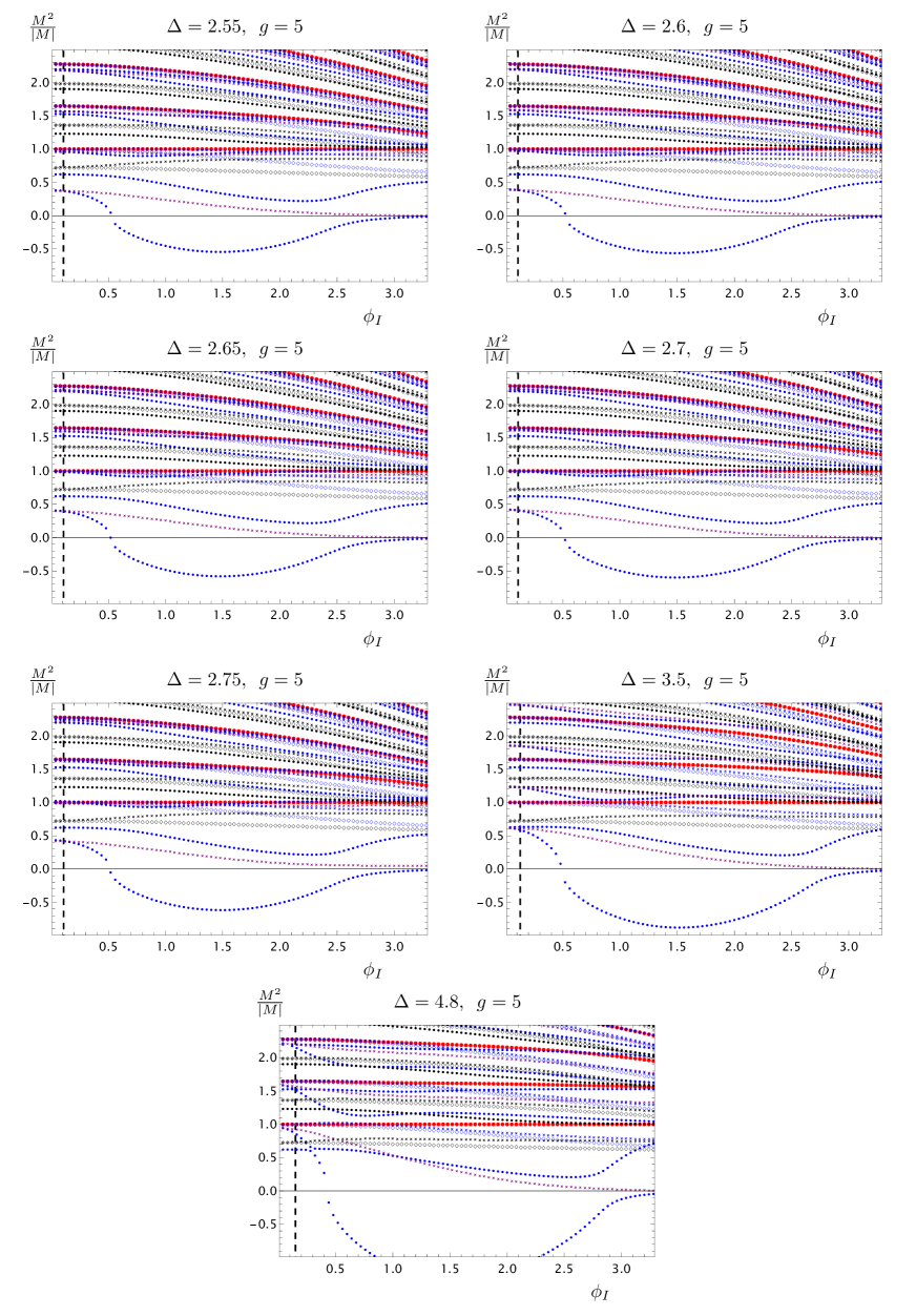
Figure 6: Mass spectrum $\frac{M^{2}}{|M|}$ of fluctuations, computed for confining backgrounds, with various choices of $\Delta$, as a function of the IR parameter $\phi_{I}$ for $g=5$. For each $\Delta$, we show the spectrum of scalar (blue), pseudo-scalar (purple), vector (black), and tensor (red) states. The values of the IR and UV cutoffs in the calculations are respectively given by $\rho_{1}-\rho_{o}=10^{-9}$ and $\rho_{2}-\rho_{o}=5$, in all of the cases. The different symbols refer to the quantum numbers in respect to the unbroken $SO(4)$ symmetry: disks are used for singlets, and have already been reported in Ref. Elander:2022ebt , diamonds represent the $6$ of $SO(4)$, and crosses the $4$ of $SO(4)$. All masses are normalised to the mass of the lightest spin-2 state.

References

- (1) G. Aad et al. [ATLAS Collaboration], “Observation of a new particle in the search for the Standard Model Higgs boson with the ATLAS detector at the LHC,” Phys. Lett. B 716, 1 (2012) doi:10.1016/j.physletb.2012.08.020 [arXiv:1207.7214 [hep-ex]].
- (2) S. Chatrchyan et al. [CMS Collaboration], “Observation of a new boson at a mass of 125 GeV with the CMS experiment at the LHC,” Phys. Lett. B 716, 30 (2012) doi:10.1016/j.physletb.2012.08.021 [arXiv:1207.7235 [hep-ex]].
- (3) D. B. Kaplan and H. Georgi, “ Breaking by Vacuum Misalignment,” Phys. Lett. 136B, 183 (1984). doi:10.1016/0370-2693(84)91177-8
- (4) H. Georgi and D. B. Kaplan, “Composite Higgs and Custodial SU(2),” Phys. Lett. 145B, 216 (1984). doi:10.1016/0370-2693(84)90341-1
- (5) M. J. Dugan, H. Georgi and D. B. Kaplan, “Anatomy of a Composite Higgs Model,” Nucl. Phys. B 254, 299 (1985). doi:10.1016/0550-3213(85)90221-4
- (6) G. Panico and A. Wulzer, “The Composite Nambu-Goldstone Higgs,” Lect. Notes Phys. 913, pp.1 (2016) doi:10.1007/978-3-319-22617-0 [arXiv:1506.01961 [hep-ph]].
- (7) O. Witzel, “Review on Composite Higgs Models,” PoS LATTICE 2018, 006 (2019) doi:10.22323/1.334.0006 [arXiv:1901.08216 [hep-lat]].
- (8) G. Cacciapaglia, C. Pica and F. Sannino, “Fundamental Composite Dynamics: A Review,” Phys. Rept. 877, 1-70 (2020) doi:10.1016/j.physrep.2020.07.002 [arXiv:2002.04914 [hep-ph]].
- (9) G. Ferretti and D. Karateev, “Fermionic UV completions of Composite Higgs models,” JHEP 03, 077 (2014) doi:10.1007/JHEP03(2014)077 [arXiv:1312.5330 [hep-ph]].
- (10) G. Ferretti, “Gauge theories of Partial Compositeness: Scenarios for Run-II of the LHC,” JHEP 06, 107 (2016) doi:10.1007/JHEP06(2016)107 [arXiv:1604.06467 [hep-ph]].
- (11) G. Cacciapaglia, G. Ferretti, T. Flacke and H. Serôdio, “Light scalars in composite Higgs models,” Front. Phys. 7, 22 (2019) doi:10.3389/fphy.2019.00022 [arXiv:1902.06890 [hep-ph]].
- (12) E. Katz, A. E. Nelson and D. G. E. Walker, “The Intermediate Higgs,” JHEP 0508, 074 (2005) doi:10.1088/1126-6708/2005/08/074 [hep-ph/0504252].
- (13) R. Barbieri, B. Bellazzini, V. S. Rychkov and A. Varagnolo, “The Higgs boson from an extended symmetry,” Phys. Rev. D 76, 115008 (2007) doi:10.1103/PhysRevD.76.115008 [arXiv:0706.0432 [hep-ph]].
- (14) P. Lodone, “Vector-like quarks in a composite Higgs model,” JHEP 0812, 029 (2008) doi:10.1088/1126-6708/2008/12/029 [arXiv:0806.1472 [hep-ph]].
- (15) B. Gripaios, A. Pomarol, F. Riva and J. Serra, “Beyond the Minimal Composite Higgs Model,” JHEP 0904, 070 (2009) doi:10.1088/1126-6708/2009/04/070 [arXiv:0902.1483 [hep-ph]].
- (16) J. Mrazek, A. Pomarol, R. Rattazzi, M. Redi, J. Serra and A. Wulzer, “The Other Natural Two Higgs Doublet Model,” Nucl. Phys. B 853, 1-48 (2011) doi:10.1016/j.nuclphysb.2011.07.008 [arXiv:1105.5403 [hep-ph]].
- (17) D. Marzocca, M. Serone and J. Shu, “General Composite Higgs Models,” JHEP 1208, 013 (2012) doi:10.1007/JHEP08(2012)013 [arXiv:1205.0770 [hep-ph]].
- (18) C. Grojean, O. Matsedonskyi and G. Panico, “Light top partners and precision physics,” JHEP 1310, 160 (2013) doi:10.1007/JHEP10(2013)160 [arXiv:1306.4655 [hep-ph]].
- (19) J. Barnard, T. Gherghetta and T. S. Ray, “UV descriptions of composite Higgs models without elementary scalars,” JHEP 1402, 002 (2014) doi:10.1007/JHEP02(2014)002 [arXiv:1311.6562 [hep-ph]].
- (20) G. Cacciapaglia and F. Sannino, “Fundamental Composite (Goldstone) Higgs Dynamics,” JHEP 1404, 111 (2014) doi:10.1007/JHEP04(2014)111 [arXiv:1402.0233 [hep-ph]].
- (21) G. Ferretti, “UV Completions of Partial Compositeness: The Case for a SU(4) Gauge Group,” JHEP 06, 142 (2014) doi:10.1007/JHEP06(2014)142 [arXiv:1404.7137 [hep-ph]].
- (22) A. Arbey, G. Cacciapaglia, H. Cai, A. Deandrea, S. Le Corre and F. Sannino, “Fundamental Composite Electroweak Dynamics: Status at the LHC,” Phys. Rev. D 95, no. 1, 015028 (2017) doi:10.1103/PhysRevD.95.015028 [arXiv:1502.04718 [hep-ph]].
- (23) G. von Gersdorff, E. Pontón and R. Rosenfeld, “The Dynamical Composite Higgs,” JHEP 06 (2015), 119 doi:10.1007/JHEP06(2015)119 [arXiv:1502.07340 [hep-ph]].
- (24) L. Vecchi, “A dangerous irrelevant UV-completion of the composite Higgs,” JHEP 02, 094 (2017) doi:10.1007/JHEP02(2017)094 [arXiv:1506.00623 [hep-ph]].
- (25) G. Cacciapaglia, H. Cai, A. Deandrea, T. Flacke, S. J. Lee and A. Parolini, “Composite scalars at the LHC: the Higgs, the Sextet and the Octet,” JHEP 1511, 201 (2015) doi:10.1007/JHEP11(2015)201 [arXiv:1507.02283 [hep-ph]].
- (26) T. Ma and G. Cacciapaglia, “Fundamental Composite 2HDM: SU(N) with 4 flavours,” JHEP 03, 211 (2016) doi:10.1007/JHEP03(2016)211 [arXiv:1508.07014 [hep-ph]].
- (27) F. Feruglio, B. Gavela, K. Kanshin, P. A. N. Machado, S. Rigolin and S. Saa, “The minimal linear sigma model for the Goldstone Higgs,” JHEP 1606, 038 (2016) doi:10.1007/JHEP06(2016)038 [arXiv:1603.05668 [hep-ph]].
- (28) T. DeGrand, M. Golterman, E. T. Neil and Y. Shamir, “One-loop Chiral Perturbation Theory with two fermion representations,” Phys. Rev. D 94, no. 2, 025020 (2016) doi:10.1103/PhysRevD.94.025020 [arXiv:1605.07738 [hep-ph]].
- (29) S. Fichet, G. von Gersdorff, E. Pontòn and R. Rosenfeld, “The Excitation of the Global Symmetry-Breaking Vacuum in Composite Higgs Models,” JHEP 1609, 158 (2016) doi:10.1007/JHEP09(2016)158 [arXiv:1607.03125 [hep-ph]].
- (30) J. Galloway, A. L. Kagan and A. Martin, “A UV complete partially composite-pNGB Higgs,” Phys. Rev. D 95, no. 3, 035038 (2017) doi:10.1103/PhysRevD.95.035038 [arXiv:1609.05883 [hep-ph]].
- (31) A. Agugliaro, O. Antipin, D. Becciolini, S. De Curtis and M. Redi, “UV complete composite Higgs models,” Phys. Rev. D 95, no. 3, 035019 (2017) doi:10.1103/PhysRevD.95.035019 [arXiv:1609.07122 [hep-ph]].
- (32) A. Belyaev, G. Cacciapaglia, H. Cai, G. Ferretti, T. Flacke, A. Parolini and H. Serodio, “Di-boson signatures as Standard Candles for Partial Compositeness,” JHEP 01, 094 (2017) doi:10.1007/JHEP01(2017)094 [arXiv:1610.06591 [hep-ph]].
- (33) N. Bizot, M. Frigerio, M. Knecht and J. L. Kneur, “Nonperturbative analysis of the spectrum of meson resonances in an ultraviolet-complete composite-Higgs model,” Phys. Rev. D 95, no. 7, 075006 (2017) doi:10.1103/PhysRevD.95.075006 [arXiv:1610.09293 [hep-ph]].
- (34) C. Csaki, T. Ma and J. Shu, “Maximally Symmetric Composite Higgs Models,” Phys. Rev. Lett. 119, no. 13, 131803 (2017) doi:10.1103/PhysRevLett.119.131803 [arXiv:1702.00405 [hep-ph]].
- (35) M. Chala, G. Durieux, C. Grojean, L. de Lima and O. Matsedonskyi, “Minimally extended SILH,” JHEP 1706, 088 (2017) doi:10.1007/JHEP06(2017)088 [arXiv:1703.10624 [hep-ph]].
- (36) M. Golterman and Y. Shamir, “Effective potential in ultraviolet completions for composite Higgs models,” Phys. Rev. D 97, no. 9, 095005 (2018) doi:10.1103/PhysRevD.97.095005 [arXiv:1707.06033 [hep-ph]].
- (37) C. Csaki, T. Ma and J. Shu, “Trigonometric Parity for Composite Higgs Models,” Phys. Rev. Lett. 121, no. 23, 231801 (2018) doi:10.1103/PhysRevLett.121.231801 [arXiv:1709.08636 [hep-ph]].
- (38) T. Alanne, D. Buarque Franzosi and M. T. Frandsen, “A partially composite Goldstone Higgs,” Phys. Rev. D 96, no. 9, 095012 (2017) doi:10.1103/PhysRevD.96.095012 [arXiv:1709.10473 [hep-ph]].
- (39) T. Alanne, D. Buarque Franzosi, M. T. Frandsen, M. L. A. Kristensen, A. Meroni and M. Rosenlyst, “Partially composite Higgs models: Phenomenology and RG analysis,” JHEP 1801, 051 (2018) doi:10.1007/JHEP01(2018)051 [arXiv:1711.10410 [hep-ph]].
- (40) F. Sannino, P. Stangl, D. M. Straub and A. E. Thomsen, “Flavor Physics and Flavor Anomalies in Minimal Fundamental Partial Compositeness,” Phys. Rev. D 97, no. 11, 115046 (2018) doi:10.1103/PhysRevD.97.115046 [arXiv:1712.07646 [hep-ph]].
- (41) T. Alanne, N. Bizot, G. Cacciapaglia and F. Sannino, “Classification of NLO operators for composite Higgs models,” Phys. Rev. D 97, no. 7, 075028 (2018) doi:10.1103/PhysRevD.97.075028 [arXiv:1801.05444 [hep-ph]].
- (42) N. Bizot, G. Cacciapaglia and T. Flacke, “Common exotic decays of top partners,” JHEP 1806, 065 (2018) doi:10.1007/JHEP06(2018)065 [arXiv:1803.00021 [hep-ph]].
- (43) C. Cai, G. Cacciapaglia and H. H. Zhang, “Vacuum alignment in a composite 2HDM,” JHEP 1901, 130 (2019) doi:10.1007/JHEP01(2019)130 [arXiv:1805.07619 [hep-ph]].
- (44) A. Agugliaro, G. Cacciapaglia, A. Deandrea and S. De Curtis, “Vacuum misalignment and pattern of scalar masses in the SU(5)/SO(5) composite Higgs model,” JHEP 1902, 089 (2019) doi:10.1007/JHEP02(2019)089 [arXiv:1808.10175 [hep-ph]].
- (45) D. Buarque Franzosi, G. Cacciapaglia and A. Deandrea, “Sigma-assisted low scale composite Goldstone–Higgs,” Eur. Phys. J. C 80, no.1, 28 (2020) doi:10.1140/epjc/s10052-019-7572-z [arXiv:1809.09146 [hep-ph]].
- (46) G. Cacciapaglia, T. Ma, S. Vatani and Y. Wu, “Towards a fundamental safe theory of composite Higgs and Dark Matter,” Eur. Phys. J. C 80, no.11, 1088 (2020) doi:10.1140/epjc/s10052-020-08648-7 [arXiv:1812.04005 [hep-ph]].
- (47) H. Gertov, A. E. Nelson, A. Perko and D. G. E. Walker, “Lattice-Friendly Gauge Completion of a Composite Higgs with Top Partners,” JHEP 1902, 181 (2019) doi:10.1007/JHEP02(2019)181 [arXiv:1901.10456 [hep-ph]].
- (48) V. Ayyar, M. F. Golterman, D. C. Hackett, W. Jay, E. T. Neil, Y. Shamir and B. Svetitsky, “Radiative Contribution to the Composite-Higgs Potential in a Two-Representation Lattice Model,” Phys. Rev. D 99, no. 9, 094504 (2019) doi:10.1103/PhysRevD.99.094504 [arXiv:1903.02535 [hep-lat]].
- (49) G. Cacciapaglia, H. Cai, A. Deandrea and A. Kushwaha, “Composite Higgs and Dark Matter Model in SU(6)/SO(6),” JHEP 1910, 035 (2019) doi:10.1007/JHEP10(2019)035 [arXiv:1904.09301 [hep-ph]].
- (50) D. Buarque Franzosi and G. Ferretti, “Anomalous dimensions of potential top-partners,” SciPost Phys. 7, no. 3, 027 (2019) doi:10.21468/SciPostPhys.7.3.027 [arXiv:1905.08273 [hep-ph]].
- (51) G. Cacciapaglia, S. Vatani and C. Zhang, “Composite Higgs Meets Planck Scale: Partial Compositeness from Partial Unification,” Phys. Lett. B 815, 136177 (2021) doi:10.1016/j.physletb.2021.136177 [arXiv:1911.05454 [hep-ph]].
- (52) G. Cacciapaglia, A. Deandrea, T. Flacke and A. M. Iyer, “Gluon-Photon Signatures for color octet at the LHC (and beyond),” JHEP 05, 027 (2020) doi:10.1007/JHEP05(2020)027 [arXiv:2002.01474 [hep-ph]].
- (53) T. Appelquist, J. Ingoldby and M. Piai, “Nearly Conformal Composite Higgs Model,” Phys. Rev. Lett. 126, no.19, 191804 (2021) doi:10.1103/PhysRevLett.126.191804 [arXiv:2012.09698 [hep-ph]].
- (54) G. Cacciapaglia, T. Flacke, M. Kunkel and W. Porod, “Phenomenology of unusual top partners in composite Higgs models,” JHEP 02, 208 (2022) doi:10.1007/JHEP02(2022)208 [arXiv:2112.00019 [hep-ph]].
- (55) A. Banerjee, D. B. Franzosi and G. Ferretti, “Modelling vector-like quarks in partial compositeness framework,” JHEP 03, 200 (2022) doi:10.1007/JHEP03(2022)200 [arXiv:2202.00037 [hep-ph]].
- (56) T. Appelquist, J. Ingoldby and M. Piai, “Composite two-Higgs doublet model from dilaton effective field theory,” Nucl. Phys. B 983, 115930 (2022) doi:10.1016/j.nuclphysb.2022.115930 [arXiv:2205.03320 [hep-ph]].
- (57) G. Ferretti, “Compositeness above the electroweak scale and a proposed test at LHCb,” EPJ Web Conf. 258, 08002 (2022) doi:10.1051/epjconf/202225808002
- (58) A. Banerjee and G. Ferretti, “Vacuum misalignment in presence of four-Fermi operators,” [arXiv:2302.11598 [hep-ph]].
- (59) A. Hietanen, R. Lewis, C. Pica and F. Sannino, “Fundamental Composite Higgs Dynamics on the Lattice: SU(2) with Two Flavors,” JHEP 1407, 116 (2014) doi:10.1007/JHEP07(2014)116 [arXiv:1404.2794 [hep-lat]].
- (60) W. Detmold, M. McCullough and A. Pochinsky, “Dark nuclei. II. Nuclear spectroscopy in two-color QCD,” Phys. Rev. D 90, no. 11, 114506 (2014) doi:10.1103/PhysRevD.90.114506 [arXiv:1406.4116 [hep-lat]].
- (61) R. Arthur, V. Drach, M. Hansen, A. Hietanen, C. Pica and F. Sannino, “SU(2) gauge theory with two fundamental flavors: A minimal template for model building,” Phys. Rev. D 94, no. 9, 094507 (2016) doi:10.1103/PhysRevD.94.094507 [arXiv:1602.06559 [hep-lat]].
- (62) R. Arthur, V. Drach, A. Hietanen, C. Pica and F. Sannino, “ Gauge Theory with Two Fundamental Flavours: Scalar and Pseudoscalar Spectrum,” arXiv:1607.06654 [hep-lat].
- (63) C. Pica, V. Drach, M. Hansen and F. Sannino, “Composite Higgs Dynamics on the Lattice,” EPJ Web Conf. 137, 10005 (2017) doi:10.1051/epjconf/201713710005 [arXiv:1612.09336 [hep-lat]].
- (64) J. W. Lee, B. Lucini and M. Piai, “Symmetry restoration at high-temperature in two-color and two-flavor lattice gauge theories,” JHEP 1704, 036 (2017) doi:10.1007/JHEP04(2017)036 [arXiv:1701.03228 [hep-lat]].
- (65) V. Drach, T. Janowski and C. Pica, “Update on SU(2) gauge theory with NF = 2 fundamental flavours,” EPJ Web Conf. 175, 08020 (2018) doi:10.1051/epjconf/201817508020 [arXiv:1710.07218 [hep-lat]].
- (66) V. Drach, T. Janowski, C. Pica and S. Prelovsek, “Scattering of Goldstone Bosons and resonance production in a Composite Higgs model on the lattice,” JHEP 04, 117 (2021) doi:10.1007/JHEP04(2021)117 [arXiv:2012.09761 [hep-lat]].
- (67) V. Drach, P. Fritzsch, A. Rago and F. Romero-López, “Singlet channel scattering in a composite Higgs model on the lattice,” Eur. Phys. J. C 82, no.1, 47 (2022) doi:10.1140/epjc/s10052-021-09914-y [arXiv:2107.09974 [hep-lat]].
- (68) E. Bennett, D. K. Hong, J. W. Lee, C.-J. D. Lin, B. Lucini, M. Piai, and D. Vadacchino, “Sp(4) gauge theory on the lattice: towards SU(4)/Sp(4) composite Higgs (and beyond),” JHEP 1803, 185 (2018) doi:10.1007/JHEP03(2018)185 [arXiv:1712.04220 [hep-lat]].
- (69) E. Bennett, D. K. Hong, J. W. Lee, C.-J. D. Lin, B. Lucini, M. Piai and D. Vadacchino, “Sp(4) gauge theories on the lattice: dynamical fundamental fermions,” JHEP 1912, 053 (2019) [arXiv:1909.12662 [hep-lat]].
- (70) E. Bennett, D. K. Hong, J. W. Lee, C. J. D. Lin, B. Lucini, M. Mesiti, M. Piai, J. Rantaharju and D. Vadacchino, “ gauge theories on the lattice: quenched fundamental and antisymmetric fermions,” Phys. Rev. D 101, no.7, 074516 (2020) doi:10.1103/PhysRevD.101.074516 [arXiv:1912.06505 [hep-lat]].
- (71) E. Bennett, D. K. Hong, H. Hsiao, J. W. Lee, C. J. D. Lin, B. Lucini, M. Mesiti, M. Piai and D. Vadacchino, “Lattice studies of the gauge theory with two fundamental and three antisymmetric Dirac fermions,” [arXiv:2202.05516 [hep-lat]].
- (72) V. Ayyar, T. DeGrand, M. Golterman, D. C. Hackett, W. I. Jay, E. T. Neil, Y. Shamir and B. Svetitsky, “Spectroscopy of SU(4) composite Higgs theory with two distinct fermion representations,” Phys. Rev. D 97, no. 7, 074505 (2018) doi:10.1103/PhysRevD.97.074505 [arXiv:1710.00806 [hep-lat]].
- (73) V. Ayyar, T. Degrand, D. C. Hackett, W. I. Jay, E. T. Neil, Y. Shamir and B. Svetitsky, “Baryon spectrum of SU(4) composite Higgs theory with two distinct fermion representations,” Phys. Rev. D 97, no. 11, 114505 (2018) doi:10.1103/PhysRevD.97.114505 [arXiv:1801.05809 [hep-ph]].
- (74) V. Ayyar, T. DeGrand, D. C. Hackett, W. I. Jay, E. T. Neil, Y. Shamir and B. Svetitsky, “Finite-temperature phase structure of SU(4) gauge theory with multiple fermion representations,” Phys. Rev. D 97, no. 11, 114502 (2018) doi:10.1103/PhysRevD.97.114502 [arXiv:1802.09644 [hep-lat]].
- (75) V. Ayyar, T. DeGrand, D. C. Hackett, W. I. Jay, E. T. Neil, Y. Shamir and B. Svetitsky, “Partial compositeness and baryon matrix elements on the lattice,” Phys. Rev. D 99, no. 9, 094502 (2019) doi:10.1103/PhysRevD.99.094502 [arXiv:1812.02727 [hep-ph]].
- (76) G. Cossu, L. Del Debbio, M. Panero and D. Preti, “Strong dynamics with matter in multiple representations: SU(4) gauge theory with fundamental and sextet fermions,” Eur. Phys. J. C 79, no. 8, 638 (2019) doi:10.1140/epjc/s10052-019-7137-1 [arXiv:1904.08885 [hep-lat]].
- (77) Y. Shamir, M. Golterman, W. I. Jay, E. T. Neil and B. Svetitsky, “ parameter from a prototype composite-Higgs model,” [arXiv:2110.05198 [hep-lat]].
- (78) L. Del Debbio, A. Lupo, M. Panero and N. Tantalo, “Spectral reconstruction in SU(4) gauge theory with fermions in multiple representations,” [arXiv:2112.01158 [hep-lat]].
- (79) F. Caracciolo, A. Parolini and M. Serone, “UV Completions of Composite Higgs Models with Partial Compositeness,” JHEP 02, 066 (2013) doi:10.1007/JHEP02(2013)066 [arXiv:1211.7290 [hep-ph]].
- (80) J. M. Maldacena, “The Large N limit of superconformal field theories and supergravity,” Int. J. Theor. Phys. 38, 1113 (1999) [Adv. Theor. Math. Phys. 2, 231 (1998)] doi:10.1023/A:1026654312961, 10.4310/ATMP.1998.v2.n2.a1 [hep-th/9711200].
- (81) S. S. Gubser, I. R. Klebanov and A. M. Polyakov, “Gauge theory correlators from noncritical string theory,” Phys. Lett. B 428, 105 (1998) doi:10.1016/S0370-2693(98)00377-3 [hep-th/9802109].
- (82) E. Witten, “Anti-de Sitter space and holography,” Adv. Theor. Math. Phys. 2, 253 (1998) doi:10.4310/ATMP.1998.v2.n2.a2 [hep-th/9802150].
- (83) O. Aharony, S. S. Gubser, J. M. Maldacena, H. Ooguri and Y. Oz, “Large N field theories, string theory and gravity,” Phys. Rept. 323, 183 (2000) doi:10.1016/S0370-1573(99)00083-6 [hep-th/9905111].
- (84) E. Witten, “Anti-de Sitter space, thermal phase transition, and confinement in gauge theories,” Adv. Theor. Math. Phys. 2, 505 (1998) doi:10.4310/ATMP.1998.v2.n3.a3 [hep-th/9803131].
- (85) I. R. Klebanov and M. J. Strassler, “Supergravity and a confining gauge theory: Duality cascades and chi SB resolution of naked singularities,” JHEP 08, 052 (2000); doi:10.1088/1126-6708/2000/08/052 [arXiv:hep-th/0007191 [hep-th]].
- (86) J. M. Maldacena and C. Nunez, “Towards the large N limit of pure N=1 superYang-Mills,” Phys. Rev. Lett. 86, 588-591 (2001); doi:10.1103/PhysRevLett.86.588 [arXiv:hep-th/0008001 [hep-th]].
- (87) A. Butti, M. Grana, R. Minasian, M. Petrini and A. Zaffaroni, “The Baryonic branch of Klebanov-Strassler solution: A supersymmetric family of SU(3) structure backgrounds,” JHEP 03, 069 (2005) doi:10.1088/1126-6708/2005/03/069 [arXiv:hep-th/0412187 [hep-th]].
- (88) R. C. Brower, S. D. Mathur and C. I. Tan, “Glueball spectrum for QCD from AdS supergravity duality,” Nucl. Phys. B 587, 249 (2000) doi:10.1016/S0550-3213(00)00435-1 [hep-th/0003115].
- (89) C. K. Wen and H. X. Yang, “QCD(4) glueball masses from AdS(6) black hole description,” Mod. Phys. Lett. A 20, 997 (2005) doi:10.1142/S0217732305016245 [hep-th/0404152].
- (90) S. Kuperstein and J. Sonnenschein, “Non-critical, near extremal AdS(6) background as a holographic laboratory of four dimensional YM theory,” JHEP 0411, 026 (2004) doi:10.1088/1126-6708/2004/11/026 [hep-th/0411009].
- (91) M. Bianchi, M. Prisco and W. Mueck, “New results on holographic three point functions,” JHEP 0311, 052 (2003) doi:10.1088/1126-6708/2003/11/052 [hep-th/0310129].
- (92) M. Berg, M. Haack and W. Mueck, “Bulk dynamics in confining gauge theories,” Nucl. Phys. B 736, 82 (2006) doi:10.1016/j.nuclphysb.2005.11.029 [hep-th/0507285].
- (93) M. Berg, M. Haack and W. Mueck, “Glueballs vs. Gluinoballs: Fluctuation Spectra in Non-AdS/Non-CFT,” Nucl. Phys. B 789, 1 (2008) doi:10.1016/j.nuclphysb.2007.07.012 [hep-th/0612224].
- (94) D. Elander, “Glueball Spectra of SQCD-like Theories,” JHEP 1003, 114 (2010) doi:10.1007/JHEP03(2010)114 [arxiv:0912.1600 [hep-th]].
- (95) D. Elander and M. Piai, “Light scalars from a compact fifth dimension,” JHEP 1101, 026 (2011) doi:10.1007/JHEP01(2011)026 [arxiv:1010.1964 [hep-th]].
- (96) D. Elander, “Light scalar from deformations of the Klebanov-Strassler background,” Phys. Rev. D 91, no. 12, 126012 (2015) doi:10.1103/PhysRevD.91.126012 [arxiv:1401.3412 [hep-th]].
- (97) D. Elander and M. Piai, “Calculable mass hierarchies and a light dilaton from gravity duals,” Phys. Lett. B 772, 110 (2017) doi:10.1016/j.physletb.2017.06.035 [arxiv:1703.09205 [hep-th]].
- (98) D. Elander and M. Piai, “Glueballs on the Baryonic Branch of Klebanov-Strassler: dimensional deconstruction and a light scalar particle,” JHEP 1706, 003 (2017) doi:10.1007/JHEP06(2017)003 [arxiv:1703.10158 [hep-th]].
- (99) D. Elander, A. F. Faedo, C. Hoyos, D. Mateos and M. Piai, “Multiscale confining dynamics from holographic RG flows,” JHEP 1405, 003 (2014) doi:10.1007/JHEP05(2014)003 [arXiv:1312.7160 [hep-th]].
- (100) A. Karch and E. Katz, “Adding flavor to AdS / CFT,” JHEP 06, 043 (2002) doi:10.1088/1126-6708/2002/06/043 [arXiv:hep-th/0205236 [hep-th]].
- (101) J. Babington, J. Erdmenger, N. J. Evans, Z. Guralnik and I. Kirsch, “Chiral symmetry breaking and pions in nonsupersymmetric gauge / gravity duals,” Phys. Rev. D 69, 066007 (2004) doi:10.1103/PhysRevD.69.066007 [arXiv:hep-th/0306018 [hep-th]].
- (102) T. Sakai and S. Sugimoto, “Low energy hadron physics in holographic QCD,” Prog. Theor. Phys. 113, 843 (2005) doi:10.1143/PTP.113.843 [hep-th/0412141].
- (103) T. Sakai and S. Sugimoto, “More on a holographic dual of QCD,” Prog. Theor. Phys. 114, 1083 (2005) doi:10.1143/PTP.114.1083 [hep-th/0507073].
- (104) M. Kruczenski, D. Mateos, R. C. Myers and D. J. Winters, “Meson spectroscopy in AdS / CFT with flavor,” JHEP 07, 049 (2003) doi:10.1088/1126-6708/2003/07/049 [arXiv:hep-th/0304032 [hep-th]].
- (105) C. Nunez, A. Paredes and A. V. Ramallo, “Flavoring the gravity dual of N=1 Yang-Mills with probes,” JHEP 12, 024 (2003) doi:10.1088/1126-6708/2003/12/024 [arXiv:hep-th/0311201 [hep-th]].
- (106) J. Erdmenger, N. Evans, I. Kirsch and Threlfall, “Mesons in Gauge/Gravity Duals - A Review,” Eur. Phys. J. A 35, 81-133 (2008) doi:10.1140/epja/i2007-10540-1 [arXiv:0711.4467 [hep-th]].
- (107) D. Elander and M. Piai, “Towards top-down holographic composite Higgs: minimal coset from maximal supergravity,” JHEP 03, 049 (2022) doi:10.1007/JHEP03(2022)049 [arXiv:2110.02945 [hep-th]].
- (108) R. Contino, Y. Nomura and A. Pomarol, “Higgs as a holographic pseudoGoldstone boson,” Nucl. Phys. B 671 (2003), 148-174 doi:10.1016/j.nuclphysb.2003.08.027 [arXiv:hep-ph/0306259 [hep-ph]].
- (109) K. Agashe, R. Contino and A. Pomarol, “The Minimal composite Higgs model,” Nucl. Phys. B 719, 165 (2005) doi:10.1016/j.nuclphysb.2005.04.035 [hep-ph/0412089].
- (110) K. Agashe and R. Contino, “The Minimal composite Higgs model and electroweak precision tests,” Nucl. Phys. B 742 (2006), 59-85 doi:10.1016/j.nuclphysb.2006.02.011 [arXiv:hep-ph/0510164 [hep-ph]].
- (111) K. Agashe, R. Contino, L. Da Rold and A. Pomarol, “A Custodial symmetry for ,” Phys. Lett. B 641 (2006), 62-66 doi:10.1016/j.physletb.2006.08.005 [arXiv:hep-ph/0605341 [hep-ph]].
- (112) R. Contino, L. Da Rold and A. Pomarol, “Light custodians in natural composite Higgs models,” Phys. Rev. D 75, 055014 (2007) doi:10.1103/PhysRevD.75.055014 [hep-ph/0612048].
- (113) A. Falkowski and M. Perez-Victoria, “Electroweak Breaking on a Soft Wall,” JHEP 12, 107 (2008) doi:10.1088/1126-6708/2008/12/107 [arXiv:0806.1737 [hep-ph]].
- (114) R. Contino, “The Higgs as a Composite Nambu-Goldstone Boson,” doi:10.1142/9789814327183_0005 [arXiv:1005.4269 [hep-ph]].
- (115) R. Contino, D. Marzocca, D. Pappadopulo and R. Rattazzi, “On the effect of resonances in composite Higgs phenomenology,” JHEP 10 (2011), 081 doi:10.1007/JHEP10(2011)081 [arXiv:1109.1570 [hep-ph]].
- (116) J. Erdmenger, N. Evans, W. Porod and K. S. Rigatos, “Gauge/gravity dynamics for composite Higgs models and the top mass,” Phys. Rev. Lett. 126, no.7, 071602 (2021) doi:10.1103/PhysRevLett.126.071602 [arXiv:2009.10737 [hep-ph]].
- (117) J. Erdmenger, N. Evans, W. Porod and K. S. Rigatos, “Gauge/gravity dual dynamics for the strongly coupled sector of composite Higgs models,” JHEP 02, 058 (2021) doi:10.1007/JHEP02(2021)058 [arXiv:2010.10279 [hep-ph]].
- (118) D. Elander, M. Frigerio, M. Knecht and J. L. Kneur, “Holographic models of composite Higgs in the Veneziano limit. Part I. Bosonic sector,” JHEP 03, 182 (2021) doi:10.1007/JHEP03(2021)182 [arXiv:2011.03003 [hep-ph]].
- (119) D. Elander, M. Frigerio, M. Knecht and J. L. Kneur, “Holographic models of composite Higgs in the Veneziano limit. Part II. Fermionic sector,” JHEP 05, 066 (2022) doi:10.1007/JHEP05(2022)066 [arXiv:2112.14740 [hep-ph]].
- (120) D. Elander, A. Fatemiabhari and M. Piai, “Phase transitions and light scalars in bottom-up holography,” [arXiv:2212.07954 [hep-th]].
- (121) D. B. Kaplan, J. W. Lee, D. T. Son and M. A. Stephanov, “Conformality Lost,” Phys. Rev. D 80, 125005 (2009) doi:10.1103/PhysRevD.80.125005 [arxiv:0905.4752 [hep-th]].
- (122) V. Gorbenko, S. Rychkov and B. Zan, “Walking, Weak first-order transitions, and Complex CFTs,” JHEP 1810, 108 (2018) doi:10.1007/JHEP10(2018)108 [arxiv:1807.11512 [hep-th]].
- (123) V. Gorbenko, S. Rychkov and B. Zan, “Walking, Weak first-order transitions, and Complex CFTs II. Two-dimensional Potts model at ,” SciPost Phys. 5, no. 5, 050 (2018) doi:10.21468/SciPostPhys.5.5.050 [arxiv:1808.04380 [hep-th]].
- (124) D. Elander, M. Piai and J. Roughley, “Dilatonic states near holographic phase transitions,” Phys. Rev. D 103, 106018 (2021) doi:10.1103/PhysRevD.103.106018 [arXiv:2010.04100 [hep-th]].
- (125) D. Elander, M. Piai and J. Roughley, “Light dilaton in a metastable vacuum,” Phys. Rev. D 103, no.4, 046009 (2021) doi:10.1103/PhysRevD.103.046009 [arXiv:2011.07049 [hep-th]].
- (126) D. Elander, M. Piai and J. Roughley, “Coulomb branch of N=4 SYM and dilatonic scions in supergravity,” Phys. Rev. D 104, no.4, 046003 (2021) doi:10.1103/PhysRevD.104.046003 [arXiv:2103.06721 [hep-th]].
- (127) P. Breitenlohner and D. Z. Freedman, “Stability in Gauged Extended Supergravity,” Annals Phys. 144, 249 (1982). doi:10.1016/0003-4916(82)90116-6
- (128) A. Pomarol, O. Pujolas and L. Salas, “Holographic conformal transition and light scalars,” JHEP 1910, 202 (2019) doi:10.1007/JHEP10(2019)202 [arxiv:1905.02653 [hep-th]].
- (129) D. Arean, I. Iatrakis, M. Järvinen and E. Kiritsis, “V-QCD: Spectra, the dilaton and the S-parameter,” Phys. Lett. B 720, 219-223 (2013) doi:10.1016/j.physletb.2013.01.070 [arXiv:1211.6125 [hep-ph]].
- (130) D. Areán, I. Iatrakis, M. Järvinen and E. Kiritsis, “The discontinuities of conformal transitions and mass spectra of V-QCD,” JHEP 11, 068 (2013) doi:10.1007/JHEP11(2013)068 [arXiv:1309.2286 [hep-ph]].
- (131) D. Elander, A. Fatemiabhari, and M. Piai “A note on holographic vacuum alignment,” in preparation.
- (132) D. Elander, A. Fatemiabhari, and M. Piai “A new bottom-up holographic composite Higgs model,” in preparation.
- (133) W. D. Goldberger and M. B. Wise, “Modulus stabilization with bulk fields,” Phys. Rev. Lett. 83, 4922 (1999) doi:10.1103/PhysRevLett.83.4922 [hep-ph/9907447].
- (134) O. DeWolfe, D. Z. Freedman, S. S. Gubser and A. Karch, “Modeling the fifth-dimension with scalars and gravity,” Phys. Rev. D 62, 046008 (2000) doi:10.1103/PhysRevD.62.046008 [hep-th/9909134].
- (135) W. D. Goldberger and M. B. Wise, “Phenomenology of a stabilized modulus,” Phys. Lett. B 475, 275 (2000) doi:10.1016/S0370-2693(00)00099-X [hep-ph/9911457].
- (136) C. Csaki, M. L. Graesser and G. D. Kribs, “Radion dynamics and electroweak physics,” Phys. Rev. D 63, 065002 (2001) doi:10.1103/PhysRevD.63.065002 [hep-th/0008151].
- (137) N. Arkani-Hamed, M. Porrati and L. Randall, “Holography and phenomenology,” JHEP 0108, 017 (2001) doi:10.1088/1126-6708/2001/08/017 [hep-th/0012148].
- (138) R. Rattazzi and A. Zaffaroni, “Comments on the holographic picture of the Randall-Sundrum model,” JHEP 0104, 021 (2001) doi:10.1088/1126-6708/2001/04/021 [hep-th/0012248].
- (139) L. Kofman, J. Martin and M. Peloso, “Exact identification of the radion and its coupling to the observable sector,” Phys. Rev. D 70, 085015 (2004) doi:10.1103/PhysRevD.70.085015 [hep-ph/0401189].
- (140) M. Bianchi, D. Z. Freedman and K. Skenderis, “Holographic renormalization,” Nucl. Phys. B 631 (2002), 159-194 doi:10.1016/S0550-3213(02)00179-7 [arxiv:hep-th/0112119 [hep-th]].
- (141) K. Skenderis, “Lecture notes on holographic renormalization,” Class. Quant. Grav. 19, 5849 (2002) doi:10.1088/0264-9381/19/22/306 [hep-th/0209067].
- (142) I. Papadimitriou and K. Skenderis, “AdS / CFT correspondence and geometry,” IRMA Lect. Math. Theor. Phys. 8, 73 (2005) doi:10.4171/013-1/4 [hep-th/0404176].
- (143) D. Elander, M. Piai and J. Roughley, “Holographic glueballs from the circle reduction of Romans supergravity,” JHEP 02, 101 (2019) doi:10.1007/JHEP02(2019)101 [arXiv:1811.01010 [hep-th]].
- (144) D. Elander, M. Piai and J. Roughley, “Probing the holographic dilaton,” JHEP 06, 177 (2020) doi:10.1007/JHEP06(2020)177 [arxiv:2004.05656 [hep-th]].
- (145) A. A. Migdal and M. A. Shifman, “Dilaton Effective Lagrangian in Gluodynamics,” Phys. Lett. 114B, 445 (1982). doi:10.1016/0370-2693(82)90089-2
- (146) S. Coleman, “Aspects of Symmetry: Selected Erice Lectures,” Cambridge University Press, 1985, ISBN 978-0-521-31827-3 doi:10.1017/CBO9780511565045
- (147) W. D. Goldberger, B. Grinstein and W. Skiba, “Distinguishing the Higgs boson from the dilaton at the Large Hadron Collider,” Phys. Rev. Lett. 100, 111802 (2008) doi:10.1103/PhysRevLett.100.111802 [arxiv:0708.1463 [hep-ph]].
- (148) D. K. Hong, S. D. H. Hsu and F. Sannino, “Composite Higgs from higher representations,” Phys. Lett. B 597, 89 (2004) doi:10.1016/j.physletb.2004.07.007 [hep-ph/0406200].
- (149) D. D. Dietrich, F. Sannino and K. Tuominen, “Light composite Higgs from higher representations versus electroweak precision measurements: Predictions for CERN LHC,” Phys. Rev. D 72, 055001 (2005) doi:10.1103/PhysRevD.72.055001 [hep-ph/0505059].
- (150) M. Hashimoto and K. Yamawaki, “Techni-dilaton at Conformal Edge,” Phys. Rev. D 83, 015008 (2011) doi:10.1103/PhysRevD.83.015008 [arxiv:1009.5482 [hep-ph]].
- (151) T. Appelquist and Y. Bai, “A Light Dilaton in Walking Gauge Theories,” Phys. Rev. D 82, 071701 (2010) doi:10.1103/PhysRevD.82.071701 [arxiv:1006.4375 [hep-ph]].
- (152) L. Vecchi, “Phenomenology of a light scalar: the dilaton,” Phys. Rev. D 82, 076009 (2010) doi:10.1103/PhysRevD.82.076009 [arxiv:1002.1721 [hep-ph]].
- (153) Z. Chacko and R. K. Mishra, “Effective Theory of a Light Dilaton,” Phys. Rev. D 87, no. 11, 115006 (2013) doi:10.1103/PhysRevD.87.115006 [arxiv:1209.3022 [hep-ph]].
- (154) B. Bellazzini, C. Csaki, J. Hubisz, J. Serra and J. Terning, “A Higgslike Dilaton,” Eur. Phys. J. C 73, no. 2, 2333 (2013) doi:10.1140/epjc/s10052-013-2333-x [arxiv:1209.3299 [hep-ph]].
- (155) B. Bellazzini, C. Csaki, J. Hubisz, J. Serra and J. Terning, “A Naturally Light Dilaton and a Small Cosmological Constant,” Eur. Phys. J. C 74, 2790 (2014) doi:10.1140/epjc/s10052-014-2790-x [arXiv:1305.3919 [hep-th]].
- (156) T. Abe, R. Kitano, Y. Konishi, K. y. Oda, J. Sato and S. Sugiyama, “Minimal Dilaton Model,” Phys. Rev. D 86, 115016 (2012) doi:10.1103/PhysRevD.86.115016 [arxiv:1209.4544 [hep-ph]].
- (157) E. Eichten, K. Lane and A. Martin, “A Higgs Impostor in Low-Scale Technicolor,” [arXiv:1210.5462 [hep-ph]].
- (158) P. Hernandez-Leon and L. Merlo, “Distinguishing A Higgs-Like Dilaton Scenario With A Complete Bosonic Effective Field Theory Basis,” Phys. Rev. D 96, no. 7, 075008 (2017) doi:10.1103/PhysRevD.96.075008 [arxiv:1703.02064 [hep-ph]].
- (159) J. Cruz Rojas, D. K. Hong, S. H. Im and M. Järvinen, “Holographic light dilaton at the conformal edge,” [arXiv:2302.08112 [hep-ph]].
- (160) S. Matsuzaki and K. Yamawaki, “Dilaton Chiral Perturbation Theory: Determining the Mass and Decay Constant of the Technidilaton on the Lattice,” Phys. Rev. Lett. 113, no. 8, 082002 (2014) doi:10.1103/PhysRevLett.113.082002 [arxiv:1311.3784 [hep-lat]].
- (161) M. Golterman and Y. Shamir, “Low-energy effective action for pions and a dilatonic meson,” Phys. Rev. D 94, no. 5, 054502 (2016) doi:10.1103/PhysRevD.94.054502 [arxiv:1603.04575 [hep-ph]].
- (162) A. Kasai, K. i. Okumura and H. Suzuki, “A dilaton-pion mass relation,” arXiv:1609.02264 [hep-lat].
- (163) M. Hansen, K. Langaeble and F. Sannino, “Extending Chiral Perturbation Theory with an Isosinglet Scalar,” Phys. Rev. D 95, no. 3, 036005 (2017) doi:10.1103/PhysRevD.95.036005 [arxiv:1610.02904 [hep-ph]].
- (164) M. Golterman and Y. Shamir, “Effective pion mass term and the trace anomaly,” Phys. Rev. D 95, no. 1, 016003 (2017) doi:10.1103/PhysRevD.95.016003 [arxiv:1611.04275 [hep-ph]].
- (165) T. Appelquist, J. Ingoldby and M. Piai, “Dilaton EFT Framework For Lattice Data,” JHEP 1707, 035 (2017) doi:10.1007/JHEP07(2017)035 [arxiv:1702.04410 [hep-ph]].
- (166) T. Appelquist, J. Ingoldby and M. Piai, “Analysis of a Dilaton EFT for Lattice Data,” JHEP 1803, 039 (2018) doi:10.1007/JHEP03(2018)039 [arxiv:1711.00067 [hep-ph]].
- (167) M. Golterman and Y. Shamir, “Large-mass regime of the dilaton-pion low-energy effective theory,” Phys. Rev. D 98, no. 5, 056025 (2018) doi:10.1103/PhysRevD.98.056025 [arxiv:1805.00198 [hep-ph]].
- (168) O. Cata and C. Muller, “Chiral effective theories with a light scalar at one loop,” Nucl. Phys. B 952, 114938 (2020) doi:10.1016/j.nuclphysb.2020.114938 [arxiv:1906.01879 [hep-ph]].
- (169) O. Catà, R. J. Crewther and L. C. Tunstall, “Crawling technicolor,” Phys. Rev. D 100, no.9, 095007 (2019) doi:10.1103/PhysRevD.100.095007 [arxiv:1803.08513 [hep-ph]].
- (170) T. Appelquist, J. Ingoldby and M. Piai, “Dilaton potential and lattice data,” Phys. Rev. D 101, no.7, 075025 (2020) doi:10.1103/PhysRevD.101.075025 [arxiv:1908.00895 [hep-ph]].
- (171) M. Golterman, E. T. Neil and Y. Shamir, “Application of dilaton chiral perturbation theory to , spectral data,” Phys. Rev. D 102, no.3, 034515 (2020) doi:10.1103/PhysRevD.102.034515 [arXiv:2003.00114 [hep-ph]].
- (172) M. Golterman and Y. Shamir, “Explorations beyond dilaton chiral perturbation theory in the eight-flavor SU(3) gauge theory,” Phys. Rev. D 102, 114507 (2020) doi:10.1103/PhysRevD.102.114507 [arXiv:2009.13846 [hep-lat]].
- (173) T. Appelquist, J. Ingoldby and M. Piai, “Dilaton Effective Field Theory,” [arXiv:2209.14867 [hep-ph]].
- (174) E. Ponton, “TASI 2011: Four Lectures on TeV Scale Extra Dimensions,” doi:10.1142/9789814390163_0007 [arXiv:1207.3827 [hep-ph]].
- (175) D. Elander, A. Fatemiabhari, and M. Piai, “Towards composite Higgs: minimal coset from a regular bottom-up holographic model—data release,” Zenodo (2023) doi:10.5281/zenodo.7705408.