A System of ODEs for Representing Trends of CGM Signals

Abstract

Diabetes Mellitus is a metabolic disorder which may result in severe and potentially fatal complications if not well-treated and monitored. In this study, a quantitative analysis of the data collected using CGM (Continuous Glucose Monitoring) devices from eight subjects with type 2 diabetes in good metabolic control at the University Polyclinic Agostino Gemelli, Catholic University of the Sacred Heart, was carried out. In particular, a system of ordinary differential equations whose state variables are affected by a sequence of stochastic perturbations was proposed and used to extract more informative inferences from the patients’ data. For this work, Matlab and R programs were used to find the most appropriate values of the parameters (according to the Akaike Information Criterion (AIC) and the Bayesian Information Criterion (BIC)) for each patient. Fitting was carried out by Particle Swarm Optimization to minimize the ordinary least squares error between the observed CGM data and the data from the ODE model. Goodness of fit tests were made in order to assess which probability distribution was best suitable for representing the waiting times computed from the model parameters. Finally, both parametric and non-parametric density estimation of the frequency histograms associated with the variability of the glucose elimination rate from blood were conducted and their representative parameters assessed from the data. The results show that the chosen models succeed in capturing most of the glucose fluctuations for almost every patient.

Keywords

Diabetes Mellitus , Continuous Glucose Monitoring , Random Ordinary Differential Equations , Particle Swarm Optimization Method, Maximum Likelihood Estimation, Akaike Information Criterion

1 Introduction

Marked by chronically high basal and post-prandial glycemia due to insulin production deficiency and$/$or tissue insulin resistance, Diabetes Mellitus is increasing in prevalence throughout the world, especially as a function of evolving food intake and physical exercise patterns [1, 2, 3].

In its various forms, Diabetes Mellitus (DM) is now the eighth major cause of death worldwide [2]. Undiagnosed or ineffectively treated DM can result in severe and potentially fatal complications (heart disease, strokes, microvascular insufficiency leading to blindness or limb amputations, infections, even the development of specific types of cancer and physical and cognitive disability). Among pregnant women DM can be the cause of fetal loss, congenital malformations, stillbirth and perinatal death [1, 2]. Uncontrolled hyperglycemia may lead to diabetic ketoacidosis and hyperosmolar coma, while treatment with injected insulin carries a concrete risk of hypoglycemia, with attendant seizures, coma and possibly death.

According to the American Diabetes Association, the disease can be classified into three main categories: type 1 (T1DM), type 2 (T2DM) and gestational diabetes (GDM) [3].

T1DM is mainly characterized by a deficiency of insulin production, probably caused by autoimmune destruction of pancreatic $\beta$-cells [1, 2, 3]. Type 1 diabetic patients account for approximately $5$-$10\%$ of the diabetic population. In the majority of patients (around $80$-$90\%$) the disease appears when they are children or adolescents [3]. T1DM is not currently preventable or curable: for people who are affected, daily insulin injections or continuous insulin infusion via pump are essential for survival [2]. The causes of the autoimmune response, set in motion by T-lymphocytes [1], have not yet been precisely identified. However, several studies have suggested genetics, viral infections and environmental stress as possible risk factors [2, 3].

T2DM affects $90$-$95\%$ of diabetics. It is characterized by an imbalance associated with the development of insulin resistance of peripheral tissues, causing an imbalance between insulin requirements and insulin supply (production being typically increased in the early phases of the disease) [1, 3]. T2DM may evolve slowly and remain sub-clinical for several years before the appearance of hyperglycemia [2]. Typically, T2DM patients do not require insulin treatment unless pancreatic $\beta$-cells loss occurs [3]. Although T2DM mostly affects adults, increasing prevalence in adolescents and young adults is now becoming apparent. Obesity, sedentary lifestyle and unhealthy food choices during childhood are considered to be the major causes of this phenomenon [3], even though genetic predisposition and the metabolic environment during gestation may also play an important role [2]. Unlike T1DM, which is not currently preventable, T2DM may be prevented or its development slowed down. Insulin sensitivity can be improved through a healthy diet and regular physical activity [2]. Very often these lifestyle changes, if maintained, are more effective than pharmacological treatments [2].

Gestational Diabetes Mellitus (GDM) is a non-permanent condition which arises in $5$ to $10\%$ of pregnant women. It consists of glycemic levels, which are above average but not high enough for the patient to be classified as outright diabetic. It is most often diagnosed by prenatal screening rather than through the appearance of symptoms. It may be influenced by maternal age, overweight, obesity, diabetes in the family, sedentary lifestyle, previous occurrence of GDM, stillbirth and polycystic ovary syndrome [2, 3]. Among the women involved, $40$ to $60\%$ are likely to develop T2DM in the following decade [1, 2]. In addition, GDM may lead to macrosomia, preterm births and increased frequency of cesarean deliveries [3].

Among the diabetic population, it is also possible to identify a minority of about $1-2\%$ of individuals affected by Maturity Onset Diabetes of the Young (MODY). MODY is an autosomal dominant genetic disease that is associated with pancreatic $\beta$-cells dysfunction. Due to its symptomatic similarity with T1DM and T2DM, its diagnosis may be time consuming and may require specific clinical tests [4]. Typical characteristics of subjects suffering from this disease are strong family history of diabetes, insulin independence, lack of $\beta$-cells autoimmunity, no sign of insulin resistance mechanisms and occurrence of diabetes between the second and fifth decades. Depending on the gene involved in the mutation causing the $\beta-$cells dysfunction, the clinical picture, the prognosis the response to therapy can vary [4, 5].

Monitoring blood glucose levels plays a fundamental role in controlling the progression of the disease and the efficacy of therapy. T1DM, GDM and late-stage T2DM patients require strict glycemic control and frequent measurements of glycemia [2]. Although originally developed for T1DM patients, Continuous Glucose Monitoring (CGM) is now a common diagnostic tool for all patients receiving significant insulin therapy [6, 7].

A CGM device provides between 288 and 1440 measurements of subcutaneous glucose concentration (nearly reflecting blood glucose concentration) per day, thus allowing the possibility of assessing glycemic variability and identifying the times of the day in which the risk of hypo- and hyper-glycemia is maximal [6, 8]. As a result of monitoring, the treatment regimen (diet, insulin dosage, other medications, physical activity, etc.) can be adjusted.

While visual examination of a CGM tracing already delivers important information to the trained practitioner, a quantitative assessment of the tracing would allow more precise and possibly more informative inferences to be drawn. This is the domain where mathematical and statistical analysis of CGM is required [8].

Extensive reviews and articles concerning the several approaches, which have been adopted to best describe the dynamics of the glucose-insulin system, have been given in the papers of Huard et al. [9] and Palumbo et al. [10], where several methods to address this issue are reported. A commonly referenced model, not exempt from criticism [10, 11, 12], is the nonlinear minimal model developed by Bergman et al. [13, 14]. This model has been used by Boston et al. [15] to attempt to derive indices of glucose effectiveness and insulin sensitivity from relevant experimental data. Other authors have also developed modified versions of the model, where classical derivatives have been replaced with Caputo fractional derivatives [16, 17] or where a glucose input disturbance has been introduced [18].

Alternative models have been proposed and analysed in the works of Pompa et al. [19], Boiroux et al. [20], Palumbo et al. [22], Panunzi et al. [12, 23], Saleem et al. [24] and De Gaetano et al. [25, 26]. Specifically, Pompa et al. [19] gave a comprehensive description and comparison between the Sorensen, Hovorka and UVAPadova models, and Boiroux et al. [20] proposed a Stochastic Differential Equation-Grey Box (SDE-GB) model reformulation of the Medtronic Virtual Patient (MPV) model developed by Kanderian et al. [21]. Further, Palumbo et al. [22] and Panunzi et al. [12, 23] developed a single-delay model and Saleem et al. [24] employed a system of Caputo-Fabrizio fractional order differential equations. Finally, De Gaetano et al. [25, 26] proposed a combination of Caputo fractional order and ordinary differential equations with external shocks in [25] and an ordinary differential equations compartmental model in [26].

In the present work, we generalize the deterministic first-order differential equation model proposed by Sakulrang et al. [27] for the analysis of CGM data from Type 1 diabetes patients. The new approach involves the replacement of the parameter $k_{XG}$ of [27], which represented the rate of glucose elimination from the blood into the surrounding tissue, by a state variable $H(t)$. This state variable is defined by a differential equation to which stochastic terms representing blood glucose fluctuations caused by unknown factors are added.

The plan of the paper is as follows. In section 2, we give details of the methods used for collection of data, the ODE model and the analytical and numerical methods used to solve it. In section 3, we give a detailed discussion of the results. Finally, in section LABEL:Conclusion, we give conclusions.

2 Materials and Methods

2.1 Collection of Data

For the analysis, CGM data from T2Dm subjects with good metabolic control were collected. These data were a subset of those collected from a prospective study conducted at the Diabetes Care Unit, Fondazione Policlinico Agostino Gemelli in Rome, Italy. The original protocol was approved by the local Ethics Committee (ref. 51266/19) and was conducted according to the Declaration of Helsinki. Each subject signed the appropriate informed consent form before any study activity was undertaken. Good metabolic control was defined as time in range ($70$-$180$ mg/dL) $>80\%$, which is better than currently recommended by guidelines. All subjects were being treated with metformin only. All CGM datasets were recorded between November 2021 and March 2022 with a Medtronic Guardian Connect System (Medtronic, Northridge, CA). Data were then extracted into a .csv file format for analysis.

In order to prevent the patient’s glucose levels from being affected by macroscopic factors such as food intake, physical activity or strong emotions, which could consequently complicate the analysis, the data set was narrowed to the night-time hours (8 p.m-8a.m).

The procedure used to identify the best model to fit each subject’s CGM data and to estimate the corresponding vector of model parameters is detailed below. Graphical representations and data analysis were computed using Matlab [28] and R [29], respectively.

2.2 Model Description

As stated at the end of section 1, we developed our new model by generalizing the following ODE proposed by Sakulrang et al. [27]:

$$\frac{dG}{dt}=k_{GX}-k_{XG}G(t),\ G(0)=G_{b},$$ (1)

where $G(t)$ represents blood glucose concentration at time $t$, $k_{GX}$ is a constant representing the entry rate of glucose into the blood, $k_{XG}$ is a constant representing the elimination rate of glucose from the blood and $G_{b}$ represents the basal glycemia.

Our proposed new model consists of the system of three first-order differential equations shown in Eq. (2), where $G(t)$ is blood glucose concentration, $H(t)$ represents a rate of glucose elimination from the blood, and $Y(t)$ represents random changes in elimination rate due to random changes in the body of a patient. The parameter $k_{G}$ represents a constant rate of glucose inflow into the blood from the surrounding tissue and $k_{H}$ and $k_{XH}$ are constants representing rates of increase and decrease of $H$. The symbol $\delta(\cdot)$ indicates the Dirac delta function. The detailed meanings of all variables and parameters are given in Tables 1 and 2.

$$\left\{\begin{array}[]{rl}\displaystyle\frac{dG}{dt}&=k_{G}-H(t)G(t)\\ \rule{0.0pt}{19.91684pt}\displaystyle\frac{dH}{dt}&=k_{H}-k_{XH}H(t)+Y(t)\\ \rule{0.0pt}{19.91684pt}\displaystyle\frac{dY}{dt}&=\sum_{i=0}^{N_{Y}}Y_{i}\delta(t-t_{i})\\ \rule{0.0pt}{11.38092pt}G(0)&=G_{0}\\ H(0)&=H_{0}\\ Y(0)&=Y_{0}\end{array}\right.$$ (2)

In the $G$ equation, we have made the assumption of linearity between $G$ and $\frac{dG}{dt}$ as it is the simplest possible assumption to represent the variation of a quantity in time. We have made a similar linearity assumption in the $H$ equation. For the $Y(t)$ equation, we note that in subsection 2.1, we mentioned that the data set was restricted to the night-time hours (8 p.m-8 a.m) in order to reduce the impact of major blood glucose fluctuations induced by life events such as meals and sustained high-level physical activity. However, as shown in the data plots in section 3, a considerable degree of variation in the levels of blood glucose was still recorded. This led to the hypothesis that there were intrinsic unknown factors determining the observed glucose fluctuations. Such perturbations did not translate into immediate discontinuities in the glycemic levels, but rather into relatively smooth oscillations. Therefore, the choice was made to model the random variations by introducing the perturbation term $Y(t)$ in the equation for the variation of $H$ as a piecewise constant function, with jumps at apparently random times $t_{0},t_{1},\ldots,t_{N_{Y}}$ and corresponding jump intensities $Y_{0},Y_{1},\ldots,Y_{N_{Y}}$, which can assume either positive or negative values.

State Variables	Definition	Unit of Measurement
$G(t)$	Blood glucose concentration.	$[mg/dL]$
$H(t)$	Rate of glucose elimination from blood into the external environment.	$[min^{-1}]$
$Y(t)$	Perturbation of the rate of change of the $H(t)$ function.	$[min^{-2}]$

Table 1: State Variables.

Parameters	Definition	Unit of Measurement	Ranges
$k_{G}$	Constant entry rate of glucose into the bloodstream.	$[mg/dL\ min^{-1}]$	$[-10^{6},10^{6}]$
$k_{H}$	Constant rate of change of $H$.	$[min^{-2}]$	$[-10^{6},10^{6}]$
$k_{XH}$	Constant rate of change of $H$ per minute.	$[min^{-1}]$	$[0.0001,0.2]$
$N_{Y}$	Number of external/internal shocks caused by unknown external/internal factors.	$-$	$[1,40]$
$Y_{i},\forall i\in S\subseteq\mathbb{N};\ |S|=N_{Y}<\infty.$	Intensity of external/internal shocks due to unknown external/internal factors.	$[min^{-1}]$	$[-0.01,0.01]$
$t_{i},\forall i\in S\subseteq\mathbb{N};\ |S|=N_{Y}<\infty.$	Times at which shocks occur.	$[min]$	$[0,715]$
$\Delta t_{i}=t_{i+1}-t_{i}$	Time between shocks	$[min]$
$G_{0}$	Initial blood glucose concentration (more specifically, glycemic value in resting conditions, also known as basal or resting glycemia).	$[mg/dL]$	$[30,180]$
$H_{0}$	Initial rate of glucose elimination from blood into the external environment.	$[min^{-1}]$	$[0.0001,0.2]$
$Y_{0}$	Initial rate of change of the first derivative of the $H(t)$ function.	$[min^{-2}]$	$[-1,1]$

Table 2: Parameters.

We have created a family of eight mathematical models of the form of Eq. (2) for the eight patients, indexed by the number $N_{Y}$ of jumps, where an increase by one jump corresponds to two additional parameters in the model (the timing and the intensity of the new jump).

It is clear that for any given disturbance function $Y(t)=Y_{0}+\sum_{i:\,t_{i}\leqslant t}Y_{i}$, the rate of glucose elimination from blood, $H(t)$, tends asymptotically to a value determined by $Y(t)$, which in general is different from the steady-state solution $\frac{k_{H}}{k_{XH}}$.

If we assume that at the time $t_{0}=0$, $\frac{dG}{dt}=0$ and $\frac{dH}{dt}=0$, then $k_{G}=H_{0}G_{0}$ ($G_{0}$ known). If $H_{0}$ is estimated, then it follows that $k_{H}=k_{XH}H_{0}-Y_{0}$ is known. Therefore, $k_{G}$ and $k_{H}$ are determined parameters whereas the remaining ones are free. Thus the vector of parameters which needs to be estimated is the following:

$$\theta=[k_{XH},H_{0},Y_{0},(Y_{i})_{i=1,\ldots,N_{Y}},(t_{i})_{=1,\ldots,N_{Y}}].$$ (3)

2.3 Exact Solution

In Eq. (2), we first noted that the solution of the $Y(t)$ equation is a piecewise-constant function with the values $Y(t)=\sum_{i=0}^{n}\,Y_{i}$, for $t_{n}\leq t<t_{n+1}$. In order to solve the system analytically Eq. (2), a number of jumps equal to 2 was initially assumed ($N_{Y}=2$):

$$\left\{\begin{array}[]{rl}\displaystyle\frac{dG}{dt}&=k_{G}-H(t)G(t)\\ \rule{0.0pt}{19.91684pt}\displaystyle\frac{dH}{dt}&=k_{H}-k_{XH}H(t)+Y(t)\\ \rule{0.0pt}{19.91684pt}\displaystyle\frac{dY}{dt}&=\sum_{i=0}^{2}Y_{i}\delta(t-t_{i})\\ \rule{0.0pt}{11.38092pt}G(0)&=G_{0}\\ H(0)&=H_{0}\\ Y(0)&=Y_{0}\end{array}\right.$$ (4)

Then, the procedure was generalized to any value of $N_{Y}$.

Firstly, we considered the second equation of the system (4) for $0\leq t<t_{1}$:

$$\frac{dH}{dt}=k_{H}-k_{XH}H(t)+Y_{0}$$

whose solution is

$$H(t)=c_{1}^{1}e^{-k_{XH}t}+c_{2}^{1}$$

with $c_{2}^{1}=\frac{Y_{0}+k_{H}}{k_{XH}}$ and $c_{1}^{1}=H_{0}-c_{2}^{1}$.
Secondly, we observed that for for the second time interval $t_{1}\leq t<t_{2}$, we had $Y(t)=Y_{0}+Y_{1}$ and therefore:

$$\frac{dH}{dt}=k_{H}-k_{XH}H(t)+Y_{0}+Y_{1}.$$

Consequently, the functional form of $H$ was similar to the previous one:

$$H(t)=c_{1}^{2}e^{-k_{XH}t}+c_{2}^{2}$$

where, for this interval, $c_{2}^{2}=\frac{Y_{0}+Y_{1}+k_{H}}{k_{XH}}$ and $c_{1}^{2}$ generic constant. In order to find $c_{1}^{2}$, we imposed the continuity condition for $H$ at $t_{1}$ that $H(t_{1}^{+})=H(t_{1}^{-})$ from which we deduced that:

$$c_{1}^{1}e^{-k_{XH}t_{1}}+c_{2}^{1}=c_{1}^{2}e^{-k_{XH}t_{1}}+c_{2}^{2}\ \Rightarrow\ c_{1}^{2}=\frac{c_{1}^{1}e^{-k_{XH}t_{1}}+c_{2}^{1}-c_{2}^{2}}{e^{-k_{XH}t_{1}}}.$$

In this way, we found constants that guarantee the continuity of $H(t)$. Naturally, we applied the same reasoning for $t_{2}\leq t<t_{final}$ and we got:

$$H(t)=c_{1}^{3}e^{-k_{XH}t}+c_{2}^{3}$$

with $c_{2}^{3}=\frac{Y_{0}+Y_{1}+Y_{2}+k_{H}}{k_{XH}}$ and $c_{1}^{3}=\frac{c_{1}^{2}e^{-k_{XH}t_{2}}+c_{2}^{2}-c_{2}^{3}}{e^{-k_{XH}t_{2}}}$.

Indicating with $n=1,\ldots,\ N_{Y}+1$ the number of intervals generated by the time jumps and with $H_{n}$ the functional form of $H$ in the $n-$th interval, we deduced that

$$H_{n}(t)=c_{1}^{n}e^{-k_{XH}t}+c_{2}^{n}$$

with $c_{2}^{n}=\frac{\sum_{i=0}^{n-1}Y_{i}+k_{H}}{k_{XH}}$ and $c_{1}^{n}=\frac{c_{1}^{n-1}e^{-k_{XH}t_{n-1}}+c_{2}^{n-1}-c_{2}^{n}}{e^{-k_{XH}t_{n-1}}}$ if $t\in[t_{n-1},t_{n}[$ and $n=1,\ldots,\ N_{Y}+1$. In this context we imposed $t_{0}=0$ and $t_{N_{Y}+2}=t_{final}$.

Using the above solutions for the $H$ equation in Eq. (2), we could now solve the glycemia equations $G(t)$ in each interval $[t_{n-1},t_{n}]$ which were of the form:

$$\left\{\begin{array}[]{rl}\displaystyle\frac{dG}{dt}&=k_{G}-(c_{1}^{n}e^{-k_{XH}t}+c_{2}^{n})G(t)\\ \rule{0.0pt}{11.38092pt}G(t_{n-1}^{+})&=G(t_{n-1}^{-})\\ \end{array}\right.$$ (5)

with $c_{i}^{n},\ i=1,2$ and the initial condition that depended on the interval in which $t$ was located. Naturally, $t_{0}=0,\ G(t_{0}^{-})=G_{0}$. Consequently, $G(0)=G_{0}$ was the initial condition for $n=1$. Eq. (5) is a first order linear differential equation with non-constant coefficients. For ease of writing, we rewrote Eq. (5) in the simpler form

$$\left\{\begin{array}[]{rl}\displaystyle\frac{dy}{dx}&=a(x)y(x)+b(x)\\ \rule{0.0pt}{11.38092pt}y(x_{0})&=y_{0}\\ \end{array}\right.$$ (6)

We then followed the well-known method of solution to solve this equation and got:

$$\begin{array}[]{rl}\displaystyle y(x)&=e^{\int_{x_{0}}^{x}a(s)ds}[y_{0}+\int_{x_{0}}^{x}b(t)e^{-\int_{x_{0}}^{t}a(s)ds}dt]=\\ \rule{0.0pt}{22.76228pt}&=y_{0}e^{\int_{x_{0}}^{x}a(s)ds}+\int_{x_{0}}^{x}b(t)e^{\int_{x_{0}}^{x}a(s)ds}e^{-\int_{x_{0}}^{t}a(s)ds}dt=\\ \rule{0.0pt}{22.76228pt}&=y_{0}e^{\int_{x_{0}}^{x}a(s)ds}+\int_{x_{0}}^{x}b(t)e^{\int_{x_{0}}^{t}a(s)ds}e^{\int_{t}^{x}a(s)ds}e^{\int_{x_{0}}^{t}-a(s)ds}=\\ \rule{0.0pt}{22.76228pt}&=y_{0}e^{\int_{x_{0}}^{x}a(s)ds}+\int_{x_{0}}^{x}b(t)e^{\int_{t}^{x}a(s)ds}dt\end{array}$$ (7)

In the original notation, the solution for $G(t)$ in each interval was as follows

$$\begin{array}[]{rl}\displaystyle G(t)=G(t_{n-1}^{-})e^{\int_{t_{n-1}^{+}}^{t}-(c_{1}^{n}e^{-k_{EH}s}+c_{2}^{n})ds}+&\int_{t_{n-1}^{+}}^{t}k_{G}e^{\int_{p}^{t}-(c_{1}^{n}e^{-k_{EH}s}+c_{2}^{n})ds}dp\ ,\\ \rule{0.0pt}{22.76228pt}&t\in[t_{n-1},t_{n}[\end{array}$$ (8)

2.4 Numerical Methods

The data set utilized in this work consists of a total of 144 measurements of the interstitial glucose levels (approximately one observation every five minutes for 12 hours) for each of the eight patients. As already mentioned in subsection 2.1, these data were collected from CGM devices during the time slot 8:00 PM - 8:00 AM. Depending on the value of $N_{Y}$, a family of models was obtained. The present work aimed at finding, for each experimental subject, which value of $N_{Y}$ gave rise to the model that best fits their CGM tracing according to Akaike’s Information Criterion [30].

The procedure which has been followed for each experimental subject consists of several steps:

1. For each $N_{Y}$ the system of differential equations (2) was solved analytically.

2. Parameter estimation was carried out by Ordinary Least Squares (OLS). Specifically, the loss function

   $$L=\sum_{i=1}^{144}(G_{i}(t_{i})-\hat{G}_{i}(\theta,t_{i}))^{2}$$

   was minimized, where $G_{i}(t_{i})$ represents the CGM value recorded at time $t_{i}$ and $\hat{G}_{i}(\theta,t_{i})$ is the corresponding estimated value obtained by our model. For the minimization, the Particle Swarm Optimization (PSO)  [31, 32, 33] global method was used. It should be noted that in preliminary runs the Nelder-Mead local optimization algorithm was used. However, due to its poor performance (inability to vary the time-points of the jumps due to essentially constant values of the loss function around each local optimum) we opted to use the Particle Swarm Optimization method [31, 32, 33].

3. Akaike Information Criterion (AIC) values were calculated for all $N_{Y}$ values tested and the model with the smallest AIC value was picked as the "best" model for that subject. For comparison, we also selected the "best" model using the Bayesian Information Criterion (BIC) value [34, 35].

3 Results and Discussion

In figures 1, 2, 3, 4, 5, 6, 7, 8, we show the AIC and BIC trends and the best AIC values of $N_{Y}$ computed for each patient. As previously mentioned in subsection 2.4, the Akaike Information Criterion was preferred and adopted to select the best number of jumps per patient. However, for the sake of completeness, the Bayesian Information Criterion (BIC) values were also calculated. As expected, the Akaike Information Criterion suggests in most cases a model with more parameters to be the best one. Indeed, it can be seen that for the majority of subjects the optimal number of jumps $N_{Y}$ corresponding to the minimum of the AIC values was notably bigger than the one corresponding to the minimum of the BIC values (dashed red and blue lines of figures 1, 2, 3, 4, 5, 6, 7, 8, respectively).

As can be seen from figures 1, 2, 3, 4, 5, 6,7, 8, the model fits were very good in all cases; with the models corresponding to the minimal AIC values of $N_{Y}$ being able to capture most of the glucose fluctuations for almost every subject.

Figures 1, 2, 3, 4, 5, 6,7, 8 show the histograms of relative frequencies of jump times, $\Delta t_{i}\ i=1,\ldots,N_{Y}-1$, where $N_{Y}$ is the optimal number of jumps for each patient. The classes were calculated with the Sturges method. In addition, on these graphics the Exponential, Normal, Gamma, Inverse Gaussian, Log-Normal and Weibull distributions fitted using the R gamlss package [36] were superimposed.

The frequency histograms associated with the intensity of the jumps $(Y_{i})_{i=1\ldots N_{Y}}$ are shown in figures 1, 2, 3, 4, 5, 6, 7, 8. In these panels, estimated density distributions obtained through both parametric and non-parametric methods have been superimposed. Unlike the non-parametric Kernel method [37], which makes a mixture of Gaussians generated in correspondence with each statistical unit, the parametric estimation corresponds to a single distribution which we supposed to be a standard normal one. Table 3 shows for each patient the means and the standard deviations extracted from them. As expected, the first method delivers a closer fit to the histograms.

Patient AA01

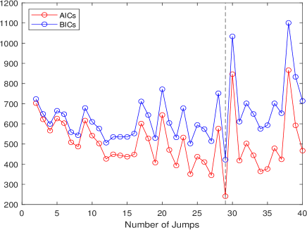
(a) AIC and BIC trends over the number of jumps.

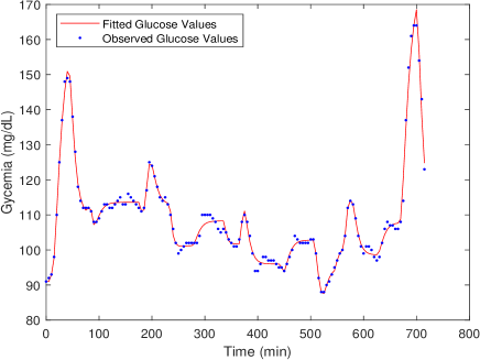
(b) Gycemia over time, $N_{Y}=29$.

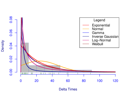
(c) Histogram of the Delta Times $(\Delta t_{i})_{i=1\ldots,N_{Y}-1}$.

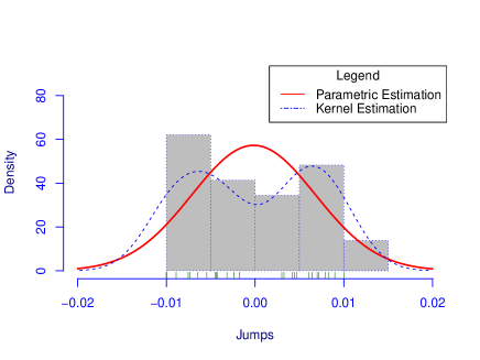
(d) Estimation of the density of the jumps values.

Figure 1: Results from Patient AA01.

Patient BO01

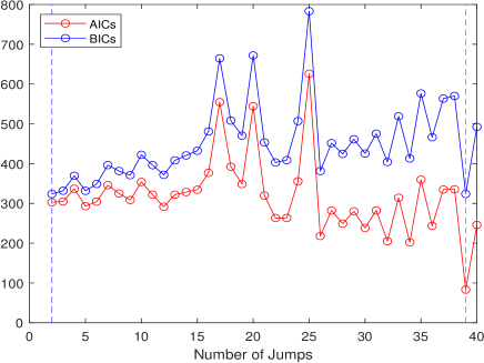
(a) AIC and BIC trends over the number of jumps.

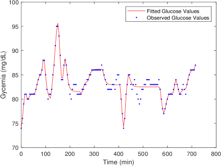
(b) Gycemia over time, $N_{Y}=39$.

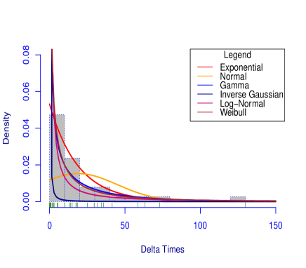
(c) Histogram of the Delta Times $(\Delta t_{i})_{i=1\ldots,N_{Y}-1}$.

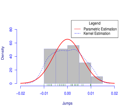
(d) Estimation of the density of the jumps values.

Figure 2: Results from Patient BO01.

Patient CI01

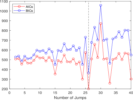
(a) AIC and BIC trends over the number of jumps.

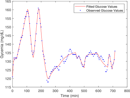
(b) Gycemia over time, $N_{Y}=26$

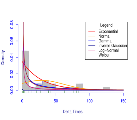
(c) Histogram of the Delta Times $(\Delta t_{i})_{i=1\ldots,N_{Y}-1}$.

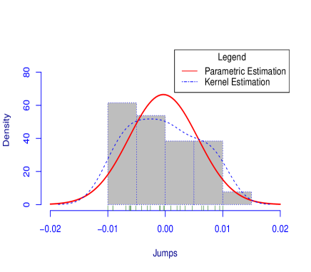
(d) Estimation of the density of the jumps values.

Figure 3: Results from Patient CI01.

Patient LM01

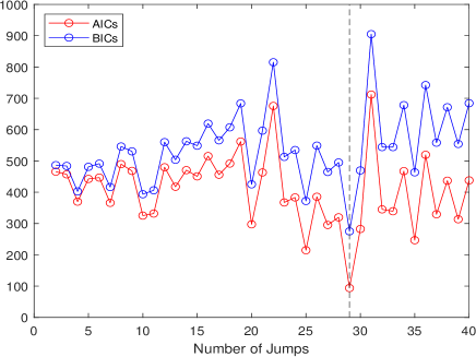
(a) AIC and BIC trends over the number of jumps.

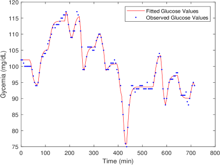
(b) Gycemia over time, $N_{Y}=29$.

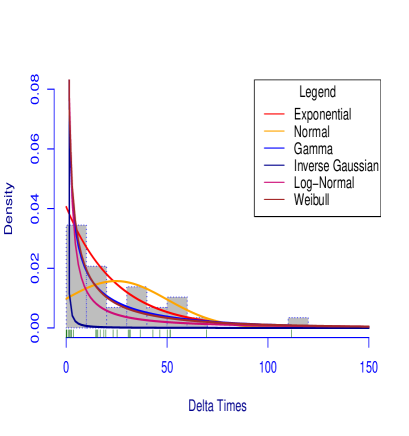
(c) Histogram of the Delta Times $(\Delta t_{i})_{i=1\ldots,N_{Y}-1}$.

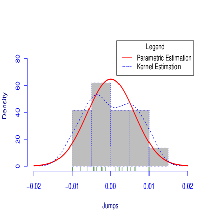
(d) Estimation of the density of the jumps values.

Figure 4: Results from Patient LM01.

Patient LR01

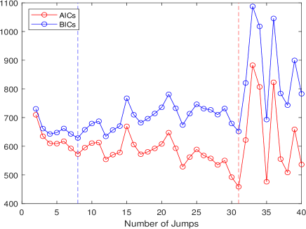
(a) AIC and BIC trends over the number of jumps.

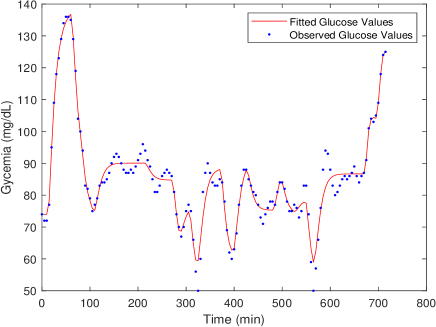
(b) Gycemia over time, $N_{Y}=31$.

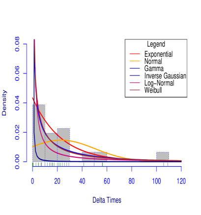
(c) Histogram of the Delta Times $(\Delta t_{i})_{i=1\ldots,N_{Y}-1}$.

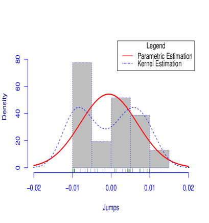
(d) Estimation of the density of the jumps values.

Figure 5: Results from Patient LR01.

Patient MA01

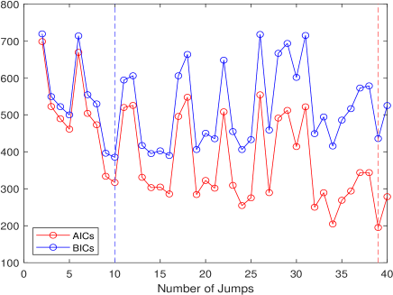
(a) AIC and BIC trends over the number of jumps.

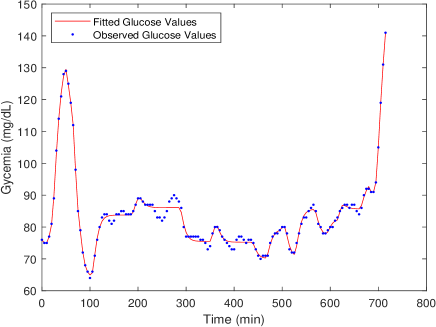
(b) Gycemia over time, $N_{Y}=39$.

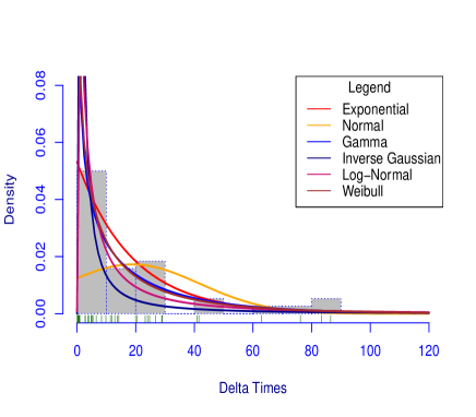
(c) Histogram of the Delta Times $(\Delta t_{i})_{i=1\ldots,N_{Y}-1}$.

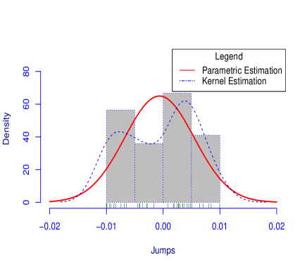
(d) Estimation of the density of the jumps values.

Figure 6: Results from Patient MA01.

Patient PS01

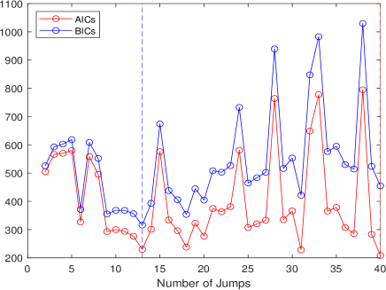
(a) AIC and BIC trends over the number of jumps.

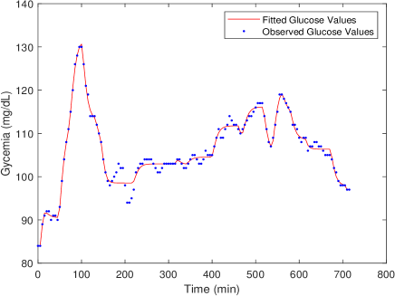
(b) Gycemia over time, $N_{Y}=40$.

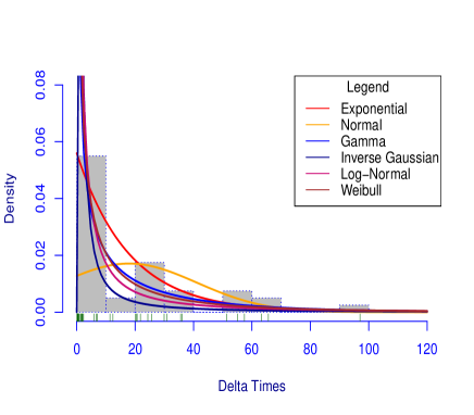
(c) Histogram of the Delta Times $(\Delta t_{i})_{i=1\ldots,N_{Y}-1}$.

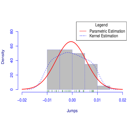
(d) Estimation of the density of the jumps values.

Figure 7: Results from Patient PS01.

Patient TO01

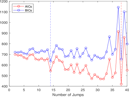
(a) AIC and BIC trends over the number of jumps.

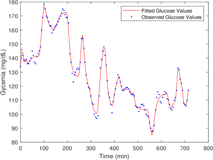
(b) Gycemia over time, $N_{Y}=38$.

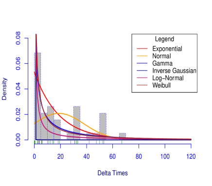
(c) Histogram of the Delta Times $(\Delta t_{i})_{i=1\ldots,N_{Y}-1}$.

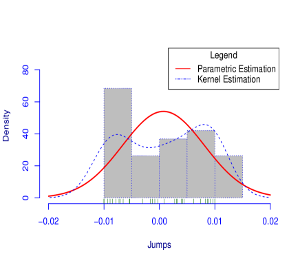
(d) Estimation of the density of the jumps values.

Figure 8: Results from Patient TO01.

Patient	Expectation $\mu$	Standard Deviation $\sigma$
AA01	-0.0001626885	0.006963786
BO01	-0.0000212980	0.006082102
CI01	-0.0003323163	0.005998925
LM01	0.00007391962	0.006144557
LR01	-0.0006154387	0.007353402
MA01	-0.0006552171	0.006140687
PS01	-0.0005062152	0.00602809
TO01	0.0007230374	0.007385183

Table 3: Means and the standard deviations obtained from the normal parametric density for each patient.

In order to assess which probability distribution was most suited to fit the waiting times, An analysis of the goodness of the fittings was performed. Specifically, a comparison between the Exponential, Gamma, Normal, Log-Normal, Weibull and Inverse Gaussian distributions was carried out.

Distribution	AIC
Exponential	244.62
Gamma	245.25
Weibull	245.77
Log-Normal	258.20
Normal	269.12
Inverse-Gaussian	327.99

Table 4: Goodness of fit $\Delta t_{i}$ Patient AA01

Distribution	AIC
Gamma	272.7566
Weibull	275.8100
Log-Normal	292.0124
Exponential	301.0369
Normal	359.7758
Inverse-Gaussian	474.6699

Table 5: Goodness of fit $\Delta t_{i}$ Patient B001

Distribution	AIC
Gamma	162.8705
Weibull	172.5374
Log-Normal	206.9017
Exponential	219.6703
Normal	249.8459
Inverse-Gaussian	922.6549

Table 6: Goodness of fit $\Delta t_{i}$ Patient CI01

Distribution	AIC
Gamma	226.6330
Weibull	231.8983
Exponential	245.8892
Log-Normal	248.5496
Normal	273.8758
Inverse-Gaussian	399.9703

Table 7: Goodness of fit $\Delta t_{i}$ Patient LM01

Distribution	AIC
Gamma	239.1154
Weibull	244.0272
Exponential	258.5743
Log-Normal	262.3403
Normal	296.7596
Inverse-Gaussian	410.8386

Table 8: Goodness of fit $\Delta t_{i}$ Patient LR01

Distribution	AIC
Gamma	295.4941
Weibull	295.7222
Exponential	301.0369
Log-Normal	301.4513
Inverse-Gaussian	326.3976
Normal	350.4726

Table 9: Goodness of fit $\Delta t_{i}$ Patient MA01

Distribution	AIC
Gamma	289.1986
Weibull	289.5733
Log-Normal	291.2840
Inverse-Gaussian	305.0637
Exponential	312.6722
Normal	369.4195

Table 10: Goodness of fit $\Delta t_{i}$ Patient PS01

Distribution	AIC
Gamma	249.02
Weibull	261.46
Log-Normal	296.82
Exponential	301.04
Normal	336.10
Inverse-Gaussian	741.39

Table 11: Goodness of fit $\Delta t_{i}$ Patient TO01

According to Tables 4, 5, 6, 7, 8, 9, 10, 11, the Gamma distribution appears to be the optimal one. We report in table 12, with the gamlss.family notation  [36], the corresponding estimated parameters through the Maximum Likelihood Estimation (MLE) method.

Patient	$N_{Y}$	$\mu$	$\sigma$
AA01	29	24.12264	1.136236
BO01	39	18.81577	1.563323
CI01	26	28.60001	1.971192
LM01	29	24.65488	1.540134
LR01	31	23.06438	1.524811
MA01	39	18.81577	1.279943
PS01	40	17.87475	1.503246
TO01	38	18.81579	1.753733

Table 12: Parameters of the Gamma Distribution estimated for each patient.

For the sake of completeness, the best fit of parameter values for each subject (according to the Akaike Information Criterion) is shown in tables 13, 14, 15, 16, 17, 18, 19,20, 21.

Patient	$\mathbf{N_{Y}}$	$\mathbf{k_{EH}}$	$\mathbf{H_{0}}$	$\mathbf{Y_{0}}$
H]||l|l|l|l|l|| AA01	29	1.5151577e-01	1.9999999e-01	-9.9972279e-01
BO01	39	1.9999963e-01	1.9999985e-01	9.9999921e-01
CI01	26	1.9999999e-01	2.0909944e-02	6.9208498e-01
LM01	29	1.9999996e-01	1.5973173e-01	-9.9999911e-01
LR01	31	1.6221208e-01	1.4979140e-01	-9.4417929e-01
MA01	39	1.9999997e-01	1.8175307e-01	-9.0751673e-02
PS01	40	1.9414967e-01	2.0000000e-01	-8.7246572e-01
TO01	38	1.0272332e-01	2.0000000e-01	-9.9980120e-01

Table 13: Kinetic parameters per patient according to the best number of Jumps $N_{Y}$.

$\mathbf{t_{1}}$	$\mathbf{t_{2}}$	$\mathbf{t_{3}}$	$\mathbf{t_{4}}$	$\mathbf{t_{5}}$
5.2364027	12.8370142	41.5858319	77.7234427	80.6372994
$\mathbf{Y_{1}}$	$\mathbf{Y_{2}}$	$\mathbf{Y_{3}}$	$\mathbf{Y_{4}}$	$\mathbf{Y_{5}}$
-0.0031786	-0.0099723	0.0078998	-0.0054477	0.0100000
$\mathbf{t_{6}}$	$\mathbf{t_{7}}$	$\mathbf{t_{8}}$	$\mathbf{t_{9}}$	$\mathbf{t_{10}}$
86.7001226	86.7120607	175.3760136	181.0414045	194.3757596
$\mathbf{Y_{6}}$	$\mathbf{Y_{7}}$	$\mathbf{Y_{8}}$	$\mathbf{Y_{9}}$	$\mathbf{Y_{10}}$
0.0046722	-0.0100000	0.0032524	-0.0075409	0.0044350
$\mathbf{t_{11}}$	$\mathbf{t_{12}}$	$\mathbf{t_{13}}$	$\mathbf{t_{14}}$	$\mathbf{t_{15}}$
232.3488651	236.7362091	277.0105840	335.8868838	338.5933877
$\mathbf{Y_{11}}$	$\mathbf{Y_{12}}$	$\mathbf{Y_{13}}$	$\mathbf{Y_{14}}$	$\mathbf{Y_{15}}$
0.0071978	-0.0043805	-0.0017729	0.0060891	-0.0044720
$\mathbf{t_{16}}$	$\mathbf{t_{17}}$	$\mathbf{t_{18}}$	$\mathbf{t_{19}}$	$\mathbf{t_{20}}$
364.7587451	370.7980945	443.1351053	445.5294229	505.5644604
$\mathbf{Y_{16}}$	$\mathbf{Y_{17}}$	$\mathbf{Y_{18}}$	$\mathbf{Y_{19}}$	$\mathbf{Y_{20}}$
-0.0073427	0.0089861	0.0069922	-0.0088973	0.0064212
$\mathbf{t_{21}}$	$\mathbf{t_{22}}$	$\mathbf{t_{23}}$	$\mathbf{t_{24}}$	$\mathbf{t_{25}}$
520.5688299	545.8138547	546.7999130	560.8694650	568.7932271
$\mathbf{Y_{21}}$	$\mathbf{Y_{22}}$	$\mathbf{Y_{23}}$	$\mathbf{Y_{24}}$	$\mathbf{Y_{25}}$
-0.0042245	-0.0100000	0.0083088	-0.0065152	0.0041529
$\mathbf{t_{26}}$	$\mathbf{t_{27}}$	$\mathbf{t_{28}}$	$\mathbf{t_{29}}$
578.0625743	626.2670384	668.4789765	699.5566696
$\mathbf{Y_{26}}$	$\mathbf{Y_{27}}$	$\mathbf{Y_{28}}$	$\mathbf{Y_{29}}$
0.0030111	-0.0023915	-0.0100000	0.0100000

Table 14: Patient AA01: Jump Times and Intensities of the Jumps , $N_{Y}$=29.

$\mathbf{t_{1}}$	$\mathbf{t_{2}}$	$\mathbf{t_{3}}$	$\mathbf{t_{4}}$	$\mathbf{t_{5}}$
1.7531642	6.9422950	9.6426214	14.9446212	15.2104916
$\mathbf{Y_{1}}$	$\mathbf{Y_{2}}$	$\mathbf{Y_{3}}$	$\mathbf{Y_{4}}$	$\mathbf{Y_{5}}$
-0.0077292	0.0099049	-0.0087262	0.0033857	0.0019620
$\mathbf{t_{6}}$	$\mathbf{t_{7}}$	$\mathbf{t_{8}}$	$\mathbf{t_{9}}$	$\mathbf{t_{10}}$
20.8367196	21.6261287	56.1390841	81.2205516	91.3284842
$\mathbf{Y_{6}}$	$\mathbf{Y_{7}}$	$\mathbf{Y_{8}}$	$\mathbf{Y_{9}}$	$\mathbf{Y_{10}}$
-0.0014224	-0.0009051	-0.0017687	-0.0023248	0.0046516
$\mathbf{t_{11}}$	$\mathbf{t_{12}}$	$\mathbf{t_{13}}$	$\mathbf{t_{14}}$	$\mathbf{t_{15}}$
120.9721043	121.8619375	132.0787944	150.5280246	150.7901859
$\mathbf{Y_{11}}$	$\mathbf{Y_{12}}$	$\mathbf{Y_{13}}$	$\mathbf{Y_{14}}$	$\mathbf{Y_{15}}$
-0.0079149	0.0042477	-0.0030421	-0.0034532	0.0098593
$\mathbf{t_{16}}$	$\mathbf{t_{17}}$	$\mathbf{t_{18}}$	$\mathbf{t_{19}}$	$\mathbf{t_{20}}$
165.8442276	179.0751796	242.4253110	243.5121682	273.0707517
$\mathbf{Y_{16}}$	$\mathbf{Y_{17}}$	$\mathbf{Y_{18}}$	$\mathbf{Y_{19}}$	$\mathbf{Y_{20}}$
-0.0041980	0.0037630	0.0043378	-0.0052634	-0.0071043
$\mathbf{t_{21}}$	$\mathbf{t_{22}}$	$\mathbf{t_{23}}$	$\mathbf{t_{24}}$	$\mathbf{t_{25}}$
273.3078462	332.0561503	405.1572658	405.2791883	420.2552715
$\mathbf{Y_{21}}$	$\mathbf{Y_{22}}$	$\mathbf{Y_{23}}$	$\mathbf{Y_{24}}$	$\mathbf{Y_{25}}$
0.0060889	0.0013333	0.0020822	0.0032244	-0.0069572
$\mathbf{t_{26}}$	$\mathbf{t_{27}}$	$\mathbf{t_{28}}$	$\mathbf{t_{29}}$
437.9785828	567.8344144	585.2840801	626.8542070	629.2681306
$\mathbf{Y_{26}}$	$\mathbf{Y_{27}}$	$\mathbf{Y_{28}}$	$\mathbf{Y_{29}}$	$\mathbf{Y_{30}}$
0.0018411	0.0029846	-0.0024690	-0.0067185	0.0066140
$\mathbf{t_{31}}$	$\mathbf{t_{32}}$	$\mathbf{t_{33}}$	$\mathbf{t_{34}}$	$\mathbf{t_{35}}$
643.2776360	643.9756707	675.6225995	711.4105311	711.6292886
$\mathbf{Y_{31}}$	$\mathbf{Y_{32}}$	$\mathbf{Y_{33}}$	$\mathbf{Y_{34}}$	$\mathbf{Y_{35}}$
0.0097737	-0.0100000	-0.0017152	-0.0082753	0.0066267
$\mathbf{t_{36}}$	$\mathbf{t_{37}}$	$\mathbf{t_{38}}$	$\mathbf{t_{39}}$
714.9978196	714.9998922	715.0000000	715.0000000
$\mathbf{Y_{36}}$	$\mathbf{Y_{37}}$	$\mathbf{Y_{38}}$	$\mathbf{Y_{39}}$
-0.0035245	0.0100000	-0.0099993	0.0099996

Table 15: Patient BO01: Jump Times and Intensities of the Jumps , $N_{Y}$=39.

$\mathbf{t_{1}}$	$\mathbf{t_{2}}$	$\mathbf{t_{3}}$	$\mathbf{t_{4}}$	$\mathbf{t_{5}}$
0.0000000	0.0000000	1.7661084	2.4728315	23.8122309
$\mathbf{Y_{1}}$	$\mathbf{Y_{2}}$	$\mathbf{Y_{3}}$	$\mathbf{Y_{4}}$	$\mathbf{Y_{5}}$
-0.0040950	-0.0068447	0.0074244	0.0034137	-0.0009755
$\mathbf{t_{6}}$	$\mathbf{t_{7}}$	$\mathbf{t_{8}}$	$\mathbf{t_{9}}$	$\mathbf{t_{10}}$
62.9555029	105.7246465	141.1139283	180.2594550	243.0826317
$\mathbf{Y_{6}}$	$\mathbf{Y_{7}}$	$\mathbf{Y_{8}}$	$\mathbf{Y_{9}}$	$\mathbf{Y_{10}}$
-0.0003314	0.0020335	-0.0025940	0.0025657	-0.0008888
$\mathbf{t_{11}}$	$\mathbf{t_{12}}$	$\mathbf{t_{13}}$	$\mathbf{t_{14}}$	$\mathbf{t_{15}}$
319.5023530	442.2855711	444.3017886	457.5395079	499.8336690
$\mathbf{Y_{11}}$	$\mathbf{Y_{12}}$	$\mathbf{Y_{13}}$	$\mathbf{Y_{14}}$	$\mathbf{Y_{15}}$
-0.0001726	0.0047068	-0.0051530	0.0009582	-0.0091218
$\mathbf{t_{16}}$	$\mathbf{t_{17}}$	$\mathbf{t_{18}}$	$\mathbf{t_{19}}$	$\mathbf{t_{20}}$
501.1904024	584.7252873	584.8950891	665.1868158	668.4435777
$\mathbf{Y_{16}}$	$\mathbf{Y_{17}}$	$\mathbf{Y_{18}}$	$\mathbf{Y_{19}}$	$\mathbf{Y_{20}}$
0.0086406	-0.0091392	0.0094690	-0.0059866	0.0067016
$\mathbf{t_{21}}$	$\mathbf{t_{22}}$	$\mathbf{t_{23}}$	$\mathbf{t_{24}}$	$\mathbf{t_{25}}$
695.5277727	698.3367440	705.1897997	714.8207471	714.9125837
$\mathbf{Y_{21}}$	$\mathbf{Y_{22}}$	$\mathbf{Y_{23}}$	$\mathbf{Y_{24}}$	$\mathbf{Y_{25}}$
-0.0062823	0.0063404	-0.0031597	-0.0100000	0.0099975
$\mathbf{t_{26}}$
714.9993925
$\mathbf{Y_{26}}$
-0.0061470

Table 16: Patient CI01: Jump Times and Intensities of the Jumps , $N_{Y}$=26.

$\mathbf{t_{1}}$	$\mathbf{t_{2}}$	$\mathbf{t_{3}}$	$\mathbf{t_{4}}$	$\mathbf{t_{5}}$
36.6884378	36.7057686	67.9336347	110.8990587	180.4096177
$\mathbf{Y_{1}}$	$\mathbf{Y_{2}}$	$\mathbf{Y_{3}}$	$\mathbf{Y_{4}}$	$\mathbf{Y_{5}}$
0.0051069	-0.0023904	-0.0036958	-0.0024041	-0.0044771
$\mathbf{t_{6}}$	$\mathbf{t_{7}}$	$\mathbf{t_{8}}$	$\mathbf{t_{9}}$	$\mathbf{t_{10}}$
183.9066619	209.1660485	240.9189356	256.0984147	302.4857421
$\mathbf{Y_{6}}$	$\mathbf{Y_{7}}$	$\mathbf{Y_{8}}$	$\mathbf{Y_{9}}$	$\mathbf{Y_{10}}$
0.0061199	-0.0020663	0.0064213	-0.0038317	-0.0013097
$\mathbf{t_{11}}$	$\mathbf{t_{12}}$	$\mathbf{t_{13}}$	$\mathbf{t_{14}}$	$\mathbf{t_{15}}$
325.7139632	341.3859477	342.5575031	345.2138864	345.2910954
$\mathbf{Y_{11}}$	$\mathbf{Y_{12}}$	$\mathbf{Y_{13}}$	$\mathbf{Y_{14}}$	$\mathbf{Y_{15}}$
0.0022173	0.0099747	-0.0060372	-0.0044706	0.0012415
$\mathbf{t_{16}}$	$\mathbf{t_{17}}$	$\mathbf{t_{18}}$	$\mathbf{t_{19}}$	$\mathbf{t_{20}}$
396.8162060	415.4458159	432.3201529	544.0285164	544.0408002
$\mathbf{Y_{16}}$	$\mathbf{Y_{17}}$	$\mathbf{Y_{18}}$	$\mathbf{Y_{19}}$	$\mathbf{Y_{20}}$
0.0042504	0.0082136	-0.0100000	-0.0077589	0.0043591
$\mathbf{t_{21}}$	$\mathbf{t_{22}}$	$\mathbf{t_{23}}$	$\mathbf{t_{24}}$	$\mathbf{t_{25}}$
574.7776621	594.4572234	644.5672747	696.0315707	698.2948359
$\mathbf{Y_{21}}$	$\mathbf{Y_{22}}$	$\mathbf{Y_{23}}$	$\mathbf{Y_{24}}$	$\mathbf{Y_{25}}$
0.0062931	-0.0041780	0.0026677	-0.0051616	0.0029556
$\mathbf{t_{26}}$	$\mathbf{t_{27}}$	$\mathbf{t_{28}}$	$\mathbf{t_{29}}$
712.9636084	714.6250258	714.9998962	714.9999976
$\mathbf{Y_{26}}$	$\mathbf{Y_{27}}$	$\mathbf{Y_{28}}$	$\mathbf{Y_{29}}$
0.0100000	-0.0099142	0.0099959	-0.0099779

Table 17: Patient LM01: Jump Times and Intensities of the Jumps , $N_{Y}$=29.

$\mathbf{t_{1}}$	$\mathbf{t_{2}}$	$\mathbf{t_{3}}$	$\mathbf{t_{4}}$	$\mathbf{t_{5}}$
11.9094990	12.1019352	18.8857897	60.1995371	80.3116479
$\mathbf{Y_{1}}$	$\mathbf{Y_{2}}$	$\mathbf{Y_{3}}$	$\mathbf{Y_{4}}$	$\mathbf{Y_{5}}$
-0.0095361	-0.0067635	0.0049676	0.0072610	0.0037596
$\mathbf{t_{6}}$	$\mathbf{t_{7}}$	$\mathbf{t_{8}}$	$\mathbf{t_{9}}$	$\mathbf{t_{10}}$
102.6433724	105.3788574	214.4145746	270.8216896	284.8259552
$\mathbf{Y_{6}}$	$\mathbf{Y_{7}}$	$\mathbf{Y_{8}}$	$\mathbf{Y_{9}}$	$\mathbf{Y_{10}}$
0.0055537	-0.0095769	0.0012560	0.0075091	-0.0054062
$\mathbf{t_{11}}$	$\mathbf{t_{12}}$	$\mathbf{t_{13}}$	$\mathbf{t_{14}}$	$\mathbf{t_{15}}$
306.1164378	321.7760341	321.7802714	371.5177862	397.2661914
$\mathbf{Y_{11}}$	$\mathbf{Y_{12}}$	$\mathbf{Y_{13}}$	$\mathbf{Y_{14}}$	$\mathbf{Y_{15}}$
0.0100000	-0.0094967	-0.0034873	0.0093145	-0.0100000
$\mathbf{t_{16}}$	$\mathbf{t_{17}}$	$\mathbf{t_{18}}$	$\mathbf{t_{19}}$	$\mathbf{t_{20}}$
424.8279178	481.1300941	495.1351204	524.4073781	524.4973720
$\mathbf{Y_{16}}$	$\mathbf{Y_{17}}$	$\mathbf{Y_{18}}$	$\mathbf{Y_{19}}$	$\mathbf{Y_{20}}$
0.0042316	-0.0041911	0.0045482	0.0084638	-0.0098451
$\mathbf{t_{21}}$	$\mathbf{t_{22}}$	$\mathbf{t_{23}}$	$\mathbf{t_{24}}$	$\mathbf{t_{25}}$
548.5406082	564.6585589	564.6706719	670.4498730	677.6272855
$\mathbf{Y_{21}}$	$\mathbf{Y_{22}}$	$\mathbf{Y_{23}}$	$\mathbf{Y_{24}}$	$\mathbf{Y_{25}}$
0.0100000	-0.0100000	-0.0021187	-0.0080012	0.0047936
$\mathbf{t_{26}}$	$\mathbf{t_{27}}$	$\mathbf{t_{28}}$	$\mathbf{t_{29}}$	$\mathbf{t_{30}}$
695.0151092	704.9939567	709.7015756	714.4760969	714.9998480
$\mathbf{Y_{26}}$	$\mathbf{Y_{27}}$	$\mathbf{Y_{28}}$	$\mathbf{Y_{29}}$	$\mathbf{Y_{30}}$
-0.0060884	0.0029632	0.0009097	-0.0100000	-0.0100000
$\mathbf{t_{31}}$
715.0000000
$\mathbf{Y_{31}}$
0.0099010

Table 18: Patient LR01: Jump Times and Intensities of the Jumps , $N_{Y}$=31.

$\mathbf{t_{1}}$	$\mathbf{t_{2}}$	$\mathbf{t_{3}}$	$\mathbf{t_{4}}$	$\mathbf{t_{5}}$
0.0000000	0.9343427	1.5716458	6.4013948	7.1811615
$\mathbf{Y_{1}}$	$\mathbf{Y_{2}}$	$\mathbf{Y_{3}}$	$\mathbf{Y_{4}}$	$\mathbf{Y_{5}}$
0.0047970	-0.0092341	0.0070317	-0.0074344	0.0027602
$\mathbf{t_{6}}$	$\mathbf{t_{7}}$	$\mathbf{t_{8}}$	$\mathbf{t_{9}}$	$\mathbf{t_{10}}$
15.5114491	16.0585447	21.0411272	47.7576120	60.6339624
$\mathbf{Y_{6}}$	$\mathbf{Y_{7}}$	$\mathbf{Y_{8}}$	$\mathbf{Y_{9}}$	$\mathbf{Y_{10}}$
0.0008573	-0.0064724	-0.0084104	0.0050180	0.0042248
$\mathbf{t_{11}}$	$\mathbf{t_{12}}$	$\mathbf{t_{13}}$	$\mathbf{t_{14}}$	$\mathbf{t_{15}}$
64.6421588	78.8809002	102.9121057	186.3817151	200.1306431
$\mathbf{Y_{11}}$	$\mathbf{Y_{12}}$	$\mathbf{Y_{13}}$	$\mathbf{Y_{14}}$	$\mathbf{Y_{15}}$
0.0084626	0.0050318	-0.0100000	-0.0027989	0.0019029
$\mathbf{t_{16}}$	$\mathbf{t_{17}}$	$\mathbf{t_{18}}$	$\mathbf{t_{19}}$	$\mathbf{t_{20}}$
286.6105518	349.5966979	360.9874552	437.1483624	466.2192794
$\mathbf{Y_{16}}$	$\mathbf{Y_{17}}$	$\mathbf{Y_{18}}$	$\mathbf{Y_{19}}$	$\mathbf{Y_{20}}$
0.0045002	-0.0036133	0.0037398	0.0026732	-0.0045150
$\mathbf{t_{21}}$	$\mathbf{t_{22}}$	$\mathbf{t_{23}}$	$\mathbf{t_{24}}$	$\mathbf{t_{25}}$
495.0856241	501.6031208	505.3289708	525.2767625	566.7834641
$\mathbf{Y_{21}}$	$\mathbf{Y_{22}}$	$\mathbf{Y_{23}}$	$\mathbf{Y_{24}}$	$\mathbf{Y_{25}}$
-0.0016203	0.0034584	0.0024203	-0.0068581	0.0034836
$\mathbf{t_{26}}$	$\mathbf{t_{27}}$	$\mathbf{t_{28}}$	$\mathbf{t_{29}}$	$\mathbf{t_{30}}$
590.0375421	590.4073183	615.1350938	620.5399033	661.3956095
$\mathbf{Y_{26}}$	$\mathbf{Y_{27}}$	$\mathbf{Y_{28}}$	$\mathbf{Y_{29}}$	$\mathbf{Y_{30}}$
0.0017887	-0.0040903	-0.0042061	0.0029953	-0.0029417
$\mathbf{t_{31}}$	$\mathbf{t_{32}}$	$\mathbf{t_{33}}$	$\mathbf{t_{34}}$	$\mathbf{t_{35}}$
681.9175802	684.6887691	694.5082016	706.3630122	706.9024544
$\mathbf{Y_{31}}$	$\mathbf{Y_{32}}$	$\mathbf{Y_{33}}$	$\mathbf{Y_{34}}$	$\mathbf{Y_{35}}$
0.0080239	-0.0098925	-0.0099999	0.0064575	-0.0086679
$\mathbf{t_{36}}$	$\mathbf{t_{37}}$	$\mathbf{t_{38}}$	$\mathbf{t_{39}}$
711.9234096	714.7543400	714.8149993	714.9997922
$\mathbf{Y_{36}}$	$\mathbf{Y_{37}}$	$\mathbf{Y_{38}}$	$\mathbf{Y_{39}}$
0.0050297	-0.0099854	-0.0094313	0.0099623

Table 19: Patient MA01: Jump Times and Intensities of the Jumps , $N_{Y}$=39.

$\mathbf{t_{1}}$	$\mathbf{t_{2}}$	$\mathbf{t_{3}}$	$\mathbf{t_{4}}$	$\mathbf{t_{5}}$
2.0113565	2.3088969	4.1534739	10.1520456	10.2058897
$\mathbf{Y_{1}}$	$\mathbf{Y_{2}}$	$\mathbf{Y_{3}}$	$\mathbf{Y_{4}}$	$\mathbf{Y_{5}}$
-0.0063838	0.0084358	-0.0093116	0.0076411	-0.0008623
$\mathbf{t_{6}}$	$\mathbf{t_{7}}$	$\mathbf{t_{8}}$	$\mathbf{t_{9}}$	$\mathbf{t_{10}}$
10.7173183	46.7399868	66.7684030	73.3555192	98.9393779
$\mathbf{Y_{6}}$	$\mathbf{Y_{7}}$	$\mathbf{Y_{8}}$	$\mathbf{Y_{9}}$	$\mathbf{Y_{10}}$
-0.0023263	-0.0068971	-0.0025987	-0.0018733	0.0080688
$\mathbf{t_{11}}$	$\mathbf{t_{12}}$	$\mathbf{t_{13}}$	$\mathbf{t_{14}}$	$\mathbf{t_{15}}$
99.0424512	129.7995020	142.1732497	153.5438316	153.9491208
$\mathbf{Y_{11}}$	$\mathbf{Y_{12}}$	$\mathbf{Y_{13}}$	$\mathbf{Y_{14}}$	$\mathbf{Y_{15}}$
-0.0038734	0.0015776	0.0029459	0.0029387	-0.0032109
$\mathbf{t_{16}}$	$\mathbf{t_{17}}$	$\mathbf{t_{18}}$	$\mathbf{t_{19}}$	$\mathbf{t_{20}}$
217.2682619	314.2622616	314.7854875	339.1542947	396.5938342
$\mathbf{Y_{16}}$	$\mathbf{Y_{17}}$	$\mathbf{Y_{18}}$	$\mathbf{Y_{19}}$	$\mathbf{Y_{20}}$
-0.0014188	-0.0078609	0.0079105	-0.0005204	0.0042779
$\mathbf{t_{21}}$	$\mathbf{t_{22}}$	$\mathbf{t_{23}}$	$\mathbf{t_{24}}$	$\mathbf{t_{25}}$
397.0592501	462.6756865	464.1050900	515.4325426	536.1261318
$\mathbf{Y_{21}}$	$\mathbf{Y_{22}}$	$\mathbf{Y_{23}}$	$\mathbf{Y_{24}}$	$\mathbf{Y_{25}}$
-0.0063021	0.0082240	-0.0093226	0.0028341	-0.0039921
$\mathbf{t_{26}}$	$\mathbf{t_{27}}$	$\mathbf{t_{28}}$	$\mathbf{t_{29}}$	$\mathbf{t_{30}}$
557.9196158	578.4245305	578.5709511	614.1591499	615.0693980
$\mathbf{Y_{26}}$	$\mathbf{Y_{27}}$	$\mathbf{Y_{28}}$	$\mathbf{Y_{29}}$	$\mathbf{Y_{30}}$
0.0015155	0.0070801	-0.0055078	0.0044835	-0.0038320
$\mathbf{t_{31}}$	$\mathbf{t_{32}}$	$\mathbf{t_{33}}$	$\mathbf{t_{34}}$	$\mathbf{t_{35}}$
670.2118978	700.1335297	702.4794698	703.4086819	705.1864281
$\mathbf{Y_{31}}$	$\mathbf{Y_{32}}$	$\mathbf{Y_{33}}$	$\mathbf{Y_{34}}$	$\mathbf{Y_{35}}$
0.0026162	-0.0012974	0.0084021	-0.0097769	0.0046276
$\mathbf{t_{36}}$	$\mathbf{t_{37}}$	$\mathbf{t_{38}}$	$\mathbf{t_{39}}$	$\mathbf{t_{40}}$
712.2488239	712.4516812	714.1077618	714.7089113	714.9999888
$\mathbf{Y_{36}}$	$\mathbf{Y_{37}}$	$\mathbf{Y_{38}}$	$\mathbf{Y_{39}}$	$\mathbf{Y_{40}}$
0.0009019	-0.0081884	-0.0100000	0.0099993	-0.0093725

Table 20: Patient PS01: Jump Times and Intensities of the Jumps , $N_{Y}$=40.

$\mathbf{t_{1}}$	$\mathbf{t_{2}}$	$\mathbf{t_{3}}$	$\mathbf{t_{4}}$	$\mathbf{t_{5}}$
0.0000000	0.0001144	0.0105762	3.2892763	3.5840276
$\mathbf{Y_{1}}$	$\mathbf{Y_{2}}$	$\mathbf{Y_{3}}$	$\mathbf{Y_{4}}$	$\mathbf{Y_{5}}$
-0.0100000	-0.0016208	-0.0002454	0.0100000	0.0041683
$\mathbf{t_{6}}$	$\mathbf{t_{7}}$	$\mathbf{t_{8}}$	$\mathbf{t_{9}}$	$\mathbf{t_{10}}$
14.7586344	20.1801000	26.2047859	79.4419142	97.7874796
$\mathbf{Y_{6}}$	$\mathbf{Y_{7}}$	$\mathbf{Y_{8}}$	$\mathbf{Y_{9}}$	$\mathbf{Y_{10}}$
-0.0065450	0.0061877	-0.0030495	-0.0054302	0.0032026
$\mathbf{t_{11}}$	$\mathbf{t_{12}}$	$\mathbf{t_{13}}$	$\mathbf{t_{14}}$	$\mathbf{t_{15}}$
145.2549962	197.4705932	197.5688561	247.5807702	261.5608754
$\mathbf{Y_{11}}$	$\mathbf{Y_{12}}$	$\mathbf{Y_{13}}$	$\mathbf{Y_{14}}$	$\mathbf{Y_{15}}$
-0.0012758	0.0030801	0.0027528	-0.0072852	0.0091927
$\mathbf{t_{16}}$	$\mathbf{t_{17}}$	$\mathbf{t_{18}}$	$\mathbf{t_{19}}$	$\mathbf{t_{20}}$
293.4605883	326.2834112	357.2401251	390.6000889	421.5138176
$\mathbf{Y_{16}}$	$\mathbf{Y_{17}}$	$\mathbf{Y_{18}}$	$\mathbf{Y_{19}}$	$\mathbf{Y_{20}}$
0.0039706	-0.0100000	0.0088787	-0.0053374	0.0099990
$\mathbf{t_{21}}$	$\mathbf{t_{22}}$	$\mathbf{t_{23}}$	$\mathbf{t_{24}}$	$\mathbf{t_{25}}$
423.9835398	465.8993583	471.8250029	475.8807161	488.3437979
$\mathbf{Y_{21}}$	$\mathbf{Y_{22}}$	$\mathbf{Y_{23}}$	$\mathbf{Y_{24}}$	$\mathbf{Y_{25}}$
-0.0078473	0.0044494	-0.0100000	0.0096852	-0.0008359
$\mathbf{t_{26}}$	$\mathbf{t_{27}}$	$\mathbf{t_{28}}$	$\mathbf{t_{29}}$	$\mathbf{t_{30}}$
541.6525438	559.9605806	627.0197775	631.1670931	659.0129388
$\mathbf{Y_{26}}$	$\mathbf{Y_{27}}$	$\mathbf{Y_{28}}$	$\mathbf{Y_{29}}$	$\mathbf{Y_{30}}$
0.0073907	-0.0100000	0.0100000	-0.0089003	-0.0093494
$\mathbf{t_{31}}$	$\mathbf{t_{32}}$	$\mathbf{t_{33}}$	$\mathbf{t_{34}}$	$\mathbf{t_{35}}$
669.0283123	688.2858345	691.7415747	706.6907198	712.1671379
$\mathbf{Y_{31}}$	$\mathbf{Y_{32}}$	$\mathbf{Y_{33}}$	$\mathbf{Y_{34}}$	$\mathbf{Y_{35}}$
0.0086358	0.0083106	-0.0070506	-0.0084924	0.0099757
$\mathbf{t_{36}}$	$\mathbf{t_{37}}$	$\mathbf{t_{38}}$
712.8397024	714.9999999	715.0000000
$\mathbf{Y_{36}}$	$\mathbf{Y_{37}}$	$\mathbf{Y_{38}}$
0.0008613	0.0100000	0.0099997

Table 21: Patient TO01: Jump Times and Intensities of the Jumps , $N_{Y}$=38.

4 Discussion

In the present work a simple ODE model of night-time CGM data has been devised for each of eight experimental T2DM subjects with good metabolic control. It is clear that this work does not have any pretense of generality: rather, it endeavors to provide a proof of concept showing that the explicit representation of stochastic jumps allows the experimenter to interpret a noisy CGM signal without necessarily refer to a diet and exercise diary kept by the patient. Indeed, such diaries have been proven to be cumbersome to keep and of very limited value in the interpretation of the time course of glycemia, due to frequent omission of relevant events and due to the unavoidable imprecision in quantifying food intake and exercise levels. In addition, the (meta-)parameters estimated on the samples of waiting times and on the sample of jump intensities, together with such directly interpretable kinetic parameters such as $k_{G}$, may represent a first-line assessment of the status of the subject. These (meta-)parameters are easy to obtain repeatedly on non-invasive CGM tracings and could be useful in following a subject’s clinical course. Routine, automated incorporation of the model within glycemia-tracking software apps may help to continuously monitor the state of health of a patient at no extra cost and with no added invasiveness.

Declaration of Interests

None

Fundings

This research did not receive any specific grant from funding agencies in the public, commercial, or not-for-profit sectors.

Credit authorship contribution statement

Giulia Elena Aliffi: Conceptualization, Methodology, Software, Formal Analysis, Investigation, Writing-original draft, Writing-review & editing. Giovanni Nastasi: Methodology, Writing-review & editing. Vittorio Romano: Methodology, Formal Analysis, Writing-review & editing, Supervision, Project Administration. Dario Pitocco: Resources, Data curation, Writing-review & editing. Alessandro Rizzi: Resources, Data curation, Writing-review & editing. Elvin J. Moore: Methodology, Formal Analysis, Writing-review & editing. Andrea De Gaetano: Conceptualization, Methodology, Writing-review & editing, Supervision.

All authors have read and agreed to the published version of the manuscript.

References

- [1] Alam S, Hasan MK, Neaz S, Hussain N, Hossain MF, Rahman T. Diabetes Mellitus: Insights from Epidemiology, Biochemistry, Risk Factors, Diagnosis, Complications and Comprehensive Management. Diabetology. 2021; 2(2):36-50. https://doi.org/10.3390/diabetology2020004.
- [2] World Health Organizatin (WHO. Global Report on Diabetes; WHO: Geneva, Switzerlan, 2017. Avaible online:http://www.who.int/diabetes/global-report/en.
- [3] Kharroubi AT, Darwish HM. Diabetes mellitus: The epidemic of the century. World J Diabetes. 2015;6(6):850-867. doi:10.4239/wjd.v6.i6.850.
- [4] Rafique I, Mir A, Saqib MAN, Naeem M, Marchand L, Polychronakos C. Causal variants in Maturity Onset Diabetes of the Young (MODY) - A systematic review. BMC Endocr Disord. 2021 Nov 11;21(1):223. doi: 10.1186/s12902-021-00891-7. PMID: 34763692; PMCID: PMC8582101.
- [5] Thanabalasingham G, Owen KR. Diagnosis and management of maturity onset diabetes of the young (MODY). BMJ. 2011 Oct 19;343:d6044. doi: 10.1136/bmj.d6044. PMID: 22012810.
- [6] Dovč K, Bratina N, Battelino T. A new horizon for glucose monitoring. Horm Res Paediatr. 2015;83(3):149-56. doi: 10.1159/000368924. Epub 2015 Feb 5. PMID: 25660230.
- [7] National Institute of Diabetes and Digestive and Kidney Diseases. Continuous Glucose Monitoring. Available from: https://www.niddk.nih.gov/health-information/diabetes/overview/managing-diabetes/continuous-glucose-monitoring.
- [8] Rodbard D. Continuous Glucose Monitoring: A Review of Successes, Challenges, and Opportunities. Diabetes Technol Ther. 2016 Feb;18 Suppl 2(Suppl 2):S3-S13. doi: 10.1089/dia.2015.0417. PMID: 26784127; PMCID: PMC4717493.
- [9] Huard B, Kirkham G. Mathematical modelling of glucose dynamics, Current Opinion in Endocrine and Metabolic Research, Volume 25, 2022, 100379, ISSN 2451-9650, https://doi.org/10.1016/j.coemr.2022.100379.
- [10] Palumbo P, Ditlevsen S, Bertuzzi A, De Gaetano A. Mathematical modeling of the glucose-insulin system: a review. Math Biosci. 2013 Aug;244(2):69-81. doi: 10.1016/j.mbs.2013.05.006. Epub 2013 Jun 1. PMID: 23733079.
- [11] De Gaetano A, Arino O. Mathematical modelling of the intravenous glucose tolerance test. J Math Biol. 2000 Feb;40(2):136-68. doi: 10.1007/s002850050007. PMID: 10743599.
- [12] Panunzi S, Palumbo P, De Gaetano A. A discrete Single Delay Model for the Intra-Venous Glucose Tolerance Test. Theor Biol Med Model. 2007 Sep 12;4:35. doi: 10.1186/1742-4682-4-35. PMID: 17850652; PMCID: PMC2072949.
- [13] Pacini G, Bergman RN. MINMOD: a computer program to calculate insulin sensitivity and pancreatic responsivity from the frequently sampled intravenous glucose tolerance test. Comput Methods Programs Biomed. 1986 Oct;23(2):113-22. doi: 10.1016/0169-2607(86)90106-9. PMID: 3640682.
- [14] Bergman RN, Ider YZ, Bowden CR, Cobelli C. Quantitative estimation of insulin sensitivity. Am J Physiol. 1979 Jun;236(6):E667-77. doi: 10.1152/ajpendo.1979.236.6.E667. PMID: 443421.
- [15] Boston RC, Stefanovski D, Moate PJ, Sumner AE, Watanabe RM, Bergman RN. MINMOD Millennium: a computer program to calculate glucose effectiveness and insulin sensitivity from the frequently sampled intravenous glucose tolerance test. Diabetes Technol Ther. 2003;5(6):1003-15. doi: 10.1089/152091503322641060. PMID: 14709204.
- [16] Cho Y, Kim I, Sheen D. A fractional-order model for MINMOD Millennium, Mathematical Biosciences, Volume 262, 2015, Pages 36-45, ISSN 0025-5564, https://doi.org/10.1016/j.mbs.2014.11.008.
- [17] Coman S, Boldisor C, Floroian L. Fractional adaptive control for a fractional - order insuline - glucose dynamic model, 2017 International Conference on Optimization of Electrical and Electronic Equipment (OPTIM) & 2017 Intl Aegean Conference on Electrical Machines and Power Electronics (ACEMP), 2017, pp. 887-892, doi: 10.1109/OPTIM.2017.7975082.
- [18] Rooka S, Ghasemi R. Designing Fractional Ts Observers For A Class Of Fractional Model Of The Blood Glucose For Type I Diabetes, International Journal of Advances in Science, Engineering and Technology(IJASEAT) 2015, pp. 116-123, Volume-3, issue-4, Spl. Iss-3. Available from: http://www.iraj.in/journal/journal_file/journal_pdf/6-205-1449213837116-123.pdf
- [19] Pompa M, Panunzi S, Borri A, De Gaetano A. A comparison among three maximal mathematical models of the glucose-insulin system. PLoS One. 2021 Sep 27;16(9):e0257789. doi: 10.1371/journal.pone.0257789. PMID: 34570804; PMCID: PMC8476045.
- [20] Boiroux D, Hagdrup M, Mahmoudi Z, Poulsen NK, Madsen H, Jørgensen JB. Model Identification using Continuous Glucose Monitoring Data for Type 1 Diabetes**This work has been funded by the Danish Diabetes Academy supported by the Novo Nordisk Foundation., IFAC-PapersOnLine, Volume 49, Issue 7, 2016, Pages 759-764, ISSN 2405-8963, https://doi.org/10.1016/j.ifacol.2016.07.279.
- [21] Kanderian SS, Weinzimer S, Voskanyan G, Steil GM. Identification of intraday metabolic profiles during closed-loop glucose control in individuals with type 1 diabetes. J Diabetes Sci Technol. 2009 Sep 1;3(5):1047-57. doi: 10.1177/193229680900300508. PMID: 20144418; PMCID: PMC2769900.
- [22] Palumbo P, De Gaetano A. (2007). State Feedback Control of the Glucose-Insulin System. In: Aletti G., Micheletti A., Morale D., Burger M. (eds) Math Everywhere. Springer, Berlin, Heidelberg. https://doi.org/10.1007/978-3-540-44446-620
- [23] Panunzi S, De Gaetano A, Mingrone G. Advantages of the single delay model for the assessment of insulin sensitivity from the intravenous glucose tolerance test. Theor Biol Med Model. 2010 Mar 18;7:9. doi: 10.1186/1742-4682-7-9. PMID: 20298586; PMCID: PMC2858103.
- [24] Saleem MU, Farman M, Ahmad A, Haque EU, Ahmad MO, A Caputo-Fabrizio fractional order model for control of glucose in insulin therapies for diabetes, Ain Shams Engineering Journal, Volume 11, Issue 4, 2020, Pages 1309-1316, ISSN 2090-4479, https://doi.org/10.1016/j.asej.2020.03.006.
- [25] De Gaetano A, Sakulrang S, Borri A, Pitocco D, Sungnul S, Moore EJ. Modeling continuous glucose monitoring with fractional differential equations subject to shocks. J Theor Biol. 2021 Oct 7;526:110776. doi: 10.1016/j.jtbi.2021.110776. Epub 2021 May 28. PMID: 34058226.
- [26] De Gaetano A, Panunzi S, Matone A, Samson A, Vrbikova J, Bendlova B, Pacini G. Routine OGTT: a robust model including incretin effect for precise identification of insulin sensitivity and secretion in a single individual. PLoS One. 2013 Aug 29;8(8):e70875. doi: 10.1371/journal.pone.0070875. PMID: 24009656; PMCID: PMC3756988.
- [27] Sakulrang S, Moore EJ, Sungnul S, De Gaetano A. A fractional differential equation model for continuous glucose monitoring data. Adv Differ Equ 2017, 150 (2017). https://doi.org/10.1186/s13662-017-1207-1
- [28] MATLAB. (2018). 9.7.0.1216025 (R2019b). Natick, Massachusetts: The MathWorks Inc.
- [29] R Core Team (2020). R: A language and environment for statistical computing. R Foundation for Statistical Computing, Vienna, Austria. URL https://www.R-project.org/.
- [30] Bozdogan, H. Model selection and Akaike’s Information Criterion (AIC): The general theory and its analytical extensions. Psychometrika 52, 345-370 (1987). https://doi.org/10.1007/BF02294361
- [31] Kennedy J, Eberhart R. Particle swarm optimization, Proceedings of ICNN’95 - International Conference on Neural Networks, 1995, pp. 1942-1948 vol.4, doi: 10.1109/ICNN.1995.488968.
- [32] Mezura-Montes E, Carlos A. Coello Coello, Constraint-handling in nature-inspired numerical optimization: Past, present and future, Swarm and Evolutionary Computation, Volume 1, Issue 4, 2011, Pages 173-194, ISSN 2210-6502, https://doi.org/10.1016/j.swevo.2011.10.001.
- [33] Pedersen ME. Good Parameters for Particle Swarm Optimization. Luxembourg: Hvass Laboratories, 2010. Available from: https://www.researchgate.net/profile/Mohamed_Mourad_Lafifi/post/Which-is-the-best-swarm-size-in-PSO/attachment/5b5b6f85b53d2f89289c14e1/AS%3A653084896288769%401532718981208/download/GoodParametersforParticleSwarmOptimization.pdf
- [34] Schwarz G. Estimating the Dimension of a Model. Ann. Statist. 6 (2) 461 - 464, March, 1978. https://doi.org/10.1214/aos/1176344136
- [35] Wit, E, van den Heuvel E, Romeijn J-W. All models are wrong…’: an introduction to model uncertainty. Statistica Neerlandica, 2012, 66(3), 217-236. https://doi.org/10.1111/j.1467-9574.2012.00530.x
- [36] Rigby RA, Stasinopoulos DM (2005). Generalized additive models for location, scale and shape,(with discussion). Applied Statistics, 2005, 54, 507-554. https://doi.org/10.1111/j.1467-9876.2005.00510.x
- [37] Silverman, B W. Density Estimation for Statistics and Data Analysis, 1986. Chapman & Hall, London http://dx.doi.org/10.1007/978-1-4899-3324-9