Control and safe continual learning of output-constrained nonlinear systems

Abstract

We propose a novel learning-based tracking controller for nonlinear systems of arbitrary relative degree. Here, we use sample-and-hold input signals and derive a bound on the required sampling frequency. While the controller guarantees tracking within prescribed, possibly time-varying bounds on the error signal, system data is collected at runtime to continuously improve the controller performance. Furthermore, a safe region is defined, in which the control signal can even be used to (persistently) excite the system and, thus, to enhance the learning outcome. A particular strength is the flexibility to incorporate different learning paradigms, e.g., reinforcement learning or non-parametric predictive controllers based on Willems et al.’s so-called fundamental lemma, which is demonstrated by numerical simulations.

[label_tuilm]organization=Technische Universität Ilmenau, Institute of Mathematics, Optimization-based Control Group,city=Ilmenau, country=Germany

[label_upb]organization=Universität Paderborn, Institut für Mathematik,city=Paderborn, country=Germany

[label_rug]organization=University of Groningen, Bernoulli Institute for Mathematics, Computer Science, and Artificial Intelligence,city=Groningen, country=The Netherlands [label_itu]organization=Istanbul Technical University, Department of Control and Automation Engineering,city=Istanbul, country=Turkey

1 Introduction

In the rapidly evolving field of control systems, the growing complexity and the deluge of collected data have given rise to an increasing application of data-driven approaches and learning techniques. While learning-based controllers often exhibit superior performance compared to classical designs, their applicability in safety-critical domains such as medical applications and human-robot interaction is impeded by a critical deficiency in ensuring rigorous constraint satisfaction, see e.g. [1]. We refer to [2] and [3] for an overview of the challenges employing learning-based approaches to safety-critical systems.

To address the challenge of ensuring constraint satisfaction while leveraging the benefits of learning-based control, the field of safe learning has gained prominence. Several safety frameworks have been proposed [4, 5], employing various approaches like control barrier functions [6], Hamilton-Jacobi reachability analysis [7], Model Predictive Control (MPC) [8], and Lyapunov stability [9]. Predictive safety filters, as exemplified in [10, 11], verify control input signals against a model to ensure compliance with prescribed constraints. In [12], a feedback controller is proposed to compensate for model inaccuracies. A key feature is that the model can be updated (or even replaced) at runtime while being employed in an MPC algorithm.
In this paper, we introduce a novel output-feedback controller designed to safeguard online learning through the incorporation of a Zero-order Hold (ZoH) sampled-data controller. The proposed controller rigorously ensures output tracking of a given reference signal within prescribed, possibly time-varying performance bounds – at every time instant meaning that also the intersampling behavior is fully taken into account. At the core of our work is the utilization of the adaptive high-gain control methodology known as funnel control, see the recent survey [13] and the references therein. This model-free adaptive controller guarantees the satisfaction of output constraints, yet its assumption of continuous availability of the system output are challenged by the discrete nature of measurements prevalent in practical applications with digital measurement devices. We address this disparity, presenting a two-component sampled-data controller with ZoH. The controller ensures the sustained adherence to prescribed output constraints over an infinite time horizon while the learning component of the controller enhances its performance dynamically, as illustrated through examples involving data-driven MPC and Reinforcement Learning (RL).

Although funnel control has been successfully implemented in a sampled-data system with Zero-order Hold for a sufficiently small sampling time in [14], we are not aware of any results rigorously showing that the output signal stays within the prescribed boundaries for ZoH funnel control. Navigating the delicate balance between the need for a sufficiently large feedback gain for output tracking and avoidance of overshooting (that could violate error boundaries within one sampling period), we derive uniform bounds on sampling rates and control inputs that are sufficient to meet output constraints within closed-loop scenarios based on some knowledge (bounds on the dynamics) about the system. To the best of our knowledge, in funnel control uniform bounds on the input signal are only known if the region of feasible initial values is further restricted and the dynamics are known [15]. While there have been several attempts to deal with the closely related issue of input saturation [16, 17, 18] and bang-bang controller designs [19] exhibiting similarities to our approach, an analysis of combining a ZoH with funnel control has not been conducted.

The controller proposed in this article includes an “activation threshold” to set the input to zero for small tracking errors when operating without a learning component, akin to approaches in [20] and in [21] using an activation function, the $\lambda$-tracker [22], or more broadly event- and self-triggered controller designs, see e.g. [23] and references therein. In conjunction with a data-driven learning algorithm, our controller temporarily interrupts the learning process when the activation threshold is surpassed, resorting to the pure feedback control with ZoH component. The versatility of our proposed framework is showcased through its application to prominent data-driven predictive control schemes, specifically data-driven MPC and RL.

The data-driven MPC scheme builds upon Willems et al.’s so-called fundamental lemma [24], allowing a non-parametric description of the system’s input-output behavior based on measurement data, see also [25, 26] and the references therein. The fundamental lemma states that, for discrete-time linear time-invariant controllable systems, the input-output trajectories of finite length lie in the column-space of a suitable Hankel matrix constructed directly from measured input-output data. This result paved the way in the development of data-driven MPC schemes, where the prior model is replaced by measured data, cf. [27, 28, 29]. Therefore, the fundamental lemma is subject to recent substantial research in the field of data-driven control. In [30, 26, 31], it was extended to stochastic descriptor systems. Extensions towards continuous-time and non-linear systems were discussed, e.g., in [32, 33, 34] and [35, 36], respectively.

Reinforcement learning has proven to be a successful technique for solving complex and high-dimensional control problems, e.g. single- and multi-agent games [37], robotics [38], and autonomous vehicles [39]. The control objective is usually to either reach a target system state or to maximize the cumulative expected reward, similar to solving an optimal control problem. Through applying trial-and-error control actions to the system while collecting data and information during the closed-loop system operation, RL techniques are able to find a control policy to achieve the desired control task without prior system knowledge. The main difficulty here is to overcome the exploration-exploitation trade off, i.e., finding a balance between trying out new control actions in order to gather more information about the unknown system (exploration) and applying control signals that are supposed to yield the best immediate outcomes based on current knowledge (exploitation). A comprehensive survey on applying RL to control systems can be found in [40]. See also the textbook [41] for an overview of reinforcement learning, and for its relationship to optimal control see [42].

The present article is organized as follows. In Section 2 we specify the control problem under consideration, introduce the system class in Section 2.1, and present some auxiliary results in Section 2.2. In Section 3 we introduce the feedback controller component, derive an explicit upper bound on the sampling time $\tau>0$, and provide and rigorously proved feasibility result for the ZoH feedback law. Motivated by a numerical simulation presented in Section 4, we extend the proposed feedback ZoH controller by learning-based predictive control algorithms in Section 5, namely data-driven MPC based on Willems’ fundamental lemma in Section 5.1, and reinforcement learning-based control in Section 5.2. We prove feasibility of the combined controllers, and demonstrate the superior control performance via numerical simulations. The more involved proofs, including the proofs of our main results Theorems 3.1 and 5.1, are relegated to Appendix A to make the results more accessible.

Notation: $\mathds{N},\mathds{R}$ is the set of natural and real numbers, resp. $\mathds{R}_{\geq 0}:=[0,\infty)$. The standard inner product on $\mathds{R}^{n}$ is denoted by $\left\langle\cdot,\cdot\right\rangle$, and $\left\|x\right\|:=\sqrt{\left\langle x,x\right\rangle}$ for $x\in\mathds{R}^{n}$. $\mathcal{B}_{\rho}:=\left\{\ x\in\mathds{R}^{n}\ \left|\ \vphantom{x\in\mathds{R}^{n}}\|x\|<\rho\ \right.\right\}$. $\mathcal{C}^{p}(V,\mathds{R}^{n})$ is the linear space of $p$-times continuously differentiable functions $f:V\to\mathds{R}^{n}$, where $V\subset\mathds{R}^{m}$ and $p\in\mathds{N}\cup\{\infty\}$; $\mathcal{C}(V,\mathds{R}^{n}):=\mathcal{C}^{0}(V,\mathds{R}^{n})$. For an interval $I\subset\mathds{R}$, $L^{\infty}(I,\mathds{R}^{n})$ is the space of measurable essentially bounded functions $f:I\to\mathds{R}^{n}$ with norm $\left\|f\right\|_{\infty}:=\operatorname*{ess\,sup}_{t\in I}\left\|f(t)\right\|$. $L^{\infty}_{\text{loc}}(I,\mathds{R}^{n})$ is the space of locally bounded measurable functions. $W^{k,\infty}(I,\mathds{R}^{n})$ is the Sobolev space of all $k$-times weakly differentiable functions $f:I\to\mathds{R}^{n}$ with $f,\dots,f^{(k)}\in L^{\infty}(I,\mathds{R}^{n})$, $\rm{Lip}(\mathds{R}_{\geq 0},\mathds{R}^{m})$ is the space of Lipschitz continuous functions $f:\mathds{R}_{\geq 0}\to\mathds{R}^{m}$. For a finite sequence $(f_{k})_{k=0}^{N-1}$ in $\mathds{R}^{n}$ of length $N$ we define the vectorization $f_{[0,N-1]}:=\begin{bmatrix}f_{0}^{\top}&\dots&f_{N-1}^{\top}\end{bmatrix}{}^{\top}\in\mathds{R}^{nN}$.

2 Control objective, system class, and preliminary results

We consider nonlinear continuous-time control systems

$$y^{(r)}(t) =f\big{(}d(t),\mathbf{T}(y,\ldots,y^{(r-1)})(t)\big{)}$$ (1)

$$\qquad\quad+g\big{(}d(t),\mathbf{T}(y,\ldots,y^{(r-1)})(t)\big{)}u(t),$$

$$y|_{[-\sigma,0]} =y^{0}\in\mathcal{C}^{r-1}([-\sigma,0],\mathds{R}^{m}),$$

where $d\in L^{\infty}(\mathds{R}_{\geq 0},\mathds{R}^{p})$ represents an unknown bounded disturbance, $f\in\mathcal{C}(\mathds{R}^{p}\times\mathds{R}^{q},\mathds{R}^{m})$ is a drift term, the function $g\in\mathcal{C}(\mathds{R}^{p}\times\mathds{R}^{q},\mathds{R}^{m\times m})$ is the input gain function, and the operator $\mathbf{T}$ is causal, locally Lipschitz and satisfies a bounded-input bounded-output property; the operator is characterized in detail in Definition 2.1, and the class of systems under consideration is introduced in Definition 2.2. We emphasize that many physical phenomena such as backlash and relay hysteresis, and nonlinear time delays can be modeled by means of the operator $\mathbf{T}$ ($\sigma$ corresponds to the initial delay), cf. [15, Sec. 1.2]. Moreover, systems with infinite-dimensional internal dynamics can be represented by (1). For a control function $u\in L^{\infty}_{\operatorname*{loc}}(\mathds{R}_{\geq 0},\mathds{R}^{m})$, system (1) has a solution in the sense of Carathéodory, meaning a function ${x}:[-\sigma,\omega)\to\mathds{R}^{rm}$, $\omega>0$, with ${x}|_{[-\sigma,0]}=(y^{0},\dot{y}^{0},\ldots,(y^{0})^{(r-1)})$ such that ${x}|_{[0,\omega)}$ is absolutely continuous and satisfies ${\dot{x}}_{i}(t)={x}_{i+1}(t)$ for $i=1,\ldots,r-2$, and ${\dot{x}}_{r}(t)=f(d(t),\mathbf{T}({x}(t)))+g(d(t),\mathbf{T}({x}(t)))u(t)$ (which corresponds to (1) with $y=x_{1}$) for almost all $t\in[0,\omega)$. A solution ${x}$ is said to be maximal, if it does not have a right extension which is also a solution.

The control objective is to design a zero-order hold control strategy, i.e., for sampling time $\tau>0$,

$$u(t)\equiv u\qquad\forall\,t\in[t_{i},t_{i}+\tau),\ i\in\mathds{N},$$

where the data are collected at uniform sample times ${t_{i}=i\cdot\tau\in\mathds{R}_{\geq 0}}$, which achieves for a system (1) output tracking of a given reference $y_{\operatorname*{ref}}\in W^{r,\infty}(\mathds{R}_{\geq 0},\mathds{R}^{m})$ within pre-specified error bounds. To be more precise, the tracking error $t\mapsto e(t):=y(t)-y_{\operatorname*{ref}}(t)$ shall evolve within the prescribed performance funnel

$$\mathcal{F}_{\varphi}=\left\{\ (t,e)\in\mathds{R}_{\geq 0}\times\mathds{R}^{m}\ \left|\ \vphantom{(t,e)\in\mathds{R}_{\geq 0}\times\mathds{R}^{m}}\varphi(t)\left\|e\right\|<1\ \right.\right\}.$$

This funnel is determined by the function $\varphi$ belonging to

$$\mathcal{G}:=\left\{\ \varphi\in W^{1,\infty}(\mathds{R}_{\geq 0},\mathds{R})\ \left|\ \vphantom{\varphi\in W^{1,\infty}(\mathds{R}_{\geq 0},\mathds{R})}\inf_{s\geq 0}\varphi(s)>0\ \right.\right\},$$

see Figure 1 for an illustration.

Figure 1: Error evolution in a funnel $\mathcal{F}_{\varphi}$ with boundary $1/\varphi(t)$; the figure is based on [43, Fig. 1], edited for present purpose.

The specific application usually dictates the constraints on the tracking error and thus indicates suitable choices for $\varphi$. To achieve the control objective, we introduce auxiliary error variables. For $\varphi\in\mathcal{G}$, ${y_{\operatorname*{ref}}\in W^{r,\infty}(\mathds{R}_{\geq 0},\mathds{R}^{m})}$, a bijection $\alpha\in\mathcal{C}^{1}([0,1),[1,\infty))$, $t\geq 0$, and ${{\xi}:=({\xi}_{1},\ldots,{\xi}_{r})\in\mathds{R}^{rm}}$ we define the error variables

$$e_{1}(t,{\xi}) :=\varphi(t)({\xi}_{1}-y_{\operatorname*{ref}}(t)),$$ (2)

$$e_{k+1}(t,{\xi}) :=\varphi(t)({\xi}_{k+1}-y_{\operatorname*{ref}}^{(k)}(t))\!+\!\alpha(\left\|e_{k}(t,{\xi})\right\|^{2})e_{k}(t,{\xi}),$$

for $k=1,\ldots,r-1$, where $e_{1}(t)$ is the tracking error $e(t)$ normalised with respect to the error boundary $\varphi(t)$. A suitable choice for the bijection is $\alpha(s):=1/(1-s)$. Using the short notation $e_{r}(t):=e_{r}(t,(y,\dot{y},\ldots,y^{(r-1)})(t))$, we propose the following controller structure for ${i\in\mathds{N}}$

$$\forall t\in[t_{i},t_{i}+\tau):\,u(t)=\begin{cases}0,\!\!&\|e_{r}(t_{i})\|<\lambda,\\ -\beta\tfrac{e_{r}(t_{i})}{\|e_{r}(t_{i})\|^{2}},\!\!&\|e_{r}(t_{i})\|\geq\lambda,\end{cases}$$ (3)

where $\lambda\in(0,1)$ is an activation threshold, and $\beta>0$ is the input gain. In Section 2.2 we show $e_{r}\in\mathcal{B}_{1}$. Thus, the control function $u$ is uniformly bounded since we have

$$\forall t\geq 0:\quad\|u(t)\|\leq\frac{\beta}{\lambda}.$$

Our designed controller can be considered to be similar to funnel control, see [15, 43, 44], in terms of its ability to achieve output reference tracking within predefined error boundaries, as well as concerning the used intermediate error variables (2). On the other hand, contrary to the standard funnel controller, the feedback law (3) is a normalized linear sample-and-hold output feedback with uniform sampling rate. Since it involves an activation threshold, it has also similarity with the zero-or-hold controller in [20]. A further essential difference to continuous funnel control is that in the present approach the control objective is achieved by using estimates about the system dynamics, while in funnel control no such information is used to the price that the maximal control effort cannot be estimated a-priori.

2.1 System class

In this section we formally introduce the system class under consideration. Prior to that, we state assumptions on the system parameters and characterize the operator $\mathbf{T}$.

Assumption 1.

A bound $D>0$ for the unknown disturbance $d\in L^{\infty}(\mathds{R}_{\geq 0},\mathds{R}^{p})$ with $\|d\|_{\infty}\leq D$ is known.

Assumption 2.

The matrix valued function $g\in\mathcal{C}(\mathds{R}^{p}\times\mathds{R}^{q},\mathds{R}^{m\times m})$ is strictly positive definite, that is

$$\forall{x}\in\mathds{R}^{p+q}\ \forall z\in\mathds{R}^{m}\setminus\{0\}\,:\ \left\langle z,g({x})z\right\rangle>0.$$

Note that we could also allow the case of strictly negative $g$ by changing the sign in (3). Next, we provide the defining properties of the class of operators to which $\mathbf{T}$ in (1) belongs.

Definition 2.1.

For $n,q\in\mathds{N}$ and $\sigma\geq 0$, the set $\mathcal{T}^{n,q}_{\sigma}$ denotes the class of operators $\textbf{T}:\mathcal{C}([-\sigma,\infty),\mathds{R}^{n})\to L^{\infty}_{\operatorname*{loc}}(\mathds{R}_{\geq 0},\mathds{R}^{q})$ for which the following properties hold:

1. Causality: $\ \forall\,y_{1},y_{2}\in\mathcal{C}([-\sigma,\infty),\mathds{R}^{n})$ $\ \forall\,t\geq 0$:

   $$y_{1}|_{[-\sigma,t]}=y_{2}|_{[-\sigma,t]}\quad\Longrightarrow\quad\textbf{T}(y_{1})|_{[0,t]}=\textbf{T}(y_{2})|_{[0,t]}.$$

2. Local Lipschitz: $\ \forall\,t\geq 0$ $\ \forall\,y\in\mathcal{C}([-\sigma,t];\mathds{R}^{n})$ $\ \exists\,\Delta,\delta,c>0$ $\ \forall\,y_{1},y_{2}\in\mathcal{C}([-\sigma,\infty);\mathds{R}^{n})$ with $y_{1}|_{[-\sigma,t]}=y=y_{2}|_{[-\sigma,t]}$ and $\left\|y_{1}(s)-y(t)\right\|<\delta$, $\left\|y_{2}(s)-y(t)\right\|<\delta$ for all $s\in[t,t+\Delta]$:

   $$\operatorname*{ess\,sup}_{\mathclap{s\in[t,t+\Delta]}}\left\|\textbf{T}(y_{1})(s)\!-\!\textbf{T}(y_{2})(s)\right\|\!\leq\!c\ \sup_{\mathclap{s\in[t,t+\Delta]}}\left\|y_{1}(s)-y_{2}(s)\right\|\!.$$

3. Bounded-input bounded-output (BIBO): $\ \forall\,c_{0}>0$ $\ \exists\,c_{1}>0$ $\ \forall\,y\in\mathcal{C}([-\sigma,\infty),\mathds{R}^{n})$:

   $$\sup_{t\in[-\sigma,\infty)}\left\|y(t)\right\|\leq c_{0}\ \Longrightarrow\ \sup_{t\in[0,\infty)}\left\|\textbf{T}(y)(t)\right\|\leq c_{1}.$$

While the first property (causality) introduced in Definition 2.1 is quite intuitive, the second (locally Lipschitz) is of a more technical nature, required to guarantee existence and uniqueness of solutions. The third property (BIBO) can be motivated from a practical point of view as an infinite-dimensional extension of minimum-phase. Various examples for the operator $\mathbf{T}$ can be found in [44, 15].

With Assumptions 1 and 2 and Definition 2.1 we formally introduce the system class under consideration.

Definition 2.2.

For $m,r\in\mathds{N}$ a system (1) belongs to the system class $\mathcal{N}^{m,r}$, written ${(d,f,g,\mathbf{T})\in\mathcal{N}^{m,r}}$, if, for some $p,q\in\mathds{N}$ and $\sigma\geq 0$, the following holds: ${d\in L^{\infty}(\mathds{R}_{\geq 0},\mathds{R}^{p})}$ satisfies Assumption 1, ${f\in\mathcal{C}(\mathds{R}^{p}\times\mathds{R}^{q},\mathds{R}^{m}})$, $g$ satisfies Assumption 2, and ${\mathbf{T}\in\mathcal{T}^{rm,q}_{\sigma}}$.

Note that all linear minimum-phase systems with relative degree $r\in\mathds{N}$ are contained in the system class $\mathcal{N}^{m,r}$, cf. [15].

2.2 Auxiliary results

In order to formulate the main result about feasibility of the proposed ZoH controller, we introduce some notation and establish two auxiliary results in this section. We use the shorthand notation

$$\chi(y)(t):=(y(t),\dot{y}(t),\ldots,y^{(r-1)}(t))\in\mathds{R}^{rm}$$

for $y\in W^{r,\infty}(\mathds{R}_{\geq 0},\mathds{R}^{m})$ and $t\in\mathds{R}_{\geq 0}$. To guarantee that the tracking error $e=y-y_{\rm\operatorname*{ref}}$ evolves within the boundary of $\mathcal{F}_{\varphi}$, we want to address the problem of ensuring that $\chi(y)(t)$ is at every time $t\geq 0$ an element of the set

$$\mathcal{D}_{t}^{r}:=\left\{\ \!\!{\xi}\in\mathds{R}^{rm}\ \left|\ \vphantom{\!\!{\xi}\in\mathds{R}^{rm}}\begin{array}[]{l}\left\|e_{k}(t,{\xi})\right\|<1,\ k=1,\ldots,r-1,\\ \|e_{r}(t,{\xi})\|\leq 1\end{array}\!\!\!\ \right.\right\}.$$

We define the set of all functions $\zeta\in\mathcal{C}^{r}([-\sigma,\infty),\mathds{R}^{m})$ which coincide with $y^{0}$ on the interval $[-\sigma,0]$ and for which $\chi(y)(t)\in\mathcal{D}^{r}_{t}$ on the interval $[t_{0},\delta)$ for $\delta\in(0,\infty]$:

$$\mathcal{Y}^{r}_{\delta}\!\!:=\!\left\{\ \!\!\!\zeta\in\mathcal{C}^{{r-1}}\!([-\sigma,\!\infty),\mathds{R}^{m})\!\!\!\ \left|\ \vphantom{\!\!\!\zeta\in\mathcal{C}^{{r-1}}\!([-\sigma,\!\infty),\mathds{R}^{m})\!\!\!}\!\!\!\!\begin{array}[]{l}\zeta|_{[-\sigma,0]}=y^{0},\\ \!\!\ \forall\,t\in[0,\delta):\chi(\zeta)(t)\in\mathcal{D}_{t}^{r}\!\!\end{array}\!\!\!\!\ \right.\right\}\!.$$

We aim to infer the existence of bounds for the error variables $e_{k}$ defined in (2) for all functions in $\mathcal{Y}_{\delta}^{r}$ independent of the functions $f$, $g$, the disturbance $d$, the operator $\mathbf{T}$, and the applied control $u$ in system dynamics (1). To this end, we introduce the following constants $\varepsilon_{k},\mu_{k}$. Let $\varepsilon_{0}=0$ and $\bar{\gamma}_{0}:=0$. Successively for $k={1},\ldots,r-1$ define

$$\hat{\varepsilon}_{k}\! \in\!(0,1)\!\text{ \rm s.t. }\alpha(\hat{\varepsilon}_{k}^{2})\hat{\varepsilon}_{k}\!=\!\left\|\frac{\dot{\varphi}}{\varphi}\right\|_{\infty}\!\!\!\!\!\!(1\!+\!\alpha(\varepsilon_{k-1}^{2})\varepsilon_{k-1})\!+\!1\!+\!\bar{\gamma}_{k-1},$$

$$\varepsilon_{k}\! :=\max\{\|e_{k}(0)\|,\hat{\varepsilon}_{k}\}<1,$$ (4)

$$\mu_{k}\! :=\left\|\frac{\dot{\varphi}}{\varphi}\right\|_{\infty}\!\!\!(1\!+\!\alpha(\varepsilon_{k-1}^{2})\varepsilon_{k-1})\!+\!1\!+\!\alpha(\varepsilon_{k}^{2})\varepsilon_{k}\!+\!\bar{\gamma}_{k-1},$$

$$\bar{\gamma}_{k} :=2\alpha^{\prime}(\varepsilon_{k}^{2})\varepsilon_{k}^{2}\mu_{k}+\alpha(\varepsilon_{k}^{2})\mu_{k}.$$

With these constants we may derive the following result.

Lemma 2.1.

Let $y_{\operatorname*{ref}}\in W^{r,\infty}(\mathds{R}_{\geq 0},\mathds{R}^{m})$, $\varphi\in\mathcal{G}$, and $y^{0}\in\mathcal{C}^{r-1}([-\sigma,0],\mathds{R}^{m})$ with $\chi(y^{0})\in\mathcal{D}_{0}^{r}$ be given. Then there exist constants $\varepsilon_{k},\mu_{k}>0$ defined in (4) such that for all $\delta\in(0,\infty]$ and all $\zeta\in\mathcal{Y}^{r}_{\delta}$ the functions $e_{k}$ defined in (2) satisfy

1. $\|e_{k}(t,\chi(\zeta)(t))\|\ {\leq}\ \varepsilon_{k}<1$,

2. $\|\tfrac{\text{d}}{\text{d}t}e_{k}(t,\chi(\zeta)(t))\|\ {\leq}\ \mu_{k}$,

for all $t\in[0,\delta)$ and for all $k=1,\ldots,r-1$.

The proof is relegated to the Appendix A. Next, we derive bounds on the right-hand side of system (1).

Lemma 2.2.

Consider (1) with $(d,f,g,\mathbf{T})\in\mathcal{N}^{m,r}$. Let $y_{\operatorname*{ref}}\in W^{r,\infty}(\mathds{R}_{\geq 0},\mathds{R}^{m})$, $\varphi\in\mathcal{G}$, $y^{0}\in\mathcal{C}^{r-1}([-\sigma,0],\mathds{R}^{m})$ with $\chi(y^{0})(0)\in\mathcal{D}_{0}^{r}$, and $D>0$ from Assumption 1. Then, there exist constants $f_{\rm max}$, $g_{\rm max}$, $g_{\rm min}>0$ such that for every $\delta\in(0,\infty]$, $\zeta\in\mathcal{Y}^{r}_{\delta}$, $d\in L^{\infty}(\mathds{R}_{\geq 0},\mathds{R}^{p})$ with $\left\|d\right\|_{\infty}\leq D$, $z\in\mathds{R}^{n}\backslash\left\{0\right\}$, and $t\in[0,\delta)$

$$f_{\rm max} \geq\left\|f((d,\mathbf{T}(\chi(\zeta)))|_{[0,\delta)})\right\|_{\infty},$$ (5)

$$g_{\rm max} \geq\left\|g((d,\mathbf{T}(\chi(\zeta)))|_{[0,\delta)})\right\|_{\infty},$$

$$g_{\rm min} \leq\frac{\left\langle z,g((d,\mathbf{T}(\chi(\zeta)))|_{[0,\delta)}(t))z\right\rangle}{\left\|z\right\|^{2}}.$$

The proof is relegated to the Appendix A.

3 Sampled-data feedback controller

With the introductory results presented in the previous section, we are now in a position to formulate a feasibility result about the ZoH feedback controller. To phrase it, Theorem 3.1 yields that the ZoH controller (3) achieves the control objective discussed in Section 2 for a system (1) with $(d,f,g,\mathbf{T})\in\mathcal{N}^{m,r}$, if the sampling time $\tau$ satisfies the following condition (6).

Theorem 3.1.

Given a reference $y_{\operatorname*{ref}}\in W^{r,\infty}(\mathds{R}_{\geq 0},\mathds{R}^{m})$ and a funnel function $\varphi\in\mathcal{G}$ consider a system (1) with $(d,f,g,\mathbf{T})\in\mathcal{N}^{m,r}$. With the constants given in (4), set

$$\kappa_{0}\!\!:=\!\!\left\|\frac{\dot{\varphi}}{\varphi}\right\|_{\infty}\!\!\!\!\!\!(1+\alpha(\varepsilon_{r-1}^{2})\varepsilon_{r-1})+\left\|\varphi\right\|_{\infty}\!\!(f_{\rm max}+\|y_{\operatorname*{ref}}^{(r)}\|_{\infty})+\bar{\gamma}_{r-1},$$

define the input gain

$$\beta>\frac{2\kappa_{0}}{g_{\rm min}\inf_{s\geq 0}\varphi(s)},$$

and the constant $\kappa_{1}:=\kappa_{0}+\left\|\varphi\right\|_{\infty}g_{\rm max}\beta.$ Assume that the initial condition satisfies $\chi(y^{0})(0)\in\mathcal{D}_{0}^{r}$, i.e., the error variables from (2) (here we omit the dependence on $\chi(y)=(y,\ldots,y^{(r-1)})$) satisfy $\|e_{k}(0)\|<1$ for all $k=1,\ldots,r-1$, and $e_{r}(0)\leq 1$; and, for an activation threshold ${\lambda\in(0,1)}$, let the sampling time satisfy

$$0<\tau\leq\min\left\{\frac{\kappa_{0}}{\kappa_{1}^{2}},\frac{1-\lambda}{\kappa_{0}}\right\}.$$ (6)

Then the ZoH controller (3) applied to a system (1) yields that $\|e_{k}(t)\|<1$ for all $k=1,\ldots,r-1$ and $\|e_{r}(t)\|\leq 1$ for all $t\geq 0$. This is initial and recursive feasibility of the ZoH control law (3). In particular, the tracking error satisfies $\|e(t)\|<1/\varphi(t)$ for all $t\in\mathds{R}_{\geq 0}$.

The proof of Theorem 3.1 is relegated to the Appendix A.

The parameter $\lambda\in(0,1)$ in (3) is an activation threshold (cf. event-triggered control [23]), chosen by the designer, which divides the tracking error in a safe and a safety critical region. A large value of $\lambda$ implies that the controller will be inactive for a wide range of values of the last error variable, which, in case of relative degree one, means inactivity for a wide range of the tracking error, while still guaranteeing transient accuracy.

The sampling time $\tau$ in (6) strongly depends on the evolution of the funnel function and on the reference $y_{\operatorname*{ref}}$. This gives the possibility of dynamically adapting the sampling time, e.g., in the case of setpoint transition, where the reference is constant $y_{\operatorname*{ref}}^{0}$ in the first period and constant $y_{\operatorname*{ref}}^{1}\neq y_{\operatorname*{ref}}^{0}$ in the last period. At the setpoints the sampling time can be larger than during the transition.

An explicit bound on the control input can be computed in advance, since $\|u\|_{\infty}\leq\beta/\lambda$. This bound depends on the system parameters derived in Lemma 2.2. However, precise knowledge about the functions $f$, $g$ and the operator $\mathbf{T}$ is not necessary. Mere (conservative) estimates on the bounds $f_{\rm max}$, $g_{\rm max}$, and $g_{\rm min}$ as in (5) are sufficient.

Remark 3.1.

The results in Theorem 3.1 are also valid for $\|e_{r}(0)\|=1$. This is in contrast to continuous time funnel control, where all $r$ error variables (2) initially have to be bounded away from $1$ to guarantee boundedness of the input. To illustrate this, consider $\dot{y}(t)=u(t)$, and $y_{\rm ref}=0$. Let $\varphi\in\mathcal{G}$ and choose the bijection $\alpha(s)=1/(1-s)$. According to [15] the control is given by $u(t)=-\tfrac{y(t)}{1-\varphi(t)^{2}y(t)^{2}}$. Now, for a sequence of initial values $y_{j}(0)$, $j\in\mathds{N}$, such that $\varphi(0)|y_{j}(0)|\rightarrow 1$ for $j\to\infty$, the sequence of corresponding initial controls $u_{j}(0)$ is unbounded. On the other hand, for the same sequence of initial values the controller (3) yields a bounded signal $\|u_{\rm ZoH}\|_{\infty}\leq\beta/\lambda$. Moreover, such a sequence of initial values requires ever smaller sampling time, if a continuous funnel controller is implemented, cf. Section 4.

Remark 3.2.

Note that $u=0$ is not necessary for $\|e_{r}(t_{i})\|<\lambda$; however, according to the current proof, $u\neq 0$ will decrease $\tau$. For instance, applying the control value $u(t_{i-1})$ of the last sampling period is feasible, or the control value may be chosen according to the data informativity framework [45]. Such a data-driven control is safeguarded by the proposed controller (3), similar to the combined controller [12]. We will exploit this observation in Section 5, where we propose a two-component data-driven/learning-based controller with ${u\neq 0}$ for ${\|e_{r}(t_{k})\|<\lambda}$.

4 Numerical example: pure ZoH feedback

To illustrate the controller (3) we consider the mass-on-car system [46]. On a car with mass $m_{1}$, to which a force $F=u$ can be applied, a ramp is mounted on which a second mass $m_{2}$ moves passively, see Figure 2.

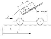
Figure 2: Mass-on-car system. The figure is based on [46, 15].

The second mass is coupled to the car by a spring-damper combination, and the ramp is inclined by a fixed angle $\vartheta\in(0,\pi/2)$. The equations of motion are given by

$$\begin{bmatrix}m_{1}+m_{2}&m_{2}\cos(\vartheta)\\ m_{2}\cos(\vartheta)&m_{2}\end{bmatrix}\!\!\begin{pmatrix}\ddot{z}(t)\\ \ddot{s}(t)\end{pmatrix}\!+\!\begin{pmatrix}0\\ ks(t)+d\dot{s}(t)\end{pmatrix}=\begin{pmatrix}u(t)\\ 0\end{pmatrix},$$ (7a)

where $$z s$$ is the car’s horizontal position, and  is the relative position of the second mass. As output the second mass’ horizontal position is measured

$$y(t)=z(t)+\cos(\vartheta)s(t).$$ (7b)

For simulation we choose the parameters $\vartheta=\pi/4$, $m_{1}=1$, $m_{2}=2$, spring constant $k=1$, and damping $d=1$. A short calculation yields that for these parameters system (7) has relative degree $r=2$, and as outlined in [15, Sec. 3] it can be represented in the form (1) with BIBO internal dynamics. We simulate output reference tracking of the signal $y_{\operatorname*{ref}}=0.4\sin(\tfrac{\pi}{2}t)$ for $t\in[0,1]$, transporting the mass $m_{2}$ on the car from position $0$ to $0.4$ within chosen error boundaries $\pm 0.15$. We choose the activation threshold ${\lambda=0.75}$. With these parameters a brief calculation yields $f_{\rm max}\leq 1.4$, $g_{\rm min}=g_{\rm max}=0.25$, and hence, the sampling time $\tau\leq 4.8\cdot 10^{-3}$, and the gain $\beta\geq 27.55$, which guarantee success of the tracking task. Choosing the smallest $\beta$ this already gives $\|u_{\rm ZoH}\|_{\infty}\leq\beta/\lambda\leq 36.73$. We start with a small initial tracking error $y(0)=-0.0925$, and $\dot{y}(0)=\dot{y}_{\rm ref}(0)$. We compare the controller (3) with the continuous funnel controller [15]; corresponding signals have the subscript $\rm FC$, e.g., $u_{\rm FC}$. Moreover, simulating the ZoH controller was even successful for $\tau=2.0\cdot 10^{-2}$ and $\beta=4$; corresponding signals have a circumflex, e.g., $\hat{y}_{\rm ZoH}$. Figure 3 shows the system’s output and the reference plus/minus error tolerance. Note that although the control input is discontinuous, the output signal is continuous due to integration.

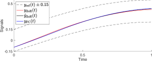
Figure 3: Outputs, reference, and error tolerance.

All controllers achieve the tracking task. In Figure 4 the controls are depicted.

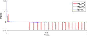
Figure 4: Controls.

The ZoH input consists of separated pulses - for two reasons. First, the control law (3) uses (undirected) worst-case estimations $g_{\rm min},g_{\rm max}$ and $f_{\rm max}$ to compute the input signal. Hence, the control signal is at many time instances unnecessary large; however, it is ensured that the control signal is sufficiently large for all times. Second, (3) involves an activation threshold $\lambda$, i.e., the controller is inactive, if the tracking error is small. If at sampling the tracking error is above this threshold, the applied input is sufficiently large (due to the worst case estimations) to push the error back below the threshold. Thus, at the next sampling instance the input is determined to be zero. The worst-case estimations and the ZoH setting make it inevitable that the control signal looks peaky. The control signal $\hat{u}_{\rm ZoH}$ (black) is also peaky, but not so large in magnitude (smaller $\beta$) and with a larger width (larger $\tau$). Overall, $\hat{u}_{\rm ZoH}$ is comparable with $u_{\rm FC}$. The success of the simulation with these parameters gives rise to the hope of finding better estimates for sufficient control parameters $\beta,\tau$ in future work. Improving the control performance is also topic of Section 5. Note that the control signal $u_{\rm FC}$ also has a large peak at the beginning, where $\|u_{\rm FC}\|_{\infty}\approx 100$. For simulation, we used Matlab, for integration of the dynamics the routine ode15s with $\rm AbsTol=RelTol=10^{-6}$, with adaptive step size. Integrating the funnel controller [15] ode15s yields that the maximal step size is $\approx 3.99\cdot 10^{-2}$ and the minimal step size is $\approx 1.21\cdot 10^{-6}$. This means, the largest step is about eight times larger than $\tau$, and the smallest time step is about 4000 times smaller than $\tau$.

5 Two-component data-driven controller

As can be seen from the numerical simulation in Section 4, the control signal $u_{\rm ZoH}$ exhibits undesirably large peaks. This is due to the worst case estimations in the controller design. In this section, a basic idea for improving the control signal is explained using two example techniques.

These ideas are based on the observation made in Remark 3.2, namely if $\|e_{r}(t_{k})\|<\lambda$, then any bounded input $u$ can be applied to the system. In particular, data-driven control schemes are applicable, which often show superior performance due to collection of “system knowledge” in terms of input-output data. The idea of a combined control scheme is illustrated in Figure 5.

Figure 5: Schematic structure of the combined controller.

Since the calculations in the proof of Theorem 3.1 involve worst case estimates, the application of $u(t)\neq 0$ for $t\in[t_{k},t_{k}+\tau)$, if $\|e_{r}(t_{k})\|<\lambda$ requires adaption of the sampling time $\tau$. This adaption is formulated in the following feasibility result for the switched control strategy

$$\!\!\forall t\in[t_{k},t_{k+1}):u(t)=\begin{cases}\quad u_{\rm data},\!\!&\|e_{r}(t_{k})\|<\lambda,\\ -\beta\tfrac{e_{r}(t_{k})}{\|e_{r}(t_{k})\|^{2}},\!\!&\|e_{r}(t_{k})\|\geq\lambda.\end{cases}$$ (8)

Theorem 5.1.

Given a reference $y_{\operatorname*{ref}}\in W^{r,\infty}(\mathds{R}_{\geq 0},\mathds{R}^{m})$ and a funnel function $\varphi\in\mathcal{G}$ consider a system (1) with $(d,f,g,\mathbf{T})\in\mathcal{N}^{m,r}$. Let the constants given in (4), and $\kappa_{0},\kappa_{1}$ and $\beta$ be given as in Theorem 3.1. Assume that the initial condition satisfies $\chi(y^{0})(0)\in\mathcal{D}_{0}^{r}$ and, for an activation threshold ${\lambda\in(0,1)}$, and $u_{\rm max}\geq 0$ let the sampling time satisfy

$$0<\tau\leq\min\left\{\frac{\kappa_{0}}{\kappa_{1}^{2}},\frac{1-\lambda}{\kappa_{0}+\|\varphi\|_{\infty}g_{\rm max}u_{\rm max}}\right\}.$$ (9)

If $\|u_{\rm data}\|_{\infty}\leq u_{\rm max}$, then the combined controller (8) applied to a system (1) yields that $\|e_{k}(t)\|<1$ for all $k=1,\ldots,r-1$ and $\|e_{r}(t)\|\leq 1$ for all $t\geq 0$. This is initial and recursive feasibility of the controller (8). In particular, the tracking error satisfies $\|e(t)\|<1/\varphi(t)$ for all $t\in\mathds{R}_{\geq 0}$.

Proof.

By adapting the sampling time $\tau$ the statement follows with the same proof as for Theorem 3.1. ∎

With Theorem 5.1 at hand, we may now consider the following extensions of the control law (3), resulting in a combined controller (8).

Remark 5.1.

We emphasise that none of the control schemes applied if $\|e_{r}(t_{k})\|<\lambda$ are required to achieve any tracking guarantees. The only requirement is that the control signal $u_{\rm data}$ satisfies $\|u_{\rm data}\|_{\infty}\leq u_{\rm max}$ for given $u_{\rm max}>0$. In particular, this means that any predictive controller applied in the safe region satisfies input constraints given by $u_{\rm max}$. Moreover, a control scheme applied in the safe region is not even supposed to be suitable for the system to be controlled. Since the sampling time is sufficiently small, the feedback law $-\beta e_{r}(t_{k})/\|e_{r}(t_{k})\|^{2}$ maintains the tracking guarantees in case of failure of $u_{\rm data}$.

Remark 5.2.

The input $u_{\rm data}$ in (8) is not necessarily supposed to be of data-driven or learning-based type. A sample-and-hold version of the funnel control law [15], i.e.,

$$u_{\rm data}(t)=-\alpha(\|e_{r}(t_{k})\|^{2})e_{r}(t_{k}),\quad t\in[t_{k},t_{k}+\tau)$$ (10)

is feasible with $u_{\rm max}=\lambda/(1-\lambda^{2})$. This choice approximates the continuous funnel control signal on a fixed time grid. Since this discrete-time funnel controller is safeguarded by the ZoH controller in (8), none of the issues regarding feasibility of this sampled-and-hold funnel control signal (cf. the considerations in [14]) are present. If a nominal model of the system is available, another combined controller strategy would be to include a pre-computed feedforward signal, cf. [47], with $u=u_{\rm feedforward}+u_{\rm ZoH}$ where the feedforward controller is active in the safe as well in the safety-critical region. The controller (8) would interpret this additional signal as a “helpful” disturbance (“helpful” since it will reduce the control effort of the feedback), and constraint satisfaction is guaranteed.

5.1 Data-driven MPC using Willems’ fundamental lemma

In this section we propose a control regime for the safe region established by a data-driven MPC scheme based on the fundamental lemma by Willems et al. [24]. We consider a surrogate model for the system (1) given by a discrete-time linear time-invariant system in minimal, i.e. controllable and observable, state-space realization

$$x_{k+1}=Ax_{k}+Bu_{k}$$ (11a)

$$y_{k}=Cx_{k}+Du_{k}$$ (11b)

with matrices $A\in R^{n\times n}$, $B\in\mathds{R}^{n\times m}$, $C\in\mathds{R}^{m\times n}$ and $D\in\mathds{R}^{m\times m}$. Except the dimension $m$, which is determined by the input and output dimension of the system (1), the parameters $A,B,C,D$ are assumed to be unknown.

Next we recall the property of persistency of excitation and the fundamental lemma for controllable systems by Willems et al. [24], which are pivotal elements in the subsequent discussion. A sequence $u=(u_{k})_{k=0}^{N-1}$ with $u_{k}\in\mathds{R}^{m}$, $k=0,\dots,N-1$, is called persistently exciting of order $L$, $L\in\mathds{N}$, if the Hankel matrix

$$H_{L}(u):=\begin{bmatrix}u_{0}&\dots&u_{N-L}\\ \vdots&\ddots&\vdots\\ u_{L-1}&\dots&u_{N-1}\end{bmatrix}\in\mathds{R}^{mL\times(N-L+1)}$$ (12)

has full row rank.

Lemma 5.1 (Fundamental lemma).

Let $(\hat{u},\hat{y})=((\hat{u}_{k})_{k=0}^{N-1},(\hat{y}_{k})_{k=0}^{N-1})$ be an input-output trajectory of length $N$, $N\in\mathds{N}$, of the system (11) such that $\hat{u}$ is persistently exciting of order $L+n$, where $L\in\mathds{N}$ and $n$ is the state dimension of system (11). Then $(u,y)=((u_{k})_{k=0}^{L-1},(y_{k})_{k=0}^{L-1})$ is an input-output trajectory of length $L$ of system (11) if and only if there is $\nu\in\mathds{R}^{N-L+1}$ such that

$$\begin{bmatrix}u_{[0,L-1]}\\ y_{[0,L-1]}\end{bmatrix}=\begin{bmatrix}H_{L}(\hat{u})\\ H_{L}(\hat{y})\end{bmatrix}\nu.$$ (13)

The fundamental lemma allows a complete non-parametric, data-driven description of the system’s finite-length input-output trajectories based only on measured input-output data.

Remark 5.3.

Note that persistency of excitation order $\tilde{L}$ implies persistency of excitation of lower order $L$, $L\leq\tilde{L}$. This fact might be exploited in situations where the state dimension $n$ of a suitable surrogate model (11) is unclear but can be estimated, for instance, from physical interpretations of the underlying system (1). At worst overestimation of $n$ results in an increased data demand for the signal $(\hat{u},\hat{y})$, while the representation (13) is maintained.

Next we introduce an data-driven MPC scheme leveraged by the fundamental lemma , Lemma 5.1. To this end let $(\hat{u},\hat{y})=((\hat{u}_{k})_{k=0}^{N-1},(\hat{y}_{k})_{k=0}^{N-1})$ be measured input-output data, where $\hat{u}$ is persistently exciting of order $L+2n$. In every discrete time step $t_{k}$ we aim to solve the optimal control problem

$$\operatorname*{minimize}_{(u,y,\nu,\sigma)}\sum_{i=k+1}^{k+L}\Bigl{(}\lVert y_{i}-y_{\text{ref},i}\rVert_{Q}^{2}+\lVert u_{i}\rVert_{R}^{2}\Bigr{)}+\lambda_{\nu}\lVert\nu\rVert^{2}+\lambda_{\sigma}\lVert\sigma\rVert^{2}$$ (14a)

with $$(u,y)=((u_{i})_{i=k-n+1}^{k+L},(y_{i})_{i=k-n+1}^{k+L})$$ subject to

$$\begin{bmatrix}u_{[k-n+1,k+L]}\\ y_{[k-n+1,k+L]}\end{bmatrix} =\begin{bmatrix}H_{L+n}(\hat{u})\\ H_{L+n}(\hat{y})\end{bmatrix}\nu,$$ (14b)

$$\begin{bmatrix}u_{[k-n+1,k]}\\ y_{[k-n+1,k]}\end{bmatrix} =\begin{bmatrix}\tilde{u}_{[k-n+1,k]}\\ \tilde{y}_{[k-n+1,k]}\end{bmatrix}+\sigma,$$ (14c)

$$\lVert u_{i}\rVert \leq u_{\text{max}},\ i=k+1,\dots,k+L$$ (14d)

on a finite horizon $L>0$, given a past input-output trajectory $(\tilde{u},\tilde{y})=((\tilde{u}_{i})_{i=k-n}^{k},(\tilde{y}_{i})_{i=k-n}^{k})$, where $\tilde{u}_{i}=u(t_{i})$, $\tilde{y}_{i}=y(t_{i})$ with $u$, $y$ denote the input and output of system (1), respectively. The weighting matrices $Q,R\in\mathds{R}^{m\times m}$ in the stage cost in (14a) are assumed to be symmetric and positive-definite. As a key difference to standard MPC the state-space model (11) is replaced in the optimal control problem (14) by the equivalent non-parametric description (14b) based on Lemma 5.1. The constraint (14c) serves as initial condition which together with the observability of surrogate model (11) imposes alignment on the latent state, i.e. $x_{[k-n+1,k]}=\tilde{x}_{[k-n+1,k]}$ for the state sequences $(x_{i})_{i=k-n+1}^{k}$ and $(\tilde{x}_{i})_{i=k-n-1}^{k}$ corresponding to the input-output trajectories $((u_{i})_{i=k-n+1}^{k},(y_{i})_{i=k-n+1}^{k})$ and $((\tilde{u}_{i})_{i=k-n+1}^{k},(y_{i})_{i=k-n+1}^{k})$. In order to take into account model mismatches due to nonlinearity of the underlying system (1) we introduce a slack variable $\sigma\in\mathds{R}^{2nm}$ and the cost functional in (14a) involves a regularization in terms of $\nu$ with weighting parameters $\lambda_{\nu}>0$, $\lambda_{\sigma}>0$. Further, we impose input constraints in (14d). The data-driven MPC scheme is summarized in Algorithm 1.

In practice the observed past trajectory $(\tilde{u},\tilde{y})$ sampled from the system (1) up to a certain point in time may serve as source for the data $(\hat{u},\hat{y})$ deployed in the system description (14c) via Hankel matrices. With this choice more and more data is available with increasing time and, hence, in this way a higher persistency of excitation order can be achieved. As an extension to the above proposed data-driven MPC strategy one may allow for a prediction horizon $L$, which increases over time whenever the updated data is persistently exciting of sufficient order.

Algorithm 1 Data-driven MPC with error guarantees

$PE\leftarrow\text{false}$; $k=0,1,\dots$

get latest sample point $(\tilde{u}_{k},\tilde{y}_{k})$;

calculate $\|e_{r}(t_{k})\|$; not $PE$$\triangleright$ learn the dynamics

update data $(\hat{u},\hat{y})$, $\hat{u}_{k}\leftarrow\tilde{u}_{k}$, $\hat{y}_{k}\leftarrow\tilde{y}_{k}$; $\hat{u}$ is p.e. of order $L+n$

$PE\leftarrow\text{true}$;

store $\mathcal{H}_{L+n}(\hat{u})$, $\mathcal{H}_{L+n}(\hat{y})$; $\left\|e_{r}(t_{k})\right\|<\lambda$ PE $\triangleright$ MPC feedback

$u_{\text{act}}\leftarrow$ solve(OCP (14)); $\triangleright$ random input action

$u_{\text{act}}\leftarrow\text{random (bounded by $u_{\max}$)}$; $\triangleright$ sampled-data feedback

$u_{\text{act}}\leftarrow-\beta\frac{e_{r}(t_{k})}{\left\|e_{r}(t_{k})\right\|^{2}}$;

apply $u_{\text{act}}$ as ZoH input action to the system (1)

The ZoH feedback law (3) involves the recursively defined auxiliary error variables $e_{j}$ defined in (2), which in particular involve higher-order derivatives of both the system output $y$ and the reference signal $y_{\rm ref}$. To take the structure of these $e_{j}$ into account in the data-driven MPC scheme, we aim to include information on these derivatives in the cost function. However, since the data-driven framework is formulated for discrete-time models (11), we use finite differences to approximate the output’s derivatives, i.e., we use $\frac{y_{i}-y_{i-1}}{\tau}=:y^{[1]}_{i}$. Higher-order derivatives are approximated accordingly, and we denote with $y^{[\ell]}_{i}=\tfrac{1}{\tau^{\ell}}\sum_{j=0}^{\ell}(-1)^{j}\binom{j}{\ell}y_{i-j}$ for $y_{i}$ being the output of (11) the backwards finite difference approximation of the $\ell^{\rm th}$-order derivative. Furthermore, we want to take into account the weighting of the higher-order derivatives. To see, how the derivatives are to be weighted, we explicate the error variable $e_{3}$ (we omit the time argument) using the bijection $\alpha(s)=1/(1-s)$, and obtain

$$e_{3} =\varphi\ddot{e}+\frac{1}{1-\|e_{2}\|^{2}}e_{2}$$ (15)

$$=\varphi\ddot{e}+\frac{1}{1-\|e_{2}\|^{2}}\Big{(}\varphi\dot{e}+\frac{1}{1-\|e_{1}\|^{2}}e_{1}\Big{)}$$

$$=\varphi\Big{(}\ddot{e}+\underbrace{\frac{1}{1-\|e_{2}\|^{2}}}_{\geq 1}\dot{e}+\underbrace{\frac{1}{1-\|e_{2}\|^{2}}}_{\geq 1}\underbrace{\frac{1}{1-\|e_{1}\|^{2}}}_{\geq 1}e\Big{)}.$$

From this it is clear that the weighting is decreasing with increasing order of the derivative. Combining the regularisation in (14) and the previous reasoning, we propose the following cost functional

$$\begin{split}\sum_{i=k+1}^{k+L}&\Bigl{(}\sum_{\ell=0}^{r-1}\varphi(t_{i})\mu_{\ell}\|y_{i}^{[\ell]}-y_{\rm ref}^{(\ell)}(t_{i})\|^{2}_{Q}+\|u_{i}\|^{2}_{R}\Bigr{)}\\ &{}+\lambda_{\nu}\lVert\nu\rVert^{2}+\lambda_{\sigma}\lVert\sigma\rVert^{2},\end{split}$$ (16)

where $\mu_{0}\geq\mu_{1}\geq\cdots\geq\mu_{r-1}\geq 0$, and $\varphi(t_{i})$ is the funnel function evaluated at $t=t_{i}$. The weights $\mu_{\ell}$ reflect the weighting structure in the auxiliary error variables, see (15). Note that $1/(1-s^{2})=1$ if and only if $s=0$, i.e., it is reasonable to order the factors $\mu_{\ell}$ strictly.

In the following we demonstrate the data-enabled MPC scheme described in Algorithm 1 on the example system (7) with fixed prediction horizon $L=20$. Because of the linearity of system (7) we waive the slack variable in the optimal control problem (14), i.e. we set $\sigma=0$. We set $u_{\text{max}}=10$ which yields $\tau\leq 2.8\cdot 10^{-3}$ according to (9). As weights we choose $Q=10^{3}\cdot I$, $R=10^{-4}\cdot I$, $\lambda_{\nu}=10^{-6}$. We consider a constant funnel given by $\varphi(t)=0.15$. The output tracking, the control signal and the auxiliary error variables are depicted in Figure 6, Figure 7 and Figure 8 in blue, respectively. In the beginning, there is random control in order to generate a persistently exciting input signal. Then, at $t=0.2728$ persistency of excitation is reached and MPC produces a control signal, however, the error $e_{2}$ exceeds the safety region. Hence, the ZoH signal becomes active. In the subsequent phase the system is governed by the MPC component, while the signal is saturated at $-u_{\text{max}}$. Again the error variable $e_{2}$ leaves the the safety region at $t=0.3770$ and the ZoH component takes over, resulting in a large control input, which is applied for one sampling interval. Afterwards, MPC again is sufficient to keep $e_{2}$ and $e_{1}$ below $\lambda$ and maintains the tracking goal.

In a second numerical experiment we extend the MPC strategy towards higher auxiliary error variables in the cost functional and an adaptively increasing prediction horizon. The performance is depicted in  Figure 6, Figure 7 and Figure 8 in red. Starting with $L=1$ the prediction horizon is allowed to increases over time until $L=20$. Further, we set $Q=10^{3}\cdot I$, $R=10^{-4}\cdot I$, $\lambda_{\nu}=10^{-6}$ as before, and $\mu_{0}=\frac{1}{\varphi(0)}$, $\mu_{1}=\frac{1}{\varphi(0)}\cdot 10^{-2}$, where the funnel is constant with $\varphi(t)=0.15$. In comparison to the first experiment one observes that the enhanced MPC strategy suffices to safeguard both error variables and, therefore, at no time the ZoH component becomes active. The tracking performance in both runs is of similar quality.

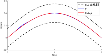
Figure 6: Outputs, reference, and boundaries.

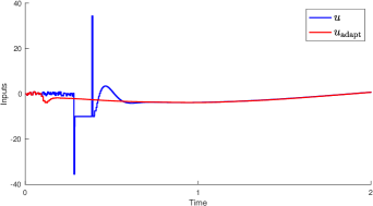
Figure 7: Controls.

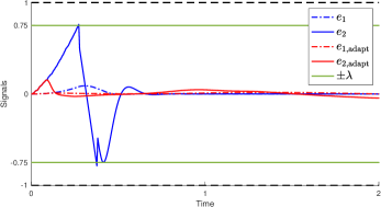
Figure 8: Error variables.

5.2 Reinforcement Learning: $Q$-table control

Using the example of $Q$-learning, we show, in this section, how the controller (3) can be combined with model-free reinforcement learning (RL) techniques to improve the control signal using the control strategy (8). $Q$-learning was first developed in [48] and has since become a cornerstone of reinforcement learning and foundation for many other learning algorithms [49].

To explain the basic concepts of $Q$-learning, we consider a nonlinear discrete-time control system of the form

$$x_{k+1}=f\big{(}x_{k},u_{k}\big{)}$$ (17)

where $x\in\mathcal{X}\subset\mathds{R}^{n}$ is the state of the system, $u\in\mathcal{U}\subset\mathds{R}^{m}$ is the control input, and $f:\mathcal{X}\times\mathcal{U}\to\mathcal{X}$ is an unknown function. Given an initial state $x^{0}\in\mathcal{X}$, we denote for a control sequence $u=(u_{k})\in\mathcal{U}^{\mathds{N}}$, the solution of (17) by $x(\cdot;x^{0},u)$. We further assume that there exists a bounded function $r:\mathcal{X}\times\mathcal{U}\to\mathds{R}$, which is also called reward function. Note that we do not assume the function $r$ to be known but that merely at every step $k\in\mathds{N}$ of the system (17) the reward $r(x_{k},u_{k})$ can be obtained. The objective is to maximise the cumulative future reward, i.e. to solve the optimisation problem

$$\mathop{\operatorname{maximize}}_{u\in\mathcal{U}^{\mathds{N}}}\ \sum_{k=0}^{\infty}\gamma^{k}r(x(k;x^{0},u),u_{k})$$ (18)

with discount factor $\gamma\in(0,1)$ which determines the relative importance of long-term versus short-term future rewards. The so called $Q$-function $Q:\mathcal{X}\times\mathcal{U}\to\mathds{R}$ defined by

$$Q(\hat{x},\hat{u}):=r\big{(}\hat{x},\hat{u}\big{)}+\gamma\sup_{u\in\mathcal{U}^{\mathds{N}}}\sum_{k=0}^{\infty}\gamma^{k}r(x(k;f(\hat{x},\hat{u}),u),u_{k}).$$ (19)

plays a key role for solving the optimisation problem.

Theorem 5.2 ([42, Sec. 1.1]).

Consider the system (17). If $\pi:\mathcal{X}\to\mathcal{U}$ is a feedback control with

$$\pi(x)\in\mathop{\operatorname{argmax}}_{u\in\mathcal{U}}Q(x,u)$$ (20)

for all $x\in\mathcal{X}$, then $\pi$ applied to the system (17) is a solution to the optimisation problem (18).

If the Q-function is known, then an optimal feedback control $\pi$, in the sense of solving the optimisation problem (18), can be calculated. Its simplicity makes the optimal feedback control, also known as optimal policy, very appealing. This however gives rise to the problem of approximating or learning the $Q$-function (19). While there exist various modern approaches addressing the problem [49], the original $Q$-learning algorithm from [48] takes the form Algorithm 2.

Algorithm 2 Q-learning algorithm

1. Initialise $j=0$, $\tilde{Q}_{0}(x,u):=0$, let state $x\in\mathcal{X}$, select a learning rate $(\alpha_{k})\in[0,1)^{\mathds{N}}$.

2. Select $u\in\mathcal{U}$, observe $x^{\prime}=f(x,u)\in\mathcal{X}$.

3. Update

   $$\tilde{Q}_{k+1}(x,u)\!:=\!(1-\alpha_{k})\tilde{Q}_{k}(x,u)+\alpha_{k}\!\!\left(\!\!r(x,u)\!+\!\gamma\max_{u^{\prime}\in\mathcal{U}}\tilde{Q}_{j}(x^{\prime},u^{\prime})\!\!\right)\!\!.$$

4. Set $x:=x^{\prime}$, increase $j$ by one, and go to (2).

An essential part of Algorithm 2 is the selection of the control action in Step 2. One has to find a balance between selecting the currently expected optimal control and selecting a different action hoping it yields a higher cumulative reward in the future. There exist several strategies to address this exploration-exploitation dilemma, see e.g. [50]. One of the commonly used selection of the control action in the Step 2 of Algorithm 2 is an $\varepsilon$-greedy choice. For a given $\varepsilon\in[0,1]$, the control action is selected as $u=\max_{u\in\mathcal{U}}\tilde{Q}_{j}(x,u)$ with the probability of $1-\varepsilon$ and an arbitrary control $u\in\mathcal{U}$ is selected with probability of $\varepsilon$.

The learning rate $(\alpha_{k})$ plays also a crucial role in addressing the exploration-exploitation dilemma. It determines the extent to which Algorithm 2 updates its estimate of the $Q$-function during each iteration by new information. It is a decisive factor in the convergence rate of the learning algorithm, see e.g. [51].

Theorem 5.3 ([52]).

Consider the system (17) with finite sets $\mathcal{X}$, $\mathcal{U}$. If the learning rate $(\alpha_{k})\in\ell^{2}(\mathds{N})\backslash\ell^{1}(\mathds{N})$ and if all $(x,u)\in\mathcal{X}\times\mathcal{U}$ appear infinitely often in Step $2$ of the algorithm, then

$$\lim_{k\to\infty}\tilde{Q}_{k}(x,u)=Q(x,u)$$

for all $x\in\mathcal{X}$, $u\in\mathcal{U}$.

In view of Theorem 5.3, combining $Q$-learning with the controller (3) in the form of a combined controller (8) and applying it to the system (1) faces three challenges which need to be addressed: $Q$-learning is formulated for discrete systems, the sets $\mathcal{X}$, $\mathcal{U}$ are assumed to be finite, and the problem is presumed to be time-invariant. Under the assumption that the operator $\mathbf{T}$ does not have a time-delay, using a sampling rate $\tau>0$ and only applying constant control signals between two sampling times puts the system (1) via evaluation of its solution operator into a discrete system of the form (17). There are various approaches to overcome the requirement of a finite state and control space $\mathcal{X}$, $\mathcal{U}$, see e.g. [53]. As a consequence of Lemma 2.1, the states $\chi(y)$, respectively the error signals $e_{i}$ for $i=1,\ldots,r-1$, of the system (1), evolve within a compact set $K$ when applying the combined controller (8) to the system (1). Using a discretization of this compact set is, therefore a straightforward way to overcome the problem of the requirement of a finite set $\mathcal{X}$. Since the controller (3) is bounded by $\beta/\lambda$, a discretization of the set $\bar{\mathcal{B}}_{\beta/\lambda}$ is a natural choice for $\mathcal{U}$. However, the curse of dimensionality renders a discretization approach unsuitable for high-dimensional problems. Due to the dependence of $y_{\operatorname*{ref}}$ and $\varphi$ on $t$, the considered problem is inherently time variant. There are a number of different results for addressing this issue, see e.g. [54, 55]. It is also possible to encode this time dependency in the state of the system (17) by enlarging the compact set $K$ and modifying (17), because the functions $y_{\operatorname*{ref}}$ and $\varphi$ are bounded. However, one cannot guarantee that all $(x,u)\in\mathcal{X}\times\mathcal{U}$ appear infinitely often in the algorithm, unless $y_{\operatorname*{ref}}$ and $\varphi$ are periodic. Furthermore, encoding the time dependency in the compact set $K$ further worsens the problem of the curse of dimensionality. Nevertheless, in virtue of Remark 5.1 it is still meaningful to combine the Q-learning scheme with the ZoH controller (3).

In the following we demonstrate the combined controller (8) consisting of (3) and the $Q$-learning Algorithm 2 on the example system (7). Using the control strategy (8) with sampling time $\tau>0$ and time instances $t_{k}\in\tau\mathds{N}$, the aim is to take advantage of $Q$-learning by exploring the safe tracking region, e.g. for $\left\|e_{r}(t_{k})\right\|<\lambda$, and applying an improved control signal while the safety critical region is secured by the controller $u_{\rm ZoH}$ as in (3) for $\|e_{r}(t_{k})\|\geq\lambda$. We, therefore, only consider the error variable $e_{r}$ for the $Q$-learning Algorithm 2 and choose a uniform discretization of the set $\bar{\mathcal{B}}_{\lambda}$ as the state space $\mathcal{X}$. Considering the system (1) and the error variables (2), $e_{r}$ satisfies the ordinary differential equation

$$\dot{e}_{r}(t) =\frac{\dot{\varphi}(t)}{\varphi(t)}(e_{r}(t)-\gamma_{r-1}(t))+\dot{\gamma}_{r-1}(t)$$

$$\phantom{=}+\varphi(t)(f({z}(t))+g({z}(t))u-y_{\operatorname*{ref}}^{(r)}(t)),$$

with $\gamma_{r-1}(t):=\alpha(\|e_{r-1}(t)\|^{2})e_{r-1}(t)$ and ${z}(\cdot):=(d(\cdot),\mathbf{T}(\chi(y))(\cdot))$. Sampling this differential equation with sampling time $\tau$ results in a discrete-time control system. However, note that it does not have the form (17) due to the time dependency of $y_{\operatorname*{ref}}$ and $\varphi$, and the state variables $e_{1},\ldots,e_{r-1}$ are neglected. Nevertheless, the application of the $Q$-learning algorithm achieves that the error variable $e_{r}$ remains, after an initial learning period, below the threshold $\lambda$ as simulations show, see Figures 9 and 10. Further research is necessary to determine whether it is always the case that solely considering $e_{r}$ in the $Q$-learning algorithm is sufficient and if guarantees about the convergence of the learning algorithm can be given despite the inherent time dependency of the problem. As for the set of control values, we choose $\mathcal{U}$ to be a uniform discretization of the set $\bar{\mathcal{B}}_{u_{\max}}$ where $u_{\max}$ is chosen as $u_{\max}=10$ as in the example in Section 5.1. To improve the performance of the original controller (3), meaning better tracking performance and reduced control values, we choose the reward function

$$r(e_{r}(t_{k}),u)=-\left\|e_{r}(t_{k})\right\|^{2}-\alpha_{u}\left\|u\right\|^{2},$$

with parameter $\alpha_{u}\in\mathds{R}_{\geq 0}$. The function $r$ rewards small values of the error variable $e_{r}$ and the applied control values (depending on the penalty parameter $\alpha_{u}$). For the simulation of the example system (7) we chose the system parameters as in Section 4. The reference trajectory was selected as $y_{\operatorname*{ref}}=0.4\sin(\tfrac{\pi}{4}t)$ for $t\in[0,20]$. Further for the $Q$-learning parameters, the dimensions of the finite sets $\mathcal{X}$ and $\mathcal{U}$ were selected as $8$ and $25$, respectively. The learning rate is set as constant $\alpha=0.8$. In order to let the algorithm explore more, the greedy parameter is set to $\varepsilon=1$ for $t\in[0,1]$, then a decay parameter with a value of $\varepsilon_{d}=0.5$ was applied every second in order to take the control action more often according to learned $Q$-function. For the reward function the parameter $\alpha_{u}=1/u_{\text{max}}$ was selected. The simulations are depicted in Figures 9 and 10. Figure 9 shows how the error signals evolve within the funnel, respectively the $\lambda$ activation threshold. Figure 10 shows the corresponding control action. It can be seen that with the help of the primary controller $u_{\rm ZoH}$ in (3), Q-learning algorithm is able to explore and learn safely. The learning controller component applies random control actions with an amplitude lower than $10$ to explore the state and control space. Only if the error is larger than the activation threshold, the ZoH control component intervenes with a large control input to prevent a violation of the funnel boundaries. One can see that with decaying $\varepsilon$ the number of random control actions applied to the system reduces and the error $e_{2}(t)$ signal gets closer to $0$ and remains close to it. Overall, the $Q$-learning algorithm reduces the peaks of the control significantly in comparison to Section 4 where merely the controller (3) was applied.

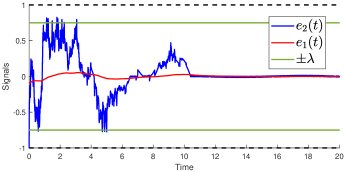
Figure 9: Error signals.

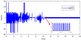
Figure 10: Control signals.

Remark 5.4.

To reduce computational effort, the control signal $u_{\rm data}$ in (8) does not have to be updated at every $t_{i}=i\tau$. Since the system class (1) allows for bounded disturbances, it is possible to combine the data-driven control with a move blocking strategy, cf. [56], i.e., to apply the control value $u_{\rm data}$ for longer than one sampling interval $\tau$. If then $e_{r}$ leaves the safe region, the controller (8) interprets the additional value $u_{\rm data}$ as a disturbance in the system (according to Assumption 1 this means $D=\|d\|_{\infty}+u_{\rm max}$), and hence the constraint satisfaction is guaranteed by the controller. Note that system measurements, however, have to be taken at every $t_{i}=i\tau$.

6 Conclusion and future work

We presented a novel two-component controller for continuous-time nonlinear control systems. The ZoH tracking controller consists of a data-driven/learning-based component and a discrete-time output-feedback controller with prescribed performance. The feedback controller is designed to achieve the control objective (tracking with prescribed performance) and safeguards the learning-based controller. We derived explicit upper bounds on the sampling time $\tau>0$ and for the maximal control input. As data-driven controller we employed an MPC algorithm based on the fundamental results of Willems et al. [24], which enables predictive control using only input-output data. Further, we implemented a reinforcement learning scheme and investigated a Q-table control algorithm to explore the system’s dynamics. The proposed two-component data-driven controller was proven to achieve the control objective, and in particular, outperform the pure feedback controller.

Based on the presented results, future work will aim to reduce the conservatism of the controller and to investigate the interplay with observers and/or the funnel pre-compensator [57, 58] to alleviate the strict assumption of not only knowing the output but also its derivatives. Moreover, we plan to perform a comprehensive comparison (simulation study) with other data-driven ZoH controllers, e.g., the one recently proposed in [59], and combining these with the proposed safeguarding feedback component.

Appendix A Proofs of auxiliary results

We present the proofs of the auxiliary results Lemmata 2.1 and 2.2 presented in Section 2.2, and Theorem 3.1 in Section 3.

Proof of Lemma 2.1.

We use the constants $\varepsilon_{k},\mu_{k}>0$ defined in (4), and to improve legibility, we use the notation $e_{k}(t):=e_{k}(t,\chi(\zeta)(t))$ for $\zeta\in\mathcal{Y}_{\delta}^{r}$. Let $\delta\in(0,\infty]$ and $\zeta\in\mathcal{Y}^{r}_{\delta}$ be arbitrary but fixed. We define the auxiliary function $\gamma_{k}(t):=\alpha(\|e_{k}(t)\|^{2})e_{k}(t)$, and set $\gamma_{0}(\cdot)=\dot{\gamma}_{0}(\cdot)=0$. Note that for $k=1,\ldots,r-1$ each of the error signals defined in (2) satisfies for $t\in[0,\delta)$ the differential equation

$$\dot{e}_{k}=\frac{\dot{\varphi}}{\varphi}(e_{k}\!-\!\gamma_{k-1})\!+\!e_{k+1}\!\!+\!\dot{\gamma}_{k-1}-\!\alpha(\|e_{k}\|^{2})e_{k},$$

where the dependency on $t$ has been omitted and $e^{(k)}$ denotes the $k$-th derivative of $e(t)=\zeta(t)-y_{\operatorname*{ref}}(t)$. We observe

$$\dot{\gamma}_{k} =2\alpha^{\prime}(\|e_{k}\|^{2})\left\langle e_{k},\dot{e}_{k}\right\rangle e_{k}+\alpha(\|e_{k}\|^{2})\dot{e}_{k}.$$

Seeking a contradiction, we assume that for at least one ${\ell\in\{1,\ldots,r-1\}}$ there exists $t^{*}\in(0,\delta)$ such that $\|e_{\ell}(t^{*})\|^{2}>\varepsilon_{\ell}$. W.l.o.g. we assume that this is the smallest possible $\ell$. Invoking $\chi(y^{0})\in\mathcal{D}_{0}^{r}$ and continuity of the involved functions we may define $t_{*}:=\max\left\{\ t\in[0,t^{*})\ \left|\ \vphantom{t\in[0,t^{*})}\|e_{\ell}(t)\|^{2}=\varepsilon_{\ell}\ \right.\right\}$. Then, for $t\in[t_{*},t^{*}]$ we calculate, omitting again the dependency on $t$,

$$\tfrac{\text{d}}{\text{d}t}\tfrac{1}{2}\|e_{\ell}\|^{2}=\!\left\langle e_{\ell},\tfrac{\dot{\varphi}}{\varphi}(e_{\ell}-\gamma_{\ell-1})+e_{\ell+1}+\dot{\gamma}_{\ell-1}-\alpha(\|e_{\ell}\|^{2})e_{\ell}\right\rangle$$

$$\leq\!\|e_{\ell}\|\!\left(\left\|\frac{\dot{\varphi}}{\varphi}\right\|_{\infty}\!\!\!\!(1\!+\!\alpha(\varepsilon_{\ell-1}^{2})\varepsilon_{\ell-1})\!+\!1\!+\!\bar{\gamma}_{\ell-1}\!-\!\alpha(\varepsilon_{\ell}^{2})\varepsilon_{\ell}\!\right)\leq\!0,$$

in the last line we used the monotonicity of $\alpha(\cdot)$, the definition of $\varepsilon_{\ell}$, and that $\dot{\gamma}_{\ell-1}$ is bounded by minimality of $\ell$. Hence, the contradiction $\varepsilon_{\ell}<\|e_{\ell}(t^{*})\|^{2}\leq\|e_{\ell}(t_{*})\|^{2}=\varepsilon_{\ell}$ arises after integration. This yields boundedness of $e_{\ell},\gamma_{\ell}$. Using the derived bounds we estimate

$$\|\dot{e}_{\ell}\|\leq\left\|\frac{\dot{\varphi}}{\varphi}\right\|_{\infty}\!\!\!\!(1+\alpha(\varepsilon_{\ell-1}^{2})\varepsilon_{\ell-1})+1+\alpha(\varepsilon_{\ell}^{2})\varepsilon_{\ell}+\bar{\gamma}_{\ell-1}=\mu_{\ell}.$$

We conclude $\|e_{k}(t)\|\leq\varepsilon_{k}<1$ and $\|\dot{e}_{k}(t)\|\leq\mu_{k}$ for all $k=1,\ldots,r-2$ and all $t\in[0,\delta)$. For $k=r-1$ the same arguments are valid invoking $e_{r}:[0,\delta)\to\overline{\mathcal{B}_{1}}$. ∎

Proof of Lemma 2.2.

To prove the assertion, we invoke continuity of the system functions $f,g$ and the resulting boundedness on compact sets. According to Lemma 2.1, there exist ${\varepsilon_{k}\in(0,1)}$ for $k=1,\ldots,r-1$ such that

$$\!\ \forall\,\!\zeta\!\in\!\mathcal{Y}_{\infty}^{r}\ \forall\,t\in\mathds{R}_{\geq 0}\!\ \forall\,k=1,\ldots,r-1:\left\|e_{k}(t,{\chi}(\zeta)(t))\right\|\!{\leq}\varepsilon_{k}.$$

Further, $\|e_{r}(t,\chi(\zeta)(t))\|\leq 1$. Thus, due to the definition of $e_{k}$ in (2), there exists a compact set $K_{\zeta}\subset\mathds{R}^{rm}$ with

$$\ \forall\,\zeta\in\mathcal{Y}_{\infty}^{r}\ \forall\,t\in\mathds{R}_{\geq 0}:\quad\chi(\zeta)(t)\in K_{\zeta}.$$

Due to the BIBO property of the operator $\mathbf{T}$, there exists a compact set $K_{q}\subset\mathds{R}^{q}$ with $\mathbf{T}(\xi)(\mathds{R}_{\geq 0})\subset K_{q}$ for all ${\xi\in\mathcal{C}(\mathds{R}_{\geq 0},\mathds{R}^{rm})}$ with $\xi(\mathds{R}_{\geq 0})\subset K_{\zeta}$. For arbitrary ${\delta\in(0,\infty)}$ and $\zeta\in\mathcal{Y}_{\delta}^{r}$, we have, according to Lemma 2.1,

$$\ \forall\,t\in[0,\delta)\ \forall\,k=1,\ldots,r-1:\quad\left\|e_{k}(t,{\chi}(\zeta)(t))\right\|{\leq}\varepsilon_{k}.$$

Further, $\|e_{r}(t,\chi(\zeta)(t))\|\leq 1$. Thus, $\chi(\zeta)(t)\in K_{\zeta}$ for all ${t\in[0,\delta)}$. For every element $\zeta\in\mathcal{Y}_{\delta}^{r}$ the function $\chi(\zeta)|_{[0,\delta)}$ can smoothly be extended to a function $\tilde{\zeta}\in(\mathcal{C}(\mathds{R}_{\geq 0},\mathds{R}^{m}))^{r}$ with $\tilde{\zeta}(t)\in K_{\zeta}$ for all $t\in\mathds{R}_{\geq 0}$. Due to the BIBO property of the operator $\mathbf{T}$, we have $\mathbf{T}(\tilde{\zeta})(t)\in K_{q}$ for all $t\in\mathds{R}_{\geq 0}$. Since $\mathbf{T}$ is causal, this implies $\mathbf{T}(\chi(\zeta))|_{[0,\delta)}(t)\in K_{q}$ for all $t\in[0,\delta)$ and $\zeta\in\mathcal{Y}_{\delta}^{r}$. Define the compact set $K:=\overline{\mathcal{B}_{D}}\times K_{q}\subset\mathds{R}^{p+q}$. Since $f(\cdot)$ and $g(\cdot)$ are continuous, the constants $f_{\rm max}:=\max_{x\in K}f(x)$ and $g_{\rm max}:=\max_{x\in K}g(x)$ exist. For every $\delta\in(0,\infty]$, $\zeta\in\mathcal{Y}_{\delta}^{r}$, and $d\in L^{\infty}(\mathds{R}_{\geq 0},\mathds{R}^{p})$ with $\left\|d\right\|_{\infty}\leq D$ we have $\ \forall\,t\in[0,\delta):\quad(d(t),\mathbf{T}(\chi(\zeta))(t))\in K$. Therefore, we obtain $f_{\rm max}\geq\left\|f((d,\mathbf{T}(\chi(\zeta)))|_{[0,\delta)})\right\|_{\infty}$ and ${g_{\rm max}\geq\left\|g((d,\mathbf{T}(\chi(\zeta)))|_{[0,\delta)})\right\|_{\infty}}$. Since $g(x)$ is positive definite, for every $x\in K$ there exists $g_{\rm min}>0$ such that $g_{\rm min}\leq\frac{\left\langle z,g((d,\mathbf{T}(\chi(\zeta)))|_{[0,\delta)}(t))z\right\rangle}{\left\|z\right\|^{2}}$ for all $z\in\mathds{R}^{m}\backslash\left\{0\right\}$. ∎

Proof of Theorem 3.1.

The proof consists of two main steps. In the first step we establish the existence of a solution of the initial value problem (1), (3). In the second step we show feasibility of the proposed control law, i.e., all error variables are bounded by $\varepsilon_{k}$ and the tracking error evolves within the funnel boundaries.

Step 1. The application of the control signal (3) to system (1) leads to an initial value problem. If this problem is considered on the interval $[0,\tau]$, then there exists a unique maximal solution on $[0,\omega)$ with $\omega\in(0,\tau]$. If all error variables $e_{k}$ evolve within the set $\mathcal{B}_{1}$ for all $t\in[0,\omega)$, then $\|\chi(y)(\cdot)\|$ is bounded on the interval $[0,\omega)$ and, as a consequence of the BIBO condition of the operator, $\mathbf{T}(\cdot)$ is bounded as well. Then $\omega=\tau$, cf. [60, § 10, Thm. XX] and there is nothing else to show. Seeking a contradiction, we assume the existence of $t\in[0,\omega)$ such that $\|e_{k}(t)\|\geq 1$ for at least one $k=1,\ldots,r$. Invoking Lemma 2.1 it remains only to show that the last error variable $e_{r}$ satisfies $\|e_{r}(t)\|\leq 1$ for all $t\in[0,\omega)$. Before we do so, we record the following observation. For $\gamma_{r-1}(t):=\alpha(\|e_{r-1}(t)\|^{2})e_{r-1}(t)$ we calculate for ${z}(\cdot):=(d(\cdot),\mathbf{T}(\chi(y))(\cdot))$

$$\dot{e}_{r}(t)-\varphi(t)g({z}(t))u=\dot{\varphi}(t)e^{(r-1)}(t)+\varphi(t)e^{(r)}(t)$$ (21)

$$\quad+\dot{\gamma}_{r-1}(t)-\varphi(t)g({z}(t))u$$

$$=\frac{\dot{\varphi}(t)}{\varphi(t)}(e_{r}(t)-\gamma_{r-1}(t))+\dot{\gamma}_{r-1}(t)$$

$$\quad+\varphi(t)(f({z}(t))-y_{\operatorname*{ref}}^{(r)}(t))=:J(t).$$

Step 2. We show $\|e_{r}(t)\|\leq 1$ for all $t\in[0,\omega)$. We separately investigate the two cases $\|e_{r}(0)\|<\lambda$ and $\|e_{r}(0)\|\geq\lambda$.
Step 2.a We consider $\|e_{r}(0)\|<\lambda$. In this case we have $u=0$. Seeking a contradiction, we suppose that there exists $t^{*}:=\inf\left\{\ t\in(0,\omega)\ \left|\ \vphantom{t\in(0,\omega)}\|e_{r}(t)\|>1\ \right.\right\}$. For the function $J(\cdot)$ introduced in (21) we observe $\|J|_{[0,t^{*})}\|_{\infty}\leq\kappa_{0}$ according to Lemmata 2.1 and 2.2. Then we calculate for $t\in[0,t^{*}]$

$$1 =\|e_{r}(t^{*})\|\leq\|e_{r}(0)\|+\textstyle\int_{0}^{t^{*}}\!\!\|\dot{e}_{r}(s)\|\!\ \text{d}s$$

$$=\|e_{r}(0)\|+\textstyle\int_{0}^{t^{*}}\|J(s)\|\ \text{d}s$$

$$\leq\|e_{r}(0)\|+\textstyle\int_{0}^{t^{*}}\kappa_{0}\ \text{d}s<\lambda+\kappa_{0}\omega<1,$$

where we used $t^{*}<\omega\leq\tau<(1-\lambda)/\kappa_{0}$. This contradicts the definition of $t^{*}$.
Step 2.b We consider $\|e_{r}(0)\|\geq\lambda$. In this case we have the control $u=-\beta e_{r}(0)/\|e_{r}(0)\|^{2}$. We show again $\|e_{r}(t)\|\leq 1$ for all $t\in[0,\omega)$. To this end, seeking a contradiction, we suppose the existence of $t^{*}=\inf\left\{\ (0,\omega)\ \left|\ \vphantom{(0,\omega)}\|e_{r}(t)\|>1\ \right.\right\}$. Invoking the initial conditions and continuity of the involved functions, and utilising Lemma 2.2 and (21), we calculate for $t\in[0,t^{*}]$

$$\tfrac{\text{d}}{\text{d}t}\tfrac{1}{2}\|e_{r}(t)\|^{2}=\left\langle e_{r}(t),\dot{e}_{r}(t)\right\rangle=\left\langle\!e_{r}(0)+\!\!\textstyle\int_{0}^{t}\!\!\dot{e}_{r}(s)\ \text{d}s,\dot{e}_{r}(t)\!\right\rangle$$

$$\leq\|e_{r}(0)\|\|J(t)\|+\omega\|\dot{e}_{r}|_{[0,t^{*}]}\|^{2}_{\infty}+\varphi(t)\left\langle e_{r}(0),g({z}(t))u\right\rangle$$

$$=\|e_{r}(0)\|\|J(t)\|\!+\!\omega\|\dot{e}_{r}|_{[0,t^{*}]}\|^{2}_{\infty}\!-\!\varphi(t)\beta\tfrac{\left\langle e_{r}(0),g({z}(t))e_{r}(0)\right\rangle}{\|e_{r}(0)\|^{2}}$$

$$\leq\|e_{r}(0)\|\kappa_{0}+\omega\|\dot{e}_{r}|_{[0,t^{*}]}\|^{2}_{\infty}-\inf_{s\geq 0}\varphi(s)g_{\rm min}\beta$$

$$\leq\kappa_{0}+\omega\kappa_{1}^{2}-\inf_{s\geq 0}\varphi(s)g_{\rm min}\beta\leq 2\kappa_{0}-\inf_{s\geq 0}\varphi(s)g_{\rm min}\beta<0,$$

the third line due to $t^{*}<\omega\leq\tau$, the penultimate line via the definition of $\tau$ and the last line by definition of $\beta$; moreover, we used $\|\dot{e}_{r}|_{[0,t^{*}]}\|\leq\kappa_{1}$ and $\|J|_{[0,t^{*}]}\|_{\infty}\leq\kappa_{0}$. In particular this yields $\tfrac{1}{2}\tfrac{\text{d}}{\text{d}t}\|e_{r}(t)|_{t=0}\|^{2}<0$, by which $t^{*}>0$. Therefore, we find the contradiction $1=\|e_{r}(t^{*})\|^{2}<\|e_{r}(0)\|^{2}\leq 1$. Repeated application of the arguments in Steps 1 and 2 on the interval $[t_{i},t_{i}+\tau]$, $i\in\mathds{N}$, yields recursive feasibility. ∎

References

- [1] L. Brunke, M. Greeff, A. W. Hall, Z. Yuan, S. Zhou, J. Panerati, and A. P. Schoellig, “Safe learning in robotics: From learning-based control to safe reinforcement learning,” Annual Review of Control, Robotics, and Autonomous Systems, vol. 5, pp. 411–444, 2022.
- [2] D. Amodei, C. Olah, J. Steinhardt, P. Christiano, J. Schulman, and D. Mané, “Concrete problems in AI safety,” arXiv preprint arXiv:1606.06565, 2016.
- [3] F. Tambon, G. Laberge, L. An, A. Nikanjam, P. S. N. Mindom, Y. Pequignot, F. Khomh, G. Antoniol, E. Merlo, and F. Laviolette, “How to certify machine learning based safety-critical systems? A systematic literature review,” Automated Software Engineering, vol. 29, no. 2, p. 38, 2022.
- [4] L. Hewing, K. P. Wabersich, M. Menner, and M. N. Zeilinger, “Learning-Based Model Predictive Control: Toward Safe Learning in Control,” Annual Review of Control, Robotics, and Autonomous Systems, vol. 3, no. 1, pp. 269–296, 2020.
- [5] J. Garcıa and F. Fernández, “A comprehensive survey on safe reinforcement learning,” Journal of Machine Learning Research, vol. 16, no. 1, pp. 1437–1480, 2015.
- [6] A. D. Ames, S. Coogan, M. Egerstedt, G. Notomista, K. Sreenath, and P. Tabuada, “Control barrier functions: Theory and applications,” in 2019 18th European control conference (ECC). IEEE, 2019, pp. 3420–3431.
- [7] M. Chen and C. J. Tomlin, “Hamilton–Jacobi reachability: Some recent theoretical advances and applications in unmanned airspace management,” Annual Review of Control, Robotics, and Autonomous Systems, vol. 1, pp. 333–358, 2018.
- [8] A. Aswani, H. Gonzalez, S. S. Sastry, and C. Tomlin, “Provably safe and robust learning-based model predictive control,” Automatica, vol. 49, no. 5, pp. 1216–1226, 2013.
- [9] T. J. Perkins and A. G. Barto, “Lyapunov design for safe reinforcement learning,” Journal of Machine Learning Research, vol. 3, no. Dec, pp. 803–832, 2002.
- [10] K. P. Wabersich and M. N. Zeilinger, “A predictive safety filter for learning-based control of constrained nonlinear dynamical systems,” Automatica, vol. 129, p. 109597, 2021.
- [11] ——, “Predictive Control Barrier Functions: Enhanced Safety Mechanisms for Learning-Based Control,” IEEE Transactions on Automatic Control, vol. 68, no. 5, pp. 2638–2651, 2023.
- [12] L. Lanza, D. Dennstädt, T. Berger, and K. Worthmann, “Safe continual learning in MPC with prescribed bounds on the tracking error,” arXiv preprint 2304.10910, 2023.
- [13] T. Berger, A. Ilchmann, and E. P. Ryan, “Funnel control–a survey,” arXiv preprint arXiv:2310.03449, 2023.
- [14] T. Berger, C. Kästner, and K. Worthmann, “Learning-based funnel-MPC for output-constrained nonlinear systems,” IFAC-PapersOnLine, vol. 53, no. 2, pp. 5177–5182, 2020.
- [15] T. Berger, A. Ilchmann, and E. P. Ryan, “Funnel control of nonlinear systems,” Mathematics of Control, Signals, and Systems, vol. 33, no. 1, pp. 151–194, 2021.
- [16] T. Berger, “Input-constrained funnel control of nonlinear systems,” arXiv preprint arXiv:2202.05494, 2022.
- [17] J. Hu, S. Trenn, and X. Zhu, “Funnel control for relative degree one nonlinear systems with input saturation,” in Proceedings of the 2022 European Control Conference (ECC), London, 2022, pp. 227–232.
- [18] A. Ilchmann and S. Trenn, “Input constrained funnel control with applications to chemical reactor models,” Syst. Control Lett., vol. 53, no. 5, pp. 361–375, 2004.
- [19] D. Liberzon and S. Trenn, “The bang-bang funnel controller for uncertain nonlinear systems with arbitrary relative degree,” IEEE Trans. Autom. Control, vol. 58, no. 12, pp. 3126–3141, 2013.
- [20] L. Schenato, “To Zero or to Hold Control Inputs With Lossy Links?” IEEE Transactions on Automatic Control, vol. 54, no. 5, pp. 1093–1099, 2009.
- [21] T. Berger, D. Dennstädt, L. Lanza, and K. Worthmann, “Robust Funnel Model Predictive Control for output tracking with prescribed performance,” arXiv preprint arXiv:2302.01754, 2023.
- [22] A. Ilchmann and E. P. Ryan, “Universal -Tracking for Nonlinearly-Perturbed Systems in the Presence of Noise,” Automatica, vol. 30, no. 2, pp. 337–346, 1994.
- [23] W. Heemels, K. H. Johansson, and P. Tabuada, Event-triggered and self-triggered control. Springer, 2021, pp. 724–730.
- [24] J. C. Willems, P. Rapisarda, I. Markovsky, and B. L. M. De Moor, “A note on persistency of excitation,” Systems & Control Letters, vol. 54, no. 4, pp. 325–329, 2005.
- [25] I. Markovsky and F. Dörfler, “Behavioral systems theory in data-driven analysis, signal processing, and control,” Annual Reviews in Control, vol. 52, pp. 42–64, 2021.
- [26] T. Faulwasser, R. Ou, G. Pan, P. Schmitz, and K. Worthmann, “Behavioral theory for stochastic systems? A data-driven journey from Willems to Wiener and back again,” Annual Reviews in Control, 2023.
- [27] H. Yang and S. Li, “A data-driven predictive controller design based on reduced hankel matrix,” in 2015 10th Asian Control Conference (ASCC). IEEE, 2015, pp. 1–7.
- [28] J. Coulson, J. Lygeros, and F. Dörfler, “Data-enabled predictive control: In the shallows of the DeePC,” in Proc. 2019 18th European Control Conference (ECC). IEEE, 2019, pp. 307–312.
- [29] J. Berberich, J. Köhler, M. A. Müller, and F. Allgöwer, “Data-driven model predictive control with stability and robustness guarantees,” IEEE Transactions on Automatic Control, vol. 66, no. 4, pp. 1702–1717, 2020.
- [30] P. Schmitz, T. Faulwasser, and K. Worthmann, “Willems’ Fundamental Lemma for Linear Descriptor Systems and Its Use for Data-Driven Output-Feedback MPC,” IEEE Control Systems Letters, vol. 6, pp. 2443–2448, 2022.
- [31] G. Pan, R. Ou, and T. Faulwasser, “Towards data-driven stochastic predictive control,” International Journal of Robust and Nonlinear Control, 2022.
- [32] V. G. Lopez and M. A. Müller, “On a continuous-time version of Willems’ lemma,” in 2022 IEEE 61st Conference on Decision and Control (CDC), 2022, pp. 2759–2764.
- [33] P. Rapisarda, M. Çamlibel, and H. van Waarde, “A “fundamental lemma”’ for continuous-time systems, with applications to data-driven simulation,” Systems & Control Letters, vol. 179, p. 105603, 2023.
- [34] J. Berberich, J. Köhler, M. A. Müller, and F. Allgöwer, “Linear tracking MPC for nonlinear systems—Part II: The data-driven case,” IEEE Transactions on Automatic Control, vol. 67, no. 9, pp. 4406–4421, 2022.
- [35] M. Alsalti, V. G. Berberich, J.and Lopez, F. Allgöwer, and M. A. Müller, “Data-based system analysis and control of flat nonlinear systems,” in Proc. 2021 60th IEEE Conference on Decision and Control (CDC), 2021, pp. 1484–1489.
- [36] C. De Persis and P. Tesi, “Learning controllers for nonlinear systems from data,” Annual Reviews in Control, p. 100915, 2023.
- [37] V. Mnih, K. Kavukcuoglu, D. Silver, A. A. Rusu, J. Veness, M. G. Bellemare, A. Graves, M. Riedmiller, A. K. Fidjeland, G. Ostrovski, et al., “Human-level control through deep reinforcement learning,” nature, vol. 518, no. 7540, pp. 529–533, 2015.
- [38] J. Ibarz, J. Tan, C. Finn, M. Kalakrishnan, P. Pastor, and S. Levine, “How to train your robot with deep reinforcement learning: lessons we have learned,” The International Journal of Robotics Research, vol. 40, no. 4-5, pp. 698–721, 2021.
- [39] N. Wang, Y. Gao, and X. Zhang, “Data-driven performance-prescribed reinforcement learning control of an unmanned surface vehicle,” IEEE Transactions on Neural Networks and Learning Systems, vol. 32, no. 12, pp. 5456–5467, 2021.
- [40] B. Recht, “A tour of reinforcement learning: The view from continuous control,” Annual Review of Control, Robotics, and Autonomous Systems, vol. 2, pp. 253–279, 2019.
- [41] R. S. Sutton and A. G. Barto, Reinforcement learning: An introduction. MIT press, 2018.
- [42] D. Bertsekas, Reinforcement learning and optimal control. Athena Scientific, 2019.
- [43] T. Berger, H. H. Lê, and T. Reis, “Funnel control for nonlinear systems with known strict relative degree,” Automatica, vol. 87, pp. 345–357, 2018.
- [44] A. Ilchmann, E. P. Ryan, and C. J. Sangwin, “Tracking with prescribed transient behaviour,” ESAIM: Control, Optimisation and Calculus of Variations, vol. 7, pp. 471–493, 2002.
- [45] H. J. Van Waarde, J. Eising, H. L. Trentelman, and M. K. Camlibel, “Data informativity: a new perspective on data-driven analysis and control,” IEEE Transactions on Automatic Control, vol. 65, no. 11, pp. 4753–4768, 2020.
- [46] R. Seifried and W. Blajer, “Analysis of servo-constraint problems for underactuated multibody systems,” Mechanical Sciences, vol. 4, no. 1, pp. 113–129, 2013.
- [47] T. Berger, S. Otto, T. Reis, and R. Seifried, “Combined open-loop and funnel control for underactuated multibody systems,” Nonlinear Dynamics, vol. 95, pp. 1977–1998, 2019.
- [48] C. J. C. H. Watkins, “Learning from delayed rewards,” Ph.D. dissertation, King’s College, Cambridge United Kingdom, 1989.
- [49] B. Jang, M. Kim, G. Harerimana, and J. W. Kim, “Q-learning algorithms: A comprehensive classification and applications,” IEEE access, vol. 7, pp. 133 653–133 667, 2019.
- [50] A. D. Tijsma, M. M. Drugan, and M. A. Wiering, “Comparing exploration strategies for q-learning in random stochastic mazes,” in 2016 IEEE Symposium Series on Computational Intelligence (SSCI), 2016, pp. 1–8.
- [51] E. Even-Dar, Y. Mansour, and P. Bartlett, “Learning Rates for Q-learning,” Journal of machine learning Research, vol. 5, no. 1, 2003.
- [52] C. J. Watkins and P. Dayan, “Q-learning,” Machine learning, vol. 8, pp. 279–292, 1992.
- [53] C. Gaskett, D. Wettergreen, and A. Zelinsky, “Q-learning in continuous state and action spaces,” in Australasian joint conference on artificial intelligence. Springer, 1999, pp. 417–428.
- [54] P. Hamadanian, M. Schwarzkopf, S. Sen, and M. Alizadeh, “Demystifying Reinforcement Learning in Time-Varying Systems,” arXiv preprint arXiv:2201.05560, 2022.
- [55] K. Khetarpal, M. Riemer, I. Rish, and D. Precup, “Towards continual reinforcement learning: A review and perspectives,” Journal of Artificial Intelligence Research, vol. 75, pp. 1401–1476, 2022.
- [56] R. Cagienard, P. Grieder, E. C. Kerrigan, and M. Morari, “Move blocking strategies in receding horizon control,” Journal of Process Control, vol. 17, no. 6, pp. 563–570, 2007.
- [57] T. Berger and T. Reis, “The Funnel Pre-Compensator,” Int. J. Robust & Nonlinear Control, vol. 28, no. 16, pp. 4747–4771, 2018.
- [58] L. Lanza, “Output feedback control with prescribed performance via funnel pre-compensator,” Mathematics of Control, Signals, and Systems, vol. 34, no. 4, pp. 715–758, 2022.
- [59] L. Bold, L. Grüne, M. Schaller, and K. Worthmann, “Practical asymptotic stability of data-driven model predictive control using extended DMD,” Preprint arXiv:2308.00296, 2023.
- [60] W. Walter, Ordinary Differential Equations. New York: Springer, 1998.