Quality-aware Pre-trained Models for Blind Image Quality Assessment

Abstract

Blind image quality assessment (BIQA) aims to automatically evaluate the perceived quality of a single image, whose performance has been improved by deep learning-based methods in recent years. However, the paucity of labeled data somewhat restrains deep learning-based BIQA methods from unleashing their full potential. In this paper, we propose to solve the problem by a pretext task customized for BIQA in a self-supervised learning manner, which enables learning representations from orders of magnitude more data. To constrain the learning process, we propose a quality-aware contrastive loss based on a simple assumption: the quality of patches from a distorted image should be similar, but vary from patches from the same image with different degradations and patches from different images. Further, we improve the existing degradation process and form a degradation space with the size of roughly $2\times 10^{7}$. After pre-trained on ImageNet using our method, models are more sensitive to image quality and perform significantly better on downstream BIQA tasks. Experimental results show that our method obtains remarkable improvements on popular BIQA datasets.

1 Introduction

With the arrival of the mobile internet era, billions of images are generated, uploaded and shared on various social media platforms, including Twitter, TikTok, etc [30]. As an essential indicator, image quality can help these service providers filter and deliver high-quality images to users, thereby improving Quality of Experience. Therefore, huge efforts [24, 73, 52, 22, 12, 20] have been devoted to establishing an image quality assessment (IQA) method consistent with human viewers. In real-world scenarios, there usually exists no access to the reference images and the quality of reference images is suspicious. Thus, blind IQA (BIQA) methods are more attractive and applicable, despite full-reference IQA has achieved prospective results [33].

Recently, deep learning-based BIQA methods have made tremendous improvements on in-the-wild IQA benchmarks [29, 17, 79]. However, this problem is far from resolved and is hindered by the paucity of labeled data [34]. The largest (by far) available BIQA dataset, FLIVE [79], contains nearly 40,000 real-world distorted images. By comparison, the very popular entry-level image recognition dataset, CIFAR-100 [35], contains 60,000 labeled images. Accordingly, existing BIQA datasets are too small to train deep learning-based models effectively.

Figure 1: The two images in the first row are sampled from BIQA dataset CLIVE [20]. Although they have the same semantic meaning, their perceptual qualities are quite different: their mean opinion scores (MOS) are 31.83 and 86.35. The second row shows modified versions of the first two images and their MOSs (rated by 7 people). After different operations, the quality dramatically changed, while semantic meaning remains unchanged.

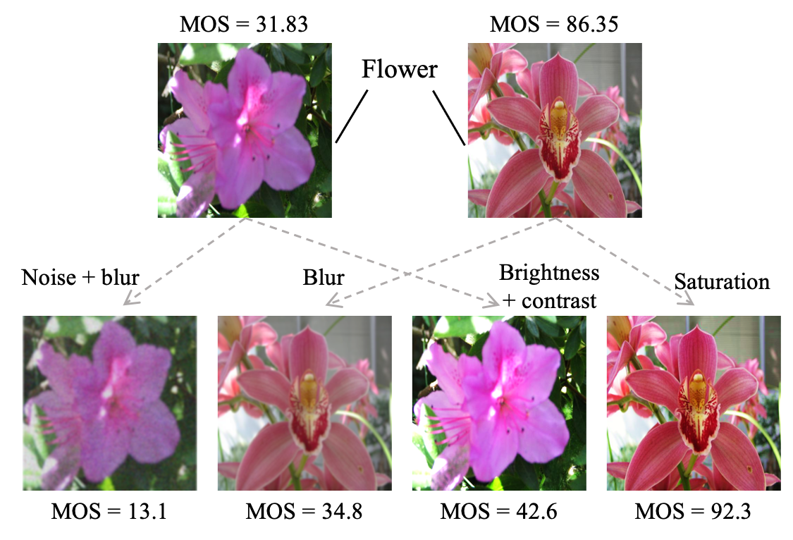
Researchers present several methods to tackle this challenge. A straight-forward way is to sample local patches and assign the label of the whole image (i.e., mean opinion score, MOS) to the patches [31, 4, 38, 89, 60, 90, 32]. However, the perceived scores of local image patches tend to differ from the score of the entire image [89, 79]. Another common strategy is to leverage domain knowledge from large-scale datasets (e.g., ImageNet [14]) for other computer vision tasks [32, 6]. Nevertheless, these pre-trained models can be sub-optimal for BIQA tasks: images with the same content share the same semantic label, whereas, their quality may be different (Fig. 1). Some researchers propose to train a model on synthetic images with artificial degradation and then regress the model onto small-scale target BIQA datasets[43, 89, 73]. However, images generated by rather simple degradation process with limited distortion types/levels are far from authentic. Further, synthetic images are regularly distorted from limited pristine images of high quality, so the image content itself only has a marginal effect on the image quality. Yet in real-world scenarios, the image quality is closely related to its content, due to viewers’ preferences for divergent contents [38, 62].

Self-supervised learning (SSL) or unsupervised learning is another potential choice to overcome the problem of lacking adequate training data, for its ability to utilize an amount of unlabeled data. Such technique is proven to be effective in many common computer vision tasks [2]. However, different from models for these tasks which mainly focus on high-level information, representations learned for BIQA should be sensitive to all kinds of low-level distortions and high-level contents, as well as interactions between them. There are few research focused on such area in the literature, let alone a deep SSL designed for BIQA with state-of-the-art performance [44].

In this work, we propose a novel SSL mechanism that distinguishes between samples with different perceptual qualities, generating Quality-aware Pre-Trained (QPT) models for downstream BIQA tasks. Specifically, we suppose the quality of patches from a distorted image should be similar, but vary from patches from different images (i.e., content-based negative) and the same image with different degradations (i.e., degradation-based negative). Moreover, inspired by recent progress in image restoration, we introduce shuffle order [84], high-order [70] and a skip operation to the image degradation process, to simulate real-world distortions. In this way, models pre-trained on ImageNet are expected to extract quality-aware features, and boost downstream BIQA performances. We summarize the contributions of this work as follows:

• We design a more complex degradation process suitable for BIQA. It not only considers a mixture of multiple degradation types, but also incorporates with shuffle order, high-order and a skip operation, resulting in a much larger degradation space. For a dataset with a size of $10^{7}$, our method can generate more than $2\times 10^{14}$ possible pairs for contrastive learning.

• To fully exploit the abundant information hidden beneath such an amount of data, we propose a novel SSL framework to generate QPT models for BIQA based on MoCoV2 [8]. By carefully designing positive/negative samples and customizing quality-aware contrastive loss, our approach enables models to learn quality-aware information rather than regular semantic-aware representation from massive unlabeled images.

• Extensive experiments on five BIQA benchmark datasets (sharing the same pre-trained weight of QPT) demonstrate that our proposed method significantly outperforms other counterparts, which indicates the effectiveness and generalization ability of QPT. It is also worth noting that the proposed method can be easily integrated with current SOTA methods by replacing their pre-trained weights.

2 Related Work

In this section, we provide a brief review of major works on BIQA and recent advances in contrastive learning and image degradation modeling.

2.1 Blind Image Quality Assessment

Before the rise of deep learning, natural scene statistics (NSS) theory dominates the realm of BIQA, which assumes that pristine natural images obey certain statistics distribution and various distortions will break such statistical regularity [59]. Based on this theory, various hand-crafted features are proposed in different domains, including spatial [47, 48], frequency [54, 49] and gradient [85]. Meanwhile, some learning-based methods [78, 46] have also been preliminarily explored. Typically, they estimate the subjective quality using support vector regression and features learned by visual codebooks [77].

In recent years, a variety of deep learning-based methods have been studied for BIQA and significantly boost the in-the-wild performance[28, 53, 67, 38, 21]. As a pioneer work, a shallow network [31] consisting of only three layers is built to solve BIQA in an end-to-end manner. After that, later works naturally expand the BIQA model by deepening the network depth [4, 42] or utilizing more effective building blocks [60, 91]. Recently, transformer-based BIQA methods [80, 92, 32, 76] are sprouting up, based on the assumption that transformer can compensate the missing ability of CNNs to capture non-local information [16].

Except for elaborate model design, a few research are devoted to solving the chief obstacle in BIQA, the paucity of labeled data. Some of them try to make full use of existing supervisory signals, such as rank learning [39, 37], multi-task learning [17] and mixed-dataset training [62, 90]. Meanwhile, others turn to large-scale pre-training [42, 82, 32], which generates a large number of distorted images labeled by specifications of degradation process [89] or quality scores estimated from FR models [43].

In comparison, our proposed method is based on contrastive learning without needing any explicit supervisory signal, thereby fully utilizing plenty of real-world images.

2.2 Self-supervised Learning

SSL, as a form of unsupervised learning, is used to learn a good data representation for the downstream true purpose [2]. A very straightforward idea to conduct such learning is minimizing the difference between a model’s output and a fixed target, such as reconstructing the input pixels [69] or predicting the pre-defined categories [15, 86]. Motivated by the successes of masked language modeling in natural language processing, masked image modeling [26, 75] is becoming a hot trend in computer vision.

Unlike the above methods, the goal of contrastive learning is to learn such an embedding space, where similar samples are assembled while dissimilar pairs are repelled [30]. Specifically, contrastive learning generally involves two aspects: pretext tasks and training objectives. Owing to the flexibility of contrastive learning, a wide range of pretext tasks have been proposed, such as colorization [86, 87], multi-view coding [64], and instance discrimination [74, 27]. When it comes to training objectives, the major trend is the move from only one positive and one negative sample [10, 55] to multiple positive and negative pairs [25, 66, 18]. Especially, InfoNCE [66] has become the most popular choice [27, 5, 9].

Notably, all of the above works can be classified as semantic-aware pre-training, because they encourage views (augmentations) of the same image to have a similar representation while ignoring the changes of perceived image quality. In this work, we redesign a quality-aware pretext task for BIQA, which will be discussed in Sec. 3.3.

2.3 Image Degradation Modelling

Most of the previous works focus on several classical distortion types [83, 72, 57, 56] to extract distortion-specific features. As the importance of BIQA is rising, more distortion types have been developed and applied to synthesize distorted images [40]. DipIQ [41] summarizes common distortion operations, such as noise, blur and compression, and further subdivides each with five levels. DB-CNN [89] introduces additional five distortion types. Recently, many works [34, 91, 21] point out that the above methods are too simple to simulate real-world images with complex and mixed distortions, due to the synthesized image only with a specific distortion type and level. In this work, we combine multiple degradation tricks [84, 70] proposed in the field of image restoration to form a much larger degradation space and generate distorted images that are more realistic.

3 Method

To excavate the potential of the “pre-training and fine-tuning” paradigm on BIQA for better performance, we present QPT models by pre-training on ImageNet. In Sec. 3.1, we will briefly review some related SSL frameworks. In Sec. 3.2, we will detail the degradation process for generating distorted images that contain quality-related information. In Sec. 3.3, we will give the definition of quality-aware pretext task and optimization objective.

Figure 2: Illustration of generating distorted images using different compositions of degradation. Compared with the process of fixed sequence, the introduced skip, shuffle and high-order largely increase the degradation space, covering diverse and realistic distortions.

3.1 Reviewing the Framework of SSL

SSL enables learning representations from orders of magnitude more data, which addresses the obstacle for BIQA in establishing large-scale annotated datasets. SSL methods can be roughly divided into generative-based [68, 26, 75] and contrastive-based [27, 7, 23]. Among them, MAE [26], as a generative-based method, develops an asymmetric encoder-decoder architecture for image reconstruction. MoCo [27], as a contrastive-based method, builds a dynamic dictionary with a queue and a moving-averaged encoder for contrastive learning. Relatively, contrastive learning is more suitable for BIQA, for which can easily measure quality ranking between samples. Due to the fact that the quality of an image is related to various complicated factors [65, 71], a large number of images are needed to ensure the diversity of negative samples [7]. Empirically, we choose MoCo, since it provides a memory-efficient framework to establish a large and consistent set.

In brief, MoCo builds a dictionary using a momentum queue to enlarge available size for comparison, where samples are progressively replaced with incoming mini-batch ones. And keys in the dictionary are updated through a momentum-based moving average of the encoder network, maintaining consistency with query samples. MoCo adopts the instance-level discrimination task [74] as its pretext task (i.e., a query matches a key if they are encoded views of the same image). Then, a contrastive loss, named InfoNCE, is adopted to distinguish the positive key from negative ones in a softmax manner, which can be noted as:

$$\mathcal{L}_{\text{InfoNCE}}=-\log\frac{\exp(q\cdot k_{+}/\tau)}{\sum_{i=0}^{N}\exp(q\cdot k_{i}/\tau)},$$ (1)

where $q$ is an encoded query, $k_{i}$ is the $i$-th encoded key of a dictionary consisting of $N$ samples, and $k_{+}$ is a single key that matches $q$. And $\tau$ is a temperature hyper-parameter.

3.2 Degradation Space

To obtain utilizable quality-related information in self-supervised scenarios, a simple way is to generate image pairs using controllable degradations manually. Before designing specific degradation types, several observations need to be mentioned: First, there exist many factors affecting the perceptual quality of an image (e.g., content, distortions, compression). For example, an image with unmeaningful content is often classified as a low-quality one [36]. Also, distortions (e.g., blurriness [13], noise [58] and sharpness [81]) introduced during the image production phase and compression artifacts introduced by transcoding or transmission, will degrade the overall quality. Second, the aforementioned factors, as a complicated composition, are always involved in practical scenarios [58, 1]. An image may go through various processes of shooting, editing, compression, and transmission, resulting in more complicated distortions. These scenarios increase the difficulty of BIQA tasks. Thus a good pre-trained model for IQA should take these into account, covering diverse distortions using suitable degradations as large and realistic as possible.

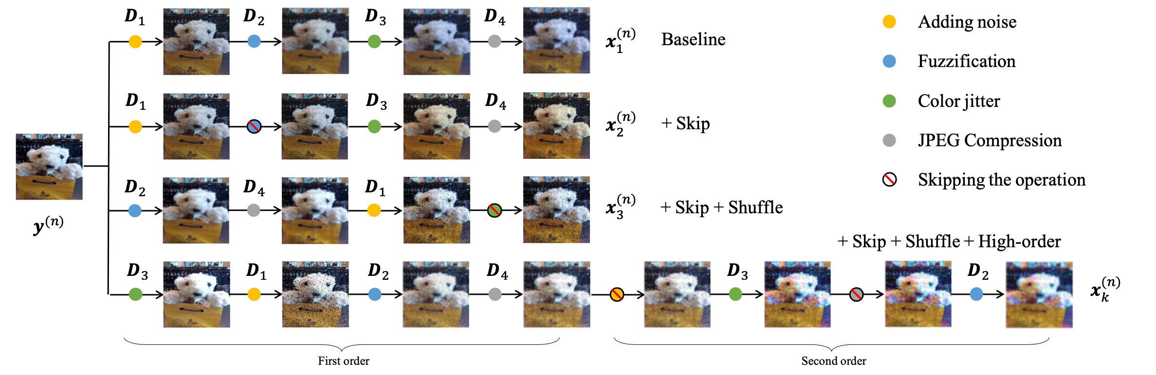
Based on these observations, we design the degradation space from the perspective of individual operations and their compositions. For the first observation, we introduce a variety of degradation types to simulate real distortions, which can be divided into three categories: (1) geometric deformation, which simulates distortions introduced during editing process or adaptation on various display equipment, including 4 operations of scale jitter [32], horizontal flip, down-sampling and up-sampling [50]; (2) color change [63], which can be caused by lightness, chroma, and hue differences in the shooting or codec process, including 2 operations of color jitter and grayscale; (3) texture adjustment, which can be captured from environmental interference or transmission, including 3 operations of adding noise, fuzzification [19] and JPEG compression [11]. Given an image $\mathbf{y}$, the process can be formulated as:

$$\mathbf{x}=\mathcal{D}(\mathbf{y};w,p),$$ (2)

where $\mathcal{D}$ denotes the function of degradation. $w$ represents hyper-parameters of the degradation (e.g., scale size, location, brightness intensity, etc.). And $p\in\{0,1\}$ indicates whether this operation is performed. For the second observation, we propose a sequence, consisting of randomly chosen degradations, for more complicated types (e.g., a list of {scale jitter, color jitter, adding noise}), where each operation can be skipped, and the order can be shuffled:

$$\mathbf{x}=\mathcal{D}^{o}(\mathbf{y})=\mathcal{D}_{o}(\cdots\mathcal{D}_{1}(\mathbf{y};w_{1},p_{1})\cdots;w_{o},p_{o}),$$ (3)

where $o$ is the number of selected degradations. Furthermore, to simulate multiple transfers, we adopt a high-order degradation type, involving multiple repeated processes of $\mathcal{D}^{o}(\mathbf{x})$, where each process performs with the same procedure but different hyper-parameters. Empirically, we employ a degenerate approach with at most two orders, as it could resolve most real cases while keeping simplicity. The illustration of the overall process is shown in Fig. 2.

The degradation space formed by our operations is much larger than those in existing super-resolution (SR) methods [70, 84], which reconstruct high-resolution images from low-resolution ones. Since BIQA does not require pixel-level aligned pairs like SR, more operations like geometric deformation/color change can be used. Moreover, SR requires that the source images should be high-quality and the distributions of target and source images should be as consistent as possible. These factors limit the number of available compositions. Without these restrictions, in our method, the size of degradation space can be expanded substantially. Theoretically, for a space containing 9 degradation types, the number of discrete compositions is $2\times\sum_{i=1}^{9}\mathbf{C}_{9}^{i}\times\mathbf{A}_{i}^{i}\thickapprox 2\times 10^{7}$.

Figure 3: The framework of Quality-aware Pretext Task (QPT). First, images are augmented by diverse degradations. Second, patches will be extracted from various views to form patch pairs. Pairs generated from the same view but different locations are treated as positive pairs. And other pairs are noted as negative pairs, including degradation-based and content-based. Then, the patches are transformed into encoded features by a network. Last, these feature pairs are constrained using a Quality-aware Contrastive Loss (QC-Loss).

3.3 Quality-aware Pretext Task

Different from the classical semantic-aware pretext task (i.e., treating each image instance as a distinct class) [74, 3], we propose a new quality-aware pretext task that distinguishes between samples with different perceptual qualities.

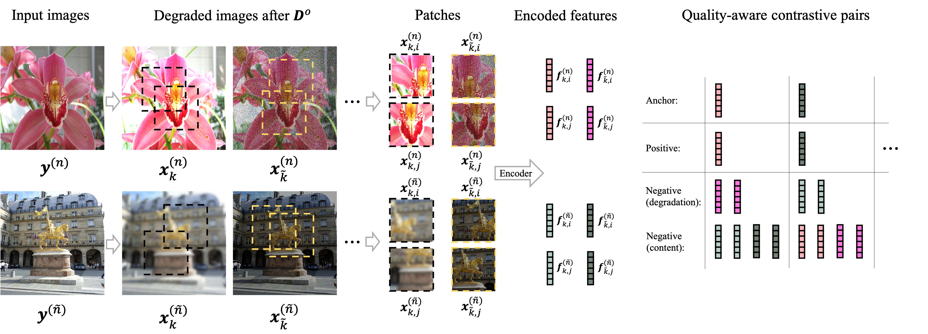
Suppose we have $N$ images $\mathbf{y}^{(1)},\cdots,\mathbf{y}^{(N)}$. As shown in Fig. 3, each image $\mathbf{y}^{(n)}$ will be differently augmented by $K$ degradation compositions, obtaining different “views” $\mathbf{x}^{(n)}_{1},\cdots,\mathbf{x}^{(n)}_{K}$ that own consistent content but with different perceptual qualities. Then we extract a “query” (or “anchor”) and a “key” patch that originates from the same view $\mathbf{x}^{(n)}_{k}$ but with different locations, denoted $\mathbf{x}^{(n)}_{k,i}$ and $\mathbf{x}^{(n)}_{k,j}$ respectively. The query and key are considered as a positive pair due to their consistent content and degradation type. And otherwise pairs are treated as negative ones, which can be divided into two parts. First, for the same image, patches extracted from different “views” are denoted as degradation-based negative pairs. Their content is the same, but the way it degenerates is different, resulting in inconsistent qualities. To ensure the quality of patches generated from a single image as consistent as possible, we set the lower bound for the area ratio during random crop to be 0.5. So patches generated from the same image share similar content rather than contrast regions (e.g., smooth and textured ones). Besides, for different images, regardless of whether their degradation types are the same, they are considered content-based negative pairs due to different contents. Notably, there may exist some noise (i.e., different contents, similar quality) under this partition, but it is negligible due to the very small proportions. To count the number of negative pairs with similar quality, we perform JND tests proposed in LPIPS [88] on 500 generated patches, indicating around 10%. Correctly assigned pairs still dominate. The difference between quality-level and instance-level discrimination tasks is given in Tab. 1.

Table 1: Comparison of two types of pretext tasks, where $\tilde{k}$ represents a degradation/augmentation type different from $k$, $\tilde{n}$ is an image different from $n$, and $\ast$ denotes an arbitrary value.

Pretext task	Positive Pair	Negative Pair
semantic-aware	$(\mathbf{x}^{(n)}_{k,i},\mathbf{x}^{(n)}_{\tilde{k},j})$	$(\mathbf{x}^{(n)}_{\ast,\ast},\mathbf{x}^{(\tilde{n})}_{\ast,\ast})$
quality-aware	$(\mathbf{x}^{(n)}_{k,i},\mathbf{x}^{(n)}_{k,j})$	$(\mathbf{x}^{(n)}_{\ast,\ast},\mathbf{x}^{(\tilde{n})}_{\ast,\ast})$, $(\mathbf{x}^{(n)}_{k,\ast},\mathbf{x}^{(n)}_{\tilde{k},\ast})$

Let $\mathcal{F}$ denote the transformation of the encoder network. Given an input patch $\mathbf{x}^{(n)}_{k,i}$, the encoded feature can be noted as $\mathbf{f}^{(n)}_{k,i}=\mathcal{F}(\mathbf{x}^{(n)}_{k,i})/||\mathcal{F}(\mathbf{x}^{(n)}_{k,i})||$, after a $\mathcal{L}_{2}$ normalization for computing the dot-product similarity. Then our method can be optimized using a Quality-aware Contrastive Loss (QC-Loss), which is formulated as follows:

$$\mathcal{L}_{\text{QC}}= -\beta\cdot\log\sum_{k=1}^{K}\frac{\exp(\mathbf{f}^{(n)}_{k,i}\cdot\mathbf{f}^{(n)}_{k,j}/\tau)}{\sum_{\tilde{k}\neq k}^{K}\exp(\mathbf{f}^{(n)}_{k,i}\cdot\mathbf{f}^{(n)}_{\tilde{k},j}/\tau)}$$ (4)

$$-\log\sum_{k=1}^{K}\frac{\exp(\mathbf{f}^{(n)}_{k,i}\cdot\mathbf{f}^{(n)}_{k,j}/\tau)}{\sum_{\tilde{n}\neq n}^{N}\sum_{k^{\prime}=1}^{K}\exp(\mathbf{f}^{(n)}_{k,i}\cdot\mathbf{f}^{(\tilde{n})}_{k^{\prime},j}/\tau)},$$

where the first part denotes distinguishing degradation-based negative pairs, and the second part is for content-based negative pairs. $\beta$ is a coefficient for balancing.

To further construct more image pairs containing abundant content and texture information, we adopt the well-known ImageNet as the baseline dataset for pre-training. Compared with IQA datasets, whose number of available data is relatively small (as shown in Tab. 2), ImageNet contains over 1 million of natural images from 1,000 diverse categories. Numerous samples and huge degradation space together contribute to generating $2\times 10^{14}$ possible pairs during the pre-training phase.

4 Experiments

4.1 Datasets and Evaluation Criteria

Datasets.

Our method is evaluated on five public BIQA datasets, including BID [12], CLIVE [20], KonIQ10K [29], SPAQ [17] and FLIVE [79]. BID is a blur image dataset that contains 586 images with realistic blur distortions (e.g., out-of-focus, simple motion, complex motion blur). CLIVE consists of 1,162 images with diverse authentic distortions captured by mobile devices. KonIQ10K contains 10,073 images which are selected from YFCC-100M. And the selected images cover a wide and uniform range of distortions in terms of quality indicators such as brightness, colorfulness, contrast, noise, sharpness, etc. SPAQ consists of 11,125 images captured by different mobile devices, covering a large variety of scene categories. FLIVE is the largest in-the-wild IQA dataset by far, which contains 39,810 real-world distorted images with diverse contents, sizes and aspect ratios. Details are given in Tab. 2.

Evaluation criteria.

Pearson’s Linear Correlation Coefficient (PLCC) and Spearman’s Rank-Order Correlation Coefficient (SRCC) are selected as criteria to measure the accuracy and monotonicity, respectively. They are in the range of [0, 1]. A larger PLCC means a more accurate numerical fit with MOS scores. A larger SRCC shows a more accurate ranking between samples. For all datasets, following [32, 21], we split the dataset into a 80% training set and a 20% testing set randomly.

Table 2: Details of selected BIQA datasets.

Dataset	Size	Resolution	MOS Range
BID [12]	586	480P$\sim$2112P	0$\sim$5
CLIVE [20]	1,162	500P$\sim$640P	0$\sim$100
KonIQ10K [29]	10,073	768P	0$\sim$100
SPAQ [17]	11,125	1080P$\sim$4368P	0$\sim$100
FLIVE [79]	39,810	160P$\sim$700P	0$\sim$100

Table 3: Performance of existing SOTA methods and the proposed QPT models on five in-the-wild BIQA datasets. The “$\star$” means missing corresponding results in the original paper. The best and second-best results are bolded and underlined. With the inherent learned knowledge in QPT models, a widely-used ResNet50 can outperform existing SOTA methods.

Method	BID		CLIVE		KonIQ10K		SPAQ		FLIVE
	SRCC	PLCC	SRCC	PLCC	SRCC	PLCC	SRCC	PLCC	SRCC	PLCC
NIQE [48]	0.4772	0.4713	0.4536	0.4676	0.5260	0.4745	0.6973	0.6850	0.1048	0.1409
ILNIQE [85]	0.4946	0.4538	0.4531	0.5114	0.5029	0.4956	0.7194	0.654	0.2188	0.2547
BRISQUE [47]	0.5736	0.5401	0.6005	0.6211	0.7150	0.7016	0.8021	0.8056	0.3201	0.3561
BMPRI [46]	0.5154	0.4583	0.4868	0.5229	0.6577	0.6546	0.7501	0.7544	0.2737	0.3146
CNNIQA [31]	0.6163	0.6144	0.6269	0.6008	0.6852	0.6837	0.7959	0.7988	0.3059	0.2850
WaDIQaM-NR [4]	0.6526	0.6359	0.6916	0.7304	0.7294	0.7538	0.8397	0.8449	0.4346	0.4303
SFA [38]	0.8202	0.8253	0.8037	0.8213	0.8882	0.8966	0.9057	0.9069	0.5415	0.6260
DB-CNN [89]	0.8450	0.8590	0.8443	0.8624	0.8780	0.8867	0.9099	0.9133	0.5537	0.6518
HyperIQA [60]	0.8544	0.8585	0.8546	0.8709	0.9075	0.9205	0.9155	0.9188	0.5354	0.6228
PaQ-2-PiQ⋆ [79]	-	-	0.840	0.850	0.870	0.880	-	-	0.571	0.623
CONRTIQUE⋆ [44]	-	-	0.854	0.890	0.896	0.901	-	-	0.580	0.641
UNIQUE⋆ [90]	0.858	0.873	0.854	0.890	0.896	0.901	-	-	-	-
MUSIQ⋆ [32]	-	-	-	-	0.916	0.928	0.917	0.921	0.566	0.661
TReS⋆ [21]	-	-	0.846	0.877	0.915	0.928	-	-	0.554	0.625
ResNet50	0.8423	0.8521	0.8527	0.8807	0.9121	0.9270	0.9161	0.9207	0.5514	0.6354
QPT-ResNet50	0.8875	0.9109	0.8947	0.9141	0.9271	0.9413	0.9250	0.9279	0.6104	0.6770

4.2 Implementation Details

Our experiments are performed using PyTorch [51], and are all conducted on 8 Nvidia V100 GPUs. Following the classical pre-training and fine-tuning paradigm, we run the whole experiments in two stages:

Pre-training.

We inherit most settings from MoCoV2 [8], while modify the pretext task and degradation process for the quality-aware purpose. Specifically, we use a ResNet50 [28] with an extra two-layer MLP as the encoder and train it on ImageNet. We use SGD optimizer with weight decay of 0.0001, momentum of 0.9 and a mini-batch size of 256. The initial learning rate is 0.03 and multiplied by 0.1 at 120 and 160 epoch. The hyper-parameters, $\beta$ and $\tau$ in Eq. 4, are empirically set to 0.4 and 0.2 in our experiments. It takes about 75 hours training ResNet50, for 200 epochs.

Fine-tuning.

Following the scheme from [62], we resize the smaller edge of images to 340 while maintaining aspect ratio, and randomly sample and horizontally flip patches with size 320x320 pixels. We use AdamW optimizer with weight decay of 0.01 and mini-batch size of 64. The Learning rate is initialized with 0.0002, and decayed by the cosine annealing strategy. For BID and CLIVE, experiments are trained for 100 epochs. And for other three dataset, the number is 200. By default, we select last epoch for weight initialization and evaluation. During test stage, we take five crops (i.e., four corners and a center patch) from an image, and average their corresponding prediction scores to get the final prediction score. To reduce the randomness in training/test set splitting, following [21, 60, 91], we repeat train/test procedures 10 times for each dataset, and report the median SRCC and PLCC results.

Table 4: Improving the performance of existing SOTA methods by replacing their pre-trained weights with QPT models directly. Experiments are conducted based on their open-source code, using the consistent dataset partitioning and training hyper-parameters.

Methods	Pre-trained Type	BID		CLIVE		KonIQ10K
		SRCC	PLCC	SRCC	PLCC	SRCC	PLCC
HyperIQA	Original	0.8665	0.8883	0.8553	0.8716	0.8990	0.9190
	QPT	0.8982+3.17%	0.9061 +1.78%	0.8743+1.90%	0.8732+0.16%	0.9066+0.76%	0.9241+0.51%
TRes	Original	0.7541	0.7918	0.8436	0.8793	0.8958	0.9097
	QPT	0.7936+3.95%	0.8037+1.19%	0.8666+2.30%	0.8882+0.89%	0.9052+0.94%	0.9150+0.53%

Table 5: Cross-dataset evaluation. Results of SRCC are reported.

Train	Test	DBCNN	HyperIQA	CONTRIQUE	QPT
KIQ10k	CLIVE	0.755	0.785	0.731	0.8208
KIQ10k	BID	0.816	0.819	-	0.8247
CLIVE	BID	0.762	0.756	-	0.8449
CLIVE	KIQ10k	0.754	0.772	0.676	0.7494

4.3 Comparison with SOTA BIQA Methods

We report the performance of SOTA BIQA methods in Tab. 3. Generally, our method pushes the current SOTA results a big step forward (using the same pre-trained weight generated by QPT), improving the best results to 0.8875 (+3.0%) of SRCC and 0.9109 (+4.6%) of PLCC in BID, 0.8947 (+4.0%) of SRCC and 0.9141 (+2.4%) of PLCC in CLIVE, 0.9271 (+1.1%) of SRCC and 0.9413 (+1.3%) of PLCC in KonIQ10K, 0.9250 (+0.8%) of SRCC and 0.9279 (+0.7%) of PLCC in SPAQ, and 0.5746 (+0.9%) of SRCC and 0.6748 (+1.4%) of PLCC in FLIVE. Notably, these results are achieved using an ordinary architecture of ResNet-50, showing the power of utilizing QPT models. Besides, we also report the results of naive ResNet-50 (i.e., using ImageNet supervised pre-training).

Specifically, QPT models surpass traditional methods (e.g., NIQE [48], ILNIQE [85], BRISQUE [47] and BMPRI [46]) that rely on hand-crafted features in large margins. Compared with earlier CNN-based methods (e.g., CNNIQA [31], WaDIQaM-NR [4] and SFA [38]), QPT shows the advantages of big data pre-training. For HyperIQA [60] that utilized a self-adaptive hyper network architecture to estimate content understanding, perception rule learning and quality predicting, QPT-ResNet50 obtains higher results without fine-designed architectures. Compared with current SOTA Transformer-based methods (e.g., MUSIQ [32] and TReS [21]), QPT models still outperform them, showing the effectiveness of quality-ware pretext training.

Due to the flexibility of QPT, it can be easily integrated with current SOTA methods by replacing their pre-trained weights. We reproduced two SOTA methods (i.e., HyperIQA and TReS) based on their official open-source code, giving the results in Tab. 4. The results of the comparison are based on a consistent dataset partitioning and training hyper-parameters, following official implementation. It can be seen that QPT further boosts SOTA methods effectively (e.g., a even better result with 0.8982 of SRCC in BID can be achieved), showing satisfactory generalization ability. We further give the corss-dataset evaluation in Tab. 5. Compared with the most competitive methods, QPT takes the lead in three scenarios.

4.4 Ablation Studies

Table 6: Impact of data amount for the pretext task of QPT, using different percentages of the ImageNet dataset, in BID and CLIVE.

Percentage of ImageNet	BID		CLIVE
	SRCC	PLCC	SRCC	PLCC
20%	0.8311	0.8305	0.8115	0.8203
50%	0.8760	0.8973	0.8868	0.9007
100%	0.8875	0.9109	0.8947	0.9141

Impact of data amount for QPT. To evaluate the effectiveness of the quality-aware pretext task, we use 20%, 50% and 100% percentages of the ImageNet dataset, analyzing the impact on the number of used data for downstream results. As given in Tab. 6, the larger the number used in the pre-training process, the better the performance on the downstream IQA datasets. Still, it is quite a surprise that our method obtains SOTA results with only 50% of the data. Furthermore, training larger-scale data is an open question and can be investigated in future work, where QPT may benefit from JFT-300M [61].

Table 7: Impact of encoder capacity for QPT, using different series of networks, in BID and CLIVE.

Network	Params	BID		CLIVE
		SRCC	PLCC	SRCC	PLCC
MBViTV2-100	4.90	0.8746	0.8799	0.8640	0.8914
MBViTV2-150	10.59	0.8782	0.8976	0.8702	0.8970
MBViTV2-200	18.45	0.8821	0.8960	0.8894	0.9006
ResNet-18	11.69	0.8679	0.8805	0.8610	0.8795
ResNet-34	21.80	0.8742	0.9001	0.8780	0.8871
ResNet-50	25.56	0.8875	0.9109	0.8947	0.9141

Impact of encoder capacity for QPT. To verify the effect of model capacity on feature modeling, we select two series of networks for analysis, including the widely-used CNN architectures of ResNet and an emerging Transformer-based architectures of MobileViTV2 [45]. As shown in Tab. 7, increasing the model size can help improve the ability of feature representation, resulting in better downstream performance. It should be pointed out that large models will also increase the time consumption of the pre-training phase (i.e., ResNets of {53h, 61h, 75h}, MBViTV2s of {66h, 92h, 109h}, respectively). We did not use larger networks out of tradeoffs, which can be tried in future work.

Table 8: Impact on the composition of negative samples.

Inter	Intra	BID		CLIVE
		SRCC	PLCC	SRCC	PLCC
✓	✓	0.8875	0.9109	0.8947	0.9141
✓	$\times$	0.8702	0.9051	0.8721	0.8994
$\times$	✓	0.8399	0.8357	0.8084	0.8142
$\times$	$\times$	0.7078	0.7731	0.7495	0.7493

Impact of different compositions of negative samples. To evaluate the effectiveness of negative samples and the proposed QC Loss, we give the results in Tab. 8. The highest result is achieved when both types of negative samples are present. And the absence of inter-sample negative pairs leads to a larger performance drop. This is due to the fact that compared with intra-sample negative pairs (i.e., $K-1$), the number of inter-sample ones (i.e., $N\cdot K$), which contain both different content and degradation types, is larger.

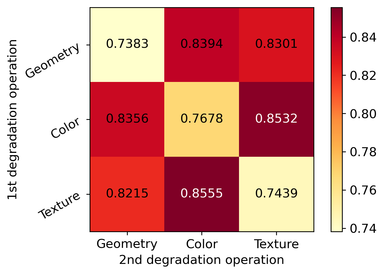
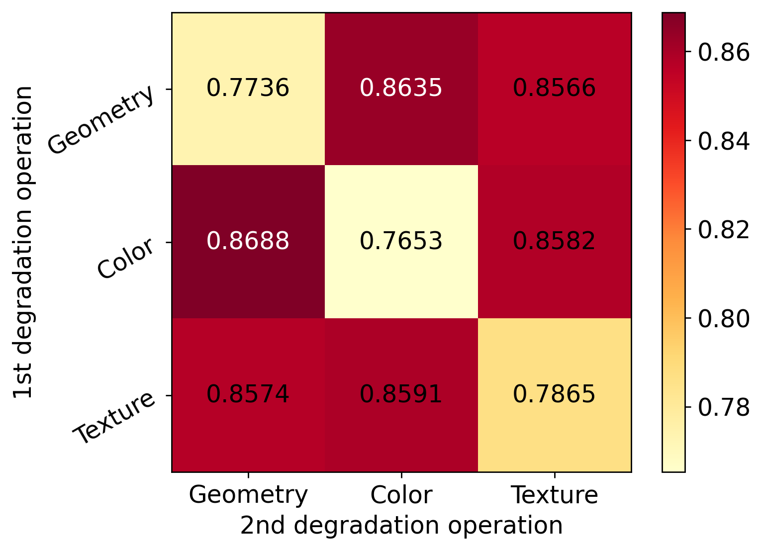
Ablation on the degradation space. Experiments are performed to evaluate the impact of different degradations and compositions. In Fig. 4, we give the results under different compositions of degradation types in a first-order manner. Trying all combinations is impractical due to the huge degradation space. Experiments are performed in a coarse-grained manner. The results show that there is a clear effect difference between the degradation types of a fixed form. More flexible and larger space are needed to cover different downstream scenarios. We further evaluate the strategy of composition as shown in Fig. 2. In Tab. 9, a combination of the three strategies yielded the best results.

(a) Results in BID

(b) Results in CLIVE

Figure 4: Evaluation results of SRCC under different fixed compositions of degradations in a first-order manner. The diagonal entries denote single class degradation type, and off-diagonals represent composition of two-class degradation applied sequentially.

Table 9: Ablation on the degradation space (different formulation type in Eq. 3 of complicated degradation models) in BID.

skip	shuffle	two-order	SRCC	PLCC
✓	✓	✓	0.8875	0.9109
✓	✓	$\times$	0.8828	0.9075
✓	$\times$	$\times$	0.8745	0.9029
$\times$	$\times$	$\times$	0.8626	0.8864

4.5 Comparisons with other pretext tasks

We further compare QPT with other pretext methods, including train-from-scratch (i.e., w/o pre-training weights), supervised and MoCo. We extract features from the encoder output for both fine-tuning and linear probing evaluations.

Table 10: Comparisons of linear probing evaluation using different pretext tasks in BID and CLIVE.

Pretext task	BID		CLIVE
	SRCC	PLCC	SRCC	PLCC
Supervised	0.7678	0.7860	0.7128	0.7668
MoCo	0.7367	0.7357	0.6796	0.7154
QPT	0.8242	0.8175	0.7613	0.7938

Linear probing evaluation. In this way, the weights of encoder are frozen for feature extraction directly. As given in Tab. 10, QPT obtains the best performance, surpassing MoCo by 8.75% of SRCC in BID and 8.17% in CLIVE.

Table 11: Comparisons of end-to-end fine-tuning evaluation using different pretext tasks in BID and CLIVE.

Pretext task	BID		CLIVE
	SRCC	PLCC	SRCC	PLCC
w/o	0.7078	0.7731	0.7495	0.7493
Supervised	0.8423	0.8521	0.8527	0.8807
MoCo	0.8531	0.8724	0.8494	0.8615
QPT	0.8875	0.9109	0.8947	0.9141

End-to-end fine-tuning evaluation. Linear probing has been a popular protocol in the past few years. However, it misses the opportunity of pursuing strong but nonlinear features which is indeed a strength of deep learning [26]. We also give the fine-tuning results in Tab. 11. QPT still achieves the best results. Generally, higher results can be obtained than linear probing. These results further prove the effectiveness of QPT over instance-level discrimination or supervised classification pretext tasks in IQA scenarios.

5 Conclusion

In this paper, we proposed the QPT to generate pre-trained models for downstream BIQA tasks, alleviating the obstacle of insufficient annotated data. By introducing diverse degradation types and compositions, we construct a degradation space that contains $2\times 10^{7}$ possible degradations, to simulate more complicated and realistic distorted images. To constrain the learning process, we proposed the QC-Loss that treats patch pairs extracted from the same degraded images as positive ones. And other pairs are noted as negative ones, including degradation-based and content-based ones. After pre-trained on ImageNet using QPT, BIQA models obtain significant improvements on five BIQA benchmark datasets. Moreover, QPT can be easily integrated with current SOTA methods by replacing their pre-trained weights, showing good generalization ability.

References

- [1] Sewoong Ahn, Yeji Choi, and Kwangjin Yoon. Deep learning-based distortion sensitivity prediction for full-reference image quality assessment. In CVPR Workshops, pages 344–353. Computer Vision Foundation / IEEE, 2021.
- [2] Saleh Albelwi. Survey on self-supervised learning: Auxiliary pretext tasks and contrastive learning methods in imaging. Entropy, 24(4):551, 2022.
- [3] Philip Bachman, R. Devon Hjelm, and William Buchwalter. Learning representations by maximizing mutual information across views. In NeurIPS, pages 15509–15519, 2019.
- [4] Sebastian Bosse, Dominique Maniry, Klaus-Robert Müller, Thomas Wiegand, and Wojciech Samek. Deep neural networks for no-reference and full-reference image quality assessment. IEEE Trans. Image Process., 27(1):206–219, 2018.
- [5] Mathilde Caron, Ishan Misra, Julien Mairal, Priya Goyal, Piotr Bojanowski, and Armand Joulin. Unsupervised learning of visual features by contrasting cluster assignments. In NeurIPS, 2020.
- [6] Pengfei Chen, Leida Li, Jinjian Wu, Weisheng Dong, and Guangming Shi. Contrastive self-supervised pre-training for video quality assessment. IEEE Trans. Image Process., 31:458–471, 2022.
- [7] Ting Chen, Simon Kornblith, Mohammad Norouzi, and Geoffrey E. Hinton. A simple framework for contrastive learning of visual representations. In ICML, volume 119 of Proceedings of Machine Learning Research, pages 1597–1607. PMLR, 2020.
- [8] Xinlei Chen, Haoqi Fan, Ross B. Girshick, and Kaiming He. Improved baselines with momentum contrastive learning. CoRR, abs/2003.04297, 2020.
- [9] Xinlei Chen, Saining Xie, and Kaiming He. An empirical study of training self-supervised vision transformers. In ICCV, pages 9620–9629. IEEE, 2021.
- [10] Sumit Chopra, Raia Hadsell, and Yann LeCun. Learning a similarity metric discriminatively, with application to face verification. In CVPR (1), pages 539–546. IEEE Computer Society, 2005.
- [11] Li Sze Chow and Raveendran Paramesran. Review of medical image quality assessment. Biomed. Signal Process. Control., 27:145–154, 2016.
- [12] Alexandre G. Ciancio, André Luiz N. Targino da Costa, Eduardo A. B. da Silva, Amir Said, Ramin Samadani, and Pere Obrador. No-reference blur assessment of digital pictures based on multifeature classifiers. IEEE Trans. Image Process., 20(1):64–75, 2011.
- [13] Erez Cohen and Yitzhak Yitzhaky. No-reference assessment of blur and noise impacts on image quality. Signal Image Video Process., 4(3):289–302, 2010.
- [14] Jia Deng, Wei Dong, Richard Socher, Li-Jia Li, Kai Li, and Li Fei-Fei. Imagenet: A large-scale hierarchical image database. In CVPR, pages 248–255. IEEE Computer Society, 2009.
- [15] Carl Doersch, Abhinav Gupta, and Alexei A. Efros. Unsupervised visual representation learning by context prediction. In ICCV, pages 1422–1430. IEEE Computer Society, 2015.
- [16] Alexey Dosovitskiy, Lucas Beyer, Alexander Kolesnikov, Dirk Weissenborn, Xiaohua Zhai, Thomas Unterthiner, Mostafa Dehghani, Matthias Minderer, Georg Heigold, Sylvain Gelly, Jakob Uszkoreit, and Neil Houlsby. An image is worth 16x16 words: Transformers for image recognition at scale. In ICLR. OpenReview.net, 2021.
- [17] Yuming Fang, Hanwei Zhu, Yan Zeng, Kede Ma, and Zhou Wang. Perceptual quality assessment of smartphone photography. In CVPR, pages 3674–3683. Computer Vision Foundation / IEEE, 2020.
- [18] Nicholas Frosst, Nicolas Papernot, and Geoffrey E. Hinton. Analyzing and improving representations with the soft nearest neighbor loss. In ICML, volume 97 of Proceedings of Machine Learning Research, pages 2012–2020. PMLR, 2019.
- [19] Yixuan Gao, Xiongkuo Min, Yucheng Zhu, Jing Li, Xiao-Ping Zhang, and Guangtao Zhai. Image quality assessment: From mean opinion score to opinion score distribution. In ACM Multimedia, pages 997–1005. ACM, 2022.
- [20] Deepti Ghadiyaram and Alan C. Bovik. Massive online crowdsourced study of subjective and objective picture quality. IEEE Trans. Image Process., 25(1):372–387, 2016.
- [21] S. Alireza Golestaneh, Saba Dadsetan, and Kris M. Kitani. No-reference image quality assessment via transformers, relative ranking, and self-consistency. In WACV, pages 3989–3999. IEEE, 2022.
- [22] S. Alireza Golestaneh and Lina J. Karam. Reduced-reference quality assessment based on the entropy of DWT coefficients of locally weighted gradient magnitudes. IEEE Trans. Image Process., 25(11):5293–5303, 2016.
- [23] Jean-Bastien Grill, Florian Strub, Florent Altché, Corentin Tallec, Pierre H. Richemond, Elena Buchatskaya, Carl Doersch, Bernardo Ávila Pires, Zhaohan Guo, Mohammad Gheshlaghi Azar, Bilal Piot, Koray Kavukcuoglu, Rémi Munos, and Michal Valko. Bootstrap your own latent - A new approach to self-supervised learning. In NeurIPS, 2020.
- [24] Ke Gu, Dacheng Tao, Junfei Qiao, and Weisi Lin. Learning a no-reference quality assessment model of enhanced images with big data. IEEE Trans. Neural Networks Learn. Syst., 29(4):1301–1313, 2018.
- [25] Michael Gutmann and Aapo Hyvärinen. Noise-contrastive estimation: A new estimation principle for unnormalized statistical models. In AISTATS, volume 9 of JMLR Proceedings, pages 297–304. JMLR.org, 2010.
- [26] Kaiming He, Xinlei Chen, Saining Xie, Yanghao Li, Piotr Dollár, and Ross B. Girshick. Masked autoencoders are scalable vision learners. In CVPR, pages 15979–15988. IEEE, 2022.
- [27] Kaiming He, Haoqi Fan, Yuxin Wu, Saining Xie, and Ross B. Girshick. Momentum contrast for unsupervised visual representation learning. In CVPR, pages 9726–9735. Computer Vision Foundation / IEEE, 2020.
- [28] Kaiming He, Xiangyu Zhang, Shaoqing Ren, and Jian Sun. Deep residual learning for image recognition. In CVPR, pages 770–778. IEEE Computer Society, 2016.
- [29] Vlad Hosu, Hanhe Lin, Tamás Szirányi, and Dietmar Saupe. Koniq-10k: An ecologically valid database for deep learning of blind image quality assessment. IEEE Trans. Image Process., 29:4041–4056, 2020.
- [30] Ashish Jaiswal, Ashwin Ramesh Babu, Mohammad Zaki Zadeh, Debapriya Banerjee, and Fillia Makedon. A survey on contrastive self-supervised learning. CoRR, abs/2011.00362, 2020.
- [31] Le Kang, Peng Ye, Yi Li, and David S. Doermann. Convolutional neural networks for no-reference image quality assessment. In CVPR, pages 1733–1740. IEEE Computer Society, 2014.
- [32] Junjie Ke, Qifei Wang, Yilin Wang, Peyman Milanfar, and Feng Yang. MUSIQ: multi-scale image quality transformer. In ICCV, pages 5128–5137. IEEE, 2021.
- [33] Jongyoo Kim and Sanghoon Lee. Deep learning of human visual sensitivity in image quality assessment framework. In CVPR, pages 1969–1977. IEEE Computer Society, 2017.
- [34] Jongyoo Kim, Hui Zeng, Deepti Ghadiyaram, Sanghoon Lee, Lei Zhang, and Alan C. Bovik. Deep convolutional neural models for picture-quality prediction: Challenges and solutions to data-driven image quality assessment. IEEE Signal Process. Mag., 34(6):130–141, 2017.
- [35] Alex Krizhevsky, Geoffrey Hinton, et al. Learning multiple layers of features from tiny images. 2009.
- [36] Dingquan Li, Tingting Jiang, and Ming Jiang. Quality assessment of in-the-wild videos. In ACM Multimedia, pages 2351–2359. ACM, 2019.
- [37] Dingquan Li, Tingting Jiang, and Ming Jiang. Norm-in-norm loss with faster convergence and better performance for image quality assessment. In ACM Multimedia, pages 789–797. ACM, 2020.
- [38] Dingquan Li, Tingting Jiang, Weisi Lin, and Ming Jiang. Which has better visual quality: The clear blue sky or a blurry animal? IEEE Trans. Multim., 21(5):1221–1234, 2019.
- [39] Xialei Liu, Joost van de Weijer, and Andrew D. Bagdanov. Rankiqa: Learning from rankings for no-reference image quality assessment. In ICCV, pages 1040–1049. IEEE Computer Society, 2017.
- [40] Kede Ma, Zhengfang Duanmu, Qingbo Wu, Zhou Wang, Hongwei Yong, Hongliang Li, and Lei Zhang. Waterloo exploration database: New challenges for image quality assessment models. IEEE Trans. Image Process., 26(2):1004–1016, 2017.
- [41] Kede Ma, Wentao Liu, Tongliang Liu, Zhou Wang, and Dacheng Tao. dipiq: Blind image quality assessment by learning-to-rank discriminable image pairs. IEEE Trans. Image Process., 26(8):3951–3964, 2017.
- [42] Kede Ma, Wentao Liu, Kai Zhang, Zhengfang Duanmu, Zhou Wang, and Wangmeng Zuo. End-to-end blind image quality assessment using deep neural networks. IEEE Trans. Image Process., 27(3):1202–1213, 2018.
- [43] Kede Ma, Xuelin Liu, Yuming Fang, and Eero P. Simoncelli. Blind image quality assessment by learning from multiple annotators. In ICIP, pages 2344–2348. IEEE, 2019.
- [44] Pavan C. Madhusudana, Neil Birkbeck, Yilin Wang, Balu Adsumilli, and Alan C. Bovik. Image quality assessment using contrastive learning. IEEE Trans. Image Process., 31:4149–4161, 2022.
- [45] Sachin Mehta and Mohammad Rastegari. Separable self-attention for mobile vision transformers. CoRR, abs/2206.02680, 2022.
- [46] Xiongkuo Min, Guangtao Zhai, Ke Gu, Yutao Liu, and Xiaokang Yang. Blind image quality estimation via distortion aggravation. IEEE Trans. Broadcast., 64(2):508–517, 2018.
- [47] Anish Mittal, Anush Krishna Moorthy, and Alan Conrad Bovik. No-reference image quality assessment in the spatial domain. IEEE Trans. Image Process., 21(12):4695–4708, 2012.
- [48] Anish Mittal, Rajiv Soundararajan, and Alan C. Bovik. Making a ”completely blind” image quality analyzer. IEEE Signal Process. Lett., 20(3):209–212, 2013.
- [49] Anush K. Moorthy and Alan Conrad Bovik. Blind image quality assessment: From natural scene statistics to perceptual quality. IEEE Trans. Image Process., 20(12):3350–3364, 2011.
- [50] Fu-Zhao Ou, Yuan-Gen Wang, and Guopu Zhu. A novel blind image quality assessment method based on refined natural scene statistics. In ICIP, pages 1004–1008. IEEE, 2019.
- [51] Adam Paszke, Sam Gross, Francisco Massa, Adam Lerer, James Bradbury, Gregory Chanan, Trevor Killeen, Zeming Lin, Natalia Gimelshein, Luca Antiga, Alban Desmaison, Andreas Köpf, Edward Z. Yang, Zachary DeVito, Martin Raison, Alykhan Tejani, Sasank Chilamkurthy, Benoit Steiner, Lu Fang, Junjie Bai, and Soumith Chintala. Pytorch: An imperative style, high-performance deep learning library. In NeurIPS, pages 8024–8035, 2019.
- [52] Abdul Rehman and Zhou Wang. Reduced-reference image quality assessment by structural similarity estimation. IEEE Trans. Image Process., 21(8):3378–3389, 2012.
- [53] Shaoqing Ren, Kaiming He, Ross B. Girshick, and Jian Sun. Faster R-CNN: towards real-time object detection with region proposal networks. In NIPS, pages 91–99, 2015.
- [54] Michele A. Saad, Alan C. Bovik, and Christophe Charrier. Blind image quality assessment: A natural scene statistics approach in the DCT domain. IEEE Trans. Image Process., 21(8):3339–3352, 2012.
- [55] Florian Schroff, Dmitry Kalenichenko, and James Philbin. Facenet: A unified embedding for face recognition and clustering. In CVPR, pages 815–823. IEEE Computer Society, 2015.
- [56] Hamid R. Sheikh, Alan C. Bovik, and Lawrence K. Cormack. No-reference quality assessment using natural scene statistics: JPEG2000. IEEE Trans. Image Process., 14(11):1918–1927, 2005.
- [57] Hamid R. Sheikh, Zhou Wang, and Alan C. Bovik. No-reference perceptual quality assessment of JPEG compressed images. In ICIP (1), pages 477–480. IEEE, 2002.
- [58] Ji Shen, Qin Li, and Gordon Erlebacher. Hybrid no-reference natural image quality assessment of noisy, blurry, jpeg2000, and JPEG images. IEEE Trans. Image Process., 20(8):2089–2098, 2011.
- [59] Eero P Simoncelli and Bruno A Olshausen. Natural image statistics and neural representation. Annual review of neuroscience, 24(1):1193–1216, 2001.
- [60] Shaolin Su, Qingsen Yan, Yu Zhu, Cheng Zhang, Xin Ge, Jinqiu Sun, and Yanning Zhang. Blindly assess image quality in the wild guided by a self-adaptive hyper network. In CVPR, pages 3664–3673. Computer Vision Foundation / IEEE, 2020.
- [61] Chen Sun, Abhinav Shrivastava, Saurabh Singh, and Abhinav Gupta. Revisiting unreasonable effectiveness of data in deep learning era. In ICCV, pages 843–852. IEEE Computer Society, 2017.
- [62] Wei Sun, Xiongkuo Min, Guangtao Zhai, and Siwei Ma. Blind quality assessment for in-the-wild images via hierarchical feature fusion and iterative mixed database training. CoRR, abs/2105.14550, 2021.
- [63] Dogancan Temel and Ghassan AlRegib. CSV: image quality assessment based on color, structure, and visual system. Signal Process. Image Commun., 48:92–103, 2016.
- [64] Yonglong Tian, Dilip Krishnan, and Phillip Isola. Contrastive multiview coding. In ECCV (11), volume 12356 of Lecture Notes in Computer Science, pages 776–794. Springer, 2020.
- [65] Zhengzhong Tu, Yilin Wang, Neil Birkbeck, Balu Adsumilli, and Alan C. Bovik. UGC-VQA: benchmarking blind video quality assessment for user generated content. IEEE Trans. Image Process., 30:4449–4464, 2021.
- [66] Aäron van den Oord, Yazhe Li, and Oriol Vinyals. Representation learning with contrastive predictive coding. CoRR, abs/1807.03748, 2018.
- [67] Ashish Vaswani, Noam Shazeer, Niki Parmar, Jakob Uszkoreit, Llion Jones, Aidan N. Gomez, Lukasz Kaiser, and Illia Polosukhin. Attention is all you need. In NIPS, pages 5998–6008, 2017.
- [68] Pascal Vincent, Hugo Larochelle, Yoshua Bengio, and Pierre-Antoine Manzagol. Extracting and composing robust features with denoising autoencoders. In ICML, volume 307 of ACM International Conference Proceeding Series, pages 1096–1103. ACM, 2008.
- [69] Pascal Vincent, Hugo Larochelle, Isabelle Lajoie, Yoshua Bengio, and Pierre-Antoine Manzagol. Stacked denoising autoencoders: Learning useful representations in a deep network with a local denoising criterion. J. Mach. Learn. Res., 11:3371–3408, 2010.
- [70] Xintao Wang, Liangbin Xie, Chao Dong, and Ying Shan. Real-esrgan: Training real-world blind super-resolution with pure synthetic data. In ICCVW, pages 1905–1914. IEEE, 2021.
- [71] Yilin Wang, Junjie Ke, Hossein Talebi, Joong Gon Yim, Neil Birkbeck, Balu Adsumilli, Peyman Milanfar, and Feng Yang. Rich features for perceptual quality assessment of UGC videos. In CVPR, pages 13435–13444. Computer Vision Foundation / IEEE, 2021.
- [72] Zhou Wang and Eero P. Simoncelli. Local phase coherence and the perception of blur. In NIPS, pages 1435–1442. MIT Press, 2003.
- [73] Jinjian Wu, Jupo Ma, Fuhu Liang, Weisheng Dong, Guangming Shi, and Weisi Lin. End-to-end blind image quality prediction with cascaded deep neural network. IEEE Trans. Image Process., 29:7414–7426, 2020.
- [74] Zhirong Wu, Yuanjun Xiong, Stella X. Yu, and Dahua Lin. Unsupervised feature learning via non-parametric instance discrimination. In CVPR, pages 3733–3742. Computer Vision Foundation / IEEE Computer Society, 2018.
- [75] Zhenda Xie, Zheng Zhang, Yue Cao, Yutong Lin, Jianmin Bao, Zhuliang Yao, Qi Dai, and Han Hu. Simmim: a simple framework for masked image modeling. In CVPR, pages 9643–9653. IEEE, 2022.
- [76] Sidi Yang, Tianhe Wu, Shuwei Shi, Shanshan Lao, Yuan Gong, Mingdeng Cao, Jiahao Wang, and Yujiu Yang. MANIQA: multi-dimension attention network for no-reference image quality assessment. In CVPR Workshops, pages 1190–1199. IEEE, 2022.
- [77] Peng Ye and David S. Doermann. No-reference image quality assessment using visual codebooks. IEEE Trans. Image Process., 21(7):3129–3138, 2012.
- [78] Peng Ye, Jayant Kumar, Le Kang, and David S. Doermann. Unsupervised feature learning framework for no-reference image quality assessment. In CVPR, pages 1098–1105. IEEE Computer Society, 2012.
- [79] Zhenqiang Ying, Haoran Niu, Praful Gupta, Dhruv Mahajan, Deepti Ghadiyaram, and Alan C. Bovik. From patches to pictures (paq-2-piq): Mapping the perceptual space of picture quality. In CVPR, pages 3572–3582. Computer Vision Foundation / IEEE, 2020.
- [80] Junyong You and Jari Korhonen. Transformer for image quality assessment. In ICIP, pages 1389–1393. IEEE, 2021.
- [81] Guanghui Yue, Chunping Hou, Ke Gu, Tianwei Zhou, and Guangtao Zhai. Combining local and global measures for dibr-synthesized image quality evaluation. IEEE Trans. Image Process., 28(4):2075–2088, 2019.
- [82] Hui Zeng, Lei Zhang, and Alan C. Bovik. Blind image quality assessment with a probabilistic quality representation. In ICIP, pages 609–613. IEEE, 2018.
- [83] Jian Zhang, Ruiqin Xiong, Chen Zhao, Siwei Ma, and Debin Zhao. Exploiting image local and nonlocal consistency for mixed gaussian-impulse noise removal. CoRR, abs/1208.3718, 2012.
- [84] Kai Zhang, Jingyun Liang, Luc Van Gool, and Radu Timofte. Designing a practical degradation model for deep blind image super-resolution. In ICCV, pages 4771–4780. IEEE, 2021.
- [85] Lin Zhang, Lei Zhang, and Alan C. Bovik. A feature-enriched completely blind image quality evaluator. IEEE Trans. Image Process., 24(8):2579–2591, 2015.
- [86] Richard Zhang, Phillip Isola, and Alexei A. Efros. Colorful image colorization. In ECCV (3), volume 9907 of Lecture Notes in Computer Science, pages 649–666. Springer, 2016.
- [87] Richard Zhang, Phillip Isola, and Alexei A. Efros. Split-brain autoencoders: Unsupervised learning by cross-channel prediction. In CVPR, pages 645–654. IEEE Computer Society, 2017.
- [88] Richard Zhang, Phillip Isola, Alexei A. Efros, Eli Shechtman, and Oliver Wang. The unreasonable effectiveness of deep features as a perceptual metric. In CVPR, pages 586–595. Computer Vision Foundation / IEEE Computer Society, 2018.
- [89] Weixia Zhang, Kede Ma, Jia Yan, Dexiang Deng, and Zhou Wang. Blind image quality assessment using a deep bilinear convolutional neural network. IEEE Trans. Circuits Syst. Video Technol., 30(1):36–47, 2020.
- [90] Weixia Zhang, Kede Ma, Guangtao Zhai, and Xiaokang Yang. Uncertainty-aware blind image quality assessment in the laboratory and wild. IEEE Trans. Image Process., 30:3474–3486, 2021.
- [91] Hancheng Zhu, Leida Li, Jinjian Wu, Weisheng Dong, and Guangming Shi. Metaiqa: Deep meta-learning for no-reference image quality assessment. In CVPR, pages 14131–14140. Computer Vision Foundation / IEEE, 2020.
- [92] Mengmeng Zhu, Guanqun Hou, Xinjia Chen, Jiaxing Xie, Haixian Lu, and Jun Che. Saliency-guided transformer network combined with local embedding for no-reference image quality assessment. In ICCVW, pages 1953–1962. IEEE, 2021.