Fast and Interpretable Dynamics for Fisher Markets
via Block-Coordinate Updates

Abstract

We consider the problem of large-scale Fisher market equilibrium computation through scalable first-order optimization methods. It is well-known that market equilibria can be captured using structured convex programs such as the Eisenberg-Gale and Shmyrev convex programs. Highly performant deterministic full-gradient first-order methods have been developed for these programs. In this paper, we develop new block-coordinate first-order methods for computing Fisher market equilibria, and show that these methods have interpretations as tâtonnement-style or proportional response-style dynamics where either buyers or items show up one at a time. We reformulate these convex programs and solve them using proximal block coordinate descent methods, a class of methods that update only a small number of coordinates of the decision variable in each iteration. Leveraging recent advances in the convergence analysis of these methods and structures of the equilibrium-capturing convex programs, we establish fast convergence rates of these methods.

1 Introduction

In a market equilibrium (ME) a set of items is allocated to a set of buyers via a set of prices for the items and an allocation of items to buyers such that each buyer spends their budget optimally, and all items are fully allocated. Due to its rich structural properties and strong fairness and efficiency guarantees, ME has long been used to develop fair division and online resource allocation mechanisms (Gao and Kroer 2021; Aziz and Ye 2014; Barman, Krishnamurthy, and Vaish 2018; Arnsperger 1994). Market model and corresponding equilibrium computation algorithms have been central research topics in market design and related areas in economics, computer science and operations research with practical impacts (Scarf et al. 1967; Kantorovich 1975; Othman, Sandholm, and Budish 2010; Daskalakis, Goldberg, and Papadimitriou 2009; Cole et al. 2017; Kroer et al. 2019). More specifically, many works in market design rely on the assumption that ME can be computed efficiently for large-scale market instances. For example, the well-known fair division mechanism without money competitive equilibrium from equal incomes (CEEI) requires computing a ME of a Fisher market under uniform buyer budgets (Varian et al. 1974). Recent work has also established close connections between market equilibria and important solution concepts in the context of large-scale Internet markets, such as pacing equilibria in repeated auctions (Conitzer et al. 2018, 2019; Kroer and Stier-Moses 2022). Motivated by the classical and emerging applications described above, we are interested in developing efficient equilibrium computation algorithms for large-scale market instances. In general, computing a ME is a hard problem (Chen and Teng 2009; Vazirani and Yannakakis 2011; Othman, Papadimitriou, and Rubinstein 2016). However, for the case of Fisher markets and certain classes of utility functions, efficient algorithms are known (Devanur et al. 2008; Zhang 2011; Gao and Kroer 2020), often based on solving a specific convex program—whose solutions are ME and vice versa—using an optimization algorithm. In this paper, we focus on two well-known such convex programs, namely, the Eisenberg-Gale (EG) (Eisenberg and Gale 1959; Eisenberg 1961) and Shmyrev convex programs (Shmyrev 2009; Cole et al. 2017).

Most existing equilibrium computation literature studies the case of a static market where all buyers and items are present in every time step of the equilibrium computation process. In contrast, we study a setting where only a random subset of buyer-item pairs show up at each time step. Such a setting is well-motivated from a computational perspective, since stochastic methods are typically more efficient for extremely large problems. Secondly, our model allows us to model new types of market dynamics. We make use of recent advances in stochastic first-order optimization, more specifically, block-coordinate-type methods, to design new equilibrium computation algorithms for this setting. The resulting equilibrium computation algorithms have strong convergence guarantees and consistently outperform deterministic full-information algorithms in numerical experiments. In addition, many of the optimization steps not only give efficient update formulas for market iterates, but also translate to interpretable market dynamics.

Summary of contribution.

We propose two stochastic algorithms for computing large-scale ME: (proximal) block-coordinate descent on EG (BCDEG) and block-coordinate proportional response (BCPR). These algorithms are derived by applying stochastic block-coordinate-type algorithms on reformulated equilibrium-capturing convex programs. More specifically, BCDEG is based on (proximal) stochastic block coordinate descent (BCD) and BCPR is based on a non-Euclidean (Bregman) version of BCD. We show that these algorithms enjoy attractive theoretical convergence guarantees, and discuss important details for efficient implementation in practice. Furthermore, we show that the Euclidean projection onto the simplex in BCDEG (and other preexisting projected-gradient-type methods) has a tâtonnement-style interpretation. We then demonstrate the practical efficiency of our algorithms via extensive numerical experiments on synthetic and real market instances, where we find that our algorithms are substantially faster than existing state-of-the-art methods such as proportional response dynamics.

Preliminaries and notation.

Unless otherwise stated, we consider a linear Fisher market with $n$ buyers and $m$ items. We use $i\in[n]$ to denote a buyer and $j\in[m]$ to denote an item. Each buyer $i$ has a budget $B_{i}>0$ and each item has supply one. An allocation (or bundle) for buyer $i$ is a vector $x_{i}\in\mathbb{R}^{m}_{+}$ specifying how much buyer $i$ gets of each item $j$. Given $x_{i}$, buyer $i$ gets utility $\langle v_{i},x_{i}\rangle=\sum_{j}v_{ij}x_{ij}$, where $v_{i}\in\mathbb{R}^{m}_{+}$ is their valuation vector. Given prices $p\in\mathbb{R}^{m}_{+}$ (i.e., price of item $j$ is $p_{j}$) on all items, buyer $i$ pays $\langle p,x_{i}\rangle=\sum_{j}p_{j}x_{ij}$ for $x_{i}$. Given prices $p$ and budget $B_{i}$, a bundle $x_{i}$ is budget feasible for buyer $i$ if $\langle p,x_{i}\rangle\leq B_{i}$. We also use $x_{\cdot j}\in\mathbb{R}^{n}_{+}$ to denote a vector of amounts of item $j$ allocated to all buyers. The demand set of buyer $i$ is the set of budget-feasible utility-maximizing allocations:

$$\mathcal{D}_{i}(p)=\arg\max_{x_{i}}\{u_{i}=\langle v_{i},x_{i}\rangle:\langle p,x_{i}\rangle\leq B_{i}\}.$$ (D)

A market equilibrium (ME) is an allocation-price pair $(x^{*},p^{*})$ such that $x^{*}_{i}\in\mathcal{D}_{i}(p^{*})$ for all $i$ and $\sum_{i}x^{*}_{ij}\leq 1$ for all $j$, with equality if $p^{*}_{j}>0$.

2 Related Work

Since the seminal works by Eisenberg and Gale (Eisenberg and Gale 1959; Eisenberg 1961), there has been an extensive literature on equilibrium computation for Fisher markets, often based on convex optimization characterizations of ME (Devanur et al. 2008; Zhang 2011; Birnbaum, Devanur, and Xiao 2011; Cole et al. 2017; Gao and Kroer 2020; Garg and Kapoor 2006). Equilibrium computation algorithms for more general market models with additional constraints—such as indivisible items and restrictions on the set of permissible bundles for each buyer—have also been extensively studied (Othman, Sandholm, and Budish 2010; Budish et al. 2016); these algorithms are often based on approximation algorithms, mixed-integer programming formulations, and local search heuristics.

In Gao and Kroer (2020), the authors considered three (deterministic) first-order optimization methods, namely projected gradient (PG), Frank-Wolfe (FW) and mirror descent (MD) for solving convex programs capturing ME. To the best of our knowledge there are no existing results on block-coordinate methods for ME. In the optimization literature there is an extensive and ongoing literature on new block-coordinate-type algorithms and their analysis (see, e.g., Tseng (2001); Wright (2015); Beck and Tetruashvili (2013); Hanzely and Richtárik (2019, 2021); Liu and Wright (2015); Nesterov (2012); Richtárik and Takáč (2014); Gao et al. (2020); Attouch, Bolte, and Svaiter (2013); Zhang (2020); Reddi et al. (2016)). As mentioned previously, our BCDEG algorithm is based on proximal block-coordinate descent (PBCD) applied to EG. Linear convergence of the mean-square error of the last iterate of PBCD for nonsmooth, finite-sum, composite optimization (with an objective function of the form $F(x)=\sum_{i}f_{i}(x)+\psi(x)$) has been established under different error bound conditions (Richtárik and Takáč 2014; Karimi, Nutini, and Schmidt 2016; Reddi et al. 2016). For BCPR, we adopt the analysis of a recently proposed non-Euclidean (Bregman) PBCD (Gao et al. 2020), which in turn made use of the convergence theory developed in Bauschke, Bolte, and Teboulle (2017).

3 Block Coordinate Descent Algorithm for the EG Program

(Proximal) Block coordinate descent methods (BCD) are often used to solve problems whose objective function consists of a smooth part and a (potentially) nonsmooth part. The second part is typically block-coordinate-wise separable. BCD algorithms update only a small block of coordinates at each iteration, which makes each iteration much cheaper than for deterministic methods, and this enables scaling to very large instances. The EG convex program, which captures market equilibria, can be written in a form amenable to proximal block coordinate descent method. The EG convex program for buyers with linear utility functions is

$$\begin{split}\max_{x}\quad&\sum\nolimits_{i}B_{i}\log{u_{i}}\\ \text{s.t.}\quad&u_{i}\leq\langle v_{i},x_{i}\rangle\quad\forall\;i\\ &\sum\nolimits_{i}x_{ij}\leq 1\quad\;\forall\;j\\ &x\geq 0.\end{split}$$ (EG)

Any optimal solution $x^{*}$ to (EG) and the (unique) optimal Lagrange multipliers $p^{*}\in\mathbb{R}^{m}_{+}$ associated with the constraints $\sum_{i}x_{ij}\leq 1$, $j\in[m]$ forms a market equilibrium. In fact, this holds more generally if the utility functions are concave, continuous, nonnegative, and homogeneous with degree $1$.

To apply BCD, note that (EG) is of the following form:

$$\min_{x\in\mathbb{R}^{m\times n}}F(x):=f(x)+\psi(x)=f(x)+\sum\nolimits_{j}\psi_{j}(x_{\cdot j})$$ (1)

where $f(x)=-\sum\nolimits_{i}{B_{i}\log{\langle v_{i},x_{i}\rangle}}$ and $\psi_{j}(x_{\cdot j})=0$ if $\sum_{i}x_{ij}\leq 1,x_{\cdot j}\geq 0$ and $+\infty$ otherwise.

Thus, the nonsmooth term $\psi(x)$ decomposes along the items $j$, and we can therefore treat $x$ as a set of blocks: each item $j$ has a block of allocation variables corresponding to how much of item $j$ is given to each buyer. We use $x_{\cdot j}=(x_{1j},\ldots,x_{nj})$ to denote the $j$’th block. Given the full gradient of $f$ at $x$ as $\nabla f(x)$, we will also need the partial gradient w.r.t. the $j$th block $x_{\cdot j}$, which we denote as $\nabla_{\cdot j}f(x)$, that is, $\nabla_{\cdot j}f(x)=\left(\nabla_{1j}f(x),\ldots,\nabla_{nj}f(x)\right)$.

In each iteration $t$ of the BCD method, we first choose an index $j^{\prime}\in[m]$ at random, with a corresponding stepsize $\eta_{j^{\prime}}$. Then, the next iterate $x^{+}$ is generated from $x$ via $x_{\cdot j}^{+}=T_{j}(x)$ if $j=j^{\prime}$ and $x_{\cdot j}$ otherwise, where $T_{j}(x)$ equals

$$\arg\min_{y_{\cdot j}}\langle\nabla_{\cdot j}f(x),y_{\cdot j}-x_{\cdot j}\rangle+\frac{1}{\eta_{j}}\lVert y_{\cdot j}-x_{\cdot j}\rVert^{2}+\psi_{j}(y_{\cdot j}).$$ (2)

The above proximal mapping is equivalent to

$$T_{j}(x)=\text{Proj}_{\Delta_{n}}\Big{(}x_{\cdot j}-\eta_{j^{\prime}}\nabla_{\cdot j}f(x)\Big{)},$$ (3)

so we can generate $T_{j}(x)\in\mathbb{R}^{n}$ via a single projection onto the $n$-dimensional simplex. Since the projection is the most computationally expensive part, our method ends up being cheaper than full projected gradient descent by a factor of $m$.

To make sure $\nabla_{\cdot j}f(x)$ exists, we need to bound buyer utilities away from zero at every iteration. To that end, let $\underline{u}_{i}=\langle v_{i},(B_{i}/\sum_{l=1}^{n}B_{l})\vec{1}\rangle$ be the utility of the proportional allocation. Then we perform “quadratic extrapolation” where we replace the objective function $f(x)$ with the function $\tilde{f}(x)=\sum_{i}\tilde{f}_{i}(x_{i})=\sum_{i}\tilde{g}_{i}(u_{i})$ where $\tilde{g}_{i}(u_{i})=-B_{i}\log{u_{i}}$ if $u_{i}\geq\underline{u}_{i}$ and $\log{\underline{u}_{i}}-\frac{B_{i}}{\underline{u}_{i}}\left(u_{i}-\underline{u}_{i}\right)+\frac{B_{i}}{2\underline{u}_{i}^{2}}\left(u_{i}-\underline{u}_{i}\right)^{2}$ otherwise. For (EG), replacing $f$ with $\tilde{f}$ does not affect any optimal solution (Gao and Kroer 2020, Lemma 1).

We will also need the following Lipschitz bound which ensures that the iterates are descent steps, meaning that the expected objective value is non-increasing as long as the stepsizes are not too large. The upper bound on the allowed stepsizes (that ensure descent iterates) for a specific block is governed by the Lipschitz constant w.r.t. that block of coordinates. More details and proofs can be found in Appendix A.

Lemma 1.

For any $j\in[m]$, let

$$L_{j}=\max_{i\in[n]}{\frac{B_{i}v_{ij}^{2}}{\underline{u}_{i}^{2}}}.$$ (4)

Then, for all $x,y\in\mathcal{X}$ such that $x,y$ differ only in the $j$th block, we have

$$\tilde{f}(y)\leq\tilde{f}(x)+\langle\nabla_{\cdot j}\tilde{f}(x),y-x\rangle+\frac{L_{j}}{2}{{\lVert y-x\rVert}^{2}}.$$ (5)

Let $L$ be the “global” Lipschitz constant which determines the stepsize of (full) gradient descent. Let $L_{\max}=\max_{j}L_{j}$. Generally, it is easy to see that $1\leq L/L_{\max}\leq n$, but we can get a stronger bound than this using the gradient $(\nabla f)_{ij}=B_{i}v_{ij}/u_{i}$. When only the variables $x_{\cdot j}$ in block $j$ change, we have that $L_{j}$ is bounded by the maximal diagonal value of the $j$’th-block (sub) Hessian matrix. In contrast, for $L$ it depends on the maximal trace of the $i$’th-block (sub) Hessian matrix over all buyers $i$. From a market perspective this can be interpreted as follows: when we only adjust one block, each buyer’s utility fluctuates based on that one item. On the contrary, for full gradient methods, every item contributes to the change of $u_{i}$. This yields that the ratio of $L_{j}/L$ is roughly $\max_{i}v_{ij}^{2}/\max_{i}\lVert v_{i}\rVert^{2}$.

Input: Initial $x^{0}$, stepsizes $\eta_{1}^{k},\eta_{2}^{k},\ldots,\eta_{m}^{k},\;\forall\,k\in\mathbb{N}$

for $k\leftarrow 1,2,\ldots$ do

       pick $j_{k}\in[m]$ with probability $1/m$;

       $g^{k-1}\leftarrow\nabla_{\cdot j_{k}}\tilde{f}(x^{k-1})$;

       $x^{k}_{\cdot j_{k}}\leftarrow\text{Prox}_{\Delta_{n}}\left(x^{k-1}_{\cdot j_{k}}-\eta_{j_{k}}^{k}g^{k-1}\right)$;

       $x^{k}_{\cdot j}\leftarrow x^{k-1}_{\cdot j},\;\forall\,j\neq j_{k}$;

      

Algorithm 1 BCDEG  (Proximal) Block Coordinate Descent for the EG Program

Algorithm 1 states the (proximal) BCD algorithm for the EG convex program. Each iteration only requires a single projection onto an $n$-dimensional simplex, as opposed to $m$ projections for the full projected gradient method. Moreover, we show in Appendix A that for linear utilities we can further reduce the computational cost per iteration of Algorithm 1 when the valuation matrix $v_{ij}$ is sparse.

Line search strategy.

As mentioned in previous work such as Richtárik and Takáč (2014), line search is often very helpful for BCD. If it can be performed cheaply, then it can greatly speed up numerical convergence. We show later that this occurs for our setting.

We incorporate line search in Algorithm 1 with a (coordinate-wise) $l_{2}$ smoothness condition. The line search modifies Algorithm 1 as follows: after computing $x_{\cdot j_{k}}^{k}$, we check whether

$$\eta_{j_{k}}\lVert\nabla_{\cdot j_{k}}\tilde{f}(x^{k})-\nabla_{\cdot j_{k}}\tilde{f}(x^{k-1})\rVert\leq\lVert x^{k}_{\cdot j_{k}}-x^{k-1}_{\cdot j_{k}}\rVert.$$

If this check succeeds then we increase the stepsize by a small multiplicative factor and go to the next iteration. If it fails then we decrease by a small multiplicative factor and redo the calculation of $x_{\cdot j_{k}}^{k}$. This line search algorithm can be implemented in $O(n)$ cost per iteration, whereas a full gradient method requires $O(nm)$ time. A full specification of BCDEG with line search (BCDEG-LS) is given in Appendix A.

Convergence analysis.

Next we establish the linear convergence of Algorithm 1 under reasonably-large (fixed) stepsizes, as well as for the line search variant.

Following prior literature on the linear convergence of first-order methods for structured convex optimization problems under “relaxed strong convexity” conditions, we show that BCDEG generates iterates that have linear convergence of the expected objective value. For more details on these relaxed sufficient conditions that ensure linear convergence of first-order methods, see Karimi, Nutini, and Schmidt (2016) and references therein.

Gao and Kroer (2020) showed that (EG) and other equilibrium-capturing convex programs can be reformulated to satisfy these conditions. Hence, running first-order methods on these convex programs yields linearly-convergent equilibrium computation algorithms. Similar to the proof of Gao and Kroer (2020, Theorem 2) and Karimi, Nutini, and Schmidt (2016, (39)), we first establish a Proximal-PŁ inequality.

Lemma 2.

For any feasible $x$ and any $L>0$, define $\mathcal{D}_{\psi}(x,L)$ to be

$$-2L\min_{y}\langle\nabla\tilde{f}(x),y-x\rangle+\frac{L}{2}{\lVert y-x\rVert}^{2}+\psi(y)-\psi(x)$$

then we have the inequality

$$\frac{1}{2}\mathcal{D}_{\psi}(x,L)\geq\min\left\{\frac{\mu}{\theta^{2}(A,C)},L\right\}(F(x)-F^{*})$$ (6)

where $\theta(A,C)$ is the Hoffman constant of the polyhedral set of optimal solutions of (EG), which is characterized by matrices $A$ and $C$ where $C$ is a matrix capturing optimality conditions, and $F^{*}$ is the optimal value.

In previous inequalities, they essentially showed that for any $L\geq\lambda={\mu}/{\theta^{2}(A,C)}>0$, $\frac{1}{2}\mathcal{D}_{\psi}(x,L)\geq\lambda(F(x)-F^{*})$. However, here we generate a Proximal-PŁ inequality giving a lower bound on $\frac{1}{2}\mathcal{D}_{\psi}(x,L)$ for any $L>0$.

Then, combining Lemma 2 with Richtárik and Takáč (2014, Lemmas 2 & 3), we can establish the main convergence theorem for BCDEG.

Theorem 1.

Given an initial iterate $x^{0}$ and stepsizes $\eta_{j}^{0}=1/L_{j},\,\forall\;j$ satisfying (4), let $x^{k}$ be the random iterates generated by Algorithm 1. Then,

$$\mathbf{E}\big{[}F(x^{k+1})\big{]}-F^{*}\leq(1-\rho)^{k}\left(F(x^{0})-F^{*}\right),$$ (7)

where $\rho=\min\left\{\frac{\mu}{mL_{\max}\theta^{2}(A,C)},\frac{1}{m}\right\}$ and $L_{\max}=\max_{j}L_{j}$.

Karimi, Nutini, and Schmidt (2016) also develop a block-coordinate method that applies to EG. Unlike their result, our result admits larger stepsizes that can vary per block, as well as a line search strategy, which is helpful for practical performance as we show in Section 8.

4 Economic Interpretation of Projected Gradient Steps

As Goktas, Viqueira, and Greenwald (2021) argue, one drawback of computing market equilibrium via projected gradient methods such as BCDEG is that these methods do not give a natural interpretation as market dynamics. To address this deficiency, in this section we show that Algorithm 1, and projected gradient descent more generally, can be interpreted as distributed pricing dynamics that balance supply and demand.

The projection step in Algorithm 1, for an individual buyer $i$ and a chosen item $j$, is as follows (where we use $j$ for $j_{k}$ and drop the time index for brevity):

$$x^{k}_{\cdot j}\leftarrow\text{Proj}_{\Delta^{n}}\left(x^{k-1}_{\cdot j}-\eta_{j}g^{k-1}\right).$$ (8)

As is well-known, the projection of a vector $y\in\mathbb{R}^{n}$ onto the simplex $\Delta^{n}=\left\{x\in\mathbb{R}^{n}_{+}:\sum_{i}x_{i}=1\right\}$ can be found using an $O(n\log n)$ algorithm (the earliest discovery that we know of is Held, Wolfe, and Crowder (1974); see Appendix B for a discussion of more recent work on simplex projection). The key step is to find the (unique) number $t$ such that

$$\sum\nolimits_{i}(y_{i}-t)^{+}=1$$ (9)

and compute the solution as $x=(y-t\cdot\mathbf{1})^{+}$ (component-wise). This can be done with a simple one-pass algorithm if the $y_{i}$ are sorted. In fact, the number $t$ corresponds to the (unique) optimal Lagrange multiplier of the constraint $\sum_{i}x_{i}=1$ in the KKT conditions.

In the projection step in Algorithm 1, (9) has the form

$$\sum\nolimits_{i}(x_{ij}^{k-1}-\eta_{j}g^{k-1}_{i}-t)^{+}=1.$$ (10)

Recall that we have $g^{k-1}<0$. Note that the left-hand side of (10) is non-increasing in $t$ and strictly decreasing around the solution (since some terms on the left must be positive for the sum to be $1$). Furthermore, setting $t=0$ gives a lower bound of $\sum_{i}(x_{ij}^{k-1}-\eta_{j}g^{k-1}_{i}-t)^{+}>\sum_{i}x^{k-1}_{ij}=1$. Hence, the unique solution $t^{*}$ must be positive. Now we rewrite $t$ as $\eta_{j}p_{j}$ for some “price” $p_{j}$. Then, (10) can be written as

$$\sum\nolimits_{i}D^{k}_{i}(p_{j})=1,\;D^{k}_{i}(p_{j})=(x^{k-1}_{ij}-\eta_{j}g^{k-1}_{i}-\eta_{j}p_{j})^{+}.$$ (11)

In other words, the projection step is equivalent to finding $p_{j}^{k}$ that solves (11). Here, $D^{k}_{i}$ can be viewed as the linear demand function of buyer $i$ at time $k$ given a prior allocation $x^{k-1}_{ij}$. The solution $p_{j}^{k}$ can be seen as a market-clearing price, since $\sum_{i}D^{k}_{i}(p_{j}^{k})$ exactly equals the unit supply of item $j$. After setting the price, the updated allocations can be computed easily just as in the simplex projection algorithm, that is, $x^{k}_{ij}=\left(x^{k-1}_{ij}-\eta_{j}g^{k-1}-\eta_{j}p^{k}_{j}\right)^{+}$ for all $i$. Equivalently, the new allocations are given by the current linear demand function: $x^{k}_{ij}=D^{k}_{i}(p^{k}_{j})$.

Summarizing the above, we can recast Algorithm 1 into the following dynamic pricing steps. At each time $k$, the following events occur.

• An item $j$ is sampled uniformly at random.

• For each buyer $i$, her demand function becomes $D_{i}^{k}(p_{j})\leftarrow(x^{k-1}_{ij}-\eta_{j}g^{k-1}-\eta_{j}p_{j})^{+}$.

• Find the unique price $p_{j}^{k}$ such that $\sum_{i}D^{k}_{i}(p^{k}_{j})=1$.

• Each buyer chooses their new allocation of item $j$ via $x^{k}_{ij}=D^{k}_{i}(p^{k}_{j})$.

To get some intuition for the linear demand function, note that when $u_{i}\geq\underline{u}_{i}$, we have $g^{k-1}_{i}=-{B_{i}v_{ij}}/{u^{k-1}_{i}}$, and therefore it holds that $D^{k}_{i}\left({B_{i}v_{ij}}/{u^{k-1}_{i}}\right)=x^{k-1}_{ij}$. In other words, the current demand of buyer $i$ is exactly the previous-round allocation $x^{k-1}_{ij}$ if the price of item $j$ is $(B_{i}/u^{k-1}_{i})v_{ij}$. This can be interpreted in terms familiar from the solution of EG: let $\beta^{k-1}_{i}=B_{i}/u^{k-1}_{i}$ be the utility price at time $k-1$ for buyer $i$, then we get that after seeing prices $p_{j}^{k}$, buyer $i$ increases their allocation of goods that beat their current utility price, and decreases their allocation on goods that are worse than their current utility price. The stepsize $\eta_{j}$ denotes buyer $i$’s responsiveness to price changes.

The fact that the prices are set in a way that equates the supply and demand is reminiscent of tâtonnement-style price setting. The difference here is that the buyers are the ones who slowly adapt to the changing environment, while the prices are set in order to achieve exact market clearing under the current buyer demand functions.

5 Relative Block Coordinate Descent Algorithm for PR dynamics

Birnbaum, Devanur, and Xiao (2011) showed that the Proportional Response dynamics (PR) for linear buyer utilities can be derived by applying mirror descent (MD) with the KL divergence on the Shmyrev convex program formulated in buyers’ bids (Shmyrev 2009; Cole et al. 2017). The authors derived an $O(1/k)$ last-iterate convergence guarantee of PR (MD) by exploiting a “relative smoothness” condition of the Shmyrev convex program. This has later been generalized and led to faster MD-type algorithms for more general relatively smooth problems (Hanzely and Richtárik 2021; Lu, Freund, and Nesterov 2018; Gao et al. 2020). In this section, we propose a randomized extension of PR dynamics, which we call block coordinate proportional response (BCPR). BCPR is based on a recent stochastic mirror descent algorithm (Gao et al. 2020). We provide stepsize rules and show that each iteration involves only a single buyer and can be performed in $O(m)$ time.

Let $b\in\mathbb{R}^{n\times m}$ denote the matrix of all buyers’ bids on all items and $p_{j}(b):=\sum_{i}b_{ij}$ denote the price of item $j$ given bids $b$. Denote $a_{ij}=\log v_{ij}$ if $v_{ij}>0$ and $0$ otherwise. The Shmyrev convex program is

$$\begin{split}\max_{b}\quad&\sum\nolimits_{i,j}a_{ij}b_{ij}-\sum\nolimits_{j}p_{j}(b)\log p_{j}(b)\\ \text{s.t.}\quad&\sum\nolimits_{j}b_{ij}=B_{i}\quad\forall\,i\\ &b\geq 0.\end{split}$$ (S)

It is known that an optimal solution $(b^{*},p^{*})$ of (S) gives equilibrium prices $p^{*}_{j}$. Corresponding equilibrium allocations can be constructed via $x_{ij}^{*}=b_{ij}^{*}/p_{j}^{*}$ for all $i,j$. (S) can be rewritten as minimization of a smooth finite-sum convex function with a potentially nonsmooth convex separable regularizer:

$$\min_{b\in\mathbb{R}^{m\times n}}\Phi(b):=\varphi(b)+r(b)=\varphi(b)+\sum\nolimits_{i}r_{i}(b_{i})$$ (12)

where $\varphi(b)=-\sum\nolimits_{i,j}{b_{ij}\log\left(\frac{v_{ij}}{p_{j}(b)}\right)}$ and $r_{i}(b_{i})=0$ if $\sum_{j}b_{ij}=B_{i},\,b_{i}\geq 0$ and $+\infty$ otherwise.

Now we introduce the relative randomized block coordinate descent (RBCD) method for (12). We use the KL divergence as the Bregman distance in the proximal update of $b$. Let $D_{\rm KL}(q^{1},q^{2})=\sum_{i}{q^{1}_{i}\log{(q^{1}_{i}/q^{2}_{i})}}$ denote the KL divergence between $q^{1}$ and $q^{2}$ (assuming $\sum_{i}q^{1}_{i}=\sum_{i}q^{2}_{i}$ and $q^{1}_{i},q^{2}_{i}>0$, $\forall\,i$). In each iteration, given a current $b$, we select $i\in[n]$ uniformly at random and only the update $i$-th block of coordinates $b_{i}$. The next iterate $b^{+}$ is $b_{i}^{+}=T_{i}(b_{i})$ for $i$ and $b^{+}=b$ for the remaining blocks. Here, $T_{i}(b_{i})$ equals

$$\arg\min_{a}\langle\nabla_{i}\varphi(b),a-b_{i}\rangle+\frac{1}{\alpha_{i}}D_{\rm KL}(a,b_{i})+r_{i}(a)$$ (13)

where $\alpha_{i}>0$ is the stepsize. It is well-known that (13) is equivalent to the following simple, explicit update formula:

$$b_{ij}^{+}=\frac{1}{Z_{i}}b_{ij}\left(\frac{v_{ij}}{p_{j}}\right)^{\alpha_{i}}\quad\forall j=1,2,\ldots,m$$ (14)

where $Z_{i}$ is a normalization constant such that $\sum_{j}b_{ij}^{+}=B_{i}$.

Algorithm 2 states the full block coordinate proportional response dynamics.

Input: Initial $b^{0}$, $p^{0}$, stepsizes $\alpha_{1}^{k},\ldots,\alpha_{n}^{k},\;\forall\,k\in\mathbb{N}$

for $k\leftarrow 1,2,\ldots$ do

       pick $i_{k}\in[n]$ with probability $1/n$;

       compute $b_{i_{k}}^{+}$ based on (14) with stepsize $\alpha_{i_{k}}^{k}$;

       $b_{i_{k}}^{k}\leftarrow b_{i_{k}}^{+}$ and $b_{i^{\prime}}^{k}\leftarrow b_{i^{\prime}}^{k-1},\;\forall\,i^{\prime}\neq i_{k}$;

       $p^{k}_{j}\leftarrow\sum_{i}b_{ij}^{k},\;\forall\,j$;

      

Algorithm 2 Block Coordinate Proportional Response (BCPR)

Convergence Analysis.

The objective function of (S) is relatively smooth with $L=1$ (Birnbaum, Devanur, and Xiao 2011, Lemma 7). This means that $\alpha_{i}=1$ is a safe lower bound for stepsizes. For Algorithm 2, a last-iterate sublinear convergence rate is given by Gao et al. (2020) for $0<\alpha_{i}<\frac{1+\theta_{i}}{L_{i}}$, where $\theta_{i}$ is the Bregman symmetry measure introduced by Bauschke, Bolte, and Teboulle (2017). For the KL divergence $\theta_{i}=0$. Their proof still goes through for $\alpha_{i}=1/L_{i}$, which yields the following

Theorem 2.

Let $b^{k}$ be random iterates generated by Algorithm 2 with $\alpha_{i}^{k}=1/L_{i}$ for all $k$, then

$$\mathbf{E}\big{[}\Phi(b^{k})\big{]}-\Phi^{*}\leq\frac{n}{n+k}\Big{(}\Phi^{*}-\Phi(b^{0})+D(b^{*},b^{0})\Big{)}$$ (15)

where $\Phi^{*}$ is the optimal objective value.

Line search.

To speed up BCPR, we introduce a line search strategy and an adaptive stepsize strategy. BCPR with line search can be implemented by comparing $D_{\rm KL}(p^{+},p)$ and $D_{\rm KL}(b_{i}^{+},b_{i})$, which takes $O(m)$ time, and is much cheaper than computing the whole objective function value of (S). Beyond that, by storing $p$, we also avoid touching all variables in each iteration. Therefore, the amount of data accessed and computation needed is $O(m)$ per iteration (vs. $O(nm)$ for full gradient methods). In the adaptive strategy we compute larger stepsize based on Lipschitz estimates using a closed-form formula. The BCPR with Line Search (BCPR-LS) and Adaptive BCPR (A-BCPR) are formally stated in Appendix C.

As with BCDEG, our experiments demonstrate that larger stepsizes can accelerate Algorithm 2. When we consider a series of stepsizes $\{\alpha_{i}^{k}\}_{k\in\mathbb{N}}$ generated by line search or an adaptive strategy, we can show the inequality

$$\mathbf{E}\left[\Phi(b^{k})-\Phi(b^{*})\right]$$

$$\leq\frac{n}{n+k}\left(\Phi(b^{*})-\Phi(b^{0})+\sum_{i}\frac{1}{\alpha_{i}^{0}}D(b_{i}^{*},b^{0})\right)$$

$$+\frac{1}{k}\sum_{l=1}^{k}\mathbf{E}\left[\sum_{i}\frac{1}{\alpha_{i}^{l}}D(b_{i}^{*},b^{l})-\sum_{i}\frac{1}{\alpha_{i}^{l-1}}D(b_{i}^{*},b^{l})\right].$$ (16)

However, we cannot guarantee convergence, as we are unable to ensure the convergence of the last term above.

6 Proportional Response with Line Search

In this section we extend vanilla PR dynamics to PR dynamics with line search (PRLS), by developing a Mirror Descent with Line Search (MDLS) algorithm. Intuitively, the LS strategy is based on repeatedly incrementing the stepsize and checking the relative-smoothness condition, with decrements made when the condition fails. This is similar to the projected gradient method with line search (PGLS) in Gao and Kroer (2020, A.5), but replaces the $\ell_{2}$ norm with the Bregman divergence. This allows larger stepsizes while guaranteeing the same sublinear last-iterate convergence. The general MDLS algorithm is stated in Appendix D.

Convergence rate.

Birnbaum, Devanur, and Xiao (2011, Theorem 3) showed that a constant stepsize of $\alpha^{k}=1/L$ ensures sublinear convergence at a $1/k$ rate. One of the key steps in establishing the rate is the descent lemma, which also holds in the line search case:

Lemma 3.

Let $b^{k}$ be MDLS iterates. Then, $D(b^{*},b^{k+1})\leq D(b^{*},b^{k})$ for all $k$.

We have the following theorem.

Theorem 3.

Let $b^{k}$ be iterates generated by PRLS starting from any initial solution feasible $b^{0}$, then we have

$$\varphi(b^{k})-\varphi^{*}\leq\frac{1}{\rho^{-}}\cdot\frac{D(b^{*},b^{0})}{k}$$ (17)

where $\rho^{-}$ is the shrinking factor of stepsize.

Unlike the result in BCPR-LS, the deterministic algorithm maintains its convergence guarantee with line search. The main issue in the block coordinate case is the lack of monotonicity of $\mathbf{E}[D_{i}(b^{*},b^{k})]$, which is avoided by the deterministic algorithm. In the proof, we also give a tighter, path-dependent bound.

7 Block Coordinate Descent Algorithm for CES utility function

In this section, we show that block coordinate descent algorithms also work for the case where buyers have constant elasticity of substitution (CES) utility functions (for $\rho\in(0,1)$).

Formally, a CES utility function for buyer $i$ with parameters $v_{i}\in\mathbb{R}^{m}_{+}$ and $\rho\in(0,1)$ is $u_{i}(x_{i})=(\sum_{j}{v_{ij}x_{ij}^{\rho}})^{\frac{1}{\rho}}$ where $v_{ij}$ denotes the valuation per unit of item $j$ for buyer $i$. CES utility functions are convex, continuous, nonnegative and homogeneous and hence the resulting ME can still be captured by the EG convex program.

BCDEG for CES utility function.

The resulting EG program is of similar form as (1) with $f(x)=-\sum\nolimits_{i}{\frac{B_{i}}{\rho}\log{\langle v_{i},x_{i}^{\rho}\rangle}}$, where $x_{i}^{\rho}=(x_{i1}^{\rho},\ldots,x_{im}^{\rho})$ and the same separable $\psi(x)$ as (1). Hence, as for linear Fisher markets, we can apply block-coordinate descent.

Since $u$ and $x$ may reach $0$ at some iterates, we need smooth extrapolation techniques to ensure the existence of gradients. First, similar to Zhang (2011, Lemma 8), we lower bound $x^{*}$ for all $i,j:v_{ij}>0$, which ensures that extrapolation will not affect the equilibrium when $\min_{i,j}v_{ij}>0$. Our bounds are tighter than Zhang (2011).

Lemma 4.

For a market with CES utility functions with $\rho\in(0,1)$ and market equilibrium allocation $x^{*}$, for any $i,j$ such that $v_{ij}>0$, we have $x_{ij}^{*}\geq\underline{x}_{ij}^{*}:=\omega_{1}(i)^{\frac{1}{1-\rho}}\omega_{2}(i)^{\frac{\rho(\rho+1)}{1-\rho}}$, where $\omega_{1}(i)=\frac{B_{i}}{m\sum_{l}B_{l}}$, $\omega_{2}(i)=\min_{j:v_{ij}>0}v_{ij}/\max_{j}v_{ij}$.

In Appendix E, we show how to use this bound to perform safe extrapolation. This yields the following theorem for applying BCDEG to CES utilities. Due to its similarity to the linear case, we give the full algorithm in the appendix. The theorem is a direct consequence of Lemma 4 and Richtárik and Takáč (2014, Theorem 7).

Theorem 4.

Let $x^{k}$ be the random iterates generated by BCDEG  for CES utility function ($\rho\in(0,1)$) with stepsizes $\eta_{j}^{k}=1/L_{j}\;\forall\;k$, where

$$L_{j}=\max_{i\in[n]}{\frac{B_{i}v_{ij}\underline{x}_{ij}^{\rho-2}}{\underline{u}_{i}(\rho)}}\quad\text{for all }j\in[m]$$ (18)

and $\underline{u}_{i}(\rho)=\sum_{j}v_{ij}{\underline{x}^{*}_{ij}}^{\rho}$ (defined in Lemma 4). Then,

$$\mathbf{E}\big{[}F(x^{k})\big{]}-F^{*}\leq\Big{(}1-\frac{\mu(L)}{m}\Big{)}^{k}\left(F(x^{0})-F^{*}\right)$$ (19)

where $\mu(L)$ is the strong-convexity modulus w.r.t. the weighted norm $\sum_{j}L_{j}\lVert\cdot\rVert^{2}_{\cdot j}$.

BCPR for CES utility function.

Unlike for linear utilities, the EG program for CES utility cannot be converted to a simple dual problem. Hence, we cannot view PR for $\rho\in(0,1)$ as a mirror-descent algorithm and analyze it with typical relative smoothness techniques. However, Zhang (2011) nonetheless showed convergence of PR for $\rho\in(0,1)$. We show that we can still extend their proof to show convergence of block coordinate PR for CES utility.

Theorem 5.

Let $b^{k}$ be the random iterates generated by BCPR  for CES utility function ($\rho\in(0,1)$). For any $\epsilon>0$, when

$$k\geq\frac{2\log{\frac{\sqrt{8D(b^{*},b^{0})}W^{\frac{1}{1-\rho}}}{\epsilon}}}{\log{\frac{n}{n-1+\rho}}},W=\frac{n}{\min_{v_{ij}>0}v_{ij}\cdot\min_{i}B_{i}},$$ (20)

we have $\mathbf{E}\left[\frac{\lvert b_{ij}-b_{ij}^{*}\rvert}{b_{ij}^{*}}\right]\leq\epsilon$ for all $i,j$ such that $v_{ij}>0$.

8 Numerical Experiments

We performed numerical experiments based on both simulated (for linear and CES ($\rho\in(0,1)$) utilities) and real data to test the scalability of our algorithms.

To measure the amount of work performed, we measure the number of accesses to cells in the valuation matrix. For the deterministic algorithms, each iteration costs $n\times m$, whereas for our BCDEG algorithms each iteration costs $n$, and for our BCPR algorithms each iteration costs $m$. For algorithms that employ line search, we count the valuation accesses required in order to perform the line search as well.

To measure the accuracy of a solution, we use the duality gap and average relative difference between $u$ and $u^{*}$. The instances are small enough that we can compute the equilibrium utilities $u^{*}$ using Mosek (2010).

Simulated low-rank instances.

To simulate market instances, we generate a set of valuations that mimic approximately low rank valuations, which are prevalent in real markets, and were previously studied in the market equilibrium context by Kroer et al. (2019). The valuation for item $j$ and buyer $i$ is generated as: $v_{ij}=v_{i}v_{j}+\epsilon_{ij}$, where $v_{i}\sim\mathcal{N}(1,1)$, $v_{j}\sim\mathcal{N}(1,1)$, and $\epsilon_{ij}\sim\emph{uniform}(0,1)$. Here, buyer $i$’s valuation for item $j$ consists of three parts: a value of item $j$ itself ($v_{j}$), buyers $i$’s average valuation ($v_{i}$), and a random term $\epsilon_{ij}$. We consider markets with $n=m=400$. All budgets and supplies are equal to one.

Movierating instances.

We generate a market instance using a movie rating dataset collected from twitter called Movietweetings (Dooms, De Pessemier, and Martens 2013). Here, users are viewed as the buyers, movies as items, and ratings as valuations. Each buyer is assigned a unit budget and each item unit supply. We use the “snapshots $200$K” data set and remove users and movies with too few entries. Using the matrix completion software fancyimpute (Rubinsteyn and Feldman 2016), we estimate missing valuations. The resulting instance has $n=691$ buyers and $m=632$ items.

First we compare each of our new algorithms in terms of the different stepsize strategies: BCDEG vs. BCDEG-LS, BCPR vs. A-BCPR vs. BCPR-LS, and PR vs PRLS. The results are shown in Fig. 1 and Fig. 2 in the upper left, upper right, and lower left corners. In all cases we see that our new line search variants perform the best.

Second, we then compare our block-coordinate algorithms to the best deterministic state-of-the-art market equilibrium algorithms: PGLS (Gao and Kroer 2020) and PRLS. The results are shown in Fig. 1 and Fig. 2 in the lower right corner.

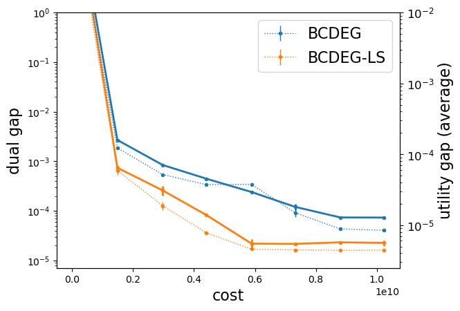
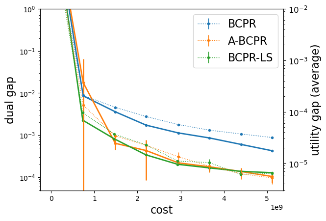
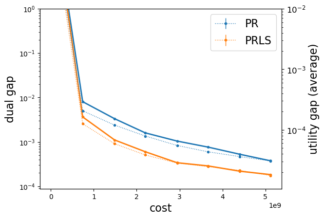
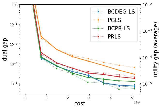
Figure 1: Performance on simulated low-rank instances. Random algorithms were implemented with seeds $0-9$. We also plotted vertical bars representing standard deviations across different seeds. The left y-axis shows performance in terms of the duality gap (solid lines for each algorithm) while the right y-axis shows performance in terms of utilities (dotted line for each algorithm). The x-axis shows units of work performed.

For all markets either BCDEG or BCPR-LS is best on all metrics, followed by PRLS, and PGLS in order. In general, we see that the stochastic block-coordinate algorithms converge faster than their deterministic counterparts across the board, even after thousands of iterations of the deterministic methods. Thus, block-coordinate methods seem to be better even at high precision, while simultaneously achieving better early performance due to the many more updates performed per unit of work.

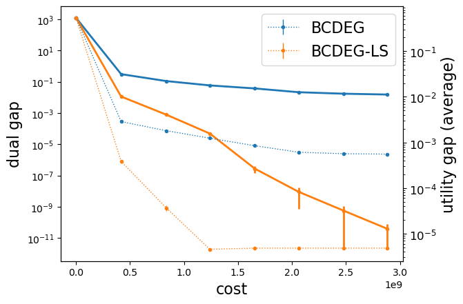
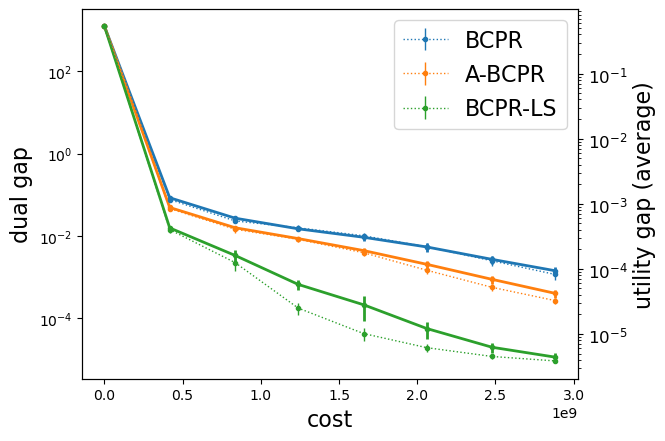
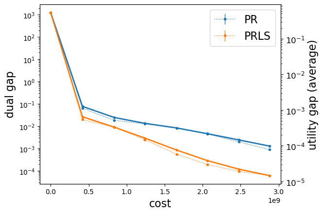
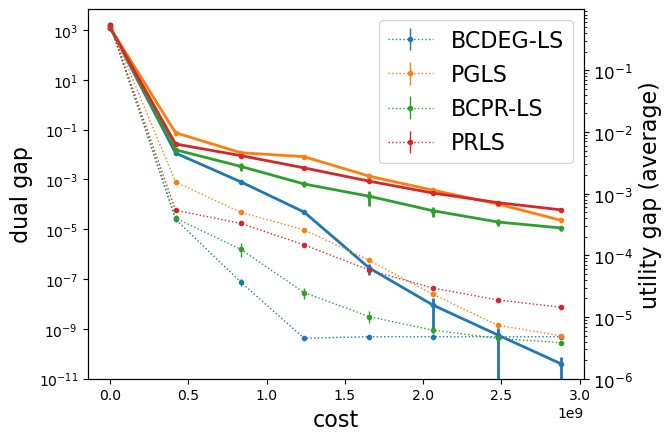
Figure 2: Performance on movierating instances. The plot setup is the same as in Fig. 1.

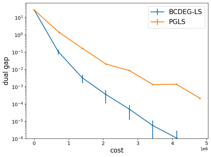
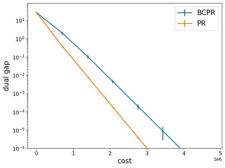
Figure 3: Performance on simulated instances with CES utility with $\rho\in(0,1)$. The setup is the same as in Fig. 1.

CES utilities.

Similar to linear utilities, we generate a $n=m=200$ scale market instance with the CES-utility parameters generated as $v_{ij}=v_{i}v_{j}+\epsilon_{ij}$, where $v_{i}\sim\mathcal{N}(1,0.2^{2})$, $v_{j}\sim\mathcal{N}(1,0.2^{2})$, and $\epsilon_{ij}\sim\emph{uniform}(0,0.2)$. For the CES instances we were not able to obtain high-accuracy solutions from existing conic solvers, and thus we only measure performance in terms of the dual gap. Somewhat surprisingly, we find that for CES utilities vanilla PR converges very fast; faster than BCPR and all versions of BCDEG. Moreover, BCDEG suffers from extremely small stepsizes, so we have to use BCDEG-LS. Here, we used specific small parameters for the distributions in the simulated utilities. More discussion and experiments on CES utilities are given in Appendix E.

9 Conclusion and Future Work

We proposed two stochastic block-coordinate algorithms for computing large-scale ME: (proximal) block-coordinate descent on EG (BCDEG) and block-coordinate proportional response (BCPR). For each algorithm we provided theoretical convergence guarantees and showed numerically that they outperform existing state-of-the-art algorithms. We also provided a new economic interpretation of the projected gradient update used in BCDEG. For future work, we are interested in deriving a sublinear convergence rate for BCPR with adaptive stepsizes, extending it to leverage distributed and parallel computing capabilities, and allowing more general dynamic settings and other buyer utility models.

Appendix A Block Coordinate Descent Algorithm for the EG Program

An efficient implementation of BCDEG

In order to implement Algorithm 1 efficiently, we temporarily store a vector $u\in\mathbb{R}^{n}$ in memory, which represents the current utilities for all buyers. Then, at each iteration $k$, we can dynamically update $u$ by only substituting $x_{\cdot j_{k}}$ while updating a particular block $j_{k}$, which can be done in $O(n)$ time. This avoids performing calculations of the form $u_{i}=\langle v_{i},x_{i}\rangle$, which require $O(nm)$ time when performed for each buyer. See Algorithm 3 for details.

Input: Initial iterate $x^{0}$, stepsizes $\eta_{1}^{k},\eta_{2}^{k},\ldots,\eta_{m}^{k},\;\forall\;k\in\mathbb{N}$

$u_{i}^{0}\leftarrow\langle v_{i},x_{i}^{0}\rangle$ for all $i$;

for $k\leftarrow 1,2,\ldots$ do

       pick $j_{k}\in[m]$ with probability $1/m$;

       for $i\leftarrow 1,2,\cdots,n$ do

             if $u_{i}^{k-1}\geq\underline{u}_{i}$ then

                   $g_{i}^{k-1}\leftarrow-B_{i}\log{u_{i}^{k-1}}$

             else

                   $g_{i}^{k-1}\leftarrow-B_{i}\log{\underline{u}_{i}}-\frac{B_{i}}{\underline{u}_{i}}\left(u_{i}^{k-1}-\underline{u}_{i}\right)+\frac{B_{i}}{2\underline{u}_{i}^{2}}\left(u_{i}^{k-1}-\underline{u}_{i}\right)^{2}$

            

      $x^{k}_{\cdot j_{k}}\leftarrow\text{Prox}(x^{k-1}_{\cdot j_{k}}-\eta_{j_{k}}^{k}g^{k-1})$;

       $x^{k}_{\cdot j}\leftarrow x^{k-1}_{\cdot j}\quad\forall j\neq j_{k}$;

       $u^{k}\leftarrow u^{k-1}+v_{j_{k}}({x^{k}_{\cdot j_{k}}}-{x^{k-1}_{\cdot j_{k}}})$;

      

Algorithm 3 An efficient implementation of BCDEG

(Proximal) Block Coordinate Descent for the EG Program with Line Search

We formally state BCDEG-LS here. This algorithm often outperforms others in our numerical experimental results. The difference to BCDEG is that we check a descent condition (the if condition in Algorithm 4) after performing a tentative proximal step. If the descent condition fails the check (the true case of the if-else statement), then we decrease the stepsize and perform another tentative step. If it passes the check then we commit to the tentative proximal step.

Input: Initial iterate $x^{0}$, initial stepsizes $\eta_{1}^{0},\eta_{2}^{0},\ldots,\eta_{m}^{0}$, $\rho_{-},\rho_{+}\in\mathbb{R}^{+}$

for $k\leftarrow 1,2,\ldots$ do

       pick $j_{k}\in[m]$ with probability $1/m$;

       $g^{k-1}\leftarrow\nabla_{\cdot j_{k}}\tilde{f}(x^{k-1})$;

       $(*)$ $x^{+}_{\cdot j_{k}}\leftarrow\text{Prox}_{\Delta_{n}}\left(x^{k-1}_{\cdot j_{k}}-\eta_{j_{k}}g^{k-1}\right)$;

       $g^{+}\leftarrow\nabla_{\cdot j_{k}}\tilde{f}(x^{+})$;

       if $\eta_{j_{k}}\lVert g^{+}-g^{k-1}\rVert>\lVert x^{+}_{\cdot j_{k}}-x^{k-1}_{\cdot j_{k}}\rVert$ then

             $\eta_{j_{k}}\leftarrow\max\left\{\rho_{-}\eta_{j_{k}},1/L_{j}\right\}$ where $L_{j}$ is computed by (4);

             go back to $(*)$ and re-compute $x^{+}_{\cdot j_{k}}$ and $g^{+}$;

            

       else

             $\eta_{j_{k}}\leftarrow\rho_{+}\eta_{j_{k}}$;

             $x^{k}_{\cdot j_{k}}\leftarrow x^{+}_{\cdot j_{k}}$ and $x^{(k)}_{\cdot j}\leftarrow x^{(k-1)}_{\cdot j}\quad\forall\;j\neq j_{k}$;

            

      

Algorithm 4 BCDEG-LS: (Proximal) Block Coordinate Descent for the EG Program with Line Search

Proof of Eq. 5

Proof.

It can be verified by simple calculations that both $\tilde{f}_{i}(x)$ and $\nabla\tilde{f}_{i}(x)$ are continuous on their domains. Each entry of Hessian matrix of $\tilde{f}$ is of the form:

$$\nabla_{ij}^{2}\tilde{f}(x)=\begin{cases}{B_{i}v_{ij}^{2}}/{u_{i}^{2}(x)}&u_{i}(x)\geq\underline{u}_{i}\\ {B_{i}v_{ij}^{2}}/{\underline{u}_{i}^{2}}&u_{i}(x)<\underline{u}_{i}.\end{cases}$$

Let $x$ and $y$ be two vectors which only differ in one coordinate $j$. Then,

$$\left\lvert\nabla_{ij}\tilde{f}(y)-\nabla_{ij}\tilde{f}(x)\right\rvert=\left\lvert\nabla_{ij}\tilde{f}(y_{i})-\nabla_{ij}\tilde{f}(x_{i})\right\rvert\leq\left\lvert\frac{B_{i}v_{ij}^{2}}{\underline{u}_{i}^{2}}\right\rvert\lvert y_{ij}-x_{ij}\rvert=L_{j}\lVert y_{i}-x_{i}\rVert,$$ (21)

where the inequality is due to

$$\nabla_{ij}^{2}\tilde{f}(x)\leq\frac{B_{i}v_{ij}^{2}}{\underline{u}_{i}^{2}}\leq\max_{i\in[n]}{\frac{B_{i}v_{ij}^{2}}{\underline{u}_{i}^{2}}}=L_{j}.$$

Therefore,

$$\left\lVert\nabla_{\cdot j}\tilde{f}(y)-\nabla_{\cdot j}\tilde{f}(x)\right\rVert^{2}=\sum_{i}\left\lvert\nabla_{ij}\tilde{f}(y)-\nabla_{ij}\tilde{f}(x)\right\rvert^{2}\leq L_{j}^{2}\sum_{i}\lVert y_{i}-x_{i}\rVert^{2}=L_{j}^{2}\lVert y-x\rVert^{2}=L_{j}^{2}\lVert y_{\cdot j}-x_{\cdot j}\rVert^{2},$$ (22)

that is,

$$\left\lVert\nabla_{\cdot j}\tilde{f}(y)-\nabla_{\cdot j}\tilde{f}(x)\right\rVert\leq L_{j}\lVert y_{\cdot j}-x_{\cdot j}\rVert.$$ (23)

To derive (5), we can apply integration:

$$\tilde{f}(y)-\tilde{f}(x)-\langle\nabla_{\cdot j}\tilde{f},y-x\rangle =\int_{0}^{1}\langle\nabla_{\cdot j}\tilde{f}(x+\tau(y-x))-\nabla_{\cdot j}\tilde{f}(x),y-x\rangle\;d\tau$$

$$\leq\int_{0}^{1}\lVert\nabla_{\cdot j}\tilde{f}(x+\tau(y-x))-\nabla_{\cdot j}\tilde{f}(x)\rVert\lVert y-x\rVert\;d\tau$$

$$\leq\int_{0}^{1}\tau L_{j}\lVert y-x\rVert^{2}\;d\tau=\frac{L_{j}}{2}\lVert y-x\rVert^{2}.$$ (24)

∎

Remark.

As a comparison, we provide a proof for a standard (global) Lipschitz constant $L$ as follows. Comparing this with the above proof, we show that when only one block of the variables $x_{\cdot j}$ change, the coordinate-wise Lipschitz constant $L_{j}$ is bounded by the maximum (over all $i$) diagonal value of the Hessian matrix. In contrast, for $L$ it depends on the maximum (over all $i$) sub-trace of the Hessian matrix.

Lemma 5.

For any $j\in[m]$, let

$$L=\max_{i\in[n]}{\frac{B_{i}\lVert v_{i}\rVert^{2}}{\underline{u}_{i}^{2}}}.$$ (25)

Then, for all $x,y\in\mathcal{X}$, we have

$$\tilde{f}(y)\leq\tilde{f}(x)+\langle\nabla\tilde{f}(x),y-x\rangle+\frac{L}{2}{\lVert y-x\rVert^{2}}.$$ (26)

Proof.

Let $x$ and $y$ be two vectors in the domain of $\tilde{f}$, then

$$\left\lvert\nabla_{ij}\tilde{f}(y)-\nabla_{ij}\tilde{f}(x)\right\rvert=\left\lvert\nabla_{ij}\tilde{f}(y_{i})-\nabla_{ij}\tilde{f}(x_{i})\right\rvert\leq\sum_{j^{\prime}=0}^{n-1}\left\lvert\nabla_{ij}\tilde{f}(y^{j^{\prime}}_{i})-\nabla_{ij}\tilde{f}(x^{j^{\prime}}_{i})\right\rvert\leq\sum_{j^{\prime}=0}^{n-1}\left\lvert\frac{\partial^{2}}{\partial x_{ij}\partial x_{ij^{\prime}}}\tilde{f}(x)\right\rvert\left|y_{i}^{j^{\prime}}-x_{i}^{j^{\prime}}\right|$$

where $y^{j^{\prime}}_{i}$ is a vector whose first $(j^{\prime}+1)$’th components are copy of the first $(j^{\prime}+1)$’th components of $y_{i}$ and other components are copy of the last $(m-j^{\prime}-1)$’th components of $x_{i}$; $x^{j^{\prime}}_{i}$ is a vector whose first $j^{\prime}$’th components are copy of the first $j^{\prime}$’th components of $y_{i}$ and other components are copy of the last $(m-j^{\prime})$’th components of $x_{i}$. That is, each pair of $y^{j^{\prime}}_{i}$ and $x^{j^{\prime}}_{i}$ only differ in $(j^{\prime}+1)$’th component. Also, we have $|y_{i}^{j^{\prime}}-x_{i}^{j^{\prime}}|\leq\|y_{i}-x_{i}\|$ for all $i,j^{\prime}$.

$$\sum_{j}\left\lvert\nabla_{ij}\tilde{f}(y)-\nabla_{ij}\tilde{f}(x)\right\rvert^{2}\leq\left(\sum_{j}\left|\nabla_{ij}\tilde{f}(y)-\nabla_{ij}\tilde{f}(x)\right|\right)^{2}\leq\left(\sum_{j}\sum_{j^{\prime}}\frac{B_{i}v_{ij}v_{ij^{\prime}}}{\underline{u}_{i}^{2}}\left\|y_{i}-x_{i}\right\|\right)^{2}\leq L^{2}\left\|y_{i}-x_{i}\right\|^{2}$$

since

$$\frac{\partial^{2}}{\partial x_{ij}\partial x_{ij^{\prime}}}\tilde{f}(x)\leq\frac{B_{i}v_{ij}v_{ij^{\prime}}}{\underline{u}_{i}^{2}}\quad\text{and}\quad\sum_{j}\sum_{j^{\prime}}\frac{B_{i}v_{ij}v_{ij^{\prime}}}{\underline{u}_{i}^{2}}=\frac{B_{i}\lVert v_{i}\rVert^{2}}{\underline{u}_{i}^{2}}\leq\max_{i\in[n]}\frac{B_{i}\lVert v_{i}\rVert^{2}}{\underline{u}_{i}^{2}}=L.$$

Therefore,

$$\left\lVert\nabla\tilde{f}(y)-\nabla\tilde{f}(x)\right\rVert^{2}=\sum_{i}\sum_{j}\left\lvert\nabla_{ij}\tilde{f}(y)-\nabla_{ij}\tilde{f}(x)\right\rvert^{2}\leq L^{2}\sum_{i}\lVert y_{i}-x_{i}\rVert^{2}=L^{2}\lVert y-x\rVert^{2}.$$ (27)

∎

Note that this is a tighter bound than Gao and Kroer (2020) because $\max_{i\in[n]}\frac{B_{i}\lVert v_{i}\rVert^{2}}{\underline{u}_{i}^{2}}\leq\max_{i\in[n]}\frac{B_{i}}{\underline{u}_{i}^{2}}\max_{i\in[n]}\lVert v_{i}\rVert^{2}$.

Proof of Lemma 2

Proof.

Since $g(u)$ is strongly convex, there exists a unique $u^{*}$ such that

$$g(u^{*})=g^{*}\quad\quad Ax^{*}=u^{*}\quad\forall x^{*}\in\mathcal{X}^{*}.$$

Thus, the set of optimal solutions $\mathcal{X}^{*}$ can be described by the following polyhedral set for some $C$:

$$\mathcal{X}^{*}=\{x^{*}:Ax^{*}=u^{*},Cx^{*}\leq d\}.$$

Assume that the optimal polyhedral set $\mathcal{X}^{*}$ is non-empty, then the Hoffman inequality (Hoffman 2003) tells us there exists some positive constant such that

$$\lVert x-x^{*}\rVert\leq\theta(A,C)\begin{Vmatrix}\begin{bmatrix}Ax-u^{*}\\ \left(Cx-d\right)^{+}\end{bmatrix}\end{Vmatrix}\quad\forall\;x.$$ (28)

Let $\mathcal{X}$ be the set of feasible allocations. For any $x\in\mathcal{X}$ such that $Cx\leq d$, we have

$$\lVert x-x^{*}\rVert\leq\theta(A,C)\lVert Ax-Ax^{*}\rVert.$$ (29)

From strong convexity of $\tilde{g}$ and (29), we have

$$F^{*}=F(x^{*}) \geq F(x)+\langle\nabla\tilde{f}(x),x^{*}-x\rangle+\frac{\mu}{2}\lVert Ax^{*}-Ax\rVert^{2}+\psi(x^{*})-\psi(x)$$

$$\geq F(x)+\langle\nabla\tilde{f}(x),x^{*}-x\rangle+\frac{\mu}{2\theta^{2}(A,C)}\lVert x^{*}-x\rVert^{2}+\psi(x^{*})-\psi(x).$$ (30)

If $L\geq\frac{\mu}{\theta^{2}(A,C)}$, then

$$F^{*} \geq F(x)+\langle\nabla\tilde{f}(x),x^{*}-x\rangle+\frac{\mu}{2\theta^{2}(A,C)}\lVert x^{*}-x\rVert^{2}+\psi(x^{*})-\psi(x)$$

$$\geq F(x)+\min_{y\in\mathbb{R}^{nm}}\left\{\langle\nabla\tilde{f}(x),y-x\rangle+\frac{\mu}{2\theta^{2}(A,C)}{\lVert y-x\rVert}^{2}+\psi(y)-\psi(x)\right\}$$

$$=F(x)-\frac{\theta^{2}(A,C)}{2\mu}\mathcal{D}_{\psi}(x,\frac{\mu}{\theta^{2}(A,C)}).$$ (31)

Hence,

$$\frac{1}{2}\mathcal{D}_{\psi}(x,\frac{\mu}{\theta^{2}(A,C)})\geq\frac{\mu}{\theta^{2}(A,C)}(F(x)-F^{*}).$$ (32)

Since $\mathcal{D}(x,\cdot)$ is non-decreasing (Karimi, Nutini, and Schmidt 2016, Lemma 1), we have

$$\frac{1}{2}\mathcal{D}_{\psi}(x,L)\geq\frac{\mu}{\theta^{2}(A,C)}(F(x)-F^{*}).$$ (33)

If $L<\frac{\mu}{\theta^{2}(A,C)}$, then

$$F^{*} \geq F(x)+\langle\nabla\tilde{f}(x),x^{*}-x\rangle+\frac{\mu}{2\theta^{2}(A,C)}\lVert x^{*}-x\rVert^{2}+\psi(x^{*})-\psi(x)$$

$$\geq F(x)+\langle\nabla\tilde{f}(x),x^{*}-x\rangle+\frac{L}{2}\lVert x^{*}-x\rVert^{2}+\psi(x^{*})-\psi(x)$$

$$\geq F(x)+\min_{y\in\mathbb{R}^{nm}}\left\{\langle\nabla\tilde{f}(x),y-x\rangle+\frac{L}{2}{\lVert y-x\rVert}^{2}+\psi(y)-\psi(x)\right\}$$

$$=F(x)-\frac{1}{2L}\mathcal{D}_{\psi}(x,L).$$ (34)

Hence,

$$\frac{1}{2}\mathcal{D}_{\psi}(x,L)\geq L(F(x)-F^{*}).$$ (35)

Combining the two cases, we can conclude (6). ∎

Proof of Theorem 1

The following convergence analysis is typical for uniform (block) coordinate descent algorithms. Leveraging (6), it is easy to derive a linear convergence rate for both BCDEG and BCDEG-LS. This proof scheme was given in Karimi, Nutini, and Schmidt (2016, Appendix H), but here we give a variant with different stepsizes across blocks and iterations.

Proof.

To remind readers of notations, we define (again)

$$T_{j}(x)=\arg\min_{y_{\cdot j}}\langle\nabla_{\cdot j}f(x),y_{\cdot j}-x_{\cdot j}\rangle+L_{j}\lVert y_{\cdot j}-x_{\cdot j}\rVert^{2}+\psi_{j}(y_{\cdot j})$$ (36)

for BCDEG and

$$T_{j}^{k}(x)=\arg\min_{y_{\cdot j}}\langle\nabla_{\cdot j}f(x),y_{\cdot j}-x_{\cdot j}\rangle+\frac{1}{\eta_{j}^{k}}\lVert y_{\cdot j}-x_{\cdot j}\rVert^{2}+\psi_{j}(y_{\cdot j})$$ (37)

for BCDEG-LS.

Then, we have (e.g. for BCDEG)

$$\mathbf{E}[F(x^{k+1})\nonscript\;|\nonscript\;x^{k}] \leq F(x^{k})+\frac{1}{m}\sum_{j}\left\{\langle\nabla_{\cdot j}\tilde{f}(x^{k}),T_{j}(x)-x_{\cdot j}^{k}\rangle+\frac{L_{j}}{2}\lVert T_{j}(x)-x_{\cdot j}^{k}\rVert^{2}+\psi_{j}(T_{j}(x))\right\}$$ (38)

$$=\tilde{f}(x^{k})+\frac{1}{m}\sum_{j}\min_{y_{\cdot j}}\left\{\langle\nabla_{\cdot j}\tilde{f}(x^{k}),y_{\cdot j}-x_{\cdot j}^{k}\rangle+\frac{L_{j}}{2}\lVert y_{\cdot j}-x_{\cdot j}^{k}\rVert^{2}+\psi_{j}(y_{\cdot j})\right\}$$

$$=\tilde{f}(x^{k})+\frac{1}{m}\min_{y}\left\{\langle\nabla\tilde{f}(x^{k}),y-x^{k}\rangle+\frac{1}{2}{\lVert y-x^{k}\rVert}_{L}^{2}+\psi(y)\right\}$$

$$=F(x^{k})+\frac{1}{m}\min_{y}\left\{\langle\nabla\tilde{f}(x^{k}),y-x^{k}\rangle+\frac{1}{2}{\lVert y-x^{k}\rVert}_{L}^{2}+\psi(y)-\psi(x^{k})\right\}$$

$$\leq F(x^{k})+\frac{1}{m}\min_{y}\left\{\langle\nabla\tilde{f}(x^{k}),y-x^{k}\rangle+\frac{L_{\max}}{2}\lVert y-x^{k}\rVert^{2}+\psi(y)-\psi(x^{k})\right\}$$

$$=F(x^{k})-\frac{1}{2mL_{\max}}\mathcal{D}_{\psi}(x^{k},L_{\max}),$$ (39)

where we used Lipschitz smoothness (or line search condition for BCDEG-LS) of $\tilde{f}$, the definition of $T_{j}(x)$, and separability on each block $j$.

For BCDEG-LS, replacing (38) with the following inequality:

$$\mathbf{E}[F(x^{k+1})\nonscript\;|\nonscript\;x^{k}]\leq F(x^{k})+\frac{1}{m}\sum_{j}\left\{\langle\nabla_{\cdot j}\tilde{f}(x^{k}),T_{j}(x)-x_{\cdot j}^{k}\rangle+\frac{1}{2\eta_{j}^{k}}\lVert T_{j}(x)-x_{\cdot j}^{k}\rVert^{2}+\psi_{j}(T_{j}(x))\right\},$$ (40)

and by $1/\eta_{j}^{k}\leq L_{j}\leq L_{\max}$ (used in the last inequality) we have (39).

By Lemma 2, we have

$$\mathbf{E}[F(x^{k+1})\nonscript\;|\nonscript\;x^{k}]-F(x^{k})\leq-\frac{1}{2mL_{\max}}\mathcal{D}_{\psi}(x^{k},L_{\max})\leq-\min\left\{\frac{\mu}{mL_{\max}\theta^{2}(A,C)},\frac{1}{m}\right\}(F(x^{k})-F^{*}).$$ (41)

Subtracting $F^{*}$ on the both sides, Rearranging the above inequality, and taking expectation w.r.t. $j_{1},\ldots,j_{k}$, we obtain (7) by induction. ∎

Appendix B Algorithm Details for Projection onto a Simplex

We show a key theorem for projection onto a simplex algorithm and a formally stated algorithm as background for readers who are not familiar with this algorithm.

Theorem 6.

(Chen and Ye 2011, Theorem 2.2.) For any vector $y\in\mathbb{R}^{n}$, the projection of $y$ onto $\Delta^{n}$ is obtained by the positive part of $y-\hat{t}$:

$$x=(y-\hat{t})^{+},$$ (42)

where $\hat{t}$ is the only one in $\{t_{i}:i=0,\ldots,n-1\}$ that falls into the corresponding interval as follows,

$$t_{i}:=\frac{\sum_{j=i+1}^{n}{y_{(j)}-1}}{n-i},i=0,\ldots,n-1,\quad\text{ where }t_{1}\leq y_{(1)}\text{ and }y_{(i)}\leq t_{i}\leq y_{(i+1)},i=1,\ldots,n-1.$$ (43)

Hence, to find $x$, we only need to find the $t_{i}$ in (43) that falls into the corresponding interval, claim it as the optimal $\hat{t}$, and then compute $x$ based on (42). The following algorithm is implied by the above theorem.

Input: $y=(y_{1},y_{2},\ldots,y_{n})^{\top}\in\mathbb{R}^{n}$

Output: $x=(x_{1},x_{2},\ldots,x_{n})^{\top}\in\mathbb{R}^{n}$ as the projection of $y$ onto $\Delta^{n}$

Sort $y$ in the ascending order as $y_{(1)}\leq\cdots\leq y_{(n)}$;

$\hat{t}\leftarrow\frac{\sum_{j=1}^{n}{y_{(j)}}-1}{n}$;

for $i\leftarrow n-1,\ldots,1$ do

       $t_{i}\leftarrow\frac{\sum_{j=i+1}^{n}{y_{(j)}}-1}{n-i}$;

       if $t_{i}\geq y_{(i)}$ then

             $\hat{t}\leftarrow t_{i}$ and break the loop;

            

      

$x\leftarrow(y-\hat{t})^{+}$;

Algorithm 5 Projection onto a Simplex

Discussion on alternative algorithms for projection onto a simplex

In this paper, we assume that the above algorithm is an efficient method to project an array onto a simplex, and interpret projection-type ME-solving algorithms based on this algorithm. There are several variants of this type of projection algorithm, and some of them give improved complexity results or practical performance. Condat (2016) summarize most of these algorithms, which use different methods to find the correct threshold value. Some of these algorithms exploit problem structure to obtain $O(n)$ expected or practical complexity. However, in the worst case, there is still no better result than $O(n\log(n))$. Perez et al. (2020) proposed a method with a worst-case linear-time complexity result. Their result is analogous to bucket sort, it assumes that the set of possible values that you might encounter is constant.

Appendix C Block Coordinate Proportional Response

Block Coordinate Proportional Response with Line Search

We formally state Block Coordinate Proportional Response with Line Search (BCPR-LS) algorithm as follows. Note that $\delta\in[0,1)$ is a “conservative” factor - we can set $\delta>0$ to use more conservative stepsize strategy than standard line search ($\delta=0$). In $\delta>0$ case, we can guarantee some (weak) convergence property for BCPR-LS.

Input: $b^{0}\in\mathbb{R}^{n\times m},p^{0}\in\mathbb{R}^{m},\alpha_{1},\ldots,\alpha_{n}\in\mathbb{R}^{+},\rho_{-},\rho_{+}\in\mathbb{R}^{+}$

for $k\leftarrow 1,2,\ldots$ do

       pick $i_{k}\in[n]$ with probability $1/n$;

       (*) compute $b_{i_{k}}^{+}$ based on (14) with stepsize $(1-\delta)\alpha_{i_{k}}$;

       $p^{+}\leftarrow p+b_{i_{k}}^{+}-b_{i_{k}}$;

       if $\alpha_{i_{k}}D_{\rm KL}(p^{+},p)>D_{\rm KL}(b_{i_{k}}^{+},b_{i_{k}})$ then

             $\alpha_{i_{k}}\leftarrow\rho_{-}\alpha_{i_{k}}$;

             go back to (*) and re-compute $b_{ik}^{+}$ and $p^{+}$;

            

       else

             $\alpha_{i_{k}}\leftarrow\rho_{+}\alpha_{i_{k}}$;

             $b_{i_{k}}^{k}\leftarrow b_{i_{k}}^{+}$ and $b_{i^{\prime}}^{k}\leftarrow b_{i^{\prime}}^{k-1}\quad\forall\;i^{\prime}\neq i_{k}$;

            

      

Algorithm 6 Block Coordinate Proportional Response (BCPR) with Line Search

Proof of Eq. 14

Proof.

The original minimization problem can be solved by Lagrangian method by introducing a Lagrangian multiplier $\lambda$:

$$\min\mathcal{L}(a_{1},a_{2},\ldots,a_{m},\lambda)={\langle\nabla_{i}\varphi(b),a-b_{i}\rangle+\frac{1}{\alpha}D_{\text{KL}}(a,b_{i})+\lambda\Big{(}B_{i}-\sum_{j}{a_{j}}\Big{)}}.$$ (44)

Let $\nabla_{a_{1},a_{2},\ldots,a_{m},\lambda}\mathcal{L}=0$, we have

$$\frac{\partial}{\partial a_{j}}\bigg{(}\langle\nabla_{i}\varphi(b),a-b_{i}\rangle+\frac{1}{\alpha}D_{\rm KL}(a,b_{i})\bigg{)}=\lambda\quad\forall j=1,2,\ldots,m\quad\mbox{and}\quad\sum_{j}{a_{j}}=B_{i}.$$ (45)

The partial derivatives are equal to

$$1-\log{\left(\frac{v_{ij}}{p_{j}}\right)}+\frac{1}{\alpha}\left(1+\log{\frac{a_{j}}{b_{ij}}}\right)\quad\forall j=1,2,\ldots,m.$$

Let $a_{j}=\frac{1}{Z}b_{ij}\Big{(}\frac{v_{ij}}{p_{j}}\Big{)}^{\alpha}$, $\lambda=1+\frac{1}{\alpha}-\log{Z}$, where $Z=\frac{1}{B_{i}}\sum_{j}{b_{ij}\Big{(}\frac{v_{ij}}{p_{j}}\Big{)}^{\alpha}}$. We can verify that

$$1+\frac{1}{\alpha}-\log{Z}=\frac{\partial}{\partial a_{j}}\left(\langle\nabla_{i}\varphi(b),a-b_{i}\rangle+\frac{1}{\alpha}D_{\rm KL}(a,b_{i})\right)=\lambda\quad\mbox{and}\quad\sum_{j}{a_{j}}=\frac{1}{Z}\sum_{j}{b_{ij}\left(\frac{v_{ij}}{p_{j}}\right)^{\alpha}}=B_{i}.$$ (46)

Therefore, $(a_{1},a_{2},\ldots,a_{m},\lambda)$ is a stationary point of the Lagrange function. $a=(a_{1},a_{2},\ldots,a_{m})$ is a solution to the original minimization problem due to the convexity of the problem. ∎

Coordinate-wise relative smoothness (in expectation)

In the rest of this section, except for A-BCPR, we use general Bregman distance $D(a,b)$ between $a,b\in\mathbb{R}^{n}$ and $D_{L}(a,b)=\sum_{i}L_{i}D_{i}(a_{i},b_{i})$ where $D_{i}(a_{i},b_{i})$ is coordinate-wise Bregman distance and $L\in\mathbb{R}^{n}$. We also introduce $T^{k}=\sum_{i}T_{i}^{k}$ as below (similar to $l_{2}$ norm block coordinate descent):

$$T^{k}=\sum_{i}{T_{i}^{k}}=\operatorname*{arg\,min}_{a\in\mathbb{R}^{n\times m}}\left\{\langle\nabla\varphi(b),a-b\rangle+\sum_{i}\frac{1}{\alpha_{i}^{k}}D_{i}(a_{i},b_{i})+r(a)\right\}.$$ (47)

Then, it is standard to have the following lemma.

Lemma 6.

If $b^{k}$ is the random iterates generated by Algorithm 6, then

$$\mathbf{E}\left[\varphi(b^{k+1})\nonscript\;\middle|\nonscript\;b^{k}\right]\leq \varphi(b^{k})+\frac{1}{n}\langle\nabla\varphi(b^{k}),T^{k}-b^{k}\rangle+\frac{1}{n}D_{1/\alpha^{k}}(T^{k},b^{k})$$ (48)

$$= \varphi(b^{k})+\mathbf{E}\left[\langle\nabla\varphi(b^{k}),b^{k+1}-b^{k}\rangle\nonscript\;|\nonscript\;b^{k}\right]+\mathbf{E}\left[D_{1/\alpha^{k}}(b^{k+1},b^{k})\nonscript\;\middle|\nonscript\;b^{k}\right].$$ (49)

Note that (48) is a special case (the cardinality of sampling equals to $1$, uniform sampling) of $h$-ESO assumption defined in Hanzely and Richtárik (2021). Essentially, this is coordinate-wise relative smoothness in expectation.

Proof.

Given any coordinate $i$, we have (let $b^{+}$ and $p^{+}$ be the next iterates of $b$ and $p$, respectively)

$$\varphi(b^{+})-\varphi(b)-\langle\nabla_{i}{\varphi(b)},b_{i}^{+}-b_{i}\rangle= \varphi(b^{+})-\varphi(b)-\langle\nabla{\varphi(b)},b^{+}-b\rangle$$

$$= -\sum_{i,j}{b_{ij}^{+}\log{\frac{v_{ij}}{p_{j}^{+}}}}+\sum_{i,j}{b_{ij}\log{\frac{v_{ij}}{p_{j}}}}-\sum_{i,j}{\big{(}1-\log{\frac{v_{ij}}{p_{j}}}\big{)}(b_{ij}^{+}-b_{ij})}$$

$$= \sum_{i,j}{b_{ij}^{+}\log{\frac{p_{j}^{+}}{p_{j}}}}=\sum_{j}{p_{j}^{+}\log{\frac{p_{j}^{+}}{p_{j}}}},$$ (50)

and $D_{\rm KL}(b_{i}^{+},b_{i})=\sum_{j}{b_{ij}^{+}\log{\frac{b_{ij}^{+}}{b_{ij}}}}$. The line search condition ensures

$$\varphi(b^{+})\leq\varphi(b)+\langle\nabla_{i}{\varphi(b)},b_{i}^{+}-b_{i}\rangle+\frac{1}{\alpha_{i}}D_{\text{KL}}(b_{i}^{+},b_{i}).$$ (51)

Note that if we let $a\in\mathbb{R}$ and $f(x)=x\log{\frac{x}{x-a}}$, then $f^{\prime}(x)=\log{(1+\frac{a}{x-a})}-\frac{a}{x-a}\leq\frac{a}{x-a}-\frac{a}{x-a}=0$. Since $p_{j}^{+}-p_{j}=b_{ij}^{+}-b_{ij}$, let $a=b_{ij}^{+}-b_{ij}$, we have

$$\sum_{j}{p_{j}^{+}\log{\frac{p_{j}^{+}}{p_{j}}}}=\sum_{j}f(p_{j}^{+})\leq\sum_{j}f(b_{ij}^{+})=\sum_{j}{b_{ij}^{+}\log{\frac{b_{ij}^{+}}{b_{ij}}}},$$ (52)

where we use $p_{j}^{+}\geq b_{ij}^{+}$ and monotonity of $f(x)$. Note that (51) always holds when $\alpha_{i}=1$ for all $i$.

Hence, by separability on each block of coordinates we have

$$\mathbf{E}\left[\varphi(b^{k+1})\nonscript\;\middle|\nonscript\;b^{k}\right]\leq \sum_{i}\frac{1}{n}\left\{\varphi(b^{k})+\langle\nabla_{i}{\varphi(b)},T_{i}^{k}-b_{i}^{k}\rangle+\frac{1}{\alpha_{i}^{k}}D_{\rm KL}(T_{i}^{k},b_{i}^{k})\right\}$$

$$= \varphi(b^{k})+\frac{1}{n}\langle\nabla\varphi(b^{k}),T^{k}-b^{k}\rangle+\frac{1}{n}D_{1/\alpha^{k}}(T^{k},b^{k}).$$ (53)

As we know

$$\mathbf{E}\left[\langle\nabla\varphi(b^{k}),b^{k+1}-b^{k}\rangle\nonscript\;|\nonscript\;b^{k}\right]=\sum_{i}\frac{1}{n}\langle\nabla_{i}\varphi(b^{k}),T_{i}^{k}-b_{i}^{k}\rangle=\frac{1}{n}\langle\nabla\varphi(b^{k}),T^{k}-b^{k}\rangle$$ (54)

and

$$\mathbf{E}\left[D_{1/\alpha^{k}}(b^{k+1},b^{k})\nonscript\;\middle|\nonscript\;b^{k}\right]=\sum_{i}\frac{1}{n}\frac{1}{\alpha_{i}^{k}}D_{i}(T_{i}^{k},b_{i}^{k})=\frac{1}{n}D_{1/\alpha^{k}}(T^{k},b^{k}),$$ (55)

(48) and (49) are equivalent.

∎

A useful descent lemma

Next, we will consider BCPR with line search (BCPR-LS). We can directly see that BCPR (with fixed stepsizes)’s sublinear convergence rate is a special case of our convergence property.

The following lemma can be derived from Lemma 6 and three point property (e.g. Hanzely and Richtárik (2021, Lemma 3.5)). Beyond existing results, we prove a version for line search and $\alpha_{i}^{k}=(1-\delta)/L_{i}^{k}$ stepsize strategy.

Lemma 7.

If $b^{k}$ is the random iterates generated by Algorithm 6, then

$$\mathbf{E}\left[\Phi(b^{k+1})\nonscript\;\middle|\nonscript\;b^{k}\right] \leq\frac{n-1}{n}\Phi(b^{k})+\frac{1}{n}\Big{\{}\Phi(u)+D_{\alpha^{k}}(u,b^{k})-D_{\alpha^{k}}(u,T^{k})-\delta D_{\alpha^{k}}(T^{k},b^{k})\Big{\}}$$

$$=\frac{n-1}{n}\Phi(b^{k})+\frac{1}{n}\Phi(u)+\frac{1}{n}D_{\frac{1}{\alpha^{k}}}(u,b^{k})-\frac{1}{n}\mathbf{E}\left[D_{\frac{1}{\alpha^{k}}}(u,b^{k+1})\nonscript\;\middle|\nonscript\;b^{k}\right]-\frac{\delta}{n}\mathbf{E}\left[D_{\frac{1}{\alpha^{k}}}(b^{k+1},b^{k})\nonscript\;\middle|\nonscript\;b^{k}\right],$$ (56)

where $T^{k}$ defined in (47) and $u\in{\rm dom}\,\varphi\cup{\rm dom}\,h$.

Proof.

Given any $b^{k}$ (iterate at the $k$th iteration), we have

$$\mathbf{E}\left[\Phi(b^{k+1})\nonscript\;\middle|\nonscript\;b^{k}\right]\leq \varphi(b^{k})+\mathbf{E}\left[\langle\nabla\varphi(b^{k}),b^{k+1}-b^{k}\rangle\nonscript\;|\nonscript\;b^{k}\right]+\mathbf{E}\left[D_{L^{k}}(b^{k+1},b^{k})\nonscript\;\middle|\nonscript\;b^{k}\right]+\mathbf{E}\left[r(b^{k+1})\nonscript\;\middle|\nonscript\;b^{k}\right]$$

$$= \varphi(b^{k})+\frac{1}{n}\langle\nabla\varphi(b^{k}),T^{k}-b^{k}\rangle+\frac{1}{n}D_{L^{k}}(T^{k},b^{k})+\frac{1}{n}\sum_{i}r_{i}\left(T_{i}^{k}\right)+\frac{1}{n}\sum_{i}\sum_{i^{\prime}\neq i}r_{i^{\prime}}\left(b_{i^{\prime}}^{k}\right)$$

$$= \varphi(b^{k})+\frac{1}{n}\langle\nabla\varphi(b^{k}),T^{k}-b^{k}\rangle+\frac{1}{n}D_{L^{k}}(T^{k},b^{k})+\frac{1}{n}r\left(T^{k}\right)+\frac{n-1}{n}r\left(b^{k}\right)$$

$$= \frac{n-1}{n}\Phi(b^{k})+\frac{1}{n}\left\{\varphi(b^{k})+\langle\nabla\varphi(b^{k}),T^{k}-b^{k}\rangle+D_{L^{k}}(T^{k},b^{k})+r\left(T^{k}\right)\right\},$$ (57)

which follows from Lemma 6 and separability of $r$.

By the optimality of (47), we have

$$v^{k}=-\nabla\varphi(b^{k})-\sum_{i}\frac{1}{\alpha_{i}^{k}}\nabla h_{i}(T_{i}^{k})+\sum_{i}\frac{1}{\alpha_{i}^{k}}\nabla h_{i}(b^{k}_{i})$$ (58)

for some $v^{k}\in\partial r(T^{k})$.

By convexity of $\varphi$ and $r$, for any $u\in{\rm dom}\,\varphi\cup{\rm dom}\,h$,

$$r(T^{k})\leq r(u)-\langle v^{k},u-T^{k}\rangle,$$ (59)

$$\varphi(b^{k})\leq\varphi(u)-\langle\nabla\varphi(b^{k}),u-b^{k}\rangle.$$ (60)

By the definition of Bregman distance we have so-called three point identity:

$$\langle\nabla h_{i}(T_{i}^{k})-\nabla h_{i}(b^{k}_{i}),u_{i}-T_{i}^{k}\rangle=D_{i}(u_{i},b^{k}_{i})-D_{i}(u_{i},T_{i}^{k})-D_{i}(T_{i}^{k},b^{k}_{i})$$ (61)

for all $u_{i}\in{\rm dom}\,h_{i}$ and all $i\in[n]$.

Then, by combining all above inequalities and equalities we have

$$\mathbf{E}\left[\Phi(b^{k+1})\nonscript\;\middle|\nonscript\;b^{k}\right]\leq \frac{n-1}{n}\Phi(b^{k})+\frac{1}{n}\left\{\varphi(b^{k})+\langle\nabla\varphi(b^{k}),T^{k}-b^{k}\rangle+D_{L^{k}}(T^{k},b^{k})+r\left(T^{k}\right)\right\}$$

$$\leq \frac{n-1}{n}\Phi(b^{k})+\frac{1}{n}\left\{\varphi(b^{k})+\langle\nabla\varphi(b^{k}),u-b^{k}\rangle\right\}$$

$$\quad+\frac{1}{n}\left\{D_{L^{k}}(T^{k},b^{k})+r\left(u\right)+\sum_{i}\frac{1}{\alpha_{i}^{k}}\langle\left(\nabla h_{i}\left(T_{i}^{k}\right)-\nabla h_{i}\left(b_{i}^{k}\right)\right),u-T^{k}\rangle\right\}$$

$$\leq \frac{n-1}{n}\Phi(b^{k})+\frac{1}{n}\varphi(u)+\frac{1}{n}\left\{D_{L^{k}}(T^{k},b^{k})+r\left(u\right)+\sum_{i}\frac{1}{\alpha_{i}^{k}}\langle\left(\nabla h_{i}\left(T_{i}^{k}\right)-\nabla h_{i}\left(b_{i}^{k}\right)\right),u-T^{k}\rangle\right\}$$

$$= \frac{n-1}{n}\Phi(b^{k})+\frac{1}{n}\left\{\Phi(u)+D_{\alpha^{k}}(u,b^{k})-D_{\alpha^{k}}(u,T^{k})-\delta D_{\alpha^{k}}(T^{k},b^{k})\right\}$$ (62)

for any $u$. Here, we use (57), (59) with (58), (60), (61) and $\alpha_{i}^{k}=(1-\delta)/L_{i}^{k}$ for $\delta\in[0,1)$. (56) follows from identity relations similar to (54) and (55). ∎

The following corollaries provide some (weak) convergence properties for BCPR-LS.

Corollary 1.

If $b^{k}$ is the random iterates generated by Algorithm 6, then

1. $\mathbf{E}[\Phi(b^{k})]$ is non-increasing;

2. $\sum_{k=0}^{\infty}\mathbf{E}[D_{1/\alpha^{k}}(b^{k+1},b^{k})]<\infty$, $\mathbf{E}[D_{i}(b_{i}^{k+1},b_{i}^{k})]\rightarrow 0$ as $k\rightarrow\infty$ for all $i$;

3. $\sum_{k=0}^{\infty}\mathbf{E}[D_{1/\alpha^{k}}(b^{k},b^{k+1})]<\infty$, $\mathbf{E}[D_{i}(b_{i}^{k},b_{i}^{k+1})]\rightarrow 0$ as $k\rightarrow\infty$ for all $i$;

4. $\mathbf{E}[D_{1/\alpha^{k}}(b^{*},b^{k})]\leq\mathbf{E}[D_{1/\alpha^{k}}(b^{*},b^{k+1})]$ as $k\rightarrow\infty$.

Proof.

Let $u=b^{k}$ in (56), we have

$$\mathbf{E}\left[\Phi(b^{k+1})\nonscript\;\middle|\nonscript\;b^{k}\right]\leq\Phi(b^{k})$$ (63)

by using non-negativity of Bregman distance. This shows objective descent in expectation.

Also, we have

$$\mathbf{E}[\Phi(b^{k+1})|b^{k}]\leq\Phi(b^{k})+\frac{1}{n}\left\{-D_{\alpha^{k}}(b^{k},T^{k})-\delta D_{\alpha^{k}}(T^{k},b^{k})\right\}\leq\Phi(b^{k})-\frac{\delta}{n}D_{\alpha^{k}}(T^{k},b^{k}).$$ (64)

As we know $\mathbf{E}[D_{\alpha^{k}}(b^{k+1},b^{k})|b^{k}]=\frac{1}{n}D_{\alpha^{k}}(T^{k},b^{k})$, (64) is equivalent to

$$\delta\mathbf{E}[D_{\alpha^{k}}(b^{k+1},b^{k})|b^{k}]\leq\Phi(b^{k})-\mathbf{E}[\Phi(b^{k+1})|b^{k}].$$ (65)

Summing up (65) over $0,1,\ldots,k-1$ and taking expectation w.r.t. $i_{0},i_{1},\ldots,i_{k-1}$, we have

$$\delta\sum_{l=0}^{k}\mathbf{E}[D_{\alpha^{l}}(b^{l+1},b^{l})]\leq\Phi(b^{0})-\mathbf{E}[\Phi(b^{k})]<\infty.$$ (66)

Let $k\rightarrow\infty$, we have $\sum_{l=0}^{\infty}\mathbf{E}[D_{\alpha^{l}}(b^{l+1},b^{l})]<\infty$, which implies $\mathbf{E}[D_{\alpha^{k}}(b^{k+1},b^{k})]\rightarrow 0$ as $k\rightarrow\infty$.

Similar to (64), we have

$$\mathbf{E}[\Phi(b^{k+1})|b^{k}]\leq\Phi(b^{k})+\frac{1}{n}\left\{-D_{\alpha^{k}}(b^{k},T^{k})-\delta D_{\alpha^{k}}(T^{k},b^{k})\right\}\leq\Phi(b^{k})-\frac{1}{n}D_{\alpha^{k}}(b^{k},T^{k}).$$ (67)

Then, (iii) follows from the same argument as the proof of (ii).

Because $\mathbf{E}[\Phi(b^{k})]$ is non-increasing and $\mathbf{E}[\Phi(b^{k})]\geq\Phi^{*}>-\infty$, $\mathbf{E}[\Phi(b^{k+1})-\Phi(b^{k})]\rightarrow 0$.

Let $u=b^{*}$ in (62), we have

$$\mathbf{E}\left[\Phi(b^{k+1})\nonscript\;\middle|\nonscript\;b^{k}\right]\leq\frac{n-1}{n}\Phi(b^{k})+\frac{1}{n}\left\{\Phi(b^{*})+D_{\alpha^{k}}(b^{*},b^{k})-D_{\alpha^{k}}(b^{*},T^{k})\right\}$$ (68)

due to the non-negativity of Bregman distance. Rearranging (68), summing it up over $0,\ldots,k$ and using the tower property, we have

$$(n-1)\mathbf{E}[\Phi(b^{k+1})-\Phi(b^{k})]+\left(\mathbf{E}[\Phi(b^{k+1})]-\Phi(u)\right)\leq\mathbf{E}[D_{\alpha^{k}}(u,b^{k})]-\mathbf{E}[D_{\alpha^{k}}(u,b^{k+1})].$$ (69)

When $k\rightarrow\infty$, the left hand side of (69) goes to be non-negative, which imples (iv). ∎

Proof of Theorem 2

Proof.

For any $u\in{\rm dom}\,h$, we have

$$\mathbf{E}\left[D_{1/\alpha^{k}}(u,b^{k+1})\nonscript\;\middle|\nonscript\;b^{k}\right] =\sum_{i}\frac{1}{n}\left\{\frac{1}{\alpha_{i}^{k}}D_{i}(u_{i},T_{i}^{k})+\sum_{i^{\prime}\neq i}\frac{1}{\alpha_{i^{\prime}}^{k}}D_{i}(u_{i^{\prime}},b_{i^{\prime}}^{k})\right\}$$

$$=\frac{1}{n}D_{1/\alpha^{k}}(u,T^{k})+\frac{n-1}{n}D_{1/\alpha^{k}}(u,b^{k}).$$ (70)

By Lemma 7 and (70), let $u=b^{*}$, then we get

$$\mathbf{E}\left[\Phi(b^{k+1})+D_{1/\alpha^{k}}(b^{*},b^{k+1})\nonscript\;\middle|\nonscript\;b^{k}\right]\leq\frac{n-1}{n}\Phi(b^{k})+\frac{1}{n}\Phi(b^{*})+D_{1/\alpha^{k}}(b^{*},b^{k}).$$ (71)

Rearranging (71), we attain

$$\mathbf{E}\left[\Phi(b^{k+1})-\Phi(b^{*})+D_{1/\alpha^{k}}(b^{*},b^{k+1})\nonscript\;\middle|\nonscript\;b^{k}\right]\leq\frac{n-1}{n}\left(\Phi(b^{k})-\Phi(b^{*})\right)+D_{1/\alpha^{k}}(b^{*},b^{k}).$$ (72)

We take the expectation of (72) with respect to $\{i_{0},i_{1},\ldots,i_{k}\}$ and sum this inequality over $l=0,\ldots,k$ to obtain

$$\mathbf{E}\left[\Phi(b^{k+1})-\Phi(b^{*})\right]+\mathbf{E}\left[D_{1/\alpha^{k}}(b^{*},b^{k+1})\right]$$

$$\leq \left(\Phi(b^{0})-\Phi(b^{*})\right)-\frac{1}{n}\sum_{l=0}^{k}\mathbf{E}\left[\Phi(b^{l})-\Phi(b^{*})\right]+D_{1/\alpha^{0}}(b^{*},b^{0})+\sum_{l=1}^{k}\mathbf{E}\left[D_{1/\alpha^{l}}(b^{*},b^{l})-D_{1/\alpha^{l-1}}(b^{*},b^{l})\right].$$ (73)

It is easy to see that when $\alpha_{i}^{k}=1/L_{i}$, the last term in (73) is zero and sublinear convergence rate follows after re-arrangement. For line search case, we can derive (16).

Remark.

Even though there are many equivalent formulas of the last term of (73) (see the following for examples), we cannot guarantee its convergence.

$$\sum_{l=1}^{k}\mathbf{E}\left[D_{1/\alpha^{l}}(b^{*},b^{l})-D_{1/\alpha^{l-1}}(b^{*},b^{l})\right]$$

$$= \sum_{l=1}^{k}\mathbf{E}\left[\sum_{i}\left(\frac{1}{\alpha_{i}^{l}}-\frac{1}{\alpha_{i}^{l-1}}\right)D_{i}\left(b_{i}^{*},b_{i}^{l}\right)\right]$$

$$= \sum_{i}\mathbf{E}\left[\sum_{l=1}^{k}\left(\frac{1}{\alpha_{i}^{l}}-\frac{1}{\alpha_{i}^{l-1}}\right)D_{i}\left(b_{i}^{*},b_{i}^{l}\right)\right]$$

$$= \sum_{i}\mathbf{E}\left[\sum_{l=1}^{k}\frac{1}{\alpha_{i}^{l-1}}\left(D_{i}(b_{i}^{*},b_{i}^{l-1})-D_{i}(b_{i}^{*},b_{i}^{l})\right)\right]-\mathbf{E}\left[\frac{1}{\alpha_{i}^{0}}D_{i}(b_{i}^{*},b_{i}^{0})\right]+\mathbf{E}\left[\frac{1}{\alpha_{i}^{k}}D_{i}(b_{i}^{*},b_{i}^{k})\right].$$ (74)

∎

Adaptive Block Coordinate descent algorithm for PR dynamics (A-BCPR)

We also give an adaptive stepsize strategy. To do this, we find a series of $\{L_{i}^{k}\}_{k\in\mathbb{N}}$ with each we have coordinate-wise relative smoothness with $L_{i}^{k}<1$ at the $k$th iteration. We state the following lemma to support this algorithm.

Lemma 8.

Let $b_{ij}^{k+1}$ be the next iterates of $b_{ij}^{k}$ in BCPR with $1\leq\alpha_{i}^{k}\leq\bar{\alpha}_{i}^{k},\;\forall\;i,k$, where $1$ and $\bar{\alpha}_{i}^{k}$ are lower and upper bounds of stepsizes, respectively. Let

$$\beta_{i}^{k}=\left({\max_{j:b_{ij}^{*}>0}\frac{v_{ij}}{p_{j}^{k}}}\Big{/}{\min_{j:b_{ij}^{*}>0}\frac{v_{ij}}{p_{j}^{k}}}\right)^{\bar{\alpha}_{i}}$$ (75)

and

$$\theta_{i}^{k}=\max_{j}\frac{b_{ij}^{k}}{p_{j}^{k}}.$$ (76)

When $1\leq\beta_{i}^{k}\leq\sqrt{2}$, we have

$$\varphi(b^{k+1})\leq\varphi(b^{k})+\langle\nabla_{i}\varphi(b^{k}),b_{i}^{k+1}-b_{i}^{k}\rangle+L_{i}^{k}D_{\rm KL}(b_{i}^{k+1},b_{i}^{k})$$ (77)

where

$$L_{i}^{k}=\frac{3}{4-\beta_{i}^{k}}\left(\theta_{i}^{k}+\frac{2\beta_{i}^{k}-1}{6\beta_{i}^{k}}{\theta_{i}^{k}}^{2}\right).$$ (78)

Proof.

Let $c_{j}=p_{j}^{+}-b_{ij}^{+}=p_{j}-b_{ij}$. The Taylor series of $D_{\rm KL}(c_{j}+b_{ij}^{+},c_{j}+b_{ij})$ with the Lagrange form of the remainder is

$$D_{\rm KL}(c_{j}+b_{ij}^{+},c_{j}+b_{ij})=\left(c_{j}+b_{ij}\right)\log{\frac{c_{j}+b_{ij}^{+}}{c_{j}+b_{ij}}}-b_{ij}^{+}+b_{ij}=\frac{\left(b_{ij}^{+}-b_{ij}\right)^{2}}{2\left(c_{j}+b_{ij}\right)}-\frac{\left(b_{ij}^{+}-b_{ij}\right)^{3}}{6\left(c_{j}+b_{ij}\right)^{2}}+\frac{\left(b_{ij}^{+}-b_{ij}\right)^{4}}{12\left(c_{j}+\lambda b_{ij}^{+}+(1-\lambda)b_{ij}\right)^{3}}$$ (79)

for some $\lambda\in[0,1]$.

We assume the unit budgets, i.e., $\sum_{j}b_{ij}=1,\forall i$. Since $1\leq\alpha_{i}\leq\bar{\alpha}_{i}$, we can derive

$$\frac{b_{ij}^{+}}{b_{ij}}=\frac{\left(\frac{v_{ij}}{p_{j}}\right)^{\alpha_{i}}}{\sum_{l}b_{il}\left(\frac{v_{il}}{p_{l}}\right)^{\alpha_{i}}}\leq\frac{\max_{j}\left(\frac{v_{ij}}{p_{j}}\right)^{\alpha_{i}}}{\min_{j}\left(\frac{v_{ij}}{p_{j}}\right)^{\alpha_{i}}}=\left(\frac{\max_{j}\frac{v_{ij}}{p_{j}}}{\min_{j}\frac{v_{ij}}{p_{j}}}\right)^{\alpha_{i}}\leq\left(\frac{\max_{j}\frac{v_{ij}}{p_{j}}}{\min_{j}\frac{v_{ij}}{p_{j}}}\right)^{\bar{\alpha}_{i}}=\beta_{i}.$$ (80)

Similarly, we have

$$\frac{b_{ij}^{+}}{b_{ij}}=\frac{\left(\frac{v_{ij}}{p_{j}}\right)^{\alpha_{i}}}{\sum_{l}b_{il}\left(\frac{v_{il}}{p_{l}}\right)^{\alpha_{i}}}\geq\frac{\min_{j}\left(\frac{v_{ij}}{p_{j}}\right)^{\alpha_{i}}}{\max_{j}\left(\frac{v_{ij}}{p_{j}}\right)^{\alpha_{i}}}=\left(\frac{\min_{j}\frac{v_{ij}}{p_{j}}}{\max_{j}\frac{v_{ij}}{p_{j}}}\right)^{\alpha_{i}}\geq\left(\frac{\min_{j}\frac{v_{ij}}{p_{j}}}{\max_{j}\frac{v_{ij}}{p_{j}}}\right)^{\bar{\alpha}_{i}}=\frac{1}{\beta_{i}}.$$ (81)

Then, we obtain

$$\frac{\left(b_{ij}^{+}-b_{ij}\right)^{2}}{2\left(c_{j}+b_{ij}\right)}-\frac{\left(b_{ij}^{+}-b_{ij}\right)^{3}}{6\left(c_{j}+b_{ij}\right)^{2}}+\frac{\left(b_{ij}^{+}-b_{ij}\right)^{4}}{12\left(c_{j}+\lambda b_{ij}^{+}+(1-\lambda)b_{ij}\right)^{3}}\geq \frac{\left(b_{ij}^{+}-b_{ij}\right)^{2}}{2\left(c_{j}+b_{ij}\right)}-\frac{\left(b_{ij}^{+}-b_{ij}\right)^{3}}{6\left(c_{j}+b_{ij}\right)^{2}}$$

$$\geq \left(\frac{1}{2(c_{j}+b_{ij})}-\frac{(\beta_{i}-1)b_{ij}}{6(c_{j}+b_{ij})^{2}}\right)(b_{ij}^{+}-b_{ij})^{2}.$$ (82)

On the other side, we have when $1<\beta_{i}\leq\sqrt{2}$,

$$\frac{\left(b_{ij}^{+}-b_{ij}\right)^{2}}{2\left(c_{j}+b_{ij}\right)}-\frac{\left(b_{ij}^{+}-b_{ij}\right)^{3}}{6\left(c_{j}+b_{ij}\right)^{2}}+\frac{\left(b_{ij}^{+}-b_{ij}\right)^{4}}{12\left(c_{j}+\lambda b_{ij}^{+}+(1-\lambda)b_{ij}\right)^{3}}\leq\left(\frac{1}{2(c_{j}+b_{ij})}+\frac{(1-\frac{1}{2\beta_{i}})b_{ij}}{6(c_{j}+b_{ij})^{2}}\right)(b_{ij}^{+}-b_{ij})^{2}.$$ (83)

To verify (83), we can re-arrange it and check this inequality is equivalent to

$$\left(b_{ij}^{+}-b_{ij}\right)^{2}(c_{j}+b_{ij})^{2}\leq 2\left(c_{j}+\lambda b_{ij}^{+}+(1-\lambda)b_{ij}\right)^{3}\left(b_{ij}^{+}-\frac{1}{2\beta_{i}}b_{ij}\right).$$ (84)

The above inequality can be verified by considering two cases. If $b_{ij}^{+}\geq b_{ij}$,

$$\left(b_{ij}^{+}-b_{ij}\right)^{2}(c_{j}+b_{ij})^{2} \leq\left(b_{ij}^{+}-b_{ij}\right)^{2}\left(c_{j}+\lambda b_{ij}^{+}+(1-\lambda)b_{ij}\right)^{2}$$

$$=\left(b_{ij}^{+}-b_{ij}\right)\left(c_{j}+\lambda b_{ij}^{+}+(1-\lambda)b_{ij}\right)^{2}\left(b_{ij}^{+}-b_{ij}\right)$$

$$\leq 2\left(c_{j}+\lambda b_{ij}^{+}+(1-\lambda)b_{ij}\right)^{3}\left(b_{ij}^{+}-\frac{1}{2\beta_{i}}b_{ij}\right)$$ (85)

where we use $b_{ij}^{+}-b_{ij}\leq 2\left(c_{j}+b_{ij}+\lambda(b_{ij}^{+}-b_{ij})\right)$ and $b_{ij}^{+}-b_{ij}\leq b_{ij}^{+}-\frac{1}{2\beta_{i}}b_{ij}$ when $1<\beta_{i}\leq 3$.

If $b_{ij}^{+}<b_{ij}$,

$$\left(b_{ij}^{+}-b_{ij}\right)^{2}(c_{j}+b_{ij})^{2}\leq b_{ij}^{+}(c_{j}+b_{ij})^{2}\left(b_{ij}-b_{ij}^{+}\right) \leq\left(c_{j}+b_{ij}^{+}\right)\left(c_{j}+\beta_{i}b_{ij}^{+}\right)^{2}\left(b_{ij}-b_{ij}^{+}\right)$$

$$\leq\beta_{i}^{2}\left(c_{j}+b_{ij}^{+}\right)^{3}\frac{2}{\beta_{i}^{2}}\left(b_{ij}^{+}-\frac{1}{2\beta_{i}}b_{ij}\right)$$

$$\leq 2\left(c_{j}+\lambda b_{ij}^{+}+(1-\lambda)b_{ij}\right)^{3}\left(b_{ij}^{+}-\frac{1}{2\beta_{i}}b_{ij}\right)$$ (86)

where we use $b_{ij}-b_{ij}^{+}\leq b_{ij}^{+}$ holds when $1<\beta_{i}\leq 2$, and $b_{ij}-b_{ij}^{+}\leq\frac{2}{\beta_{i}^{2}}\left(b_{ij}^{+}-\frac{1}{2\beta_{i}}b_{ij}\right)$ holds when $1<\beta_{i}\leq\sqrt{2}$.

Combining (79), (82) and (83), we attain

$$\frac{\varphi(b^{+})-\varphi(b)-\langle\nabla_{i}\varphi(b),b_{i}^{+}-b_{i}\rangle}{D_{\rm KL}(b_{i}^{+},b_{i})}= {\sum_{j}D_{\rm KL}(c_{j}+b_{ij}^{+},c_{j}+b_{ij})}\bigg{/}{\sum_{j}D_{\rm KL}(b_{ij}^{+},b_{ij})}$$

$$\leq {\sum_{j}\left(\frac{1}{2(c_{j}+b_{ij})}+\frac{(1-\frac{1}{2\beta_{i}})b_{ij}}{6(c_{j}+b_{ij})^{2}}\right)(b_{ij}^{+}-b_{ij})^{2}}\Bigg{/}{\sum_{j}\left(\frac{1}{2b_{ij}}-\frac{(\beta_{i}-1)}{6b_{ij}}\right)(b_{ij}^{+}-b_{ij})^{2}}$$

$$\leq \max_{j}\left(\frac{1}{2(c_{j}+b_{ij})}+\frac{(1-\frac{1}{2\beta_{i}})b_{ij}}{6(c_{j}+b_{ij})^{2}}\right)\Bigg{/}\left(\frac{1}{2b_{ij}}-\frac{(\beta_{i}-1)}{6b_{ij}}\right)$$

$$= \max_{j}\frac{3}{4-\beta_{i}}\left(\frac{b_{ij}}{p_{j}}+\frac{2\beta_{i}-1}{6\beta_{i}}\frac{b_{ij}^{2}}{p_{j}^{2}}\right)$$ (87)

where the second inequality follows since all terms are nonnegative in the two summations. Lemma 8 follows because the right-hand side of (87) is increasing in $\frac{b_{ij}}{p_{j}}$. ∎

Note that by the buyer optimality condition, when $b_{ij}^{*}>0$, $v_{ij}/p_{j}^{*}=\max_{j}v_{ij}/p_{j}^{*}$. This implies $\beta_{i}^{*}=1$. Hence, Lemma 8 is meaningful.

We state adaptive block coordinate descent algorithm for PR dynamics as follows.

Input: $b^{0}\in\mathbb{R}^{n\times m},\bar{\alpha}_{1},\ldots,\bar{\alpha}_{n}\in\mathbb{R}^{+}$

for $k\leftarrow 1,2,\ldots$ do

       pick $i_{k}\in[n]$ with probability ${1}/{n}$;

       compute $L_{i}^{k}$ based on (75), (76) and (78);

       $\alpha_{i_{k}}\leftarrow\min\{\max\{1/L_{i}^{k},1\},\bar{\alpha_{i}}\}$;

       compute $b_{i_{k}}^{+}$ based on (14) with stepsize $\alpha_{i_{k}}$;

       $p^{k}\leftarrow p^{k-1}-b_{ik}+b_{ik}^{+}$;

       $b_{i_{k}}^{(k)}\leftarrow b_{i_{k}}^{+}\quad\text{and}\quad b_{i^{\prime}}^{(k)}\leftarrow b_{i^{\prime}}^{(k-1)},\;\forall\,i^{\prime}\neq i_{k}$;

      

Algorithm 7 Adaptive Block Coordinate Proportional Response (A-BCPR)

Appendix D Proportional Response with Line Search

We state general Mirror Descent with Line Search (MD-LS) here.

Input: Current iterate $b$, starting stepsize $\alpha$, number of LS steps in the previous iteration $p_{\rm prev}$.

Output: current stepsize $\alpha_{k}$, next iterate $b^{k+1}$, current number of line search steps $p_{k}$.

if $p_{\rm prev}=0$ (no backtracking in the previous iteration) then

       set $\alpha^{(0)}=\min\{\rho^{+}\alpha,\alpha_{\max}\}$ (increment the stepsize);

      

else

       set $\alpha^{(0)}=\alpha$;

      

for $p\leftarrow 0,1,2,\ldots$ do

      

1. Compute $b^{(p)}=\operatorname*{arg\,min}_{b^{\prime}\in\mathcal{X}}\left\{\langle\nabla\varphi(b),b^{\prime}-b\rangle+\frac{1}{\alpha^{(p)}}D(b^{\prime},b)\right\}$.

2. Break if

   $$\varphi(b^{(p)})\leq\varphi(b)+\langle\nabla\varphi(b),b^{(p)}-b\rangle+\frac{1}{\alpha^{(p)}}D(b^{(p)},b).$$

3. Set $\alpha^{(p+1)}=\rho^{-}\alpha^{(p)}$ and continue.

Return $b^{k+1}=b^{(p)}$, $\alpha_{k}=\alpha^{(p)}$, $p_{k}=p$.

Algorithm 8 Line Search $(b^{k+1},\alpha_{k},p_{k})\leftarrow\mathcal{LS}_{\rho^{+},\rho^{-},\alpha_{\max}}(b,\alpha,p_{\rm prev})$

Input: Initial iterate $b^{0}\in{\rm relint}(\mathcal{X})$, initial stepsize $\alpha^{-1}\leq\alpha_{\max}$, $p_{-1}=0$

for $k\leftarrow 0,1,2,\ldots$ do

       Use Algorithm 8 to compute $(b^{k+1},\alpha_{k},p_{k})=\mathcal{LS}_{\rho^{+},\rho^{-},\alpha_{\max}}(b^{k},\alpha_{k-1},p_{k-1})$.

Algorithm 9 Mirror Descent with Line Search (MD-LS)

Proof of Theorem 3

Proof.

We prove sublinear convergence for general Mirror Descent with Line Search, which immediately implies Theorem 3 as we know $L=1$ for (S).

Same as Birnbaum, Devanur, and Xiao (2011, Lemma 5), it can be easily seen that Algorithm 9 is still a descent objective algorithm, that is,

$$\varphi(b^{k+1})\leq\varphi(b^{k}),\ k\in\mathbb{N}.$$ (88)

By the convexity of $f$ and the break condition in Algorithm 8, we know that

$$\varphi(b^{k})+\langle\nabla\varphi(b^{k}),b^{k+1}-b^{k}\rangle\leq\varphi(b^{k+1})\leq\varphi(b^{k})+\langle\nabla\varphi(b^{k}),b^{k+1}-b^{k}\rangle+\frac{1}{\alpha^{k}}D(b^{k+1},b^{k}).$$ (89)

Using Birnbaum, Devanur, and Xiao (2011, Lemma 9) (originally in Chen and Teboulle (1993)), we have, for any $u\in\mathcal{X}$,

$$\alpha^{k}\left(\varphi(b^{k})+\langle\nabla\varphi(b^{k}),b^{k+1}-b^{k}\rangle\right)+D(b^{k+1},b^{k})+D(u,b^{k})\leq\alpha^{k}\left(\varphi(b^{k})+\langle\nabla\varphi(b^{k}),u-b^{k}\rangle\right)+D(u,b^{k})$$ (90)

and then

$$\langle\nabla\varphi(b^{k}),b^{k+1}-b^{k}\rangle+\frac{1}{\alpha^{k}}D(b^{k+1},b^{k})\leq\langle\nabla\varphi(b^{k}),b-b^{k}\rangle+\frac{1}{\alpha^{k}}\left(D(u,b^{k})-D(u,b^{k})\right).$$ (91)

The above is similar to Birnbaum, Devanur, and Xiao (2011, Corollary 10). Let $b^{*}$ be an optimal solution. Then, similar to Birnbaum, Devanur, and Xiao (2011, Lemma 8), we have

$$\varphi(b^{k+1}) \leq\varphi(b^{k})+\langle\nabla\varphi(b^{k}),b^{k+1}-b^{k}\rangle+\frac{1}{\alpha^{k}}D(b^{k+1},b^{k})$$

$$\leq\varphi(b^{k})+\langle\nabla\varphi(b^{k}),b^{*}-b^{k}\rangle+\frac{1}{\alpha^{k}}\left(D(b^{*},b^{k})-D(b^{*},b^{k+1})\right)$$

$$\leq\varphi(b^{*})+\frac{1}{\alpha^{k}}\left(D(b^{*},b^{k})-D(b^{*},b^{k+1})\right).$$ (92)

This implies Lemma 3 because

$$D(b^{*},b^{k})-D(b^{*},b^{k+1})\geq\alpha^{k}\left(\varphi(b^{k+1})-\varphi(b^{*})\right)\geq 0.$$ (93)

Summing up (92) across $k=0,1,\ldots$, we have

$$k\left(\varphi(b^{k})-\varphi^{*}\right)\leq\sum_{l=0}^{k-1}(\varphi(b^{l+1})-\varphi^{*})\leq\sum_{l=0}^{k-1}\frac{D(b^{*},b^{l})-D(b^{*},b^{l+1})}{\alpha^{l}}$$ (94)

where the first inequality follows from (88). Rearranging the above gives the following path-dependent bound:

$$\varphi(b^{k})-\varphi^{*}\leq\frac{1}{k}\left(\frac{1}{\alpha_{0}}D(b^{*},b^{0})-\frac{1}{\alpha_{k}}D(b^{*},b^{k})+\sum\nolimits_{l=1}^{k-1}\left(\frac{1}{\alpha_{l}}-\frac{1}{\alpha_{l-1}}\right)D(b^{*},b^{l})\right).$$ (95)

By Lemma 3 and $\alpha^{l}\geq\frac{\rho_{-}}{L}$, (17) follows from

$$k\left(\varphi(b^{k})-\varphi^{*}\right)\leq\sum_{l=0}^{k-1}\frac{D(b^{*},b^{l})-D(b^{*},b^{l+1})}{\alpha^{l}}\leq\frac{L}{\rho_{-}}\sum_{l=0}^{k-1}\left(D(b^{*},b^{l})-D(b^{*},b^{l+1})\right)\leq\frac{L}{\rho_{-}}D(b^{*},b^{0}).$$ (96)

∎

Appendix E Block Coordinate Descent Algorithm for CES Utility Function

Details of quadratic extrapolation for CES utility function

In this section, we use $u_{i}^{\rho}$ to substitute $u_{i}(\rho)$ to avoid confusion as the decision variable of $u_{i}(\rho)$ is $x_{i}$.

Denote the objective function of EG convex program for CES utility function as

$$f(x)=\sum_{i}f_{i}(x_{i})=\sum_{i}g_{i}(u_{i}^{\rho}(x_{i}))\quad\text{and}\quad u_{i}^{\rho}(x_{i})=\sum_{j}u_{ij}^{\rho}(x_{ij})$$ (97)

where

$$g_{i}(u_{i}^{\rho})=-\frac{B_{i}}{\rho}\log{u_{i}^{\rho}}\quad\text{and}\quad u_{ij}^{\rho}(x_{ij})=v_{ij}x_{ij}^{\rho},\quad\rho\in(0,1).$$ (98)

Then, we replace $g$ and $u^{\rho}$ with $\tilde{g}$ and $\tilde{u}^{\rho}$ (defined as follows), respectively. Similar to the linear case,

$$\tilde{g}_{i}(u_{i}^{\rho}):=\begin{cases}-\frac{B_{i}}{\rho}\log{u_{i}^{\rho}}&u_{i}^{\rho}\geq\underline{u}_{i}^{\rho}\\ -\frac{B_{i}}{\rho}\log{\underline{u}_{i}^{\rho}}-\frac{B_{i}}{\rho\underline{u}_{i}^{\rho}}\left(u_{i}^{\rho}-\underline{u}_{i}^{\rho}\right)+\frac{B_{i}}{2\rho{\underline{u}_{i}^{\rho}}^{2}}\left(u_{i}^{\rho}-\underline{u}_{i}^{\rho}\right)^{2}&\text{otherwise}\end{cases},$$ (99)

and

$$\tilde{u}_{ij}^{\rho}(x_{ij}):=\begin{cases}v_{ij}x_{ij}^{\rho}&x_{ij}\geq\underline{x}_{ij}\\ v_{ij}\underline{x}_{ij}^{\rho}+\rho v_{ij}\underline{x}_{ij}^{\rho-1}\left(x_{ij}-\underline{x}_{ij}\right)+\frac{1}{2}\rho(\rho-1)v_{ij}\underline{x}_{ij}^{\rho-2}\left(x_{ij}-\underline{x}_{ij}\right)^{2}&\text{otherwise}\end{cases}$$ (100)

where $\underline{u}_{i}$ and $\underline{x}_{ij}$ are specific lower bounds for $u^{*}_{i}$ and $x^{*}_{ij}$ for some $i,j$. By similar discussion as Gao and Kroer (2020, Lemma 1), we know $\underline{u}_{i}$ exists for all $i$. By Lemma 4, we know $\underline{x}_{ij}$ exists for all $i,j$.

Proof of Lemma 4

Here, we provide a proof for Lemma 4, which leverages fixed point property at equilibrium like Zhang (2011, Lemma 8), but generates a tighter bound.

Proof.

Consider a buyer $i$ and an item $j$ with $v_{ij}>0$. If for the buyer $i$, all other $k\neq j$ is associated with $v_{ik}=0$, obviously $b_{ij}^{*}=B_{i}$ and $x_{ij}^{*}=b_{ij}^{*}/p_{j}^{*}\geq B_{i}/\sum_{l}B_{l}$.

Otherwise, if there is $v_{ik}>0$ for some $k\neq j$, since a market equilibrium is a fixed point of the proportional response dynamics (and this can be extended to block coordinate case naturally), we have

$$\left(\frac{v_{ij}}{p_{j}^{*}}\right)^{\rho}{b_{ij}^{*}}^{\rho-1}=\left(\frac{v_{ik}}{p_{k}^{*}}\right)^{\rho}{b_{ik}^{*}}^{\rho-1}.$$ (101)

Rearrange (101) and then we get

$$b_{ij}^{*}=\left(\frac{v_{ij}}{v_{ik}}\right)^{\frac{\rho}{1-\rho}}b_{ik}^{*}\left(\frac{p_{j}^{*}}{p_{k}^{*}}\right)^{\frac{\rho}{\rho-1}}$$ (102)

and

$$x_{ij}^{*}=\frac{b_{ij}^{*}}{p_{j}^{*}}=\left(\frac{v_{ij}}{v_{ik}}\right)^{\frac{\rho}{1-\rho}}b_{ik}^{*}{p_{j}^{*}}^{\frac{1}{\rho-1}}{p_{k}^{*}}^{\frac{\rho}{1-\rho}}.$$ (103)

To be specific, we consider $b_{ij}^{*}<\frac{B_{i}}{m}$ because otherwise the lower bound is directly given. For these $i,j$, we can always choose another $k$ (there is at least one as discussed above) such that $b_{ik}^{*}\geq\frac{B_{i}}{m}$. Hence, we can bound $p_{j}^{*}$ by $b_{ij}^{*}\leq p_{j}^{*}$, (101) and $b_{ik}^{*}\leq p_{k}^{*}$:

$$p_{j}^{*}={p_{j}^{*}}^{1-\rho}{p_{j}^{*}}^{\rho}\geq{b_{ij}^{*}}^{1-\rho}{p_{j}^{*}}^{\rho}=\left(\frac{v_{ij}}{v_{ik}}\right)^{\rho}{p_{k}^{*}}^{\rho}{b_{ik}^{*}}^{1-\rho}\geq\left(\frac{v_{ij}}{v_{ik}}\right)^{\rho}{b_{ik}^{*}}\geq\omega_{2}(i)^{\rho}\frac{B_{i}}{m}$$ (104)

where $\omega_{2}(i)=\min_{j:v_{ij}>0}v_{ij}/\max_{j}v_{ij}$. Combining (103) with (104), we obtain

$$x_{ij}^{*}=\left(\frac{v_{ij}}{v_{ik}}\right)^{\frac{\rho}{1-\rho}}b_{ik}^{*}{p_{j}^{*}}^{\frac{1}{\rho-1}}{p_{k}^{*}}^{\frac{\rho}{1-\rho}}\geq\omega_{2}(i)^{\frac{\rho}{1-\rho}}\frac{B_{i}}{m}\left(\sum_{l}B_{l}\right)^{\frac{1}{\rho-1}}\left(\omega_{2}(i)^{\rho}\frac{B_{i}}{m}\right)^{\frac{\rho}{1-\rho}}=\omega_{1}(i)^{\frac{1}{1-\rho}}\omega_{2}(i)^{\frac{\rho(1+\rho)}{1-\rho}}$$ (105)

where $\omega_{1}(i)=\frac{B_{i}}{m\sum_{l}B_{l}}$. All other cases give greater lower bounds than this. ∎

Proof of Theorem 4

We use the following lemma to establish a smoothness guarantee for $\tilde{f}(x)=\sum_{i}\tilde{g}(\sum_{j}\tilde{u}_{ij}^{\rho}(x_{ij}))$.

Lemma 9.

For any $j\in[m]$, let

$$L_{j}=\max_{i\in[n]}{\frac{B_{i}v_{ij}\underline{x}_{ij}^{\rho-2}}{\underline{u}_{i}(\rho)}}.$$ (106)

Then, for all feasible $x,y$ such that $x,y$ differ only in the $j$th block, we have

$$\tilde{f}(y)\leq\tilde{f}(x)+\langle\nabla_{\cdot j}\tilde{f}(x),y-x\rangle+\frac{L_{j}}{2}{{\lVert y-x\rVert}^{2}}.$$ (107)

Proof.

Let $\tilde{u}_{i}$ stand for $\tilde{u}_{i}(\rho)$ for conciseness. We can obtain

$$\nabla_{ij}\tilde{f}=\frac{\partial^{2}}{\partial x_{ij}^{2}}\tilde{f}=\frac{\partial^{2}\tilde{g}_{i}}{\partial\tilde{u}_{i}^{2}}\left(\frac{\partial\tilde{u}_{i}}{\partial x_{ij}}\right)^{2}+\frac{\partial\tilde{g}_{i}}{\partial\tilde{u}_{i}}\frac{\partial^{2}\tilde{u}_{i}}{\partial x_{ij}^{2}} \leq\frac{B_{i}}{\rho\underline{u}_{i}^{2}}\left(\rho v_{ij}\underline{x}_{ij}^{\rho-1}\right)^{2}+\left(-\frac{B_{i}}{\rho\underline{u}_{i}}\right)\left(\rho(\rho-1)v_{ij}\underline{x}_{ij}^{\rho-2}\right)$$

$$=\frac{B_{i}v_{ij}\underline{x}_{ij}^{\rho-2}}{\underline{u}_{i}}\left(\rho\frac{v_{ij}\underline{x}_{ij}^{\rho}}{\underline{u}_{i}}+(1-\rho)\right)\leq\frac{B_{i}v_{ij}\underline{x}_{ij}^{\rho-2}}{\underline{u}_{i}}.$$ (108)

Then, (107) follows from the same derivation as Eq. 5. ∎

Theorem 4 can be obtained by Richtárik and Takáč (2014, Theorem 7) and the fact that there exists a strong-convexity modulus $\mu(L)$ for $\tilde{f}$ w.r.t. the norm $\sum_{j}L_{j}{\lVert\cdot\rVert}_{\cdot j}^{2}$ when $\tilde{f}$ is of the form described above.

Remark.

Similar to Eq. 107, we can establish a standard Lipschitz smoothness with constant $L=\max_{i\in[n]}\frac{\rho B_{i}\lVert v_{i}\rVert^{2}}{\underline{u}_{i}^{2}}\underline{x}_{i}^{2\rho-2}$. This can be seen a generalized result from Lemma 5 as we have

$$\frac{\partial^{2}}{\partial x_{ij}\partial x_{ij^{\prime}}}\tilde{f}(x)=\frac{\partial\tilde{u}_{i}}{\partial x_{ij}}\frac{\partial^{2}\tilde{g}_{i}}{\partial\tilde{u}_{i}^{2}}\frac{\partial\tilde{u}_{i}}{\partial x_{ij^{\prime}}}\leq\rho v_{ij}v_{ij^{\prime}}\frac{B_{i}}{\underline{u}_{i}^{2}}\underline{x}_{ij}^{\rho-1}\underline{x}_{ij^{\prime}}^{\rho-1}.$$ (109)

Proof of Theorem 5

We make use of an auxiliary function introduced in Zhang (2011), which they use to show convergence for deterministic PR.

Proof.

In this proof, $D_{i}(\cdot,\cdot)$ denotes KL divergence of the $i$th block of the decision variables. Define

$$T_{ij}^{k}=B_{i}\frac{v_{ij}\left(\frac{b_{ij}^{k}}{p_{j}^{k}}\right)^{\rho}}{\sum_{j^{\prime}}v_{ij^{\prime}}\left(\frac{b_{ij^{\prime}}^{k}}{p_{j^{\prime}}^{k}}\right)^{\rho}},\quad u_{ij}^{k}(\rho)=v_{ij}\left(\frac{b_{ij}^{k}}{p_{j}^{k}}\right)^{\rho},\quad u_{i}^{k}(\rho)=\sum_{j}v_{ij}\left(\frac{b_{ij}^{k}}{p_{j}^{k}}\right)^{\rho},$$

thus $T_{ij}^{k}=B_{i}u_{ij}^{k}(\rho)/u_{i}^{k}(\rho)$.

Let $m(k,i)=D_{i}(b_{i}^{*},b_{i}^{k})$ and $m(k)=\sum_{i}m(k,i)$, then we have

$$\mathbf{E}\left[m(k+1)\nonscript\;\middle|\nonscript\;b^{k}\right]=\sum_{i}\frac{1}{n}\left\{D_{i}(b_{i}^{*},T_{i}^{k})+\sum_{i^{\prime}\neq i}m(k,i^{\prime})\right\}=\frac{1}{n}\sum_{i}D_{i}(b_{i}^{*},T_{i}^{k})+\frac{n-1}{n}m(k).$$ (110)

Similar to Zhang (2011), we obtain

$$D_{i}(b_{i}^{*},T_{i}^{k})=\sum_{j}b_{ij}^{*}\log{\frac{b_{ij}^{*}}{T_{ij}^{k}}}=\sum_{j}b_{ij}^{*}\log{\frac{b_{ij}^{*}u_{i}^{k}(\rho)}{B_{i}u_{ij}^{k}(\rho)}} =\sum_{j}b_{ij}^{*}\log{\frac{u_{ij}^{*}(\rho)u_{i}^{k}(\rho)}{u_{i}^{*}(\rho)u_{ij}^{k}(\rho)}}$$

$$=\rho\sum_{j}b_{ij}^{*}\log{\frac{b_{ij}^{*}}{b_{ij}^{k}}}-\rho\sum_{j}b_{ij}^{*}\log{\frac{p_{j}^{*}}{p_{j}^{k}}}-\sum_{j}b_{ij}^{*}\log{\frac{u_{i}^{*}(\rho)}{u_{i}^{k}(\rho)}}.$$ (111)

Hence,

$$\mathbf{E}\left[m(k+1)\nonscript\;\middle|\nonscript\;b^{k}\right] =\frac{1}{n}\sum_{i,j}\left\{\rho b_{ij}^{*}\log{\frac{b_{ij}^{*}}{b_{ij}^{k}}}-\rho b_{ij}^{*}\log{\frac{p_{j}^{*}}{p_{j}^{k}}}-b_{ij}^{*}\log{\frac{u_{i}^{*}(\rho)}{u_{i}^{k}(\rho)}}\right\}+\frac{n-1}{n}m(k)$$

$$=\frac{\rho}{n}m(k)+\frac{n-1}{n}m(k)-\frac{\rho}{n}\sum_{j}p_{j}^{*}\log{\frac{p_{j}^{*}}{p_{j}^{k}}}-\frac{1}{n}\sum_{i}B_{i}\log{\frac{u_{i}^{*}(\rho)}{u_{i}^{k}(\rho)}}$$

$$=\left(1-\frac{1-\rho}{n}\right)m(k)-\frac{\rho}{n}D_{\rm KL}(p^{*},p^{k})-\frac{1}{n}\sum_{i}B_{i}\log{\frac{\langle v_{i},{x_{i}^{*}}^{\rho}\rangle}{\langle v_{i},{x_{i}^{k}}^{\rho}\rangle}}.$$ (112)

Since $D_{\rm KL}(p^{*},p^{k})\geq 0$ and $\sum_{i}\frac{B_{i}}{\rho}\log{\frac{\langle v_{i},{x_{i}^{*}}^{\rho}\rangle}{\langle v_{i},{x_{i}^{k}}^{\rho}\rangle}}\geq 0$ (by the optimality of EG program), we have

$$\mathbf{E}\left[m(k+1)\nonscript\;\middle|\nonscript\;b^{k}\right]\leq\rho^{\prime}m(k),\quad\rho^{\prime}=1-\frac{1-\rho}{n}.$$ (113)

After taking expectation w.r.t. $i_{1},i_{2},\ldots,i_{k}$, we attain $\mathbf{E}[m(k)]\leq(\rho^{\prime})^{k}m(0)$.

Note that we have the following lemma.

Lemma 10.

(Zhang 2011, Lemma 9) For two positive sequences $\{b^{*}_{ij}\}_{i\in[n],j\in[m]}$ and $\{b_{ij}\}_{i\in[n],j\in[m]}$ such that $\sum_{i,j}b^{*}_{ij}=\sum_{i,j}b_{ij}$, let $\eta=\max_{i,j}\frac{\lvert b_{ij}-b^{*}_{ij}\rvert}{b^{*}_{ij}}$. Then,

$$D_{\rm KL}(b^{*},b)\geq\frac{1}{8}\min\{1,\eta\}\eta\min_{i,j}b^{*}_{ij}.$$ (114)

We consider the case where $\eta<1$. From Zhang (2011, Lemma 8), we know $b^{*}_{ij}\geq\left(\frac{1}{W^{2}}\right)^{\frac{1}{1-\rho}}$ for any $i,j$ such that $v_{ij}>0$ where $W=\frac{n}{\min_{v_{ij}>0}v_{ij}\cdot\min_{i}B_{i}}$. Then, (114) tells us that

$$m(k)=D_{\rm KL}(b^{*},b)\geq\frac{1}{8}\eta^{2}\min_{i,j}b^{*}_{ij}\geq\frac{1}{8}\eta^{2}\left(\frac{1}{W^{2}}\right)^{\frac{1}{1-\rho}}=\frac{1}{8}\left(\frac{\lvert b_{ij}-b^{*}_{ij}\rvert}{b^{*}_{ij}}\right)^{2}\left(\frac{1}{W^{2}}\right)^{\frac{1}{1-\rho}}.$$ (115)

We take expectation on both sides of the above inequality, and use Jensen’s inequality, then we have

$$\left(\mathbf{E}\left[\frac{\lvert b_{ij}-b_{ij}^{*}\rvert}{b_{ij}^{*}}\right]\right)^{2}\leq\mathbf{E}\left(\frac{\lvert b_{ij}-b^{*}_{ij}\rvert}{b^{*}_{ij}}\right)^{2}\leq 8W^{\frac{2}{1-\rho}}\mathbf{E}\left[m(k)\right].$$ (116)

Hence, to guarantee $\mathbf{E}\frac{\lvert b_{ij}-b_{ij}^{*}\rvert}{b_{ij}^{*}}\leq\epsilon<1$, we need $8W^{\frac{2}{1-\rho}}\mathbf{E}\left[m(k)\right]\leq\epsilon^{2}$. Since $\mathbf{E}[m(k)]\leq(\rho^{\prime})^{k}m(0)$, it suffices to have

$$(\rho^{\prime})^{k}m(0)\leq\frac{1}{8}\left(\frac{1}{W^{2}}\right)^{\frac{1}{1-\rho}}\epsilon^{2},$$ (117)

which is equivalent to $k\geq{2\log{\frac{\sqrt{8m(0)}W^{\frac{1}{1-\rho}}}{\epsilon}}}\Big{/}{\log{\frac{n}{n-1+\rho}}}$.

∎

Discussion about BCD methods for CES utilities and more experimental results

We showed that for linear utilities, the EG program can be solved efficiently by applying block coordinate descent algorithms. In contrast to linear utilities, there are some difficulties in computing market equilibria with CES ($\rho\in(0,1)$) utilities by BCD-type methods.

The key issue is that, while we can obtain a lower bound for $x_{ij}^{*}$ (for those $i,j:v_{ij}>0$), this bound is too small to generate a reasonable (coordinate-wise) Lipschitz constant, since the lower bound appears in the the bound for $L_{j}$ (see (106)).

Even though our algorithms are equipped with line search strategies, we find that they still struggle to find efficient stepsizes. We even find it hard to select an appropriate initial stepsize. Often, the stepsizes are too small to reach equilibrium, especially when the number of iterations is not very large. This makes BCDEG-LS and PGLS perform worse than BCPR and PR, because the latter do not need to choose stepsizes; they have (sublinear) convergence under stepsize $1$.

This difficulty can be overcome when volatility of valuations is small - in this case, the lower bound of $x$ in Eq. 106 is larger.

See Fig. 4 for more experimental results on CES utilities. We used the model $v_{ij}=v_{i}v_{j}+\epsilon$ where $v_{i}\sim\mathcal{N}(1,\hat{v})$, $v_{j}\sim\mathcal{N}(1,\hat{v})$ and $\epsilon\sim\emph{uniform}(0,\hat{v})$, where $\hat{v}$ is a parameter to control volatility. Here, we set $n=m=200$.

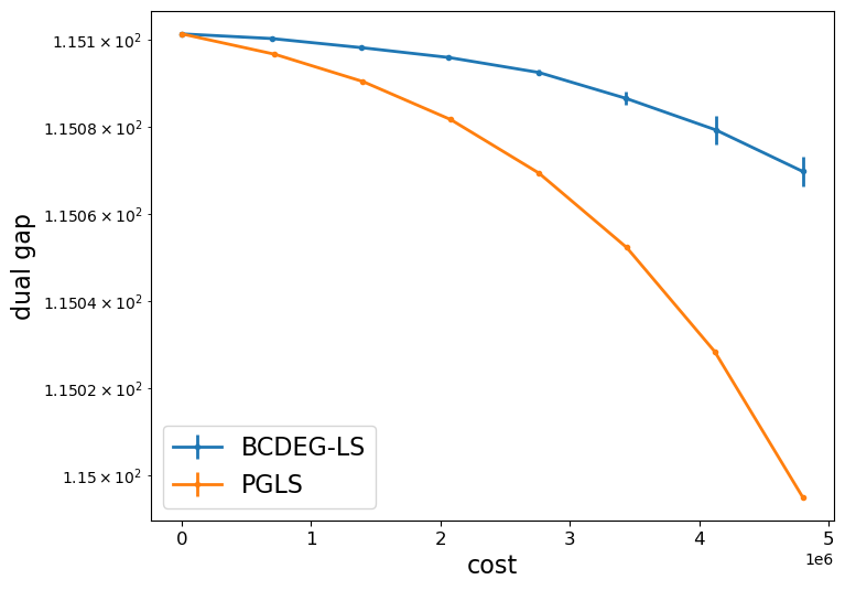
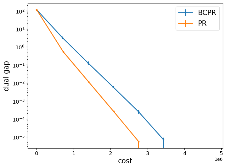
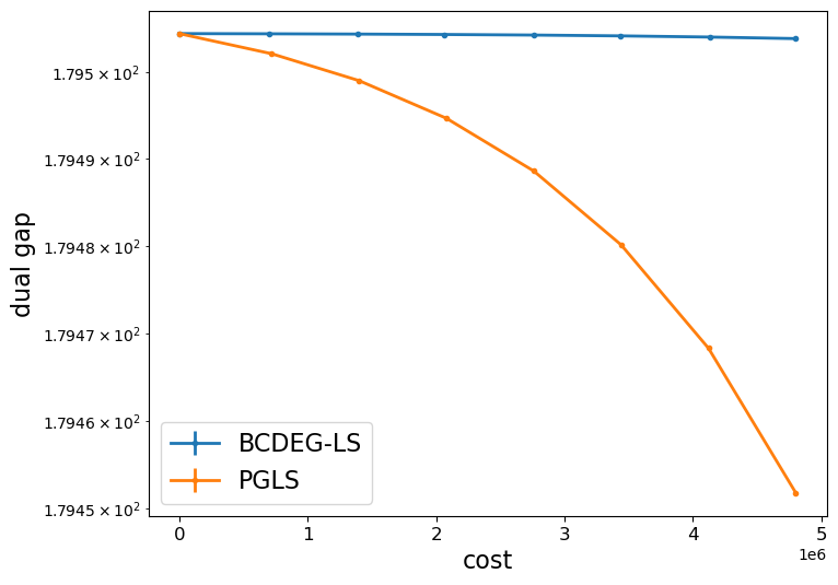
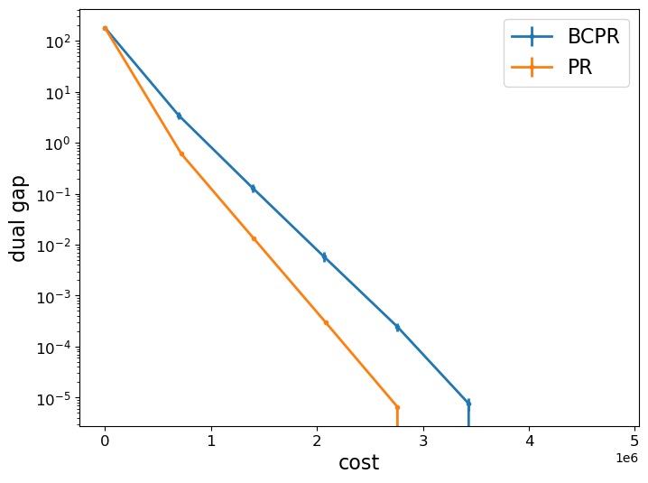
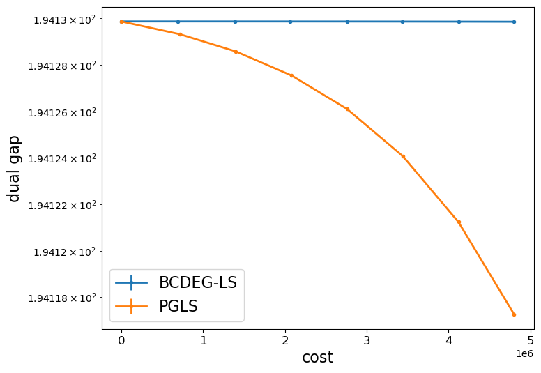
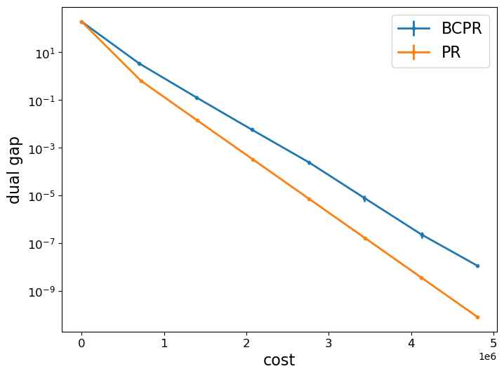
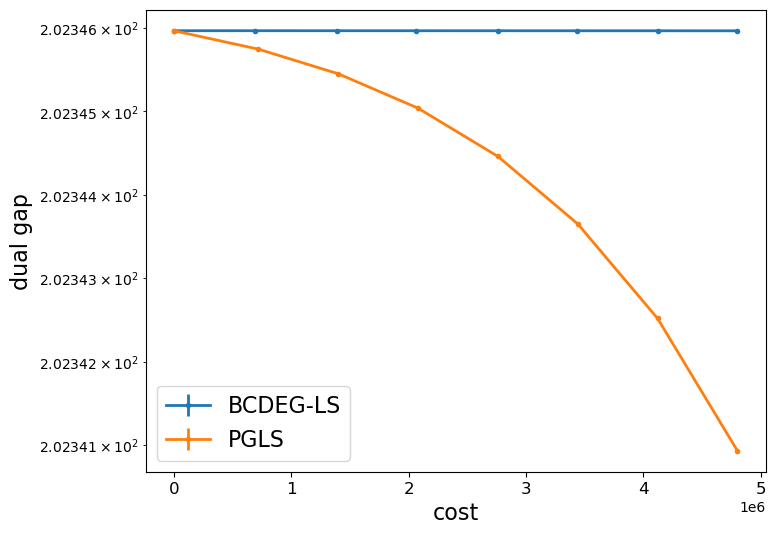
Figure 4: Performance on more simulated instances with CES utilities. ($\hat{v}=0.4,0.6,0.8,1.0$ from top to bottom). The plot setup is the same as in Fig. 1.

Appendix F Discussion on wall-clock running times

In this paper, we compare different algorithms based on the number of times they query for a buyer-item valuation (i.e. the number of accesses to cells of the valuation matrix). In this sense, if we count one query as one unit cost, then item-block algorithms (BCDEG, BCDEG-LS) cost $n$ units in each iteration, buyer-block algorithms (BCPR, A-BCPR, BCPR-LS) cost $m$ units in each iteration, and full gradient algorithms (PGLS, PR) cost $nm$ units in each iteration. Another way to compare these algorithms would be to compare wall-clock running times. In this section we justify our choice of measuring valuation accesses instead.

For the projected-gradient style methods (the full deterministic method and BCDEG variants), they each perform one $n$-dimensional projection for every $n$ units of work, and thus all these methods are directly comparable in terms of our measure. Similarly, all proportional-response-style algorithms perform the same amount of work for every $m$ queries made. Thus they are also directly comparable in terms of our measure. When comparing projected-gradient-style methods to PR-style methods, there is a difference in that projection is required in the former. Yet in practice it is known that efficient implementations of the best projection-style algorithms tend to run in linear time as well  (Condat 2016). Thus cross comparisons should also be fair. The main reason why wall-clock might differ from our measure is due to efficiency of the implementation. All our experiments are implemented in python. For that reason, deterministic methods could have an advantage over block-coordinate methods in terms of wall clock, since NumPy and MKL enable highly-optimized matrix/vector operations. In turn, this means that deterministic methods can spend more time ‘in C’ as opposed to ‘in python.’ If all algorithms are implemented without highly optimized matrix operations that exploit multi-core CPUs, experimental results on wall-clock running times will be consistent with our query-based complexity cost. Similarly, if they are all optimized fully to take advantage of hardware, parallelization, etc., we can still expect similar results.

References

- Arnsperger (1994) Arnsperger, C. 1994. Envy-freeness and distributive justice. Journal of Economic Surveys, 8(2): 155–186.
- Attouch, Bolte, and Svaiter (2013) Attouch, H.; Bolte, J.; and Svaiter, B. F. 2013. Convergence of descent methods for semi-algebraic and tame problems: proximal algorithms, forward–backward splitting, and regularized Gauss–Seidel methods. Mathematical Programming, 137(1): 91–129.
- Aziz and Ye (2014) Aziz, H.; and Ye, C. 2014. Cake cutting algorithms for piecewise constant and piecewise uniform valuations. In International Conference on Web and Internet Economics, 1–14. Springer.
- Barman, Krishnamurthy, and Vaish (2018) Barman, S.; Krishnamurthy, S. K.; and Vaish, R. 2018. Finding fair and efficient allocations. In Proceedings of the 2018 ACM Conference on Economics and Computation, 557–574.
- Bauschke, Bolte, and Teboulle (2017) Bauschke, H. H.; Bolte, J.; and Teboulle, M. 2017. A descent lemma beyond Lipschitz gradient continuity: first-order methods revisited and applications. Mathematics of Operations Research, 42(2): 330–348.
- Beck and Tetruashvili (2013) Beck, A.; and Tetruashvili, L. 2013. On the convergence of block coordinate descent type methods. SIAM journal on Optimization, 23(4): 2037–2060.