Temporal regularity of the solution to the incompressible Euler equations in the end-point critical Triebel-Lizorkin space $F^{d+1}_{1,\infty}(\mathbb{R}^{d})$

Abstract.

An evidence of temporal dis-continuity of the solution in $F^{s}_{1,\infty}(\mathbb{R}^{d})$ is presented, which implies the ill-posedness of the Cauchy problem for the Euler equations. Continuity and weak-type continuity of the solutions in related spaces are also discussed.

1. Introduction

The perfect incompressible inviscid fluid is governed by the Euler equations:

(1.1) $$\frac{\partial}{\partial t}\;u+(u,\nabla)u =-\nabla p$$

(1.2) $$\mbox{div }u =0.$$

Here $u(x,t)=(u_{1},u_{2},\cdots,u_{d})$ is the velocity of a fluid flow and $p(x,t)$ is the scalar pressure.

Existence and uniqueness theories of solutions of the 2 or 3 dimensional Euler equations have been worked on by many mathematicians and physicists. For a detailed survey of this issue, we refer [1], [3], [4], [5], [6], [7] and references therein. Bourgain and Li proved strong ill-posedness results for the Euler equations associated with initial data in (borderline) Besov spaces, Sobolev spaces or the space $C^{m}$. For the survey of the ill-posedness issue, we refer [3], [4].

This paper presents the ill-posedness of the solution in the end-point critical Triebel-Lizorkin space $F^{d+1}_{1,\infty}(\mathbb{R}^{d})$. It is reported in [10] that the solution of Euler equations stays locally in the space $F^{s}_{1,\infty}(\mathbb{R}^{d})$ (for $s\geq d+1$) without any sudden singularity in time, and its temporal propagation is, however, somehow rough in the sense that the solution may not be continuous in time. In this paper, we present a new example of initial velocity to demonstrate this phenomenon.

Bourgain and Li provided nice examples to explain sudden norm inflation of nearby solutions in borderline Sobolev spaces, and several analysts have also reported some examples to observe the norm inflation. Our example is rather simple and focuses on the direct reason why the inflation occurs in the Triebel-Lizorkin spaces. We try to explain what situation, in the frequency space, causes the solution to lose its regularity instantaneously. The spacial frequency space may be a very good place to observe the temporal regularity of the solution, and this is one of the reasons why we concentrate on the special end-point critical Triebel-Lizorkin space $F^{d+1}_{1,\infty}(\mathbb{R}^{d})$.

The space $F^{d+1}_{1,\infty}(\mathbb{R}^{d})$ is a proper subspace of $B^{1}_{\infty,1}(\mathbb{R}^{d})$. It has been reported in [8] that the solution $u:[0,T]\to F^{d+1}_{1,\infty}(\mathbb{R}^{d})$ uniquely exists and is continuous with respect to $B^{1}_{\infty,1}$-norm, but our result says that it is not continuous with respect to $F^{d+1}_{1,\infty}$-norm for a certain initial velocity $u_{0}\in F^{d+1}_{1,\infty}(\mathbb{R}^{d})$. In other words, even though an Euler flow stays locally in $F^{d+1}_{1,\infty}(\mathbb{R}^{d})$ and moves continuously inside $B^{1}_{\infty,1}(\mathbb{R}^{d})$, it may get suddenly wild in the proper subspace $F^{d+1}_{1,\infty}(\mathbb{R}^{d})$. The well- or ill-posedness results of the critical spaces do not have any direct implications to Euler dynamics of sub-critical and super-critical spaces. When it comes to the temporal continuity, the major difference between the space $F^{s}_{1,\infty}(\mathbb{R}^{d})$ and the space $B^{1}_{\infty,1}(\mathbb{R}^{d})$ is the possibility of the smooth approximations.

We discuss the continuity and weak-type continuity with values in the nearby spaces $F^{s-\varepsilon}_{1,\infty}(\mathbb{R}^{d})$ and the space $F^{s}_{1,\infty}(\mathbb{R}^{d})$, respectively. These weak-type continuities are under the same line of observing the norm inflation of solutions.

The (strong) continuity of the solution with respect to $F^{s-\varepsilon}_{1,\infty}$-norm ($\varepsilon>0$) is proved in Section 3.1 and a weak-type continuity of the solution is discussed in Section 3.3. A counterexample for the discontinuity of the solution with values in the space $F^{s}_{1,\infty}(\mathbb{R}^{d})$ is placed in Section 3.2.

Notations: Throughout this paper,

• $d$ always represents a dimensional integer greater than or equal to $2$

• for $x\in\mathbb{R}^{d}$, $x_{i}$ is the $i$-th component of $x$

• $\displaystyle\frac{\partial f}{\partial x_{k}}=\partial_{x_{k}}f$ or simply $\partial_{k}f$

• for $k>0$ and a function $\phi$ on $\mathbb{R}^{d}$, $[\phi]_{k}(x):=k^{d}\phi(kx)$ for $x\in\mathbb{R}^{d}$

• for $f\in\mathcal{S}({\mathbb{R}}^{d})$, the Fourier transform $\hat{f}={\mathcal{F}}(f)$ of $f$ on ${\mathbb{R}}^{d}$ is defined by

  $$\hat{f}(\xi)={\mathcal{F}}(f)(\xi)=\int_{{\mathbb{R}}^{n}}f(x)e^{-ix\cdot\xi}\,dx$$

• the notation $X\lesssim Y$ means that $X\leq CY$, where $C$ is a fixed but unspecified constant. Unless explicitly stated otherwise, $C$ may depend on the dimension $d$ and various other parameters (such as exponents), but not on the functions or variables $(u,v,f,g,x_{i},\cdots)$ involved.

2. Preliminaries and the main theorem

Let $\mathcal{S}(\mathbb{R}^{d})$ denote the Schwartz class. We consider a nonnegative radial function $\chi\in\mathcal{S}(\mathbb{R}^{d})$ satisfying $\mbox{supp}\>\chi\subset\{\xi\in{\mathbb{R}}^{d}:|\xi|\leq 1\}$, and $\chi=1$ for $|\xi|\leq\frac{3}{4}$. Set $h_{j}(\xi):=\chi(2^{-j-1}\xi)-\chi(2^{-j}\xi)$ and let $\varphi_{j}$ and $\Phi$ be defined by $\varphi_{j}:=\mathcal{F}^{-1}(h_{j})$ and $\Phi:=\mathcal{F}^{-1}(\chi)$. For any $f\in\mathcal{S}^{\prime}(\mathbb{R}^{d})$, we define the operators $\Delta_{j}$ and $\dot{\Delta}_{j}$ by

$$\Delta_{j}f=\begin{cases}\hat{\varphi_{j}}(D)f=\varphi_{j}\ast f&\text{for }j\geq 0\\ \hat{\Phi}(D)f=\Phi\ast f&\text{for }j=-1\\ 0&\text{for }j\leq-2,\end{cases}\quad\dot{\Delta}_{j}f=\begin{cases}\Delta_{j}f&\text{for }j\geq 0\\ \hat{\varphi_{j}}(D)f=\varphi_{j}\ast f&\text{for }j\leq-1,\end{cases}$$

respectively. The partial sum operator $S_{k}f$ is defined as $\displaystyle{S_{k}f=\sum_{j=-\infty}^{k}\Delta_{j}f}$.

For $s\in\mathbb{R}$, the homogeneous Triebel-Lizorkin space $\dot{F}_{1,\infty}^{s}(\mathbb{R}^{d})$ is the collection of all tempered distributions $f\in\mathcal{S}^{\prime}(\mathbb{R}^{d})$ modulo polynomials such that

$$\|f\|_{\dot{F}_{1,\infty}^{s}}:=\int_{\mathbb{R}^{d}}\underset{j\in\mathbb{Z}}{\sup}\left|2^{js}\dot{\Delta}_{j}f\right|(x)dx<\infty,$$

and the nonhomogeneous Triebel-Lizorkin space $F_{1,\infty}^{s}(\mathbb{R}^{d})$ is the space of all tempered distributions $f\in\mathcal{S}^{\prime}(\mathbb{R}^{d})$ obeying

(2.1) $$\|f\|_{F_{1,\infty}^{s}}:=\int_{\mathbb{R}^{d}}\underset{j\in\mathbb{Z}}{\sup}\left|2^{js}{\Delta}_{j}f\right|(x)dx<\infty.$$

We observe that for $s>0$, the Triebel-Lizorkin norm $\|f\|_{F_{1,\infty}^{s}}$ is equivalent to the nonhomogeneous norm

(2.2) $$\|f\|_{L^{1}}+\|f\|_{\dot{F}_{1,\infty}^{s}}.$$

We present some a-priori estimates with respect to the spaces $\dot{F}_{1,\infty}^{s}(\mathbb{R}^{d})$ and $F_{1,\infty}^{s}(\mathbb{R}^{d})$ which are used in this manuscript. The following properties and their proofs can be found in [10].

Remark 2.1.

Let $s>0$. Let $f$ and $g$ be scalar functions and $u$ be a vector field.
1. One has

$$\|fg\|_{{F}_{1,\infty}^{s}}\lesssim\|f\|_{L^{\infty}}\|g\|_{{F}_{1,\infty}^{s}}+\|g\|_{L^{\infty}}\|f\|_{{F}_{1,\infty}^{s}}.$$

2. The Leray projection $\mathbb{P}:=u-\nabla\Delta^{-1}(\nabla\cdot u)$ is continuous on $\dot{F}_{1,\infty}^{s}(\mathbb{R}^{d})$, that is,

$$\|\mathbb{P}u\|_{\dot{F}_{1,\infty}^{s}}\lesssim\|u\|_{\dot{F}_{1,\infty}^{s}}.$$

3. For the pressure $p$ in (1.1) defined as $p:=(-\Delta)^{-1}\mathrm{div}((u,\,\nabla)u)$, we have

$$\|\nabla p\|_{L^{1}}\lesssim\|u\|_{{W}^{1,\infty}}\|u\|_{\dot{F}_{1,\infty}^{s}}.$$

Wherein all of the right hand sides are finite.

We now state our main result:

Theorem 2.2.

Let $u$ be the solution of the Euler equations (1.1) in $L^{\infty}([0,T];F_{1,\infty}^{s})$ with initial velocity $u(0)=u_{0}\in F_{1,\infty}^{s}(\mathbb{R}^{d})$ for $s\geq d+1$.

1. (Temporal continuity with values in ${F}^{s-\varepsilon}_{1,\infty}(\mathbb{R}^{d})$) For any $\varepsilon>0$, $u:[0,T]\to{F}^{s-\varepsilon}_{1,\infty}(\mathbb{R}^{d})$ is continuous.
2. (Discontinuity with values in ${F}^{s}_{1,\infty}(\mathbb{R}^{d})$) There exists an initial velocity $u_{0}\in F_{1,\infty}^{s}(\mathbb{R}^{d})$ such that $u:[0,T]\to{F}^{s}_{1,\infty}(\mathbb{R}^{d})$ is not continuous.
3. (Weak type continuity with values in ${F}^{s}_{1,\infty}(\mathbb{R}^{d})$) For any sequence of real numbers $\{k_{j}\}_{j=-1}^{\infty}\in\ell^{1}$, the function

(2.3) $$t\mapsto\left\|\sum_{j=-1}^{\infty}2^{js}k_{j}\Delta_{j}u(\cdot,t)\right\|_{L^{1}}$$

is continuous on $[0,T]$.

The third property states that the solution $u:[0,T]\to F_{1,\infty}^{s}$ is weak*-continuous with respect to (pointwise) $\ell^{\infty}$-norm, and it is, however, strong-continuous with respect to $L^{1}$-norm.

Remark 2.3.

By virtue of time–reversibility of Euler systems, all of the time intervals $[0,T]$ in the statements of the main theorem can be replaced by $[-T,T]$ and the time interval $[0,\infty)$ can also be replaced by the whole time $\mathbb{R}$ for the 2-D solution.

3. Temporal regularity of the solution

We now investigate the temporal regularity of the solution to the Euler equations in $F_{1,\infty}^{s}(\mathbb{R}^{d})$. The (unique local-in-time) solution in the Besov space $B^{1}_{\infty,1}(\mathbb{R}^{d})$ is known to be continuous. However, the proper subspaces ${F}^{s}_{1,\infty}(\mathbb{R}^{d})$ ($s\geq d+1$) of the space $B^{1}_{\infty,1}(\mathbb{R}^{d})$ permit only rougher temporal regularity. In this section, we carry out a detailed explanation.

We first recall that the solution $u$ of the Euler equations (1.1) with initial velocity $u_{0}\in{F}^{s-\varepsilon}_{1,\infty}(\mathbb{R}^{d})$ is located inside the space $L^{\infty}([0,T_{0});F_{1,\infty}^{s})$ with $T_{0}:=\frac{1}{C^{2}_{0}\|u_{0}\|_{F_{1,\infty}^{s}}}$ (page 9 in [10]). Moreover, the velocity field $u$ is dominated by a fractional function $y(t)$;

$$\sup_{0\leq\tau\leq t}\|u(\tau)\|_{F_{1,\infty}^{s}}\leq\frac{C_{0}\|u_{0}\|_{F_{1,\infty}^{s}}}{1-tC^{2}_{0}\|u_{0}\|_{F_{1,\infty}^{s}}}:=y(t),\quad 0<t<T_{0}.$$

(The argument can be found in [10]). Hereafter we fix a positive time $T_{1}$ with $T_{1}<T_{0}$.

3.1. Continuity of the solution with values in ${F}^{s-\varepsilon}_{1,\infty}(\mathbb{R}^{d})$

We prove the continuity of the solution $u:[0,T_{1}]\to{F}^{s-\varepsilon}_{1,\infty}(\mathbb{R}^{d})$ ($\varepsilon>0$).

We take ${\Delta}_{j}$ and then the Leray projection $\mathbb{P}$ on both sides of the Euler equations to get

(3.1) $$\partial_{t}(\mathbb{P}{\Delta}_{j}u)=-{\Delta}_{j}\mathbb{P}(u,\,\nabla)u.$$

Integrate both sides of (3.1) to get

$$\Delta_{j}u(x,\,t)=\Delta_{j}u_{0}-\int_{0}^{t}\Delta_{j}\mathbb{P}(u,\,\nabla)u(\tau)d\tau.$$

Then Remark 2.1 implies that for any $t_{1},t_{2}\in[0,T_{1}]$ with $t_{1}\leq t_{2}$,

$$\|u(t_{1})-u(t_{2})\|_{F_{1,\,\infty}^{s-1}} \leq\int_{t_{1}}^{t_{2}}\|\mathbb{P}(u,\,\nabla)u\|_{F_{1,\,\infty}^{s-1}}d\tau$$

$$\lesssim\int_{t_{1}}^{t_{2}}\left(\|\mathbb{P}(u,\,\nabla)u\|_{\dot{F}_{1,\,\infty}^{s-1}}+\|\mathbb{P}(u,\,\nabla)u\|_{L^{1}}\right)d\tau$$

$$\lesssim\int_{t_{1}}^{t_{2}}\left(\|(u,\,\nabla)u\|_{{F}_{1,\,\infty}^{s-1}}+\|\nabla p\,\|_{L^{1}}\right)d\tau$$

$$\lesssim|t_{1}-t_{2}|,$$

which yields that $u\in{\rm Lip}([0,T_{1}];F^{s-1}_{1,\infty})$.

For $\ell\in\mathbb{N}$, we set $\displaystyle{u_{\ell}:=S_{\ell}\,u}=\displaystyle{\sum_{j=-\infty}^{\ell}\Delta_{j}f}$. For any $t_{1},t_{2}\in[0,T_{1}]$, from the estimate that (we recall that $\Delta_{j}=0$ for $j\leq-2$)

$$\|u_{\ell}(t_{1})-u_{\ell}(t_{2})\|_{{F}^{s^{\prime}}_{1,\infty}}$$

$$=\left\|\sup_{j\in\mathbb{Z}}\left|2^{js^{\prime}}\Delta_{j}\sum_{j=-\infty}^{\ell}\Delta_{k}(u(t_{1})-u(t_{2}))\right|\right\|_{{L}^{1}}$$

$$\lesssim\left\|\left(\sup_{-1\leq j\leq\ell+1}2^{j(1-s+s^{\prime})}\right)\sup_{j\in\mathbb{Z}}\left|2^{j(s-1)}\Delta_{j}(u(t_{1})\!-\!u(t_{2}))\right|\right\|_{{L}^{1}}$$

$$\lesssim|t_{1}-t_{2}|,$$

we can deduce that each $u_{\ell}:[0,T_{1}]\to{F}^{s^{\prime}}_{1,\infty}(\mathbb{R}^{d})$ is Lipschitz continuous for any $s^{\prime}\in\mathbb{R}$.

Now, for $t\in[0,T_{1}]$, we have

$$\|u(t)-u_{\ell}(t)\|_{{F}^{s-\varepsilon}_{1,\infty}} =\left\|\sup_{j\in\mathbb{Z}}\left|2^{j(s-\varepsilon)}\Delta_{j}\left(\sum_{k=\ell+1}^{\infty}\Delta_{k}u(t)\right)\right|\right\|_{{L}^{1}}$$

$$\lesssim 2^{-\ell\varepsilon}\left\|u\right\|_{L^{\infty}([0,T_{1}];F_{1,\infty}^{s})}\to 0\quad\mbox{as }\ell\to\infty,$$

and so the sequence $\left\{u_{\ell}\right\}_{\ell\in\mathbb{N}}$ converges uniformly to $u$ on $[0,T_{1}]$ with values in ${F}^{s-\varepsilon}_{1,\infty}(\mathbb{R}^{d})$. Hence the uniform limit $u:[0,T_{1}]\to{F}^{s-\varepsilon}_{1,\infty}(\mathbb{R}^{d})$ is continuous. $\Box$

Unfortunately the continuity of the solution $u$ is, however, broken down with respect to ${F}^{s}_{1,\infty}$-norm. In the next section, a counter-example is presented in detail.

3.2. Lack of temporal continuity of the solution in ${F}^{s}_{1,\infty}(\mathbb{R}^{d})$

We present a counter-example $u$ of the solution with initial velocity $u_{0}$ in $F_{1,\infty}^{s}(\mathbb{R}^{d})$ which is not continuous on $[0,T_{1}]$, and is not continuous at $t=0$ in particular.

We summon the radial symmetric smooth nonnegative mother function $\chi$ from page 2. We translate $\chi$ along the $\xi_{1}$-axis in the positive direction by $2^{j}(1+\frac{1}{4})$, and then rotate it by $\frac{\pi}{6}$ with respect to the origin on the $\xi_{1}$$\xi_{2}$ plane to get $\widehat{a_{j}}$ for $j=1,2,3,\cdots$. That is, for $j=1,2,3,\cdots$,

$$\widehat{a_{j}}(\xi)=\chi\left(\xi-\xi^{j}\right),$$

where we set

$$\xi^{j}:=5\cdot 2^{j-2}\left(\frac{\sqrt{3}}{2},\frac{1}{2},0,\cdots,0\right),\quad j\in\mathbb{Z}.$$

We let $\widehat{a_{0}}\equiv 0$ and choose a nonnegative smooth function $\widehat{a_{-1}}\in\mathcal{S}(\mathbb{R}^{d})$ satisfying

$$\mbox{supp}\>\widehat{a_{-1}}\subseteq B(\xi^{-1},2^{-3})\quad\mbox{ and }\quad\int_{\mathbb{R}^{d}}(\xi_{1}-\sqrt{3}\xi_{2})\widehat{a_{-1}}(\xi)d\xi\neq 0.$$

(Note that the rotation followed by the translation allows that the supports of $\hat{a_{j}}$ are located in the first quadrant of the $\xi_{1}$$\xi_{2}$ plane.) By the construction, we have that

$$\widehat{a_{j}}(\xi)=\widehat{a_{j}}(\xi)h_{j}(\xi),$$

where $h_{j}$ ($j=-1,0,1,\cdots$) are the generating functions defined at page 2. We denote $a_{j}:=\mathcal{F}^{-1}(\widehat{a_{j}})$ ($j=-1,0,1,\cdots$) and define

$$\alpha(x):=\sum_{j=-1}^{\infty}2^{-j(s+1)}a_{j}(x)\qquad\mbox{for }x\in\mathbb{R}^{d}.$$

We consider the initial velocity $u_{0}$ defined by

$$u_{0}(x):=\left(-\partial_{x_{2}}\alpha(x),\partial_{x_{1}}\alpha(x),0,\cdots,0\right)$$

for $x=(x_{1},x_{2},\cdots,x_{d})\in\mathbb{R}^{d}$. Then it can be easily seen that $\alpha$ is well-defined and $u_{0}$ is divergence free.

Lemma 3.1.

The vector field $u_{0}$ is in $F_{1,\infty}^{s}(\mathbb{R}^{d})$.

Proof. For $\ell=1,2$, we have

$$\sup_{j\geq-1}\left|\Delta_{j}2^{js}\partial_{x_{\ell}}\alpha(x)\right|\!=\!\sup_{j\geq-1}\left|[2^{-j}\partial_{x_{\ell}}a_{j}(x)\right|\lesssim\!|\partial_{x_{\ell}}a_{-1}(x)|\!+\!\sup_{j\geq 1}\left|[2^{-j}\partial_{x_{\ell}}a_{j}(x)\right|.$$

It is obvious that $\partial_{x_{\ell}}a_{-1}$ is in $L^{1}(\mathbb{R}^{d})$. For $j\in\mathbb{N}$, we observe that

$$2^{-j}\left|\partial_{x_{\ell}}a_{j}(x)\right|=2^{-j}\left|\partial_{x_{\ell}}\left(e^{i5\cdot 2^{j-3}(\sqrt{3}x_{1}+x_{2})}\Phi(x)\right)\right|\lesssim\left|\Phi(x)\right|+2^{-j}\left|\Phi_{x_{\ell}}(x)\right|$$

($\ell=1,2$). Therefore we conclude that $\int_{\mathbb{R}^{d}}\sup_{j\geq-1}\left|\Delta_{j}2^{js}\partial_{x_{\ell}}\alpha(x)\right|dx$ is finite. $\Box$

Let $u$ be the solution in the space $L^{\infty}([0,T_{1}];F_{1,\infty}^{s})$ with the initial velocity $u_{0}$. Then from the fact that

$$\hat{u}(\xi^{k},0)=\widehat{u_{0}}(\xi^{k})=i5\cdot 2^{-ks-3}\left(-1,\sqrt{3},0,\cdots,0\right)=:2^{-ks}{\bf c}_{0},$$

we have that for $0<t<T_{1},$

$$\hat{u}(\xi^{k},t) =\hat{u}(\xi^{k},0)+\int_{0}^{t}\mathcal{F}(\mathbb{P}(u,\nabla)u)(\xi^{k},\tau)d\tau$$

$$=2^{-ks}{\bf c}_{0}+t\mathcal{F}(\mathbb{P}(u_{0},\nabla)u_{0})(\xi^{k})$$

(3.2) $$\qquad+\int_{0}^{t}\left(\mathcal{F}(\mathbb{P}(u,\nabla)u)(\xi^{k},\tau)-\mathcal{F}(\mathbb{P}(u_{0},\nabla)u_{0})(\xi^{k})\right)d\tau.$$

In order to find a lower bound of (3.2), we present some computational lemmas for the right hand side of (3.2).

Lemma 3.2.

We have a constant vector ${\bf c}_{1}$ independent on $k$ and a vector ${\bf c}_{2}(k)$ depending upon $k$ such that

(3.3) $$2^{sk}\times\mathcal{F}(\mathbb{P}(u_{0},\nabla)u_{0})(\xi^{k})=2^{k}\left({\bf c}_{1}+{\bf c}_{2}(k)\right)$$

and ${\bf c}_{2}(k)\to\bf{0}$ as $k$ goes to infinity.

Proof. We have

$$\mathcal{F}(\mathbb{P}(u_{0},\nabla)u_{0})(\xi^{k})$$

(3.4) $$=\left(\frac{\sqrt{3}-1}{4}\mathcal{F}((u_{0},\!\nabla)\alpha_{x_{2}})(\xi^{k}),\frac{3-\sqrt{3}}{4}\mathcal{F}((u_{0},\!\nabla)\alpha_{x_{1}})(\xi^{k}),0,\cdots,0\right)$$

by considering the symbol of the Leray projection $\mathbb{P}$

$$\widehat{\mathbb{P}(u)}=\hat{u}-\left(\sum_{\ell=1}^{d}\xi_{\ell}\right)\frac{\left(\xi_{1}\widehat{u^{1}},\xi_{2}\widehat{u^{2}},\cdots,\xi_{d}\widehat{u^{d}}\right)}{|\xi|^{2}}$$

at the point $\xi^{k}$. For $\ell=1,2$, some computations and the cancellation of a common term yield

$$\mathcal{F}\left((u_{0},\nabla)\alpha_{x_{\ell}}\right)(\xi^{k})$$

$$=(2\pi)^{-d}i\left[(\xi_{2}\hat{\alpha})*(\xi_{1}\xi_{\ell}\,\hat{\alpha})-(\xi_{1}\hat{\alpha})*(\xi_{2}\xi_{\ell}\,\hat{\alpha})\right](\xi^{k})$$

$$=(2\pi)^{-d}i5\;2^{k-3}\!\!\int_{\mathbb{R}^{d}}\!\!\hat{\alpha}(\xi^{k}-\xi)\xi_{1}\xi_{\ell}\,\hat{\alpha}(\xi)d\xi\!-\!i5\sqrt{3}\;2^{k-3}\!\!\int_{\mathbb{R}^{d}}\!\!\hat{\alpha}(\xi^{k}-\xi)\xi_{2}\xi_{\ell}\,\hat{\alpha}(\xi)d\xi$$

(3.5) $$=(2\pi)^{-d}i5\;2^{k-3}\!\!\int_{\mathbb{R}^{d}}\!\!\left(\xi_{1}-\sqrt{3}\xi_{2}\right)\xi_{\ell}\,\hat{\alpha}(\xi^{k}-\xi)\hat{\alpha}(\xi)d\xi.$$

We consider the supports of $\hat{\alpha}(\cdot)$ and $\hat{\alpha}(\xi^{k}-\cdot)$ in the frequency space(see Figure 1), and observe that only three components of the common supports survive. Hence we can write

$$\int_{\mathbb{R}^{d}}\left(\xi_{1}-\sqrt{3}\xi_{2}\right)\xi_{\ell}\,\hat{\alpha}(\xi^{k}-\xi)\hat{\alpha}(\xi)d\xi$$

$$=2^{-(k-1)(s+1)}\int_{B(\xi^{-1},2^{-3})}\left(\xi_{1}-\sqrt{3}\xi_{2}\right)\xi_{\ell}\,\widehat{a_{k}}\left(\xi^{k}-\xi\right)\widehat{a_{-1}}(\xi)d\xi$$

$$\phantom{....}+2^{(-2k+2)(s+1)}\int_{B(\xi^{k-1},1)}\left(\xi_{1}-\sqrt{3}\xi_{2}\right)\xi_{\ell}\,\widehat{a_{k-1}}\left(\xi^{k}-\xi\right)\widehat{a_{k-1}}(\xi)\,d\xi$$

(3.6) $$\phantom{....}+2^{-(k-1)(s+1)}\!\!\int_{B(\xi^{k}-\xi^{-1},2^{-3})}\!\!\left(\xi_{1}-\sqrt{3}\xi_{2}\right)\xi_{\ell}\,\widehat{a_{-1}}\left(\xi^{k}-\xi\right)\widehat{a_{k}}(\xi)d\xi.$$

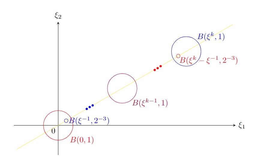
Figure 1. supports of $\hat{\alpha}(\cdot)$ (= the blue disks) and $\hat{\alpha}(\xi^{k}-\cdot)$ (= the red disks)

Then we look into the integral of each term, successively. From the fact that $\chi(\xi)=1$ if $|\xi|\leq\frac{3}{4}$, we note that

$$\widehat{a_{k}}\left(\xi^{k}-\xi\right)=\chi\left(-\xi\right)=1,\quad\mbox{ for }\;\xi\in B(\xi^{-1},2^{-3}).$$

Hence we have

$$\int_{B(\xi^{-1},2^{-3})} \left(\xi_{1}-\sqrt{3}\xi_{2}\right)\xi_{\ell}\,\widehat{a_{k}}\left(\xi^{k}-\xi\right)\widehat{a_{-1}}(\xi)d\xi$$

(3.7) $$=\int_{B(\xi^{-1},2^{-3})}\left(\xi_{1}-\sqrt{3}\xi_{2}\right)\xi_{\ell}\,\widehat{a_{-1}}(\xi)d\xi.$$

Similarly, we obtain

$$\int_{B(\xi^{k-1},1)} \left(\xi_{1}-\sqrt{3}\xi_{2}\right)\xi_{\ell}\,\widehat{a_{k-1}}\left(\xi^{k}-\xi\right)\widehat{a_{k-1}}(\xi)\,d\xi$$

$$=\int_{B(\xi^{k-1},1)}\left(\xi_{1}-\sqrt{3}\xi_{2}\right)\xi_{\ell}\,\chi\left(-\xi+\xi^{k-1}\right)\chi\left(\xi-\xi^{k-1}\right)d\xi$$

(3.8) $$=\int_{B(0,1)}\left(\eta_{1}-\sqrt{3}\eta_{2}\right)\eta_{\ell}\,\chi^{2}(\eta)d\eta$$

and by taking into account the support of $\chi$ once more, we get

$$\int_{B(\xi^{k}-\xi^{-1},2^{-3})} \left(\xi_{1}-\sqrt{3}\xi_{2}\right)\xi_{\ell}\,\widehat{a_{-1}}\left(\xi^{k}-\xi\right)\widehat{a_{k}}(\xi)d\xi$$

$$=\int_{B(\xi^{k}-\xi^{-1},2^{-3})}\left(\xi_{1}-\sqrt{3}\xi_{2}\right)\xi_{\ell}\,\widehat{a_{-1}}\left(\xi^{k}-\xi\right)d\xi d\xi$$

$$=\int_{B(\xi^{-1},2^{-3})}\left(\eta_{1}-\sqrt{3}\eta_{2}\right)\eta_{\ell}\;\widehat{a_{-1}}(\eta)d\eta$$

(3.9) $$\quad-5\sqrt{3}^{2-\ell}2^{k-3}\int_{B(\xi^{-1},2^{-3})}\left(\eta_{1}-\sqrt{3}\eta_{2}\right)\widehat{a_{-1}}(\eta)d\eta.$$

At the last equality, terms are canceled by the substitution $\eta=\xi^{k}-\xi$ together with the orientation induced by $d\eta=(-1)^{d}d\xi$. Then we plug the identities (3.7), (3.8), (3.9) into (3.6) to find a constant $c^{\ell}_{1}$ and a function $c^{\ell}_{2}(k)$ of $k$ such that

(3.10) $$\int_{\mathbb{R}^{d}}\left(\xi_{1}-\sqrt{3}\xi_{2}\right)\xi_{\ell}\,\hat{\alpha}(\xi^{k}-\xi)\hat{\alpha}(\xi)d\xi=2^{-ks}\left(c^{\ell}_{1}+c^{\ell}_{2}(k)\right)$$

and $c^{\ell}_{2}(k)\to 0$ as $k$ goes to infinity ($\ell=1,2$). Then we place the identity (3.10) into (3.5), and (3.4) to get the result (3.3). $\Box$

Lemma 3.3.

For divergence free vector fields $u,v$ in $F_{1,\infty}^{s}(\mathbb{R}^{d})$ and for a positive integer $k$, we have

$$\|\Delta_{k}(u,\nabla)v\|_{L^{1}}\lesssim 2^{k(1-s)}\|u\|_{{F}_{1,\infty}^{s}}\|v\|_{{F}_{1,\infty}^{s}}.$$

Proof. Divergence-free condition of $u$ delivers that

(3.11) $$\|\Delta_{k}(u,\nabla)v\|_{L^{1}}\lesssim 2^{k}\|\Delta_{k}(u\otimes v)\|_{L^{1}}$$

with $u:=(u_{1},u_{2},\cdots,u_{d})$ and $v:=(v_{1},v_{2},\cdots,v_{d})$. For the simplicity, we denote $f:=u_{i}$, and $g:=v_{j}$. Then the Bony’s paraproduct decomposition for $fg$ can be written as

$$fg={T}_{f}g+{T}_{g}f+{R}\left(f,\,g\right),$$

where the para-product $T_{f}g$ and the remainder $R\left(f,\,g\right)$ are defined by

$$T_{f}g:=\sum_{j\in\mathbb{Z}}S_{j-4}f\Delta_{j}g\quad\mbox{and}\quad R\left(f,\,g\right)=\sum_{\left|i-j\right|\leq 3}\Delta_{i}f\Delta_{j}g,$$

respectively [2]. Then Young’s inequality and Bernstein’s lemma yield

$$\left\|\Delta_{k}{T}_{f}g\right\|_{L^{1}} =\int_{\mathbb{R}^{d}}\left|\sum_{j=k-2}^{k+2}{\Delta}_{k}\left({S}_{j-4}f{\Delta}_{j}g\right)(x)\right|dx$$

$$\lesssim\sum_{j=k-2}^{k+2}\int_{\mathbb{R}^{d}}\left|{S}_{j-4}f{\Delta}_{j}g\right|(x)dx$$

$$\lesssim 2^{-ks}\sum_{j=k-2}^{k+2}\int_{\mathbb{R}^{d}}\left\|{S}_{j-4}f\right\|_{L^{\infty}}\left|2^{ks}{\Delta}_{j}g\right|(x)dx$$

(3.12) $$\lesssim 2^{-ks}\sum_{j=k-2}^{k+2}\|f\|_{L^{\infty}}\int_{\mathbb{R}^{d}}\underset{j\in\mathbb{Z}}{\sup}\;2^{js}\left|{\Delta}_{j}g\right|dx\lesssim 2^{-ks}\|f\|_{{F}_{1,\infty}^{s}}\|g\|_{{F}_{1,\infty}^{s}}.$$

Similarly, we can get

(3.13) $$\|{T}_{g}f\|_{{F}_{1,\infty}^{s}}\lesssim 2^{-ks}\|g\|_{{F}_{1,\infty}^{s}}\|f\|_{{F}_{1,\infty}^{s}}.$$

For the remainder term, the fact that $\mathrm{supp}\>\mathcal{F}\left(\Delta_{k}\left(\Delta_{j}f\Delta_{j+l}g\right)\right)=\emptyset$ if $j\leq k-6$ together with Young’s inequality indicates that

$$\|\Delta_{k}R(f,\,g)\|_{L^{1}} \leq\sum_{l=-3}^{3}\int_{\mathbb{R}^{d}}\left|\sum_{j=k-5}^{\infty}\Delta_{k}(\Delta_{j}f\Delta_{j+l}g)\right|(x)dx$$

$$\lesssim 2^{-ks}\sum_{l=-3}^{3}\int_{\mathbb{R}^{d}}\sum_{j=k-5}^{\infty}2^{(k-j-l)s}\left|(\Delta_{j}f)2^{(j+l)s}\Delta_{j+l}g\right|dx$$

(3.14) $$=2^{-ks}\sum_{l=-3}^{3}\int_{\mathbb{R}^{d}}\underset{k^{\prime}\in\mathbb{Z}}{\sup}\;\sum_{j=k^{\prime}-5}^{\infty}2^{(k^{\prime}-j-l)s}\left|(\Delta_{j}f)2^{(j+l)s}\Delta_{j+l}g\right|dx.$$

The integrand of (3.14) is equal to

$$\underset{k^{\prime}\in\mathbb{Z}}{\sup}\left|(a\ast b)(k^{\prime})\right|(x),$$

where the sequences $a:=\{a_{j}\}_{j\in\mathbb{Z}}$ and $b:=\{b_{j}\}_{j\in\mathbb{Z}}$ are defined by

$$a_{j}:=\begin{cases}2^{(j-l)s},&\text{if }j\leq 5\\ 0,&\text{if }j>5\end{cases},\quad b_{j}:=\left|(\Delta_{j}f)2^{(j+l)s}\Delta_{j+l}g\right|$$

for $j\in\mathbb{Z}$. Then Young’s inequality for $l^{q}$-sequences implies the estimate

$$\underset{k^{\prime}\in\mathbb{Z}}{\sup}\left|(a\ast b)(k^{\prime})\right|(x)\leq 2^{-ls}\left(\sum_{j=-\infty}^{5}2^{js}\right)\underset{j\in\mathbb{Z}}{\sup}|b_{j}|(x)\lesssim\underset{j\in\mathbb{Z}}{\sup}|b_{j}|(x).$$

Hence Höler’s inequality can be used to get

$$\|R(f,\,g)\|_{{F}_{1,\infty}^{s}} \lesssim 2^{-ks}\sum_{l=-3}^{3}\int_{\mathbb{R}^{d}}\underset{j\in\mathbb{Z}}{\sup}\;\left|(\Delta_{j}f)2^{(j+l)s}\Delta_{j+l}g\right|(x)dx$$

$$\lesssim 2^{-ks}\|f\|_{L^{\infty}}\sum_{l=-3}^{3}\int_{\mathbb{R}^{d}}\underset{j\in\mathbb{Z}}{\sup}\;|2^{(j+l)s}\Delta_{j+l}g|(x)dx$$

(3.15) $$\lesssim 2^{-ks}\|f\|_{{F}_{1,\infty}^{s}}\|g\|_{{F}_{1,\infty}^{s}}.$$

Combining the estimates (3.12), (3.13) and (3.15), we obtain

(3.16) $$\|fg\|_{{F}_{1,\infty}^{s}}\lesssim 2^{-ks}\|f\|_{{F}_{1,\infty}^{s}}\|g\|_{{F}_{1,\infty}^{s}}.$$

In all, the estimate (3.11) together with the estimate (3.16) completes the proof. $\Box$

Note that for $0\leq t\leq T_{1}$, Hausdorff-Young inequality implies that

$$2^{ks}|\hat{u}(\xi^{k},t)| =|2^{ks}h_{k}(\xi^{k})\hat{u}(\xi^{k},t)|$$

(3.17) $$\lesssim\left\|\sup_{k\geq-1}|2^{ks}\Delta_{k}u(\cdot,t)|\right\|_{L^{1}}=\|u(t)\|_{{F}_{1,\infty}^{s}}.$$

On the other hand, Hausdorff-Young inequality and Lemma 3.3 also say that

$$\left|\mathcal{F}(\mathbb{P}(u,\nabla)u)(\xi^{k},\tau)-\mathcal{F}(\mathbb{P}(u_{0},\nabla)u_{0})(\xi^{k})\right|$$

$$\lesssim\left|h_{k}(\xi^{k})\mathcal{F}((u,\nabla)u)(\xi^{k},\tau)-h_{k}(\xi^{k})\mathcal{F}((u_{0},\nabla)u_{0})(\xi^{k})\right|$$

$$\lesssim\left\|\Delta_{k}(u,\nabla)u(\tau)-\Delta_{k}(u_{0},\nabla)u_{0}\right\|_{L^{1}}$$

(3.18) $$\lesssim 2^{k(1-s)}\left(\|u(\tau)\|_{{F}_{1,\infty}^{s}}+\|u_{0}\|_{{F}_{1,\infty}^{s}}\right)\|u(\tau)-u_{0}\|_{{F}_{1,\infty}^{s}}.$$

Therefore the identity (3.2) together with (3.17) and (3.18) implies that for $0<t\leq T_{1}$,

$$\|u(t)\|_{{F}_{1,\infty}^{s}}\! \gtrsim\left|{\bf c}_{0}+t2^{k}\left({\bf c}_{1}+{\bf c}_{2}(k)\right)\right|$$

(3.19) $$\;\;-2^{k}C_{1}\!\!\int_{0}^{t}\!\!\left(\|u(\tau)\|_{{F}_{1,\infty}^{s}}+\|u_{0}\|_{{F}_{1,\infty}^{s}}\right)\|u(\tau)-u_{0}\|_{{F}_{1,\infty}^{s}}d\tau$$

for some positive real number $C_{1}$. For sufficiently large $k$, we have

$$\left|{\bf c}_{0}+t2^{k}\left({\bf c}_{1}+{\bf c}_{2}(k)\right)\right|\geq t2^{k}\left(\left|{\bf c}_{1}\right|-|{\bf c}_{2}(k)|\right)-|{\bf c}_{0}|.$$

If the solution $u$ is continuous at $t=0$, then we can choose a small time $0<t_{0}<T_{1}$ such that $\|u(\tau)-u_{0}\|_{{F}_{1,\infty}^{s}}<\frac{|{\bf c}_{1}|}{2C_{1}(\|u_{0}\|_{{F}_{1,\infty}^{s}}+\lambda(T_{1}))}$ for $0<\tau<t_{0}$. Hence we get

$$C_{1}\!\!\int_{0}^{t_{0}}\!\! \left(\|u_{0}\|_{{F}_{1,\infty}^{s}}+\|u(\tau)\|_{{F}_{1,\infty}^{s}}\right)\|u(\tau)-u_{0}\|_{{F}_{1,\infty}^{s}}d\tau$$

$$\leq C_{1}(\|u_{0}\|_{{F}_{1,\infty}^{s}}+\lambda(T_{1}))\int_{0}^{t_{0}}\!\!\|u(\tau)-u_{0}\|_{{F}_{1,\infty}^{s}}d\tau\leq\frac{t_{0}}{2}|{\bf c}_{1}|.$$

Such a situation in (3.19) with $k\to\infty$ enforces $u(t_{0})$ not to be located inside $F_{1,\infty}^{s}(\mathbb{R}^{d})$, which produces a contradiction.

In all, we cannot expect the temporal continuity of the solution with values in the space $F_{1,\infty}^{s}(\mathbb{R}^{d})$.

3.3. Temporal weak-continuity of the solution in ${F}^{s}_{1,\infty}(\mathbb{R}^{d})$

Even though we show the discontinuity of the solution $u$ for the Euler equations (1.1) in the space $F_{1,\infty}^{s}(\mathbb{R}^{d})$ in the previous section, we are able to explain a weak type continuity for the velocity $u$. In fact, we demonstrate that the solution $u:[0,T_{1}]\to{F}^{s}_{1,\infty}(\mathbb{R}^{d})$ is weakly continuous with respect to $\ell^{\infty}$-spacial space side, and strongly continuous with respect to $W^{s,1}$-spacial space side.

We define a sequence of functions $\{u_{\varepsilon}\}_{0<\varepsilon<1}$ by

$$u_{\varepsilon}(x,t):=\sum_{j=-1}^{\infty}2^{-\varepsilon j}\Delta_{j}u(x,t)\qquad\mbox{for }(x,t)\in\mathbb{R}^{d}\times[0,T_{1}].$$

Then we note that each $u_{\varepsilon}:[0,T_{1}]\to{F}^{s}_{1,\infty}(\mathbb{R}^{d})$ is continuous. Indeed, we have

$$\|u_{\varepsilon}(t_{1})-u_{\varepsilon}(t_{2})\|_{{}_{{F}^{s}_{1,\infty}}} =\left\|\sup_{j\geq-1}2^{js}\left|\Delta_{j}\left(\sum_{k=-1}^{\infty}2^{-\varepsilon j}\Delta_{k}\right)(u(t_{1})-u(t_{2}))\right|\right\|_{{L}^{1}}$$

$$\lesssim\left\|\sup_{j\geq-1}\left|2^{js-j\varepsilon}\Delta_{j}(u(t_{1})-u(t_{2}))\right|\right\|_{{L}^{1}}$$

$$\lesssim_{\varepsilon}\|u(t_{1})-u(t_{2})\|_{{F}^{s-\varepsilon}_{1,\infty}}.$$

Therefore the fact that for $\{k_{j}\}_{j=-1}^{\infty}\in\ell^{1}$,

$$\left\|\sum_{j=-1}^{\infty}2^{js}k_{j}\Delta_{j}(u_{\varepsilon}(t_{1})-u_{\varepsilon}(t_{2}))(\cdot,t)\right\|_{L^{1}}\!\!\!\leq\left\|(u_{\varepsilon}(t_{1})-u_{\varepsilon}(t_{2}))\right\|_{{F}^{s}_{1,\infty}}\!\left(\sum_{j=-1}^{\infty}|k_{j}|\right)\!$$

implies that each function $t\mapsto\left\|\sum_{j=-1}^{\infty}2^{js}k_{j}\Delta_{j}u_{\varepsilon}(\cdot,t)\right\|_{L^{1}}$ is continuous on $[0,T_{1}]$.

Let $N(v)(t):=\left\|\sum_{j=-1}^{\infty}2^{js}k_{j}\Delta_{j}v(\cdot,t)\right\|_{L^{1}}$, and then for $t\in[0,T_{1}]$, we have

$$\lim_{\varepsilon\to 0}\left|N(u_{\varepsilon})(t)-N(u)(t)\right| \lesssim\lim_{\varepsilon\to 0}\left\|\sum_{j\geq-1}\left|(1-2^{-\varepsilon j})k_{j}\right|2^{js}\left|\Delta_{j}u(t)\right|\right\|_{{L}^{1}}=0.$$

Hence the sequence $\left\{N(u_{\varepsilon})(\cdot)\right\}_{\varepsilon>0}$ converges uniformly to $N(u)(\cdot)$ on $[0,T_{1}]$. This illustrates that the limit function (2.3) is continuous on $[0,T_{1}]$. $\Box$

References

[1]
H. Bahouri, J.Y. Chemin, R. Danchin,
Fourier analysis and
nonlinear partial differential equations,
Springer, 2011.
[2]
J. M. Bony,
Calcul symbolique et propagation des singularitiés
pour les équations aux dérivées partielles non
linéaires,
Ann. de l’Ecole Norm. Sup. 14(1981) 209-246.
[3]
J. Bourgain, D. Li,
Strong ill-posedness of the incompressible
Euler equation in borderline Sobolev spaces,
Invent. Math. 201(2015) 97-157.
[4]
J. Bourgain, D. Li,
Strong ill-posedness of the incompressible
Euler equation in integer spaces,
Geom. Funct. Anal. 25(2015) 1-86.
[6]
P. Constantin,
On the Euler equations of incompressible fluids,
Bull. Amer. Math. Soc. 44(4)(2007) 603-621.
[7]
A. Majda, A. Bertozzi, Vorticity and incompressible flow,
Cambridge University Press, 2002.
[8]
H. Pak, Y. Park,
Existence of solution for the Euler equations in
a critical Besov space
,
Comm. Partial Diff. Eq. 29(2004) 1149-1166.
[9]
H. Pak, Y. Park,
Persistence of the incompressible Euler
equations in a Besov space ,
Adv. Difference Equ. Article 153(2013).
DOI: 10.1186/1687-1847-2013-153.
[10]
H. Pak, J. Hwang,
Persistence of the solution to the Euler equations
in the end-point critical Triebel-Lizorkin space
, arXiv:2302.13295.
[11]
M. Vishik,
Hydrodynamics in Besov spaces.
Arch. Rational Mech. Anal. 145(1998) 197-214.