Generalized Cumulative Shrinkage Process Priors with Applications to Sparse Bayesian Factor Analysis

Abstract

The paper discusses shrinkage priors which impose increasing shrinkage in a sequence of parameters. We review the cumulative shrinkage process (CUSP) prior of Legramanti et al. (2020), which is a spike-and-slab shrinkage prior where the spike probability is stochastically increasing and constructed from the stick-breaking representation of a Dirichlet process prior. As a first contribution, this CUSP prior is extended by involving arbitrary stick-breaking representations arising from beta distributions. As a second contribution, we prove that exchangeable spike-and-slab priors, which are popular and widely used in sparse Bayesian factor analysis, can be represented as a finite generalized CUSP prior, which is easily obtained from the decreasing order statistics of the slab probabilities. Hence, exchangeable spike-and-slab shrinkage priors imply increasing shrinkage as the column index in the loading matrix increases, without imposing explicit order constraints on the slab probabilities. An application to sparse Bayesian factor analysis illustrates the usefulness of the findings of this paper. A new exchangeable spike-and-slab shrinkage prior based on the triple gamma prior of Cadonna et al. (2020) is introduced and shown to be helpful for estimating the unknown number of factors in a simulation study.

1 Introduction

Shrinkage priors are indispensable in modern Bayesian inference and allow one to address model specification uncertainty in a principled manner. One particularly relevant area of application, with a rich variety of potentially useful shrinkage priors, is Bayesian factor analysis.

In factor analysis it is assumed that the covariance matrix $\boldsymbol{\Omega}_{0}=\boldsymbol{\beta}_{0}\boldsymbol{\beta}_{0}^{\top}+\boldsymbol{\Sigma}_{0}$ of $n$ multivariate observations ${\mathbf{y}}_{t}=(y_{1t},\ldots,y_{mt})^{\top}$, $t=1,\ldots,n$, of dimension $m$ is generated from the Gaussian factor model

$${\mathbf{y}}_{t}=\boldsymbol{\beta}_{0}{\mathbf{f}}_{t}+\boldsymbol{\epsilon}_{t},$$ (1)

where $\boldsymbol{\epsilon}_{t}\sim\mathcal{N}_{m}\left({\mathbf{0}},\boldsymbol{\Sigma}_{0}\right)$ are idiosyncratic errors with $\boldsymbol{\Sigma}_{0}=\mbox{\rm Diag}\!\left(\sigma_{1}^{2},\ldots,\sigma_{m}^{2}\right)$ and ${\mathbf{f}}_{t}\sim\mathcal{N}_{{H_{0}}}\left({\mathbf{0}},{\mathbf{I}}\right)$ are latent factors of factor dimension ${H_{0}}$.

In applied factor analysis, the dimension ${H_{0}}$ of the factor space is typically not known and has to be inferred from the data. The Bayesian approach provides an attractive solution to this problem, since the unknown factor dimension ${H_{0}}$ can be estimated in an overfitting factor model along with all other unknown parameters, such as the factor loadings $\{\beta_{ih}\}$ in the loading matrix $\boldsymbol{\beta}_{0}\in\mathbb{R}^{m\times{H_{0}}}$ and the idiosyncratic variances $\sigma_{1}^{2},\ldots,\sigma_{m}^{2}$. In sparse Bayesian factor analysis, the strategy to recover the number of factors relies on inducing zero columns in the loading matrix of a factor model where $H>{H_{0}}$ columns are assumed, purposefully overfitting the true, but unknown factor dimension ${H_{0}}$. In finite factor analysis, $H\leq(m-1)/2$ is chosen to ensure econometric identification (see for instance Frühwirth-Schnatter et al. (2022a) and Hosszejni and Frühwirth-Schnatter (2022)), whereas in infinite factor analysis $H=\infty$; see Bhattacharya and Dunson (2011) for pioneering work in this area. Shrinkage priors are then placed on the factor loadings, with the goal of automatically removing all redundant columns based on the information in the data. There are basically four main approaches for choosing shrinkage priors in sparse Bayesian factor analysis.

One strand of literature works with continuous shrinkage priors in finite factor analysis, often in the context of efficient estimation of the covariance matrix $\boldsymbol{\Omega}_{0}$, see e.g. Kastner (2019). While these priors implicitly reduce the dimension of the parameter space, it is not straightforward how to explicitly retrieve the unknown factor dimension ${H_{0}}$.

In infinite factor analysis, Bhattacharya and Dunson (2011) also work with continuous shrinkage priors on the factor loadings. They introduce the multiplicative gamma process (MGP) prior with the aim to penalize the effect of additional columns in the factor loading matrix. The MGP prior defines the prior precision of all factor loadings in a specific column as a cumulative product of gamma priors. This prior has been widely applied, e.g. by Murphy et al. (2020) in the context of infinite mixtures of factor analyzers and by De Vito et al. (2021) in the context of Bayesian multi-study factor analysis for high-throughput biological data. However, Durante (2017) shows that the intended goal of increasing shrinkage is achieved only for specific settings of hyperparameters. As a result, the method tends to overestimate the true number of factors, as demonstrated by Legramanti et al. (2020) in a comprehensive simulation study.

A third, extremely rich strand of literature works with exchangeable spike-and-slab priors with column-specific probabilities assigned to the spike and to the slab, see Frühwirth-Schnatter et al. (2022b); West (2003); Carvalho et al. (2008); Teh et al. (2007); Frühwirth-Schnatter and Lopes (2010); Conti et al. (2014); Ročková and George (2017); Kaufmann and Schuhmacher (2019), among many others. More specifically, a binary indicator $\delta_{ih}$ is introduced for each element $\beta_{ih}$ of the loading matrix and a column-specific occurrence probability ${\rm P}(\delta_{ih}=1|\tau_{h})=\tau_{h}$ for non-zero elements in each column $h$ of the factor loading matrix is assumed. As opposed to the MGP prior, an exchangeable prior for the slab probabilities $\tau_{1},\ldots,\tau_{H}$ across all columns is employed and no explicit prior ordering or increasing shrinkage is imposed on the columns of the loading matrix. A popular example of such an exchangeable prior in finite Bayesian factor analysis is the one parameter beta prior $\tau_{h}|H\sim\mathcal{B}\left(\frac{\alpha}{H},1\right)$ Ročková and George (2017); Frühwirth-Schnatter et al. (2022b); Avalos-Pacheco et al. (2022). As opposed to continuous shrinkage priors, the discrete nature of spike-and-slab priors allows explicit inference with regard to the unknown factor dimension ${H_{0}}$.

Finally, as an alternative to any of these priors, Legramanti et al. (2020) recently introduced the cumulative shrinkage process (CUSP) prior. In the context infinite factor models, the CUSP prior is a spike-and-slab prior where the columns of the loading matrix are ordered and an increasing prior probability is assigned to the spike as the column index increases. The CUSP prior is designed to capture the expectation that additional columns in the loading matrix will play a progressively less important role and the associated parameters have a stochastically decreasing effect. In constructing the CUSP prior, Legramanti et al. (2020) exploit the stick-breaking representation of a Dirichlet process (DP) prior Sethuraman (1994). Recently, Kowal and Canale (2022) extended the CUSP prior in two ways, first by considering a more general spike distribution and, second, by using the stick-breaking representation of the two-parameter Indian buffet process prior introduced by Teh et al. (2007). The authors apply this “ordered spike-and-slab prior” in the context of semi-parametric functional factor models.

The present paper makes two main contributions in this research field. First, the cumulative shrinkage process priors of Legramanti et al. (2020) and Kowal and Canale (2022) are extended to the class of generalized cumulative shrinkage process priors, by involving very general stick-breaking representations which might be finite or infinite. It is proven that the ordering in the spike probabilities induces increasing shrinkage for the parameters of interest, as has been proven in (Kowal and Canale, 2022, Proposition 1) for ordered spike-and-slab priors (which contain the CUSP prior of Legramanti et al. (2020) as a special case). The generalized CUSP prior subsumes several specific priors involving stick-breaking representations from beta distributions that were introduced earlier in the literature for factor-analytical models, see e.g. Ročková and George (2017); Heaukulani and Roy (2020); Ohn and Kim (2022); Frühwirth-Schnatter et al. (2022b); Kowal and Canale (2022).

Second, we shed new light on the popular class of exchangeable shrinkage process priors, including one and two parameter beta priors. We show that any exchangeable spike-and-slab prior on a sequence of parameters has a representation as a generalized cumulative shrinkage process prior and implicitly imposes increasing shrinkage on the parameters. This representation can be simply derived from the decreasing order statistics of the slab probabilities. Finally, we discuss applications of this generalized CUSP prior in the context of finite sparse Bayesian factor models.

The rest of the paper is organized as follows. Section 2 introduces the generalized cumulative shrinkage process prior and provides several examples. Section 3 shows how exchangeable shrinkage process priors can be expressed as generalized CUSP priors. Section 4 discusses posterior inference for both classes of priors. Section 5 illustrates applications to sparse Bayesian factor analysis and Section 6 concludes.

2 Generalized cumulative shrinkage process priors

2.1 Definition

Cumulative shrinkage process (CUSP) priors were introduced by Legramanti et al. (2020) to induce increasing shrinkage on a countable sequence of model parameters $\{\theta_{h}\},h=1,\ldots,H$. Increasing shrinkage is achieved by assigning a spike-and-slab prior to each parameter $\theta_{h}$,

$$\theta_{h}|\pi_{h}\sim\pi_{h}\delta_{\{\theta_{\infty}\}}+(1-\pi_{h})P_{\tiny\rm slab}(\theta_{h}),$$ (2)

where an increasing prior probability $\pi_{h}$ is assigned to a Dirac spike at $\theta_{\infty}$. Based on the stick-breaking representation $\nu_{h}\,\,i.i.d.\,\,\mathcal{B}\left(1,\alpha\right)$ of a Dirichlet process (DP) Sethuraman (1994), the sequence of increasing spike probabilities $\pi_{h}$ is defined as:

$$\pi_{h}=\sum_{\ell=1}^{h}\omega_{\ell},\quad\omega_{\ell}=\nu_{\ell}\prod_{j=1}^{\ell-1}(1-\nu_{j}).$$ (3)

Evidently, the spike probabilities in (3) are increasing, since $\pi_{h}=\pi_{h-1}+\omega_{h}$ with $\omega_{h}\in(0,1)$. For $H=\infty$, the sequence $\{\omega_{h}\}$ defined in (3) is the stick-breaking representation of the weights $\{\omega_{h}\}$ of a DP mixture. Hence, $\sum_{\ell=1}^{\infty}\omega_{\ell}=1$ and $\pi_{h}$ approaches 1 as $h$ increases. A finite (truncated) version of the CUSP prior is obtained by defining $\nu_{H}=1$ for some finite $H<\infty$.

Recently, Kowal and Canale (2022) introduced ordered spike-and-slab priors which generalize the CUSP prior defined in (2) in various directions. First, the authors consider general spike distributions,

$$\theta_{h}|\pi_{h}\sim\pi_{h}P_{\tiny\rm spike}(\theta_{h})+(1-\pi_{h})P_{\tiny\rm slab}(\theta_{h}),$$ (4)

while Legramanti et al. (2020) assume a Dirac spike $\delta_{\{\theta_{\infty}\}}$ at a known small value $\theta_{\infty}$. However, as shown by Schiavon and Canale (2020) in the context of infinite factor models, the choice of this parameter can be very influential.

Second, Kowal and Canale (2022) construct the sequence of increasing spike probabilities $\{\pi_{h}\},h=1,\ldots,\infty$ in (3) in a more general manner, namely as a cumulative process involving the stick-breaking representation $\nu_{h}\,\,i.i.d.\,\,\mathcal{B}\left(\beta,\beta\alpha\right)$ of the two-parameter Indian buffet process (IBP) prior introduced by Teh et al. (2007). With $\beta=1$, the stick-breaking representation $\nu_{h}\,\,i.i.d.\,\,\mathcal{B}\left(1,\alpha\right)$ results and the ordered spike-and-slab prior reduces to the CUSP prior of Legramanti et al. (2020).

The strength parameter $\alpha$ in the CUSP prior plays an important role in determining how many parameters $\theta_{h}$ are active and is assumed to be known and fixed at $\alpha=5$ in Legramanti et al. (2020). In contrast to this, Kowal and Canale (2022) allow $\alpha$ (called $\kappa$ in their paper) to be an unknown hyperparameter that is learned from the data under a gamma prior, $\alpha\sim\mathcal{G}(a^{\alpha},b^{\alpha})$, while $\beta$ (called $\iota$ in their paper) is fixed and typically chosen as $\beta=1$.

The present paper extends this important work further and introduces a generalized CUSP prior in Definition 2.1. Specifically, the sequence of increasing spike probabilities $\{\pi_{h}\},h=1,2,\ldots$ is constructed as a cumulative process involving more general (and possibly finite) stick-breaking constructions $\{\nu_{h}\}$, which need not arise from the same distribution. The CUSP priors introduced by Legramanti et al. (2020) and Kowal and Canale (2022) are special cases of this generalized CUSP prior. Additional examples are discussed in Section 2.2 and Section 3.2.

Definition 2.1 (Generalized cumulative shrinkage process prior).

Let ${\boldsymbol{\pi}}=\{\pi_{h}\in(0,1)\},h=1,\ldots,H$ be a countable sequence of random parameters taking values in the unit interval which are defined by:

$$\pi_{h}=\sum_{\ell=1}^{h}\omega_{\ell},\quad\omega_{\ell}=\nu_{\ell}\prod_{j=1}^{\ell-1}(1-\nu_{j}),$$ (5)

where $\{\nu_{h}\}$, $h=1,\ldots,H$ is a sequence of random variables taking values in the unit interval. For $H<\infty$, $\nu_{H}$ can, but need not take the value 1. For $H=\infty$, it is assumed that $\sum_{\ell=1}^{\infty}\omega_{\ell}=1$ almost surely. Let $\Theta=\{\theta_{h}\},h=1,\ldots,H$ be a countable sequence of model parameters. Assume that the parameters $\theta_{h}$ are independent conditional on ${\boldsymbol{\pi}}$ and that $\theta_{h}|\pi_{h}$ is independent of $\pi_{\ell},\ell\neq h$ for all $h$. Assume that $p(\theta_{h}|\pi_{h})$ takes the form of following spike-and-slab prior:

$$\theta_{h}|\pi_{h}\sim\pi_{h}P_{\tiny\rm spike}(\theta_{h})+(1-\pi_{h})P_{\tiny\rm slab}(\theta_{h}).$$ (6)

Then, for $H<\infty$, $\Theta$ is said to follow a finite generalized cumulative shrinkage process (CUSP) prior. If $H=\infty$, then $\Theta$ is said to follow an infinite generalized CUSP prior.

Note that the spike probabilities $\pi_{h}=\pi_{h-1}+\omega_{h}$ in definition (5) are an increasing sequence by construction and $\mathbb{E}(\pi_{h})>\mathbb{E}(\pi_{h-1})$. The ordering of the spike probabilities $\{\pi_{h}\}$ in the generalized CUSP prior implies an explicit ordering for the prior distributions of the parameters $\{\theta_{h}\}$ in (6). This has been proven in (Kowal and Canale, 2022, Proposition 1) for the ordered spike-and-slab prior, extending (Legramanti et al., 2020, Lemma 1). It follows from a straightforward extension of the corresponding proof that this important property also holds for the generalized CUSP prior introduced in Definition 2.1. This insight is summarized in Proposition 2.1.

Proposition 2.1.

For $\varepsilon>0$ and a fixed $\theta_{0}$, let $\mathbb{B}_{\varepsilon}(\theta_{0})=\{\theta_{h}:|\theta_{h}-\theta_{0}|<\varepsilon\}$. Under prior (5), whenever the spike and the slab distribution in (6) satisfy

$$P_{\tiny\rm spike}(\mathbb{B}_{\varepsilon}(\theta_{0}))>P_{\tiny\rm slab}(\mathbb{B}_{\varepsilon}(\theta_{0})),$$ (7)

then

$${\rm P}(|\theta_{h}-\theta_{0}|\leq\varepsilon)<{\rm P}(|\theta_{h+1}-\theta_{0}|\leq\varepsilon).$$ (8)

The proof is a straightforward extension of the corresponding proof of (Kowal and Canale, 2022, Proposition 1) to generalized CUSP priors. For any $\varepsilon>0$ and fixed $\theta_{0}$, the following holds:

$${\rm P}(|\theta_{h}-\theta_{0}|\leq\varepsilon) = P_{\tiny\rm slab}(\mathbb{B}_{\varepsilon}(\theta_{0}))\mathbb{E}(1-\pi_{h})+P_{\tiny\rm spike}(\mathbb{B}_{\varepsilon}(\theta_{0}))\mathbb{E}(\pi_{h})$$

$$= P_{\tiny\rm spike}(\mathbb{B}_{\varepsilon}(\theta_{0}))+(1-\mathbb{E}(\pi_{h}))\left(P_{\tiny\rm slab}(\mathbb{B}_{\varepsilon}(\theta_{0}))-P_{\tiny\rm spike}(\mathbb{B}_{\varepsilon}(\theta_{0}))\right).$$

Since $\mathbb{E}(\pi_{h})$ is strictly increasing in $h$, (8) follows immediately (provided that (7) holds):

$${\rm P}(|\theta_{h+1}-\theta_{0}|\leq\varepsilon)-{\rm P}(|\theta_{h}-\theta_{0}|\leq\varepsilon)=\left(\mathbb{E}(\pi_{h+1})-\mathbb{E}(\pi_{h})\right)\left(P_{\tiny\rm spike}(\mathbb{B}_{\varepsilon}(\theta_{0}))-P_{\tiny\rm slab}(\mathbb{B}_{\varepsilon}(\theta_{0}))\right)>0.$$

It is also interesting to verify that the decreasing sequence of slab probabilities $\pi^{\star}_{h}=1-\pi_{h}$ has following representation:

$$\pi^{\star}_{h}=\prod_{\ell=1}^{h}(1-\nu_{\ell})=\prod_{\ell=1}^{h}\nu^{\star}_{\ell},\qquad h=1,2,\ldots,H.$$ (9)

This result is easily proven by induction. (9) obviously holds for $h=1$, since $\pi^{\star}_{1}=1-\pi_{1}=1-\omega_{1}=1-\nu_{1}=\nu^{\star}_{1}$. Assume that (9) holds up to $h-1$. Then $\pi_{h}=\pi_{h-1}+\omega_{h}$, where

$$\omega_{h}=\nu_{h}\prod_{\ell=1}^{h-1}(1-\nu_{\ell})=\nu_{h}\pi^{\star}_{h-1},$$

and we obtain:

$$\pi^{\star}_{h}=1-\pi_{h}=1-\pi_{h-1}-\omega_{h}=\pi^{\star}_{h-1}-\nu_{h}\pi^{\star}_{h-1}=(1-\nu_{h})\pi^{\star}_{h-1}=\prod_{\ell=1}^{h}\nu^{\star}_{\ell}.$$

2.2 Examples of CUSP priors

Definition 2.1 is rather generic and does not make any specific assumptions regarding the sequence of random variables $\{\nu_{h}\}$, $h=1,\ldots,H$. In Section 3, we will show how $\{\nu_{h}\}$ can be derived from the decreasing order statistics of the slab probabilities in a finite exchangeable shrinkage process prior.

Alternatively, the sticks $\{\nu_{h}\}$ can be chosen to come from a specific distribution family. For example, they could arise as independent random variables from beta distributions:

$$\nu_{h}\sim\mathcal{B}\left(a_{h},b_{h}\right),\quad h=1,\ldots,H.$$ (10)

Exploiting (9), the decreasing slab probabilities $\pi^{\star}_{h}$ can be presented as a multiplicative beta process with $\nu^{\star}_{h}\sim\mathcal{B}\left(b_{h},a_{h}\right)$.

Several special cases of such a shrinkage prior have been suggested in the literature. Obviously, the CUSP prior introduced by Legramanti et al. (2020) results as a special case of (10), where $H=\infty$, $a_{h}=1$ and $b_{h}=\alpha$. As noted by Teh et al. (2007), this prior is equivalent to the IBP prior. Ghahramani et al. (2007) define the two-parameter Indian buffet process prior from the stick-breaking representation $\nu_{h}\,\,i.i.d.\,\,\mathcal{B}\left(\beta,\beta\alpha\right)$, extending the IBP prior of Teh et al. (2007). The ordered spike-and-slab prior of Kowal and Canale (2022) is based on this stick-breaking representation and results as a special case of (10) where $H=\infty$, $a_{h}=\beta$ and $b_{h}=\beta\alpha$. In the context of high-dimensional sparse factor models, Ohn and Kim (2022) define the sequence of slab probabilities $\pi^{\star}_{h}$ in a spike-and-slab prior for the factor loadings as in (9) with $\nu^{\star}_{h}\sim\mathcal{B}\left(\alpha,1+\kappa\right)$, where $\alpha>0$ and $\kappa\geq 0$ are hyperparameters. This prior results as a special case of (10) where $H=\infty$, $a_{h}=1+\kappa$ and $b_{h}=\alpha$. Further, it leads to a two-parameter IBP prior with an alternative parameterization vis-à-vis the prior applied in Kowal and Canale (2022).

Another way to construct generalized CUSP priors is to exploit the weights of more general mixtures than DP mixtures. In principle, the weights of any finite or infinite mixture can be used to define a generalized CUSP prior, see (Teh et al., 2007, Figure 1). Examples include the Pitman-Yor-Process (PYP)-prior which has been applied by Heaukulani and Roy (2020) to define Gibbs-type Indian buffet processes. Choosing $\nu_{h}\sim\mathcal{B}\left(1-\sigma,\alpha+h\sigma\right)$ with $\sigma\in[0,1)$ and $\alpha>\sigma$ in (10) implies a large number of active coefficients with significant, but small weights $\pi^{*}_{h}$. For $\sigma=0$, the induced generalized CUSP prior reduces to the CUSP prior of Legramanti et al. (2020). Alternatively, one could choose the PYP-prior, $\nu_{h}\sim\mathcal{B}\left(1-\sigma,(H-h)|\sigma|\right)$, $h=1,\ldots,H-1$, where $\sigma<0$ is negative and $H$ is a natural number. Choosing this stick-breaking representation in (10) leads to a generalized CUSP with a finite number $H$ of active coefficients, where $a_{h}=1-\sigma$ and $b_{h}=(H-h)|\sigma|$.

3 Exchangeable shrinkage process priors

3.1 Definition

Definition 3.1 (Exchangeable shrinkage process priors).

Let ${\mathbf{\boldsymbol{\tau}}}=\{\tau_{h}\in(0,1)\},h=1,\ldots,H$ with $H<\infty$ be a finite sequence of iid random parameters taking values in the unit interval. Let $\Theta=\{\theta_{h}\},h=1,\ldots,H$ be a finite sequence of model parameters and assume that the parameters $\theta_{h}|\tau_{h}$ are independent conditional on ${\mathbf{\boldsymbol{\tau}}}$ and independent of $\tau_{\ell},\ell\neq h$ for all $h$. If $p(\theta_{h}|\tau_{h})$ takes the form of a spike-and-slab prior:

$$\theta_{h}|\tau_{h}\sim(1-\tau_{h})P_{\tiny\rm spike}(\theta_{h})+\tau_{h}P_{\tiny\rm slab}(\theta_{h}),$$ (11)

then $\Theta$ is said to follow an exchangeable shrinkage process (ESP) prior.

By definition, prior (11) is invariant to permuting the indices of $\theta_{h}$. Hence, if a sequence $\{\theta_{h}\},h=1,\ldots,H$ implies an exchangeable shrinkage process (ESP) prior, then for any permutation $\rho(1),\ldots,\rho(H)$ of the indices $1,\ldots,H$, the sequence $\{\theta_{\rho(h)}\},h=1,\ldots,H$ follows the same ESP prior.

To complete the definition of an ESP prior, a probability law for the slab probabilities $\tau_{1},\ldots,\tau_{H}$ has to be chosen. Typically, it is assumed that

$$\tau_{h}|H\sim\mathcal{B}\left(a_{0},b_{0}\right),\qquad h=1,\ldots,H,$$ (12)

with $a_{0}$ and $b_{0}$ potentially depending on $H$ as well as on unknown hyperparameters.

Representation as a CUSP prior.

A main contribution of this paper is to prove that any ESP prior admits a finite generalized CUSP representation as in (5) and (6). The CUSP representation is obtained by a simple permutation of the indices $1,\ldots,H$. Consider the decreasing order statistics $\tau_{(1)}>\ldots>\tau_{(H)}$ of the unordered slab probabilities $\tau_{1},\ldots,\tau_{H}$ of prior (11). If we permute the coefficients $\theta_{1},\ldots,\theta_{H}$ according to the decreasing slab probabilities $\tau_{(1)},\ldots,\tau_{(H)}$, then the spike probabilities $\pi_{h}$ in the generalized CUSP representation are equal to $\pi_{h}=1-\tau_{(h)}$ for $h=1,\ldots,H$ and are increasing by definition. Hence, by the virtue of Proposition 2.1, an ESP prior induces increasing shrinkage for the sequence of ordered coefficients $\theta_{\rho(1)},\ldots,\theta_{\rho(H)}$, where the parameters $\theta_{1},\ldots,\theta_{H}$ are ordered according to the permutation underlying the decreasing order statistics $\tau_{(1)},\ldots,\tau_{(H)}$. Therefore, increasing shrinkage is achieved without explicitly imposing any ordering on the spike probabilities in the definition of the ESP prior.

It should be emphasized that we do not need to know the explicit CUSP representation to achieve this shrinkage property. Theoretically, we could derive the distribution of the sticks $\nu^{\star}_{h}$ or, equivalently, $\nu_{h}$ from (9) based on the decreasing order statistics $\tau_{(h)}<\tau_{(h-1)}$:

$$\nu^{\star}_{h}=\frac{\tau_{(h)}}{\tau_{(h-1)}},\qquad\nu_{h}=1-\frac{\tau_{(h)}}{\tau_{(h-1)}}.$$

However, only in specific cases will it be possible to work out the explicit distribution of the sticks $\{\nu_{h}\},h=1,\ldots,H$, see Section 3.2 for an example. In any case, $\pi_{h}=1-\tau_{(h)}$ is an increasing sequence, such that $\mathbb{E}(\pi_{h+1})>\mathbb{E}(\pi_{h})$. This is all we need to prove Proposition 2.1 for the sequence of ordered coefficients $\theta_{\rho(1)},\ldots,\theta_{\rho(H)}$.

3.2 Examples of ESP priors

Exchangeable shrinkage process priors have been applied by many authors, in particular in sparse Bayesian factor analysis. Frühwirth-Schnatter et al. (2022b), for instance, assume that the hyperparameter $a_{0}$ in (12) is dependent on $H$ by choosing $a_{0}=\frac{\alpha}{H}\beta$ and $b_{0}=\beta$:

$$\tau_{h}|H\sim\mathcal{B}\left(\frac{\alpha}{H}\beta,\beta\right),$$ (13)

where $H$ is a maximum number of potential factors and $\alpha$ and $\beta$ are hyperparameters that can be estimated from the data. For $H\rightarrow\infty$, the finite two-parameter beta (2PB) prior (13) converges to the infinite 2PB prior introduced by Ghahramani et al. (2007) in the context of Bayesian nonparametric latent feature models. These can be regarded as a factor model with infinitely many columns of which only a finite number is non-zero.

For $\beta=1$, the finite one parameter beta (1PB) prior employed by Ročková and George (2017) results:

$$\tau_{h}|H\sim\mathcal{B}\left(\frac{\alpha}{H},1\right).$$ (14)

It is well-known that this prior converges to the Indian buffet process (IBP) prior for $H\rightarrow\infty$, see Teh et al. (2007). In the Appendix it is shown that the generalized CUSP representation of prior (14) involves the stick-breaking representation $\nu_{h}\sim\mathcal{B}\left(1,\alpha\frac{H-h+1}{H}\right)$, making it a special case of the generalized CUSP prior (10). Therefore, as $H$ goes to infinity, the finite 1PB prior (14) converges to the CUSP prior proposed by Legramanti et al. (2020) with strength parameter $\alpha$.

4 Posterior inference

Posterior inference for both the ESP prior as well as the general CUSP prior is based on Markov chain Monte Carlo (MCMC) estimation, with data augmentation proving to be particularly useful.

Depending on the application context, $\theta_{h}$ typically acts as a hyperparameter for a hierarchical prior $\boldsymbol{\beta}_{h}|\theta_{h}$ involving additional model parameters $\boldsymbol{\beta}_{h}$ (e.g. the column-specific factor loadings $\boldsymbol{\beta}_{h}=(\beta_{1h},\ldots,\beta_{mh})^{\top}$). Marginalizing over $\theta_{h}$ yields the following spike-and-slab prior for $\boldsymbol{\beta}_{h}$:

$$\boldsymbol{\beta}_{h}|\pi_{h}\sim\pi_{h}P_{\tiny\rm spike}(\boldsymbol{\beta}_{h})+(1-\pi_{h})P_{\tiny\rm slab}(\boldsymbol{\beta}_{h}),$$ (15)

where the pdfs of, respectively, the spike and the slab distribution are given by:

$$p_{\tiny\rm spike}(\boldsymbol{\beta}_{h})=\int p(\boldsymbol{\beta}_{h}|\theta_{h})p_{\tiny\rm spike}(\theta_{h})\,d\theta_{h},\quad p_{\tiny\rm slab}(\boldsymbol{\beta}_{h})=\int p(\boldsymbol{\beta}_{h}|\theta_{h})p_{\tiny\rm slab}(\theta_{h})\,d\theta_{h}.$$

4.1 Data augmentation and MCMC for ESP priors

Data augmentation and MCMC for exchangeable shrinkage process (ESP) priors has been considered in numerous papers. For prior (11), a binary indicator variable $S_{h}$ with Bernoulli prior ${\rm P}(S_{h}=1|\tau_{h})=\tau_{h}$ is introduced for each $h=1,\ldots,H$. Given $S_{h}$, the parameter $\theta_{h}$ is then classified a priori into spike or slab:

$$\theta_{h}|S_{h}\sim(1-S_{h})P_{\tiny\rm spike}(\theta_{h})+S_{h}P_{\tiny\rm slab}(\theta_{h}).$$

Within an MCMC scheme, the indicators $S_{1},\ldots,S_{H}$ as well as the slab probabilities $\tau_{1},\ldots,\tau_{H}$ are introduced as unknowns and sampled from the respective conditional posteriors.

Sampling the indicator $S_{h}$ operates on a $H\times 2$ grid and can be implemented in various ways. In the spirit of Legramanti et al. (2020), classification can be performed conditional on the parameters $\boldsymbol{\beta}_{1},\ldots,\boldsymbol{\beta}_{H}$ and the slab probabilities $\tau_{1},\ldots,\tau_{H}$,

$${\rm P}(S_{h}=0|\boldsymbol{\beta}_{h},\tau_{h})\propto(1-\tau_{h})p_{\tiny\rm spike}(\boldsymbol{\beta}_{h}),\quad{\rm P}(S_{h}=1|\boldsymbol{\beta}_{h},\tau_{h})\propto\tau_{h}p_{\tiny\rm slab}(\boldsymbol{\beta}_{h}),$$

where $p_{\tiny\rm spike}(\boldsymbol{\beta}_{h})$ and $p_{\tiny\rm slab}(\boldsymbol{\beta}_{h})$ are the pdfs of, respectively, the spike and the slab distribution in (15). A more efficient sampler is obtained by two modifications. First, by sampling $S_{h}$ marginalized w.r.t. $\tau_{1},\ldots,\tau_{H}$. Second, instead of the multivariate mixture (15) which becomes rather informative as the dimension of $\boldsymbol{\beta}_{h}$ increases, the mixture prior (11) on $\theta_{h}$ can be exploited for classification based directly on $\theta_{1},\ldots,\theta_{H}$. These modifications yield:

$${\rm P}(S_{h}=0|\theta_{h},q_{A})\propto(1-q_{A})\cdot p_{\tiny\rm spike}(\theta_{h}),\quad{\rm P}(S_{h}=1|\theta_{h},q_{A})\propto q_{A}\cdot p_{\tiny\rm slab}(\theta_{h}),$$ (16)

where $q_{A}=\mathbb{E}(\tau_{h})=\frac{a_{0}}{a_{0}+b_{0}}$ is the expected prior probability of the slab and $p_{\tiny\rm spike}(\theta_{h})$ and $p_{\tiny\rm slab}(\theta_{h})$ are the pdfs of, respectively, the spike and the slab distribution in (11).

In any case, the slab probabilities $\tau_{1},\ldots,\tau_{H}$ are then updated conditional on the indicators $S_{1},\ldots,S_{H}$, by sampling $\tau_{h}$ from $\tau_{h}|S_{h}$ for $h=1,\ldots,H$. Under the prior (12), this yields

$$\tau_{h}|S_{h}\sim\mathcal{B}\left(a_{0}+S_{h},b_{0}+1-S_{h}\right).$$ (17)

4.2 Data augmentation and MCMC for CUSP priors

To perform MCMC for the CUSP prior, Legramanti et al. (2020) truncate the infinite representation (3) at $H<\infty$ and introduce $h$ categorical indicators $z_{1},\ldots,z_{H}$. Each $z_{h}$ takes values in $\{1,2,\ldots,H\}$ with the discrete prior distribution ${\rm P}(z_{h}=\ell)=\omega_{\ell}$, $\ell=1,\ldots,H$. Given $z_{h}$, the spike-and-slab prior (6) is represented as:

$$\theta_{h}|z_{h}\sim\mathbb{I}{\{z_{h}\leq h\}}P_{\tiny\rm spike}(\theta_{h})+(1-\mathbb{I}{\{z_{h}\leq h\}})P_{\tiny\rm slab}(\theta_{h}).$$ (18)

This data augmentation technique is generic and can be applied to the generalized CUSP prior introduced in Definition 2.1 without any modification.

In addition, Legramanti et al. (2020) introduce the sticks $\nu_{1},\ldots,\nu_{H}$ as unknowns, which are sampled from their respective conditional posteriors given the categorical indicators $z_{1},\ldots,z_{H}$. This step is easily extended to a generalized CUSP prior induced by a stick-breaking presentation $\nu_{\ell}\sim\mathcal{B}\left(a_{\ell},b_{\ell}\right)$ arising from the beta distribution, see also Kowal and Canale (2022). The sticks $\nu_{1},\ldots,\nu_{H}$ are updated conditional on the indicators $z_{1},\ldots,z_{H}$, by sampling $\nu_{\ell}$ from $\nu_{\ell}|z_{1},\ldots,z_{H}$ for $\ell=1,\ldots,H$:

$$\nu_{\ell}|z_{1},\ldots,z_{H}\sim\mathcal{B}\left(a_{\ell}+\sum_{h=1}^{H}\mathbb{I}{\{z_{h}=\ell\}},b_{\ell}+\sum_{h=1}^{H}\mathbb{I}{\{z_{h}>\ell\}}\right).$$

For $(a_{\ell},b_{\ell})=(1,\alpha)$ and $(a_{\ell},b_{\ell})=(\beta,\beta\alpha)$, respectively, the sampling steps in (Legramanti et al., 2020, Algorithm 1) and (Kowal and Canale, 2022, Algorithm 1) result. Given the sticks $\nu_{1},\ldots,\nu_{H}$, the weights $\omega_{1},\ldots,\omega_{H}$ and the spike probabilities $\pi_{1},\ldots,\pi_{H}$ are updated based on (5).

Sampling the categorical indicators $z_{1},\ldots,z_{H}$ operates on an $H\times H$ grid, conditional on the parameters $\boldsymbol{\beta}_{1},\ldots,\boldsymbol{\beta}_{H}$ and the weights $\omega_{1},\ldots,\omega_{H}$:

$${\rm P}(z_{h}=\ell|\boldsymbol{\beta}_{h})\propto\left\{\begin{array}[]{ll}\omega_{\ell}\,p_{\tiny\rm spike}(\boldsymbol{\beta}_{h}),&\ell=1,\ldots,h,\\[5.69054pt] \omega_{\ell}\,p_{\tiny\rm slab}(\boldsymbol{\beta}_{h}),&\ell=h+1,\ldots,H.\\ \end{array}\right.$$

Given the indicators $z_{1},\ldots,z_{H}$, the coefficients $\theta_{1},\ldots,\theta_{H}$ are sampled, respectively, from the spike or the slab, using the representation $\theta_{h}|z_{h}$ given in (18).

The CUSP prior also admits a representation involving binary indicator variables $S_{1},\ldots,S_{H}$ which are defined as $S_{h}=\mathbb{I}{\{z_{h}>h\}}$ with prior probability ${\rm P}(S_{h}=1|\pi_{h})={\rm P}(z_{h}>h|\pi_{h})=1-\pi_{h}=\pi^{*}_{h}$, where $\pi^{*}_{h}$ is the slab probability. Given $S_{h}$, prior (18) can be rewritten as:

$$\theta_{h}|S_{h}\sim(1-S_{h})P_{\tiny\rm spike}(\theta_{h})+S_{h}P_{\tiny\rm slab}(\theta_{h}).$$

One may be tempted to think that, as for ESP priors, the categorical variables $z_{1},\ldots,z_{H}$ in the MCMC scheme for CUSP priors could be substituted by binary indicators $S_{1},\ldots,S_{H}$. This would simplify sampling considerably. However, while $S_{1},\ldots,S_{H}$ could be sampled in a similar manner as in Section 4.1, it is not possible to sample the sticks based on the binary indicators $S_{1},\ldots,S_{H}$, because the prior $p(S_{h}|\pi^{*}_{h})$ only carries the information about the events $\{z_{h}>h\}$ and $\{z_{h}\leq h\}$, but not about $\{z_{h}=\ell\}$ and $\{z_{h}>\ell\}$ for $\ell\neq h$.

Nevertheless, computational gains can be achieved by using a finite exchangeable shrinkage process prior, in particular if MCMC estimation is based on a truncated version of an infinite CUSP prior, see Section 5.2 for illustration. In this case, any finite exchangeable shrinkage process prior that converges to the infinite CUSP prior can be employed. Examples are the finite 1PB prior (14), which converges to the CUSP prior of Legramanti et al. (2020) and the finite 2PB prior (13), which converges to the ordered spike-and-slab prior of Kowal and Canale (2022).

4.3 Inference on the number of active coefficients

One of the main reasons for introducing either an ESP or a CUSP prior on a sequence of coefficients is to learn how many coefficients are active. This procedure is used in Legramanti et al. (2020) to estimate the number of active factors in sparse Bayesian factor analysis under the CUSP prior (2) and is applied in Kowal and Canale (2022) to estimate the number of active terms for Bayesian semi-parametric functional factor models with Bayesian rank selection under the ordered spike-and-slab prior (4).

Based, respectively, on the categorical variables $z_{1},\ldots,z_{H}$ or the binary indicators $S_{1},\ldots,S_{H}$, the number of active coefficients $H^{\star}$ is defined as:

$$H^{\star}=\sum_{h=1}^{H}\mathbb{I}{\{z_{h}>h\}},\qquad H^{\star}=\sum_{h=1}^{H}S_{h}.$$ (20)

Representation (20) is useful to investigate how the choice of hyperparameters impacts the prior distribution of $H^{\star}$. As shown in Legramanti et al. (2020), the strength parameter $\alpha$ strongly influences the prior on the model dimension $H^{\star}$ under a CUSP prior, with both the mean $\mathbb{E}(H^{\star}|\alpha)$ and the variance $\mathbb{V}(H^{\star}|\alpha)$ being equal to $\alpha$. For this reason, Kowal and Canale (2022) recommend that the hyperparameters of a CUSP prior should be learned from the data.

Similarly, increasing shrinkage under finite ESP priors can only be achieved through suitable choices of hyperparameters. For the finite 1PB prior (14) with $H<\infty$, for instance, both the mean and the variance of $H^{\star}$ strongly depend on $\alpha$:

$$\mathbb{E}(H^{\star}|\alpha)=\frac{\alpha}{1+\alpha/H},\qquad\mathbb{V}(H^{\star}|\alpha)=\frac{\alpha}{(1+\alpha/H)^{2}}.$$

The influence of $\alpha$ becomes even more apparent when we consider the CUSP representation of the finite 1PB prior based on the decreasing order statistics $\tau_{(1)}>\ldots>\tau_{(H)}$ of the slab probabilities. The largest slab probability $\tau_{(1)}$ follows a $\mathcal{B}\left(\alpha,1\right)$ distribution, while the subsequent slab probabilities $\tau_{(h)}=\tau_{(h-1)}\nu_{h},\,\nu_{h}\sim\mathcal{B}(\alpha((H-h+1)/H),1),$ are increasingly pulled toward zero as $h$ increases, with final sticks $\nu_{H-1}\sim\mathcal{B}(2\alpha/H,1)$ and $\nu_{H}\sim\mathcal{B}(\alpha/H,1)$. Hence, a prior with $\alpha<<H$ induces prior sparsity, since the largest spike probabilities $\eta_{h}=1-\tau_{(h)}$ are increasingly pushed towards one.

A common prior that does not induce prior sparsity is the uniform prior $\tau_{h}\sim\mathcal{U}\left[0,1\right]$, $h=1,\ldots,H$. An example of its application can be found in e.g. in Zhao et al. (2016), where it is used to introduce a Dirac spike with a column-specific fixed loading, in the same vein as Legramanti et al. (2020) for the CUSP prior. Formally, the uniform prior can be regarded as a special case of a 1PB prior, where $\alpha=H$. In this case, the last three sticks are distributed as $\nu_{H-2}\sim\mathcal{B}\left(3,1\right)$, $\nu_{H-1}\sim\mathcal{B}\left(2,1\right)$ and $\nu_{H}\sim\mathcal{B}\left(1,1\right)$ and, consequently, the three largest spike probabilities are not strongly pulled towards one a priori. Hence, such a prior is prone to overfit the number of active coefficients, as will be confirmed in our illustrative case study in Section 5.2.

For finite ESP priors, the hyperparameters are typically assumed to be known, however they can easily be assumed to be unknown parameters that are learned from the data, see e.g. Frühwirth-Schnatter et al. (2022b). For both types of shrinkage priors, we discuss how hyperparameters are sampled during MCMC estimation under suitable priors in more detail in Section 4.4.

Representation (20) is also useful to derive the posterior distribution $p(H^{\star}|{\mathbf{y}})$ of the number of active coefficients for given data ${\mathbf{y}}=({\mathbf{y}}_{1},\ldots,{\mathbf{y}}_{n})$. Since the categorical variables $z_{1},\ldots,z_{H}$ and the binary indicators $S_{1},\ldots,S_{H}$ are sampled within an MCMC scheme, draws from the posterior distribution $p(H^{\star}|{\mathbf{y}})$ of the number of active coefficients can be derived immediately with the help of (20).

4.4 Learning the hyperparameters

For the ordered spike-and-slab prior (4), where $\nu_{h}\,\,i.i.d.\,\,\mathcal{B}\left(\beta,\beta\alpha\right)$, Kowal and Canale (2022) place a gamma prior $\alpha\sim\mathcal{G}(a^{\alpha},b^{\alpha})$ on the strength parameter $\alpha$, while the other hyperparameter is fixed at $\beta=1$, reducing the prior to a CUSP prior with unknown strength parameter. In practice, $a^{\alpha}=2$ and $b^{\alpha}=1$ is chosen, so that $\mathbb{E}(H^{*})=\mathbb{V}(H^{*})=2$. For efficient MCMC estimation, Kowal and Canale (2022) truncate the CUSP prior at $H<\infty$ and assume that $\nu_{H}=1$. Under these assumptions, the gamma prior is conditionally conjugate to the likelihood of the sticks $\nu_{1},\ldots,\nu_{H-1}$ and $\alpha|v_{1},\ldots,v_{H-1}$ can be easily updated from the gamma distribution

$$\alpha|v_{1},\ldots,v_{H-1}\sim\mathcal{G}(a^{\alpha}+H-1,b^{\alpha}-\sum_{h=1}^{H-1}\log(1-v_{h})).$$ (21)

For finite ESP priors, we found it preferable to work with the marginalized posterior (where the slab probabilities $\tau_{1},\ldots,\tau_{H}$ are integrated out) to learn the unknown hyperparameters. This is easily achieved for finite ESP priors based on the beta prior (12), where $\tau_{h}|H\sim\mathcal{B}\left(a_{0},b_{0}\right)$. Under this prior, the likelihood $p(S_{1},\ldots,S_{H}|a_{0},b_{0})$ is available in closed form and depends on the indicators $S_{1},\ldots,S_{H}$ only through the number of active coefficients $H^{\star}$ defined in (20):

$$p(S_{1},\ldots,S_{H}|a_{0},b_{0})=(q_{A})^{H^{\star}}(1-q_{A})^{H-H^{\star}},\quad q_{A}={\rm P}(S_{h}=1)=\frac{a_{0}}{a_{0}+b_{0}}.$$

This likelihood can be combined with a suitable prior, whenever $a_{0}$ and/or $b_{0}$ depend on unknown hyperparameters such as $\alpha$ in the finite 1PB prior defined in (14). In this case, $q_{A}=\alpha/(\alpha+H)$ and the posterior $p(\alpha|S_{1},\ldots,S_{H})=p(\alpha|H^{\star})$ under the gamma prior $\alpha\sim\mathcal{G}(a^{\alpha},b^{\alpha})$ reads:

$$p(\alpha|H^{\star})\propto p(\alpha)\frac{\alpha^{H^{\star}}}{(\alpha+H)^{H}}=\frac{\alpha^{H^{\star}+a^{\alpha}-1}}{(\alpha+H)^{H}}\exp\left(-\alpha b^{\alpha}\right).$$ (22)

This allows for an easy implementation of an MH step to sample $\alpha$. Alternatively, we may sample $\alpha$ conditional on the slab probabilities $\tau_{1},\ldots,\tau_{H}$ through a Gibbs step (similarly to (21)), based on $\alpha|\tau_{1},\ldots,\tau_{H}\sim\mathcal{G}(a^{\alpha}+H,b^{\alpha}-\frac{1}{H}\sum_{h=1}^{H}\log\tau_{h})$. However, in practice we experienced that conditional sampling mixed poorly when compared to marginal sampling from $p(\alpha|H^{\star})$.

5 Application in sparse Bayesian factor analysis

5.1 Column-specific shrinkage of the factor loading matrix

A common application of cumulative shrinkage process priors is to identify the unknown number of factors ${H_{0}}$ via the number of active columns of the $m\times H$ factor loading matrix $\boldsymbol{\beta}$ in an overfitting factor model with $H>{H_{0}}$ potential factors,

$${\mathbf{y}}_{t}=\boldsymbol{\beta}\,{\mathbf{f}}_{t}+\boldsymbol{\epsilon}_{t},\qquad\boldsymbol{\epsilon}_{t}\sim\mathcal{N}_{m}\left({\mathbf{0}},\boldsymbol{\Sigma}\right),\quad{\mathbf{f}}_{t}\sim\mathcal{N}_{H}\left({\mathbf{0}},{\mathbf{I}}\right),$$ (23)

where $\boldsymbol{\Sigma}=\mbox{\rm Diag}\!\left(\sigma_{1}^{2},\ldots,\sigma_{m}^{2}\right)$ is a diagonal matrix with strictly positive diagonal elements, see Ročková and George (2017); Frühwirth-Schnatter et al. (2022b), among many others. To introduce increasing column-specific shrinkage and separate the active columns of $\boldsymbol{\beta}$ from the inactive ones, the CUSP prior (2) is applied in Legramanti et al. (2020) in infinite Bayesian factor analysis where $H=\infty$ in the overfitting factor model (23). In the slab, a conditionally Gaussian distribution is assumed for the elements $\beta_{ih}$ of $\boldsymbol{\beta}$, with a structured prior variance depending on a global shrinkage parameter $\kappa$ and a column-specific shrinkage parameter $\theta_{h}$,

$$\beta_{ih}|\kappa,\theta_{h},\sigma^{2}_{i}\sim\mathcal{N}\left(0,\kappa\theta_{h}\sigma^{2}_{i}\right).$$ (24)

The idiosyncratic variances $\sigma^{2}_{i}$ are assumed to follow the inverse gamma prior $\sigma^{2}_{i}\sim\mathcal{G}^{-1}(c^{\sigma},b^{\sigma})$ for all $i=1,\ldots,m$. In recent work by Schiavon et al. (2021), the CUSP prior is extended to generalized infinite factorization models, where the factor loadings $\beta_{ih}$ are allowed to be exact zeros, see also Frühwirth-Schnatter et al. (2022b).

For illustration, we consider here a finite generalized CUSP prior on the column-specific shrinkage parameter $\theta_{h}$ in a finite overfitting model with $H\leq H_{\mbox{{\rm\tiny max}}}$, where $H_{\mbox{{\rm\tiny max}}}=\lfloor(m-1)/2\rfloor$ is equal to the upper bound of Anderson and Rubin (1956), ensuring econometric identification. We employ prior (24) for the elements $\beta_{ih}$ of the loading matrix and introduce a more general spike-and-slab prior for $\theta_{h}$ than the previous literature. More specifically, we assume following hierarchical ESP prior for $h=1,\ldots,H$:

$$\theta_{h}|S_{h},\nu_{0}\sim(1-S_{h})\nu_{0}\mbox{\rm F}(2a^{\theta},2c^{\theta})+S_{h}\mbox{\rm F}(2a^{\theta},2c^{\theta}),$$ (25)

$${\rm P}(S_{h}=1|\tau_{h})=\tau_{h},\quad\tau_{h}|\alpha,H\sim\mathcal{B}\left(\frac{\alpha}{H},1\right).$$ (26)

This spike-and-slab prior for the column-specific variance parameter $\theta_{h}$ is based on the F-distribution, shown in Cadonna et al. (2020) to be a very useful prior for variance parameters. In this context it is known as the triple gamma prior. In the spike, the shifted F-distribution $\theta_{h}|S_{h}=0\sim\nu_{0}\mbox{\rm F}(2a^{\theta},2c^{\theta})$ is assumed, where $\nu_{0}<<1$ acts as a deflator that pulls the cdf of the slab toward 0. Evidently, this prior satisfies the assumptions of Proposition 2.1 with $\theta_{0}=0$:

$$P_{\tiny\rm slab}(\mathbb{B}_{\varepsilon}(0))=P_{\tiny\rm slab}(\theta_{h}\leq\varepsilon)=P_{\tiny\rm spike}(\theta_{h}\leq\frac{\varepsilon}{\nu_{0}})<P_{\tiny\rm spike}(\theta_{h}\leq\varepsilon)=P_{\tiny\rm spike}(\mathbb{B}_{\varepsilon}(0)).$$

Prior (25) is rather flexible and extends various shrinkage priors previously suggested in the literature. It has a representation as a hierarchical mixture of inverse gamma distributions:

$$\theta_{h}|S_{h},\nu_{0},b^{\theta}_{h}\sim(1-S_{h})\mathcal{G}^{-1}(c^{\theta},\nu_{0}b^{\theta}_{h})+S_{h}\mathcal{G}^{-1}(c^{\theta},b^{\theta}_{h}),\quad b^{\theta}_{h}\sim\mathcal{G}(a^{\theta},a^{\theta}/c^{\theta}).$$ (27)

For increasing $a^{\theta}$, $b^{\theta}_{h}$ converges to $c^{\theta}$ and (27) is related to Legramanti et al. (2020). The slab distribution approaches $\theta_{h}|S_{h}=1\sim\mathcal{G}^{-1}(c^{\theta},c^{\theta})$, while the shifted spike distribution $\theta_{h}|S_{h}=0\sim\mathcal{G}^{-1}(c^{\theta},c^{\theta}\nu_{0})$ substitutes the Dirac spike $\delta_{\theta_{\infty}}$ (where $\theta_{\infty}=\nu_{0}$) of Legramanti et al. (2020) with a continuous distribution with prior expectation $\nu_{0}$. For $a^{\theta}=1$, prior (25) approaches a mixture of Lasso priors Ročková and George (2017) as $c^{\theta}$ increases. Finally, for $a^{\theta}=0.5$, prior (25) is closely related to the prior recently introduced in Kowal and Canale (2022). For illustration, we apply these three special cases of prior (25) in Section 5.2.

Influential hyperparameters of the ESP prior defined in (25) and (26) such as $\alpha$, $\nu_{0}$, and $\kappa$ are learned from the data under suitable priors during MCMC sampling. Regarding the hyperparameter $\alpha$ in the 1PB prior (26), we follow Section 4.4 and choose a gamma prior $\alpha\sim\mathcal{G}(a^{\alpha},b^{\alpha})$ as in Frühwirth-Schnatter et al. (2022b). As demonstrated by Schiavon and Canale (2020), the deflator $\nu_{0}$ in mixture (25) can be extremely influential and has to be chosen carefully. For this reason, we place a gamma prior with prior expectation $E^{\nu}<<1$ on this parameter, specifically $\nu_{0}\sim\mathcal{G}(c^{\nu},c^{\nu}/E^{\nu})$. Exploiting the mixture likelihood derived from (25) and (26), $\nu_{0}$ is sampled from the conditional posterior

$$p(\nu_{0}|\{\ \theta_{h},\tau_{h}\}_{h})\propto p(\nu_{0})\prod_{h=1}^{H}\left[(1-\tau_{h})p_{\tiny\rm spike}(\theta_{h}|\nu_{0})+\tau_{h}p_{\tiny\rm slab}(\theta_{h})\right]$$ (28)

using an MH-step. The spike and the slab densities are easily derived from the underlying $\mbox{\rm F}(2a^{\theta},2c^{\theta})$-distribution:

$$p_{\tiny\rm slab}(\theta_{h})=\frac{a^{\theta}}{c^{\theta}B(a^{\theta},c^{\theta})}\left(\frac{a^{\theta}\theta_{h}}{c^{\theta}}\right)^{a^{\theta}-1}\left(1+\frac{a^{\theta}\theta_{h}}{c^{\theta}}\right)^{-(a^{\theta}+c^{\theta})},$$ (29)

$$p_{\tiny\rm spike}(\theta_{h}|\nu_{0})=\frac{1}{\nu_{0}}p_{\tiny\rm slab}\left(\frac{\theta_{h}}{\nu_{0}}\right).$$

The global shrinkage parameter $\kappa$ is sampled under the prior $\kappa\sim\mathcal{G}^{-1}(c^{\kappa},b^{\kappa})$ from the conditional inverse gamma posterior

$$\kappa|\boldsymbol{\beta},\theta_{1},\ldots,\theta_{H},\boldsymbol{\Sigma}\sim\mathcal{G}^{-1}(c^{\kappa}+\frac{mH}{2},b^{\kappa}+\frac{1}{2}S_{\boldsymbol{\beta}}),\quad S_{\boldsymbol{\beta}}=\sum_{h=1}^{H}\frac{1}{\theta_{h}}\sum_{i=1}^{m}\frac{1}{\sigma^{2}_{i}}\beta_{ih}^{2}.$$ (30)

An important step in implementing MCMC for an ESP prior is sampling the indicators $S_{1},\ldots,S_{H}$ to classify the columns of the loading matrix into active and non-active ones. As in Section 4.1, classification can be based on the F-mixture (25) using the spike and slab densities (29):

$${\rm P}(S_{h}=0|q_{A},\theta_{h},\nu_{0})\propto(1-q_{A})\cdot p_{\tiny\rm spike}(\theta_{h}|\nu_{0}),\quad{\rm P}(S_{h}=1|q_{A},\theta_{h})\propto q_{A}\cdot p_{\tiny\rm slab}(\theta_{h}).$$ (31)

Full details of the MCMC procedure are given in Algorithm 1. An alternative scheme MCMC based on sampling $S_{h}$ conditional on $\boldsymbol{\beta}_{h}$ and $b^{\theta}_{h}$, but marginalized w.r.t. $\theta_{h}$ is discussed below.

Algorithm 1 (F-classification).

One cycle of MCMC estimation involves the following sampling steps:

• Sample the model parameters $(\boldsymbol{\beta},\sigma^{2}_{1},\ldots,\sigma^{2}_{m})$ from $p(\boldsymbol{\beta},\sigma^{2}_{1},\ldots,\sigma^{2}_{m}|\theta_{1},\ldots,\theta_{H},\kappa,{\mathbf{f}}_{1},\ldots,{\mathbf{f}}_{n},{\mathbf{y}})$.

  For $t=1,\ldots,n$, sample the latent factors ${\mathbf{f}}_{t}$ from $p({\mathbf{f}}_{t}|\boldsymbol{\beta},\sigma^{2}_{1},\ldots,\sigma^{2}_{m},{\mathbf{y}})$.

• Sample $\nu_{0}$ from the posterior $p(\nu_{0}|\{\theta_{h},\tau_{h}\}_{h=1}^{H})$ given in (28) using a standard random walk MH step for $\log\nu_{0}$.

  For $h=1,\ldots,H$, sample $S_{h}$ from the discrete posterior (31) using $q_{A}=\alpha/(\alpha+H)$.

  Sample $\alpha$ from $p(\alpha|H^{\star})$ given in (22) using a standard random walk MH step for $\log\alpha$.

  For $h=1,\ldots,H$, sample $\tau_{h}|S_{h},\alpha$ from the beta distribution (17), where $a_{0}=\alpha/H$ and $b_{0}=1$.

  Sample $b^{\theta}_{h}|\theta_{h},\nu_{0},S_{h}$ and $\theta_{h}|\boldsymbol{\beta}_{h},\boldsymbol{\Sigma},b^{\theta}_{h},\nu_{0},S_{h}$ from (32).

  Sample $\kappa|\theta_{1},\ldots,\theta_{H},\boldsymbol{\beta}$ from the inverse gamma distribution (30).

Part (1) of Algorithm 1 encompasses standard steps in Bayesian factor analysis, see e.g. Frühwirth-Schnatter et al. (2022b). Part (2) involves all steps needed to implement the ESP prior introduced in (25) and (26). The conditional posteriors $\theta_{h}|\boldsymbol{\beta}_{h},\boldsymbol{\Sigma},b^{\theta}_{h},\nu_{0},S_{h}$ and $b^{\theta}_{h}|\theta_{h},\nu_{0},S_{h}$ are derived from (27):

$$\displaystyle\theta_{h}|\boldsymbol{\beta}_{h},\boldsymbol{\Sigma},b^{\theta}_{h},\nu_{0},S_{h}\sim\mathcal{G}^{-1}(c^{\theta}+\frac{m}{2},\nu_{0}^{1-S_{h}}\,b^{\theta}_{h}+\frac{1}{2\kappa}\sum_{i=1}^{m}\frac{\beta_{ih}^{2}}{\sigma^{2}_{i}}),$$ (32)

$$\displaystyle b^{\theta}_{h}|\theta_{h},\nu_{0},S_{h}\sim\mathcal{G}(a^{\theta}+c^{\theta},\frac{a^{\theta}}{c^{\theta}}+\frac{\nu_{0}^{1-S_{h}}}{\theta_{h}}).$$

To enhance mixing, each cycle is concluded by a boosting step involving $\theta_{1},\ldots,\theta_{H}$ and $\kappa$ as in Frühwirth-Schnatter et al. (2022b). An alternative MCMC scheme can be implemented which marginalizes over $\theta_{h}$ when sampling the indicators. $S_{1},\ldots,S_{H}$. Representation (27) allows to derive the conditional spike and slab distribution of the $h$th column $\boldsymbol{\beta}_{h}$ of $\boldsymbol{\beta}$ given $b^{\theta}_{h}$ as following $t$-distributions:

$$p_{\tiny\rm spike}(\boldsymbol{\beta}_{h}|b^{\theta}_{h},\nu_{0},\kappa,\boldsymbol{\Sigma})\sim t_{2c^{\theta}}({\mathbf{0}},\frac{\nu_{0}\kappa b^{\theta}_{h}}{c^{\theta}}\boldsymbol{\Sigma}),\qquad p_{\tiny\rm slab}(\boldsymbol{\beta}_{h}|b^{\theta}_{h},\kappa,\boldsymbol{\Sigma})\sim t_{2c^{\theta}}({\mathbf{0}},\frac{\kappa b^{\theta}_{h}}{c^{\theta}}\boldsymbol{\Sigma}).$$ (33)

These densities can be used for classification marginalized w.r.t. $\theta_{h}$:

$${\rm P}(S_{h}=0|q_{A},\boldsymbol{\beta}_{h},\nu_{0},b^{\theta}_{h},\kappa,\boldsymbol{\Sigma})\propto(1-q_{A})\cdot p_{\tiny\rm spike}(\boldsymbol{\beta}_{h}|b^{\theta}_{h},\nu_{0},\kappa,\boldsymbol{\Sigma}),$$ (34)

$${\rm P}(S_{h}=1|q_{A},\boldsymbol{\beta}_{h},b^{\theta}_{h},\kappa,\boldsymbol{\Sigma})\propto q_{A}\cdot p_{\tiny\rm slab}(\boldsymbol{\beta}_{h}|b^{\theta}_{h},\kappa,\boldsymbol{\Sigma}),$$

and to sample $\nu_{0}$ from the conditional posterior

$$p(\nu_{0}|\{\boldsymbol{\beta}_{h},b^{\theta}_{h},\tau_{h}\}_{h},\kappa,\boldsymbol{\Sigma})\propto p(\nu_{0})\prod_{h=1}^{H}\left[(1-\tau_{h})p_{\tiny\rm spike}(\boldsymbol{\beta}_{h}|b^{\theta}_{h},\nu_{0},\cdot)+\tau_{h}p_{\tiny\rm slab}(\boldsymbol{\beta}_{h}|b^{\theta}_{h},\cdot)\right]$$ (35)

using an MH-step. Furthermore, due to marginalising over $\theta_{h}$ rather than $b^{\theta}_{h}$, the sampling order of $\theta_{h}|b^{\theta}_{h},\cdot$ and $b^{\theta}_{h}|\theta_{h},\cdot$ is reversed compared to Algorithm 1. Fulls details of this MCMC procedure are given in Algorithm 2.

Algorithm 2 (t-classification).

One cycle of MCMC estimation involves the following sampling steps:

• Same as in Algorithm 1.

• Sample $\nu_{0}$ from the posterior given in (35) using a standard random walk MH step for $\log\nu_{0}$.

  For $h=1,\ldots,H$, sample $S_{h}$ from the discrete posterior (34) using $q_{A}=\alpha/(\alpha+H)$.

  Sample $\alpha|H^{\star}$ and $\tau_{h}|S_{h},\alpha$, $h=1,\ldots,H$, as in Algorithm 1.

  Sample $\theta_{h}|\boldsymbol{\beta}_{h},\boldsymbol{\Sigma},b^{\theta}_{h},\nu_{0},S_{h}$ and $b^{\theta}_{h}|\theta_{h},\nu_{0},S_{h}$ from (32).

  Sample $\kappa|\theta_{1},\ldots,\theta_{H},\boldsymbol{\beta}$ as in Algorithm 1.

In general, we found that Algorithm 1 exhibits better mixing than Algorithm 2, which tends to become stuck at the true value of $H_{0}$, exaggerating posterior concentration; see Section 5.2 for illustration.

As discussed in Section 3, the ESP prior (25) and (26) imposes increasing shrinkage without forcing an implicit ordering of the columns. For this reason, Algorithm 1 and 2 do not impose any ordering on the columns of the loading matrix. Rather, the ordering of the columns remains arbitrary during MCMC which simplifies sampling considerably. The number of active columns $H^{\star}$ can be retrieved nevertheless from the posterior draws of $S_{1},\ldots,S_{H}$ during MCMC, since the functional (20) is invariant to the ordering of the columns (as are several other functionals of the posterior draws). Increasing shrinkage becomes apparent during post-processing of the MCMC draws. First, we determine the decreasing order statistics $\tau_{(1)}>\ldots>\tau_{(H)}$ for each draw of the unordered slab probabilities $\tau_{1},\ldots,\tau_{H}$ (sampled in Part (2) of Algorithm 1 or Algorithm 2) and use the corresponding permutation $\rho(1),\ldots,\rho(H)$ to reorder the columns of the loading matrix. In this way, the generalized CUSP representation of the ESP prior is obtained, where the sequence $\pi_{h}=1-\tau_{(h)}$ contains the increasing spike probabilities, with the corresponding column specific parameters given by $(\theta^{\star}_{1},\ldots,\theta^{\star}_{H})=(\theta_{\rho(1)},\ldots,\theta_{\rho(H)})$. As the column index $h$ increases, the marginal posterior distributions of $\theta^{\star}_{h}$ and $\pi_{h}$ are increasingly pulled toward zero and one, respectively, see Figure 1 for illustration.

5.2 An illustrative simulation study

Figure 1: Data set simulated under the dense scenario with $(m,{H_{0}})=(50,10)$. CUSP representation of the three ESP priors (from left to right), showing box plots of the posterior draws of the increasing spike probability $\pi_{h}$ (top) and the corresponding column specific shrinkage parameter $\theta^{\star}_{h}$ (bottom) for increasing column index $h=1,\ldots,24$.

We perform a similar simulation study as Legramanti et al. (2020) and consider three different combinations of $(m,{H_{0}})$, namely $(20,5)$, $(50,10)$ and $(100,15)$. 25 data sets of $n=100$ observations are sampled for each combination of $(m,{H_{0}})$ from the Gaussian factor model (1). In addition to the dense setting of Legramanti et al. (2020), where all elements $\beta_{ih}$ of the loading matrix $\boldsymbol{\beta}_{0}$ are unconstrained and drawn independently from $\mathcal{N}\left(0,1\right)$, we also consider a sparse setting, where 30% of all $\beta_{ih}=0$, while the other 70% are drawn from a standard normal distribution. In all six scenarios, $\boldsymbol{\Sigma}_{0}={\mathbf{I}}$.

The maximum number of active columns in the overfitting factor model, $H=\max(H_{\mbox{{\rm\tiny max}}},30)$, increases with $m$ and is limited to $H=30$ for $m=100$ for computational reasons. Concerning the ESP prior on $\theta_{h}$, we investigate three different spike-and-slab priors in (25): an F-mixture with $a^{\theta}=2.5$, a regularized Lasso mixture ($a^{\theta}=1$) and a regularized horseshoe mixture ($a^{\theta}=0.5$), while $c^{\theta}=2.5$ as in Legramanti et al. (2020) and Kowal and Canale (2022). Regarding the prior on $\tau_{h}$ in (26), we learn $\alpha$ from the data under the gamma prior $\alpha\sim\mathcal{G}(6,2)$. This choice implies a large prior probability ${\rm P}(\alpha<<H)$ and introduces prior shrinkage on the number of active columns $H^{\star}$. Further hyperparameter choices are $c^{\sigma}=2.5,b^{\sigma}=1.5$, $c^{\kappa}=b^{\kappa}=5$, $c^{\nu}=10$, and $E^{\nu}=0.01$ which yields, respectively, the prior expectations $\mathbb{E}(\sigma^{2}_{i})=1$, $\mathbb{E}(\kappa^{-1})=1$, and $\mathbb{E}(\nu_{0})=0.01$. Algorithm 1 is run for 10,000 iterations after a burn-in of 5,000, starting from a model with $H^{\star}=3$ active columns. Computations were implemented in MATLAB 2020 on a laptop computer with an Intel Core i5-8265U CPU with 1.60-1.80 GHz.

Table 1: Performance of the ESP prior (25) for 6 different data scenarios under $a^{\theta}=2.5$ (F), $a^{\theta}=1$ (L), $a^{\theta}=0.5$ (H), $c^{\theta}=2.5$, and $\alpha\sim\mathcal{G}(6,2)$. The columns M and Q show the median, the 5% as well as the 95% quantile of the various statistics over the simulated data sets. The results for the CUSP prior (C) are based on Table 1 of Legramanti et al. (2020) with column Q showing the interquartile range. The last column shows the median $\tilde{s}$ of the runtime (in CPU seconds).

			$\hat{H}^{\star}$		$p({H}^{\star}={H_{0}}|{\mathbf{y}})$		$\mbox{\rm MSE}_{\Omega}$
$(m,{H_{0}})$		Prior	M	Q	M	Q	M	Q	$\tilde{s}$
(20,5)	dense	F	5	(5,5)	0.96	(0.87,0.98)	0.78	(0.54,1.09)	50.2
		L	5	(5,5)	0.85	(0.64,0.90)	0.79	(0.56,1.46)	50.4
		H	5	(5,5)	0.66	(0.47,0.71)	0.87	(0.50,1.21)	51.1
		C	5	0	-	-	0.75	0.29	310.8
	sparse	F	5	(5,5)	0.92	(0.56,0.97)	0.50	(0.30,0.75)	51.1
		L	5	(5,5)	0.80	(0.62,0.87)	0.46	(0.23,0.60)	51.2
		H	5	(5,5)	0.55	(0.40,0.68)	0.51	(0.27,1.16)	51.9
(50,10)	dense	F	10	(10,10)	0.98	(0.94,0.99)	2.23	(1.60,2.95)	268.3
		L	10	(10,10)	0.86	(0.81,0.89)	2.17	(1.70,3.16)	271.8
		H	10	(10,10)	0.57	(0.51,0.61)	2.32	(1.75,3.26)	273.6
		C	10	0	-	-	2.25	0.33	716.2
	sparse	F	10	(10,10)	0.97	(0.95,0.98)	1.16	(0.80, 1.61)	261.5
		L	10	(10,10)	0.81	(0.72,0.87)	1.20	(0.87,1.66)	266.0
		H	10	(10,10)	0.52	(0.44,0.57)	1.17	(0.85,1.97)	266.8
(100,15)	dense	F	15	(15,15)	0.99	(0.98,0.99)	3.59	(3.08,4.50)	1219.0
		L	15	(15,15)	0.88	(0.86,0.90)	3.91	(3.35,4.35)	1219.8
		H	15	(15,15)	0.57	(0.53,0.61)	3.81	(3.26,5.02)	1252.7
		C	15	0	-	-	3.76	0.4	2284.9
	sparse	F	15	(15,15)	0.97	(0.96,0.99)	1.93	(1.57,2.29)	1188.1
		L	15	(15,15)	0.84	(0.80,0.89)	1.97	(1.63, 2.34)	1193.8
		H	15	(15,15)	0.52	(0.40,0.56)	2.10	(1.63,2.35)	1216.7

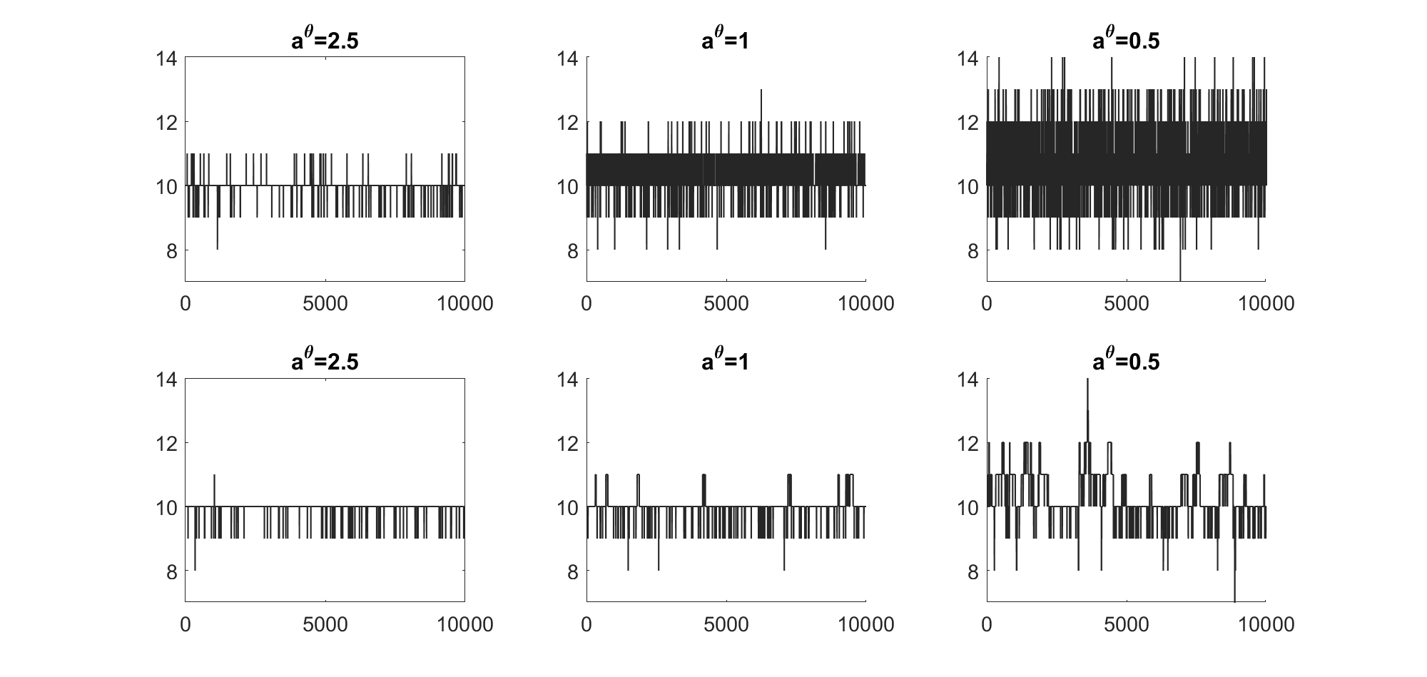
Figure 2: Data set simulated under the dense scenario with $(m,{H_{0}})=(50,10)$. 10,000 posterior draws of $H^{\star}$ using Algorithm 1 (top) and Algorithm 2 (bottom) for ESP priors with $a^{\theta}=2.5$ (left-hand side), $a^{\theta}=1$ (middle), $a^{\theta}=0.5$ (right-hand side), $c^{\theta}=2.5$ and $\alpha\sim\mathcal{G}(6,2)$.

For each of the 25 simulated data sets, we evaluate all 18 possible data scenarios and ESP priors through Monte Carlo estimates of following statistics: to assess the reliability of ${H}^{\star}$ as an estimator of the true number ${H_{0}}$ of factors, we consider the mode $\hat{H}^{\star}$ of the posterior distribution $p({H}^{\star}|{\mathbf{y}})$ and the magnitude of the posterior ordinate $p({H}^{\star}={H_{0}}|{\mathbf{y}})$. To assess the accuracy in estimating the true covariance matrix $\boldsymbol{\Omega}_{0}=\boldsymbol{\beta}_{0}\boldsymbol{\beta}_{0}^{\top}+\boldsymbol{\Sigma}_{0}$ of the data through the covariance matrix $\boldsymbol{\Omega}=\boldsymbol{\beta}\boldsymbol{\beta}^{\top}+\boldsymbol{\Sigma}$ implied by the overfitting model (23), we consider the mean squared error (MSE) defined by

$$\mbox{\rm MSE}_{\Omega}=\sum_{i}\sum_{\ell\leq i}\mathbb{E}(\left(\Omega_{i\ell}-\Omega_{0,i\ell}\right)^{2}|{\mathbf{y}})/(m(m+1)/2).$$

Table 1 reports, for all 18 possible data scenarios and ESP priors the median, the 5% as well as the 95% quantiles of these statistics across all 25 simulated data sets. Regarding the covariance matrix $\boldsymbol{\Omega}_{0}$, all three ESP priors exhibit more or less identical MSEs which increase with $H_{0}$ and are considerably smaller for sparse than for dense loading matrices. All three ESP priors are equally successful in recovering ${H_{0}}$ from the posterior mode $\hat{H}^{\star}$. Interestingly, we observe considerable variation in posterior concentration at the true value $H_{0}$ across the three values of $a^{\theta}$. The posterior ordinate $p({H}^{\star}={H_{0}}|{\mathbf{y}})$ is close to 1 for the F-mixture with $a^{\theta}=2.5$ in all six data scenarios, even for the sparse settings. For the other two choices of $a^{\theta}$, $p({H}^{\star}={H_{0}}|{\mathbf{y}})$ takes values considerably smaller than 1, in particular for the regularized horseshoe mixture.

As explained at the end of Section 5.1, the decreasing order statistics $\tau_{(1)}>\ldots>\tau_{(H)}$ of the unordered slab probabilities $\tau_{1},\ldots,\tau_{H}$ can be exploited to obtain the CUSP representation of the various ESP priors. To gain additional insights, detailed results are reported for a data set simulated under the dense scenario with $(m,{H_{0}})=(50,10)$. Figure 1 shows box plots of the posterior draws of the increasing spike probability $\pi_{h}=1-\tau_{(h)}$ as well as the corresponding column specific shrinkage parameter $\theta^{\star}_{h}$ in the CUSP representation for all three ESP priors. As a result of the implicit CUSP property of an ESP prior, the posterior of the spike probability $\pi_{h}$ is increasingly pulled towards one, while the posterior of $\theta^{\star}_{h}$ is pulled towards zero as $h$ increases. Under all three ESP priors, the information in the data induces a clear posterior gap between active and inactive columns at the true value $h={H_{0}}=10$.

Regarding MCMC performance, Algorithm 1 shows good mixing properties for all identified parameters. Without any thinning of the 10,000 posterior draws, the median effective sampling rate of, respectively, $\log|\boldsymbol{\Omega}|$ and $\|\boldsymbol{\Omega}^{-1}\|_{F}$ across all 25 simulated data sets is, on average, equal to 27.7% and 14.4%, yielding an average median effective sampling size (ESS) of 2768 and 1435. For further illustration, Figure 2 shows 10,000 posterior draws of $H^{\star}$ obtained by Algorithm 1 and Algorithm 2 for all three ESP priors for a single data set simulated under the dense scenario with $(m,{H_{0}})=(50,10)$. Obviously, Algorithm 1, which uses the F-mixture of $\theta_{h}$ for separating active from inactive columns, shows much better mixing than Algorithm 2, which exploits the marginalized $t$-mixture of the columns $\boldsymbol{\beta}_{h}$ of the loading matrix for this purpose.

The variation of the posterior draws of $H^{\star}$ in Figure 2 mirrors the concentration in the posterior distribution $p(H^{\star}|{\mathbf{y}})$. As discussed earlier, the posterior ordinate $p(H^{\star}=H_{0}=10|{\mathbf{y}})$ is considerably smaller than 1 for the regularized horseshoe mixture (see again Table 1). Under Algorithm 1, the corresponding posterior draws show excellent mixing over the discrete posterior $p(H^{\star}|{\mathbf{y}})$, which is the main motivation for Kowal and Canale (2022) to suggest this prior in the first place. However, this comes at the cost of less posterior concentration. For the regularized Lasso mixture, posterior concentration is more pronounced (see again Table 1). Nevertheless, the posterior draws show rapid movement across the posterior distribution $p(H^{\star}|{\mathbf{y}})$ under Algorithm 1. Algorithm 1 yields a highly concentrated posterior distribution $p(H^{\star}|{\mathbf{y}})$ under $a^{\theta}=2.5$ not only for this specific data set, but also for most others (see again Table 1).

A valid question raised by Kowal and Canale (2022) is whether such strong posterior concentration is the result of a badly mixing sampler. For the specific example in Figure 2, nearly perfect posterior concentration under $a^{\theta}=2.5$ is confirmed by Algorithm 2. However, among the 450 simulated data sets we found many cases, in particular for $a^{\theta}=1$ and $a^{\theta}=0.5$, where Algorithm 2 quickly moved from the initial model with three active columns to the true value of $H_{0}$, only then to get stuck at $H_{0}$ and produce overly optimistic posterior concentration compared to Algorithm 1 (which was mixing well also in these cases).

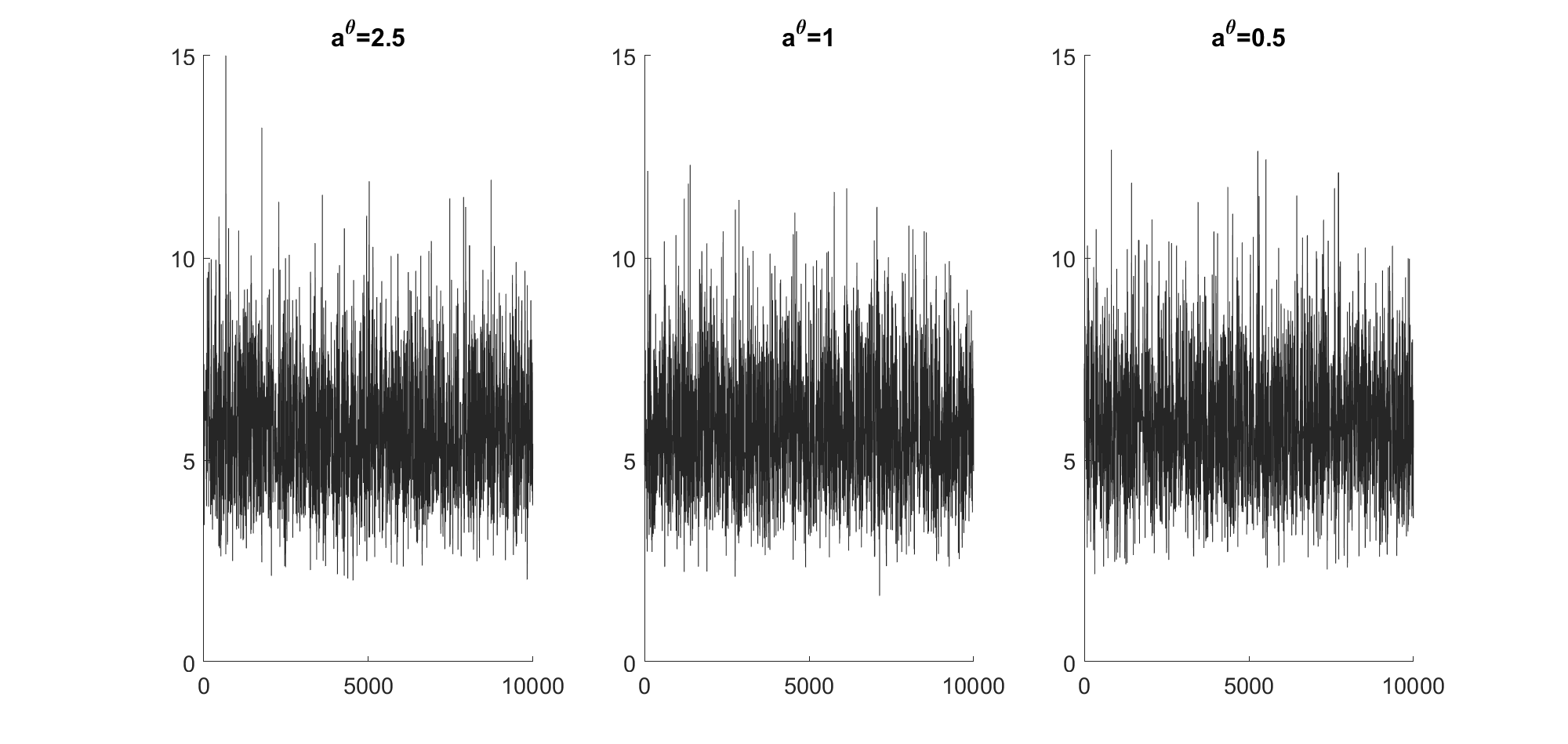
Figure 3: Data set simulated under the dense scenario with $(m,{H_{0}})=(50,10)$. 10,000 posterior draws of $\alpha$ for ESP priors with $a^{\theta}=2.5$ (left-hand side), $a^{\theta}=1$ (middle), $a^{\theta}=0.5$ (right-hand side), $c^{\theta}=2.5$ and $\alpha\sim\mathcal{G}(6,2)$.

Finally, Figure 3 shows posterior draws of the strength parameter of the 1BP prior, $\alpha$, for all three choices of $a^{\theta}$ in the spike-and-slab prior on $\theta_{h}$ for the dense scenario with $(m,{H_{0}})=(50,10)$. Posterior inference w.r.t. $\alpha$ is rather robust regarding the choice of $a^{\theta}$ and strongly supports values of $\alpha$ considerably smaller than $H=24$.

Comparison to other priors.

Choosing $\alpha=H$ corresponds to the uniform prior $\tau_{h}\sim\mathcal{U}\left[0,1\right]$ applied in Zhao et al. (2016) and a simplified version of Algorithm 1 with $\alpha=H$ fixed can be used for posterior inference under this prior. Table 2 shows, for all 9 combinations of sparse data scenarios and choices of the hyperparameter $a^{\theta}$ in the spike-and-slab prior on $\theta_{h}$, how the various statistics change under this prior. Interestingly, whether the data are informative enough to overrule the strong impact of the uniform prior on the prior distribution of the spike probabilities (which are pulled away from one, see again Section 4.4) depends on the chosen specification for the spike-and-slab prior. Under the F-mixture prior with $a^{\theta}=2.5$ and under the regularized Lasso mixture prior, we still manage to retrieve the true number of factors, however with less posterior concentration than before. On the other hand, the true number of factors is systematically overfitted under the regularized horseshoe mixture prior, in particular for the two larger models.

Table 2: Performance of the spike-and-slab prior (25) with $a^{\theta}=2.5$ (F), $a^{\theta}=1$ (L), $a^{\theta}=0.5$ (H), and $c^{\theta}=2.5$ under the uniform prior $\tau_{h}\sim\mathcal{U}\left[0,1\right]$ for the three sparse data scenarios. The columns M and Q show the median, the 5% and the 95% quantile of the various statistics over the simulated data sets.

		$\hat{H}^{\star}$		$p({H}^{\star}={H_{0}}|{\mathbf{y}})$		$\mbox{\rm MSE}_{\Omega}$
$(m,{H_{0}})$	Prior	M	Q	M	Q	M	Q
(20,5)	F	5	(5,5)	0.91	(0.57,0.97)	0.48	(0.31,0.96)
	L	5	(5,5)	0.68	(0.28,0.78)	0.42	(0.28,0.68)
	H	5	(5,6)	0.41	(0.32,0.51)	0.52	(0.21,0.89)
(50,10)	F	10	(10,10)	0.96	(0.89,0.98)	1.14	(0.90,1.58)
	L	10	(10,10)	0.53	(0.45,0.61)	1.21	(0.89,1.65)
	H	12	(11,12)	0.13	(0.08,0.16)	1.27	(0.99,1.87)
(100,15)	F	15	(15,15)	0.98	(0.98,0.99)	1.97	(1.69,2.61)
	L	15	(15,15)	0.62	(0.56,0.67)	2.10	(1.64,2.47)
	H	17	(16,17)	0.13	(0.10,0.16)	2.00	(1.68,2.41)

In addition, to compare finite ESP priors to the original CUSP prior, we reproduce some of the performance measures reported in Table 1 of Legramanti et al. (2020) for dense factor models in Table 1. The statistical performance of all finite ESP prior is identical with the CUSP prior regarding inference on $H^{\star}$ and very similar regarding $\mbox{\rm MSE}_{\Omega}$. However, run times improve considerably under a finite ESP prior, due to the gain in sampling the binary indicators $S_{1},\ldots,S_{H}$ instead of the categorical indicators $z_{1},\ldots,z_{H}$. Furthermore, for the two statistics of $\boldsymbol{\Omega}$ described above, we achieve higher effective sampling sizes than Legramanti et al. (2020) where the median of the ESS of 2,000 thinned draws is on average equal to 368 for a slightly different statistic of $\boldsymbol{\Omega}$. This increased sampling efficiency results from partial marginalization in Algorithm 1, where we sample the strength parameter $\alpha$ and the indicators $S_{1},\ldots,S_{H}$ without conditioning on the slab probabilities $\tau_{1},\ldots,\tau_{H}$, see again Section 4.1.

6 Conclusion

In the present paper, we discuss shrinkage priors that automatically impose increasing shrinkage on a sequence of parameters. Our main motivation came from Bayesian factor analysis, where increasing shrinkage is imposed on the loading matrix as the column index increases to allow statistical inference with respect to the unknown factor dimension.

We briefly reviewed the CUSP prior of Legramanti et al. (2020), which is a spike-and-slab prior, where the spike probability is stochastically increasing and constructed from the stick-breaking representation of a DP prior. As a first contribution, this prior is extended to a generalized CUSP prior involving arbitrary stick-breaking representations. This prior subsumes several priors introduced earlier in the literature, involving various stick-breaking representations based on beta distributions Ročková and George (2017); Heaukulani and Roy (2020); Ohn and Kim (2022); Frühwirth-Schnatter et al. (2022b); Kowal and Canale (2022). As a second contribution, we prove that exchangeable spike-and-slab shrinkage (ESP) priors, which are popular and widely used in many areas of applied Bayesian inference, can be represented as a finite generalized CUSP prior. The CUSP representation can be easily derived from the decreasing order statistics of the slab probabilities.

Working with an ESP prior on a sequence of parameters which is invariant to the ordering and, at the same time, implicitly imposes increasing shrinkage without forcing explicit order constraints on the slab probabilities is very convenient. It allows, in particular, to design efficient MCMC samplers under the ESP prior and to derive the CUSP representation during post-processing. As opposed to this, direct sampling under the order constraints in the CUSP representation is more challenging and often a truncated CUSP prior with $H<\infty$ has to be employed for infinite models. Using instead an ESP prior with large $H$ with the same spike-and-slab distribution for the parameter $\theta_{h}$ as the infinite CUSP prior will induce similar increasing shrinkage, while classification is much simplified and reduces to sampling $H$ binary indicators instead of $H$ categorical variables with $H$ categories.

An application to sparse Bayesian factor analysis illustrates the usefulness of the findings of this paper. A new exchangeable spike-and-slab shrinkage prior based on the triple gamma prior Cadonna et al. (2020) is introduced. In the context of Bayesian factor analysis, this ESP prior induces increasing shrinkage in the columns of the loading matrix. In a simulation study it is shown that this prior is helpful for estimating the unknown number of factors. The main focus of this application to sparse Bayesian factor analysis lies on column sparsity, but as mentioned in the introduction, element-wise sparsity is another common goal in factor analysis. Combining both approaches is an interesting venue for further research and is investigated in Frühwirth-Schnatter et al. (2022b).

Appendix

We prove that the finite 1PB prior (14) has a representation as a finite CUSP prior as in (5) and (6), where the sticks $\nu_{h}$, $h=1,\ldots,H$ are an independent sequence of beta random variables,

$$\nu_{h}\sim\mathcal{B}\left(1,\alpha\frac{H-h+1}{H}\right).$$ (36)

Equivalently, the decreasing slab probabilities can be represented as:

$$\tau_{(h)}=1-\pi_{h}=\prod_{\ell=1}^{h}(1-\nu_{\ell})=\prod_{\ell=1}^{h}\nu^{\star}_{\ell}=\tau_{(h-1)}\nu^{\star}_{h},$$ (37)

where $\nu^{\star}_{h}\,\,i.i.d.\,\,\mathcal{B}\left(\alpha\frac{H-h+1}{H},1\right)$. It is easy to show that $\mathbb{E}(\pi_{h})$ satisfies following recursion for all $h$. From (37) we obtain

$$\mathbb{E}(\tau_{(h)})=\mathbb{E}(\tau_{(h-1)})\mathbb{E}(\nu^{\star}_{h})=\mathbb{E}(\tau_{(h-1)})C_{h},\qquad C_{h}=\frac{\alpha(1-\frac{h-1}{H})}{\alpha(1-\frac{h-1}{H})+1}<1.$$

Hence, $\mathbb{E}(\tau_{(h)})$ is a decreasing sequence and, consequently, $\mathbb{E}(\pi_{h})=1-\mathbb{E}(\tau_{(h)})$ is increasing. It follows immediately that prior (14) converges to the CUSP prior proposed by Legramanti et al. (2020) with strength parameter $\alpha$ as $H$ goes to infinity, since $\lim_{H\rightarrow\infty}\frac{H-h+1}{H}=1$. To prove (36) and (37), we follow Teh et al. (2007) and take a closer look at the distribution of the decreasing order statistics $\tau_{(1)}>\ldots>\tau_{(H)}$. The unordered slab probabilities $\tau_{h}$ in (14) exhibit, respectively, following pdf and cdf:

$$p(\tau_{h})=\frac{\alpha}{H}\tau_{h}^{\frac{\alpha}{H}-1},\quad F_{\tau_{h}}(\tau)={\rm P}(\tau_{h}\leq\tau)=\tau^{\frac{\alpha}{H}}.$$

Let $T$ be an arbitrary natural number. First we show that for any sequence of $T$ iid r.v. $X_{h}\sim\mathcal{B}\left(\frac{\alpha}{H},1\right)$, the maximum $X_{\mbox{{\rm\tiny max}}}=\max(X_{1},\ldots,X_{T})$ follows the $\mathcal{B}\left(\frac{T\alpha}{H},1\right)$-distribution:

$$F_{X_{\max}}(x)=\prod_{h=1}^{T}{\rm P}(X_{h}\leq x)=(x^{\frac{\alpha}{H}})^{T}=x^{\frac{T\alpha}{H}}.$$ (38)

With $T=H$, it follows from (38) that under prior (14) the largest order statistic, $\tau_{(1)}=\max(\tau_{1},\ldots,\tau_{H})$ follows $\tau_{(1)}\sim\mathcal{B}\left(\alpha,1\right)$. Given the order statistic $\tau_{(1)},\ldots,\tau_{(h-1)}$, the range the remaining unordered slab probabilities $\tau_{h}|(\tau_{h}<\tau_{(h-1)})$ is obviously restricted to $[0,\tau_{(h-1)}]$ and the corresponding cdf is given by:

$$F_{\tau_{h}}(\tau)={\rm P}(\tau_{h}\leq\tau|\tau_{h}<\tau_{(h-1)})=\frac{\int_{0}^{\tau}\frac{\alpha}{H}\tau_{h}^{\frac{\alpha}{H}-1}\,d\,\tau_{h}}{\int_{0}^{\tau_{(h-1)}}\frac{\alpha}{H}\tau_{h}^{\frac{\alpha}{H}-1}\,d\,\tau_{h}}=\frac{\tau^{\frac{\alpha}{H}}}{(\tau_{(h-1)})^{\frac{\alpha}{H}}}=\left(\frac{\tau}{\tau_{(h-1)}}\right)^{\frac{\alpha}{H}}.$$

Hence, all $H-h+1$ slab probabilities $\tau_{h}$ smaller than $\tau_{(h-1)}$ are independent and can be presented as $\tau_{h}=X_{h}\tau_{(h-1)}$, were $X_{h}\sim\mathcal{B}\left(\frac{\alpha}{H},1\right)$. This follows immediately from

$$F_{X_{h}}(x)={\rm P}(X_{h}\leq x)={\rm P}(\tau_{h}\leq x\tau_{(h-1)})=\left(\frac{x\tau_{(h-1)}}{\tau_{(h-1)}}\right)^{\frac{\alpha}{H}}=x^{\frac{\alpha}{H}}.$$

Given the order statistic $\tau_{(h-1)}$, the order statistic $\tau_{(h)}$ can be derived as $\tau_{(h)}=\tau_{(h-1)}\nu_{h}^{\star}$, where $\nu_{h}^{\star}=\max_{\ell:\tau_{\ell}<\tau_{(h-1)}}X_{h}$. Using (38) with $T=H-h+1$, we obtain:

$$\tau_{(h)}=\tau_{(h-1)}\nu_{h}^{\star},\qquad\nu_{h}^{\star}\sim\mathcal{B}\left(\alpha\frac{H-h+1}{H},1\right).$$

From this, it follows immediately that the ordered spike probabilities $\pi_{h}=1-\tau_{(h)}$ and the ordered slab probabilities $\pi_{h}^{\star}=\tau_{(h)}$ can be represented as, respectively, in (36) and (37).

References

- Anderson and Rubin (1956) Anderson, T. W. and H. Rubin (1956). Statistical inference in factor analysis. In Proceedings of the Third Berkeley Symposium on Mathematical Statistics and Probability, Volume V, pp. 111–150.
- Avalos-Pacheco et al. (2022) Avalos-Pacheco, A., D. Rossell, and R. S. Savage (2022). Heterogeneous large datasets integration using Bayesian latent factor regression. Bayesian Analysis 17, 33–66.
- Bhattacharya and Dunson (2011) Bhattacharya, A. and D. Dunson (2011). Sparse Bayesian infinite factor models. Biometrika 98, 291–306.
- Cadonna et al. (2020) Cadonna, A., S. Frühwirth-Schnatter, and P. Knaus (2020). Triple the gamma – A unifying shrinkage prior for variance and variable selection in sparse state space and TVP models. Econometrics 8, 20.
- Carvalho et al. (2008) Carvalho, C. M., J. Chang, J. E. Lucas, J. Nevins, Q. Wang, and M. West (2008). High-dimensional sparse factor modeling: Applications in gene expression genomics. Journal of the American Statistical Association 103, 1438–1456.
- Conti et al. (2014) Conti, G., S. Frühwirth-Schnatter, J. J. Heckman, and R. Piatek (2014). Bayesian exploratory factor analysis. Journal of Econometrics 183, 31–57.
- De Vito et al. (2021) De Vito, R., R. Bellio, L. Trippa, and G. Parmigiani (2021). Bayesian multi-study factor analysis for high-throughput biological data. The Annals of Applied Statistics 15, 1723 – 1741.
- Durante (2017) Durante, D. (2017). A note on the multiplicative gamma process. Statistics and Probability Letters 122, 198–204.
- Frühwirth-Schnatter et al. (2022a) Frühwirth-Schnatter, S., D. Hosszejni, and H. Lopes (2022a). When is counts - Econometric identification of factor models based on GLT structures. ArXiv 2301.06354.
- Frühwirth-Schnatter et al. (2022b) Frühwirth-Schnatter, S., D. Hosszejni, and H. F. Lopes (2022b). Sparse finite Bayesian factor analysis when the number of factors is unknown. ArXiv 2301.06459.
- Frühwirth-Schnatter and Lopes (2010) Frühwirth-Schnatter, S. and H. Lopes (2010). Parsimonious Bayesian Factor Analysis when the Number of Factors is Unknown. Research report, Booth School of Business, University of Chicago.
- Ghahramani et al. (2007) Ghahramani, Z., T. L. Griffiths, and P. Sollich (2007). Bayesian nonparametric latent feature models (with discussion and rejoinder). In J. M. Bernardo, M. J. Bayarri, J. O. Berger, A. P. Dawid, D. Heckerman, A. F. M. Smith, and M. West (Eds.), Bayesian Statistics 8, pp. 1–25. Oxford: Oxford University Press.
- Heaukulani and Roy (2020) Heaukulani, C. and D. M. Roy (2020). Gibbs-type Indian Buffet Processes. Bayesian Analysis 15, 683–710.
- Hosszejni and Frühwirth-Schnatter (2022) Hosszejni, D. and S. Frühwirth-Schnatter (2022). Cover it up! Bipartite graphs uncover identifiability in sparse factor analysis. arXiv 2211.00671.
- Kastner (2019) Kastner, G. (2019). Sparse Bayesian time-varying covariance estimation in many dimensions. Journal of Econometrics 210, 98–115.
- Kaufmann and Schuhmacher (2019) Kaufmann, S. and C. Schuhmacher (2019). Bayesian estimation of sparse dynamic factor models with order-independent and ex-post identification. Journal of Econometrics 210, 116–134.
- Kowal and Canale (2022) Kowal, D. R. and A. Canale (2022). Semiparametric functional factor models with Bayesian rank selection. arXiv 2108.02151.
- Legramanti et al. (2020) Legramanti, S., D. Durante, and D. B. Dunson (2020). Bayesian cumulative shrinkage for infinite factorizations. Biometrika 107, 745–752.
- Murphy et al. (2020) Murphy, K., C. Viroli, and I. C. Gormley (2020). Infinite mixtures of infinite factor analysers. Bayesian Analyis 15, 937–963.
- Ohn and Kim (2022) Ohn, I. and Y. Kim (2022). Posterior Consistency of Factor Dimensionality in High-Dimensional Sparse Factor Models. Bayesian Analysis 17, 491–514.
- Ročková and George (2017) Ročková, V. and E. I. George (2017). Fast Bayesian factor analysis via automatic rotation to sparsity. Journal of the American Statistical Association 111, 1608–1622.
- Schiavon and Canale (2020) Schiavon, L. and A. Canale (2020). On the truncation criteria in infinite factor models. Stat 9, e298.
- Schiavon et al. (2021) Schiavon, L., A. Canale, and D. B. Dunson (2021). Generalized infinite factorization models. arXiv 2103.10333.
- Sethuraman (1994) Sethuraman, J. (1994). A constructive definition of Dirichlet priors. Statistica Sinica 4, 639–650.
- Teh et al. (2007) Teh, Y. W., D. Görür, and Z. Ghahramani (2007). Stick-breaking construction for the Indian buffet process. In M. Meila and X. Shen (Eds.), Proceedings of the Eleventh International Conference on Artificial Intelligence and Statistics, Volume 2 of Proceedings of Machine Learning Research, San Juan, Puerto Rico, pp. 556–563.
- West (2003) West, M. (2003). Bayesian factor regression models in the “large p, small n” paradigm. In J. M. Bernardo, M. J. Bayarri, J. O. Berger, A. P. Dawid, D. Heckerman, A. F. M. Smith, and M. West (Eds.), Bayesian Statistics 7, pp. 733–742. Oxford: Oxford University Press.
- Zhao et al. (2016) Zhao, S., C. Gao, S. Mukherjee, and B. E. Engelhardt (2016). Bayesian group factor analysis with structured sparsity. Journal of Machine Learning Research 17, 1–47.