Pressure anisotropy and viscous heating in weakly collisional plasma turbulence

Abstract

Pressure anisotropy can strongly influence the dynamics of weakly collisional, high-beta plasmas, but its effects are missed by standard magnetohydrodynamics (MHD). Small changes to the magnetic-field strength generate large pressure-anisotropy forces, heating the plasma, driving instabilities, and rearranging flows, even on scales far above the particles’ gyroscales where kinetic effects are traditionally considered most important. Here, we study the influence of pressure anisotropy on turbulent plasmas threaded by a mean magnetic field (Alfvénic turbulence). Extending previous results that were concerned with Braginskii MHD, we consider a wide range of regimes and parameters using a simplified fluid model based on drift kinetics with heat fluxes calculated using a Landau-fluid closure. We show that viscous (pressure-anisotropy) heating dissipates between a quarter (in collisionless regimes) and half (in collisional regimes) of the turbulent cascade power injected at large scales; this does not depend strongly on either plasma beta or the ion-to-electron temperature ratio. This will in turn influence the plasma’s thermodynamics by regulating energy partition between different dissipation channels (e.g., electron and ion heat). Due to the pressure anisotropy’s rapid dynamical feedback onto the flows that create it – an effect we term ‘magneto-immutability’ – the viscous heating is confined to a narrow range of scales near the forcing scale, supporting a nearly conservative, MHD-like inertial-range cascade, via which the rest of the energy is transferred to small scales. Despite the simplified model, our results – including the viscous heating rate, distributions, and turbulent spectra – compare favourably to recent hybrid-kinetic simulations. This is promising for the more general use of extended-fluid (or even MHD) approaches to model weakly collisional plasmas such as the intracluster medium, hot accretion flows, and the solar wind.

1 Introduction

Many hot, diffuse plasmas in astrophysical environments are weakly collisional, with Coulomb mean free paths that are comparable to relevant macroscopic scales in the system. Canonical examples include the intracluster medium in galaxy clusters (e.g., Fabian, 1994; Peterson & Fabian, 2006; Kunz et al., 2022), hot accretion flows such as those observed by the Event Horizon Telescope (Quataert, 2001; EHT Collaboration et al., 2019), the hotter phases of the interstellar and circumgalactic media (Cox, 2005; Tumlinson et al., 2017), and the solar wind and magnetosphere (Borovsky & Valdivia, 2018; Marsch, 2006). In all of these examples, the plasma is extremely well magnetised, in that the system scales are much larger than the ion gyroradius $\rho_{i}$. Coupled with the plasmas’ large Coulomb mean free paths, this implies that magnetic fields are crucial in providing the plasma with an internal cohesion that allows it to behave more or less like a collisional fluid (Kulsrud, 1983). However, despite the particle motion’s allegiance to the local magnetic field, in many environments the magnetic fields are energetically subdominant as measured by $\beta=8\pi p/B^{2}$, where $p$ is a thermal pressure and $B^{2}/8\pi$ is the magnetic energy density. Under such conditions, small relative changes to the magnetic field can easily cause particle distributions to become unstable, suggesting that non-equilibrium kinetic physics should play a key role in the dynamics.

Nonetheless, such conditions are commonly modelled using collisional magnetohydrodynamics (MHD), usually for reasons of expediency, though with rigorous justification in some circumstances (e.g., Kulsrud, 1983; Schekochihin et al., 2009; Kunz et al., 2015). It is the first purpose of this article to explain why this is usually not appropriate, as a result of the aforementioned kinetic physics; it is the second purpose to explain why, in the end, it is not so bad after all. The physics we explore is that of pressure anisotropy (equivalently, temperature anisotropy), which is the difference between the thermal pressures in the directions perpendicular and parallel to the local magnetic field. The relevance of pressure anisotropy stems from it being the only non-isotropic piece of the pressure tensor that can survive on scales arbitrarily far above the particles’ gyroradii (Braginskii, 1965), making it a key physical ingredient in the momentum balance of weakly collisional plasmas (compared to collisional MHD; Chew et al., 1956; Kulsrud, 1983). At $\beta\gg 1$, a very small relative pressure anisotropy can lead to large bulk forces on the plasma. Furthermore, whenever the magnetic-field strength $B$ changes in time, $\Delta p$ is generated as a result of the conservation of single-particle adiabatic invariants. Put together, these two properties suggest that pressure-anisotropy stresses can vastly overwhelm the forces from the magnetic field or Reynolds stress in many high-$\beta$ environments.

Our study focuses on the role of pressure anisotropy in turbulence, specifically, in turbulence of the ‘Alfvénic’ variety that occurs when the system is threaded by a large-scale mean magnetic field. A particularly important example of such a system is the solar wind, which is our best natural laboratory for the study of Alfvénic turbulence under weakly collisional conditions. Such turbulence may also be relevant quasi-universally at smaller scales in systems without a mean magnetic field (Brandenburg & Subramanian, 2005; Schekochihin, 2022). We explore the structure and dynamics of weakly collisional Alfvénic turbulence, with a particular focus on their comparison with MHD and the implications for turbulent plasma heating. Pressure anisotropy provides another channel – effectively a viscosity – for damping injected mechanical energy into heat near the outer scales (e.g., Kunz et al., 2010; Yang et al., 2017). (Although this energy transfer can be reversible in some regimes, we will often refer to it as ‘viscous heating’ because at higher collisionalities the pressure-anisotropy stress increasingly resembles a parallel viscosity, with an associated heating rate that is positive definitive.) Because the pressure-anisotropy stress can easily overwhelm the magnetic tension and Reynolds stress in the high-$\beta$ limit (Squire et al., 2016), simple estimates suggest that this viscous heating should completely dominate over other heating mechanisms. However, we show that, because of the dynamical feedback of the pressure anisotropy on the plasma flow, such heating is confined to a narrow range of scales near the forcing scales, with a sizeable fraction (typically, the majority) of the energy making it through to participate in a nearly conservative turbulent cascade. This phenomenon, which was termed ‘magneto-immutability’ by Squire et al. (2019) (hereafter S+19) who studied the effect in the context of the simplified ‘Braginskii MHD’ model (see also Kempski et al. 2019; St-Onge et al. 2020), involves the force from the pressure anisotropy acting to rearrange the turbulence in order to reduce the influence of itself. This rearrangement constrains the global variation of $B$, hence the term ‘magneto-immutability’ to describe the effect. Its physics is analogous to that of incompressibility, in which the pressure force that results from a fluid compression rapidly drives a flow that counters the compression, thereby eliminating such motions and minimising variations in the density. This explains our flippant declaration above about the article’s purpose: simple estimates suggest pressure anisotropy should dominate the force balance and heating, modifying the dynamics compared to MHD; but, the effect of this modification is to minimise the pressure anisotropy’s own influence, thus allowing turbulent dynamics that look broadly similar to MHD below the outer scales (albeit with a few important differences).

These ideas complicate the already complex story of turbulent heating in weakly collisional plasmas (e.g., Quataert & Gruzinov, 1999; Kunz et al., 2010; Howes, 2010; Kawazura et al., 2020; Meyrand et al., 2021; Yang et al., 2022; Arzamasskiy et al., 2023). A useful concept is the ‘cascade efficiency’: the fraction of energy available to cascade down to small scales and heat the plasma via different collisionless mechanisms (Schekochihin et al., 2009; Chandran et al., 2010; Arzamasskiy et al., 2019). In our simulations, between ${\simeq}20\%$ and ${\simeq}45\%$ of the energy is lost through pressure-anisotropy heating at large scales (giving a cascade efficiency of ${\gtrsim}55\%$ for our choice of large-scale forcing), independently of $\beta$ and the electron-to-ion temperature ratio. Magneto-immutability ensures that the remainder of the energy cascades nearly conservatively, presumably eventually heating at small scales in the way predicted by gyrokinetics (Howes et al., 2008; Schekochihin et al., 2009; Kunz et al., 2018). With different heating processes implying a different partition of turbulent energy between electron and ion heat, or between perpendicular and parallel heat, these apparently esoteric details of the turbulent structure can strongly influence the basic thermodynamics of the plasma. For instance, while it is well known that small-scale collisionless processes in high-$\beta$ plasmas generically heat ions more than electrons (Howes, 2010; Parashar et al., 2018; Kawazura et al., 2020; Roy et al., 2022), large-scale pressure anisotropy can also heat collisionless electrons (Sharma et al., 2007), meaning that the cascade efficiency – and thus magneto-immutability – could directly control the ion-to-electron heating ratio. While we do not explicitly study electron physics, our study provides a useful foundation for distilling and quantifying the important physics, particularly through the idea that pressure-anisotropy heating is confined to a small range of large scales.

Our approach to the study of pressure anisotropy here is computational and simplified. We use the so-called CGL-Landau-fluid (hereafter CGL-LF) model (Chew et al., 1956; Snyder et al., 1997), which attempts to approximate collisionless heat fluxes in order to obtain a closed, simplified fluid model for plasma dynamics on scales well above $\rho_{i}$. This model, which is implemented using new numerical methods into the Athena++ framework (White et al., 2016; Stone et al., 2020), is then used to explore a range of conditions as the key parameters of the problem are varied. Detailed comparisons to otherwise equivalent MHD simulations are used to diagnose the influence of the pressure anisotropy on the turbulence and heating. A downside of the simplified-fluid-model approach is that various ad-hoc, loosely justified approximations are necessary. These approximations include those made to derive the fluid closure and its numerical realisation, and perhaps more importantly, the methods used to cope with the fast-growing $\rho_{i}$-scale firehose and mirror instabilities that will inevitably arise in real systems (Schekochihin et al., 2005; Bale et al., 2009; Kunz et al., 2014), but which cannot be captured correctly by drift kinetics (e.g., Rosin et al., 2011; Rincon et al., 2015). The upside of the approach, by contrast, is that the model effectively assumes infinite scale separation between the outer scale and $\rho_{i}$, which is clearly not possible in kinetic models that explicitly resolve $\rho_{i}$, but is the appropriate limit for most astrophysical systems. With this in mind, a useful subsidiary purpose of the article is to assess the successes of this simplified model in reproducing the physics seen in the hybrid-kinetic simulations of Arzamasskiy et al. (2023) (hereafter A+22), which explicitly resolve $\rho_{i}$ and the associated chaos of kinetic-scale instabilities at the expense of a much reduced inertial range. We find relatively good agreement in general, despite the ad-hoc nature of the fluid model and the interpretative difficulties associated with limited scale separation in the hybrid-kinetic simulations. In particular, we find similar cascade efficiencies (with a similar forcing scheme) and similar pressure-anisotropy distributions compared to A+22, with some caveats. Accordingly, the results of this work are quite promising for the use of CGL-LF approaches in modelling weakly collisional plasmas.

1.1 Outline

Although most of the basic theoretical concepts presented here have appeared in previous literature, we feel it is helpful to keep the majority of the discussion and notation self-contained to clarify the approximations and key concepts. Thus, §​ 2 presents an overview of the physics of pressure anisotropy and magneto-immutability, starting from the drift-kinetic model of Kulsrud (1983). Lacking any quantitative theory of the important effects, we focus on qualitative explanations for the behaviour and effect of the pressure anisotropy and heat fluxes in different regimes. We also define the ‘interruption number’ $\mathcal{I}$, which quantifies the expected strength of pressure-anisotropic effects in Alfvénic turbulence, analogously to the Reynolds number or Mach number in fluids. In §​ 3 we then outline the numerical methods and diagnostics, before presenting detailed simulation results in §​ 4. Leveraging the versatility of the simplified fluid model, a focus of the results is the direct comparison to ‘passive-$\Delta p$’ simulations. These are identical to the standard simulations but with the anisotropic pressure force artificially removed, thereby affording a direct comparison to a counterfactual situation where magneto-immutability does not exist. The comparison clearly demonstrates both the similarities and differences between our pressure-anisotropic Landau-fluid model and MHD in spectra, distributions, and scale-dependent heating functions. We follow with discussions of the key uncertainties related to kinetic instabilities (§​ 5.1) and of the distinction between magneto-immutability and the so-called ‘spherically polarised’ states measured in the solar wind (a complicating factor for interpreting spacecraft observations). We also summarise most salient differences between magneto-immutable and MHD turbulence (§​ 5.2). A full list of the simulations with their important parameters is given in table 1. We conclude in §​ 6. An appendix presents various technical results related to the numerical finite-volume implementation in the Athena++ code (White et al., 2016; Stone et al., 2020), including linear-wave convergence tests and a new Riemann solver for the CGL system (albeit one that we ultimately did not use in the simulations).

2 Theoretical and phenomenological background

2.1 The evolution and effect of pressure anisotropy

In this section, we introduce the basic concepts necessary to understand the numerical results presented in §4. The goal is to provide some intuitive understanding of the effects of pressure anisotropy in different plasma regimes, starting from the basic equations for a collisionless plasma on large scales. We begin by assuming that the plasma pressure tensor is gyrotropic but anisotropic – it is invariant under rotations about the magnetic field, but can differ in the directions perpendicular and parallel to the field. This is justified for ‘MHD-range’ scales, viz., those larger than the ion gyroscale in space and slower than the ion gyrofrequency in time. We also assume a single ion species and isothermal electrons, which allows us to drop the anisotropic component of the electron pressure and obtain single-fluid equations for the dynamics of the ions. Although this can be formally justified in the moderately collisional limit using the electron’s larger collision frequency and fast thermal speed (Rosin et al., 2011), here the choice is primarily one of simplicity, since we wish to focus on the dynamical effects of pressure anisotropy on fluid motions. Most of our simulations in this work will assume cold electrons anyway, in order to better understand and diagnose the basic processes at play.

With these assumptions, the first three moments of the ion distribution function satisfy (Chew et al., 1956; Kulsrud, 1983)

$$\partial_{t}\rho+\mbox{\boldmath{$\nabla$}}\,\mbox{\boldmath{$\cdot$}}\,(\rho\bm{u})=0,$$ (1)

$$\rho\left(\partial_{t}\bm{u}+\bm{u}\,\mbox{\boldmath{$\cdot$}}\,\mbox{\boldmath{$\nabla$}}\bm{u}\right)=-\mbox{\boldmath{$\nabla$}}\left(T_{e}\rho+p_{\perp}+\frac{B^{2}}{8\pi}\right)+\mbox{\boldmath{$\nabla$}}\,\mbox{\boldmath{$\cdot$}}\,\left[\hat{\bm{b}}\hat{\bm{b}}\left(\Delta p+\frac{B^{2}}{4\pi}\right)\right],$$ (2)

$$\partial_{t}\bm{B}=\mbox{\boldmath{$\nabla$}}\,\mbox{\boldmath{$\times$}}\,(\bm{u}\,\mbox{\boldmath{$\times$}}\,\bm{B}),$$ (3)

$$\partial_{t}p_{\perp}+\mbox{\boldmath{$\nabla$}}\,\mbox{\boldmath{$\cdot$}}\,(p_{\perp}\bm{u})+p_{\perp}\mbox{\boldmath{$\nabla$}}\,\mbox{\boldmath{$\cdot$}}\,\bm{u}+\mbox{\boldmath{$\nabla$}}\,\mbox{\boldmath{$\cdot$}}\,(q_{\perp}\hat{\bm{b}})+q_{\perp}\mbox{\boldmath{$\nabla$}}\,\mbox{\boldmath{$\cdot$}}\,\hat{\bm{b}}=p_{\perp}\hat{\bm{b}}\hat{\bm{b}}\,\mbox{\boldmath{$:$}}\,\mbox{\boldmath{$\nabla$}}\bm{u}-\frac{1}{3}\nu_{\rm c}\Delta p,$$ (4)

$$\partial_{t}p_{\parallel}+\mbox{\boldmath{$\nabla$}}\,\mbox{\boldmath{$\cdot$}}\,(p_{\parallel}\bm{u})+\mbox{\boldmath{$\nabla$}}\,\mbox{\boldmath{$\cdot$}}\,(q_{\parallel}\hat{\bm{b}})-2q_{\perp}\mbox{\boldmath{$\nabla$}}\,\mbox{\boldmath{$\cdot$}}\,\hat{\bm{b}}=-2p_{\parallel}\hat{\bm{b}}\hat{\bm{b}}\,\mbox{\boldmath{$:$}}\,\mbox{\boldmath{$\nabla$}}\bm{u}+\frac{2}{3}\nu_{\rm c}\Delta p.$$ (5)

We use Gaussian-CGS units, $\bm{B}$ and $\bm{u}$ are the magnetic field and ion flow velocity (also approximately equal to the electron flow velocity for scales well above the ion gyroscale), $B\doteq\left|\bm{B}\right|$ and $\hat{\bm{b}}=\bm{B}/B$ denote the magnetic-field strength and direction, $\rho$ is the mass density, $\nu_{\rm c}$ is the ion-ion collision frequency, $p_{\perp}$ and $p_{\parallel}$ are the components of the ion pressure tensor perpendicular and parallel to the magnetic field, and $q_{\perp}$ and $q_{\parallel}$ are fluxes of perpendicular and parallel ion heat in the direction parallel to the magnetic field. The electron temperature $T_{e}$ is constant in time and space, because electrons are assumed isothermal (their pressure is $p_{e}=T_{e}\rho/m_{i}$, related to the ion density by quasi-neutrality assuming a single-ion-species plasma, and we neglect ion-electron collisions). Equations (1)–(5) are solved numerically in the conservative form given in appendix A. Importantly, this avoids explicitly computing the parallel rate of strain $\hat{\bm{b}}\hat{\bm{b}}\,\mbox{\boldmath{$:$}}\,\mbox{\boldmath{$\nabla$}}\bm{u}$, which can introduce serious numerical errors in some situations (Sharma & Hammett, 2011; S+19). We also define the Alfvén speed $v_{\rm A}=B/\sqrt{4\pi\rho}$, the total pressure $p_{0}\doteq 2p_{\perp}/3+p_{\|}/3$, the parallel sound speed $c_{\rm s\|}\doteq\sqrt{p_{\|}/\rho}$, the plasma beta $\beta\doteq 8\pi p_{0}/B^{2}$ (similarly $\beta_{\|}\doteq 8\pi p_{\|}/B^{2}$), the pressure anisotropy $\Delta p\doteq p_{\perp}-p_{\|}$, the normalised pressure anisotropy $\Delta\doteq\Delta p/p_{0}$, and the ‘anisotropy parameter,’

$$\Uptheta\doteq 1+\frac{4\pi\Delta p}{B^{2}},$$ (6)

which measures the relative change in the propagation speed of linear Alfvén waves (viz., $v_{\rm A}$) due to the contribution from the pressure-anisotropy stress (see §​ 2.1.2).

In order to avoid solving a kinetic equation for the heat fluxes, we close 1–5 with the expressions

$$q_{\perp}=-\frac{2c_{\rm s\|}^{2}}{\sqrt{2\pi}c_{\rm s\|}|k_{\parallel}|+\nu_{\rm c}}\left[\rho\nabla_{\parallel}\left(\frac{p_{\perp}}{\rho}\right)-p_{\perp}\left(1-\frac{p_{\perp}}{p_{\parallel}}\right)\frac{\nabla_{\parallel}B}{B}\right],$$ (7)

$$q_{\parallel}=-\frac{8c_{\rm s\|}^{2}}{\sqrt{8\pi}c_{\rm s\|}|k_{\parallel}|+(3\pi-8)\nu_{\rm c}}\rho\nabla_{\parallel}\left(\frac{p_{\parallel}}{\rho}\right).$$ (8)

These forms, which are known as a ‘Landau-fluid’ closure, were devised by Snyder et al. (1997), in order to match the linear behaviour of the true kinetic system as closely as possible (Hammett & Perkins, 1990; see also Passot et al. 2012). The $k_{\|}$ and $\nabla_{\|}=\hat{\bm{b}}\,\mbox{\boldmath{$\cdot$}}\,\mbox{\boldmath{$\nabla$}}$ in 7–8 are the parallel wavenumber and gradient operator, respectively, with the non-local gradient-like operator $\nabla_{\|}/|k_{\|}|$ arising as a result of approximating the effects of collisionless damping within the fluid model (see §​ 3.1.1 for further discussion). We will use the form 7–8 both computationally and as a useful intuitive guide for understanding the physical effect of the heat fluxes.

2.1.1 Energy conservation

With $T_{e}=0$, equations 1–5 conserve the total energy $E_{K}+E_{M}+E_{\rm th}$, where

$$E_{K}\doteq\frac{1}{2}\int{\rm d}\bm{x}\,\rho|\bm{u}|^{2},\quad E_{M}\doteq\frac{1}{8\pi}\int{\rm d}\bm{x}\,|\bm{B}|^{2},\quad E_{\rm th}\doteq\int{\rm d}\bm{x}\,\left(p_{\perp}+\frac{p_{\|}}{2}\right).$$ (9)

The rate of change of the thermal energy is

$$\frac{{\rm d}E_{\rm th}}{{\rm d}t}=\int{\rm d}\bm{x}\,(-p_{\perp}\mbox{\boldmath{$\nabla$}}\,\mbox{\boldmath{$\cdot$}}\,\bm{u}+\Delta p\,\hat{\bm{b}}\hat{\bm{b}}\,\mbox{\boldmath{$:$}}\,\mbox{\boldmath{$\nabla$}}\bm{u})=\int{\rm d}\bm{x}\,\left(p_{\|}\frac{1}{\rho}\frac{{\rm d}\rho}{{\rm d}t}+\Delta p\frac{1}{B}\frac{{\rm d}B}{{\rm d}t}\right),$$ (10)

where ${\rm d}/{\rm d}t=\partial_{t}+\bm{u}\,\mbox{\boldmath{$\cdot$}}\,\mbox{\boldmath{$\nabla$}}$ is the Lagrangian derivative and we used the continuity and induction equations to derive the second expression (see 13). We see that a positive correlation between $\Delta p$ and ${\rm d}B/{\rm d}t$ drives net heating of the plasma. This is not necessarily guaranteed: in essence, the term is similar to the compressive term $p_{\|}{\rm d}\!\ln\rho/{\rm d}t$ and can mediate oscillatory transfer between mechanical and thermal energy through pressure anisotropy. However, when collisions dominate the evolution of $\Delta p$, its effect becomes that of a parallel viscosity and $\Delta p\,{\rm d}\!\ln B/{\rm d}t$ is guaranteed to be positive (see 16 and discussion below). For this reason, we will often refer to this term as ‘viscous heating,’ even in the collisionless regime where it is more general. Note that, because ion-ion scattering must conserve energy, collisions only indirectly influence the thermal-energy evolution by changing the correlation between $\Delta p$ and ${\rm d}B/{\rm d}t$.

The case with $T_{e}\neq 0$ is addressed in §​ A.1.

2.1.2 Wave behaviour

Equations 1–5 admit five types of linear wave solutions: shear Alfvén waves, two modified magnetosonic-like waves, and two types of non-propagating entropy modes. These are discussed in more detail in §​ A.1.2 (see also Hunana et al., 2019; Majeski et al., 2023), where we give the relevant ideal dispersion relations (computed from 1–5 with $q_{\perp}=q_{\|}=0$ and $\nu_{c}=0$) and use their nonideal properties as a test of the numerical solvers. Here, we simply note that heat fluxes and/or collisions strongly damp all modes except for Alfvén waves, which, so long as $4\pi\Delta p>-B^{2}$, propagate undamped with the modified speed

$${v}_{\rm A,eff}=\sqrt{1+\frac{4\pi\Delta p}{B^{2}}}v_{\rm A}=\sqrt{{\Uptheta}}\,v_{\rm A}.$$ (11)

Linear Alfvénic modes are undamped because they do not involve any perturbation of $B^{2}$, and, therefore, do not create any pressure anisotropy. We see that for $4\pi\Delta p<-B^{2}$, ${v}_{\rm A,eff}$ becomes imaginary, which is the fluid manifestation of the firehose instability.

2.1.3 The collisionless, weakly collisional, and Braginskii-MHD regimes

It is helpful to examine the equation for the evolution of the pressure anisotropy, which may be obtained from 4 and 5:

$$\frac{{\rm d}}{{\rm d}t}\Delta p= \left(p_{\perp}+2p_{\|}\right)\hat{\bm{b}}\hat{\bm{b}}\,\mbox{\boldmath{$:$}}\,\mbox{\boldmath{$\nabla$}}\bm{u}-\left(2p_{\perp}-p_{\|}\right)\mbox{\boldmath{$\nabla$}}\,\mbox{\boldmath{$\cdot$}}\,\bm{u}$$

$$-\left\{\mbox{\boldmath{$\nabla$}}\,\mbox{\boldmath{$\cdot$}}\,\bigl{[}(q_{\perp}-q_{\|})\hat{\bm{b}}\bigr{]}+3q_{\perp}\mbox{\boldmath{$\nabla$}}\,\mbox{\boldmath{$\cdot$}}\,\hat{\bm{b}}\right\}-\nu_{\rm c}\Delta p.$$ (12)

Each term on the right-hand side is grouped according to its physical effect, which we discuss in turn below.

Changing field strength–

The first term on the right-hand side of 12 captures the creation of pressure anisotropy through the parallel rate of strain $\hat{\bm{b}}\hat{\bm{b}}\,\mbox{\boldmath{$:$}}\,\mbox{\boldmath{$\nabla$}}\bm{u}$, which is related to changes in the magnetic field strength through

$$\frac{1}{B}\frac{{\rm d}B}{{\rm d}t}=\hat{\bm{b}}\hat{\bm{b}}\,\mbox{\boldmath{$:$}}\,\mbox{\boldmath{$\nabla$}}\bm{u}-\mbox{\boldmath{$\nabla$}}\,\mbox{\boldmath{$\cdot$}}\,\bm{u}$$ (13)

(this equation is obtained from 3 after dotting it with $\hat{\bm{b}}$ and rearranging). Due to conservation of the collisionless adiabatic invariants $p_{\perp}/\rho B$ and $p_{\|}B^{2}/\rho^{3}$, positive $\Delta p$ is created in regions of increasing field strength, while negative $\Delta p$ is created in regions of decreasing field strength.

Compressions–

The second term is similar to the first but relates to changes in the plasma density. It is less important here, because of our focus on high-$\beta$ plasmas with low compressibility.

Heat fluxes–

The third term involves the heat fluxes, which, although neglected in the so-called double-adiabatic model, are always large in the $\beta\gtrsim 1$ regime where $\Delta p$ has a dynamically important effect (e.g., Hunana et al., 2019). The effect of this term can be understood by examining the ‘Landau fluid’ form of the heat fluxes given in 7–8. When $\Delta p\ll p_{0}$ and the spatial variation of density and $\hat{\bm{b}}$ is small compared to that of the temperature, these take the approximate forms

$$-\mbox{\boldmath{$\nabla$}}\,\mbox{\boldmath{$\cdot$}}\,(q_{\perp}\hat{\bm{b}})\approx-\hat{\bm{b}}\,\mbox{\boldmath{$\cdot$}}\,\mbox{\boldmath{$\nabla$}}q_{\perp}\approx\sqrt{\frac{2}{\pi}}\nabla_{\|}\left[\frac{c_{\rm s\|}^{2}}{c_{\rm s\|}|k_{\|}|+a_{\perp}\nu_{\rm c}}\nabla_{\|}p_{\perp}\right],$$ (14)

$$-\mbox{\boldmath{$\nabla$}}\,\mbox{\boldmath{$\cdot$}}\,(q_{\|}\hat{\bm{b}})\approx-\hat{\bm{b}}\,\mbox{\boldmath{$\cdot$}}\,\mbox{\boldmath{$\nabla$}}q_{\|}\approx\sqrt{\frac{8}{\pi}}\nabla_{\|}\left[\frac{c_{\rm s\|}^{2}}{c_{\rm s\|}|k_{\|}|+a_{\|}\nu_{\rm c}}\nabla_{\|}p_{\|}\right],$$ (15)

where $a_{\perp}$ and $a_{\|}$ are order-unity numerical factors (see 7 and 8). We see that, broadly speaking, the heat fluxes act like a parallel diffusion operator on $p_{\perp}$ and $p_{\|}$ (albeit a nonlocal one if $c_{\rm s\|}|k_{\|}|\gtrsim\nu_{\rm c}$), thus reducing the spatial variation of $\Delta p$ along the magnetic field.

Collisions–

The final term in 12 reduces the pressure anisotropy due to collisions, and, if large enough, causes 1–5 to reduce to standard, adiabatic MHD.

From this discussion, we see that the first two terms on the right-hand side of 12 are responsible for creating a pressure anisotropy from the motions of the plasma. By comparing the relative sizes of the other terms – ${\rm d}\Delta p/{\rm d}t$, the heat fluxes, and the collisional term – one finds three regimes each with qualitatively different $\Delta p$ evolution. To distinguish these, it is helpful to consider $\Delta p$ structures of parallel scale $k_{\|}^{-1}$ and assume that $\nabla_{\|}p_{\perp}\sim\nabla_{\|}p_{\|}\sim\nabla_{\|}\Delta p$, viz., that the relative variation in $p_{\perp}$, $p_{\|}$ and $\Delta p$ is of similar magnitudes (but note that it is not true that $p_{\perp}\sim p_{\|}\sim\Delta p$ because the variation in $p_{\perp}$ and $p_{\|}$ is small compared to their mean). Assuming Alfvénic motions, the time derivative scales as ${\rm d}\Delta p/{\rm d}t\sim\omega_{\rm A}\Delta p$ where $\omega_{\rm A}=k_{\|}v_{\rm A}$ is the Alfvén frequency, the heat-flux term scales as $\sim\![(k_{\|}c_{\rm s})^{2}/(|k_{\|}|c_{\rm s}+\nu_{\rm c})]\Delta p\sim[\beta\omega_{\rm A}/(\beta^{1/2}+\nu_{\rm c}/\omega_{\rm A})]\Delta p$, and the collisional term is just $\nu_{\rm c}\Delta p$. Restricting our discussion to $\beta\gtrsim 1$, the three regimes are:

Collisionless, $\bm{\nu_{\rm c}\ll\omega_{\rm A}}$–

If $\nu_{\rm c}\ll\omega_{\rm A}$, the collisional term cannot compete with ${\rm d}\Delta p/{\rm d}t\sim\omega_{\rm A}\Delta p$ to reduce $|\Delta p|$ significantly and so can be neglected. Because $\nu_{\rm c}/\omega_{\rm A}\lesssim 1$, the heat flux term scales as $\sim\!\beta^{1/2}\omega_{\rm A}\Delta p$, implying that heat fluxes are always important in this regime, smoothing $\Delta p$ in space rapidly compared to the Alfvénic motions that drive it.

Weakly Collisional, $\bm{\omega_{\rm A}\ll\nu_{\rm c}\lesssim\beta^{1/2}\omega_{\rm A}}$–

For $\nu_{\rm c}\gtrsim\omega_{\rm A}$, we can neglect ${\rm d}\Delta p/{\rm d}t$ in the balance of terms because collisions isotropize the pressure faster than $\Delta p$ can be created. However, if $\nu_{\rm c}$ also satisfies $\nu_{\rm c}\lesssim\beta^{1/2}\omega_{\rm A}$, the heat fluxes remain collisionless: they retain a similar form to the collisionless regime and thus have a similar effect on the dynamics, scaling as $\sim\!\beta^{1/2}\omega_{\rm A}\Delta p$, which remains larger than the collisional draining of $\Delta p$ (unless the parallel scales self-adjust; see Squire et al. 2017a). This weakly collisional regime is thus a hybrid collisional–collisionless one: although motions in the plasma are slower than the collision timescales, heat fluxes remain strong and are governed by collisionless physics (Mikhailovskii & Tsypin, 1971).

Braginskii MHD, $\bm{\beta^{1/2}\omega_{\rm A}\ll\nu_{\rm c}}$–

Once $\nu_{\rm c}\gg\beta^{1/2}\omega_{\rm A}$, in addition to neglecting ${\rm d}\Delta p/{\rm d}t$ compared to $\nu_{\rm c}\Delta p$, we see that the heat fluxes take the collisional form, scaling as $\sim\!(\beta\omega_{\rm A}^{2}/\nu_{\rm c})\Delta p$. Further, unlike in the weakly collisional regime, the heat fluxes become subdominant to $\nu_{\rm c}\Delta p$, since $\nu_{\rm c}\gg\beta\omega_{\rm A}^{2}/\nu_{\rm c}$ for $\nu_{\rm c}\gg\beta^{1/2}\omega_{\rm A}$. Thus at the same point that the heat fluxes take their collisional form, they become subdominant overall. In this regime, assuming incompressibility and $\Delta p\ll p_{\perp}\sim p_{\|}$, equation 12 takes the simple form

$$\Delta p\approx\frac{3p_{0}}{\nu_{\rm c}}\hat{\bm{b}}\hat{\bm{b}}\,\mbox{\boldmath{$:$}}\,\mbox{\boldmath{$\nabla$}}\bm{u},$$ (16)

which, when inserted into 2, yields a parallel viscous stress. Given this is effectively the parallel viscosity of Braginskii (1965), we refer to this regime as ‘Braginskii MHD.’

In previous work (S+19), we explored the effect of pressure anisotropy in the Braginskii-MHD regime, because of the simplicity of its physics and computational implementation. However, when combined with the condition that the pressure anisotropy has a dynamically important influence on the turbulence, $\nu_{\rm c}/\omega_{\rm A}\lesssim\beta\,\delta B_{\perp}^{2}/B_{0}^{2}$ (see §​ 2.2), the constraint $\nu_{\rm c}/\omega_{\rm A}\gg\beta^{1/2}$ requires $\beta$ to be very large in order for there to be sufficient range between $\beta^{1/2}$ and $\beta\,\delta B_{\perp}^{2}/B_{0}^{2}$. Thus, for application to the solar wind and other hot astrophysical plasmas with $\beta\lesssim 100$, the collisionless and weakly collisional regimes are more relevant.

A detailed derivation of the effects described above for a single shear-Alfvén wave, including simplified asymptotic equations valid in each regime, is given in Squire et al. (2017a).

2.2 Magneto-immutability

In previous work (Squire et al., 2016, 2017a, 2017b), we explored the idea that Alfvénically polarised magnetic-field or flow perturbations are ‘interrupted’ if their amplitude satisfies

$$\frac{\delta u_{\perp}}{v_{\rm A}}\sim\frac{\delta B_{\perp}}{B_{0}}\gtrsim 2\beta^{-1/2}\begin{cases}1,&\omega_{\rm A}\gg\nu_{\rm c}\\ \sqrt{{\nu_{\rm c}}/{\omega_{\rm A}}},&\omega_{\rm A}\ll\nu_{\rm c}\end{cases}$$ (17)

(the first limit applies in the collisionless regime; the second applies in the weakly collisional and Braginskii-MHD regimes). The origin of the effect is straightforward: above the limit (17), the (nonlinear) perturbation of the magnetic-field strength drives the pressure anisotropy to the fluid firehose limit, $\Delta p=-B^{2}/4\pi$, or $\Delta=-2/\beta$. As can be seen from the final term of 2, this nullifies the plasma’s magnetic tension (indeed this is the cause of the firehose instability), which thus robs the Alfvén wave of its restoring force (see 11). The consequence, for a single linearly polarised Alfvén wave, is that the perturbation dumps most of its energy into plasma heating and/or magnetic-field perturbations that cease to evolve in time, rather than oscillating in the usual way (Squire et al., 2016, 2017b). Below the limit 17, waves slowly damp due to nonlinear Landau damping (e.g., Hollweg, 1971) and/or nonlinear viscous damping (Nocera et al., 1986; Russell, 2023).

2.2.1 Alfvénic turbulence

Given that Alfvénic motions underlie magnetised plasma turbulence (Chen, 2016; Schekochihin, 2022), a natural question that arises is: what happens when large-scale random perturbations to the plasma are driven past the interruption limit (17)? Naïvely, one might expect that only motions below the limit (17) would be allowed, which would imply that the large-scale fluctuation energy would be limited to less than $\delta u_{\perp}^{2}\sim v_{\rm A}^{2}/\beta$, with the remainder of the energy injected at large scales directly heating the plasma without creating smaller-scale motions and a turbulent cascade. Instead, we showed in S+19 that the turbulence rearranges itself mostly to avoid the motions that would create large pressure anisotropies in the first place, allowing the turbulent cascade to proceed in a way rather similar to MHD. It does this by reducing the variations in $B$ that would have driven large $\Delta p$, creating a turbulence in which $B$ varies significantly less than in turbulence where the pressure anisotropy does not back-react on the plasma motions. This reduces the spread of $\Delta p$ produced by the turbulence, thus reducing the plasma heating done by these motions and increasing the ‘cascade efficiency’ (the proportion of energy that cascades to small scales).

That the plasma does this is not altogether surprising. Indeed, it is well known that collisionless effects damp out motions that involve variations in the magnetic-field strength, and that this damping is fast compared to Alfvénic timescales at high $\beta$ (Barnes, 1966; Foote & Kulsrud, 1979). However, the effect does not simply involve a selective damping of those motions that involve variations in $B$, thereby leaving behind those motions that do not. Rather, there is a direct force on the plasma due to the final term $\mbox{\boldmath{$\nabla$}}\,\mbox{\boldmath{$\cdot$}}\,(\hat{\bm{b}}\hat{\bm{b}}\Delta p)$ in 2, and this force opposes motions that would be strongly damped (those involving variation in $B$). The heating is thus significantly reduced compared to what would occur in the absence of this force. The origin of this behaviour is best understood by analogy to compressive motions and density fluctuations. It is well known that isotropic pressure forces in a fluid resist compressional flows with $\mbox{\boldmath{$\nabla$}}\,\mbox{\boldmath{$\cdot$}}\,\bm{u}\neq 0$: such a flow will generate a local pressure perturbation, which then (through the $-\mbox{\boldmath{$\nabla$}}p$ term) generates a force on the fluid that opposes the compressional motion. In a fluid where the thermal energy is large compared to other energies (such as a plasma at high $\beta$), this process is rapid compared to the timescales on which the flow or magnetic field change, thus rendering the system effectively incompressible. Magneto-immutability involves a similar process, but with ‘magneto-dilational’ flows that have $\hat{\bm{b}}\hat{\bm{b}}\,\mbox{\boldmath{$:$}}\,\mbox{\boldmath{$\nabla$}}\bm{u}\neq 0$. Such flows generate a local pressure-anisotropy perturbation (see 12), the feedback of which – through the pressure anisotropy force $\mbox{\boldmath{$\nabla$}}\,\mbox{\boldmath{$\cdot$}}\,(\hat{\bm{b}}\hat{\bm{b}}\Delta p)$ – opposes the motion that created $\hat{\bm{b}}\hat{\bm{b}}\,\mbox{\boldmath{$:$}}\,\mbox{\boldmath{$\nabla$}}\bm{u}$ in the first place. If the generation of pressure anisotropy is fast compared to the Alfvénic timescales of the turbulence, these forces will render the system ‘magneto-immutable’, since motions with small $\hat{\bm{b}}\hat{\bm{b}}\,\mbox{\boldmath{$:$}}\,\mbox{\boldmath{$\nabla$}}\bm{u}$ are those that minimise changes to the magnetic-field strength (see 13).

2.2.2 A reduced model for magneto-immutable turbulence?

The analogies between incompressibility and magneto-immutability lead one to speculate whether there could exist a reduced model – similar to incompressible hydrodynamics – that describes magneto-immutable turbulence. Incompressible fluid models are formulated by stipulating that, because the compressible back-reaction happens so rapidly, the pressure force is just what it needs to be in order to enforce $\partial_{t}(\mbox{\boldmath{$\nabla$}}\,\mbox{\boldmath{$\cdot$}}\,\bm{u})=0$. This lets one solve for $\mbox{\boldmath{$\nabla$}}^{2}p$ in terms of $\bm{u}$, thus closing the system. By analogy, for a magneto-immutable fluid model, we should solve for the $\Delta p$ in $\mbox{\boldmath{$\nabla$}}\,\mbox{\boldmath{$\cdot$}}\,(\hat{\bm{b}}\hat{\bm{b}}\Delta p)$ that enforces $\partial_{t}(\hat{\bm{b}}\hat{\bm{b}}\,\mbox{\boldmath{$:$}}\,\mbox{\boldmath{$\nabla$}}\bm{u})=0$, which will ensure that the flow cannot generate magneto-dilations as it evolves. This immediately reveals a complex technical problem: while $\nabla$ $\cdot$  is a linear operator, thus enabling straightforward solution of $p$, the combination $\hat{\bm{b}}\hat{\bm{b}}\,\mbox{\boldmath{$:$}}\,\mbox{\boldmath{$\nabla$}}$ is nonlinear, and solving for $\Delta p$ (which must be achieved at every time step for a numerical algorithm) becomes complex and expensive.

More generally, there is another key difference with incompressibility that argues against the utility of formulating a magneto-immutable fluid model: regions with large pressure anisotropies become unstable. The strong back-reaction force needed to suppress a large $|\hat{\bm{b}}\hat{\bm{b}}\,\mbox{\boldmath{$:$}}\,\mbox{\boldmath{$\nabla$}}\bm{u}|$ in some region will require a large $|\Delta p|$, which will then grow small-scale instabilities, presumably tempering its influence. This effect is unavoidable because such instabilities are always triggered when $|\Delta p|\gtrsim B^{2}/4\pi$ (see §​ 2.3), which is also the pressure anisotropy needed to start feeding back significantly on the flow. In contrast, in a large compression or rarefaction, the distribution function can remain isotropic and thus stable, so there is no similar effect for incompressibility. This subtle, but important, difference between incompressibility and magneto-immutability is discussed in more detail in §​ 2.4 and §​ 5.1.

2.2.3 Interruption number

It will prove helpful to have a simple dimensionless number that can be used to quantify the expected influence of the pressure anisotropy on the flow. To construct this, we return to the idea that individual shear-Alfvén waves are ‘interrupted’ – meaning that they dissipate a large fraction of their energy into thermal energy within ${\lesssim}\tau_{A}$ – if their amplitude satisfies 17, or

$$\frac{\delta B_{\perp}}{B_{0}}\sim\frac{\delta u_{\perp}}{v_{\rm A}}\gtrsim\mathcal{M}_{\rm A}^{\rm int}\doteq\left[\max\left(1,\frac{\nu_{\rm c}}{\omega_{\rm A}}\right)\frac{1}{\beta}\right]^{1/2}.$$ (18)

Applying this limit to a random turbulent collection of fluctuations with root-mean-square (rms) amplitudes $\mathcal{M}_{\rm A}\doteq\langle\delta u_{\perp}^{2}\rangle^{1/2}/v_{\rm A0}\approx\langle\delta B_{\perp}^{2}\rangle^{1/2}/B_{0}$, we define the ‘interruption number’ to be

$$\mathcal{I}\doteq\left(\frac{\mathcal{M}_{\rm A}^{\rm int}}{\mathcal{M}_{\rm A}}\right)^{2}=\frac{\max\left(1,\dfrac{\nu_{\rm c}}{\omega_{\rm A}}\right)}{\beta\mathcal{M}_{\rm A}^{2}}.$$ (19)

If $\mathcal{I}\lesssim 1$, the turbulence (unless otherwise restricted) should be of sufficiently large amplitude to generate $|\Delta|\gtrsim 2/\beta$, which would be naïvely expected to damp out the energy faster than it cascades to small scales. In this sense, $\mathcal{I}$ can be interpreted similarly to the Reynolds number, capturing viscous-like effects due to the pressure anisotropy, with $\mathcal{I}\lesssim 1$ suggesting they dominate over the Alfvénic forces in the flow.

However, as described above, this expression ignores the feedback of the pressure anisotropy (magneto-immutability), which reduces the production of $\Delta p$ below the estimate used to derive (19). Thus, as shown by S+19, the turbulent cascade can in general proceed when $\mathcal{I}\lesssim 1$, meaning $\mathcal{I}$ is better thought of as an estimate of the importance of pressure-anisotropy effects, rather than whether the viscous damping dominates the dynamics (in other words, when $\mathcal{I}\lesssim 1$, the flow can rearrange itself so as to avoid the motions that would be strongly viscously damped). The purpose of our study is to understand the properties of turbulence in this $\mathcal{I}\lesssim 1$ regime and characterise how it heats the plasma.

Another way to think of the interruption number is by analogy to the Mach number of a compressible neutral fluid. Start by considering pressure-anisotropy production with the balance $\omega_{\rm A}\Delta p\sim p_{0}\omega_{\rm A}\delta B_{\perp}^{2}/B^{2}+\nu_{\rm c}\Delta p$ obtained from 12 (ignoring the heat fluxes) and giving the estimate $\Delta p\sim p_{0}\mathcal{M}_{\rm A}^{2}/\max(1,\nu_{\rm c}/\omega_{\rm A})$ for the size of $\Delta p$ fluctuations that result from Alfvénic magnetic-field fluctuations. Because pressure anisotropy will feed back strongly on the plasma once $\Delta p\gtrsim B^{2}$, and the estimate above gives $\Delta p/B^{2}\sim\mathcal{I}^{-1}$, we see that $\mathcal{I}^{-1}$ is the ratio between the $\Delta p$ that is driven and the $\Delta p$ that would substantially change the flow. Analogously, in compressible hydrodynamics, isotropic pressure fluctuations $\delta p$ are related to density fluctuations $\delta\rho$ by $\delta p\sim c_{\rm s}^{2}\delta\rho$, where $c_{\rm s}$ is the sound speed. Pressure fluctuations will feed back strongly on the flow once they are comparable to the ram pressure $\delta p\sim\rho u^{2}$. Therefore, the ratio of the naturally generated pressure fluctuations to those needed to feed back on the flow is $\delta p/\rho u^{2}\sim\mathcal{M}^{-2}\delta\rho/\rho$, where $\mathcal{M}=u/c_{\rm s}$ is the Mach number. Thus, the isotropic hydrodynamic equivalent of $\mathcal{I}$ is $\mathcal{M}^{2}/(\delta\rho/\rho)$. But, in a completely unrestricted flow, $\delta\rho/\rho\sim 1$ (because the turnover rate ${\sim}ku$ at scale $k$ scales in the same way as $\mbox{\boldmath{$\nabla$}}\,\mbox{\boldmath{$\cdot$}}\,\bm{u}$), showing that $\mathcal{M}^{2}$ itself provides the relevant analogy with $\mathcal{I}$. This makes intuitive sense: $\mathcal{M}\sim 1$ marks the boundary between supersonic turbulence, which approaches the limit of the pressure-free Burgers equation, and incompressible turbulence, where $\mbox{\boldmath{$\nabla$}}\,\mbox{\boldmath{$\cdot$}}\,\bm{u}$ and $\delta\rho/\rho$ become strongly restricted by the feedback of the pressure force on the flow.

We can also define a local interruption number with respect to the scale-dependent amplitude of the eddies, assuming that the turbulence follows a standard Goldreich–Sridhar cascade (Goldreich & Sridhar, 1995). This assumption is clearly highly questionable if the effects of pressure anisotropy are strong, but our simulations will show it to be nevertheless reasonable and it serves a useful purpose for basic estimates. Turbulent amplitudes scale as $\delta B_{\perp}^{2}\propto\delta u_{\perp}^{2}\propto k_{\perp}^{-2/3}$, where $k_{\perp}$ is the inverse scale of an eddy perpendicular to the local magnetic field. This implies that, in the collisionless regime where $\omega_{\rm A}\Delta\propto\omega_{\rm A}\delta B_{\perp}^{2}/B_{0}^{2}$ (see 12 and 13), the interruption number should be smallest at the outer scale and grow as $\mathcal{I}\propto k_{\perp}^{2/3}$. By contrast, in the Braginskii regime where $\nu_{\rm c}\Delta\propto\omega_{\rm A}\delta B_{\perp}^{2}$, the critical balance scaling $\omega_{\rm A}\propto k_{\|}\propto k_{\perp}^{2/3}$ implies that the interruption number is effectively constant across all scales above the collisionless transition where $\omega_{\rm A}\gtrsim\nu_{\rm c}$.

2.3 Microinstabilities, limiters, and the choice of collisionality

A key physical effect that has been omitted in the discussion above is the influence of kinetic microinstabilities. Most important at high $\beta$ are the firehose and mirror instabilities (Rosenbluth, 1956; Vedenov & Sagdeev, 1958; Chandrasekhar et al., 1958; Parker, 1958; Hasegawa, 1969), which are thought to be the fastest growing with the strongest back-reaction on the large-scale plasma dynamics. In their simplest forms, they are triggered for $\Delta\lesssim-2/\beta$ (firehose) or $\Delta\gtrsim 1/\beta$ (mirror), with minor modifications to these limits from fundamentally kinetic effects (resonances and finite-Larmor-radius physics), particularly at moderate $\beta$ (Yoon et al., 1993; Hellinger et al., 2006). Although most features of the linear instability thresholds and growth rates are captured by 1 and 5 with the Landau-fluid heat fluxes 7 and 8 (see Snyder et al. 1997), the detailed nonlinear saturation mechanisms, which involve particle scattering and trapping (Schekochihin et al., 2008; Kunz et al., 2014; Rincon et al., 2015; Melville et al., 2016), are certainly not. Even more important is the separation of time scales that is inherent in how the microinstabilities feed back on the plasma: they grow and evolve on time scales comparable to the ion gyro-frequency, which is far faster than any motions related to the outer scale for any astrophysical system of interest. Thus, as far as the large-scale ($\ell\gg\rho_{i}$) plasma dynamics are concerned, microinstabilities should saturate and feed back on the plasma effectively instantaneously. This poses an extreme difficulty for fully kinetic simulations, which must attempt to determine which observed features are dependent on the necessarily modest scale separation, and which are robust to asymptotically large scale separations (e.g., Kunz et al., 2020; A+22).

While the details of firehose and mirror saturation are rather complex (Schekochihin et al., 2008; Hellinger & Trávníček, 2008; Kunz et al., 2014; Riquelme et al., 2015; Sironi & Narayan, 2015; Melville et al., 2016), roughly, the process involves the instabilities’ magnetic fluctuations scattering particles at the rate needed to maintain $\Delta p$ at its marginal level. This implies an additional microinstability-induced collisionality, $\nu_{\rm c}\sim S\beta$, where $S\sim B^{-1}{\rm d}B/{\rm d}t\approx\hat{\bm{b}}\hat{\bm{b}}\,\mbox{\boldmath{$:$}}\,\mbox{\boldmath{$\nabla$}}\bm{u}$ is the shearing rate, which operates in regions where $\Delta p$ is being driven beyond the mirror or firehose thresholds. Broadly speaking, such a picture has been commonly invoked to understand the solar-wind ‘Brazil plots’ (Kasper et al., 2002; Hellinger et al., 2006; Bale et al., 2009), which show how the measured $\Delta p$ appears to be limited between the instability threshold values ($|\Delta|\lesssim 1/\beta$; see figure 1): plasma that strays beyond the boundaries will be rapidly pushed back via scattering, thus maintaining only a small deviation from $\Delta p\approx 0$ at high $\beta$. Since the nominal effect of this scattering is simply to maintain $\Delta p$ at marginality, a simple phenomenological method to capture such effects in a fluid simulation is via the inclusion of ‘limiters’, which halt the growth of $\Delta p$ locally in space whenever it is driven past the firehose or mirror thresholds (Sharma et al., 2006). Physically, the approach assumes that (i) microinstabilities act quasi-instantaneously to return the plasma to marginal stability, and (ii) that the microinstabilities do not directly influence the plasma’s evolution outside of the regions that are being driven unstable, either in space or time. Despite its clear shortcomings, which will be discussed in detail in §​ 5.1 after we present our computational results, the method is at least simple and well controlled, and we will use it throughout this work.

2.4 The expected impacts of magneto-immutability

In this subsection we summarise the basic impact of pressure-anisotropy feedback (magneto-immutability) by comparison to the counterfactual situation where it does not exist. Because these effects tend to cause the plasma to revert to behaviour that more closely resembles the collisional (MHD) limit, they can be somewhat subtle and not easily diagnosed. Nonetheless, their influence on the heating processes and turbulent statistics can be strong and appreciation of it is needed to understand the behaviour of turbulent collisional high-$\beta$ plasmas.

As explained in §​ 2.2, the basic picture involves the plasma rapidly reacting to suppress ‘magneto-dilational’ flows with large $\hat{\bm{b}}\hat{\bm{b}}\,\mbox{\boldmath{$:$}}\,\mbox{\boldmath{$\nabla$}}\bm{u}$, which are those that would create large pressure anisotropies. The effect is very similar to incompressibility, if we substitute $\mbox{\boldmath{$\nabla$}}\,\mbox{\boldmath{$\cdot$}}\,\bm{u}$ with $\hat{\bm{b}}\hat{\bm{b}}\,\mbox{\boldmath{$:$}}\,\mbox{\boldmath{$\nabla$}}\bm{u}$, isotropic pressure $p$ with $\Delta p$, and the $-\mbox{\boldmath{$\nabla$}}p$ force with that from $\mbox{\boldmath{$\nabla$}}\,\mbox{\boldmath{$\cdot$}}\,(\hat{\bm{b}}\hat{\bm{b}}\Delta p)$. As a consequence:

1. The standard deviation of $\Delta p$ will be suppressed, viz., it will be lower than if $\Delta p$ were driven by a turbulent flow with similar $\mathcal{M}_{\rm A}$ but that did not feel the force $\mbox{\boldmath{$\nabla$}}\,\mbox{\boldmath{$\cdot$}}\,(\hat{\bm{b}}\hat{\bm{b}}\Delta p)$ (e.g., MHD turbulence).

2. The standard deviation of $B=|\bm{B}|$ will be suppressed in the same way as (i) (e.g., compared to a similar-amplitude MHD case). This is because suppressing $\hat{\bm{b}}\hat{\bm{b}}\,\mbox{\boldmath{$:$}}\,\mbox{\boldmath{$\nabla$}}\bm{u}$ also suppresses changes of $B$ (fundamentally, it is the changing $B$ that drives $\Delta p$).

3. The primary influence on the flow statistics will be the suppression of magneto-dilations ($\hat{\bm{b}}\hat{\bm{b}}\,\mbox{\boldmath{$:$}}\,\mbox{\boldmath{$\nabla$}}\bm{u}$) compared to MHD.

4. As a consequence, the net viscous-like heating of the plasma through pressure anisotropy will be suppressed by magneto-immutability (compared to the counterfactual situation where $\Delta p$ did not influence the flow). Since such heating is dominated by the outer scales in Alfvénic turbulence (see §​ 2.2.3), there will thus be more vigorous turbulence with a larger cascade efficiency, and therefore a larger fraction of heating will occur via kinetic processes at the smallest scales (Schekochihin et al., 2009). This may influence bulk thermodynamical properties such as the ion-to-electron heating ratio or parallel-to-perpendicular heating ratios (cf. Sharma et al., 2007; Howes et al., 2008; Kawazura et al., 2019, 2020) or even the plasma’s thermal stability (Kunz et al., 2010).

While we provide solid numerical evidence in support of each of these points (i)–(iv) in §​ 4, it is worth clarifying that these effects can never dominate all other dynamics, because there is no physical limit in which any of the aforementioned ‘suppressions’ becomes complete. The reason for this is discussed in §​ 2.3, with more detail to arrive in §​ 5.1: when pressure anisotropies become large, they cause plasma microinstabilities, which act to limit $\Delta p$ through scattering, trapping, and/or microscale fields. Such effects always occur together with the direct $\mbox{\boldmath{$\nabla$}}\,\mbox{\boldmath{$\cdot$}}\,(\hat{\bm{b}}\hat{\bm{b}}\Delta p)$ feedback of $\Delta p$ on the flow. This implies that even in the limit of extremely high $\beta$ and large amplitudes (small $\mathcal{I}$), $\hat{\bm{b}}\hat{\bm{b}}\,\mbox{\boldmath{$:$}}\,\mbox{\boldmath{$\nabla$}}\bm{u}$ can never be arbitrarily strongly suppressed, because the $\mbox{\boldmath{$\nabla$}}\,\mbox{\boldmath{$\cdot$}}\,(\hat{\bm{b}}\hat{\bm{b}}\Delta p)$ force that causes this suppression is also attenuated by the microinstabilities. This is the most important difference between magneto-immutability and incompressibility; the latter does not suffer the same fate because isotropic pressure changes (driven by $\mbox{\boldmath{$\nabla$}}\,\mbox{\boldmath{$\cdot$}}\,\bm{u}$) are neither kinetically unstable nor attenuated by particle scattering (see §​ 2.2.2). Similarly, related to point (iv) above, we still expect (and measure) significant viscous heating at the outer scale (a cascade efficiency below unity); but, the cascade efficiency is independent of $\mathcal{I}$ and larger than what would be expected without the $\Delta p$ feedback (in which case it would decrease continuously with $\mathcal{I}$, with turbulence amplitudes limited to ${\ll}\mathcal{M}_{\rm A}^{\rm int}$; see 17).

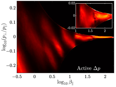
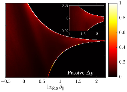
Figure 1: ‘Brazil plots’ – histograms of (local) $\beta$ versus $p_{\perp}/p_{\|}$ – formed by combining the data from all runs that have both active-$\Delta p$ and passive-$\Delta p$ simulations with the same parameters, as indicated by the ‘Passive?’ column of table 1 (for passive-$\Delta p$ simualations, the $\mbox{\boldmath{$\nabla$}}\,\mbox{\boldmath{$\cdot$}}\,(\hat{\bm{b}}\hat{\bm{b}}\,\mbox{\boldmath{$:$}}\,\mbox{\boldmath{$\nabla$}}\bm{u})$ force in 2 was artificially removed). The left panel combines all such active-$\Delta p$ simulations; the right panel combines all such passive-$\Delta p$ simulations. The colour (probability) scale is normalised differently for each $\beta$ to better show the main features, but is done so identically for the left and right panels. The insets zoom in on the right-hand regions of each plot. The clear differences between the active- and passive-$\Delta p$ simulations highlight the effect of the pressure-anisotropy feedback on the turbulence: active-$\Delta p$ cases maintain themselves primarily within the microinstability boundaries with small $|\Delta p|$, while passive-$\Delta p$ simulations (which have identical parameters otherwise, and similar turbulence amplitudes) have most of their volume artificially constrained by the hard-wall limiters. The basic conclusion is that the plasma employs dynamical pressure-anisotropy feedback, in addition to particle scattering (as more commonly discussed; Kasper et al., 2002; Hellinger et al., 2006; Bale et al., 2009), in order to limit its deviations from local thermodynamic equilibrium and stay within the kinetically stable region of parameter space.

A simple, familiar visual illustration of the effects of magneto-immutability is shown in figure 1, where we combine most of the simulations run as part of this work into two ‘Brazil’ plots. These are 2-D probability distribution functions (PDFs) of $\beta$ and temperature (pressure) anisotropy, illustrating the approximate magnitude of the deviation from pressure isotropy as a function of $\beta$. As mentioned earlier, its eponymous shape has usually been attributed to the action of microinstabilities scattering particles once $|\Delta|\gtrsim\beta^{-1}$ (the mirror and firehose thresholds; Kasper et al., 2002; Hellinger et al., 2006; Bale et al., 2009). The purpose of figure 1 is to compare simulations of 1–5 (left panel) to equivalent simulations where the dynamical feedback of $\Delta p$ has been artificially eliminated by removing $\mbox{\boldmath{$\nabla$}}\,\mbox{\boldmath{$\cdot$}}\,(\hat{\bm{b}}\hat{\bm{b}}\Delta p)$ in 2 and assuming an isothermal ion-pressure response (‘passive-$\Delta p$’ simulations; see §​ 3.1.3). Both sets of simulations include the effect of microinstabilities via hard-wall limiters at the firehose and mirror boundaries, which prevent $\Delta p$ from straying beyond the relevant instability thresholds. We see a clear difference between the two cases, with $\Delta p$ distributions strongly dominated by regions at the microinstability boundaries (the artificial limiters) in the passive cases, but not when $\Delta p$ feeds back on the flow. This demonstrates that, in its efforts to remain close to local thermodynamic equilibrium, the plasma has two separate methods at its disposal. The first – particle scattering through microinstabilities – has been discussed by Kasper et al. (2002), Hellinger et al. (2006), Bale et al. (2009) and other subsequent works. The second – the dynamical feedback from the pressure anisotropy – should be of similar importance for maintaining near-isotropy in most plasmas (see §​ 5.1), but has been largely ignored thus far.

3 Methods

3.1 CGL Landau-fluid model

Our computational study is based on the ‘CGL-Landau-fluid’ (CGL-LF) model of Snyder et al. (1997). This allows us to probe the effects discussed above without the complications of a true kinetic model (see §​ 2.3). The model solves 1–5 supplemented by the Landau-fluid closure for heat fluxes (described in §​ 3.1.1) and simple ‘hard-wall’ limiters on $\Delta p$ to approximate the effect of kinetic microinstabilities (§​ 3.1.2).

We use the finite-volume Athena++ code (White et al., 2016; Stone et al., 2020), modified to solve 1–5 in the conservative form detailed in appendix A. Briefly, this uses the total energy $E=p_{\perp}+p_{\|}/2+B^{2}/8\pi+\rho|\bm{u}|^{2}/2$ and the ‘anisotropy’ $\mathcal{A}\doteq\rho\ln(p_{\perp}\rho^{2}/p_{\|}B^{3})$ as conserved variables, the latter following Santos-Lima et al. (2014). We found through extensive numerical tests that using $\mathcal{A}$ leads to a solver that is more numerically robust than if $p_{\perp}/B$ or $p_{\|}B^{2}/\rho^{2}$ is used as the second conserved variable, particularly when there exists significant variation in $B$. Given that $\mathcal{A}$, and the equations themselves, become ill defined for $B\rightarrow 0$, we implement a numerical floor on $B$, below which the equations revert to standard adiabatic MHD. We use the piecewise parabolic method with an HLL Riemann solver (Toro, 2009); although we developed and tested various other HLLD-inspired solvers (Miyoshi & Kusano, 2005; Mignone, 2007), these were found to be insufficiently robust for this study (see §​ A.3.1).

The Riemann solver solves only the conservative part of 1–5, viz., that with $q_{\perp}=q_{\|}=0$ and $\nu_{\rm c}=0$. We evaluate the heat fluxes in the form described below (see 21) using operator splitting with slope limiters to ensure numerical stability and monotonicity of the solutions (Sharma & Hammett, 2007; Dong & Stone, 2009). We use the RKL1 super-time-stepping algorithm of Meyer et al. (2014) to allow for much larger time steps by stepping over the CFL condition that results from the small-scale diffusive form of the computational heat fluxes (although heat-flux-related time-step constraints are still relatively severe at high $\beta$ and high resolution). Collisional terms are evaluated at the end of each global time step $\delta t$ from the exact solution of $\partial_{t}p_{\perp}=-\nu_{\rm c}\Delta p/3$, $\partial_{t}p_{\|}=2\nu_{\rm c}\Delta p/3$ from $t$ to $t+\delta t$ (see 41). This method is implicit and numerically stable for any time step, and so has the property that adiabatic MHD can be easily recovered from the CGL-LF system by setting $\nu_{\rm c}\gg\delta t^{-1}$ (which also causes the heat fluxes to become negligible). Similarly, if we choose $\nu_{\rm c}\gtrsim\beta^{1/2}\omega_{\rm A}$ (see §​ 2.1.3), the method becomes a convenient, stable, and computationally efficient way to include a Braginskii-viscous stress in the standard MHD system.

Turbulence is driven via a large-scale incompressible forcing term $\bm{F}$ added to the right-hand side of 2. This applies only in the directions perpendicular to the mean magnetic field in order to drive primarily Alfvénically polarised fluctuations, and consists of the eight largest-scale modes in the box evolved in time as an Ornstein–Uhlenbeck process with correlation time $t_{\rm corr}=\tau_{\rm A}$ (where $\tau_{\rm A}$ is the box-scale Alfvén time). At each time step, its amplitude is adjusted to enforce a constant energy-injection rate $\varepsilon=\langle\rho\bm{u}\,\mbox{\boldmath{$\cdot$}}\,\bm{F}\rangle$ (see, e.g., Lynn et al., 2012).

3.1.1 Heat fluxes

In the ‘Landau-fluid’ heat fluxes 7–8, the $k_{\|}$ and $\nabla_{\|}=\hat{\bm{b}}\,\mbox{\boldmath{$\cdot$}}\,\mbox{\boldmath{$\nabla$}}$ contain $\hat{\bm{b}}$, which varies in space along with $c_{\rm s\|}^{2}=p_{\|}/\rho$. This implies that that $2c_{\rm s\|}^{2}({\sqrt{2\pi}c_{\rm s\|}|k_{\parallel}|+\nu_{\rm c}})^{-1}$ and $8c_{\rm s\|}^{2}[\sqrt{8\pi}c_{\rm s\|}|k_{\parallel}|+(3\pi-8)\nu_{\rm c}]^{-1}$ should rightly be considered operators that are not diagonal in either Fourier space or in real space, making them complex and computationally expensive to evaluate (see Snyder et al. 1997). For this reason, we use a simplified form, motivated by Sharma et al. (2006), in which $|k_{\|}|$ in the denominators of 7 and 8 is replaced by a constant $k_{L}$, which we take to be $2\times 2\pi/L_{\|}$ to approximate $k_{\|}$ of larger-scale motions. However, this substitution also leads to the undesirable property that, due to large parallel gradients at small scales, the heat flux, which is now diffusive, can become ${\gg}\rho c_{\rm s\|}^{3}$, the maximum possible heat flux (Hollweg, 1974a; Cowie & McKee, 1977). To mitigate this, we additionally limit $q_{\perp}$ and $\,q_{\|}$ to their maximum possible value deduced from 7 and 8, viz.,

$$q_{\perp,{\rm max}}\doteq\sqrt{\frac{2}{\pi}}c_{\rm s\|}p_{\perp},\quad q_{\|,{\rm max}}\doteq\sqrt{\frac{8}{\pi}}c_{\rm s\|}p_{\|}$$ (20)

(the second term in 7 is ${\sim}\Delta\,\delta B_{\|}/B\ll 1$ times smaller than the first, so we ignore its contribution). The heat fluxes are thus computed as

$$\widetilde{q}_{\perp}=q_{\perp{L}}\frac{q_{\perp,{\rm max}}}{q_{\perp,{\rm max}}+|q_{\perp{L}}|},\quad\widetilde{q}_{\|}=q_{\|{L}}\frac{q_{\|,{\rm max}}}{q_{\|,{\rm max}}+|q_{\|{L}}|},$$ (21)

where $q_{\perp{L}}$ and $q_{\|{L}}$ are evaluated using 7 and 8 with $|k_{\|}|=k_{L}$. We note that this approach effectively generalises the practice of limiting an MHD heat flux to be $|\bm{q}|\leq 5\phi\rho c_{\rm s}^{3}$ with $\phi\approx 0.3$ (Cowie & McKee, 1977), which is commonly used in MHD simulations (e.g., Vaidya et al., 2017).

The method (21) is somewhat ad hoc, which led us to explore various other approaches in some detail. One possibility for some regimes is to evaluate $|k_{\|}|$ along the constant mean field using Fourier transforms (Passot et al., 2014; Finelli et al., 2021), thus effectively approximating $|k_{\|}|=|\hat{\bm{b}}_{0}\,\mbox{\boldmath{$\cdot$}}\,\mbox{\boldmath{$\nabla$}}|$, rather than $|k_{\|}|=k_{L}$, in 7 and 8. However, with extensive testing, we found this approach to be more prone to numerical instability and more computationally expensive than the simpler method described above, when the fluctuations are large compared to the background magnetic field (as is explored here). In any case, because heat fluxes will be strongly modified by scattering from microinstabilities (see §​ 3.1.2 below), an exact evaluation of the Landau-fluid form (7)–(8) is likely irrelevant for detailed agreement to nonlinear collisionless physics, so long as the method captures their general influence on the flow (see §​ 2.1.3).

3.1.2 Microinstability limiters

As discussed in §​ 2.3, although aspects of the firehose and mirror instabilities are captured by 1–5 with the closure 7–21, their nonlinear saturation, which involves particle scattering and trapping, is not. We therefore artificially limit the pressure anisotropy to

$$-\Lambda_{\rm FH}\frac{B^{2}}{8\pi}<\Delta p<\Lambda_{\rm M}\frac{B^{2}}{8\pi},$$ (22)

where $\Lambda_{\rm FH}$ and $\Lambda_{\rm FH}$ define the firehose and mirror instability thresholds, respectively. By default, we set $\Lambda_{\rm FH}=2$ and $\Lambda_{\rm M}=1$, which describe the canonical versions of these instabilities, but our results do not depend strongly on this choice. Computationally, the limiters work by applying a large scattering rate ($\nu^{{\rm lim}}_{c}=10^{10}\tau_{\rm A}^{-1}$ in all simulations) to any region outside of 22, which quickly (within one time step) reduces $\Delta p$ to lie on the relevant instability boundary (see §​ A.1.1). We also apply this enhanced collisionality to the heat fluxes 7–8, thus strongly suppressing them in limited regions. This may be appropriate for mirror-limited regions, which show strong heat-flux suppression in simulations (Kunz et al., 2020), but it is likely much too strong in firehose-limited regions, which seem to be well described by the Braginskii estimate (Kunz et al., 2020), meaning it might be more appropriate to take $\nu_{\rm c}^{\rm lim}\sim\beta\hat{\bm{b}}\hat{\bm{b}}\,\mbox{\boldmath{$:$}}\,\mbox{\boldmath{$\nabla$}}\bm{u}$ (though this would be numerically complicated).

3.1.3 Passive-pressure-anisotropy simulations

For most simulations, in addition to the standard CGL Landau-fluid model (termed ‘active-$\Delta p$’ below), we have run an otherwise equivalent ‘passive-$\Delta p$’ simulation. The latter is identical to the former, except that the feedback of the pressure anisotropy into the momentum equation is artificially removed. Instead, we use an isothermal equation of state with the sound speed chosen to give the same value of $\beta$ as in the active-$\Delta p$ run. Note that these passive-$\Delta p$ runs still evolve the pressure anisotropy and include heat fluxes in an identical way to the standard CGL Landau-fluid model. In this way, the $p_{\|}$ and $p_{\perp}$ statistics can be compared directly to understand the feedback of the pressure-anisotropy stress on the flow.

In summary, a ‘passive-$\Delta p$’ simulation solves 1–5 using the same forcing, initial conditions, and parameters as a standard (‘active-$\Delta p$’) run, but, in 2 we remove the $\Delta p$ term and set $p_{\perp}=T_{i0}\rho$ with $8\pi\rho T_{i0}/B_{0}^{2}=\beta$ (a chosen initial parameter). This implies that the velocity and magnetic-field evolution in such a simulation is described by the isothermal MHD equations.

3.2 Study design

All simulations are run in a $L_{x}=L_{\|}=2L_{\perp}$ aspect ratio box of volume $V$, which has mean density $\rho=\rho_{0}$ and is threaded by a mean magnetic field $\bm{B}_{0}=B_{0}\hat{\bm{x}}$. The energy injection (forcing) level $\varepsilon$ is set to $\varepsilon=0.16v_{\rm A}^{3}/L_{\perp}$, which is chosen empirically to give $\mathcal{M}_{\rm A}\sim\delta u_{\perp}/v_{\rm A}\sim\delta B_{\perp}/B_{0}\sim 1/2$ in steady state for MHD, as needed for critical balance at the outer scale (from hereon, $v_{\rm A}$ will refer to the mean-field Alfvén speed $v_{\rm A}=B_{0}/\sqrt{4\pi\rho_{0}}$). We initialise with isotropic pressure $p_{0}$, chosen to yield the desired initial $\beta$, $\beta_{0}=8\pi p_{0}/B_{0}^{2}$. Recall that here and throughout, $\beta$ and $p_{0}$ refer to the ion contribution, and most simulations use $T_{e}=0$ by default in order to diagnose more easily the influence of pressure anisotropy. We do not use an explicit isotropic viscosity or resistivity in any simulations, relying on the grid to dissipate energy that reaches the smallest scales. Most simulations have a matching passive-$\Delta p$ run, which is set up as explained in §​ 3.1.3. With these default parameters, each simulation is specified by its initial ion $\beta$ and collisionality $\nu_{\rm c}$ (in units of $v_{\rm A}/L_{\perp}$; these are sometimes omitted for conciseness). These parameters then fix the expected interruption number from 19, assuming $\mathcal{M}_{\rm A}$ is not strongly modified by the effects of pressure anisotropy. The full set of simulations is listed in table 1.

We focus particularly on three simulations to probe both the collisionless and weakly collisional regimes with $\mathcal{I}\lesssim 1$ (meaning that pressure-anisotropy feedback is a significant effect). These use $\beta_{0}=10,\,\nu_{\rm c}=0$ (labelled CL10); $\beta_{0}=100,\,\nu_{\rm c}=33v_{\rm A}/L_{\perp}$ (B100); and $\beta_{0}=100,\,\nu_{\rm c}=0$ (CL100). CL10 and B100, which have a numerical resolution of $1120\times 560^{2}$, are chosen to have similar $\mathcal{I}\simeq 0.4$ but explore two different, collisionless and Braginskii, regimes laid out in §​ 2.1.3. CL100 (with resolution $560\times 280^{2}$) is chosen to examine a situation with stronger pressure-anisotropy feedback, $\mathcal{I}\approx 0.04$. The extremely small time steps required for the stable evaluation of the heat-flux terms make high-resolution simulations quite costly in wall-clock time, and so CL10 and B100 are initialised from the saturated state of lower-resolution simulations (see below). We then run them for only a relatively short time of $t\approx L_{\perp}/v_{\rm A}$, which is shorter than the outer-scale turnover time ${\simeq}2L_{\perp}/v_{\rm A}$, but longer than the time, $t\approx 0.1L_{\perp}/v_{\rm A}$, that it takes the new smaller scales to reach turbulent steady state (we observe the evolution of the energy spectrum to ensure that this is the case). This means that these simulations are useful for exploring detailed properties of the turbulence (e.g., turbulence structure and energy transfers), but the largest scales (those above around a quarter of the box scale) are not properly statistically averaged.

In addition to these simulations, we have a large array of other ones at low resolution ($400\times 200^{2}$). These are designed to explore how the physics of magneto-immutability varies with plasma parameters. ‘lrCL’ simulations are all collisionless, changing $\beta_{0}$ from ${\lesssim}1$ to ${\approx}100$ in order to probe the dependence of the turbulence on the interruption number from $\mathcal{I}\approx 0.04$ to $\mathcal{I}\gtrsim 1$. In simulations with $\beta_{0}\lesssim 1$, the plasma is heated, thus increasing $\beta$, rather rapidly, limiting the time they sit near their initial parameters. The ‘lrB’ simulations probe the collisionless, weakly collisional, and Braginskii-MHD regimes discussed in §​ 2.1.3 by keeping $\mathcal{I}\simeq 0.4$ approximately constant while changing $\beta_{0}$ and $\nu_{\rm c}$, with $\beta_{0}$ ranging from $30$ to $600$ and $\nu_{\rm c}\approx 0.33\beta_{0}\,L_{\perp}/v_{\rm A}$ (see 19). The ‘$\beta 16$’ simulations, which do not have a matching set of passive runs, all have $\beta_{0}=16$ and scan from the collisionless to the MHD regime in order to probe the approach to collisional MHD and compare more directly to the solar wind and/or kinetic simulations of A+22. Finally, we have carried out a number of simulations to test additional physical effects, including the effect of finite electron temperatures and different microinstability limiters.

Name	$\beta_{0}$	$\nu_{\rm c}\frac{L_{\perp}}{v_{\rm A}}$	$N_{\|}\times N_{\perp}^{2}$	$\mathcal{I}$	$\frac{\ell_{\perp}^{\rm WC}}{L_{\perp}}$	$\frac{\ell_{\perp}^{\rm CL}}{L_{\perp}}$	Passive?	Notes
CL10	10	0	$1120\times 560^{2}$	$\simeq 0.4$	N/A	$>1$	✓	Refined from lrCL10; run for $t\approx L_{\perp}/v_{\rm A}$
B100	100	33	$1120\times 560^{2}$	$\simeq 0.4$	$\simeq 1$	$\simeq 0.03$	✓	Refined from lrB100; run for $t\approx L_{\perp}/v_{\rm A}$
CL100	100	0	$560\times 280^{2}$	$\simeq 0.04$	N/A	$>1$	✓
lrB30	30	10	$400\times 200^{2}$	$\simeq 0.4$	$>1$	$\simeq 0.2$	✓
lrB100	100	33	$400\times 200^{2}$	$\simeq 0.4$	$\simeq 1$	$\simeq 0.03$	✓
lrB600	600	200	$400\times 200^{2}$	$\simeq 0.4$	$\simeq 0.2$	$\simeq 0.002$	✓
lrCL0.2	0.2	0	$400\times 200^{2}$	$\simeq 10$	N/A	$>1$	✓
lrCL1	1	0	$400\times 200^{2}$	$\simeq 4$	N/A	$>1$	✓
lrCL3	3	0	$400\times 200^{2}$	$\simeq 1$	N/A	$>1$	✓
lrCL10	10	0	$400\times 200^{2}$	$\simeq 0.4$	N/A	$>1$	✓
lrCL30	30	0	$400\times 200^{2}$	$\simeq 0.1$	N/A	$>1$	✓
lrCL100	100	0	$400\times 200^{2}$	$\simeq 0.04$	N/A	$>1$	✓
CL10fh1.4	10	0	$400\times 200^{2}$	$\simeq 0.4$	N/A	$>1$	✗	Reduced firehose limit $\Lambda_{\rm FH}=1.4$
CL10Te3	10	0	$400\times 200^{2}$	$\simeq 0.4$	N/A	$>1$	✗	Isothermal electrons, $\frac{T_{e}}{T_{i0}}=0.6$
CL10Te5	10	0	$400\times 200^{2}$	$\simeq 0.4$	N/A	$>1$	✗	Isothermal electrons, $\frac{T_{e}}{T_{i0}}=1.0$
$\beta$16$\nu$0	16	0	$400\times 200^{2}$	$\simeq 0.25$	N/A	$>1$	✗
$\beta$16$\nu$3	16	3	$400\times 200^{2}$	$\simeq 0.25$	$>1$	$\simeq 1$	✗
$\beta$16$\nu$6	16	6	$400\times 200^{2}$	$\simeq 0.5$	$>1$	$\simeq 0.4$	✗
$\beta$16$\nu$12	16	12	$400\times 200^{2}$	$\simeq 1$	$\simeq 1$	$\simeq 0.13$	✗
$\beta$16$\nu$24	16	24	$400\times 200^{2}$	$\simeq 2$	$\simeq 0.4$	$\simeq 0.05$	✗
$\beta$16$\nu$50	16	50	$400\times 200^{2}$	$\simeq 4$	$\simeq 0.13$	$\simeq 0.016$	✗
$\beta$16$\nu$100	16	100	$400\times 200^{2}$	$\simeq 8$	$\simeq 0.04$	$\simeq 0.006$	✗
$\beta$16$\nu$200	16	200	$400\times 200^{2}$	$\simeq 16$	$\simeq 0.016$	$\simeq 0.002$	✗
$\beta$16$\nu$400	16	400	$400\times 200^{2}$	$\simeq 32$	$\simeq 0.006$	$\simeq 0.0007$	✗

Table 1: A list of all simulations used in this article. Key input parameters are $\beta_{0}=8\pi p_{0}/B_{0}^{2}$ and $L_{\perp}\nu_{\rm c}/v_{\rm A}$, where the subscript ‘$0$’ refers to an initial value ($\beta$ decreases as $B$ grows and the turbulence causes ion heating). The interruption number $\mathcal{I}$ is computed from these initial parameters using 19. The collisionality regime is specified via $\ell_{\perp}^{\rm WC}$ and $\ell_{\perp}^{\rm CL}$, which are the approximate scales below which motions transition into the weakly collisional regime and collisionless regime, respectively. These are computed by equating $\nu_{\rm c}/\omega_{\rm A}(\ell_{\perp})=\beta^{1/2}$ and $\nu_{\rm c}/\omega_{\rm A}(\ell_{\perp})=1$, where $\omega_{\rm A}$ is estimated by $(2\pi v_{\rm A}/L_{\|})(\ell_{\perp}/L_{\perp})^{-2/3}$, as for a non-aligned critically balanced cascade (Goldreich & Sridhar, 1995; Schekochihin, 2022). A turbulent eddy of scale $\ell_{\perp}$ is in the Braginskii-MHD regime for $\ell_{\perp}\gtrsim\ell_{\perp}^{\rm WC}$, in the weakly collisional regime for $\ell_{\perp}^{\rm WC}\gtrsim\ell_{\perp}\gtrsim\ell_{\perp}^{\rm CL}$, and in the collisionless regime for $\ell_{\perp}\lesssim\ell_{\perp}^{\rm CL}$ (see §​ 2.1.3). The ‘Passive?’ column indicates whether an otherwise identical passive-$\Delta p$ simulation was run for comparison purposes. All simulations have $L_{\|}=2L_{\perp}$ and the energy injection rate $\varepsilon=0.16v_{\rm A}^{3}/L_{\perp}$.

3.3 Diagnostics

3.3.1 Energy and rate-of-strain spectra

The spectrum of a field $\phi$ is defined as

$$\mathcal{E}_{\phi}(k)=\frac{1}{\delta k}\sum_{|\bm{k}|=k}|\hat{\phi}(\bm{k})|^{2},$$ (23)

where $\hat{\phi}(\bm{k})$ is the Fourier transform of $\phi$, $|\bm{k}|=k$ indicates a sum over all modes that fall in the relevant bin of $k=\sqrt{k_{x}^{2}+k_{y}^{2}+k_{z}^{2}}$ or $k_{\perp}=\sqrt{k_{y}^{2}+k_{z}^{2}}$, and $\delta k$ is the width of the bin. The spectra are computed using a fine, logarithmically spaced $k$ or $k_{\perp}$ grid, removing the large-scale bins that do not contain any modes. Wavenumbers and spectra and are plotted in units of $L_{\perp}^{-1}$ and $\phi^{2}L_{\perp}$ (for various $\phi$), respectively, which will be omitted for conciseness in most figures.

Useful measures of turbulence structure are the spectra of the parallel and perpendicular rates of strain. These are formed via

$$\nabla_{\|}u_{\|}\doteq\hat{b}_{i}\hat{b}_{j}\nabla_{i}u_{j},$$

$$(\nabla_{\|}\bm{u}_{\perp})_{l}\doteq\hat{b}_{i}(\delta_{lj}-\hat{b}_{j}\hat{b}_{l})\nabla_{i}u_{j},$$

$$(\mbox{\boldmath{$\nabla$}}_{\perp}u_{\|})_{l}\doteq(\delta_{li}-\hat{b}_{i}\hat{b}_{l})\hat{b}_{j}\nabla_{i}u_{j},$$

$$(\mbox{\boldmath{$\nabla$}}_{\perp}\bm{u}_{\perp})_{kl}\doteq(\delta_{ki}-\hat{b}_{i}\hat{b}_{k})(\delta_{lj}-\hat{b}_{j}\hat{b}_{l})\nabla_{i}u_{j},$$ (24)

with the spectrum of a vector or tensor (e.g., $\nabla_{\|}\bm{u}_{\perp}$) computed by summing the spectra of each component. This gives a $\mbox{\boldmath{$\nabla$}}_{\perp}\bm{u}_{\perp}$ spectrum that is nearly identical to the dissipation spectrum ($\mbox{\boldmath{$\nabla$}}\bm{u}$ spectrum). Note that $\nabla_{\|}{u}_{\|}$ with this definition is exactly what must be minimised to minimise the generation of pressure anisotropy.

We also consider pressure anisotropy gradients defined in a similar way:

$$\nabla_{\|}\Delta p\doteq\hat{\bm{b}}\,\mbox{\boldmath{$\cdot$}}\,\mbox{\boldmath{$\nabla$}}\Delta p,$$

$$\mbox{\boldmath{$\nabla$}}_{\perp}\Delta p\doteq(\mathsfbi{I}-\hat{\bm{b}}\hat{\bm{b}})\,\mbox{\boldmath{$\cdot$}}\,\mbox{\boldmath{$\nabla$}}\Delta p$$

These will prove useful to quantify the reduction in the pressure-anisotropy stress $\mbox{\boldmath{$\nabla$}}\,\mbox{\boldmath{$\cdot$}}\,(\hat{\bm{b}}\hat{\bm{b}}\Delta p)$ compared to $\Delta p$ itself.

3.3.2 Structure functions

To diagnose the 3-D structure of turbulent eddies, we use three-point second-order structure functions, conditioned on the angle between the point-separation vector and the local field and/or the local perturbation. For any field $\phi$, these are defined as

$$S_{2}[\phi](\bm{\ell})=\langle|\phi(\bm{x}+\bm{\ell})-2\phi(\bm{x})+\phi(\bm{x}-\bm{\ell})|^{2}\rangle,$$ (25)

with the average taken over all $\bm{x}$. The separation vector $\bm{\ell}$ is conditioned on its angle to $\bm{B}_{\ell}=[\bm{B}(\bm{x}+\bm{\ell})+\bm{B}(\bm{x})+\bm{B}(\bm{x}-\bm{\ell})]/3$ to obtain parallel and perpendicular structure functions ($\ell_{\|}=\hat{\bm{b}}_{\ell}\,\mbox{\boldmath{$\cdot$}}\,\bm{\ell}$ and $\bm{\ell}_{\perp}=\bm{\ell}-\ell_{\|}\hat{\bm{b}}_{\ell}$ with $\hat{\bm{b}}_{\ell}\doteq\bm{B}_{\ell}/|\bm{B}_{\ell}|)$ (Cho & Lazarian, 2009; St-Onge et al., 2020). We also condition $\bm{\ell}$ on its direction with respect to the local field and flow perturbations to study the alignment of the turbulent fluctuations (Boldyrev, 2006; Chen et al., 2012; Mallet et al., 2015).

Following the computation of $S_{2}$, a useful diagnostic of the turbulence structure is the scale-dependent anisotropy $\ell_{\|}^{\phi}(\ell_{\perp})$ for a given field $\phi$. This is computed by solving the equation $S_{2}[\phi](\ell_{\perp})=S_{2}[\phi](\ell_{\|})$ using numerical interpolation.

3.3.3 Energy transfer functions

Energy-transfer functions are defined as in Grete et al. (2017) and A+22. The transfer function $\mathcal{T}_{q\rightarrow k}^{\rm AB}$ measures the average transfer of energy from $k$-shell $q$ to shell $k$ due to the interaction labelled AB. Here, $k$ shells are defined by the Fourier-space filtering operation,

$$\phi_{k}(\bm{x})=\sum_{|\bm{k}|=k}\,\hat{\phi}(\bm{k}){\rm e}^{{\rm i}\bm{k}\,{\bm{\cdot}}\,\bm{x}},$$ (26)

where $\hat{\phi}(\bm{k})$ is the Fourier transform of some field $\phi(\bm{x})$, and $|\bm{k}|=k$ represents those wavenumbers inside the logarithmic shell centred around $k$ (i.e., $\ln k-\tfrac{1}{2}{\rm d}\ln k\leq|\bm{k}|<\ln k+\tfrac{1}{2}{\rm d}\ln k$). Such a definition clearly satisfies the property $\phi(\bm{x})=\sum_{k}\phi_{k}(\bm{x})$ and represents the part of $\phi$ centred around wavenumber $k$. The label AB relates to the influence of different terms in 1–5: e.g., kinetic energy can be transferred between shells through the Reynolds stress in the momentum equation $\rho\bm{u}\,\mbox{\boldmath{$\cdot$}}\,\mbox{\boldmath{$\nabla$}}\bm{u}$, with

$$\mathcal{T}_{q\rightarrow k}^{\rm UU}=-\int{\rm d}\bm{x}\,\langle\sqrt{\rho}\bm{u}\rangle_{k}\,\mbox{\boldmath{$\cdot$}}\,\left[\bm{u}\,\mbox{\boldmath{$\cdot$}}\,\mbox{\boldmath{$\nabla$}}\langle\sqrt{\rho}\bm{u}\rangle_{q}\right],$$ (27)

or magnetic energy can be transferred to kinetic energy through $\bm{B}\,\mbox{\boldmath{$\cdot$}}\,\mbox{\boldmath{$\nabla$}}\bm{B}$. Further details of the specific transfer terms are given in §​ 4.4.

The full 2D transfer functions can give useful information on the locality of the cascade, but can be difficult to interpret quantitatively. Two useful reductions are the net energy transfer

$${\rm T}^{\rm AB}(k)=\sum_{q}{\mathcal{T}}^{\rm AB}_{q\rightarrow k},$$ (28)

and the flux

$$\Pi^{\rm AB}(k)=\sum_{q\leq k}\sum_{p>k}{\mathcal{T}}^{\rm AB}_{q\rightarrow p}.$$ (29)

The net transfer ${\rm T}^{\rm AB}(k)$ is the contribution of a given term ${\rm AB}$ in 1–5 to the rate of change of the energy spectrum at a particular $k$ (for example ${\rm T}^{\rm UU}(k)$ is the net contribution to the kinetic-energy spectrum at $k$ from the term $\rho\bm{u}\,\mbox{\boldmath{$\cdot$}}\,\mbox{\boldmath{$\nabla$}}\bm{u}$). In the inertial range in steady state, all terms should be zero because $\partial_{t}\mathcal{E}(k)=0$, unless there is a continual transfer of energy into or out of the particular shell or between terms (for example, a damping). The flux $\Pi^{\rm AB}(k)$ quantifies the transfer of energy across a particular $k$, such that the sum over all contributions AB measures the cascade rate. The interpretation of individual terms is less obvious, but gives interesting information about the dominant energy-transfer processes in the cascade (e.g., whether energy proceeds to smaller scales via transfers between $\bm{u}$ and $\bm{B}$, or due to transfers from larger scale $\bm{u}$ to smaller scale $\bm{u}$ directly).

4 Results

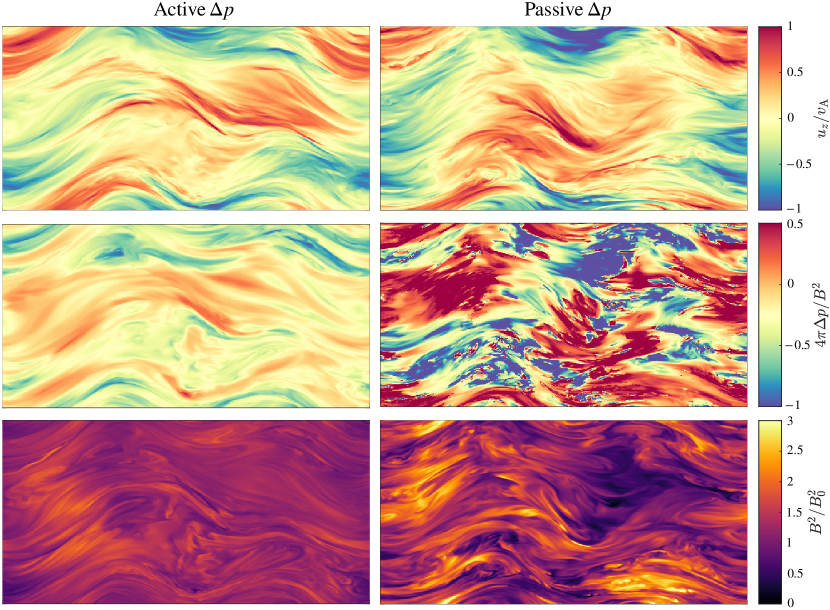
Figure 2: Visualization of $u_{z}/v_{\rm A}$ (top panels), $4\pi\Delta p/B^{2}$ (middle panels) and $B^{2}=|\bm{B}|^{2}$ (bottom panels) through an $x$-$y$ slice of the CL10 simulation with $\beta_{0}=10$ and $\nu_{\rm c}=0$ ($\mathcal{I}\approx 0.4$). Left panels show the active-$\Delta p$ run (which solves 1–5), and right panels show the passive-$\Delta p$ run, in which the $\mbox{\boldmath{$\nabla$}}\,\mbox{\boldmath{$\cdot$}}\,(\hat{\bm{b}}\hat{\bm{b}}\Delta p)$ force was artificially removed. While the fluctuations in $u_{z}$ look rather similar (i.e., the turbulence has a similar amplitude), magneto-immutability significantly reduces the variation in $B$ and $\Delta p$ in the active-$\Delta p$ run. Note that $-1<4\pi\Delta p/B^{2}<1/2$ is enforced by the limiters in both runs.

While the most astrophysically relevant consequences of magneto-immutability concern turbulent heating, it is necessary first to understand the details of how the field and flow self-organize to be magneto-immutable and how this characteristic manifests in the turbulence statistics. We thus start by diagnosing the basic effect of pressure anisotropy feedback by comparing probability distribution functions (PDFs) and Fourier spectra of various fluctuations in the active-$\Delta p$ simulations with those obtained in the passive-$\Delta p$ simulations (§§​ 4.1–4.2). We then consider the changes to the flow structure that are necessary in order to enable these effects in §​ 4.3, before diagnosing the viscous heating and cascade efficiency using energy transfer functions in §​ 4.4. Overall, the results show that, aside from a small range at the outer scale, magneto-immutability allows the system to set up a vigorous, nearly conservative cascade that is in most respects similar to standard MHD.

4.1 Reduction of the pressure anisotropy

A central result – that changes to the pressure anisotropy are suppressed by its feedback on the flow (magneto-immutability) – is illustrated in figures 1–4. Figure 1 shows the joint probability distribution function (PDF) of $\beta$ and $p_{\perp}/p_{\|}$ (the ‘Brazil plot’) for all simulations from the ‘lrCL’ and ‘lrB’ sets (18 in all; see table 1). We compare the set of CGL-LF simulations (left-hand panel) to the identical passive-$\Delta p$ simulations where the pressure-anisotropy feedback has been suppressed (right-hand panel). This diagnostic, although only qualitative (the total probability is normalised separately at each $\beta$ value for illustrative purposes, but done so identically for both simulation sets), clearly demonstrating the difference between the two. In particular, we see that the force on the flow from the pressure anisotropy causes most of the plasma to remain well within the microinstability limits. In contrast, the passive case, without $\Delta p$ feedback, has most of the volume stuck at the microinstability limits (the edges of the PDFs at high and low $p_{\perp}/p_{\|}$) because the turbulent fluctuations continuously push the plasma to positive and negative $\Delta p$. Similar results are demonstrated with a snapshot of the CL10 simulation in figure 2, where we again compare the active- and passive-$\Delta p$ simulations with otherwise identical parameters. While the perpendicular flows are of similar magnitudes, indicating similar turbulent fluctuation levels (top panels), the pressure-anisotropy variation (middle panels) is much smaller in the presence of pressure-anisotropy feedback. As a consequence, the variation in $B=|\bm{B}|$ is also suppressed: both $\Delta p$ and $B$ are driven by $\hat{\bm{b}}\hat{\bm{b}}\,\mbox{\boldmath{$:$}}\,\mbox{\boldmath{$\nabla$}}\bm{u}$, so suppressing one suppresses the other (more fundamentally, $\Delta p$ is driven by changes in $B$ and $\rho$).

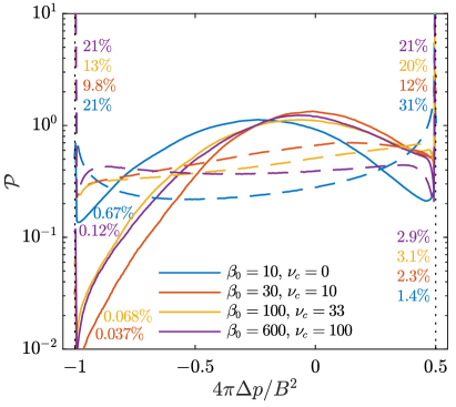
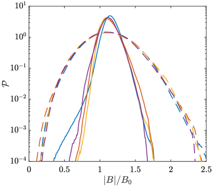
Figure 3: Left panel: PDFs of $4\pi\Delta p/B^{2}$ in the lrB simulation set, which explores the collisionless, weakly collisional, and Braginskii regimes at fixed $\mathcal{I}\approx 0.4$ (see §​ 3.2). Active-$\Delta p$ simulations are shown with solid lines and passive-$\Delta p$ simulations with dashed lines. The percentages shown on the left and right sides of the panel indicate the proportions (in volume) of each simulation that lie at the firehose and mirror thresholds, respectively (colours match the line styles; the larger numbers in the upper part of the plot are for the passive simulations). The effect of pressure anisotropy is relatively strong; only a few percent of the box lies at the mirror/firehose thresholds in the active-$\Delta p$ cases, while ${\sim}50\%$ of the box lies beyond these thresholds when $\Delta p$ has no effect on the flow. Right panel: PDFs of $B=|\bm{B}|$ for the same simulations. In active-$\Delta p$ cases, we see a factor-of-a-few decrease in the variance of $B$ (hence, ‘magneto-immutability’), which does not depend strongly on the regime of collisionality.

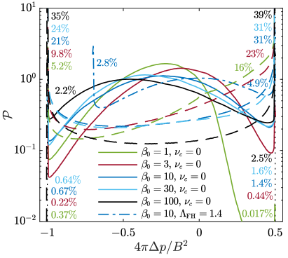
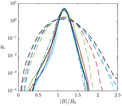
Figure 4: Same as in figure 3 but for the lrCL series of collisionless simulations with varying interruption number (see §​ 3.2). For very small interruption numbers (e.g., in the simulation with $\beta_{0}=100$, $\nu_{\rm c}=0$, $\mathcal{I}\simeq 0.04$), the proportion of the box at the mirror/firehose thresholds is larger (${\simeq}5\%$) because it is naturally driven to much larger values by the dynamics (cf. the passive simulation shown with the black dashed line). We also include a simulation with $\Lambda_{\rm FH}=1.4$ for comparison, to explore the possible effect of kinetic oblique-firehose modes limiting $\Delta p$ before the fluid firehose threshold (see §​ 3.1.2).

Figures 3 and 4 demonstrate the same ideas quantitatively, showing PDFs of $4\pi\Delta p/B^{2}$ and $B$ from the lrB simulation set in figure 3 (each with similar $\mathcal{I}\approx 0.4$) and from the collisionless lrCL simulation set in figure 4 (covering $\mathcal{I}\approx 0.04$, at $\beta_{0}=100$, to $\mathcal{I}>1$, at $\beta_{0}=1$). For each of the pressure-anisotropy PDFs (left-hand panels), we indicate the volume fraction of the box that sits at the mirror or firehose thresholds as a percentage (label colours match those of the curves, and the passive-$\Delta p$ cases are the larger numbers listed in the upper part of each panel). The PDFs have qualitatively different shapes between the active- and passive-$\Delta p$ simulations, with pressure-anisotropy feedback causing $\Delta p/B^{2}$ to peak near zero in the active-$\Delta p$ runs, as opposed to being nearly flat through the stable regions in the passive runs. As a consequence, the fraction of the plasma that sits at the microinstability thresholds is strongly reduced due to the pressure-anisotropy feedback on the flow. This fraction does increase modestly with decreasing interruption number (increasing $\beta_{0}$ in figure 4), but remains very small given that $\Delta p/B^{2}$ is effectively forced across a wider range with decreasing $\mathcal{I}$. We do not see any significant change with $\nu_{\rm c}$ across the lrB simulations (figure 3), all of which have $\mathcal{I}\approx 0.4$, showing that the collisionality regime (collisionless, weakly collisional, or Braginskii MHD) is of subsidiary importance. One exception to this is the mean negative $\Delta p$ in the collisionless cases, which becomes modestly more negative with increasing $\beta$ in collisionless simulations (figure 4), but is not seen in the weakly collisional or Braginskii regimes because the bulk $\nu_{\rm c}$ also depletes any mean $\Delta p$ that might otherwise develop. As discussed in A+22, this feature is likely related to turbulent heating occurring predominantly in the parallel direction via Landau damping (as approximated by the Landau-fluid closure). In figure 4, we also test the effect of a reduced firehose limit $\Lambda_{\rm FH}=1.4$, which is likely a better approximation for scattering from kinetic oblique firehose modes at very large scale separations $L_{\perp}/\rho_{i}$ (see §​ 3.1.2; Bott et al., 2021). This increases the proportion of the domain at the limiter thresholds (as expected, since the range between them is smaller) and decreases the mean $|\Delta p|$. The latter effect suggests that the asymmetry of the microinstability limits (i.e., the fact that $\Lambda_{\rm FH}>\Lambda_{\rm M}$) also contributes to the mean pressure anisotropy, but modest changes to $\Lambda_{\rm FH}$ do not seem to lead to any other qualitatively important changes, so we will not consider this further.

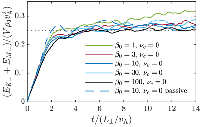
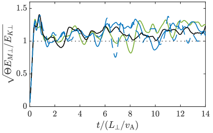
Figure 5: Time evolution of the total perpendicular energy (left panel) and the Alfvén ratio $r_{\rm A}=\sqrt{\Uptheta E_{M\perp}/E_{K\perp}}$ (right panel) for the lrCL set of collisionless simulations with varying interruption number. Note that $r_{\rm A}$ defined in this way (with $\Uptheta$ computed as a volume average) accounts for the effect of the mean pressure anisotropy on Alfvénic fluctuations (see 11). The dotted lines in each panel show the ‘expected’ values assuming $\delta u_{\perp}/v_{\rm A}=\delta B_{\perp}/B_{0}=1/2$: $E_{K\perp}+E_{M\perp}=V\rho_{0}v_{\rm A}^{2}/4$ and $r_{\rm A}=1$. We see that the bulk properties of collisionless turbulence are rather similar to standard MHD, even for $\mathcal{I}\ll 1$.

4.1.1 Turbulent energy

While the results shown in figures 1–4 clearly demonstrate the significant impact of the pressure-anisotropy feedback on the statistics of $B$ and $\Delta p$, it is important to confirm that this does not occur purely as a result of the viscous damping of those motions that would otherwise drive significant $\Delta p$. Because all simulations are driven with the same energy-injection rate $\varepsilon$, the simplest diagnostic of this is the turbulent fluctuation energy, which is shown in figure 5 for the lrCL runs (we plot $E_{K\perp}+E_{M\perp}\doteq\int{\rm d}\bm{x}\,(\rho|\bm{u}_{\perp}|^{2}+|\bm{B}_{\perp}|^{2}/4\pi)/2$, which includes only the fluctuating $y$ and $z$ components of $\bm{u}$ and $\bm{B}$). A fluctuation energy that decreased with decreasing $\mathcal{I}$ would imply a cascade efficiency that decreased with $\mathcal{I}$, as would be naïvely expected if fluctuations were increasingly strongly damped above the interruption limit (see §​ 2.2). Instead, we see in the left panel of figure 5 that such a decrease is quite small (compare, e.g., the active and passive cases at $\beta_{0}=10$), with a similar steady-state energy reached even at $\beta_{0}=100$ (the lowest $\mathcal{I}$ that we explore). Thus, we see that there is only modest viscous damping of pressure-anisotropy-generating fluctuations, a feature that we explore in greater depth below. Note that, in contrast, a single linearly polarised shear-Alfvén wave with similar amplitude would be strongly damped under these conditions because its fluctuations are confined to the plane set by the initial conditions and so it cannot rearrange itself to avoid generating large pressure anisotropies (Squire et al., 2016; S+19).

The right panel of figure 5 shows the Alfvén ratio, $r_{\rm A}=\sqrt{\Uptheta E_{M\perp}/E_{K\perp}}$, for some of the simulations. This should be approximately unity for Alfvénic turbulence. The time-dependent box-averaged mean anisotropy parameter $\Uptheta$ is included in $r_{\rm A}$ because an Alfvén wave satisfies $\delta B_{\perp}=\delta u_{\perp}\sqrt{4\pi\rho/\Uptheta}$ in the presence of a mean pressure anisotropy $\Delta p$ (see §​ 2.1.2; we set $\Uptheta=1$ for the passive simulation). Figure 5 shows that, after accounting for the change in the Alfvén ratio due to variation of the mean $\Delta p$ with $\mathcal{I}$ (see figure 4), the bulk properties of the turbulence are rather similar to MHD, with just a slight excess of magnetic energy (also observed in MHD; Müller & Grappin, 2005; Chen et al., 2013, see, e.g.,).

4.2 Alfvénic turbulence structure

We now diagnose the structure of the Alfvénic fluctuations in more detail, with the goal of understanding the similarities and differences between turbulence in high-$\beta$, weakly collisional plasmas and turbulence in standard MHD (Schekochihin, 2022). We will see that the basic statistics of the flow and magnetic field are surprisingly similar to MHD. More detailed diagnostics, which focus on compressive fields and components of the rate-of-strain tensor (see §​ 4.3), are needed to reveal the changes to the turbulent flow structure that enable the suppression of $\Delta p$ discussed in §​ 4.1.

4.2.1 Turbulent energy spectra at $\mathcal{I}\lesssim 1$

Figure 6: Kinetic (blue) and magnetic (red) energy spectra for simulations CL10, B100, and CL100, as labelled. Solid lines show CGL-LF (active-$\Delta p$) simulations, and dashed lines show isothermal MHD (passive-$\Delta p$) simulations. The dotted black lines indicate slopes of $k_{\perp}^{-3/2}$, $k_{\perp}^{-5/3}$, and $k_{\perp}^{-2}$ for comparison. We see spectra broadly consistent with a $k_{\perp}^{-3/2}$ scaling, although velocity spectra are steepened modestly by the effect of pressure anisotropy in the active-$\Delta p$ runs (however, they are clearly flatter than the ${\propto}k_{\perp}^{-2}$ spectrum observed in the hybrid-kinetic simulations of A+22). This demonstrates that vigorous turbulence, broadly resembling MHD, is maintained even when the feedback from the pressure anisotropy is strong ($\mathcal{I}<1$ in all cases). Note that the cutoff of the spectra at relatively larger scales seen in CL100 is simply a result of that run’s lower numerical resolution.

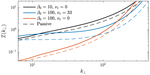
Figure 7: ‘Local’ interruption number defined by 31 (see also §​ 2.2.3). We show the three active-$\Delta p$ simulations whose spectra are given in §​ 4.2.1, comparing to the passive (MHD) runs with dashed lines. In the B100 simulation ($\beta_{0}=100$, $\nu_{\rm c}=33v_{\rm A}/L_{\perp}$), $\omega_{\rm A}$ depends on scale as per critical balance, $\omega_{\rm A}=k\sqrt{\delta u_{\perp}\delta B_{\perp}/\rho_{0}^{1/2}}$, which causes a slower increase in $\mathcal{I}$ with scale. Clearly, $\mathcal{I}(k_{\perp})\lesssim 1$ across a reasonable range in each simulation, indicating that much larger pressure anisotropies would be created without dynamical feedback from $\Delta p$ (as is the case for the passive simulations).

§​ 4.2.1 shows the kinetic (blue lines) and magnetic (red lines) spectra obtained in the CL10, B100, and CL100 simulations, again comparing active-$\Delta p$ simulations (solid lines) to the passive-$\Delta p$ simulations (dashed lines; note that this case is just isothermal MHD for velocity and magnetic fluctuations). The purpose of this comparison is to exhibit the extremely similar spectra in each case, demonstrating that vigorous turbulence survives even when the expected damping from pressure anisotropy is strong across a wide range of scales starting at the outer scale (as is the case for all three simulations shown here since $\mathcal{I}<1$). A careful examination reveals minor differences caused by the pressure-anisotropy feedback, in particular a slight steepening of the kinetic-energy spectrum compared to MHD. In all cases the magnetic spectra exhibit a scaling that is flatter than ${\sim}k_{\perp}^{-5/3}$ and closer to ${\sim}k_{\perp}^{-3/2}$ (shown with the dashed lines), although the exact slopes vary somewhat across the inertial range. We shall study the eddies’ 3-D structure and dynamic alignment in §​ 4.2.2.

Similar information in a different form is shown in figure 7. We integrate the spectra to obtain the scale-dependent amplitudes

$$\delta B_{\perp}(k_{\perp})^{2}=\frac{2}{V}\int_{k_{\perp}}^{\infty}{\rm d}k_{\perp}^{\prime}\,\mathcal{E}_{M\perp}(k_{\perp}^{\prime}),\quad\delta u_{\perp}(k_{\perp})^{2}=\frac{2}{V{\rho}_{0}}\int_{k_{\perp}}^{\infty}{\rm d}k_{\perp}^{\prime}\,\mathcal{E}_{K\perp}(k_{\perp}^{\prime}),$$ (30)

and then use these to compute the scale-dependent interruption number (see 19),

$$\mathcal{I}(k_{\perp})=\left(\beta\frac{\delta B_{\perp}}{B_{0}}\frac{\delta u_{\perp}}{v_{\rm A}}\right)^{-1}\max\left(1,\frac{\nu_{\rm c}}{\omega_{\rm A}}\right)$$ (31)

(we ignore the effect of the mean $\Uptheta$ on $v_{\rm A}$ and $\omega_{\rm A}$, as it does not make a significant difference for these qualitative estimates). Here $\omega_{\rm A}$ should be considered a function of scale as per critical balance, so we use $\omega_{\rm A}(k_{\perp})=k_{\perp}\sqrt{\delta u_{\perp}\delta B_{\perp}/{\rho}_{0}^{1/2}}$. We see that, while the estimated local interruption number is slightly larger for the CGL-LF simulations, because the turbulence amplitudes are modestly smaller, $\mathcal{I}(k_{\perp})$ nonetheless remains ${\lesssim}1$ throughout a wide portion of the turbulent cascade in each case. Since the damping rate of a linearly polarised Alfvénic perturbation is comparable to its frequency for for $\mathcal{I}\lesssim 1$ (i.e., for amplitude $\delta B_{\perp}/B_{0}\gtrsim\beta^{-1/2}\max[1,(\nu_{c}/\omega_{\rm A})^{1/2}]$), but the turbulent fluctuations exceed this amplitude throughout most scales of the simulations, the implication is that the fluctuations must be avoiding those motions that would cause strong damping in order for the cascade to proceed as observed. Also of note is the difference between the collisionless and weakly collisional regimes, as shown by the effectively flat $\mathcal{I}(k_{\perp})$ for the B100 simulation up to $k_{\perp}\approx 100$. This occurs because when $\omega_{\rm A}\ll\nu_{\rm c}$ (the weakly collisional and Braginskii MHD regimes; see §​ 2.1.3), the increasing frequency of the motions towards smaller scales cancels their decreasing amplitudes, conspiring to keep $\omega_{\rm A}\delta u_{\perp}\delta B_{\perp}$ approximately constant through the inertial range (see §​ 2.2.3). This breaks down once $\omega_{\rm A}\gtrsim\nu_{\rm c}$, which happens here for $k_{\perp}L_{\perp}\gtrsim 100$, around the expected scale based on the parameters (see table 1). Below this, $\mathcal{I}$ increases at smaller scales since the turbulent eddies are fast enough to be effectively collisionless.

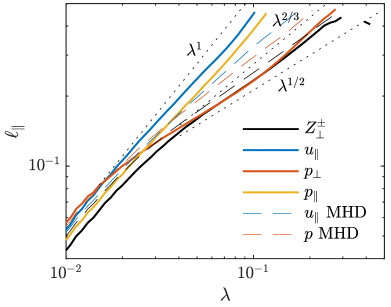
Figure 8: Structure functions in the $\beta_{0}=10$, $\nu_{\rm c}=0$ simulations. The left panel shows (3-point) second-order structure functions of $\bm{Z}_{\perp}^{\pm}$ (see §​ 3.3.2) with increments taken along the field (blue; $\ell_{\|}$), parallel to the local fluctuation in the opposite Elsässer variable $\bm{Z}_{\perp}^{\mp}$ ($\xi$; red), and perpendicular to the local fluctuation in $\bm{Z}_{\perp}^{\mp}$ ($\lambda$; black). Solid and dashed lines show the active-$\Delta p$ and passive-$\Delta p$ cases, respectively, with all length scales normalised to $L_{\perp}$. The scalings are very similar in both active and passive runs, and are broadly consistent with the expected $\lambda^{1/2}$, $\xi^{2/3}$, and $\ell_{\|}^{1}$ scalings of dynamic alignment (shown with dotted black lines). The right-hand panel shows the measured $\ell_{\|}(\ell_{\perp})$ for the same simulation, which is computed from the second-order structure functions of a variety of different quantities as labeled (this provides a measure of the average shape of an eddy for different variables). While $\bm{Z}_{\perp}^{\pm}$ and $p_{\perp}$ show the expected scale-dependent anisotropy $\ell_{\|}\sim\ell_{\perp}^{1/2}$ of a dynamically aligned cascade, $p_{\|}$ and $u_{\|}$ have nearly constant anisotropy $\ell_{\|}\sim 5\ell_{\perp}$ throughout the inertial range. This differs from MHD (dashed lines), where $u_{\|}$ and $p$ seem to follow $\ell_{\|}\sim\ell_{\perp}^{2/3}$, as expected for non-aligned eddies in a critically balanced cascade.

4.2.2 Three-dimensional anisotropy and alignment

Many previous works have studied the 3-D statistical structure of eddies in MHD turbulence, which has important implications for the cascade rate and intermittency (see Schekochihin, 2022, and references therein). Starting with Boldyrev (2006), these have argued that eddies become increasingly ‘dynamically aligned’ towards smaller scales, evolving into elongated sheet-like structures satisfying $\ell_{\|}\gg\xi\gg\lambda$ (where $\ell_{\|}$, $\xi$, and $\lambda$ are the eddy’s correlation lengths in the field-parallel direction, in the direction of the turbulent fluctuation, and in the mutually perpendicular direction, respectively). Motivated by its utility as a sensitive diagnostic of the Alfvénic fluctuations’ structure, in Figure 8 we illustrate the 3-D anisotropy of the CL10 simulations, computed using three-point structure functions (§​ 3.3.2). In the left panel, we show the directionally conditioned structure functions of $\bm{Z}^{\pm}_{\perp}=\bm{Z}^{\pm}-\hat{\bm{b}}(\hat{\bm{b}}\,\mbox{\boldmath{$\cdot$}}\,\bm{Z}^{\pm})$. Here $\bm{Z}^{\pm}=\bm{u}\pm\bm{v_{\rm A}}$ and $\bm{v}_{\rm A}$ is the local Alfvén speed $\bm{v}_{\rm A,eff}=\bm{B}\Uptheta^{1/2}(4\pi\rho)^{-1/2}$, with $\Uptheta$ and $\rho$ evaluated using their local three-point average ($\Uptheta=1$ for the passive simulation). The colours show different directions of the separation vector $\bm{\ell}=(\lambda,\xi,\ell_{\|})$, with $\ell_{\|}$ applying to separations within $15^{\circ}$ of the local $\hat{\bm{b}}$, $\xi$ to separations that are perpendicular ($>45^{\circ}$) to $\hat{\bm{b}}$ and are within $15^{\circ}$ of the direction of the local increment of $\bm{Z}^{\mp}_{\perp}$, and $\lambda$ to separations that are perpendicular to both $\hat{\bm{b}}$ and the $\bm{Z}^{\mp}_{\perp}$ increment (note that we use $\bm{Z}^{\mp}$ to define the directions of $\bm{Z}^{\pm}$ because nonlinear interactions are controlled by the opposite Elsässer variable). We see results that are quite similar to standard MHD turbulence (dashed lines), with $S_{2}$ flatter in the $\lambda$ direction than in the $\xi$ direction, and broadly consistent with (though modestly steeper than) the dynamically-aligned-MHD-turbulence scalings $S_{2}\sim\lambda^{1/2}$, $S_{2}\sim\xi^{2/3}$, $S_{2}\sim\ell_{\|}^{1}$ indicated by the dotted lines (Boldyrev, 2006; Mallet et al., 2015). The right panel compares the parallel-perpendicular anisotropy of eddies measured from different quantities in the turbulence. As seen in the left panel, the Alfvénic eddies are relatively similar to isothermal MHD, with $\ell_{\|}\sim\ell_{\perp}^{1/2}$ as expected for an aligned cascade. However, while in MHD the compressive quantities $u_{\|}$ and $p=T_{i}\rho$ seem to scale as $\ell_{\|}\sim\ell_{\perp}^{2/3}$, suggesting such fluctuations are unaligned and passively mixed by the critically balanced Alfvénic cascade (Lithwick & Goldreich, 2001; Schekochihin et al., 2009; Chen et al., 2012), the compressive fields in CGL-LF turbulence scale quite differently, with $p_{\|}$ and $u_{\|}$ having nearly constant anisotropy $\ell_{\|}\simeq 5\ell_{\perp}$ throughout the entire box. This provides the first hint of the differences caused by magneto-immutability, which will be discussed in more detail in the next section (§​ 4.3).

4.3 The rearrangement of flows and fields in magneto-immutable turbulence

Figure 9: Spectra of $\Delta p$ (purple lines), $p_{\perp}$ (green lines), $p_{\|}$ (yellow lines), and the magnetic pressure $B^{2}/8\pi$ (grey lines) for the same simulations as in §​ 4.2.1, and again with the passive-$\Delta p$ simulations shown with dashed lines. The dotted lines indicate the spectral scalings $\mathcal{E}\propto k_{\perp}^{-1}$ and $\mathcal{E}\propto k_{\perp}^{-5/3}$ (see §​ 4.3.3 for discussion). We see a significant difference between active- and passive-$\Delta p$ cases, with $\mathcal{E}_{\Delta p}\sim\mathcal{E}_{p_{\|}}\gg\mathcal{E}_{p_{\perp}}$ observed most clearly in the active-$\Delta p$ simulations (and, to a lesser degree, collisionless cases). The active-$\Delta p$ spectra bear encouraging resemblance to those seen in the hybrid-kinetic simulations of A+22.

§§​ 4.2.1–8 show that the CGL-LF system can sustain random, turbulent-like motions across a wide range of scales, even when those motions might be expected to be strongly damped by the effects of pressure anisotropy. The properties of the kinetic and magnetic fluctuations appear broadly similar to standard MHD, including relatively detailed measures such as the scale-dependent anisotropy and eddy-alignment intermittency. In this section, we focus on the differences compared to MHD, understanding how the turbulent cascade rearranges itself due to the pressure-anisotropy stress. We first present the numerical results, then speculate on theoretical explanations in §​ 4.3.3.

4.3.1 Pressure statistics

Let us first examine the spectra of pressure fluctuations, which are shown in §​ 4.3, again comparing active- and passive-$\Delta p$ for the CL10, B100, and CL100 simulations. Here, unlike for the kinetic- and magnetic-energy spectra, we see substantial differences due to the feedback of $\Delta p$ on the flow. The most obvious feature is the significant reduction and steepening of the pressure spectra in all active-$\Delta p$ runs. While the passive-$\Delta p$ simulations have quite flat spectra – approximately ${\propto}k_{\perp}^{-1}$ in B100 and yet flatter in the collisionless simulations – all three active cases exhibit pressure spectra ${\propto}k_{\perp}^{-5/3}$ across a reasonable range near the outer scales. Notably, the latter is in agreement with the hybrid-kinetic simulations of A+22, providing evidence that similar physics operates in their more realistic simulations. The steepening of pressure spectra due to the pressure-anisotropy feedback is clear evidence of the modified flow structure in the active-$\Delta p$ cases, despite their similar velocity spectra.

Another interesting feature of the active-$\Delta p$ pressure spectra is that $\mathcal{E}_{\Delta p}\sim\mathcal{E}_{p_{\|}}\gg\mathcal{E}_{p_{\perp}}$, while in the passive runs the difference between $\mathcal{E}_{p_{\|}}$ and $\mathcal{E}_{p_{\perp}}$ is far less pronounced (particularly for B100, where $\mathcal{E}_{p_{\|}}\sim\mathcal{E}_{p_{\perp}}$, as might be naïvely expected). This feature was also clearly observed in the hybrid-kinetic simulations of A+22. As discussed in more detail in §​ 4.3.3 and in A+22, it likely results from perpendicular pressure balance between $\mbox{\boldmath{$\nabla$}}p_{\perp}$ and the magnetic pressure $\mbox{\boldmath{$\nabla$}}B^{2}/8\pi$, while $p_{\|}$ is driven more strongly by $\hat{\bm{b}}\hat{\bm{b}}\,\mbox{\boldmath{$:$}}\,\mbox{\boldmath{$\nabla$}}\bm{u}$, thus dominating $\Delta p$. The basic feature seems generic to anisotropic collisionless (CGL) dynamics, occurring because $\delta p_{\perp}$ remains highly constrained by perpendicular pressure balance, while $\delta p_{\|}$ is not, affecting the plasma only through the parallel force (see §​ A.1.2 for a simple linear calculation to illustrate the effect). We provide evidence for the scenario in §​ 4.3 by plotting the spectra of the magnetic pressure $\mathcal{E}_{B^{2}/8\pi}$ (grey lines), which matches $\mathcal{E}_{p_{\perp}}$ very well below the forcing scales. In the CL10 simulation, where the feedback of the pressure anisotropy is only important at larger scales because $\mathcal{I}(k_{\perp})$ increases to ${\gg}1$ at small scales (see figure 7), the feature reverses to $\mathcal{E}_{p_{\|}}\simeq\mathcal{E}_{p_{\perp}}>\mathcal{E}_{\Delta p}$ for $k_{\perp}\gtrsim 200$ (there is no similar reversal for the passive-$\Delta p$ simulation). This is presumably the signature pressure-anisotropy feedback becoming subdominant (i.e., magneto-immutability no longer being important) once the driving of $\Delta p$ via $\hat{\bm{b}}\hat{\bm{b}}\,\mbox{\boldmath{$:$}}\,\mbox{\boldmath{$\nabla$}}\bm{u}$ becomes subdominant to standard MHD effects (the perpendicular pressure balance). We see hints that similar behaviour would occur in B100 and CL100, but at smaller scales than in CL10 (as expected), which unfortunately are unresolved in these simulations. Overall, the general similarity of the active-$\Delta p$ spectra, but not the passive-$\Delta p$ spectra, to the large-scale hybrid-kinetic results of A+22 is encouraging for the applicability of the CGL-LF model.

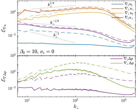
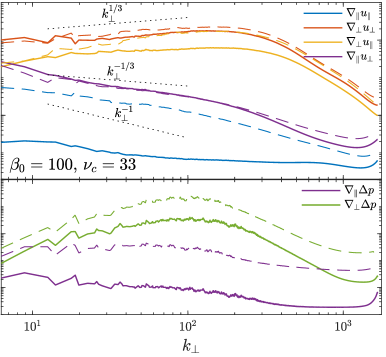
Figure 10: Rate-of-strain and pressure-gradient spectra in the CL10 and B100 simulations (left and right panels, respectively). Dashed lines show the equivalent passive-$\Delta p$ runs, while the colours indicate the specific strain direction considered. Details and definitions are described in §​ 3.3.1 (see 24 and 3.3.1); the dotted black lines indicate the ${\sim}k_{\perp}^{1/3}$, ${\sim}k_{\perp}^{-1/3}$, and $k_{\perp}^{-1}$ scalings (see text). While $\nabla_{\perp}u_{\perp}$, $\nabla_{\perp}u_{\|}$, and $\nabla_{\|}u_{\perp}$ are each relatively similar in active- and passive-$\Delta p$ runs, $\nabla_{\|}u_{\|}=\hat{\bm{b}}\hat{\bm{b}}\,\mbox{\boldmath{$:$}}\,\mbox{\boldmath{$\nabla$}}\bm{u}$, which is responsible for the creation of $\Delta p$, is markedly reduced when $\Delta p$ is active. Note that neither $\nabla_{\|}u_{\perp}$ nor $\nabla_{\perp}u_{\|}$ is similarly reduced, showing that the effect is not just a reduction in $u_{\|}$ or in $\nabla_{\|}$. The bottom panels show that $\nabla_{\|}\Delta p$ is suppressed more than $\nabla_{\perp}\Delta p$ in active-$\Delta p$ turbulence, which is a signal that the pressure-anisotropy stress is reduced beyond just the reduction in the variance of $\Delta p$, viz., $\mbox{\boldmath{$\nabla$}}\,\mbox{\boldmath{$\cdot$}}\,(\hat{\bm{b}}\hat{\bm{b}}\Delta p)/\Delta p_{\rm rms}$ is smaller in active-$\Delta p$ than in passive-$\Delta p$ turbulence.

4.3.2 Rate-of-strain spectra

Given that the pressure anisotropy is driven by the plasma motions, the pressure-anisotropy feedback must be driving important changes in the flow and magnetic-field structure, despite having only a small influence on the kinetic-energy spectrum (§​ 4.2.1). We diagnose this in figure 10 via the spectra of the local rates of strain, as defined in §​ 3.3.1. These reveal the expected substantial suppression of $\nabla_{\|}u_{\|}=\hat{\bm{b}}\hat{\bm{b}}\,\mbox{\boldmath{$:$}}\,\mbox{\boldmath{$\nabla$}}\bm{u}$ by the pressure anisotropy feedback, as needed to suppress the turbulently-driven fluctuations in $\Delta p$ and $B$. Of some interest is the comparison of $\nabla_{\|}u_{\|}$ to $\mbox{\boldmath{$\nabla$}}_{\perp}u_{\|}$ and $\nabla_{\|}\bm{u}_{\perp}$, with neither of the latter two significantly suppressed. This demonstrates that the system does not reduce $\hat{\bm{b}}\hat{\bm{b}}\,\mbox{\boldmath{$:$}}\,\mbox{\boldmath{$\nabla$}}\bm{u}$ purely via a reduction in field-parallel flows, or via the reduction of field-parallel gradients, but through the combination of the two. We see broadly similar features in the collisionless (CL10) and weakly collisional (B100) regimes, with the approximate spectral scalings $\mathcal{E}_{\nabla_{\perp}u_{\perp}}\propto k_{\perp}^{1/3}$, $\mathcal{E}_{\nabla_{\perp}u_{\|}}\propto k_{\perp}^{1/3}$, $\mathcal{E}_{\nabla_{\|}u_{\perp}}\propto k_{\perp}^{-1/3}$, and $\mathcal{E}_{\nabla_{\|}u_{\|}}\propto k_{\perp}^{-1/3}$ for both the active- and passive-$\Delta p$ simulations. As discussed below (§​ 4.3.3), the relatively flat $\mathcal{E}_{\nabla_{\|}u_{\|}}$ scaling may be a signature of some form of cascade of compressive fluctuations, since a $\hat{\bm{b}}\hat{\bm{b}}\,\mbox{\boldmath{$:$}}\,\mbox{\boldmath{$\nabla$}}\bm{u}$ spectrum that is dominated by linearly polarised Alfvénic fluctuations would be naïvely expected to scale as ${\sim}k_{\perp}^{-1}$. The most interesting difference between the collisionless and weakly collisional spectra is the closer-to-constant offset between the active and passive $\nabla_{\|}u_{\|}$ spectra in the weakly collisional case (i.e., the modestly steeper $\nabla_{\|}u_{\|}$ spectrum in B100), which may be a result of the pressure-anisotropy feedback being approximately constant across scales when $\omega_{\rm A}<\nu_{\rm c}$, rather than being dominated by the outer scale (see figure 7).

The lower panels in figure 10 show spectra of gradients of the pressure anisotropy. As is clear from the $\bm{u}$ evolution equation (2), it is not the pressure anisotropy itself that feeds back on the flow, but only its divergence

$$\mbox{\boldmath{$\nabla$}}\,\mbox{\boldmath{$\cdot$}}\,(\hat{\bm{b}}\hat{\bm{b}}\Delta p)=\hat{\bm{b}}\nabla_{\|}\Delta p-\hat{\bm{b}}\Delta p\nabla_{\|}\ln B+\Delta p\hat{\bm{b}}\,\mbox{\boldmath{$\cdot$}}\,\mbox{\boldmath{$\nabla$}}\hat{\bm{b}}.$$ (32)

Computing each of these terms separately, one finds that $\nabla_{\|}\Delta p$ is larger than the other terms, and there are no significant correlations between the different terms. Thus, if an active-$\Delta p$ run exhibits a lower ratio of $\nabla_{\|}\Delta p$ to $\mbox{\boldmath{$\nabla$}}_{\perp}\Delta p$ than an equivalent passive-$\Delta p$ run, this signifies that the effect of pressure anisotropy on the flow, $\mbox{\boldmath{$\nabla$}}\,\mbox{\boldmath{$\cdot$}}\,(\hat{\bm{b}}\hat{\bm{b}}\Delta p)$, is reduced beyond what would be assumed by just looking at the variance of $\Delta p$ or $\nabla_{\|}u_{\|}$. We see from figure 10 that this is indeed the case, viz., there is a secondary mechanism – the turbulence reduces $\mbox{\boldmath{$\nabla$}}\,\mbox{\boldmath{$\cdot$}}\,(\hat{\bm{b}}\hat{\bm{b}}\Delta p)$ beyond just $\Delta p$ (or $\mbox{\boldmath{$\nabla$}}\Delta p$) – which will further suppress the damping of plasma motions by pressure anisotropy.

We have examined a wide variety of correlations between the different terms that drive the pressure-anisotropy evolution (12). For example, one might imagine that a positive correlation between $\hat{\bm{b}}\hat{\bm{b}}\,\mbox{\boldmath{$:$}}\,\mbox{\boldmath{$\nabla$}}\bm{u}$ and $\mbox{\boldmath{$\nabla$}}\,\mbox{\boldmath{$\cdot$}}\,\bm{u}$ would aid in reducing $\Delta p$ generation, particularly at lower $\beta$ (see 13); or similarly for correlations between the heat fluxes and other terms in the $\Delta p$ evolution (12). However, directly comparing such measures between the active- and passive-$\Delta p$ simulations has not yielded any further effects that are worthy of note, so we do not discuss these here.

4.3.3 Possible theoretical interpretation

In this section we speculate on possible phenomenologies that could explain the observed pressure and rate-of-strain spectra in the inertial range below the forcing scales. We examine two qualitatively different possibilities: the first is that the pressures and $\hat{\bm{b}}\hat{\bm{b}}\,\mbox{\boldmath{$:$}}\,\mbox{\boldmath{$\nabla$}}\bm{u}$ are dominated by the residual magnetic-field variation that arises from a collection of linearly polarised Alfvénic fluctuations; the second is that they are dominated by a cascade of compressive fluctuations, which is set up around the forcing scales as the system rearranges itself. In the first scenario, the $\Delta p$ and $B^{2}$ spectra are the residual local ‘left-overs’ that cannot quite be eliminated by magneto-immutability; in the second, they are diagnosing another type of cascade or mixing of larger-scale fluctuations, similar to the passive slow-mode cascade in reduced MHD or gyrokinetics (Schekochihin et al., 2009; Kunz et al., 2015; Meyrand et al., 2019; however, unlike these gyrokinetic cases, the compressive and Alfvénic cascades could lack individually conserved invariants, meaning the distinction between them may be less precise than implied above). Motivated by the observation in §​ 4.3 that $\mathcal{E}_{p_{\|}}\gg\mathcal{E}_{p_{\perp}}$, we will imagine the compressive cascade to consist of oblique slow-magnetosonic-like modes, which, because they maintain perpendiclar pressure balance, satisfy $\delta p_{\perp}\ll\delta p_{\|}$. This property causes the mode’s frequency to scale as $k_{\|}v_{\rm th}$, rather than $k_{\|}v_{\rm A}$ (as for the MHD slow mode), as well as leading to significant damping by heat fluxes and/or collisions. Further details are given in §​ A.1.2 and Majeski et al. (2023).

Let us examine predictions for the rate-of-strain and pressure spectra for each possibility in turn, starting with the idea that finite-amplitude Alfvénic fluctuations dominate. In this case, a simple estimate for the spectrum of $\hat{\bm{b}}\hat{\bm{b}}\,\mbox{\boldmath{$:$}}\,\mbox{\boldmath{$\nabla$}}\bm{u}$ comes from 13, using $\hat{\bm{b}}\hat{\bm{b}}\,\mbox{\boldmath{$:$}}\,\mbox{\boldmath{$\nabla$}}\bm{u}\approx(1/2)B_{0}^{-2}{\rm d}(\delta B_{\perp}^{2})/{\rm d}t\sim\omega_{\rm A}\delta B_{\perp}^{2}/B_{0}^{2}$. For a critically balanced Goldreich–Sridhar cascade ($\delta B_{\perp}\propto k_{\perp}^{-1/3}$, $\omega_{\rm A}\propto k_{\perp}^{2/3}$), this suggests that $\hat{\bm{b}}\hat{\bm{b}}\,\mbox{\boldmath{$:$}}\,\mbox{\boldmath{$\nabla$}}\bm{u}\sim k_{\perp}^{0}$, or a $\hat{\bm{b}}\hat{\bm{b}}\,\mbox{\boldmath{$:$}}\,\mbox{\boldmath{$\nabla$}}\bm{u}$ spectrum $\mathcal{E}_{\nabla_{\|}u_{\|}}\propto k_{\perp}^{-1}$, which is clearly significantly steeper than observed (cf. the steepest dotted line in figure 10). However, this prediction is less rigorous than it seems because ignores the influence of magneto-immutability: larger $\delta B_{\perp}$, with larger local $\mathcal{I}(k_{\perp})$, will be more affected by $\Delta p$ forces, thus reducing $\hat{\bm{b}}\hat{\bm{b}}\,\mbox{\boldmath{$:$}}\,\mbox{\boldmath{$\nabla$}}\bm{u}$ below $\omega_{\rm A}\delta B_{\perp}^{2}/B_{0}^{2}$ and flattening its spectrum, perhaps to what is observed. However, the most straightforward estimate for this effect – that magneto-immutability would lead to $\Delta p$ fluctuations of approximately constant dynamical importance across scale (see §​ 2.2.3) – would suggest $\delta\Delta p\propto B_{0}^{2}$ or $\mathcal{E}_{\Delta p}\sim\mathcal{E}_{p_{\|}}\sim k_{\perp}^{-1}$, which also does not agree with what is observed (§​ 4.3). So, there is no obvious phenomenological explanation for the measured spectral slopes within this framework. As described above, the observation that $\delta p_{\perp}\ll\delta p_{\|}$ can be naturally explained by postulating that the finite-amplitude Alfvénic fluctuations are in perpendicular pressure balance with the magnetic-field-strength fluctuations, $\delta p_{\perp}\sim\delta(B^{2})$ (as observed in §​ 4.3). Because $\delta p_{\|}$ is instead driven by $\hat{\bm{b}}\hat{\bm{b}}\,\mbox{\boldmath{$:$}}\,\mbox{\boldmath{$\nabla$}}\bm{u}$ to $\delta p_{\|}\sim\beta\max(1,\omega_{\rm A}/\nu_{\rm c})\delta(B^{2})\gg\delta(B^{2})$, this suggests that $\delta\Delta p\sim\delta p_{\|}\gg\delta p_{\perp}$.

The other possibility – a compressive magnetosonic cascade – more naturally explains some spectral features, but appears to disagree with other key properties. Its most problematic aspect is that oblique CGL magnetosonic slow waves satisfy $\delta p_{\|}/\delta p_{\perp}\approx(5\beta+6)/2$ (see §​ A.1.2), a far larger ratio than what is observed in all three simulations shown in §​ 4.3. Furthermore, although the observed ratio $\delta p_{\|}/\delta p_{\perp}$ increases modestly with $\beta$, the increase is far slower than the predicted linear dependence, which, for example, would yield $\mathcal{E}_{p_{\|}}/\mathcal{E}_{p_{\perp}}\sim 1000$ in the CL100 simulation. This suggests that at least some other component or complication is necessary to decrease $\delta p_{\|}/\delta p_{\perp}$ well below the linear prediction to match the simulations. On the other hand, the observed spectral scalings of the rates of strain and pressure seem to be most naturally explained via a compressive cascade: if one postulates $u_{\|}\propto u_{\perp}\sim k_{\perp}^{-1/3}$ (assuming the compressive and Alfvénic cascades scale similarly), $\hat{\bm{b}}\hat{\bm{b}}\,\mbox{\boldmath{$:$}}\,\mbox{\boldmath{$\nabla$}}\bm{u}$ should scale as ${\sim}k_{\|}u_{\|}\propto k_{\perp}^{1/3}$, giving $\mathcal{E}_{\nabla_{\|}u_{\|}}\propto k_{\perp}^{-1/3}$, which is close to what is seen in figure 10. Predicted scalings of the other rates of strain ($\nabla_{\|}u_{\perp}\propto k_{\perp}^{1/3}$, $\nabla_{\perp}u_{\|}\propto k_{\perp}^{2/3}$, and $\nabla_{\perp}u_{\perp}\propto k_{\perp}^{2/3}$) are also consistent with what is observed, being the same as what is expected for passive slow-mode cascade in isothermal MHD (and indeed, the passive-$\Delta p$ rates of strain exhibit similar scalings in figure 10). In this scenario, pressure spectra would result predominantly from the passive mixing of larger-scale fluctuations, as opposed to local driving by $\hat{\bm{b}}\hat{\bm{b}}\,\mbox{\boldmath{$:$}}\,\mbox{\boldmath{$\nabla$}}\bm{u}$, which also naturally yields the observed scaling $\mathcal{E}_{p_{\|}}\propto\mathcal{E}_{p_{\perp}}\sim k_{\perp}^{-5/3}$ through the inertial range where $u_{\perp}\sim k_{\perp}^{-1/3}$, as well as explaining the similarity of the collisionless and weakly collisional simulations. Another interesting observation is the long parallel scale of $p_{\|}$ and $u_{\|}$ fluctuations (see $\ell_{\|}(\lambda)$ in figure 8b), which would be expected if for some reason the frequencies of Alfvénic and compressive fluctuations were matched around the outer scale.

Overall, we see a plausible agreement of the Alfvénic hypothesis with most diagnostics, although its predictions remain too qualitative to say much of substance. Its biggest flaw is the similarity of the collisionless and weakly collisional rate-of-strain and pressure spectra, which argues against pressure fluctuations being driven locally in scale by $\hat{\bm{b}}\hat{\bm{b}}\,\mbox{\boldmath{$:$}}\,\mbox{\boldmath{$\nabla$}}\bm{u}$. A compressive cascade alone cannot explain the observed spectra because the $\delta p_{\|}/\delta p_{\perp}$ ratio characteristic of linear slow-mode fluctuations is too large to fit the data (particularly the dependence on $\beta$); however, we cannot rule out their importance in some form (e.g., if $\delta p_{\perp}$ was dominated by residual Alfvénic fluctuations), and various other properties, particularly spectral scalings, seem to be more naturally explained via the compressive-cascade hypothesis. Clearly, more work is needed to make further progress.

4.4 Heating and energy fluxes

Perhaps the most interesting and macroscopically relevant impact of the pressure-anisotropy reduction through magneto-immutability is the suppression of viscous (pressure-anisotropy) heating that it entails. As discussed above, the effect implies that viscous damping is suppressed compared to naïve estimates for individual Alfvénic perturbations of similar amplitudes to the observed turbulent fluctuations, leading to a larger turbulent-cascade efficiency, with more energy transfered to small scales. Consequently, a larger fraction of the heating will occur through processes mediated by the small-scale turbulent cascade (e.g., Landau damping and nonlinear phase mixing around the ion gyroscale; Schekochihin et al., 2009; Kunz et al., 2018), as opposed to viscous damping of outer-scale eddies. These different heating mechanisms could in turn could have important thermodynamic consequences, modifying, for instance, the perpendicular-to-parallel ion heating fraction, or the ion-to-electron heating fraction.

In this section, we quantify these ideas by measuring directly the turbulent transfers and fluxes between scales. This allows us to measure the local damping due to pressure anisotropy across each scale in the cascade, and to determine the cascade efficiency by measuring the fraction of input energy that is lost into heat near the outer scale. This will again highlight a large difference between active- and passive-$\Delta p$ simulations, demonstrating that magneto-immutable turbulence is effectively conservative (no damping) below the outer scale.

4.4.1 Energy transfers and fluxes

As discussed in §​ 3.3.3, the turbulence energetics can be usefully quantified using ‘transfer functions’ $\mathcal{T}^{\rm AB}_{q\rightarrow k}$, which measure the energy transfer between shells in Fourier space due to different types of nonlinear interactions. Each of these transfers can involve several terms in the compressible system, so, as detailed in Grete et al. (2017), we combine relevant compressive terms into the non-compressive terms in order to reduce the number of quantities under consideration. The compressive terms are all individually very small and do not show interesting features, although they are necessary to include in order to respect energy conservation. Their full forms, as we compute them, are as defined in Grete et al. (2017), but we simply use the placeholder $\mathcal{C}_{\rm AB}$ to refer to them below. We follow Grete et al. (2017) in our nomenclature; ${\rm AB}={\rm UU}$ refers to the transfer between shells of the kinetic energy through $\bm{u}\,\mbox{\boldmath{$\cdot$}}\,\mbox{\boldmath{$\nabla$}}\bm{u}+\mathcal{C}_{\rm UU}$ (see 27), ${\rm AB}={\rm BU}$ refers to the transfer from magnetic to kinetic energy through $\bm{B}\,\mbox{\boldmath{$\cdot$}}\,\mbox{\boldmath{$\nabla$}}\bm{B}+\mathcal{C}_{\rm BU}$, ${\rm AB}={\rm UB}$ refers to the transfer from kinetic to magnetic energy through $\bm{B}\,\mbox{\boldmath{$\cdot$}}\,\mbox{\boldmath{$\nabla$}}\bm{u}+\mathcal{C}_{\rm UB}$, ${\rm AB}={\rm BB}$ refers to the transfer between shells of the magnetic energy through $\bm{B}\,\mbox{\boldmath{$\cdot$}}\,\mbox{\boldmath{$\nabla$}}\bm{B}+\mathcal{C}_{\rm BB}$, ${\rm AB}={\Delta p{\rm U}}$ refers to the transfer from the kinetic to thermal energy via the pressure anisotropy through $\mbox{\boldmath{$\nabla$}}\,\mbox{\boldmath{$\cdot$}}\,(\hat{\bm{b}}\hat{\bm{b}}\Delta p)$ (see below), and ${\rm AB}={\rm FU}$ refers to the transfer to kinetic energy from the external forcing. We compute transfers as a function of the isotropic $k$ as opposed to $k_{\perp}$, but results versus $k_{\perp}$ are similar.

As introduced in A+22, the only important new term compared to Grete et al. (2017) is that due to the pressure-anisotropy stress $\mathcal{T}_{q\rightarrow k}^{\Delta p{\rm U}}$. There is some freedom in the definition of this; A+22 use

$$\mathcal{T}_{q\rightarrow k}^{\Delta p\mathrm{U}}=\int\mathrm{d}\bm{x}\left\langle\sqrt{\rho}\bm{u}\right\rangle_{k}\,\mbox{\boldmath{$\cdot$}}\,{\rm sign}({\Delta p})\frac{\sqrt{|\Delta p|}}{B}\frac{\bm{B}}{\sqrt{4\pi\rho}}\,\mbox{\boldmath{$\cdot$}}\,\mbox{\boldmath{$\nabla$}}\langle\sqrt{|\Delta p|}\hat{\bm{b}}\rangle_{q},$$ (33)

which has the advantage that the square of $\langle\sqrt{|\Delta p|}\hat{\bm{b}}\rangle_{k}$ can be interpreted as the pressure anisotropy’s contribution to the thermal energy (Kunz et al., 2015), but the disadvantage of sign discontinuities that arise from $\sqrt{|\Delta p|}$. If we instead interpret the pressure-anisotropy stress as a damping of kinetic energy (as opposed to the transfer between energy reservoirs) a more natural definition is

$$\mathcal{T}_{q\rightarrow k}^{\Delta p\mathrm{U}}=\int\mathrm{d}\bm{x}\left\langle\sqrt{\rho}\bm{u}\right\rangle_{k}\,\mbox{\boldmath{$\cdot$}}\,\frac{\bm{B}}{\sqrt{4\pi\rho}}\,\mbox{\boldmath{$\cdot$}}\,\mbox{\boldmath{$\nabla$}}\left\langle\frac{\Delta p}{B^{2}}{\bm{B}}\right\rangle_{q}.$$ (34)

We have computed both versions, finding qualitatively similar results, but will focus on (34), because it fits more naturally with our focus on pressure-anisotropy damping. Note also that the influence of the sign-discontinuity issue of 33 was mitigated in A+22 because the $\Delta p$ distribution was mostly confined to negative values, but the spread of $\Delta p$ is somewhat broader in our simulations (see figures 3 and 4).

Figure 11: Important terms in the net energy-transfer spectra, as defined in §​ 3.3.3 and 28. The top panels show the simulations with $\beta_{0}=10$, $\nu_{\rm c}=0$ and the bottom panels show the simulations with $\beta_{0}=100$, $\nu_{\rm c}=33$, with the upper and lower subpanels for each showing the active- and passive-$\Delta p$ cases, respectively. Insets in the plots of the two active-$\Delta p$ cases show a zoom of the grey-box region. All transfers are normalised to $\varepsilon/(k/k_{f})$, which approximately represents the local cascade rate (see text). The different colours show different energy-transfer terms as labeled in the top panel: $\mathrm{T}^{\Delta p{\rm U}}$ is the transfer from $\bm{u}$ to thermal energy due to $\mbox{\boldmath{$\nabla$}}\,\mbox{\boldmath{$\cdot$}}\,(\hat{\bm{b}}\hat{\bm{b}}\Delta p)$; $\mathrm{T}^{\rm UU}$ is momentum transfer via $\bm{u}\,\mbox{\boldmath{$\cdot$}}\,\mbox{\boldmath{$\nabla$}}\bm{u}$; $\mathrm{T}^{\rm BU}$ is the contribution to kinetic energy from magnetic tension and pressure; $\mathrm{T}^{\rm BB}$ is the advection of $\bm{B}$ in the induction equation; $\mathrm{T}^{\rm UB}$ is the contribution to magnetic energy from field stretching; and $\mathrm{T}^{\rm FU}$ is the forcing contribution. In the active-$\Delta p$ simulations below the outer scale of the turbulence, we see little contribution of $\Delta p$ to the energy transfer, which shows directly that the effect of the pressure-anisotropy stress is minimised below the outer scale, even though the local interruption number is still smaller than unity in this range (see figure 7). In contrast, in the passive-$\Delta p$ simulations (bottom panel), the pressure anisotropy that develops is such that, if it did feed back on the flow, it would cause $\mathcal{O}(1)$ dissipation at all scales in the cascade (blue line), which would completely damp the turbulence.

Figure 12: The energy fluxes (see 29), which measure the transfer of energy across a particular $k$, for the two active-$\Delta p$ simulations with $\beta_{0}=10$, $\nu_{\rm c}=0$ (top panel) and $\beta_{0}=100$, $\nu_{\rm c}=33v_{\rm A}/L_{\perp}$ (bottom panel). We normalise to the forcing input $\varepsilon$, which implies that the total flux would be $\Pi/\varepsilon=1$ across the full inertial range for a conservative cascade with no damping. As also seen in §​ 4.4.1, although there is some energy loss due to $\Delta p$ at the outer (forcing) scale, at smaller scales the flux remains constant, showing that there is little energy damping through the inertial range.

In §​ 4.4.1, we plot the net energy transfers ${\rm T}^{\rm AB}(k)$ (see 28), which measure the net contribution from each term to the rate of change of the kinetic or magnetic energy spectrum at each $k$. For a conservative cascade, these are zero, because the transfer into a given shell from larger scales is balanced by the transfer out of the shell to smaller scales. Thus, ${\rm T}^{\rm AB}(k)$ provides a direct measure of the damping of kinetic or magnetic energy at each scale due to pressure anisotropy or other terms. To plot the results clearly, we normalise ${\rm T}^{\rm AB}(k)$ by the dimensional (Kolmogorov) estimate $\partial_{t}\mathcal{E}\sim ku_{k}\mathcal{E}\sim\varepsilon(k/k_{0})^{-1}$ (where $k_{0}=2\pi/L_{\perp}$); with this normalisation, a line that is constant and nonzero with $k$ symbolises a contribution that is of approximately constant importance compared a conservative cascade towards smaller scales. As above, we show the CL10 and B100 simulations, comparing to the results from the corresponding passive-$\Delta p$ simulations (lower subpanels). The thick black lines, which show the sum of all terms (excluding ${\rm T}^{\Delta p{\rm U}}$ for the passive runs), are approximately zero throughout the inertial range, as expected, with no clear difference between the active and passive runs. While the contribution from ${\rm T}^{\Delta p{\rm U}}$ is slightly negative in both CL10 and B100, indicating a slight damping of inertial-range motions, it is small compared to the cascade rate. Contrast this to the equivalent ${\rm T}^{\Delta p{\rm U}}$ from the passive simulations, which gives an indication of what the damping would be in the absence of feedback from $\Delta p$. Although this measurement is counterfactual – the cascade could not have proceeded in the presence of such strong damping – it concisely illustrates how motions driven by normal turbulence would be strongly damped, at a rate comparable to the cascade rate, across all scales. This is not entirely obvious for the collisionless case particularly, because the contribution to the kinetic energy from $\mbox{\boldmath{$\nabla$}}\,\mbox{\boldmath{$\cdot$}}\,(\hat{\bm{b}}\hat{\bm{b}}\Delta p)$ can be both positive and negative (it is negative definite in the Braginskii-MHD regime, but not otherwise; see 10). The effect of magneto-immutability all but eliminates such damping below the outer scale, leaving only a modest damping of outer-scale motions for the weakly collisional case.

§​ 4.4.1 shows similar information in a different form by plotting the contributions to the turbulent energy flux (29). We show only the active-$\Delta p$ runs because the comparison with passive simulations is less interesting in this case. Unlike the net transfers (§​ 4.4.1), individual terms in the fluxes are not easily interpreted because they do not include the diagonal $\mathcal{T}^{\rm AB}_{k\rightarrow k}$ transfer. While this diagonal contribution necessarily vanishes for the total energy flux, it dominates the transfer between different energy reservoirs, including the damping of the flow by the pressure anisotropy (blue line). Thus the fact that $\Pi^{\Delta p{\rm U}}$ is small and positive is not particularly relevant, while the individual lines are of interest only insofar as they indicate a contribution to the total flux (black lines). The most important feature that we observe is that the total energy fluxes are nearly constant for $10\lesssim k\lesssim 200$, consistent with the result of §​ 4.4.1 that there is little pressure-anisotropy damping through the inertial range (a slight decrease in $\Pi(k)$ is observed for B100, indicating a slight damping). The value of the $\Pi/\varepsilon$ in the inertial range is a direct measure of the cascade efficiency, which, as expected, is less than unity because there is some pressure-anisotropy damping near the forcing scales (the reduction of ${\simeq}25\%$ for C100 and ${\simeq}50\%$ for B100 is consistent with the total inferred pressure anisotropy heating, which is discussed below)

4.4.2 Pressure-anisotropy heating fraction and cascade efficiency

The net energy transfer ${\rm T}^{\Delta p{\rm U}}(k)$ also gives a convenient way to evaluate the total heating rate due to pressure anisotropy. Because the pressure-anisotropy (viscous) heating is confined to the outer scales (§​ 4.4.1), this is also a measure of the cascade efficiency – the energy that is available to cascade in the usual way to heat via small-scale collisionless mechanisms. Its precise value depends on the forcing scheme, since it mostly occurs at the outer scales where the forcing drives the flow, and could thus differ more significantly in systems with more realistic turbulence generation mechanisms (e.g., magneto-rotational turbulence; Kunz et al., 2016; Kempski et al., 2019). Nonetheless, its dependence on parameters ($\beta$ and the collisionality) is interesting to consider, as is a comparison to A+22.

We define

$$\mathcal{H}_{\Delta p}=\int_{k_{0}}^{k_{\rm max}}{\rm d}k\,{\rm T}^{\Delta p{\rm U}}(k),$$ (35)

so $\mathcal{H}_{\Delta p}/\varepsilon$ measures the fraction of the energy input that is converted into heat via pressure anisotropy up to wavenumber $k=k_{\rm max}$. Because the grid-scale dissipation in our simulations is non-physical – it is supposed to represent energy absorbed by the smaller scales, which would eventually cascade to mostly dissipate around the ion gyro-radius scale (Schekochihin et al., 2009) – it is most appropriate to choose $k_{\rm max}$ to lie near the bottom of the inertial range. We set $k_{\rm max}=100$ as appropriate for the resolution $400\times 200^{2}$, but the choice hardly affects the results for the active-$\Delta p$ simulations anyway, because almost all of the viscous heating is confined near the outer scales.

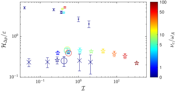
Figure 13: Net pressure-anisotropy heating rate $\mathcal{H}_{\Delta p}$ normalised to the cascade rate $\varepsilon$ from all simulations. The cascade efficiency, defined as the fraction of energy that participates in the cascade to small scales, is $1-\mathcal{H}_{\Delta p}/\varepsilon$. This is computed using the net transfer functions (§​ 4.4.1) by summing up the contributions from all $k\leq 100$, viz., $\mathcal{H}_{\Delta p}=\sum_{k\leq 100}\mathrm{T}^{{\rm U}\Delta p}(k)$, so as to exclude the grid scales. The marker style denotes the simulation set (see §​ 3.2 and table 1): circles denote the lrB set at constant $\mathcal{I}$, crosses denote the lrCL set with $\nu_{\rm c}=0$, and stars denote the $\beta 16$ set. We see that viscous (pressure-anisotropy) heating damps up to ${\simeq}45\%$ of the cascade in collisional regimes ($\nu_{\rm c}/\omega_{\rm A}\gtrsim 1$), and less in collisionless cases. This value is approximately constant for $\mathcal{I}\lesssim 10$ and independent of $\beta$ and $\nu_{\rm c}/\omega_{\rm A}$ (so long as $\nu_{\rm c}/\omega_{\rm A}\gtrsim 1$). The small symbols show the same computation from the passive-$\Delta p$ simulations; in this case the heating rate is larger than unity, because $\Delta p$ does not actually feed back on the flow. Such large values imply that if $\Delta p$ had not been reduced by magneto-immutability, it would have nearly completely damped the cascade.

We evaluate $\mathcal{H}_{\Delta p}$ for all of the lrCL, lrB, and $\beta 16$ simulations (see table 1), time averaging across the steady state of each. Results are shown in figure 13, plotted against the measured interruption number, with marker colour indicating the collisionality and marker style indicating the simulation set (lrCL, lrB, or $\beta 16$). The CGL-LF (active-$\Delta p$) simulations, shown with large symbols, have $\mathcal{H}_{\Delta p}$ between $\mathcal{H}_{\Delta p}\simeq 0.2\varepsilon$ for the collisionless simulations and $\mathcal{H}_{\Delta p}\simeq 0.45\varepsilon$ for the weakly collisional and Braginskii-MHD simulations at $\mathcal{I}\sim 1$, with no significant dependence on $\beta$. In other words, for this choice of forcing, the cascade efficiency is always above ${\simeq}50\%$, meaning most of the input energy can participate in an MHD-like turbulent cascade. Contrast this with the small symbols, which show the passive-$\Delta p$ simulations for lrCL and lrB, indicating what the pressure-anisotropy heating rate would be in the absence of magneto-immutability. The numerical values are of course meaningless in this case – the situation is counterfactual and having $\mathcal{H}_{\Delta p}>\varepsilon$ is clearly not possible – but, as above, it demonstrates that the motions involved in standard MHD Alfvénic turbulence would be strongly damped by pressure anisotropy were it not for the pressure-anisotropy feedback modifying their structure. From the $\beta 16$ simulations, we see also that $\mathcal{H}_{\Delta p}(\mathcal{I})$ remains relatively large up to large $\mathcal{I}$, despite the effective driving of pressure anisotropy fluctuations decreasing towards large $\mathcal{I}$ due to their larger $\nu_{\rm c}$. This shows that as $\mathcal{I}$ is decreased below ${\simeq}10$, the suppression of viscous heating is sufficiently strong that it balances the stronger driving of $\Delta p$ fluctuations that results from lower $\nu_{\rm c}$ (otherwise $\mathcal{H}_{\Delta p}$ would continue increasing below $\mathcal{I}\simeq 10$).

4.5 Effect of electron pressure

In all of the simulations presented so far, we have set $p_{e}=\rho T_{e}=0$, thus ignoring the influence of electrons. These add an additional isotropic pressure response that is worthy of exploration in case it interferes with magneto-immutability once it starts to dominate over the anisotropic ion pressure response. We explore this in figure 14 via the rate-of-strain spectra, motivated by the finding above that these showed a clear difference between CGL-LF and standard MHD (passive) simulations. We show the low-resolution versions of the spectra for the CL10 case already shown in figure 10, comparing them with two additional simulations that include electrons with $T_{e}/T_{i0}=1$ and $T_{e}/T_{i0}=5$ (here $T_{i0}$ is the initial ion temperature). We see no important differences, even for $T_{e}\gg T_{i}$, which further implies that the cascade efficiency is independent of $T_{e}/T_{i}$. This is expected since the plasma is already almost incompressible anyway, and an additional isotropic pressure should simply help it be even more so. The simulations of S+19 and Kempski et al. (2019) used a fully incompressible Braginskii-MHD model and found similar results.

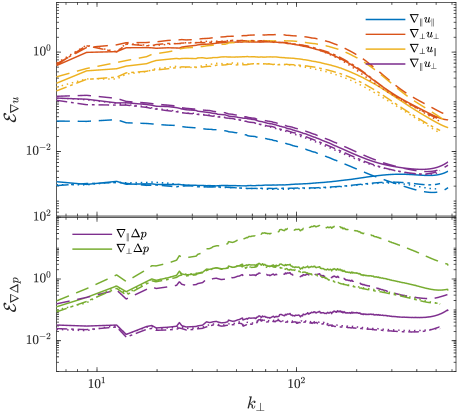
Figure 14: Rate-of-strain spectra at $\beta_{0}=10$, $\nu_{\rm c}=0$, comparing the effect of including an (isothermal) electron pressure with different $T_{e}$. We show $T_{e}=0$ (solid line), $T_{e}/T_{i0}=1$ (dot-dashed lines), $T_{e}/T_{i0}=5$ (dotted lines), and the passive-$\Delta p$ simulation (dashed lines). The plasma’s behaviour is almost identical to the $T_{e}=0$ case, because the isotropic electron pressure has little effect once motions are already nearly incompressible.

The isotropic fluid electron model is formally valid either when the plasma is semi-collisional (e.g., the ICM) or when electrons are cold. For the case of hot collisionless electrons, a separate electron pressure-anisotropy equation must be solved, which will add an electron contribution to the pressure anisotropy. Presumably this will generically act to enhance the influence of pressure anisotropy, even at large scales, while also bringing in a plethora of electron-scale kinetic instabilities driven by pressure-anisotropies, heat fluxes, and other non-Maxwellian features (e.g., Gary & Nishimura, 2003; Verscharen et al., 2022). However, because the Coulomb interspecies temperature equilibration is extremely slow and (as far as we are aware) there exist no plasma instabilities that act to decrease it (e.g., Zhdankin et al., 2021), there is not an obvious connection between the ion and electron thermodynamics. Thus, even though electron instabilities could strongly influence the electron temperatures (e.g., by limiting pressure anisotropies and heat fluxes; Verscharen et al. 2022), insofar as they remain very small-scale and unable to interact directly with ions, we do not expect them to have a strong influence on the large-scale ion dynamics other than through the pressure-anisotropy stress. That said, there is clearly more work needed to understand this complex physics better.

5 Discussion: uncertainties and observable effects

The numerical results presented herein have demonstrated how pressure anisotropy feeds back on Alfvénic turbulent flows at high $\beta$, minimising its own influence to reduce the variance of $B^{2}$ and the associated parallel viscous heating. The basic effect is neither surprising nor escapable, arising from the large pressure-anisotropy forces that are rapidly generated with any change of $B$ and act to oppose this change, in the same way that the large isotropic pressure forces that result from changes to density render fluids incompressible. However, our more detailed conclusions and quantitative features (e.g., the differences between collisional and collisionless results) do depend on the assumptions of the CGL-LF with hard-wall pressure-anisotropy limiters. In this section, we consider these in more detail by reference and comparison to the hybrid-kinetic simulations of A+22, particularly focusing on uncertainties relating to the interplay of magneto-immutability and microinstability scattering. We argue that most results are robust and compare well to A+22, which is promising more generally for the use of CGL-LF models in the study of weakly collisional plasmas. We also discuss various diagnostics that can be used in observations or kinetic simulations, where the comparison to passive-$\Delta p$ simulations – so useful in our analysis above – is not available.

5.1 Interplay between magneto-immutability and microinstabilities

Perhaps the largest uncertainty concerning the CGL-LF model relates to the influence of particle scattering through microinstabilities. As discussed in §​ 2.3, the ‘hard-wall-limiter’ method used here and in previous works is based on the idea that large-scale turbulent motions are extremely slow compared to microinstability-saturation time scales. This suggests that microinstabilities should instantaneously halt the growth of $|\Delta p|$ when it is driven beyond the stability thresholds, then instantaneously disappear again when the driving reverses and the plasma returns towards stability. In its practical implementation, the hard-wall-limiter model achieves this by taking $\nu_{\rm c}^{\rm lim}$ to be very large in unstable regions; however, kinetic theory and simulations show that the saturated scattering rate should actually be $\nu_{\rm c}\sim S\beta$, where $S\sim\hat{\bm{b}}\hat{\bm{b}}\,\mbox{\boldmath{$:$}}\,\mbox{\boldmath{$\nabla$}}\bm{u}$ is the shear driven by the turbulence. The effect on $\Delta p$ is similar – both hard-wall limiters and scattering with $\nu_{\rm c}\sim S\beta$ act to pin $\Delta p$ at the stability thresholds – but the differences could lead to inaccuracies. Furthermore, kinetic simulations have shown that the assumption that microinstabilities saturate and decay instantaneously compared to the turbulent motions is questionable. This is most acute for the mirror instability, which can limit $\Delta p$ growth via particle trapping through much of a macroscopic shearing time (Schekochihin et al., 2008; Kunz et al., 2014; Rincon et al., 2015). Decaying firehose and mirror fluctuations can also be extremely long lived, continuing to scatter particles even when not actively driven by the large-scale shear (Squire et al., 2017b; Kunz et al., 2020). Indeed, their decay rate, as it involves changing $B^{2}$, may itself be limited by the need to avoid creating unstable pressure anisotropies (Melville et al., 2016). Thus, it may not be appropriate to consider scattering only in unstable regions – rather, the continual driving will create a ‘soup’ of magnetic fluctuations that drive scattering across the entire plasma, putting it in the weakly collisional or Braginskii regime (Ley et al., 2023). This situation applies to almost any foreseeable kinetic numerical simulation, including those of A+22, but is at odds with the assumptions of our collisionless simulations, where we set $\nu_{\rm c}=0$ in stable regions.

We are thus left with some uncertainty between two limiting scenarios: in the first, scattering sites pervade the plasma; in the second, they exist only in spatiotemporal locations where the plasma is unstable. Reality, for astrophysically relevant scale separations, likely lies somewhere between these extremes. Comparing the microinstability-scattering estimate above, $\nu_{\rm c}\sim\beta S\sim\beta\omega_{\rm A}\mathcal{M}_{\rm A}^{2}$, with the Alfvénic interruption estimates discussed in §​ 2.2, we see that the $\nu_{\rm c}$ expected in the first scenario is exactly the collisionality required to maintain $\mathcal{I}\simeq 1$. Indeed, the correspondence is inherent in the estimate, since this $\nu_{\rm c}$ is simply that which is necessary to suppress the production of $\Delta p$ to a level where its influence becomes comparable to the magnetic forces. This shows that if the first scenario applies, all collisionless plasmas effectively become weakly collisional with $\nu_{\rm c}/\omega_{\rm A}\sim\mathcal{M}_{\rm A}^{2}$ and $\mathcal{I}\gtrsim 1$, meaning our $\mathcal{I}<1$ collisional and collisionless simulations are never formally applicable (see further discussion in A+22). More generally, in both scenarios, the scattering from microinstabilities and the pressure anisotropy stress (magneto-immutability) must be of similar importance to the plasma’s dynamics. Both effects limit $\Delta p$ to $|\Delta p|\lesssim B^{2}/4\pi$, and scale in the same way with $\beta$ and turbulence amplitude. As a corollary, there is no limit in which one or the other can be ignored, except in the presence of mean pressure anisotropy (resulting in microinstabilities but with no corresponding pressure-anisotropy stress; Bott et al., 2021).

In order to provide a more detailed theory, we must estimate the relative importance of two effects that scale in the same way with key parameters. This is difficult to do without kinetic simulations at asymptotically large scale separation, currently not feasible. The kinetic simulations of A+22 exhibited a box-averaged scattering rate consistent with $\nu_{\rm c}\simeq\beta S$ at $\beta=16$, or $\mathcal{I}\simeq 1$ (see their figure 12). While consistent with the first scenario (‘scattering everywhere’), given the modest separation (a factor ${\simeq}20$ between the outer scales and $\rho_{i}$), this does not constitute strong evidence against the second scenario in general, as there is no reasonable way to separate stable and unstable regions in the later stages of their simulations. This measured scattering rate, $\nu_{\rm c}\simeq\beta S$, also shows that either our $\beta 16\nu 6$ or $\beta 16\nu 12$ simulation should be directly comparable to the results of A+22 (see table 1). Indeed, for scales above $\rho_{i}$, most diagnostics appear relatively similar (e.g., pressure anisotropy spectra, the standard deviation of $B$ and $\Delta p$, and the viscous heating rate), with perhaps the most obviously significant large-scale difference being that the kinetic simulation drives itself to negative mean pressure anisotropy $\langle\Delta p\rangle$, while our $\beta 16$ simulations have $\langle\Delta p\rangle\approx 0$. A likely explanation for this lies in the crudeness of the scattering process from $\nu_{\rm c}$ in the CGL-LF model. In the kinetic simulation, negative pressure anisotropy builds over time as a result of the preferentially parallel heating due to Landau damping, seemingly reaching steady state once it triggers firehose scattering across the box (see their figures 3 and 5). However, once particle scattering from firehose fluctuations is triggered, rather than driving the plasma towards isotropy, it should be expected to maintain the plasma near the firehose threshold, allowing the system to maintain $\langle\Delta p\rangle<0$ even with a relatively high scattering rate. In contrast, the scattering included in our weakly collisional simulations with the CGL-LF model obviously drives the system towards $\langle\Delta p\rangle=0$, making it much harder for the system to maintain $\langle\Delta p\rangle<0$ in the weakly collisional case.

Given all of these uncertainties, our approach in this paper has been to explore a range of options within the confines of the fluid model. We have found that the pressure-anisotropy stress has a strong influence on the plasma’s dynamics across all collisionality regimes, for $\mathcal{I}\lesssim 10$ (see, e.g., figures 13 and 16). Thus even if the first scenario applies at astrophysically relevant scale separations, magneto-immutability should play an important role in the plasma’s dynamics, allowing a nearly conservative turbulent cascade to be set up below the forcing scales. Promisingly, A+22 measured a cascade efficiency of $55$–$60\%$ (meaning that $55$–$60\%$ of the input energy is processed via the turbulent cascade to kinetic scales), which compares very well to all of our weakly collisional and Braginskii-MHD simulations with $\mathcal{I}\lesssim 10$ (all of which have similar $\mathcal{H}_{\Delta p}$; see figure 13). Given the significant differences in physics and forcing, the correspondence could hint at ${\simeq}50\%$ being a quasi-universal (or at least minimum) cascade efficiency for weakly collisional plasmas, although an exploration of more realistic forcing mechanisms would be needed to confirm this. Overall, the use of the semi-phenomenological fluid model has been both a blessing and a curse: while we clearly miss very important kinetic effects, leading to the uncertainties discussed above, the influence of different physics can be explored more thoroughly by selectively studying different options, spanning wider parameter ranges, and comparing with counterfactual scenarios.

5.2 Observable consequences and diagnostics

Much of the evidence for magneto-immutability that we presented in this paper has relied on the direct comparison to the equivalent passive-$\Delta p$ or MHD simulations, a diagnostic luxury that is clearly not available in observations or even in kinetic simulations. In this section, we use the $\beta 16$ simulation set, which scans between the collisionless and MHD-like regimes by changing $\nu_{\rm c}$, to suggest various methods for diagnosing magneto-immutability in simulations or spacecraft data. There are several difficulties in this endeavour. First, the general effect of magneto-immutability is to make the weakly collisional turbulent plasma look more similar to MHD than it otherwise would; the corollary is that those differences that do persist are rather subtle. Secondly, there are other effects in MHD that tend to reduce the variance of $B$, which are unrelated to pressure anisotropy but very important in the near-Sun (low-$\beta$) solar wind especially. Thirdly, in either the solar wind or kinetic simulations, we will often not know a priori the effective particle scattering rate (see, e.g., Hellinger et al., 2011; Coburn et al., 2022), making it hard to disentangle the relative contributions of scattering and magneto-immutability to the reduction in the variance of $|\Delta p|$ (see §​ 5.1 above).

5.2.1 Constant-$B$ states in the solar wind – imbalance and spherical polarisation

In-situ spacecraft measurements in the solar wind and magnetosphere provide us with an unparalleled laboratory for studying fundamental plasma physics, and especially collisionless plasma turbulence (Chen et al., 2016; Verscharen et al., 2019). Regions with $\beta\gtrsim 1$ are regularly observed in the bulk solar wind, with values as high as $\beta\sim 10^{2}$ in specific regions (e.g., Cohen et al., 2017; Chen et al., 2021), making it a promising arena for studying the physics of pressure anisotropy and magneto-immutability. However, when working in this laboratory, we must recognise and consider other possible physics at play. In this context, a key point to note is that constant-$B$ ‘spherically polarised’ fluctuations, which are observed ubiquitously near the Sun (e.g., Belcher & Davis, 1971; Kasper et al., 2019), are most likely not related to pressure anisotropy and magneto-immutability. Here we discuss these and other possible mechanisms for reducing the variance of $|\bm{B}|$, which should be taken into account when interpreting observational data.

The robustness of spherically polarised states is related to the fact that any perturbation that satisfies

$$\frac{\delta\bm{B}}{\sqrt{4\pi\rho}}=\pm\bm{u},\quad B={\rm const},\quad p_{\perp},p_{\|},\rho={\rm const}$$ (36)

is an exact nonlinear solution of the Kinetic MHD system (1)–(5) (or even the standard MHD equations). Any such solution propagates at velocity $\mp\bm{B}_{0}\sqrt{\Uptheta/4\pi\rho}$, where $\bm{B}_{0}$ is the mean of $\bm{B}$ and $\delta\bm{B}$ is the remainder (Barnes & Hollweg, 1974). Since the solution (36) holds even if $|\delta\bm{B}|\gg|\bm{B}_{0}|$, these states are the natural nonlinear generalisation of linear Alfvén waves to large amplitudes. Their ubiquitous presence in the near-Sun solar wind is not unexpected given that Alfvénic perturbations grow in amplitude as they propagate outwards from the low corona due to the decreasing Alfvén speed (e.g., Völk & Aplers, 1973; Hollweg, 1974b). Given that they are observed consistently when $\beta\ll 1$, which necessarily implies $\mathcal{I}\gg 1$ for trans-Alfvénic motions, it seems unlikely that pressure anisotropy is playing an important role in their formation and sustenance (but see Tenerani & Velli 2020). Indeed, most aspects of their evolution can be well described by isothermal MHD (Hollweg, 1974b; Vasquez & Hollweg, 1998; Squire et al., 2020; Mallet et al., 2021).

Clearly, as exact nonlinear solutions, such states are not meaningfully turbulent, although there do exist turbulent-like states with very small $B$ variance that are similar to (36) (Dunn et al., 2023). But in order for such states to occur, the turbulence must be strongly imbalanced, with $|\bm{z}_{+}|=|\bm{u}+\bm{B}/\sqrt{4\pi\rho}|\gg|\bm{z}_{-}|=|\bm{u}-\bm{B}/\sqrt{4\pi\rho}|$ (or vice versa). This is the norm in the fast solar wind, but is less prevalent in the slow wind – presumably turbulence is also generically less imbalanced in other astrophysical plasmas with less ordered global structure. In this paper, we have not considered imbalanced turbulence, taking $|\bm{z}_{+}|\sim|\bm{z}_{-}|$ in all simulations, a limitation of our study that should be relaxed in future work. At any rate, the basic message is that there exist both MHD-related and pressure-anisotropy-related effects that reduce $B$ fluctuations in turbulence. In order to diagnose the influence of pressure anisotropy by considering the variance of $B$ between different regions, the imbalance must be taken into account, lest one inadvertently study the prevalence of nearly spherically polarised solutions instead. Similarly, in highly imbalanced high-$\beta$ turbulence, both pressure anisotropy and other reasons (e.g., wave growth in a plasma with a decreasing Alfvén speed) could cause the plasma to develop constant-$B$ spherically polarised fluctuations. Once formed, such fluctuations would not generate significant turbulent pressure anisotropy, in which case magneto-immutability might not play such an important role even for $\mathcal{I}\lesssim 1$.

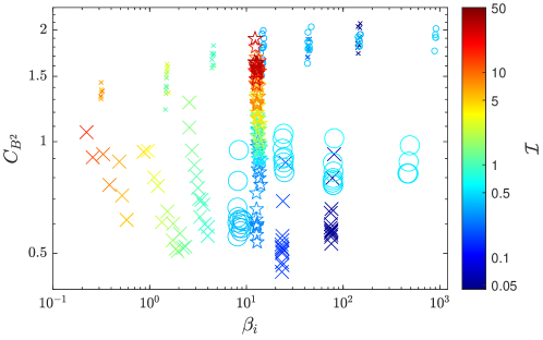
Figure 15: The variation in magnetic-field strength, or spherical polarisation, for all simulations, quantified in terms of $C_{B^{2}}$ given by 37. This measures the relative tendency for the components of $\bm{B}$ to be correlated in order to reduce the variation in $|\bm{B}|$. We plot multiple snapshots for each simulation, with the marker colour showing $\mathcal{I}$, which changes modestly during simulations due to heating and random fluctuations. Marker styles denote the simulation set and the small markers show the equivalent passive-$\Delta p$ simulations, with the same styles as in figure 13. We see a clear correlation between the magneto-immutability and the interruption number, even within individual simulations, and without any clear dependence on the collisionality regime. Further, even for $\beta\sim 1$, $C_{B^{2}}$ is reduced significantly by pressure-anisotropy effects. However, even the lowest values of $C_{B^{2}}$ observed here are larger than those regularly observed in the near-Sun solar wind due to the predominance of highly imbalanced, spherically polarised states 36.

To demonstrate more directly the reduction in the variance of $B$ across our simulations, in figure 15 we plot

$$C_{B^{2}}=\frac{(\delta B^{2})_{\rm rms}}{(\delta\bm{B}_{\rm rms})^{2}}=\frac{\langle(|\bm{B}|^{2}-\langle|\bm{B}|^{2}\rangle)^{2}\rangle^{1/2}}{\langle|\bm{B}-\langle\bm{B}\rangle|^{2}\rangle},$$ (37)

which was introduced by Squire et al. (2020) as a simple measure of the relative tendency of the components of $\bm{B}$ to become correlated in order to reduce the variance of $B$. This measure is mostly insensitive to the amplitude of the turbulence (small-amplitude, linearly polarised Alfvén waves have $C_{B^{2}}\approx 1/2$). For reference, Parker Solar Probe (PSP) observations and highly imbalanced expanding-box MHD simulations have $C_{B^{2}}$ in the range of $0.1$ to $0.3$ (Squire et al., 2020; Johnston et al., 2022). We plot $C_{B^{2}}$ from a number of snapshots of the $\beta 16$, lrCL, and lrB simulation sets, with each point coloured by the interruption number $\mathcal{I}$ (this can vary modestly between snapshots in a given simulation). As in figure 13, the MHD (passive-$\Delta p$) simulations are plotted with small markers, showing the expected higher variance of $B$ for otherwise similar conditions (see figures 3 and 4). The dependence on $\mathcal{I}$ is obvious, with lower-$\mathcal{I}$ simulations generally showing lower $C_{B^{2}}$ at otherwise identical parameters. We also see a tendency for modestly lower $C_{B^{2}}$ at lower $\beta$, which is likely related to the larger influence of magnetic pressure forces compared to thermal pressure forces at low $\beta$ (Vasquez & Hollweg, 1998). However, also of note is that all simulations, including those where pressure-anisotropy forces are very strong (low $\mathcal{I}$), show values of $C_{B^{2}}$ that are rather large compared to what is routinely observed in the solar wind or imbalanced turbulence (Kasper et al., 2019; Squire et al., 2020). It seems that magneto-immutability, while an important influence on the evolution of $B$, can never drive balanced turbulence arbitrarily close to keeping $B$ truly constant across the domain – imbalanced spherically polarised solutions are much better at this task.

5.2.2 Spectral diagnostics

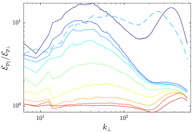
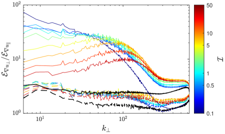
Figure 16: The left panel shows the ratio of pressure spectra $\mathcal{E}_{p_{\|}}/\mathcal{E}_{p_{\perp}}$, a simple diagnostic of magneto-immutability that should be readily observable in the solar wind. We show the simulations from the $\beta 16$ simulation set (see §​ 3.2 and table 1), with the line colour showing $\mathcal{I}$, and the black lines showing the corresponding results for isothermal MHD. The dashed line shows the lrB600, $\beta_{0}=600$ Braginskii-MHD simulation, to demonstrate that the observed decrease in $\delta p_{\|}/\delta p_{\perp}$ is not due to the change from the weakly collisional to the Braginskii-MHD regime at high $\mathcal{I}$ and $\beta_{0}=16$. The right panel shows the ratio of the spectra of $u_{\|}$ and $u_{\perp}$ in the parallel and perpendicular direction; $\mathcal{E}_{\nabla_{\|}u_{\perp}}/\mathcal{E}_{\nabla_{\|}u_{\|}}$ is shown with solid lines, and $\mathcal{E}_{\nabla_{\perp}u_{\perp}}/\mathcal{E}_{\nabla_{\perp|}u_{\|}}$ is shown with dashed lines (see figure 10 and §​ 3.3.1). The increase in $\nabla_{\|}u_{\perp}/\nabla_{\|}u_{\|}$ with decreasing $\mathcal{I}$ shows the change in the structure of the flow that results from the turbulence becoming more magneto-immutable at smaller collisionality. The lack of the same change in $\nabla_{\perp}u_{\perp}/\nabla_{\perp|}u_{\|}$ allows the effect to be considered separately from $u_{\|}$ itself, which may depend on the forcing and other parameters.

In §​ 4, we saw that, while kinetic- and magnetic-energy spectra remained rather similar in magneto-immutable turbulence compared to MHD, the rate-of-strain spectra and pressure anisotropy spectra did not. The $\beta 16$ simulation set provides a useful scan from low-$\mathcal{I}$ (small $\nu_{\rm c}$) to large-$\mathcal{I}$ collisional MHD, while other parameters ($\mathcal{M}_{\rm A}$ and $\beta$) remain similar. In figure 16 we plot two interesting ratios of spectra that clearly show the change in the structure of the turbulence at low $\mathcal{I}$. In the left panel, we show the ratio of parallel- to perpendicular-pressure spectra, which should be readily observable with in-situ solar-wind measurements. As discussed in §​ 4.3, it becomes larger than unity in magneto-immutable turbulence because of perpendicular pressure balance. We see the clear trend with $\mathcal{I}$: the higher-collisionality simulations ($\nu_{\rm c}/\omega_{\rm A}\gtrsim 50$, $\mathcal{I}\gtrsim 8$) all collapse down to $\delta p_{\|}\sim\delta p_{\perp}$, because the pressure anisotropy ceases to have a strong dynamical influence. In addition, the dashed line shows the lrB600 simulation, which is in the Braginskii regime but with $\mathcal{I}\approx 0.4$. This verifies that the observed change is not related to a transition between collisionality regimes (collisionless, weakly collisional, or Braginskii MHD). A similar diagnostic could be constructed from the slopes of the pressure spectra: in low-$\mathcal{I}$ turbulence, $\mathcal{E}_{p_{\perp}}$ flattens with scale while $\mathcal{E}_{p_{\|}}$ steepens, with the two spectra converging at small scales (see §​ 4.3); in contrast, when unaffected by the pressure-anisotropy feedback, the $p_{\perp}$ and $p_{\|}$ spectra have similar shapes.

Since we saw that the reduction in $\nabla_{\|}u_{\|}$ was one of the more obvious consequences of the pressure anisotropy feedback, the right panel compares the ratios of parallel-flow gradients $\mathcal{E}_{\nabla_{\|}u_{\perp}}/\mathcal{E}_{\nabla_{\|}u_{\|}}$ (solid lines) to those of perpendicular-flow gradients $\mathcal{E}_{\nabla_{\perp}u_{\perp}}/\mathcal{E}_{\nabla_{\perp}u_{\|}}$ (dashed lines). While the latter ratio is almost constant as a function of $\mathcal{I}$ and looks very similar to MHD (black lines), the former varies by a factor of at least ${\sim}10$ as the plasma transitions to collisional MHD. We also see that even at the highest collisionality ($\nu_{\rm c}/\omega_{\rm A}=200$, $\mathcal{I}\approx 50$), there remain clear differences in the flow structure compared to MHD.

In summary, these diagnostics could provide a useful way to understand and measure the influence of pressure-anisotropy feedback in more realistic simulations or observations. While the exact values of these metrics will depend on details (e.g., the forcing, $\mathcal{M}_{\rm A}$, and the imbalance), we expect that the qualitative features should be robust, especially the fact that $\mathcal{E}_{\nabla_{\|}u_{\perp}}/\mathcal{E}_{\nabla_{\|}u_{\|}}\gg\mathcal{E}_{\nabla_{\perp}u_{\perp}}/\mathcal{E}_{\nabla_{\perp}u_{\|}}$ and $\delta p_{\|}\gg\delta p_{\perp}$. This may allow one, for example, to diagnose and understand a transition to $\mathcal{I}\gg 1$ turbulence at small scales (as seen, e.g., for CL10 in §​ 4.3).

6 Conclusions

In this paper, we have studied the influence of fluctuation-generated pressure anisotropy ($\Delta p$) on magnetised plasma turbulence. The simulations and theory are based on a CGL-Landau-fluid model, which is effectively drift kinetics (Kulsrud, 1983) with heat fluxes approximated by a fluid closure that captures linear parallel Landau damping (Snyder et al., 1997). This makes it a reasonable model for collisionless plasma dynamics on scales far above the proton gyroradius. Indeed, our results compare well to the recent hybrid-kinetic simulations of A+22, which capture a much more comprehensive array of kinetic processes at the price of having a limited inertial range. Our results focus on the $\beta>1$ regime, where small changes of the magnetic-field strength lead to large pressure-anisotropy stresses on the plasma. This regime is relevant to many hot and diffuse astrophysical plasmas, including the intracluster medium and regions of the solar wind.

We show numerically, and argue theoretically, that the primary effect of the pressure-anisotropy stress on the fluid is to reduce its own influence via a dynamical feedback. This makes high-$\beta$ weakly collisional turbulence behave more like standard collisional MHD than would be naïvely expected, aside from a few important differences. The effect is straightforwardly understood by analogy with the origin of incompressibility in fluids, which results from the large $-\mbox{\boldmath{$\nabla$}}p$ force that rapidly opposes any flow with $\mbox{\boldmath{$\nabla$}}\,\mbox{\boldmath{$\cdot$}}\,\bm{u}\neq 0$ attempting to change the fluid’s pressure. With pressure and density tied together, this feedback eliminates density fluctuations. Analogously, there is a large force from $\mbox{\boldmath{$\nabla$}}\,\mbox{\boldmath{$\cdot$}}\,(\hat{\bm{b}}\hat{\bm{b}}\Delta p)$ that rapidly opposes any flow with $\hat{\bm{b}}\hat{\bm{b}}\,\mbox{\boldmath{$:$}}\,\mbox{\boldmath{$\nabla$}}\bm{u}\neq 0$ attempting to change the pressure anisotropy; since $\Delta p$ and $B$ are tied together, the feedback minimises magnetic-field-strength fluctuations in the turbulence. In the same way that the Mach number of a hydrodynamic flow quantifies the importance of pressure compared to inertial forces, the ‘interruption number’ $\mathcal{I}$ (introduced in S+19) quantifies the importance of pressure-anisotropic forces compared to magnetic tension (see §​ 2.2.3). The most important consequence of this physics is to reduce viscous heating from pressure anisotropy, confining it to a small range of scales near the outer scale so that most of the cascade remains nearly conservative. This increase in ‘cascade efficiency’ will in turn increase the fraction of heating that occurs via kinetic processes near and below the ion gyroscale (Schekochihin et al., 2009), thus influencing the thermodynamics of the plasma.

Compared to the previous work on Braginskii-MHD Alfvénic turbulence (S+19; Kempski et al., 2019), the results here explore plasmas in more realistic regimes at more modest $\beta$ and lower collisionality. Our results highlight the resilience of the pressure-anisotropy feedback mechanism: despite the much more complex evolution of the pressure anisotropy in the regimes studied here, particularly the effect of heat fluxes that act quasi-diffusively to smooth out $\Delta p$, we find that the basic features of magneto-immutable turbulence are robust. Our detailed analysis is aided by direct comparisons to ‘passive-$\Delta p$’ simulations, which are identical in setup but artificially remove the feedback of the pressure anisotropy on the flow. This allows us to compare, for example, the pressure-anisotropy distribution and viscous heating to the counterfactual situation in which $\Delta p$ evolved in standard MHD turbulence. A familiar illustration of this comparison is given in figure 1, where we plot the classic ‘Brazil plot’ of the joint PDF of $\beta$ and pressure anisotropy (e.g., Kasper et al., 2002; Hellinger et al., 2006). In the CGL-LF simulations, the pressure anisotropy is naturally constrained close to zero by magneto-immutability; in the passive-$\Delta p$ simulations, most of the volume sits instead at the microinstability boundaries, enforced here by artificial limiters.

A primary result of this study is that magneto-immutable turbulence behaves surprisingly similarly to standard MHD, illustrating the fundamental robustness of the MHD turbulent cascade. Specifically, despite the system having to rearrange itself to avoid dissipating most of the injected energy, the simulations show that saturated fluctuation amplitudes are similar to MHD for identical forcing, and the magnetic- and kinetic-energy spectra have slopes close to the expected $k_{\perp}^{-3/2}$ or $k_{\perp}^{-5/3}$. This has the effect of making the influence of pressure anisotropy rather subtle: rather than it causing some dramatic, obvious modifications to the system, magneto-immutability interferes and causes such turbulence to resemble MHD rather closely. That said, there are important differences that enable this behaviour, particularly that the system significantly suppresses the spectrum of the parallel strain $\hat{\bm{b}}\hat{\bm{b}}\,\mbox{\boldmath{$:$}}\,\mbox{\boldmath{$\nabla$}}\bm{u}$ (see figure 10), which reduces the magnitude of the $\Delta p$ and $B$ fluctuations (e.g., figures 4 and 15) and steepens the pressure spectra, leaving a characteristic signature with $\delta\Delta p\sim\delta p_{\|}\gg\delta p_{\perp}$ (§​ 4.3). These changes are summarised in figure 16, which shows how turbulence transitions from being magneto-immutable (low $\mathcal{I}$, blue) to collisional MHD (high $\mathcal{I}$, red and black), demonstrating how such effects could be diagnosed and studied with in-situ solar-wind observations (see §​ 5.2).

Macroscopically, the most important effect of magneto-immutability is to suppress strongly the viscous heating that would otherwise almost completely damp the turbulent cascade. This leaves an effectively conservative cascade below the forcing scales that processes ${\approx}50\%$ to ${\approx}80\%$ of the input energy (depending on the regime; see §§​ 4.4.1 and 13). While the particular values for the cascade efficiency will depend on the forcing scheme, so will certainly differ for more realistic systems (e.g., those driven by large-scale instabilities), the general point is that the magneto-immutability modifies the conversion between mechanical and thermal energy in the plasma. This could have interesting consequences for its macroscopic thermodynamics. For example, important quantities like the fraction of turbulent energy that heats ions versus electrons, or in the perpendicular versus parallel directions, can depend on the cascade efficiency and viscous heating. A specific application where such physics could have direct consequence is the intracluster medium, in which turbulent heating is thought to offset a large fraction of radiative losses to mitigate cluster cooling flows (e.g., Churazov et al., 2004; Zhuravleva et al., 2014). Kunz et al. (2010) suggested that, by forcing the plasma to adjust its parallel rate of strain, pressure anisotropy could regulate turbulent heating to maintain naturally the plasma’s thermal stability against Bremsstrahlung cooling (with viscous heating ${\propto}B^{4}T^{-5/2}$ at fixed gas pressure increasing faster than cooling ${\propto}T^{-3/2}$ as the temperature drops). While the details of their scheme differ from the turbulent heating studied here (specifically, Kunz et al. 2010 assumed that kinetic microinstabilities provide the primary regulation mechanism by contributing to, and thereby regulating, the total parallel rate of strain), the basic idea – that suppression of the parallel rate of strain provides a strong constraint on the heating rate – is analogous to magneto-immutability. Thus, similar thermal-stability considerations may apply to magneto-immutable turbulence, with the modification that it is the large-scale (as opposed to the small-scale) adjustment to the parallel rate of strain that regulates the viscous heating. At the same time, the mechanism would allow some of the injected energy (the cascade efficiency) to pass into a turbulent cascade, as needed to explain observations of small-scale fluctuations on scales below the Coulomb mean-free path (Zhuravleva et al., 2019; Li et al., 2020). The effectiveness of such a mechanism likely depends on how fluctuations are driven (the forcing), as well as complications such as anomalous particle scattering (see §​ 5.1), so further study in more realistic settings is clearly needed.

Due to the ad-hoc nature of some approximations that were needed for the CGL-LF model, our study is beset with some serious (but, we think, ultimately not game-changing) uncertainties. The most important one is the influence of kinetic microinstabilities, e.g., the firehose and mirror instabilities, which grow extremely rapidly compared to large-scale motions in regions of large $|\Delta p|$. We use simplified hard-wall limiters (Sharma et al., 2006), but it is clear from kinetic simulations that these could miss important effects such as long-lived fluctuations that continue to scatter particles even in stable regions. In this context, our study complements the recent hybrid-kinetic simulations of A+22, which capture all such complexities (except the electron physics), but suffer from unavoidable limitations related to low scale separation. This complicates the exploration of the inertial-range $k_{\perp}\rho_{i}\ll 1$ turbulence in the system, both because the microinstabilities’ growth and saturation are not particularly fast compared to the integral-scale motions, and because $\rho_{i}$-scale physics (e.g., the damping of perturbations; Foote & Kulsrud, 1979) can start to interfere directly with scales comparable to the size of the box. Nonetheless, our comparable simulations that have an imposed collisionality to approximate the effects of microinstabilites (see §​ 5.1), provide a good match to most features observed in A+22. This includes most spectra of Alfvénic and compressive quantities, $\Delta p$ and $B$ distributions (aside from a mean $\langle\Delta p\rangle<0$ in A+22), and the cascade efficiency, which is ${\simeq}55\%$ in A+22 (matching effectively all of the weakly collisional and Braginskii-MHD simulations; see figure 13). Thus, a secondary result of our work is that the CGL-LF model provides an accurate and relatively simple way to model weakly collisional plasmas in high-$\beta$ regimes. That said, there remain significant caveats, and working to build a better bridge between the regimes accessible via the CGL-LF and hybrid-kinetic approaches should be a priority for future work.

Appendix A Numerical method and validation

In this appendix we discuss various features of the numerical implementation of our equations. We first give the relevant equations and other results that are needed for the conservative part of the equations (i.e., for the CGL equations; §​ A.1), followed by those needed for the heat fluxes and collisions (§​ A.1.1). We then present some simple wave tests and discuss a collection of numerical problems that arose for this system, speculating on their possible causes. As part of this discussion, we present a more accurate Riemann solver that works well for some problems, but has turned out to be too unreliable for large-amplitude (large-$\delta B_{\perp}$) turbulence simulations.

A.1 Conservative form

As is standard for finite-volume implementations, we solve 1–5 in the conservative form

$$\frac{\partial\bm{U}}{\partial t}+\frac{\partial\bm{F}_{x}}{\partial x}+\frac{\partial\bm{F}_{y}}{\partial y}+\frac{\partial\bm{F}_{z}}{\partial z}+\mbox{\boldmath{$\nabla$}}\,\mbox{\boldmath{$\cdot$}}\,\bm{Q}=0,$$ (38)

where

$$\bm{U}=\begin{pmatrix}\rho\\ m_{x}\\ m_{y}\\ m_{z}\\ E\\ \mathcal{A}\\ B_{x}\\ B_{y}\\ B_{z}\end{pmatrix}=\begin{pmatrix}\rho\\ \rho u_{x}\\ \rho u_{y}\\ \rho u_{z}\\ p_{\perp}+\frac{1}{2}p_{\|}+\frac{1}{2}B^{2}+\frac{1}{2}\rho|\bm{u}|^{2}+p_{e}\ln p_{e}\\ \rho\ln(p_{\perp}\rho^{2}/p_{\|}B^{3})\\ B_{x}\\ B_{y}\\ B_{z}\end{pmatrix};$$ (39)

$\bm{F}_{x}$, $\bm{F}_{y}$, and $\bm{F}_{z}$ are the CGL fluxes; and $\bm{Q}$ are the heat fluxes, which are defined below (for simplicity of notation, we normalise $\bm{B}$ by $\sqrt{4\pi}$ through this section). In the limit of $T_{e}=0$, the $p_{e}\ln p_{e}$ contribution to $E$ disappears. There is a fundamental degeneracy in the choice of the second conserved thermodynamic variable (in addition to energy), since both $\mu=p_{\perp}/\rho B$ and $\mathcal{J}=p_{\|}B^{2}/\rho^{3}$ are passively advected by CGL dynamics. Our choice of the logarithm of their ratio $\mathcal{A}$ was inspired by Santos-Lima et al. (2014) and also by extensive numerical testing of solvers that use $\rho\mu$ instead, which can become highly unstable for certain types of problems. We suspect the superiority of $\mathcal{A}$ compared to $\mu$ is related to the fact that $\mathcal{A}$ treats $p_{\perp}$ and $p_{\|}$ on approximately equal footing, rather than assigning artificial importance to one over the other (see further discussion below). Note that, in principle, $\rho$ multiplied by any function of $\mu$ and/or $\mathcal{J}$ could be used as the conserved variable, and it is possible that there exist other options with better numerical properties.

The fluxes are

$$\bm{F}=\begin{pmatrix}\rho u_{x}\\ \rho u_{x}^{2}+P^{\star}-B_{x}^{2}\Uptheta\\ \rho u_{x}u_{y}-B_{x}B_{y}\Uptheta\\ \rho u_{x}u_{z}-B_{x}B_{z}\Uptheta\\ (E+P^{\star})u_{x}-B_{x}(\bm{u}\,\mbox{\boldmath{$\cdot$}}\,\bm{B})\Uptheta\\ u_{x}\mathcal{A}\\ 0\\ B_{y}u_{x}-B_{x}u_{y}\\ B_{z}u_{x}-B_{x}u_{z}\end{pmatrix},$$ (40)

with the obvious permutation of $x$, $y$, and $z$ used to get $\bm{G}$ and $\bm{H}$. Here $P^{\star}\doteq p_{\perp}+B^{2}/2+p_{e}$ and $\Uptheta\doteq 1+{\Delta p}/{B^{2}}$ is the anisotropy parameter.

A.1.1 Heat fluxes and collisions

A downside of using $\mathcal{A}$, as opposed to $\mu$, is that the heat fluxes take a rather complex form that does not seem possible to write as a total divergence $\mbox{\boldmath{$\nabla$}}\,\mbox{\boldmath{$\cdot$}}\,\bm{Q}$. In order to maintain this property, thus simplifying the numerical implementation of the heat fluxes, we transform $\mathcal{A}$ to $\mu$, add the heat fluxes to $e$ and $\mu$, then transform back to $\mathcal{A}$. For this purpose, the $e$-component of the heat flux is $Q_{e}=\hat{\bm{b}}(q_{\perp}+q_{\|}/2)$, while the $\mu$-component is $Q_{\mu}=\hat{\bm{b}}q_{\perp}/B$, where $q_{\perp}$ and $q_{\|}$ are given by 7 and 8, respectively (all other components of $\bm{Q}$ are zero). Further information is provided in §​ 3.1.

Collisions, including microinstabilities, are evaluated implicitly on the primitive variables $p_{\perp}$ and $p_{\|}$ at the end of each global time step. This is done via the exact solution of $\partial_{t}p_{\perp}=-(\nu_{\rm c}/3)\,\Delta p$, $\partial_{t}p_{\|}=(2\nu_{\rm c}/3)\,\Delta p$ across time $\delta t$:

$$p_{\perp}(t+\delta t)=\frac{1}{3}(2+{\rm e}^{-\nu_{\rm c}\delta t})p_{\perp}(t)+\frac{1}{3}(1-{\rm e}^{-\nu_{\rm c}\delta t})p_{\|}(t),$$

$$p_{\|}(t+\delta t)=\frac{2}{3}(1-{\rm e}^{-\nu_{\rm c}\delta t})p_{\perp}(t)+\frac{1}{3}(1+2{\rm e}^{-\nu_{\rm c}\delta t})p_{\|}(t).$$ (41)

The microinstability limiters are also implemented implicitly, via the first-order in $\delta t$ solution of $\partial_{t}p_{\perp}=-(\nu_{\rm c}^{\rm lim}/3)\,(\Delta p-\Lambda_{\rm MI}B^{2}/8\pi)$, $\partial_{t}p_{\|}=(2\nu_{\rm c}^{\rm lim}/3)\,(\Delta p-\Lambda_{\rm MI}B^{2}/8\pi)$, applied only in regions where $\Delta p$ lies beyond the relevant instability threshold (here $\Lambda_{\rm MI}=-2$ and $\Lambda_{\rm MI}=1$ for the firehose and mirror thresholds, respectively). The methods relax $\Delta p$ back to isotropy or to the relevant instability threshold accurately and with no constraint on the time step, meaning that adiabatic MHD can be recovered by setting $\nu_{\rm c}\rightarrow\infty$, and true ‘hard wall’ limiters are recovered by setting $\nu_{\rm c}^{\rm lim}\rightarrow\infty$.

A.1.2 Dispersion relation

The HLL Riemann solver and its relatives (Toro, 2009), which are used to approximate the solutions of 38 across cell boundaries, require the wave speeds for the hyperbolic double-adiabatic system ($\bm{Q}=0,\,\nu_{\rm c}=0$). Assuming a mode of wavenumber $\bm{k}=k\bm{\hat{x}}$ and linearizing about the equilibrium, $\rho=\rho_{0}$, $\bm{u}=u_{x}\bm{\hat{x}}$, $p_{\perp}=p_{\perp 0}$, $p_{\|}=p_{\|0}$, and $\bm{B}=(B_{x},B_{y},0)$, one finds the set of eight eigenvalues (Baranov, 1970; Meng et al., 2012),

$$k^{-1}\omega_{C}=u_{x},\qquad k^{-1}\omega_{\Delta p}=u_{x},$$ (42)

$$k^{-1}\omega_{\rm A}=u_{x}\pm\left(\frac{\Uptheta_{0}}{\rho_{0}}\right)^{1/2}B_{x},$$ (43)

$$k^{-1}\omega_{{\rm MS}\pm}=u_{x} \pm\left(\frac{1}{2\rho_{0}}\right)^{1/2}\Bigg{\{}2p_{\perp 0}+B^{2}+\hat{b}_{x}^{2}(2p_{\|0}-p_{\perp 0})+T_{e}\rho_{0}$$

$$\pm\bigg{[}\left(2p_{\perp 0}+B^{2}+\hat{b}_{x}^{2}(2p_{\|0}-p_{\perp 0})+T_{e}\rho_{0}\right)^{2}+4p_{\perp 0}^{2}\hat{b}_{x}^{2}(1-\hat{b}_{x}^{2})$$

$$\qquad\>\>-12p_{\perp 0}p_{\|0}\hat{b}_{x}^{2}(2-\hat{b}_{x}^{2})+12p_{\|0}^{2}\hat{b}_{x}^{4}-12p_{\|0}B^{2}\hat{b}_{x}^{2}\bigg{]}^{1/2}\Bigg{\}}^{1/2},$$ (44)

where $\Uptheta_{0}=1+(p_{\perp 0}-p_{\|0})/B^{2}$. Here $\omega_{\rm A}$ is like the MHD shear-Alfvén wave, modified by the pressure anisotropy, while $\omega_{C}$ and $\omega_{\Delta p}$ are two entropy-like waves. One of these entropy waves ($\omega_{C}$) involves only density perturbations and no $\Delta p$, like the MHD entropy mode, but is strongly damped by heat fluxes. The other mode ($\omega_{\Delta p}$) involves balanced perturbations to $p_{\perp}$, $p_{\parallel}$, $\rho$, and $B$ in general and becomes the gyrokinetic non-propagating mode with the inclusion of heat fluxes (Howes et al., 2006).

The CGL magnetosonic waves $\omega_{{\rm MS}+}$ and $\omega_{{\rm MS}-}$, which correspond to the $+$ and $-$ on the second line of (44), respectively, are compressive waves that also involve perturbations to the magnetic field. In general, for $u_{x}=0$, $|\omega_{{\rm MS}+}|\geq|\omega_{{\rm MS}-}|$ and $|\omega_{{\rm MS}+}|\geq|\omega_{\rm A}|$, but for $\beta\gtrsim 1$, $|\omega_{{\rm MS}-}|>|\omega_{\rm A}|$, meaning that CGL ‘slow’ waves propagate faster than shear-Alfvén waves, unlike in standard MHD. As discussed in §​ 4.3.3, the properties of obliquely propagating CGL slow waves are potentially of interest to explain the compressive features of the cascade. A key characteristic is their perpendicular pressure balance, $\delta p_{\perp}+\delta(B^{2})/8\pi\approx 0$ or $\delta p_{\perp}\approx-(B_{0}^{2}/4\pi)\delta B_{\|}/B_{0}$ (just like the MHD slow mode), which is derived by applying the standard RMHD ordering (Schekochihin et al., 2009) to the perpendicular part of the momentum equation 2 (with $T_{e}=0$). Then, using the linearised form of the CGL invariants ($d\mu/dt=d\mathcal{J}/dt=0$) yields $\delta p_{\perp}/p_{0}-\delta\rho/\rho_{0}-\delta B_{\|}/B_{0}=0$ and $\delta p_{\|}/p_{0}-3\delta\rho/\rho_{0}+2\delta B_{\|}/B_{0}=0$, which can be combined with the $\delta p_{\perp}$ constraint to yield $\delta p_{\|}=-(5+6/\beta)\delta B_{\|}/B_{0}$. Thus we see that $\delta p_{\|}/\delta p_{\perp}=(5\beta+6)/2\gg 1$, a strong dominance of parallel pressure, as observed in §​ 4.3 (although this prediction is much stronger than that observed). Then, because $\delta p_{\|}$ provides the restoring force for the wave and it is not constrained by $\delta p_{\perp}$ (unlike MHD, where $p_{\perp}=p_{\|}$), the frequency scales with the thermal speed, becoming $\omega_{{\rm MS}-}^{2}=(5/2)k_{\|}^{2}p_{0}/\rho_{0}$ for $\beta\gg 1$. In the presence of heat fluxes, this general structure is maintained, although the wave becomes strongly damped at a rate that is approximately half that of its propagation frequency. Weak collisions with $\nu_{\rm c}\lesssim k_{\|}v_{\rm th}$ cause even stronger damping by weakly coupling together $\delta p_{\perp}$ and $\delta p_{\|}$; the mode becomes non-propagating around $\nu_{\rm c}\sim k_{\|}v_{\rm th}$ before reverting towards the MHD slow mode for $\nu_{\rm c}\gg k_{\|}v_{\rm th}$ (see Majeski et al., 2023).

Full expressions for the eigenvectors for all angles are inconveniently complex and not important for our purposes, so we do not list them here.

A.2 Linear-wave convergence

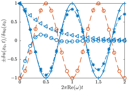
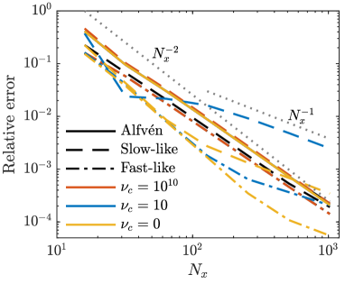
Figure 17: Propagation of oblique linear waves within the Athena++ CGL Landau-fluid implementation in one spatial dimension. Background parameters are $p_{\perp}=p_{\|}=5$, $\rho=1$, $\bm{u}_{0}=0$, and $\bm{B}_{0}=(1,\sqrt{2},0.5)$, with $\bm{k}=2\pi\hat{\bm{x}}$ and $k_{L}=|\bm{k}|$. The left panel shows the time evolution of $\rho u_{y}(x_{m},t)$, where $x_{m}$ is chosen so that $\rho u_{y}(x_{m},0)$ is the maximum of the sinusoidal initial condition. Results are normalised to the initial amplitude of ${\simeq}10^{-4}$. The curves show the expected linear solution, computed analytically from the dispersion relation (42)–(44), while symbols show results from Athena++ with $N_{x}=1024$. Blue lines/symbols show $\nu_{\rm c}=10$, with the solid line (plus symbols), dashed line (circle symbols), dot-dashed line (star symbols), and dotted line (triangle symbols) corresponding to the Alfvén, slow-like, fast-like, and entropy-like modes, respectively. The red dashed curve (circle symbols) shows the slow mode at $\nu_{\rm c}=10^{10}$ to illustrate how the system reverts to undamped adiabatic MHD at high $\nu_{\rm c}$. The right panel shows the normalised root-mean-squared error in the solution, as measured from the analytic solution, as a function of spatial resolution $N_{x}$. Line styles and colours are as in the left panel, with the addition of yellow curves for collisionless modes ($\nu_{\rm c}=0$) and black for pure CGL (no heat fluxes; $k_{L}\rightarrow\infty$). We see almost second-order convergence for most solutions, except for those that are dominated by damping from heat fluxes, in particular the collisionless/weakly collisional slow mode (blue and yellow dashed lines; the former is overdamped $|{\rm Im}(\omega)|>|{\rm Re}(\omega)|$, see left-hand panel).

Code testing was carried out with standard problems and methods, such as examining the total-energy conservation, nonlinear Alfvén-wave dynamics (Squire et al., 2016), and linear waves. Figure 17 illustrates the ability of the solver to capture the diverse linear behaviour of the CGL-LF system. The tests involve initialising the solver with a chosen linear eigenmode, computed analytically from the linearised system, then comparing the frequency and decay rate from the code to the analytic expectations. In the right-hand panel, we show the convergence to the analytic solution with spatial resolution for a range of different waves and parameters, scanning from the collisionless system out to the adiabatic-MHD with $\nu_{\rm c}=10^{10}$. For modes that are only weakly damped, meaning their dynamics are dominated by the conservative (CGL) solver, we see almost second-order convergence. With more strongly damped modes, for which the error becomes dominated by the non-conservative heat flux and/or collisions in the solver, we see first-order convergence above some resolution that depends on the mode in question (this behaviour is clearest for the slow-like modes shown with dashed lines, because these are more strongly damped).

A.3 Numerical problems and challenges

The CGL system seems to be particularly prone to numerical instability, which hampered efforts to design more accurate numerical solvers. As part of the code development effort for this work, we tested a wide variety of different numerical options and solvers, all of which showed some issues in certain situations. Our final choice of the piecewise parabolic method with an HLL Reimman solver and the conserved variable $\mathcal{A}$ (see 39) was made by trading off the various issues that arose in different numerical tests. Examples include a pernicious numerical instability that acts on the compressive components of the system at the smallest scales, creating flute-like ($k_{\perp}\gg k_{\|}$) grid-scale modes that can grow sufficiently to break up wave solutions in certain circumstances; or virulent numerical instabilities that arise in regions of small $|\bm{B}|$ when $\mu$ rather than $\mathcal{A}$ is used as the conserved variable. While we do not fully understand the root causes of these issues, we speculate that they may be worse than standard in MHD because the system involves two different volumetrically conserved variables ($\rho$ and $\mu$ or $\mathcal{A}$) that feed back on the momentum in different ways.

As part of this development process, we designed a new Riemann solver for the CGL system that treats the Alfvénic-branch solutions separately, just like the popular HLLD solver for MHD (Miyoshi & Kusano, 2005; Mignone, 2007). This has significantly improved accuracy for problems involving predominantly Alfvénic fluctuations. Although this made it an obvious candidate for our Alfvénic turbulence simulations, the solver was ultimately found to cause issues in our higher-resolution turbulence simulations, even though it worked quite well for many simpler test problems. This type of behaviour is not uncommon, for example, also occurring in HLLC and related hydrodynamic finite-volume solvers, which can suffer from serious numerical issues if shocks develop (see, e.g., Simon & Mandal, 2019, and references therein). For this reason, for our main simulations, we reverted back to the simplest HLL solver, using parabolic reconstruction to reduce the large numerical dissipation that is inherent to this method. Nonetheless, in case the HLLD solver proves useful for other problems in future works, we provide a brief description of it below.

A.3.1 An HLLD CGL Riemann solver

Rather than proceeding in the most obvious way, by extending the HLLD method of Miyoshi & Kusano (2005) to the double-adiabatic mode structure, we instead base our solver on the isothermal HLLD solver of Mignone (2007). The method thus computes the fluxes of thermodynamic variables using the simple HLL method (Harten et al., 1983), while those of the transverse momentum and magnetic field are obtained using a more accurate computation of the wave structure. It enables shear-Alfvénic dynamics (or rotational discontinuities) to be captured accurately, while avoiding various very complex and time-consuming nonlinear solves that arise if one attempts to replicate the method of Miyoshi & Kusano (2005).

The basis for the solver is to take $\rho$, $m_{x}$, $E$, $\mathcal{A}$, and their fluxes as constant across the Riemann fan. In contrast, the ‘Alfvénic variables’, $m_{y}$, $m_{z}$, $B_{y}$, and $B_{z}$, are allowed to vary across the fan, being separated into three states $\bm{U}_{L}^{*}$, $\bm{U}_{c}^{*}$, and $\bm{U}_{R}^{*}$ by the left and right Alfvén discontinuities with velocities $S^{*}_{L}$ and $S^{*}_{R}$, as in isothermal MHD (Mignone, 2007). We then use the consistency conditions for a five-state Riemann solver separated by waves $S_{L}$, $S_{L}^{*}$, $S_{R}^{*}$, and $S_{R}$ (Mignone, 2007; Toro, 2009):

$$\frac{(S_{L}^{*}-S_{L})\bm{U}^{*}_{L}+(S_{R}^{*}-S_{L}^{*})\bm{U}^{*}_{c}+(S_{R}-S_{R}^{*})\bm{U}^{*}_{R}}{S_{R}-S_{L}}=\bm{U}^{\rm hll},$$ (45)

for the conserved variables $\bm{U}$, and

$$\frac{(S_{L}^{*-1}-S_{L}^{-1})\bm{F}^{*}_{L}+(S_{R}^{*-1}-S_{L}^{*-1})\bm{F}^{*}_{c}+(S_{R}^{-1}-S_{R}^{*-1})\bm{F}^{*}_{R}}{S_{R}^{-1}-S_{L}^{-1}}=\bm{F}^{\rm hll}$$ (46)

for the fluxes $\bm{F}$. Here $\bm{U}^{\rm hll}$ and $\bm{F}^{\rm hll}$ are the HLLE states and fluxes:

$$\bm{U}^{\rm hll}\doteq\frac{S_{R}\bm{U}_{R}-S_{L}\bm{U}_{L}-\bm{F}_{R}+\bm{F}_{L}}{S_{R}-S_{L}},$$ (47)

$$\bm{F}^{\rm hll}\doteq\frac{S_{R}^{-1}\bm{F}_{R}-S_{L}^{-1}\bm{F}_{L}-\bm{U}_{R}+\bm{U}_{L}}{S_{R}^{-1}-S_{L}^{-1}}.$$ (48)

Applying the assumption $\bm{U}_{L}^{*}=\bm{U}_{c}^{*}=\bm{U}_{R}^{*}=\bm{U}^{*}$ to the non-Alfvénic variables gives $\bm{U}^{*}=\bm{U}^{\rm hll}$, $\bm{F}^{*}=\bm{F}^{\rm hll}$, as expected. It remains to determine $\bm{U}_{L}^{*}$, $\bm{U}_{R}^{*}$, and their fluxes for the Alfvénic variables, after which $\bm{F}_{c}^{*}$ is determined from 46.

We compute the jump conditions for the Alfvénic variables across the $S_{L}$ and $S_{R}$ waves following Mignone (2007):

$$\bm{F}^{*}_{L}=\bm{F}_{L}+S_{L}(\bm{U}_{L}-\bm{U}_{L}^{*}),$$ (49)

$$\bm{F}^{*}_{R}=\bm{F}_{R}+S_{R}(\bm{U}_{R}-\bm{U}_{R}^{*}).$$ (50)

This leads to

$$\rho^{*}u_{y\alpha}^{*}=\rho^{*}u_{y\alpha}-B_{x}B_{y\alpha}\frac{u_{x}^{*}\Uptheta_{\alpha}-u_{x\alpha}\Uptheta^{*}+S_{\alpha}(\Uptheta^{*}-\Uptheta_{\alpha})}{(S_{\alpha}-S_{L}^{*})(S_{\alpha}-S_{R}^{*})},$$ (51)

$$\rho^{*}u_{z\alpha}^{*}=\rho^{*}u_{z\alpha}-B_{x}B_{z\alpha}\frac{u_{x}^{*}\Uptheta_{\alpha}-u_{x\alpha}\Uptheta^{*}+S_{\alpha}(\Uptheta^{*}-\Uptheta_{\alpha})}{(S_{\alpha}-S_{L}^{*})(S_{\alpha}-S_{R}^{*})},$$ (52)

$$B_{y\alpha}^{*}=\frac{B_{y\alpha}}{\rho^{*}}\frac{\rho_{\alpha}(S_{\alpha}-u_{\alpha})^{2}-B_{x}^{2}\Uptheta_{\alpha}}{(S_{\alpha}-S_{L}^{*})(S_{\alpha}-S_{R}^{*})},$$ (53)

$$B_{z\alpha}^{*}=\frac{B_{z\alpha}}{\rho^{*}}\frac{\rho_{\alpha}(S_{\alpha}-u_{\alpha})^{2}-B_{x}^{2}\Uptheta_{\alpha}}{(S_{\alpha}-S_{L}^{*})(S_{\alpha}-S_{R}^{*})}.$$ (54)

Here $\alpha$ denotes either $L$ or $R$, $\rho^{*}=\rho^{\rm hll}$, $u_{x}^{*}=F_{\rho}^{\rm hll}/\rho^{\rm hll}$, and $\Uptheta^{*}$ is the anisotropy parameter ($\Uptheta\doteq 1+\Delta p/B^{2}$) across the fan (see below). The Alfvénic wave speeds, $S_{L,R}^{*}$, are

$$S_{L}^{*}=u_{x}^{*}-\sqrt{\frac{\Uptheta^{*}}{\rho^{*}}}|B_{x}|,\quad S_{R}^{*}=u_{x}^{*}+\sqrt{\frac{\Uptheta^{*}}{\rho^{*}}}|B_{x}|.$$ (55)

These are fixed by the jump conditions from the left and right regions to the central regions after asserting that $\Uptheta^{*}$ should be constant (this is in keeping with the assumption that only Alfvénic quantities change inside the fan; see equations (25)–(28) of Mignone 2007). The numerical flux is then computed as

$$\bm{F}=\begin{cases}\bm{F}_{L},&0<S_{L},\\ \bm{F}_{L}^{*},&S_{L}<0<S_{L}^{*},\\ \bm{F}_{c}^{*},&S_{L}^{*}<0<S_{R}^{*},\\ \bm{F}_{R}^{*},&S_{R}^{*}<0<S_{R},\\ \bm{F}_{R},&S_{R}<0,\end{cases}$$ (56)

where $\bm{F}_{L}^{*}$ and $\bm{F}_{R}^{*}$ are computed from 49 and 50, and $\bm{F}_{c}^{*}$ from the consistency condition (46).

The firehose parameter $\Uptheta^{*}$ remains unspecified. Unfortunately, it is not possible to have $\Delta p/B^{2}$, $E$, and $\mathcal{A}$ all constant across the central region for general $B_{y}$ and $B_{z}$ that vary as in 53 and 54. We are thus forced to consider $B^{2}$ in $\Uptheta$ to be some average across the fan. There appears to be no way to circumvent this inconsistency, so long as we assume that non-Alfvénic variables are constant across then fan, while Alfvénic components vary. We are thus left with choosing a suitable average for defining $\Uptheta^{*}$. We have experimented with various possibilities for doing this, finding that the most robust method seems to be to use the HLL average to compute $B^{2}$ (i.e., using $B_{y}^{\rm hll}$ and $B_{z}^{\rm hll}$). This method has the advantage of being straightforward and fast to execute, while also being conceptually consistent with the idea that non-Alfvénic variables ($B^{2}$ in this case) should be computed using HLL averages.

Special cases. There are two special cases that must be dealt with in the solver. The first, which occurs if $S_{\alpha}^{*}\rightarrow S_{\alpha}$, is handled identically to the Mignone (2007) solver by imposing a zero jump across $m_{y}$, $m_{z}$, $B_{y}$, and $B_{z}$. As in isothermal MHD, there is no issue with the limit $B_{x}\rightarrow 0$, which simply leads to $S_{\alpha}^{*}=u^{*}$ and various simplifications of (51)–(54).

The other special case occurs as $\Uptheta$ approaches 0. For $\Uptheta<0$, Alfvén waves are unstable, and it no longer makes sense to compute the wave structure in the same way. We thus switch to a standard HLL solver for all variables if $\Uptheta_{L}$, $\Uptheta^{*}$, or $\Uptheta_{R}$ is below some threshold $\Uptheta_{\mathrm{thresh}}$. In practice, $\Uptheta_{\mathrm{thresh}}\approx 0.1$ seems to give reasonable results (recall that Alfvénic perturbations propagate very slowly for small $\Uptheta$ anyway). The switch to the HLL solver is carried out using the ‘anti-diffusion control’ method described presently.

Anti-diffusion control. As mentioned above, the CGL HLLD method displayed numerical instabilities, in particular small-scale oscillations in $\Uptheta$, which became worse for more complex problems. These can often be mitigated by the ‘anti-diffusion control’ method of Simon & Mandal (2019), which was proposed to solve the ‘Carbuncle’ problem of the hydrodynamic HLLC solver. The method involves continuously switching to the more diffusive HLL solver at the advent of grid-scale oscillations. It is derived by rewriting 49 and 50 as

$$\bm{F}^{*}_{L}=\bm{F}^{\rm hll}+S_{L}(\bm{U}^{\rm hll}-\bm{U}_{L}^{*}),$$ (57)

$$\bm{F}^{*}_{R}=\bm{F}^{\rm hll}+S_{R}(\bm{U}^{\rm hll}-\bm{U}_{R}^{*}),$$ (58)

then recognising the second term on each right-hand side as an ‘anti-diffusive’ contribution to the flux (it corrects the HLL flux, making it less diffusive). Multiplying this contribution by a factor $\omega_{\mathrm{AD}}$ satisfying $0\leq\omega_{\mathrm{AD}}\leq 1$, gives a method to interpolate between the HLLD and HLL solvers. As a simple option, $\omega_{\mathrm{AD}}$ can be chosen as $\omega_{\mathrm{AD}}=\exp(-\alpha_{\mathrm{AD}}\max|\Delta\Uptheta|)$, where $\max|\Delta\Uptheta|$ is the maximum value of $|\Uptheta_{L}-\Uptheta_{R}|$ across the interface and its two neighbors perpendicular to the interface. The free parameter $\alpha_{\mathrm{AD}}$ controls the strength of the anti-diffusive effect, with $\alpha_{\mathrm{AD}}\approx 10$ providing a reasonable trade off between accuracy and stability for a range of parameters and problems. We also multiply $\omega_{\mathrm{AD}}$ by $H(\Uptheta_{\mathrm{min}}-\Uptheta_{\mathrm{thresh}})$, where $H(x)$ is the Heaviside step function and $\Uptheta_{\mathrm{min}}=\min\{\Uptheta_{L},\Uptheta^{*},\Uptheta_{R}\}$, to switch to the HLL solver as the system approaches the firehose instability condition (see above). More information and stability analysis of the anti-diffusion control method in the HLLC context can be found in Simon & Mandal (2019).

References

- Arzamasskiy et al. (2019) Arzamasskiy, L., Kunz, M. W., Chandran, B. D. G. & Quataert, E. 2019 Hybrid-kinetic simulations of ion heating in Alfvénic turbulence. Astrophys. J. 879, 53.
- Arzamasskiy et al. (2023) Arzamasskiy, L., Kunz, M. W., Squire, J., Quataert, E. & Schekochihin, A. A. 2023 Kinetic turbulence in collisionless high- plasmas. Phys. Rev. X 13, 021014.
- Bale et al. (2009) Bale, S. D., Kasper, J. C., Howes, G. G., Quataert, E., Salem, C. & Sundkvist, D. 2009 Magnetic fluctuation power near proton temperature anisotropy instability thresholds in the solar wind. Phys. Rev. Lett. 103, 211101.
- Baranov (1970) Baranov, V. B. 1970 Simple waves in a plasma with anisotropic pressure. Fluid Dynamics 5, 181.
- Barnes (1966) Barnes, A. 1966 Collisionless damping of hydromagnetic waves. Phys. Fluids 9, 1483.
- Barnes & Hollweg (1974) Barnes, A. & Hollweg, J. V. 1974 Large-amplitude hydromagnetic waves. J. Geophys. Res. 79, 2302.
- Belcher & Davis (1971) Belcher, J. W. & Davis, Leverett, J. 1971 Large-amplitude Alfvén waves in the interplanetary medium, 2. J. Geophys. Res. 76, 3534.
- Boldyrev (2006) Boldyrev, S. 2006 Spectrum of magnetohydrodynamic turbulence. Phys. Rev. Lett. 96, 115002.
- Borovsky & Valdivia (2018) Borovsky, J. E. & Valdivia, J. A. 2018 The Earth’s magnetosphere: A systems science overview and assessment. Surveys in Geophys. 39, 817.
- Bott et al. (2021) Bott, A. F. A., Arzamasskiy, L., Kunz, M. W., Quataert, E. & Squire, J. 2021 Adaptive critical balance and firehose instability in an expanding, turbulent, collisionless plasma. Astrophys. J. Lett. 922, L35.
- Braginskii (1965) Braginskii, S. I. 1965 Transport processes in a plasma. Rev. Plasma Phys. 1, 205.
- Brandenburg & Subramanian (2005) Brandenburg, A. & Subramanian, K. 2005 Astrophysical magnetic fields and nonlinear dynamo theory. Phys. Rep. 417 1.
- Chandran et al. (2010) Chandran, B. D. G., Li, B., Rogers, B. N., Quataert, E. & Germaschewski, K. 2010 Perpendicular Ion Heating by Low-frequency Alfvén-wave Turbulence in the Solar Wind. Astrophys. J. 720, 503.
- Chandrasekhar et al. (1958) Chandrasekhar, S., Kaufman, A. N. & Watson, K. M. 1958 The stability of the pinch. Proc. R. Soc. A 245, 435–455.
- Chen (2016) Chen, C. H. K. 2016 Recent progress in astrophysical plasma turbulence from solar wind observations. J. Plasma Phys. 82, 535820602.
- Chen et al. (2020) Chen, C. H. K., Bale, S. D., Bonnell, J. W., Borovikov, D., Bowen, T. A., Burgess, D., Case, A. W., Chandran, B. D. G., de Wit, T. D., Goetz, K., Harvey, P. R., Kasper, J. C., Klein, K. G., Korreck, K. E., Larson, D., Livi, R., MacDowall, R. J., Malaspina, D. M., Mallet, A., McManus, M. D., Moncuquet, M., Pulupa, M., Stevens, M. L. & Whittlesey, P. 2020 The evolution and role of solar wind turbulence in the inner heliosphere. Astrophys. J. Supp. 246, 53.
- Chen et al. (2013) Chen, C. H. K., Bale, S. D., Salem, C. S. & Maruca, B. A. 2013 Residual energy spectrum of solar wind turbulence. Astrophys. J. 770, 125.
- Chen et al. (2021) Chen, C. H. K., Chandran, B. D. G., Woodham, L. D., Jones, S. I., Perez, J. C., Bourouaine, S., Bowen, T. A., Klein, K. G., Moncuquet, M., Kasper, J. C. & Bale, S. D. 2021 The near-Sun streamer belt solar wind: turbulence and solar wind acceleration. Astron. Astro. 650, L3.
- Chen et al. (2012) Chen, C. H. K., Mallet, A., Schekochihin, A. A., Horbury, T. S., Wicks, R. T. & Bale, S. D. 2012 Three-dimensional structure of solar wind turbulence. Astrophys. J. 758, 120.
- Chen et al. (2016) Chen, C. H. K., Matteini, L., Schekochihin, A. A., Stevens, M. L., Salem, C. S., Maruca, B. A., Kunz, M. W. & Bale, S. D. 2016 Multi-species measurements of the firehose and mirror instability thresholds in the solar wind. Astrophys. J. 825, 1.
- Chew et al. (1956) Chew, C. F., Goldberger, M. L. & Low, F. E. 1956 The Boltzmann equation and the one-fluid hydromagnetic equations in the absence of particle collisions. Proc. R. Soc. London A 236, 112.
- Cho & Lazarian (2009) Cho, J. & Lazarian, A. 2009 Simulations of electron magnetohydrodynamic turbulence. Astrophys. J. 701, 236.
- Churazov et al. (2004) Churazov, E., Forman, W., Jones, C., Sunyaev, R. & Böhringer, H. 2004 XMM-Newton observations of the Perseus cluster - II. Evidence for gas motions in the core. Mon. Not. R. Astron. Soc. 347, 29.
- Coburn et al. (2022) Coburn, J. T., Chen, C. H. K. & Squire, J. 2022 A measurement of the effective mean free path of solar wind protons. J. Plasma Phys. 88, 175880502.
- Cohen et al. (2017) Cohen, R., Gerrard, A. J., Lanzerotti, L. J., Soto-Chavez, A. R., Kim, H. & Manweiler, J. W. 2017 Climatology of high- plasma measurements in Earth’s inner magnetosphere. J. Geophys. Res. Space Phys. 122, 711.
- Cowie & McKee (1977) Cowie, L. L. & McKee, C. F. 1977 The evaporation of spherical clouds in a hot gas. I - Classical and saturated mass loss rates. Astrophys. J. 211, 135.
- Cox (2005) Cox, D. P. 2005 The three-phase interstellar medium revisited. Ann. Rev. Astron. Astrophys. 43, 337.
- Dong & Stone (2009) Dong, R. & Stone, J. M. 2009 Buoyant bubbles in intracluster gas: Effects of magnetic fields and anisotropic viscosity. Astrophys. J. 704, 1309.
- Dunn et al. (2023) Dunn, C., Bowen, T., Mallet, A., Badman, S. & Bale, S. 2023 Effect of spherical polarization on the magnetic spectrum of the solar wind. arXiv e-prints p. arXiv:2305.09763.
- EHT Collaboration et al. (2019) EHT Collaboration et al. 2019 First M87 event horizon telescope results. i. The shadow of the supermassive black hole. Astrophys. J. Lett. 875, L1.
- Fabian (1994) Fabian, A. C. 1994 Cooling flows in clusters of galaxies. Ann. Rev. Astron. Astrophys. 32, 277.
- Finelli et al. (2021) Finelli, F., Cerri, S. S., Califano, F., Pucci, F., Laveder, D., Lapenta, G. & Passot, T. 2021 Bridging hybrid- and full-kinetic models with Landau-fluid electrons. I. 2D magnetic reconnection. Astron. Astro. 653, A156.
- Foote & Kulsrud (1979) Foote, E. A. & Kulsrud, R. M. 1979 Hydromagnetic waves in high beta plasmas. Astrophys. J. 233, 302.
- Gary & Nishimura (2003) Gary, S. P. & Nishimura, K. 2003 Resonant electron firehose instability: Particle-in-cell simulations. Phys. Plasmas 10, 3571.
- Goldreich & Sridhar (1995) Goldreich, P. & Sridhar, S. 1995 Toward a theory of interstellar turbulence. Strong Alfvénic turbulence. Astrophys. J. 438, 763.
- Grete et al. (2017) Grete, P., O’Shea, B. W., Beckwith, K., Schmidt, W. & Christlieb, A. 2017 Energy transfer in compressible magnetohydrodynamic turbulence. Phys. Plasmas 24, 092311.
- Gross & Krook (1956) Gross, E. P. & Krook, M. 1956 odel for collision processes in gases: Small-amplitude oscillations of charged two-component systems. Phys. Rev. 102, 593.
- Hammett & Perkins (1990) Hammett, G. W. & Perkins, F. W. 1990 Fluid moment models for Landau damping with application to the ion-temperature-gradient instability. Phys. Rev. Lett. 64, 3019.
- Harten et al. (1983) Harten, A., Lax, P. & Leer, B. 1983 On upstream differencing and Godunov-type schemes for hyperbolic conservation laws. SIAM Review 25, 35.
- Hasegawa (1969) Hasegawa, A. 1969 Drift mirror instability of the magnetosphere. Phys. Fluids 12, 2642.
- Hellinger et al. (2011) Hellinger, P., Matteini, L., Štverák, Š., Trávníček, P. M. & Marsch, E. 2011 Heating and cooling of protons in the fast solar wind between 0.3 and 1 AU: Helios revisited. J. Geophys. Res. Space Phys. 116, A09105.
- Hellinger et al. (2006) Hellinger, P., Trávníček, P., Kasper, J. C. & Lazarus, A. J. 2006 Solar wind proton temperature anisotropy: Linear theory and wind/swe observations. Geophysical Research Letters 33, L09101.
- Hellinger & Trávníček (2008) Hellinger, P. & Trávníček, P. M. 2008 Oblique proton fire hose instability in the expanding solar wind: Hybrid simulations. J. Geophys. Res. Space Phys. 113, A10109.
- Hollweg (1971) Hollweg, J. V. 1971 Nonlinear Landau damping of Alfvén waves. Phys. Rev. Lett. 27, 1349.
- Hollweg (1974a) Hollweg, J. V. 1974a On electron heat conduction in the solar wind. J. Geophys. Res. 79 (25), 3845.
- Hollweg (1974b) Hollweg, J. V. 1974b Transverse Alfvén waves in the solar wind: Arbitrary , , , and . J. Geophys. Res. 79, 1539.
- Howes (2010) Howes, G. G. 2010 A prescription for the turbulent heating of astrophysical plasmas. Mon. Not. R. Astron. Soc. 409, L104.
- Howes et al. (2008) Howes, G. G., Cowley, S. C., Dorland, W., Hammett, G. W., Quataert, E. & Schekochihin, A. A. 2008 A model of turbulence in magnetized plasmas: Implications for the dissipation range in the solar wind. J. Geophys. Res. Space Phys. 113, A05103.
- Howes et al. (2006) Howes, G. G., Cowley, S. C., Dorland, W., Hammett, G. W., Quataert, E. & Schekochihin, A. e. A. 2006 Astrophysical gyrokinetics: Basic equations and linear theory. Astrophys. J. 651, 590.
- Hunana et al. (2019) Hunana, P., Tenerani, A., Zank, G. P., Khomenko, E., Goldstein, M. L., Webb, G. M., Cally, P. S., Collados, M., Velli, M. & Adhikari, L. 2019 An introductory guide to fluid models with anisotropic temperatures. Part 1. CGL description and collisionless fluid hierarchy. J. Plasma Phys. 85, 205850602.
- Johnston et al. (2022) Johnston, Z., Squire, J., Mallet, A. & Meyrand, R. 2022 On the properties of Alfvénic switchbacks in the expanding solar wind: Three-dimensional numerical simulations. Phys. Plasmas 29, 072902.
- Kasper et al. (2019) Kasper, J. C., Bale, S. D., Belcher, J. W., Berthomier, M., Case, A. W., Chandran, B. D. G., Curtis, D. W., Gallagher, D., Gary, S. P., Golub, L., Halekas, J. S. et al. 2019 Alfvénic velocity spikes and rotational flows in the near-Sun solar wind. Nature 576, 228.
- Kasper et al. (2002) Kasper, J. C., Lazarus, A. J. & Gary, S. P. 2002 Wind/SWE observations of firehose constraint on solar wind proton temperature anisotropy. Geophys. Res. Lett. 29, 1839.
- Kawazura et al. (2019) Kawazura, Y., Barnes, M. & Schekochihin, A. A. 2019 Thermal disequilibration of ions and electrons by collisionless plasma turbulence. Proc. Nat. Acad. Sci. 116, 771.
- Kawazura et al. (2020) Kawazura, Y., Schekochihin, A. A., Barnes, M., TenBarge, J. M., Tong, Y., Klein, K. G. & Dorland, W. 2020 Ion versus Electron Heating in Compressively Driven Astrophysical Gyrokinetic Turbulence. Phys. Rev. X 10, 041050.
- Kempski et al. (2019) Kempski, P., Quataert, E., Squire, J. & Kunz, M. W. 2019 Shearing-box simulations of MRI-driven turbulence in weakly collisional accretion discs. Mon. Not. R. Astron. Soc. 486, 4013.
- Klein & Spence (2021) Klein, K. & Spence, H. 2021 Helioswarm: Leveraging multi-point, multi-scale spacecraft observations to characterize turbulence. In EGU General Assembly Conference Abstracts, pp. EGU21–6812.
- Kulsrud (1983) Kulsrud, R. M. 1983 MHD description of plasma. In Handbook of Plasma Physics (ed. R N Sagdeev & M N Rosenbluth). Princeton University Press.
- Kunz et al. (2018) Kunz, M. W., Abel, I. G., Klein, K. G. & Schekochihin, A. A. 2018 Astrophysical gyrokinetics: turbulence in pressure-anisotropic plasmas at ion scales and beyond. J. Plasma Phys. 84, 715840201.
- Kunz et al. (2022) Kunz, M. W., Jones, T. W. & Zhuravleva, I. 2022 Plasma Physics of the Intracluster Medium, pp. 1–42. Singapore: Springer.
- Kunz et al. (2015) Kunz, M. W., Schekochihin, A. A., Chen, C. H. K., Abel, I. G. & Cowley, S. C. 2015 Inertial-range kinetic turbulence in pressure-anisotropic astrophysical plasmas. J. Plasma Phys. 81, 325810501.
- Kunz et al. (2010) Kunz, M. W., Schekochihin, A. A., Cowley, S. C., Binney, J. J. & Sanders, J. S. 2010 A thermally stable heating mechanism for the intracluster medium: turbulence, magnetic fields and plasma instabilities. Mon. Not. R. Astron. Soc. 410, 2446.
- Kunz et al. (2014) Kunz, M. W., Schekochihin, A. A. & Stone, J. M. 2014 Firehose and mirror instabilities in a collisionless shearing plasma. Phys. Rev. Lett. 112, 205003.
- Kunz et al. (2020) Kunz, M. W., Squire, J., Schekochihin, A. A. & Quataert, E. 2020 Self-sustaining sound in collisionless, high- plasma. J. Plasma Phys. 86, 905860603.
- Kunz et al. (2016) Kunz, M. W., Stone, J. M. & Quataert, E. 2016 Magnetorotational turbulence and dynamo in a collisionless plasma. Phys. Rev. Lett. 117, 235101.
- Ley et al. (2023) Ley, F., Zweibel, E. G., Riquelme, M., Sironi, L., Miller, D. & Tran, A. 2023 A heating mechanism via magnetic pumping in the intracluster medium. Astrophys. J. 947, 89.
- Li et al. (2020) Li, Y., Gendron-Marsolais, M.-L., Zhuravleva, I., Xu, S., Simionescu, A., Tremblay, G. R., Lochhaas, C., Bryan, G. L., Quataert, E., Murray, N. W., Boselli, A., Hlavacek-Larrondo, J., Zheng, Y., Fossati, M., Li, M., Emsellem, E., Sarzi, M., Arzamasskiy, L. & Vishniac, E. T. 2020 Direct detection of black hole-driven turbulence in the centers of galaxy clusters. Astrophys. J. Lett. 889, L1.
- Lithwick & Goldreich (2001) Lithwick, Y. & Goldreich, P. 2001 Compressible magnetohydrodynamic turbulence in interstellar plasmas. Astrophys. J. 562, 279.
- Lovejoy & Schertzer (2012) Lovejoy, S. & Schertzer, D. 2012 Haar wavelets, fluctuations and structure functions: convenient choices for geophysics. Nonlinear Proc. Geophys. 19, 513.
- Lynn et al. (2012) Lynn, J. W., Parrish, I. J., Quataert, E. & Chandran, B. D. G. 2012 Resonance broadening and heating of charged particles in magnetohydrodynamic turbulence. Astrophys. J. 758, 78.
- Majeski et al. (2023) Majeski, S., Kunz, M. & Squire, J. 2023 Microphysically modified magnetosonic modes in collisionless, high- plasmas. J. Plasma Phys. 89, 905890303.
- Mallet et al. (2015) Mallet, A., Schekochihin, A. A. & Chandran, B. D. G. 2015 Refined critical balance in strong Alfvenic turbulence. Mon. Not. R. Astron. Soc. 449, L77.
- Mallet et al. (2021) Mallet, A., Squire, J., Chandran, B. D. G., Bowen, T. & Bale, S. D. 2021 Evolution of large-amplitude Alfvén waves and generation of switchbacks in the expanding solar wind. Astrophys. J. 918, 62.
- Marsch (2006) Marsch, E. 2006 Kinetic physics of the solar corona and solar wind. Living Rev. Solar Phys. 3, 1.
- Melville et al. (2016) Melville, S., Schekochihin, A. A. & Kunz, M. W. 2016 Pressure-anisotropy-driven microturbulence and magnetic-field evolution in shearing, collisionless plasma. Mon. Not. R. Astron. Soc. 459, 2701.
- Meng et al. (2012) Meng, X., Tóth, G., Sokolov, I. V. & Gombosi, T. I. 2012 Classical and semirelativistic magnetohydrodynamics with anisotropic ion pressure. J. Comp. Phys. 231, 3610.
- Meyer et al. (2014) Meyer, C. D., Balsara, D. S. & Aslam, T. D. 2014 A stabilized Runge-Kutta-Legendre method for explicit super-time-stepping of parabolic and mixed equations. J. Comp. Phys. 257, 594.
- Meyrand et al. (2019) Meyrand, R., Kanekar, A., Dorland, W. & Schekochihin, A. A. 2019 Fluidization of collisionless plasma turbulence. Proc. Nat. Acad. Sci. 116, 1185.
- Meyrand et al. (2021) Meyrand, R., Squire, J., Schekochihin, A. A. & Dorland, W. 2021 On the violation of the zeroth law of turbulence in space plasmas. J. Plasma Phys. 87, 535870301.
- Mignone (2007) Mignone, A. 2007 A simple and accurate Riemann solver for isothermal MHD. J. Comp. Phys. 225, 1427.
- Mikhailovskii & Tsypin (1971) Mikhailovskii, A. B. & Tsypin, V. S. 1971 Transport equations and gradient instabilities in a high pressure collisional plasma. Plasma Phys. 13, 785.
- Miyoshi & Kusano (2005) Miyoshi, T. & Kusano, K. 2005 A multi-state HLL approximate Riemann solver for ideal magnetohydrodynamics. J. Comp. Phys. 208, 315.
- Müller & Grappin (2005) Müller, W. & Grappin, R. 2005 Spectral energy dynamics in magnetohydrodynamic turbulence. Phys. Rev. Lett. 95, 114502.
- Nocera et al. (1986) Nocera, L., Priest, E. R. & Hollweg, J. V. 1986 Nonlinear development of phase-mixed Alfvén waves. Geophys. Astrophys. Fluid Dyn. 35, 111.
- Pan & Johnsen (2017) Pan, S. & Johnsen, E. 2017 The role of bulk viscosity on the decay of compressible, homogeneous, isotropic turbulence. J. Fluid Mech. 833, 717.
- Parashar et al. (2018) Parashar, T. N., Matthaeus, W. H. & Shay, M. A. 2018 Dependence of kinetic plasma turbulence on plasma . Astrophys. J. Lett. 864, L21.
- Parker (1958) Parker, E. N. 1958 Dynamical Instability in an Anisotropic Ionized Gas of Low Density. Phys. Rev. 109, 1874.
- Passot et al. (2014) Passot, T., Henri, P., Laveder, D. & Sulem, P.-L. 2014 Fluid simulations of ion scale plasmas with weakly distorted magnetic fields. FLR-Landau fluid simulations. Europ. Phys. J. D 68, 207.
- Passot et al. (2012) Passot, T., Sulem, P. L. & Hunana, P. 2012 Extending magnetohydrodynamics to the slow dynamics of collisionless plasmas. Phys. Plasmas 19, 082113.
- Peterson & Fabian (2006) Peterson, J. R. & Fabian, A. C. 2006 X-ray spectroscopy of cooling clusters. Phys. Rep. 427, 1.
- Quataert (2001) Quataert, E. 2001 Low radiative-efficiency accretion flows. In Probing the Physics of Active Galactic Nuclei (ed. Bradley M. Peterson, Richard W. Pogge & Ronald S. Polidan), Astronomical Society of the Pacific Conference Series, vol. 224, p. 71.
- Quataert & Gruzinov (1999) Quataert, E. & Gruzinov, A. 1999 Turbulence and particle heating in advection-dominated accretion flows. Astrophys. J. 520, 248.
- Rincon et al. (2015) Rincon, F., Schekochihin, A. A. & Cowley, S. C. 2015 Non-linear mirror instability. Mon. Not. R. Astron. Soc. Lett. 447, L45.
- Riquelme et al. (2015) Riquelme, M. A., Quataert, E. & Verscharen, D. 2015 Particle-in-cell simulations of continuously driven mirror and ion cyclotron instabilities in high beta astrophysical and heliospheric plasmas. Astrophys. J. 800, 27.
- Rosenbluth (1956) Rosenbluth, M. N. 1956 The stability of the pinch. Los Alamos Sci. Lab. Rep. LA-2030.
- Rosin et al. (2011) Rosin, M. S., Schekochihin, A. A., Rincon, F. & Cowley, S. C. 2011 A non-linear theory of the parallel firehose and gyrothermal instabilities in a weakly collisional plasma. Mon. Not. R. Astron. Soc. 413, 7.
- Roy et al. (2022) Roy, S., Bandyopadhyay, R., Yang, Y., Parashar, T. N., Matthaeus, W. H., Adhikari, S., Roytershteyn, V., Chasapis, A., Li, H., Gershman, D. J., Giles, B. L. & Burch, J. L. 2022 Turbulent energy transfer and proton-electron heating in collisionless plasmas. Astrophys. J. 941, 137.
- Russell (2023) Russell, A. J. B. 2023 Nonlinear damping and field-aligned flows of propagating shear Alfvén waves with braginskii viscosity. arXiv e-prints p. arXiv:2303.11128.
- Santos-Lima et al. (2014) Santos-Lima, R., de Gouveia Dal Pino, E. M., Kowal, G., Falceta-Gonçalves, D., Lazarian, A. & Nakwacki, M. S. 2014 Magnetic field amplification and evolution in turbulent collisionless magnetohydrodynamics: An application to the intracluster medium. Astrophys. J. 781, 84.
- Schekochihin (2022) Schekochihin, A. A. 2022 MHD Turbulence: A Biased Review. J. Plasma Phys. 88, 155880501.
- Schekochihin et al. (2009) Schekochihin, A. A., Cowley, S. C., Dorland, W., Hammett, G. W., Howes, G. G., Quataert, E. & Tatsuno, T. 2009 Astrophysical gyrokinetics: Kinetic and fluid turbulent cascades in magnetized weakly collisional plasmas. Astrophys. J. Supp. 182, 310.
- Schekochihin et al. (2005) Schekochihin, A. A., Cowley, S. C., Kulsrud, R. M., Hammett, G. W. & Sharma, P. 2005 Plasma instabilities and magnetic field growth in clusters of galaxies. Astrophys. J. 629, 139.
- Schekochihin et al. (2008) Schekochihin, A. A., Cowley, S. C., Kulsrud, R. M., Rosin, M. S. & Heinemann, T. 2008 Nonlinear growth of firehose and mirror fluctuations in astrophysical plasmas. Phys. Rev. Lett. 100, 081301.
- Sharma & Hammett (2007) Sharma, P. & Hammett, G. W. 2007 Preserving monotonicity in anisotropic diffusion. J. Comp. Phys. 227, 123.
- Sharma & Hammett (2011) Sharma, P. & Hammett, G. W. 2011 A fast semi-implicit method for anisotropic diffusion. J. Comp. Phys. 230, 4899.
- Sharma et al. (2006) Sharma, P., Hammett, G. W., Quataert, E. & Stone, J. M. 2006 Shearing box simulations of the mri in a collisionless plasma. Astrophys. J. 637, 952.
- Sharma et al. (2007) Sharma, P., Quataert, E., Hammett, G. W. & Stone, J. M. 2007 Electron heating in hot accretion flows. Astrophys. J. 667, 714.
- Simon & Mandal (2019) Simon, S. & Mandal, J. C. 2019 A simple cure for numerical shock instability in the HLLC Riemann solver. J. Comp. Phys. 378, 477.
- Sironi & Narayan (2015) Sironi, L. & Narayan, R. 2015 Electron heating by the ion cyclotron instability in collisionless accretion flows. I. Compression-driven instabilities and the electron heating mechanism. Astrophys. J. 800, 88.
- Snyder et al. (1997) Snyder, P. B., Hammett, G. W. & Dorland, W. 1997 Landau fluid models of collisionless magnetohydrodynamics. Phys. Plasmas 4, 3974.
- Squire et al. (2020) Squire, J., Chandran, B. D. G. & Meyrand, R. 2020 In-situ switchback formation in the expanding solar wind. Astrophys. J. Lett. 891, L2.
- Squire et al. (2017b) Squire, J., Kunz, M. W., Quataert, E. & Schekochihin, A. A. 2017 Kinetic simulations of the interruption of large-amplitude shear-Alfvén waves in a high- plasma. Phys. Rev. Lett. 119, 155101.
- Squire et al. (2016) Squire, J., Quataert, E. & Schekochihin, A. A. 2016 A stringent limit on the amplitude of Alfvénic perturbations in high-beta low-collisionality plasmas. Astrophys. J. Lett. 830, L25.
- Squire et al. (2017a) Squire, J., Schekochihin, A. A. & Quataert, E. 2017 Amplitude limits and nonlinear damping of shear-Alfvén waves in high-beta low-collisionality plasmas. New J. Phys. 19, 055005.
- Squire et al. (2019) Squire, J., Schekochihin, A. A., Quataert, E. & Kunz, M. W. 2019 Magneto-immutable turbulence in weakly collisional plasmas. J. Plasma Phys. 85, 905850114.
- St-Onge et al. (2020) St-Onge, D. A., Kunz, M. W., Squire, J. & Schekochihin, A. A. 2020 Fluctuation dynamo in a weakly collisional plasma. J. Plasma Phys. 86, 905860503.
- Stone et al. (2020) Stone, J. M., Tomida, K., White, C. J. & Felker, K. G. 2020 The Athena++ Adaptive Mesh Refinement Framework: Design and Magnetohydrodynamic Solvers. Astrophys. J. Supp. 249, 4.
- Tenerani & Velli (2020) Tenerani, A. & Velli, M. 2020 Alfvénic fluctuations in the solar wind: nonlinearities and pressure anisotropy effects. Plasma Phys. Control. Fusion 62, 014001.
- Toro (2009) Toro, E. 2009 Riemann Solvers and Numerical Methods for Fluid Dynamics: A Practical Introduction. Springer Berlin Heidelberg.
- Tumlinson et al. (2017) Tumlinson, J., Peeples, M. S. & Werk, J. K. 2017 The circumgalactic medium. Ann. Rev. Astron. Astrophys. 55, 389.
- Vaidya et al. (2017) Vaidya, B., Prasad, D., Mignone, A., Sharma, P. & Rickler, L. 2017 Scalable explicit implementation of anisotropic diffusion with Runge-Kutta-Legendre super-time stepping. Mon. Not. R. Astron. Soc. 472, 3147.
- Vasquez & Hollweg (1998) Vasquez, B. J. & Hollweg, J. V. 1998 Formation of spherically polarized Alfvén waves and imbedded rotational discontinuities from a small number of entirely oblique waves. J. Geophys. Res. Space Phys. 103, 335.
- Vedenov & Sagdeev (1958) Vedenov, A. A. & Sagdeev, R. Z. 1958 Sov. Phys. Dokl. 3, 278.
- Verscharen et al. (2022) Verscharen, D., Chandran, B. D. G., Boella, E., Halekas, J., Innocenti, M. E., Jagarlamudi, V. K., Micera, A., Pierrard, V., Štverák, Š., Vasko, I. Y., Velli, M. & Whittlesey, P. L. 2022 Electron-driven instabilities in the solar wind. Front. Astron. Space Sci. 9, 951628.
- Verscharen et al. (2016) Verscharen, D., Chandran, B. D. G., Klein, K. G. & Quataert, E. 2016 Collisionless isotropization of the solar-wind protons by compressive fluctuations and plasma instabilities. Astrophys. J. 831, 128.
- Verscharen et al. (2019) Verscharen, D., Klein, K. G. & Maruca, B. A. 2019 The multi-scale nature of the solar wind. Living Rev. Solar Phys. 16, 5.
- Völk & Aplers (1973) Völk, H. J. & Aplers, W. 1973 The propagation of Alfvén waves and their directional anisotropy in the solar wind. Astrophys. Space Sci. 20, 267.
- White et al. (2016) White, C. J., Stone, J. M. & Gammie, C. F. 2016 An extension of the Athena++ code framework for GRMHD based on advanced riemann solvers and staggered-mesh constrained transport. Astrophys. J. Supp. 225, 22.
- Yang et al. (2017) Yang, Y., Matthaeus, W. H., Parashar, T. N., Haggerty, C. C., Roytershteyn, V., Daughton, W., Wan, M., Shi, Y. & Chen, S. 2017 Energy transfer, pressure tensor, and heating of kinetic plasma. Phys. Plasmas 24, 072306.
- Yang et al. (2022) Yang, Y., Matthaeus, W. H., Roy, S., Roytershteyn, V., Parashar, T. N., Bandyopadhyay, R. & Wan, M. 2022 Pressure-strain interaction as the energy dissipation estimate in collisionless plasma. Astrophys. J. 929, 142.
- Yoon et al. (1993) Yoon, P. H., Wu, C. S. & de Assis, A. S. 1993 Effect of finite ion gyroradius on the fire-hose instability in a high beta plasma. Phys. Fluids B 5, 1971.
- Zhdankin et al. (2021) Zhdankin, V., Uzdensky, D. A. & Kunz, M. W. 2021 Production and persistence of extreme two-temperature plasmas in radiative relativistic turbulence. Astrophys. J. 908, 71.
- Zhuravleva et al. (2019) Zhuravleva, I., Churazov, E., Schekochihin, A. A., Allen, S. W., Vikhlinin, A. & Werner, N. 2019 Suppressed effective viscosity in the bulk intergalactic plasma. Nature Astron. 3, 832.
- Zhuravleva et al. (2014) Zhuravleva, I., Churazov, E., Schekochihin, A. A. et al. 2014 Turbulent heating in galaxy clusters brightest in X-rays. Nature 515, 85.