Near-Field Modelling and Performance Analysis for Extremely Large-Scale IRS Communications

Abstract

Intelligent reflecting surface (IRS) is an emerging technology for wireless communications, thanks to its powerful capability to engineer the radio environment. However, in practice, this benefit is attainable only when the passive IRS is of sufficiently large size, for which the conventional uniform plane wave (UPW)-based far-field model may become invalid. In this paper, we pursue a near-field modelling and performance analysis for wireless communications with extremely large-scale IRS (XL-IRS). By taking into account the directional gain pattern of IRS’s reflecting elements and the variations in signal amplitude across them, we derive both the lower- and upper-bounds of the resulting signal-to-noise ratio (SNR) for the generic uniform planar array (UPA)-based XL-IRS. Our results reveal that, instead of scaling quadratically and unboundedly with the number of reflecting elements $M$ as in the conventional UPW-based model, the SNR under the new non-uniform spherical wave (NUSW)-based model increases with $M$ with a diminishing return and eventually converges to a certain limit. To gain more insights, we further study the special case of uniform linear array (ULA)-based XL-IRS, for which a closed-form SNR expression in terms of the IRS size and locations of the base station (BS) and the user is derived. Our result shows that the SNR is mainly determined by the two geometric angles formed by the BS/user locations with the IRS, as well as the dimension of the IRS. Numerical results validate our analysis and demonstrate the necessity of proper near-field modelling for wireless communications aided by XL-IRS.

I Introduction

With the extensive deployment of the fifth-generation (5G) mobile communication networks, researchers from both industry and academia have started the investigation of beyond 5G (B5G) and sixth-generation (6G) wireless networks [2, 3, 4, 5]. To enhance the key performance metrics by orders-of-magnitude (e.g., data rate, latency, and connectivity density), several promising technologies have emerged, such as extremely large-scale multiple-input multiple-output (XL-MIMO) [6, 7, 8, 9, 10, 11, 12], TeraHertz communication [13, 14], and intelligent reflecting surface (IRS) [15, 16, 17, 18, 19, 20, 21]. In particular, IRS is a promising technology to achieve cost-effective and energy-efficient wireless communication by proactively manipulating the radio propagation environment [20, 21, 18]. Compared with conventional relays, IRS-aided communication dispenses with costly radio frequency (RF) chains and operates in a full-duplex mode, which is thus free of self-interference and noise amplification. However, due to the double path-loss attenuation for signals reflected by IRS, to practically reap the promising performance gain of IRS-aided communications, the physical/electrical size of IRS needs to be sufficiently large[22, 1], leading to communication scenarios with extremely large-scale IRS (XL-IRS). Note that the appealing features of lightweight and conformal geometry render it possible to deploy XL-IRSs in practice, such as on the facades of buildings, indoor walls and ceilings, etc.

Most existing literatures on IRS-aided communications have focused on the conventional far-field uniform plane wave (UPW) assumption for ease of channel modelling and performance analysis, where all of IRS’s reflecting elements share the identical angles of arrival/departure (AoA/AoD) for the same channel path [15, 16, 18, 21]. Note that the typical criterion to separate the far- and near-field propagation region is Rayleigh distance, i.e., $r\geq\frac{2D^{2}}{\lambda}$, where $r$ is the link distance, $D$ and $\lambda$ denote the array physical dimension and signal wavelength, respectively [23, 24, 25, 26, 10]. As the aperture of IRS significantly increases, the transmitter and/or the receiver may no longer be located in the far-field region of XL-IRSs, and the conventional UPW-based signal model may become invalid[1]. Instead, the near-field signal characteristics with the more generic non-uniform spherical wave (NUSW) propagation [27, 28] should be considered to accurately model the variations in received signal amplitude, phase, and AoA/AoD across different reflecting elements of the IRS. There have been several attempts on the mathematical modelling and performance analysis for active antenna array communications under the near-field NUSW model [10, 29]. For instance, in [10], by considering the variations in signal amplitude, phase and projected aperture over different array elements, the authors derived a closed-form expression for the received signal-to-noise ratio (SNR) for XL-MIMO communications. Additionally, the multi-user XL-MIMO communication was investigated in [29] based on three typical beamforming schemes, i.e., the maximal-ratio combining (MRC), zero-forcing (ZF), and minimum mean-square error (MMSE) beamforming. Besides, mathematical model considering the near-field signal characteristics has been studied in the passive array/surface-based communications [30, 31, 32, 33]. For example, in [30], the impacts brought by distance variations in the near-field model were analyzed for the continuous surface, and accurate expressions for the achievable spatial degrees-of-freedom (DoFs) of large intelligent surfaces (LIS)-based communications were derived. In [31], the power scaling laws and near-field behaviors of large-scale IRS were investigated under the two-dimensional (2D) modelling without considering the elevation AoA/AoD. In [32], the asymptotic performance of IRS-aided simultaneous transmit diversity and passive beamforming, with the growing number of reflecting elements, was derived in closed-form by considering the difference in signal amplitude and projected aperture over different reflecting elements. Moreover, a new distance-based metric was provided for accurate characterization of the antenna array gain in [33].

Besides the NUSW-based near-field modelling, another important aspect of analyzing the performance of XL-IRS-aided communications is on accurately modelling the directional gain pattern of each individual reflecting element. Most existing works have modelled each element’s reflection pattern isotropically, which, however, may lead to impractical results that violate the law of power conservation as the IRS size becomes large, i.e., the total received power even exceeds the transmitted power. To tackle this issue, directional gain pattern has been widely considered in antenna theory [19, 34, 35, 36]. Specifically, in [19] and [34], the impact of IRS reflecting element’s directivity was considered in the path loss modelling, which was explicitly expressed as an angle-dependent loss factor and validated by experimental results. In [35], a received power model for an IRS-aided wireless communication system was proposed. It was shown that the received power depends on the effective aperture of individual reflecting element, and then the radar cross section (RCS) was adopted to characterize each element’s directivity. Besides, by following the directional radiation gain pattern commonly used in the active arrays[26], the modelling with directional reflection gain pattern was further considered for IRS-aided communications in [36] and [37]. However, the aforementioned works do not provide a rigorous near-field performance analysis, such as power scaling laws and asymptotic SNR expressions with respect to the number of IRS reflecting elements.

To fill the above gaps, we study in this paper the three-dimensional (3D) near-field modelling and performance analysis for wireless communications aided by XL-IRS. The main contributions of this paper are summarized as follows.

• Firstly, by taking into account the directional gain pattern of IRS’s reflecting elements and the variations in received signal amplitude and AoA/AoD across them, a generic near-field modelling is developed for XL-IRS-aided communications based on the Friis Transmission Equation[38]. Based on the developed model, tight lower- and upper-bounds of the received SNR are derived for the generic uniform planar array (UPA)-based XL-IRS. By further analysis, it is revealed that instead of scaling quadratically and unboundedly with the number of reflecting elements $M$ as in the conventional UPW-based far-field model [16, 21], the SNR under the new NUSW-based near-field model increases with $M$ with a diminishing return and eventually converges to a certain limit.

• Next, to gain further insights into our derived bounds, we also investigate the special case of uniform linear array (ULA)-based XL-IRS, for which a closed-form SNR expression in terms of the IRS size and locations of the base station (BS) and the user is derived. Similar to [9], it is shown that the SNR mainly depends on the two geometric angles formed by the BS/user locations with the IRS, as well as the dimension of the IRS.

• Lastly, the developed model is extended to the multiple-input single-output (MISO) setup, where the BS is equipped with multiple antennas. To comply with the typical deployment strategy where the IRS is deployed closer to either the BS or the user [15, 21], we consider the scenario where the user is located in the near-field region of the IRS while the BS is in the far-field region of it. With the optimal single-user maximum ratio combining/transmission (MRC/MRT) beamforming, an integral form of the received SNR is derived. Furthermore, we derive tight lower- and upper-bounds of the received SNR in closed-form expressions under a special gain pattern. The results reveal that for the MISO scenario, there still exists a notable performance gap between the conventional UPW model and the new near-field model as the IRS size becomes large.

The rest of this paper is organized as follows. Section II introduces the near-field modelling for XL-IRS-aided communications. In Section III, tight lower- and upper-bounds of the SNR expression are derived for the UPA-based XL-IRS, and the special case of ULA-based XL-IRS is also considered. We then extend our developed model to the MISO setup with more insights given in Section IV. Numerical results are provided in Section V. Finally, we conclude our paper in Section VI.

II System Model

As shown in Fig. 1, we consider a wireless communication system, where an XL-IRS is deployed to assist in the communication between the BS and the user. For ease of exposition, we assume that the user is equipped with one antenna, and the IRS is of UPA architecture. The separation between adjacent elements is denoted by $d\leq\frac{\lambda}{2}$, where $\lambda$ denotes the signal wavelength. It is assumed that the XL-IRS is located on the $y$-$z$ plane and centered at the origin, and we have the total number of IRS reflecting elements as $M=M_{y}M_{z}\gg 1$ with $M_{y}$ and $M_{z}$ denoting the number of reflecting elements along the $y$- and $z$-axis, respectively. Based on the above notations, the entire IRS size can be expressed as $L_{y}\times L_{z}$, where $L_{y}\simeq M_{y}d$ and $L_{z}\simeq M_{z}d$.

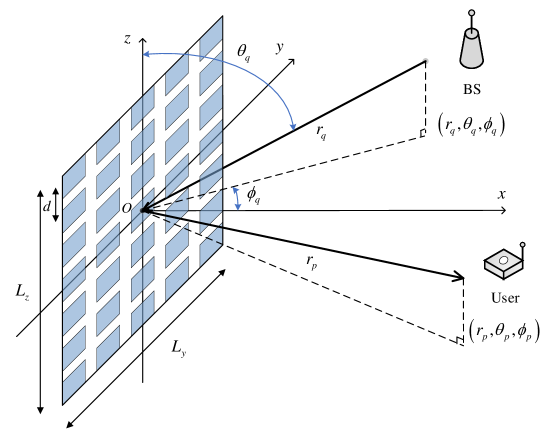
Figure 1: Wireless communication assisted by XL-IRS.

For notational convenience, we assume that both $M_{y}$ and $M_{z}$ are odd numbers. Without loss of generality, a Cartesian coordinate system is established so that the center of the XL-IRS coincides with the origin. The central location of the $\left(m_{y},m_{z}\right)$-th reflecting element is denoted as $\mathbf{w}_{m_{y},m_{z}}=\left[0,m_{y}d,m_{z}d\right]^{T}$, where $m_{y}=0,\pm 1,\cdots,\pm\left(M_{y}-1\right)/2$, $m_{z}=0,\pm 1,\cdots,\pm\left(M_{z}-1\right)/2$. Denote the distance between the BS and the center of the XL-IRS as $r_{q}$, and the location of the BS is then denoted as $\mathbf{q}=\left[r_{q}\Psi_{q},r_{q}\Phi_{q},r_{q}\Theta_{q}\right]^{T}$, with $\Psi_{q}\triangleq\sin\theta_{q}\cos\phi_{q}$, $\Phi_{q}\triangleq\sin\theta_{q}\sin\phi_{q}$, and $\Theta_{q}\triangleq\cos\theta_{q}$, where $\theta_{q}\in\left[0,\pi\right]$ and $\phi_{q}\in\left[-\frac{\pi}{2},\frac{\pi}{2}\right]$ denote the zenith and azimuth angles of the BS, respectively. Thus, the distance between the BS and the $(m_{y},m_{z})$-th reflecting element can be expressed as

$$r_{q,m_{y},m_{z}}=\left\|\mathbf{q}-\mathbf{w}_{m_{y},m_{z}}\right\|=r_{q}\sqrt{1-2m_{y}\varepsilon_{q}\Phi_{q}-2m_{z}\varepsilon_{q}\Theta_{q}+\left(m_{y}^{2}+m_{z}^{2}\right)\varepsilon_{q}^{2}},$$ (1)

where $\varepsilon_{q}\triangleq\frac{d}{r_{q}}$. Note that in practice, we have $\varepsilon_{q}\ll 1$ [10, 1].

Similarly, denote the location of the user as $\mathbf{p}=\left[r_{p}\Psi_{p},r_{p}\Phi_{p},r_{p}\Theta_{p}\right]^{T}$, with $\Psi_{p}\triangleq\sin\theta_{p}\cos\phi_{p}$, $\Phi_{p}\triangleq\sin\theta_{p}\sin\phi_{p}$, and $\Theta_{p}\triangleq\cos\theta_{p}$, where $r_{p}$ is the distance between the XL-IRS center and the user, and $\theta_{p}\in\left[0,\pi\right]$ and $\phi_{p}\in\left[-\frac{\pi}{2},\frac{\pi}{2}\right]$ denote the zenith and azimuth angles of the user, respectively. As a result, the distance between the $\left(m_{y},m_{z}\right)$-th reflecting element and the user can be expressed as

$$r_{p,m_{y},m_{z}}=r_{p}\sqrt{1-2m_{y}\varepsilon_{p}\Phi_{p}-2m_{z}\varepsilon_{p}\Theta_{p}+\left(m_{y}^{2}+m_{z}^{2}\right)\varepsilon_{p}^{2}},$$ (2)

where $\varepsilon_{p}\triangleq\frac{d}{r_{p}}\ll 1$.

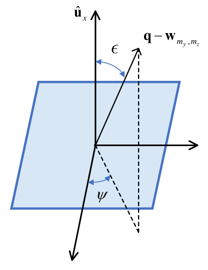
Figure 2: Illustration of the angles for the directional gain pattern for each IRS element.

We assume that the direct link between the BS and the user is negligible. In the preliminary version of this work [1], we mainly pay attention to the variations in signal amplitude across different reflecting elements, and the directional gain pattern of each element is essentially modelled by its projected aperture. In this paper, we consider a generic directional gain pattern for each reflecting element given below [26]

$$G_{e}(\epsilon,\psi)=\begin{cases}\gamma\prime\cos^{2q\prime}(\epsilon),&\epsilon\in\left[\left.0,\frac{\pi}{2}\right)\right.,\psi\in\left[0,2\pi\right]\\ 0,&\text{otherwise}\end{cases},$$ (3)

where $\epsilon$ and $\psi$ are the elevation and azimuth angles as shown in Fig. 2, $q\prime$ determines the directivity of the element, and $\gamma\prime$ is the maximum gain in the boresight direction ($\epsilon=0$), whose value depends on $q\prime$. According to the law of power conservation, we have [26]

$$\varoiint_{S}G_{e}(\epsilon,\psi)\mathrm{d}\Omega=\int_{0}^{2\pi}\mathrm{d}\psi\int_{0}^{\frac{\pi}{2}}\gamma\prime\cos^{2q\prime}(\epsilon)\sin(\epsilon)\mathrm{d}\epsilon=4\pi,$$ (4)

where $S$ is the surface of a semisphere and $\Omega$ is the solid angle. Therefore, the modelling parameters $\gamma\prime$ and $q\prime$ in (3) should follow the relationship [26]

$$\gamma\prime=2(2q\prime+1).$$ (5)

Furthermore, since the effective aperture of any antenna element is proportional to its gain[26], the maximum effective aperture $\mu$ of such a reflecting element is

$$\mu\triangleq\frac{\lambda^{2}}{4\pi}\gamma\prime=\frac{\lambda^{2}}{2\pi}(2q\prime+1).$$ (6)

Based on the Friis Transmission Equation, the ratio of the intercepted power by each IRS element and that transmitted by a source can be expressed as [38, 26]

$$P_{r}/P_{t}=\left(\frac{\lambda}{4\pi r}\right)^{2}G_{t}G_{e}(\epsilon,\psi),$$ (7)

where $r$ is the link distance between the transmit antenna and a given IRS element, and $G_{t}$ is the gain of the transmit antenna. By assuming $G_{t}=1$, it then follows from (1) and (7) that the channel power gain between the BS and the $\left(m_{y},m_{z}\right)$-th reflecting element can be modelled as

$$a_{m_{y},m_{z}}(r_{q},\theta_{q},\phi_{q})=\left(\frac{\lambda}{4\pi r_{q,m_{y},m_{z}}}\right)^{2}\gamma\prime\cos^{2q\prime}(\epsilon_{q}),$$ (8)

where $\cos(\epsilon_{q})$ is the projection between the signal propagation direction and the normal vector of the element surface, given by

$$\cos(\epsilon_{q})=\frac{\left(\mathbf{q}-\mathbf{w}_{m_{y},m_{z}}\right)^{T}\hat{\mathbf{u}}_{x}}{\left\|\mathbf{q}-\mathbf{w}_{m_{y},m_{z}}\right\|},$$ (9)

with $\hat{\mathbf{u}}_{x}$ denoting a unit vector along the $x$-axis, and regarded as the normal vector of any IRS reflecting element. By substituting (9) into (8), the channel power gain can be further expressed as (10) shown at the top of the next page. Likewise, the channel power gain between the $\left(m_{y},m_{z}\right)$-th IRS element and the user can be expressed as (10) at the top of the next page.

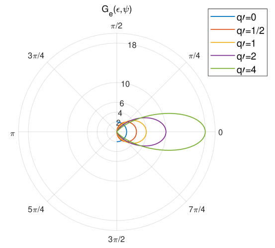
Figure 3: Directional gain pattern of IRS’s reflecting elements for different parameters $q\prime$.

$$a_{m_{y},m_{z}}(r_{q},\theta_{q},\phi_{q})=\left(\frac{\lambda}{4\pi r_{q}}\right)^{2}\frac{\gamma\prime\Psi_{q}^{2q\prime}}{\left[1-2m_{y}\varepsilon_{q}\Phi_{q}-2m_{z}\varepsilon_{q}\Theta_{q}+(m_{y}^{2}+m_{z}^{2})\varepsilon_{q}^{2}\right]^{q\prime+1}}.$$ (10)

$$b_{m_{y},m_{z}}(r_{p},\theta_{p},\phi_{p})=\left(\frac{\lambda}{4\pi r_{p}}\right)^{2}\frac{\gamma\prime\Psi_{p}^{2q\prime}}{\left[1-2m_{y}\varepsilon_{p}\Phi_{p}-2m_{z}\varepsilon_{p}\Theta_{p}+(m_{y}^{2}+m_{z}^{2})\varepsilon_{p}^{2}\right]^{q\prime+1}}.$$ (10)

The channel vector between BS and the XL-IRS is denoted as $\mathbf{h}\in\mathbb{C}^{M\times 1}$, whose entries are given by

$$h_{m_{y},m_{z}}=\sqrt{a_{m_{y},m_{z}}\left(r_{q},\theta_{q},\phi_{q}\right)}e^{-j\frac{2\pi}{\lambda}r_{q,m_{y},m_{z}}},\forall m_{y},m_{z}.$$ (10)

Similarly, the channel vector between the XL-IRS and the user is denoted as $\mathbf{g}\in\mathbb{C}^{M\times 1}$, whose entries are given by

$$g_{m_{y},m_{z}}=\sqrt{b_{m_{y},m_{z}}\left(r_{p},\theta_{p},\phi_{p}\right)}e^{-j\frac{2\pi}{\lambda}r_{p,m_{y},m_{z}}},\forall m_{y},m_{z}.$$ (11)

Further denote the phase shift introduced by the $(m_{y},m_{z})$-th IRS element as $\theta_{m_{y},m_{z}}$, and $\mathbf{\Theta}\in\mathbb{C}^{M\times M}$ is a diagonal matrix, with the diagonal entries given by $e^{j\theta_{m_{y},m_{z}}}$. Then the received signal at the user can be obtained as

$$y=\mathbf{g}^{T}\mathbf{\Theta}\mathbf{h}\sqrt{P}s+n,$$ (12)

where $P$ and $s$ denote the transmit power and information-bearing symbol, respectively; $n\sim\mathcal{CN}(0,\sigma^{2})$ is the additive white Gaussian noise (AWGN) at the user.

Thus, the SNR at the user can be formulated as

$$\gamma=\bar{P}\left|\mathbf{g}^{T}\mathbf{\Theta}\mathbf{h}\right|^{2},$$ (13)

where $\bar{P}\triangleq\frac{P}{\sigma^{2}}$.

III Performance Analysis

In this section, we mainly focus on the performance analysis including the SNR’s lower- and upper-bounds and its asymptotic analysis as $M$ goes to infinity, based on the generic XL-IRS-aided system model and the SNR expression in (13).

III-A SNR Lower- and Upper-Bounds

From (13), the optimal phase shifting by the XL-IRS can be given by

$$\theta_{m_{y},m_{z}}=\frac{2\pi}{\lambda}r_{q,m_{y},m_{z}}+\frac{2\pi}{\lambda}r_{p,m_{y},m_{z}}.$$ (14)

Therefore, the maximum SNR at the user can be expressed as

$$\gamma=\bar{P}\left(\sum_{m_{y}}\sum_{m_{z}}\left|h_{m_{y},m_{z}}\right|\left|g_{m_{y},m_{z}}\right|\right)^{2}.$$ (15)

By substituting (10), (10), (10) and (11) into (15), we can obtain the resulting SNR as (16), shown at the top of the page. Furthermore, motivated by the similar methods in [10], the double summation in (16) can be approximately transformed into its corresponding double integral based on the fact that $\varepsilon_{q}\ll 1$ and $\varepsilon_{p}\ll 1$. Thus, by following the above approximation, the received SNR can be rewritten in an integral form as (16), shown at the top of the page.

$$\gamma=\left(\frac{\lambda}{4\pi}\right)^{4} \frac{\gamma\prime^{2}\bar{P}\Psi_{q}^{2q\prime}\Psi_{p}^{2q\prime}}{r_{q}^{2}r_{p}^{2}}\left|\sum_{m_{y}}\sum_{m_{z}}\frac{1}{\left[1-2m_{y}\varepsilon_{q}\Phi_{q}-2m_{z}\varepsilon_{q}\Theta_{q}+(m_{y}^{2}+m_{z}^{2})\varepsilon_{q}^{2}\right]^{(q\prime+1)/2}}\right.$$ (16)

$$\left.\times\frac{1}{\left[1-2m_{y}\varepsilon_{p}\Phi_{p}-2m_{z}\varepsilon_{p}\Theta_{p}+(m_{y}^{2}+m_{z}^{2})\varepsilon_{p}^{2}\right]^{(q\prime+1)/2}}\right|^{2}.$$

$$\gamma\simeq\left(\frac{\lambda}{4\pi}\right)^{4}\frac{\gamma\prime^{2}\bar{P}\Psi_{q}^{2q\prime}\Psi_{p}^{2q\prime}}{d^{4}r_{q}^{2}r_{p}^{2}}$$ (16)

$$\times\left|\int_{-\frac{L_{z}}{2}}^{\frac{L_{z}}{2}}\int_{-\frac{L_{y}}{2}}^{\frac{L_{y}}{2}}\frac{\mathrm{d}y\mathrm{d}z}{\left[1-\frac{2}{r_{q}}y\Phi_{q}-\frac{2}{r_{q}}z\Theta_{q}+\frac{1}{r_{q}^{2}}(y^{2}+z^{2})\right]^{(q\prime+1)/2}\left[1-\frac{2}{r_{p}}y\Phi_{p}-\frac{2}{r_{p}}z\Theta_{p}+\frac{1}{r_{p}^{2}}(y^{2}+z^{2})\right]^{(q\prime+1)/2}}\right|^{2}.$$

Note that obtaining a closed-form expression for the double integral in (16) is challenging in general. In the following, we will first discuss some special cases for $q\prime$ in (3).

• (1) Semi-isotropic pattern: $q\prime=0$ and $\gamma\prime=2$, so that

  $$G_{e}(\epsilon,\psi)=\begin{cases}2,&\epsilon\in\left[\left.0,\frac{\pi}{2}\right)\right.,\psi\in\left[0,2\pi\right]\\ 0,&\text{otherwise}\end{cases}$$ (16)

• (2) Cosine pattern (based on projected aperture): $q\prime=\frac{1}{2}$ and $\gamma\prime=4$, so that

  $$G_{e}(\epsilon,\psi)=\begin{cases}4\cos(\epsilon),&\epsilon\in\left[\left.0,\frac{\pi}{2}\right)\right.,\psi\in\left[0,2\pi\right]\\ 0,&\text{otherwise}\end{cases}$$ (17)

• (3) Cosine-square pattern: $q\prime=1$ and $\gamma\prime=6$, so that

  $$G_{e}(\epsilon,\psi)=\begin{cases}6\cos^{2}(\epsilon),&\epsilon\in\left[\left.0,\frac{\pi}{2}\right)\right.,\psi\in\left[0,2\pi\right]\\ 0,&\text{otherwise}\end{cases}$$ (18)

Fig. 3 plots different directional gain patterns of IRS’s reflecting elements in (3) versus the angle $\epsilon$. It can be observed that power will be radiated into just one half of the space, i.e., $0\leq\epsilon\leq\pi/2$. Besides, for a larger directivity parameter $q\prime$, there exists a stronger beam with respect to the element’s boresight direction ($\epsilon=0$).

Theorem 1

For XL-IRS-aided communication, the resulting SNR in (16) is bounded by

$$f(R_{1},q\prime)\leq\gamma\leq f(R_{2},q\prime),$$ (19)

where the function $f(R,q\prime)$ is defined as (20) shown at the top of the page;

$$f(R,q\prime)\triangleq\left(\frac{\lambda}{4\pi}\right)^{4}\frac{\gamma\prime^{2}\bar{P}\Psi_{q}^{2q\prime}\Psi_{p}^{2q\prime}}{d^{4}r_{q}^{2}r_{p}^{2}}$$ (20)

$$\times\left|\int_{0}^{2\pi}\mathrm{d}\zeta\int_{0}^{R}\frac{r\mathrm{d}r}{\left[1-\frac{2r}{r_{q}}\Phi_{q}\cos\zeta-\frac{2r}{r_{q}}\Theta_{q}\sin\zeta+\frac{r^{2}}{r_{q}^{2}}\right]^{(q\prime+1)/2}\left[1-\frac{2r}{r_{p}}\Phi_{p}\cos\zeta-\frac{2r}{r_{p}}\Theta_{p}\sin\zeta+\frac{r^{2}}{r_{p}^{2}}\right]^{(q\prime+1)/2}}\right|^{2}.$$

$R_{1}$ and $R_{2}$ denote the radii of the inscribed disk and circumscribed disk of the rectangular region $L_{y}\times L_{z}$ occupied by the XL-IRS as shown in Fig. 4, given by

$$R_{1}=\frac{1}{2}\min\left\{L_{y},L_{z}\right\},$$ (20)

$$R_{2}=\frac{1}{2}\sqrt{L_{y}^{2}+L_{z}^{2}}.$$

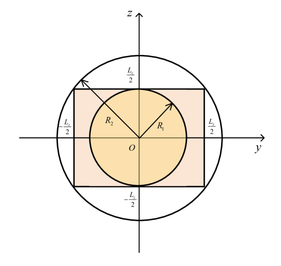
Figure 4: The inscribed and circumscribed disks of the rectangular region $L_{y}\times L_{z}$ occupied by the XL-IRS.

Proof:

Note that the resulting SNR is expressed as a double integral form over the region $L_{y}\times L_{z}$, based on the Cartesian coordinate system, and the integrand is meanwhile positive. Theorem 1 can be verified by scaling this rectangular integral region with its inscribed disk and circumscribed disk that have radii $R_{1}$ and $R_{2}$, respectively. It then follows from the variable transformations that lower- and upper-bounds of the SNR in (19) can be obtained as an integral in polar coordinate. ∎

For convenience, we define a distance ratio as $\rho\triangleq r_{q}/r_{p}$, which represents the ratio of the distance from the BS to the center of the XL-IRS over that from the user to the XL-IRS center. Without loss of generality, it can be assumed that $0<\rho\leq 1$ due to symmetry.

Lemma 1

If the BS and the user are both located along the boresight of the XL-IRS, i.e., near the $x$-axis with $\Phi_{q},\Phi_{p}\ll\frac{r_{q}}{L_{y}}$ and $\Theta_{q},\Theta_{p}\ll\frac{r_{q}}{L_{z}}$, we have

$$\frac{\mu^{2}\bar{P}}{4d^{4}}G(R_{1},q\prime)\leq\gamma\leq\frac{\mu^{2}\bar{P}}{4d^{4}}G(R_{2},q\prime),$$ (21)

where $\mu$ is the maximum effective aperture of each reflecting element defined in (6), and the function $G(R,q\prime)$ is defined as

$$G(R,q\prime)\triangleq\left[\rho\int_{0}^{\arctan\frac{R}{r_{q}}}\frac{\cos^{2q\prime}\alpha\tan\alpha\mathrm{d}\alpha}{\left[\rho^{2}+(1-\rho^{2})\cos^{2}\alpha\right]^{(q\prime+1)/2}}\right]^{2}.$$ (22)

Proof:

Please refer to Appendix A. ∎

Lemma 2

For the special case with the cosine gain pattern based on the projected aperture in (17), i.e., $q\prime=\frac{1}{2}$, under the same condition as Lemma 1, lower- and upper-bounds of the SNR can be further expressed as

$$\begin{cases}\frac{\mu^{2}\bar{P}}{4d^{4}}G\left(R_{1},\frac{1}{2}\right)\leq\gamma\leq\frac{\mu^{2}\bar{P}}{4d^{4}}G\left(R_{2},\frac{1}{2}\right),&0<\rho<1\\ \\ \gamma=\frac{\mu^{2}\bar{P}}{\pi^{2}d^{4}}\arctan^{2}\frac{\left(\frac{L_{y}}{2r_{q}}\right)\left(\frac{L_{z}}{2r_{q}}\right)}{\sqrt{\left(\frac{L_{y}}{2r_{q}}\right)^{2}+\left(\frac{L_{z}}{2r_{q}}\right)^{2}+1}},&\rho=1\end{cases},$$ (23)

where the function $G\left(R,\frac{1}{2}\right)$ with $0<\rho<1$ can be obtained in closed-form as

$$G \left(R,\frac{1}{2}\right)\triangleq\frac{4\rho}{1-\rho^{2}}\Bigg{[}F\left(\frac{1}{2}\arctan\frac{\sqrt{1-\rho^{2}}}{\rho}\bigg{|}2\right)$$ (24)

$$\qquad-F\left(\frac{1}{2}\arctan\left(\frac{\sqrt{1-\rho^{2}}}{\rho}\cos\left(\arctan\frac{R}{r_{q}}\right)\right)\bigg{|}2\right)\Bigg{]}^{2},$$

and $F(\vartheta|k)=\int_{0}^{\vartheta}\frac{1}{\sqrt{1-k\sin^{2}\beta}}\mathrm{d}\beta$ is the incomplete Elliptic Integral of the First Kind [39].

Proof:

The proof follows the similar steps as Appendix A of [1], which is omitted for brevity. ∎

Lemma 3

For the special case with the cosine-square gain pattern in (18), i.e., $q\prime=1$, under the same condition as Lemma 1, lower- and upper- bounds of the SNR can be further expressed as

$$\frac{\mu^{2}\bar{P}}{4d^{4}}G(R_{1},1)\leq\gamma\leq\frac{\mu^{2}\bar{P}}{4d^{4}}G(R_{2},1),$$ (25)

where the function $G(R,1)$ is given in closed-form as (26), shown at the top of the page.

$$G(R,1)\triangleq\begin{cases}\frac{\rho^{2}}{4\left(1-\rho^{2}\right)^{2}}\Bigg{[}\ln\left[\rho^{2}+(1-\rho^{2})\cos^{2}\left(\arctan\frac{R}{r_{q}}\right)\right]\Bigg{]}^{2},&0<\rho<1\\ \\ \frac{1}{4}\Bigg{[}\cos^{2}\left(\arctan\frac{R}{r_{q}}\right)-1\Bigg{]}^{2},&\rho=1\end{cases}.$$ (26)

Proof:

Please refer to Appendix B. ∎

III-B Asymptotic Analysis

$$\lim_{L_{y},L_{z}\rightarrow\infty}\gamma=\frac{\lambda^{4}\rho^{2}}{16\pi^{2}d^{4}}(2q\prime+1)^{2}\bar{P}\left[\int_{0}^{\pi/2}\frac{\cos^{2q\prime}\alpha\tan\alpha\mathrm{d}\alpha}{\left[\rho^{2}+(1-\rho^{2})\cos^{2}\alpha\right]^{(q\prime+1)/2}}\right]^{2}.$$ (26)

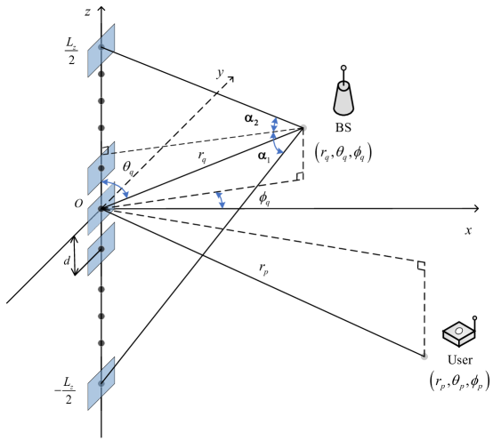
Figure 5: Wireless communication with ULA-based XL-IRS.

Lemma 4

Under the same condition as Lemma 1, the asymptotic SNR as the XL-IRS size goes to infinity can be expressed as (26), shown at the top of the next page.

Proof:

As the IRS size $L_{y},L_{z}\rightarrow\infty$, the radii of the inscribed disk and circumscribed disk of the IRS region $L_{y}\times L_{z}$ defined in (20) also go to infinity, i.e., $R_{1},R_{2}\rightarrow\infty$. It can be proved that the SNR lower- and upper-bounds given by Lemma 1 approach to the same limit due to the identical form of the function $G(R,q\prime)$ with $R\rightarrow\infty$. Therefore, the asymptotic SNR in (26) can be obtained according to the Squeeze Theorem [40]. ∎

It can be shown that the asymptotic SNR is only determined by the directivity parameter $q\prime$ and the distance ratio $\rho$. Furthermore, it is worth mentioning that the convergence of SNR expression depends on the integral in (26).

In particular, for the special case of $\rho=1$, we have

$$\lim_{L_{y},L_{z}\rightarrow\infty}\gamma=\frac{\lambda^{4}}{64\pi^{2}d^{4}}\left(2+\frac{1}{q\prime}\right)^{2}\bar{P}.$$ (26)

To gain more insights, we will also discuss some special cases for $q\prime$ and derive closed-form expressions for the asymptotic SNR. Firstly, the asymptotic SNR under $q\prime=\frac{1}{2}$ in (26) is

$$\lim_{L_{y},L_{z}\rightarrow\infty}\gamma=\begin{cases}\frac{\rho}{1-\rho^{2}}\frac{\lambda^{4}}{\pi^{2}d^{4}}\bar{P}\left[F\left(\frac{1}{2}\arctan\frac{\sqrt{1-\rho^{2}}}{\rho}\bigg{|}2\right)\right]^{2},&0<\rho<1\\ \\ \frac{\lambda^{4}}{4\pi^{2}d^{4}}\bar{P},&\rho=1\end{cases}.$$ (27)

Besides, the asymptotic SNR under $q\prime=1$ in (26) is

$$\lim_{L_{y},L_{z}\rightarrow\infty}\gamma=\begin{cases}\frac{\rho^{2}(\ln\rho)^{2}}{(1-\rho^{2})^{2}}\frac{9\lambda^{4}}{4\pi^{2}d^{4}}\bar{P},&0<\rho<1\\ \\ \frac{9\lambda^{4}}{64\pi^{2}d^{4}}\bar{P},&\rho=1\end{cases}.$$ (28)

Note that the asymptotic SNR in (26) will go to infinity by letting $q\prime=0$, which is expected since modelling each reflecting element semi-isotropically would lead to unbounded power when the XL-IRS size goes to infinity. By contrast, the SNR with considering non-isotropic directional gain pattern of IRS’s reflecting elements, e.g., $q\prime=\frac{1}{2}$ or $q\prime=1$, will lead to a constant value in (27) and (28) as the IRS size increases, which only depends on the distance ratio $\rho$. This implies that for XL-IRS-aided communication system, it is necessary to take into account the impact of the directivity of each reflecting element so as to obey the law of power conservation.

III-C Conventional UPW Model

As a comparison, the conventional UPW model that also takes into account the directional gain pattern of IRS’s reflecting elements can be expressed as

$$\gamma_{UPW}=\frac{M^{2}\beta_{0}^{2}\bar{P}}{r_{q}^{2}r_{p}^{2}}G_{e}\left(\theta_{q},\phi_{q}\right)AF\left(\theta_{q},\phi_{q}\right)\times G_{e}\left(\theta_{p},\phi_{p}\right)AF\left(\theta_{p},\phi_{p}\right),$$ (29)

which follows based on the approximation that all reflecting elements share approximately the same AoA/AoD and link distances; $\beta_{0}$ is the channel gain at the reference distance of 1 meter (m), $G_{e}(\theta,\phi)$ accounts for the directional gain pattern, and $AF(\theta,\phi)$ accounts for the array factor[26], expressed as

$$AF(\theta,\phi)=\frac{1}{M}\frac{\sin\left(\frac{M_{y}}{2}kd\Phi\right)}{\sin\left(\frac{1}{2}kd\Phi\right)}\frac{\sin\left(\frac{M_{z}}{2}kd\Theta\right)}{\sin\left(\frac{1}{2}kd\Theta\right)},$$ (30)

where $k=\frac{2\pi}{\lambda}$ is the wave number; $\Phi=\sin\theta\sin\phi$, $\Theta=\cos\theta$.

Note that the first part of the SNR expression (29) is well known as the square power scaling law for IRS-assisted communication [16], where the SNR increases linearly with the square of the number of IRS reflecting elements, i.e., $M^{2}$. It can be observed that such a fundamental result (29) is also related with the AoA/AoD via the directional gain pattern $G_{e}(\theta,\phi)$ and the array factor $AF(\theta,\phi)$. Furthermore, it is worth mentioning that the above result is valid only when both link distances $r_{q}$ and $r_{p}$ are sufficiently large by comparison with the IRS dimension, i.e., $M$ is moderately large. This makes it possible that the far-field propagation model can apply to both the whole IRS as well as its each individual element. However, when $M$ is extremely large, the conventional model may no more hold since the square power scaling law reveals that the SNR would correspondingly increase without any limited bound, which obviously violates the law of power conservation. Conversely, our new result shows that under the practical NUSW model, the SNR increases with $M$, but with a diminishing return, and eventually converge to a constant that depends on the distance ratio $\rho$, as well as the directivity parameter $q\prime$ of each reflecting element.

$$\gamma\simeq\frac{A^{2}\bar{P}\Psi_{q}\Psi_{p}}{16\pi^{2}d^{2}r_{q}^{2}r_{p}^{2}}\left|\int_{-\frac{L_{z}}{2}}^{\frac{L_{z}}{2}}\frac{\mathrm{d}z}{\left[\left(1-\frac{2}{r_{q}}z\cos\theta_{q}+\frac{z^{2}}{r_{q}^{2}}\right)\left(1-\frac{2}{r_{p}}z\cos\theta_{p}+\frac{z^{2}}{r_{p}^{2}}\right)\right]^{(q\prime+1)/2}}\right|^{2}.$$ (31)

III-D ULA-based XL-IRS

To gain more insights, we further consider the special case of ULA-based XL-IRS, i.e., $M_{y}=1$ and $M_{z}=M$. In this case, by substituting $y=0$ and $\mathrm{d}y=d$ into (16), the SNR expression can be reduced to a simpler form as (31), shown at the top of the page.

Lemma 5

For wireless communication assisted by ULA-based XL-IRS, when the link distances satisfy $r_{q}\ll r_{p}$ (i.e., $\rho\rightarrow 0$), the resulting SNR in (31) under the cosine gain pattern based on projected aperture, i.e., $q\prime=\frac{1}{2}$, can be expressed in closed-form as

$$\gamma=\frac{\lambda^{4}\bar{P}\Psi_{p}\cos\phi_{q}}{4\pi^{4}d^{2}r_{p}^{2}}\left[F\left(\frac{\alpha_{1}}{2}\bigg{|}2\right)+F\left(\frac{\alpha_{2}}{2}\bigg{|}2\right)\right]^{2},$$ (31)

where $\alpha_{1}=\arctan\frac{L_{z}/2+r_{q}\cos\theta_{q}}{r_{q}\sin\theta_{q}}$ and $\alpha_{2}=\arctan\frac{L_{z}/2-r_{q}\cos\theta_{q}}{r_{q}\sin\theta_{q}}$.

Proof:

The proof follows the similar steps as Appendix B of [1], which is omitted for brevity. ∎

It is worth mentioning that the additional condition $r_{q}\ll r_{p}$ given by Lemma 5 is consistent with the commonly used IRS deployment strategy [15, 21]. Specifically, it has been demonstrated that IRS should be deployed either close to the BS or to the user for maximizing the received SNR. Lemma 5 shows that with the developed near-field model, the resulting SNR for the special case of ULA-based XL-IRS depends on the IRS size $L_{z}$, the link distance $r_{q}$ and the AoA $\theta_{q}$, and is in general expressed in terms of the two geometric parameters, $\alpha_{1}$ and $\alpha_{2}$, which are the angles formed by the line segments connecting the BS location and its projection to the IRS, as well as the two ends of the IRS, as illustrated in Fig. 5. In particular, $\alpha_{1}+\alpha_{2}$ is termed as the angular span [9]. It is observed that for any AoA $\theta_{q}$, both $\alpha_{1}$ and $\alpha_{2}$ increase with the IRS size $L_{z}$ and decrease with the link distance $r_{q}$ between the BS and the XL-IRS center. Due to the fact that the Elliptic Integral function $F(\vartheta|2)$ monotonically increases with $\vartheta$, the resulting SNR $\gamma$ in (31) increases with $L_{z}$ but decreases with $r_{q}$, as expected. Furthermore, Lemma 5 shows that under the practical NUSW model, the SNR increases with $L_{z}$ with a diminishing return. Note that this result differs from the conventional square power scaling law obtained based on the UPW model, where the SNR increases unboundedly with the IRS size [16, 21]. In particular, it can be shown that as $L_{z}\rightarrow\infty$, we reach the extreme case, i.e., $\alpha_{1}=\alpha_{2}=\frac{\pi}{2}$, leading to the following lemma.

Lemma 6

Under the same condition as Lemma 5, the asymptotic SNR for ULA-based XL-IRS is

$$\lim_{L_{z}\rightarrow\infty}\gamma=\frac{\lambda^{4}\bar{P}\Psi_{p}\cos\phi_{q}}{\pi^{4}d^{2}r_{p}^{2}}\left[F\left(\frac{\pi}{4}\bigg{|}2\right)\right]^{2}=1.7188\times\frac{\lambda^{4}\bar{P}\Psi_{p}}{\pi^{4}d^{2}r_{p}^{2}}\cos\phi_{q}.$$ (32)

IV Extension to Multi-Antenna BS

Our previous analysis assumes that the BS has a single antenna so as to reveal the most important insights. In this section, we consider the MISO setup where the BS is equipped with multiple antennas in the form of UPA architecture. For simplicity, we assume that the UPA at the BS is parallel to the IRS, as illustrated in Fig. 6. The number of antennas at the BS is denoted as $N=N_{y}N_{z}$, where $N_{y}$ and $N_{z}$ denote the number of antennas along the $y$- and $z$-axis, respectively, and the antenna element separation is $d_{0}$. Thus, the central location of the $\left(n_{y},n_{z}\right)$-th antenna is $\mathbf{u}_{n_{y},n_{z}}=\left[r_{q}\Psi_{q},r_{q}\Phi_{q}+n_{y}d_{0},r_{q}\Theta_{q}+n_{z}d_{0}\right]^{T}$, where $n_{y}=0,\pm 1,\cdots,\pm\left(N_{y}-1\right)/2$ and $n_{z}=0,\pm 1,\cdots,\pm\left(N_{z}-1\right)/2$. The distance between the $\left(n_{y},n_{z}\right)$-th antenna at the BS and the $\left(m_{y},m_{z}\right)$-th reflecting element is

$$r_{q,m_{y},m_{z},n_{y},n_{z}}=\left\|\mathbf{u}_{m_{y},m_{z}}-\mathbf{w}_{m_{y},m_{z}}\right\|,$$ (33)

which can be further expressed as (34) at the top of the next page with $\varepsilon_{q_{0}}\triangleq\frac{d_{0}}{r_{q}}\ll 1$ [10, 1].

$$r_{q,m_{y},m_{z},n_{y},n_{z}}$$ (34)

$$\quad=r_{q}\sqrt{1+2\Phi_{q}(n_{y}\varepsilon_{q_{0}}-m_{y}\varepsilon_{q})+2\Theta_{q}(n_{z}\varepsilon_{q_{0}}-m_{z}\varepsilon_{q})+(n_{y}\varepsilon_{q_{0}}-m_{y}\varepsilon_{q})^{2}+(n_{z}\varepsilon_{q_{0}}-m_{z}\varepsilon_{q})^{2}}.$$

Thus, the channel matrix between the BS and XL-IRS is denoted as $\mathbf{H}\in\mathbb{C}^{M\times N}$, whose entries are given by

$$h_{m_{y},m_{z},n_{y},n_{z}}=\sqrt{a_{m_{y},m_{z},n_{y},n_{z}}\left(r_{q},\theta_{q},\phi_{q}\right)}\times e^{-j\frac{2\pi}{\lambda}r_{q,m_{y},m_{z},n_{y},n_{z}}},\forall m_{y},m_{z},n_{y},n_{z},$$ (34)

where the channel power gain $a_{m_{y},m_{z},n_{y},n_{Z}}(r_{q},\theta_{q},\phi_{q})$ between the $(n_{y},n_{z})$-th antenna at the BS and the $(m_{y},m_{z})$-th reflecting element at the IRS is given by (35) at the top of the page.

$$a_{m_{y},m_{z},n_{y},n_{Z}}(r_{q},\theta_{q},\phi_{q})$$ (35)

$$=\left(\frac{\lambda}{4\pi r_{q}}\right)^{2}\frac{\gamma\prime\Psi_{q}^{2q\prime}}{\left[1+2(n_{y}\varepsilon_{q_{0}}-m_{y}\varepsilon_{q})\Phi_{q}+2(n_{z}\varepsilon_{q_{0}}-m_{z}\varepsilon_{q})\Theta_{q}+(n_{y}\varepsilon_{q_{0}}-m_{y}\varepsilon_{q})^{2}+(n_{z}\varepsilon_{q_{0}}-m_{z}\varepsilon_{q})^{2}\right]^{q\prime+1}}.$$

Therefore, the SNR at the user can be expressed as

$$\gamma=\bar{P}\left|\mathbf{g}^{T}\mathbf{\Theta}\mathbf{H}\mathbf{v}\right|^{2},$$ (35)

where $\mathbf{v}\in\mathbb{C}^{N\times 1}$ is a beamforming vector, with $\|\mathbf{v}\|=1$.

Similarly, it is assumed that the IRS is deployed at the vicinity of the user, so that the user is located in the near-field region of the IRS while the BS is in the far- field region. By letting $\varepsilon_{q}\rightarrow 0$ in (35), the channel matrix vector $\mathbf{H}\in\mathbb{C}^{M\times N}$ can be written as a rank-one matrix as

$$\mathbf{H}=\sqrt{\frac{\lambda^{2}\gamma\prime\Psi_{q}^{2q^{\prime}}}{16\pi^{2}r_{q}^{2}}}e^{-j\frac{2\pi}{\lambda}r_{q}}\mathbf{a}_{R}\left(\theta_{q},\phi_{q}\right)\mathbf{a}_{T}^{H}\left(\theta_{q},\phi_{q}\right),$$ (36)

where $\mathbf{a}_{R}\left(\theta_{q},\phi_{q}\right)\in\mathbb{C}^{M\times 1}$ is the receive array response vector at the XL-IRS, given by

$$\mathbf{a}_{R}(\theta_{q},\phi_{q})=\left[e^{j\frac{2\pi}{\lambda}m_{y}d\Phi_{q}}\right]_{1\times M_{y}}^{T}\otimes\left[e^{j\frac{2\pi}{\lambda}m_{z}d\Theta_{q}}\right]_{1\times M_{z}}^{T},$$ (37)

where the symbol $\otimes$ denotes the Kronecker product. Similarly, denote the transmit array response vector at the BS as $\mathbf{a}_{T}\left(\theta_{q},\phi_{q}\right)\in\mathbb{C}^{N\times 1}$, given by

$$\mathbf{a}_{T}(\theta_{q},\phi_{q})=\left[e^{j\frac{2\pi}{\lambda}n_{y}d_{0}\Phi_{q}}\right]_{1\times N_{y}}^{T}\otimes\left[e^{j\frac{2\pi}{\lambda}n_{z}d_{0}\Theta_{q}}\right]_{1\times N_{z}}^{T}.$$ (38)

Based on [21], the optimal transmit beamforming vector at the BS for SNR maximization is

$$\mathbf{v}^{*}=\frac{\mathbf{a}_{T}\left(\theta_{q},\phi_{q}\right)}{\sqrt{N}}.$$ (39)

Furthermore, with the optimal phase shifting by the XL-IRS in (13), the maximum SNR at the user reduces to

$$\gamma=N\bar{P}\left|\sum_{m_{y}}\sum_{m_{z}}\sqrt{\frac{\lambda^{2}\gamma\prime\Psi_{q}^{2q^{\prime}}}{16\pi^{2}r_{q}^{2}}b_{m_{y},m_{z}}\left(r_{p},\theta_{p},\phi_{p}\right)}\right|^{2}.$$ (40)

By substituting (10) into (40), we obatin the summation form of the SNR at the user as (41), shown at the top of the page.

$$\gamma=N\bar{P}\left(\frac{\lambda}{4\pi}\right)^{4}\frac{\gamma\prime^{2}\Psi_{q}^{2q^{\prime}}\Psi_{p}^{2q^{\prime}}}{r_{q}^{2}r_{p}^{2}}\bigg{|}\sum_{m_{y},m_{z}}\frac{1}{\left[1-2m_{y}\varepsilon_{p}\Phi_{p}-2m_{z}\varepsilon_{p}\Theta_{p}+(m_{y}^{2}+m_{z}^{2})\varepsilon_{p}^{2}\right]^{(q^{\prime}+1)/2}}\bigg{|}^{2}.$$ (41)

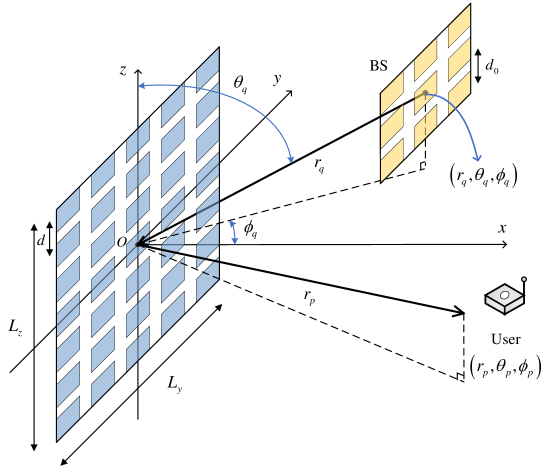
Figure 6: Wireless communication assisted by XL-IRS with multi-antenna BS.

$$\gamma=N\bar{P}\left(\frac{\lambda}{4\pi}\right)^{4}\frac{\gamma\prime^{2}\Psi_{q}^{2q^{\prime}}\Psi_{p}^{2q^{\prime}}}{d^{4}r_{q}^{2}r_{p}^{2}}\bigg{|}\int_{-\frac{L_{z}}{2}}^{\frac{L_{z}}{2}}\int_{-\frac{L_{y}}{2}}^{\frac{L_{y}}{2}}\frac{\mathrm{d}y\mathrm{d}z}{\left[1-\frac{2}{r_{p}}y\Phi_{p}-\frac{2}{r_{p}}z\Theta_{p}+\frac{2}{r_{p}^{2}}(y^{2}+z^{2})\right]^{(q^{\prime}+1)/2}}\bigg{|}^{2}.$$ (41)

Similarly, by approximating the summation with a double integral by using the fact $\varepsilon_{p}\ll 1$, the SNR can be written in an integral form (41) shown at the top of the page. Following the similar derivation in Theorem 1, the SNR is bounded by

$$U(R_{1},q\prime)\leq\gamma\leq U(R_{2},q\prime),$$ (41)

where the function $U(R,q\prime)$ is defined as (42) shown at the top of the page, and the radii $R_{1}$ and $R_{2}$ are also given by (20).

$$U(R,q\prime)\triangleq N\bar{P}\left(\frac{\lambda}{4\pi}\right)^{4}\frac{\gamma\prime^{2}\Psi_{q}^{2q^{\prime}}\Psi_{p}^{2q^{\prime}}}{d^{4}r_{q}^{2}r_{p}^{2}}\bigg{|}\int_{0}^{2\pi}\mathrm{d}\zeta\int_{0}^{R}\frac{r\mathrm{d}r}{\left[1-\frac{2r}{r_{p}}\Phi_{p}\cos\zeta-\frac{2r}{r_{p}}\Theta_{p}\sin\zeta+\frac{r^{2}}{r_{p}^{2}}\right]^{(q^{\prime}+1)/2}}\bigg{|}^{2}.$$ (42)

Lemma 7

If the user is located along the boresight of the XL-IRS, i.e., near the $x$-axis with $\Phi_{p}\ll\frac{r_{p}}{L_{y}}$, $\Theta_{p}\ll\frac{r_{p}}{L_{z}}$, and $q^{\prime}=\frac{1}{2}$, we have

$$U\left(R,\frac{1}{2}\right)\triangleq N\bar{P}\frac{\lambda^{4}\gamma\prime^{2}\Psi_{q}r_{p}^{2}}{16\pi^{2}d^{4}r_{q}^{2}}\bigg{(}\sqrt[4]{\frac{R^{2}}{r_{p}^{2}}+1}-1\bigg{)}^{2}.$$ (42)

Proof:

Please refer to Appendix C. ∎

V Numerical Results

In this section, numerical results are provided to validate our near-field model and theoretical analysis for XL-IRS-aided communications, and also compare our developed model with the conventional UPW model. Unless otherwise stated, the signal wavelength is set as $\lambda=0.125\,$m, and the separation of adjacent IRS elements is $d=\frac{\lambda}{3}$.

V-A SNR Bounds and Asymptotic Analysis

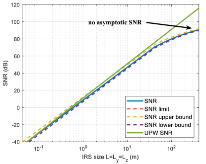
(a) $q\prime=0$

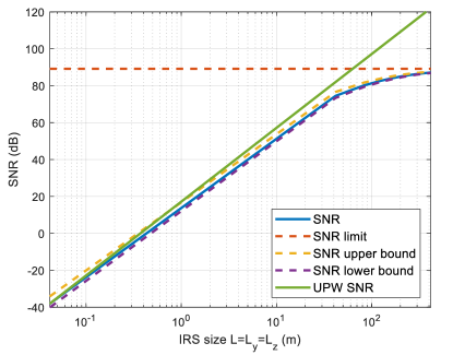
(b) $q\prime=\frac{1}{2}$

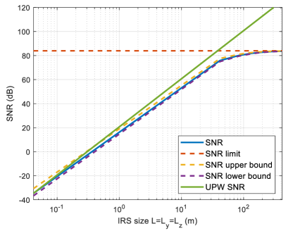
(c) $q\prime=1$

Figure 7: SNR versus IRS size.

Firstly, we present the numerical results of the SNR bounds and its asymptotic performance. Fig. 7 plots the SNR versus the IRS size for a square UPA-based XL-IRS, i.e., $L=L_{y}=L_{z}$. Three directional gain patterns of IRS’s reflecting element based on (16)-(18) for ease of exposition are considered. Additionally, the derived results in the previous sections are compared in Fig. 7, based on the summation in (16), lower- and upper-bounds in (22)-(25), the asymptotic value in (26), (27) and (28), and the conventional UPW model in (29). The transmit SNR is $\bar{P}=90\,\mathrm{dB}$, and the BS and user are assumed to be located at $\mathbf{q}=[10,0,0]^{T}\,\mathrm{m}$ and $\mathbf{p}=[100,0,0]^{T}\,\mathrm{m}$, respectively. It is firstly observed that for UPA-based XL-IRS, the derived bounds in Lemma 1 are sufficiently tight for the SNR estimation. In particular, Figs. 7LABEL:sub@snr_numerical_results_IRS_size_q_1/2 and 7LABEL:sub@snr_numerical_results_IRS_size_q_1 validate our closed-form bounds in (23) and (25). Furthermore, as the IRS size $L$ becomes large, the SNR in Fig. 7LABEL:sub@snr_numerical_results_IRS_size_q_0 goes to infinity eventually, while approaching to a constant in Fig. 7LABEL:sub@snr_numerical_results_IRS_size_q_1/2 and 7LABEL:sub@snr_numerical_results_IRS_size_q_1. This validates our theoretical results in Lemma 4. Besides, it is observed that the conventional UPW model in (29) is approximately consistent with our developed near-field model when the IRS size is not very large. However, as the IRS size exceeds a certain threshold, such two models exhibit drastically different scaling laws, i.e., converging to a constant value versus increasing unboundedly. In summary, the conventional UPW model is valid for most practical cases in terms of the received power, but the accurate near-field modelling needs to be considered when the IRS size becomes significantly large, especially for the asymptotic analysis, which is consistent with the conclusions in [31].

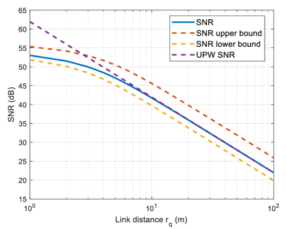
(a) $q\prime=0$

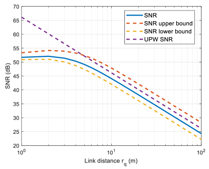
(b) $q\prime=\frac{1}{2}$

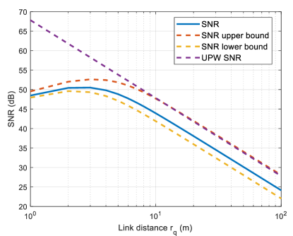
(c) $q\prime=1$

Figure 8: SNR versus link distance $r_{q}$.

Fig. 8 plots the SNR versus the link distance $r_{q}$ between the BS and the IRS center, where the square IRS size is set as $L_{y}=L_{z}\simeq 8\,\mathrm{m}$. We compare the resulting SNR with the following expressions, i.e., the summation form in (16), generic lower- and upper-bounds in (19), and the square power scaling law under the conventional UPW model in (29). The BS direction is set as $(\theta_{q},\phi_{q})=\left(\frac{\pi}{3},\frac{\pi}{6}\right)$, and the user is located at $(r_{p},\theta_{p},\phi_{p})=\left(200\,\mathrm{m},\frac{3\pi}{4},-\frac{\pi}{5}\right)$. It is observed that the SNR bounds given in Theorem 1 are rather accurate, and the conventional UPW model in general over-estimates the SNR values when taking into account the directional gain patterns of IRS’s reflecting elements, as illustrated in Fig. 8LABEL:sub@snr_numerical_results_link_distance_q_1/2 and 8LABEL:sub@snr_numerical_results_link_distance_q_1. In particular, Fig. 8LABEL:sub@snr_numerical_results_link_distance_q_1 reveals that the SNR does not necessarily monotonically decrease with the distance from the BS to the XL-IRS, because it also depends on the gain pattern of each element. Although the BS is deployed close to the IRS, the smaller AoA from the BS to each reflecting element will result in the moderately worse performance when its directional gain pattern is strong in the boresight direction. Therefore, as the link distance $r_{q}$ grows, there might be first a slight rise for the SNR due to the increase of the AoA from the BS to each IRS element.

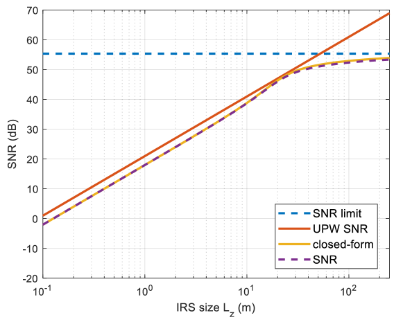
Figure 9: SNR versus IRS size for ULA-based XL-IRS.

V-B ULA-based XL-IRS

Next, for the special case of ULA-based XL-IRS, Fig. 9 plots the SNR versus the IRS size $L_{z}$ based on the summation in (16), derived closed-form expression in (31), the asymptotic limit in (32), and the conventional UPW model in (29). The transmit SNR is $\bar{P}=120\,\mathrm{dB}$, and the BS and user are located at $(r_{q},\theta_{q},\phi_{q})=\left(10\,\mathrm{m},\frac{\pi}{3},\frac{\pi}{6}\right)$ and $(r_{p},\theta_{p},\phi_{p})=\left(100\,\mathrm{m},\frac{3\pi}{4},-\frac{\pi}{5}\right)$, respectively. It is firstly observed that both the closed-form expression (31) and the asymptotic limit (32) match quite well with the actual values. Furthermore, similar to Fig. 7, the UPW expression can accurately predict the SNR values for the moderate-scale IRS. Likewise, as $L_{z}$ goes extremely large, although the SNR under the conventional UPW model increases unboundedly, that under our developed near-field model approaches to a constant value specified in (32). This again demonstrates the importance of proper near-field modelling for communications assisted by XL-IRS.

V-C Multi-Antenna BS

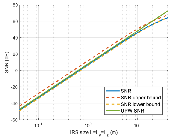
Figure 10: SNR versus IRS size with Multi-Antenna BS.

Lastly, we consider the MISO case where the BS is equipped with a UPA. Fig. 10 plots the SNR versus the IRS size, based on the summation in (40) and closed-form bounds of the SNR in (41). The directional gain pattern of IRS’s reflecting elements is based on (17). The transmit SNR is $\bar{P}=90\,\mathrm{dB}$, and the center of the BS and user are located at $(r_{q},\theta_{q},\phi_{q})=\left(10^{3}\,\mathrm{m},\frac{\pi}{3},-\frac{\pi}{4}\right)$ and $(r_{p},\theta_{p},\phi_{p})=\left(10\,\mathrm{m},\frac{\pi}{2},0\right)$, respectively. It is observed that the derived closed-form bounds can tightly estimate the SNR value when the IRS size is not very large. Furthermore, there exists a notable gap between the conventional UPW model and the accurate near-field model as the IRS size goes large.

VI Conclusions

This paper studied the near-field modelling and performance analysis for wireless communication with XL-IRS. A generic near-field modelling for XL-IRS was developed, by taking into account the directional gain pattern of IRS’s reflecting elements and the variations in received signal amplitude across different reflecting elements. We firstly derived tight lower- and upper-bounds of the received SNR for the UPA-based XL-IRS. To gain more insights, the special case of ULA-based XL-IRS was further considered, together with the extension of our developed near-field modelling to the MISO setup. Numerical results verified our theoretical analysis and demonstrated the necessity of proper near-field modelling for wireless communications aided by XL-IRS.

Appendix A Proof of Lemma 1

When $\Phi_{q},\Phi_{p}\ll\frac{r_{q}}{L_{y}}$ and $\Theta_{q},\Theta_{p}\ll\frac{r_{q}}{L_{z}}$, the double integral in (20) reduces to the following form

$$I= \int_{0}^{2\pi}\mathrm{d}\zeta\int_{0}^{R}\frac{r\mathrm{d}r}{\left[\left(1+\frac{r^{2}}{r_{q}^{2}}\right)\left(1+\frac{r^{2}}{r_{p}^{2}}\right)\right]^{\left(q\prime+1\right)/2}}$$ (43)

$$=2\pi r_{q}^{2}\int_{0}^{\frac{R}{r_{q}}}\frac{r\mathrm{d}r}{\left[\left(r^{2}+1\right)\left(\rho^{2}r^{2}+1\right)\right]^{\left(q\prime+1\right)/2}}.$$

By letting $r=\tan\alpha$, we can transform (43) into

$$I=2\pi r_{q}^{2}\int_{0}^{\arctan\frac{R}{r_{q}}}\frac{\cos^{2q\prime}\alpha\tan\alpha\mathrm{d}\alpha}{[\rho^{2}+(1-\rho^{2})\cos^{2}\alpha]^{(q\prime+1)/2}}.$$ (44)

With Theorem 1, and by substituting (44) into (20), we can have

$$f\left(R,q\prime\right) =\left(\frac{\lambda}{4\pi}\right)^{4}\frac{\gamma\prime^{2}\bar{P}}{d^{4}r_{q}^{2}r_{p}^{2}}I^{2}$$ (45)

$$=\frac{\mu^{2}\bar{P}}{4d^{4}}\left[\rho\int_{0}^{\arctan\frac{R}{r_{q}}}\frac{\cos^{2q\prime}\alpha\tan\alpha\mathrm{d}\alpha}{\left[\rho^{2}+(1-\rho^{2})\cos^{2}\alpha\right]^{(q\prime+1)/2}}\right]^{2}$$

$$=\frac{\mu^{2}\bar{P}}{4d^{4}}G(R,q\prime),$$

where the facts $\gamma\prime=\frac{4\pi}{\lambda^{2}}\mu$ and $\rho=r_{q}/r_{p}$ are used, and then Lemma 1 can be obtained.

Appendix B Proof of Lemma 3

By letting $q\prime=1$, (22) can be expressed as

$$G(R,1) =\left[\rho\int_{0}^{\arctan R/r_{q}}\frac{\cos^{2}\alpha\tan\alpha\mathrm{d}\alpha}{\rho^{2}+(1-\rho^{2})\cos^{2}\alpha}\right]^{2}$$ (46)

$$=\left[\rho\int_{0}^{\arctan R/r_{q}}\frac{\cos\alpha\mathrm{d}(\cos\alpha)}{\rho^{2}+(1-\rho^{2})\cos^{2}\alpha}\right]^{2}.$$

First, for $\rho=1$, (46) can be simplified as

$$G(R,1)=\left[\int_{0}^{\arctan R/r_{q}}\cos\alpha\mathrm{d}(\cos\alpha)\right]^{2}=\frac{1}{4}\Bigg{[}\cos^{2}\left(\arctan\frac{R}{r_{q}}\right)-1\Bigg{]}^{2}.$$ (47)

Next, for $0<\rho<1$, (46) can be further expressed as

$$G(R,1) =\left[\frac{\rho}{1-\rho^{2}}\int_{0}^{\arctan R/r_{q}}\frac{(1-\rho^{2})\cos\alpha\mathrm{d}(\cos\alpha)}{\rho^{2}+(1-\rho^{2})\cos^{2}\alpha}\right]^{2}$$ (48)

$$=\frac{\rho^{2}}{4\left(1-\rho^{2}\right)^{2}}\Bigg{[}\ln\left[\rho^{2}+(1-\rho^{2})\cos^{2}\left(\arctan\frac{R}{r_{q}}\right)\right]\Bigg{]}^{2}.$$

Then, the proof of Lemma 3 is completed.

Appendix C Proof of Lemma 7

With $\Phi_{p}\ll\frac{r_{p}}{L_{y}}$, $\Theta_{p}\ll\frac{r_{p}}{L_{z}}$ and $q\prime=\frac{1}{2}$, the double integral in (42) can reduce to

$$I\prime =\int_{o}^{2\pi}\mathrm{d}\zeta\int_{0}^{R}\frac{r\mathrm{d}r}{\left(1+\frac{r^{2}}{r_{p}^{2}}\right)^{3/4}}=2\pi\left[\left(1+\frac{r^{2}}{r_{p}^{2}}\right)^{1/4}\right]_{0}^{R}$$ (49)

$$=2\pi\left(\sqrt[4]{\frac{R^{2}}{r_{p}^{2}}+1}-1\right).$$

By substituting (49) into (42), we obtain

$$U\left(R,\frac{1}{2}\right)=N\left(\frac{\lambda}{4\pi}\right)^{4}\frac{\gamma\prime^{2}\Psi_{q}\bar{P}}{d^{4}r_{q}^{2}r_{p}^{2}}I\prime^{2}=N\bar{P}\frac{\lambda^{4}\gamma\prime^{2}\Psi_{q}r_{p}^{2}}{16\pi^{2}d^{4}r_{q}^{2}}\bigg{(}\sqrt[4]{\frac{R^{2}}{r_{p}^{2}}+1}-1\bigg{)}^{2}.$$ (50)

Thus, the proof of Lemma 7 is completed.

References

- [1] C. Feng, H. Lu, Y. Zeng, S. Jin, and R. Zhang, “Wireless communication with extremely large-scale intelligent reflecting surface,” in Proc. IEEE/CIC Int. Conf. Commun. China (ICCC Workshops), 2021.
- [2] M. Latva-aho, K. Leppänen, F. Clazzer, and A. Munari, “Key drivers and research challenges for 6G ubiquitous wireless intelligence,” 6G Res. Vis. 1, 6G Flagship, Sep. 2019.
- [3] X. You et al., “Towards 6G wireless communication networks: Vision, enabling technologies, and new paradigm shifts,” Sci. China Inf. Sci., vol. 64, no. 1, pp. 1–74, Nov. 2020.
- [4] W. Saad, M. Bennis, and M. Chen, “A vision of 6G wireless systems: Applications, trends, technologies, and open research problems,” IEEE Netw., vol. 34, no. 3, pp. 134–142, Oct. 2019.
- [5] Y. Zeng and X. Xu, “Toward environment-aware 6G communications via channel knowledge map,” IEEE Wireless Commun., vol. 28, no. 3, pp. 84–91, Mar. 2021.
- [6] E. Björnson, L. Sanguinetti, H. Wymeersch, J. Hoydis, and T. L. Marzetta, “Massive MIMO is a reality—what is next?: Five promising research directions for antenna arrays,” Digit. Signal Process., vol. 94, pp. 3–20, Nov. 2019.
- [7] E. De Carvalho, A. Ali, A. Amiri, M. Angjelichinoski, and R. W. Heath, “Non-stationarities in extra-large-scale massive MIMO,” IEEE Wireless Commun., vol. 27, no. 4, pp. 74–80, Aug. 2020.
- [8] Y. Han, S. Jin, C.-K. Wen, and X. Ma, “Channel estimation for extremely large-scale massive MIMO systems,” IEEE Wireless Commun. Lett., vol. 9, no. 5, pp. 633–637, Jan. 2020.
- [9] H. Lu and Y. Zeng, “How does performance scale with antenna number for extremely large-scale MIMO?” in Proc. IEEE Int. Conf. (ICC), 2021.
- [10] ——, “Communicating with extremely large-scale array/surface: Unified modelling and performance analysis,” IEEE Trans. Wireless Commun., vol. 21, no. 6, pp. 4039–4053, Jun. 2021.
- [11] S. Hu, F. Rusek, and O. Edfors, “Beyond massive MIMO: The potential of data transmission with large intelligent surfaces,” IEEE Trans. Signal Process., vol. 66, no. 10, pp. 2746–2758, May. 2018.
- [12] M. Cui and L. Dai, “Channel estimation for extremely large-scale MIMO: Far-field or near-field?” IEEE Trans. Commun., vol. 70, no. 4, pp. 2663–2677, Jan. 2022.
- [13] T. S. Rappaport, S. Sun, R. Mayzus, H. Zhao, Y. Azar, K. Wang, G. N. Wong, J. K. Schulz, M. Samimi, and F. Gutierrez, “Millimeter wave mobile communications for 5G cellular: It will work!” IEEE Access., vol. 1, pp. 335–349, May. 2013.
- [14] H. Elayan, O. Amin, R. M. Shubair, and M.-S. Alouini, “Terahertz communication: The opportunities of wireless technology beyond 5G,” in Proc. IEEE Int. Conf. Adv. Commun. Technol. Netw.(CommNet), Apr. 2018, pp. 1–5.
- [15] Q. Wu, S. Zhang, B. Zheng, C. You, and R. Zhang, “Intelligent reflecting surface aided wireless communications: A tutorial,” IEEE Trans. Commun., vol. 69, no. 5, pp. 3313–3351, May 2021.
- [16] Q. Wu and R. Zhang, “Intelligent reflecting surface enhanced wireless network via joint active and passive beamforming,” IEEE Trans. Wireless Commun., vol. 18, no. 11, pp. 5394–5409, Nov. 2019.
- [17] C. Huang, A. Zappone, G. C. Alexandropoulos, M. Debbah, and C. Yuen, “Reconfigurable intelligent surfaces for energy efficiency in wireless communication,” IEEE Trans. Wireless Commun., vol. 18, no. 8, pp. 4157–4170, Aug. 2019.
- [18] Q. Wu and R. Zhang, “Towards smart and reconfigurable environment: Intelligent reflecting surface aided wireless network,” IEEE Commun. Mag., vol. 58, no. 1, pp. 106–112, Jan. 2020.
- [19] W. Tang et al., “Wireless communications with reconfigurable intelligent surface: Path loss modeling and experimental measurement,” IEEE Trans. Wireless Commun., vol. 20, no. 1, pp. 421–439, Jan. 2021.
- [20] M. Di Renzo et al., “Smart radio environments empowered by reconfigurable intelligent surfaces: How it works, state of research, and the road ahead,” IEEE J. Sel. Areas Commun., vol. 38, no. 11, pp. 2450–2525, Nov. 2020.
- [21] H. Lu, Y. Zeng, S. Jin, and R. Zhang, “Aerial intelligent reflecting surface: Joint placement and passive beamforming design with 3D beam flattening,” IEEE Trans. Wireless Commun., vol. 20, no. 7, pp. 4128–4143, Feb. 2021.
- [22] E. Björnson and L. Sanguinetti, “Demystifying the power scaling law of intelligent reflecting surfaces and metasurfaces,” in Proc. IEEE Int. Workshop Comput. Adv. Multi Sensor Adapt. Process., Dec. 2019, pp. 549–553.
- [23] K. T. Selvan and R. Janaswamy, “Fraunhofer and fresnel distances: Unified derivation for aperture antennas.” IEEE Antennas Propag. Mag., vol. 59, no. 4, pp. 12–15, Aug. 2017.
- [24] J. Yang, Y. Zeng, S. Jin, C.-K. Wen, and P. Xu, “Communication and localization with extremely large lens antenna array,” IEEE Trans. Wireless Commun., vol. 20, no. 5, pp. 3031–3048, May. 2021.
- [25] C. A. Balanis, Advanced engineering electromagnetics. John Wiley & Sons, 2012.
- [26] ——, Antenna theory: Analysis and Design. John wiley & sons, 2015.
- [27] Z. Zhou, X. Gao, J. Fang, and Z. Chen, “Spherical wave channel and analysis for large linear array in los conditions,” in Proc. IEEE Globecom Workshops (GC Wkshps), Dec. 2015, pp. 1–6.
- [28] B. Friedlander, “Localization of signals in the near-field of an antenna array,” IEEE Trans. Signal Process., vol. 67, no. 15, pp. 3885–3893, Aug. 2019.
- [29] H. Lu and Y. Zeng, “Near-field modeling and performance analysis for multi-user extremely large-scale MIMO communication,” IEEE Commun. Lett., vol. 26, no. 2, pp. 277–281, Nov. 2021.
- [30] D. Dardari, “Communicating with large intelligent surfaces: Fundamental limits and models,” IEEE J. Sel. Areas Commun., vol. 38, no. 11, pp. 2526–2537, Nov. 2020.
- [31] E. Björnson and L. Sanguinetti, “Power scaling laws and near-field behaviors of massive MIMO and intelligent reflecting surfaces,” IEEE Open J. Commun. Society, vol. 1, pp. 1306–1324, Sept. 2020.
- [32] B. Zheng and R. Zhang, “Simultaneous transmit diversity and passive beamforming with large-scale intelligent reflecting surface,” IEEE Trans. Wireless Commun. (Earlry Access), Aug. 2022.
- [33] E. Björnson, Ö. T. Demir, and L. Sanguinetti, “A primer on near-field beamforming for arrays and reconfigurable intelligent surfaces,” in Proc. 55th Asilomar Conf. Signals, Syst., Comput., Nov. 2021, pp. 105–112.
- [34] W. Tang, X. Chen, M. Z. Chen, J. Y. Dai, Y. Han, M. Di Renzo, S. Jin, Q. Cheng, and T. J. Cui, “Path loss modeling and measurements for reconfigurable intelligent surfaces in the millimeter-wave frequency band,” IEEE Trans. Commun., vol. 70, no. 9, pp. 6259–6276, Jul. 2022.
- [35] Z. Wang, L. Tan, H. Yin, K. Wang, X. Pei, and D. Gesbert, “A received power model for reconfigurable intelligent surface and measurement-based validations,” in Proc. IEEE 22nd Workshop Signal Process. Adv. Wireless Commun. (SPAWC), Sep. 2021, pp. 561–565.
- [36] D. Dardari, N. Decarli, A. Guerra, and F. Guidi, “LOS/NLOS near-field localization with a large reconfigurable intelligent surface,” IEEE Trans. Wireless Commun., vol. 21, no. 6, pp. 4282–4294, Nov. 2021.
- [37] S. W. Ellingson, “Path loss in reconfigurable intelligent surface-enabled channels,” in Proc. IEEE 32nd Annu. Int. Symp. Pers., Indoor Mobile Radio Commun. (PIMRC), Sep. 2021, pp. 829–835.
- [38] H. T. Friis, “A note on a simple transmission formula,” Proceedings of the IRE, vol. 34, no. 5, pp. 254–256, May. 1946.
- [39] Y. L. Luke, “Approximations for elliptic integrals,” Mathematics of Computation, vol. 22, no. 103, pp. 627–634, 1968.
- [40] G. B. Thomas and R. L. Finney, Calculus. Addison-Wesley Publishing Company, 1961.