Detection of Berezinskii–Kosterlitz–Thouless transitions for the two-dimensional $q$-state clock models with neural networks

Abstract

Using the technique of supervised neural networks (NN), we study the phase transitions of two-dimensional (2D) 6- and 8-state clock models on the square lattice. The employed NN has only one input layer, one hidden layer of 2 neurons, and one output layer. In addition, the NN is trained without any prior information of the considered models. Interestingly, despite its simple architecture, the built supervised NN not only detects both the two Berezinskii–Kosterlitz–Thouless (BKT) transitions, but also determines the transition temperatures with reasonable high accuracy. It is remarkable that a NN, which has extremely simple structure and is trained without any input of the studied models, can be employed to study topological phase transitions. The outcomes shown here as well as those previously demonstrated in the literature suggest the feasibility of constructing a universal NN that is applicable to investigate the phase transitions of many systems.

I Introduction

When phase transitions are concerned, apart from the well-known first- and second-order phase transitions which are related to spontaneous symmetry breaking, there is a novel type of phase transitions associated with topological defects Ber71 ; Ber72 ; Kos72 ; Kos73 ; Kos74 . Unlike the first- and second order phase transitions which are characterized by the behavior of the so-called order parameters, this kind of novel phase transitions, namely the Berezinskii–Kosterlitz–Thouless (BKT) transitions, cannot be understood quantitatively by any order parameter. Two-dimensional (2D) $XY$ model on the square lattice is a typical model exhibiting the BKT transition.

The 2D $q$-state clock models are simplified version of the 2D $XY$ model, Instead of continuous spin values like those of the $XY$ spin, the clock spins are discrete. These models have very rich phase structures, hence have been studied extensively in the literature Jos77 ; Car80 ; Roo81 ; Tob82 ; Tom01 ; Tom021 ; Tom022 ; Sur05 ; Lap06 ; Bae09 ; Bae10 ; Ray12 ; Ort12 ; Kum13 ; Cha18 ; Sur19 . For $q\leq 4$, the $q$-state clock models exhibit one second-order (Ising-type) phase transition from the ferromagnetic phase to the disordered phase. For $q\geq 5$, the models have two BKT-type transitions: one from the long-range order phase (LRO) to the pseudo-long-range order phase (PLRO, and the related transition temperature has a symbol of $T^{2}_{c}$) and the other from PLRO to the paramagnetic phase (The associated critical temperature is denoted as $T^{1}_{c}$). The 2D $XY$ model is recovered from the $q$-state clock model when $q\rightarrow\infty$. It is well-established that the values of $T^{1}_{c}\sim 0.892$ do not change appreciably with $q$.

Recently, techniques of Machine learning (ML) have been applied to many fields of physics Rup12 ; Sny12 ; Baldi:2014pta ; Mnih:2015jgp ; Oht16 ; Hoyle:2015yha ; Car16 ; Nie16 ; Den17 ; Hu17 ; Li18 ; Chn18 ; Lu18 ; But18 ; Sha18 ; Rod19 ; Zha19 ; Tan20.1 ; Tan20.2 ; Larkoski:2017jix ; Aad:2020cws ; Nicoli:2020njz ; Miy21 ; Tan21 ; Tse22 . In particular, neural networks (NN) are considered to classify various phases of many-body systems. Both supervised and unsupervised NN have been demonstrated to be able to determine the critical points of phase transitions accurately for numerous models Car16 ; Nie16 ; Li18 ; Tan21 .

The conventional NNs known in the literature have very complicated architectures. Typically these NNs have various layers and each layer has many independent nodes (neurons). Moreover, the associated trainings use real physical quantities, such as the spin configurations or the correlation functions, as the training sets. As a result, conducting studies with these conventional NNs demands huge amount of computer memory and is very time consuming. In particular, the investigations are limited to small to intermediate system sizes. Because of this, the detection of topological phase transitions with the methods of NN is more challenging when compared with the phase transitions related to spontaneous symmetry breaking.

Unlike the conventional NNs, extremely simple supervised and unsupervised NNs consisting of one input layer, one hidden layer, and one output layer are constructed in Refs. Tan21 ; Tse22 ; Pen22 . In addition, the trainings for these unconventional NNs use no information of the studied systems. Instead, two artificially made one-dimensional (1D) configurations are employed as the training sets. As a result, the associated training procedure is easier to implement and is much more efficient than the conventional approaches. We would like to empahsize the fact that no inputs of the considered systems, such as the vortex configurations, the histograms of spin orientations, the spin correlation functions, and the raw spin configurations, are used for training these unconvetional NNs. It is demonstrated that the NNs resulting from these unusual training strategies are very efficient. In other words, it takes much less time to conduct the associated NN calculations. Particularly, these unconventional NNs can be considered to detect the phase transitions of many three-dimensional (3D) and two-dimensional (2D) models. Finally, there is also no system size restriction for these unconventional NNs as well and they can be recycled to study the phase transitions of other systems not considered in Refs. Tan21 ; Tse22 ; Pen22 .

Between the conventional supervised and unsupervised NNs, unsupervised ones are preferred when the detection of phase transitions are considered. This is because no prior information of critical point of the studied system is needed when one carries out an unsupervised investigation. In other words, less efforts in preparation is required when an unsupervised study is performed.

For the mentioned unconventional supervised and unsupervised NNs, the trainings are conducted without any prior information or input from the considered models. Consequently, supervised one will be a better choice since it takes less time to complete the associated training and prediction processes. Due to this fact, in this study we directly adopt the supervised NN of Ref. Pen22 to study the phase transitions of 2D 6- and 8-state clock models.

Interestingly, the simple supervised NN employed here not only detect both the BKT-type transitions of the 6- and 8-state clock models, it also estimates the transition temperatures with reasonable good accuracy. It is remarkable that a NN trained without any input of the considered systems can successfully map out the non-trivial topological phase structures of these studied models. Similar to the unsupervised NN considered in Ref. Tse22 , it is anticipated that the simple supervised NN used here can be directly applied to study the phase transitions of other models, such as the three-dimensional (3D) $O(3)$ model, the 2D generalized $XY$ model, the one-dimensional (1D) Bose–Hubbard model, and the 2D $q$-state ferromagnetic Potts model, without carrying out any re-training.

The rest of the paper is organized as follows. After the introduction, the considered models and the built supervised NN are described in Secs. II and III, respectively. Then we present the NN outcomes in Sec. IV. In particular, the critical temperatures of the studied phase transitions are determined with good precision. Finally, we conclude our investigation in Sec. V.

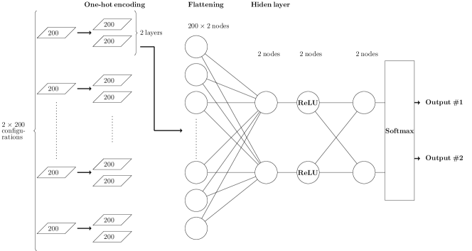
Figure 1: The MLP employed in this study.

II The considered models

The Hamiltonian of the 2D $q$-state clock model on the square lattice considered here has the following expression Cha18

$$H=-\sum_{\left<ij\right>}\vec{\sigma}_{i}\cdot\vec{\sigma}_{j},$$ (1)

where $\left<ij\right>$ refers to nearest neighbor sites $i$ and $j$, and $\vec{\sigma}_{i}$ is a vector at site $i$ with $\vec{\sigma}_{i}=\left(\cos\theta_{i},\sin\theta_{i}\right)$. Here $\theta_{i}=\frac{2\pi k}{q}$ with $k=1,2,...,q-2,q-1$.

III The constructed NN

The supervised NN, namely a multilayer perceptron (MLP) is built using the keras and tensorflow kera ; tens . In addition, it has extremely simple architecture. Specifically, the constructed NN has only one input layer, one hidden layer of two neurons, and one output layer. The considered algorithm and optimizer are minibatch and adam (learning rate is set to 0.05), respectively. The activation function ReLU (softmax) is applied in the hidden (output) layer. The definitions of ReLU and softmax are given by

$$\text{ReLU}(x)=\text{max}(0,x),$$ (2)

$$\left(\text{softmax}(x)\right)_{i}=\frac{e^{x_{i}}}{\sum_{j}e^{x_{j}}}.$$ (3)

One-hot encoding, flattening, and $L_{2}$ regularization are used as well. Finally, the loss function considered is the categorical crossentropy $C$ which is defined as

$$C=-\frac{1}{n}\sum_{x}\sum_{j}^{2}y_{j}\ln a_{j},$$ (4)

where $n$ is the number of objects included in each batch and $a_{j}$ are the outcomes obtained after applying all the layers. Moreover, $x$ and $y$ are the training inputs and the corresponding designed labels, respectively.

Figure 1 is adopted from Ref. Pen22 and is the cartoon representation of the employed supervised NN.

The training of the supervised NN is conducted using 200 copies of two one-dimensional artificially made configurations (Each of which consists of 200 sites) as the training set. These configurations contain no information from the considered models. Specifically, one (the other) configuration has 1 (0) as the values for all of its elements. Due to the used training set, the labels employed are two-component vectors (0,1) and (1,0). On a server with two opteron 6344 and 96G memory, the training takes only 24 seconds.

IV Numerical Results

IV.1 Preparation of configurations for the NN prediction

Using the Wolff algorithm Wol89 , we have generated several thousand configurations for the 6- and 8-state clock models with various temperatures $T$ and linear system sizes $L$. For each produced clock configuration, the angles $\theta$ of 2000 sites, which are randomly chosen, are stored. From these stored variables, two hundred are picked randomly and the resulting $\theta\,\,\text{mod}\,\,\pi$ are used to build a 1D configuration consisiting of 200 sites which will then be employed for the NN prediction.

IV.2 The NN results associated with 6-state clock model

The magnitude $R$ of the NN output vectors as functions of $T$ for various $L$ for the 6-state clock model are shown in fig. 2. The figure implies that there are possbily two phase transitions: one before and one after $T\sim 0.6$. The dashed vertical line is the expected transition temperature $T^{2}_{c}$ from LRO to PLRO. From the figure, one observes that there is a range of $T$ where data of various $L$ collapse to form a single (universal) curve. In addition, such a universal curve seems to end at $T^{2}_{c}$. This can be considered as a NN method of estimating $T^{2}_{c}$. Based on such an idea, the NN prediction for $T^{2}_{c}$ is found to be 0.67(2) (see fig. 3). The obtained $T^{2}_{c}$ agrees reasonably well with the MC result of 0.681 determined in Ref. Cha18 . It should be pointed out that this NN method of calculating $T^{2}_{c}$ is not of high precision. Despite this, it leads to a NN prediction of $T^{2}_{c}$ with acceptable quality.

After establishing a NN method of estimating $T^{2}_{c}$, we turn to the determination of the transition temperature $T^{1}_{c}$ from PLRO to paramagnetic phase. This transition is similar to that of the 2D classical $XY$ model. Hence we will use the standard analysis procedure to calculate $T^{1}_{c}$. First of all, one notices that $R$ will take the value of $1/\sqrt{2}\sim 0.70712$ at extremely high temperatures. As a result, for a given $L$, we will consider the intersection between the related $R$ data (as a function of $T$) and the curve of $2T/\pi q+0.70712$ with $q=6$ to be the estimated $T^{1}_{c}(L)$. With this approach, $T^{1}_{c}(L)$ as a function of $1/L$ is shown in fig. 4.

It is anticipated that the $T^{1}_{c}(L)$ should fulfill the following ansatz Nel77 ; Pal02

$$T^{1}_{c}(L)=T^{1}_{c}+\frac{b}{\left(\log\left(L\right)\right)^{2}},$$ (5)

where $b$ is some constant. A fit using the data of fig. 4 and above ansatz leads to $T^{1}_{c}=0.890(5)$. The obtained $T^{1}_{c}=0.890(5)$ agrees quantitatively with the expected $T^{1}_{c}\sim 0.892$.

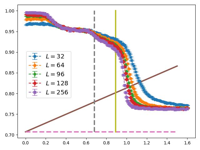
Figure 2: $R$ as functions of $T$ for various $L$ for the 6-state clock model. The dashed horizontal line is 0.70712. The vertical dashed and solid lines are the expected transition temperatures $T^{2}_{c}$ and $T^{1}_{c}$. The tilted line is $2T/(\pi q)+0.70712$ with $q=6$.

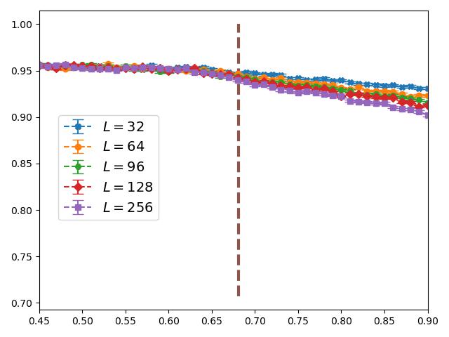
Figure 3: The smooth single (universal) curve formed by data collapse of various $L$ for the 6-state clock model. The vertical dashed line is the expected $T^{2}_{c}$.

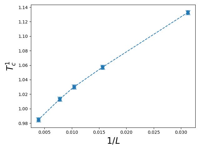
Figure 4: $T^{1}_{c}(L)$ as a function of $1/L$ for the 6-state clock model.

We would like to point out that analytically the finite-size scaling ansatz for the transition temperature $T_{\text{BKT}}$ of a BKT phase transition is given by

$$T_{\text{BKT}}(L)=T_{\text{BKT}}+a\frac{T_{\text{BKT}}}{\left(\log\left(L\right)+c\right)^{2}},$$ (6)

where $a$ and $c$ are some constants. A fit using this ansatz and the data of fig. 4 leads to $T^{1}_{c}=0.893(15)$ which also matches well with $T^{1}_{c}\sim 0.892$.

IV.3 The NN results associated with 8-state clock model

The magnitude $R$ of the NN output vectors as functions of $T$ for various $L$ for the 8-state clock model are shown in fig. 5. The conventions of the dashed and solid lines in the figure are similar to those used in fig 2. Following the same procedures for determining both the transition temperatures $T^{2}_{c}$ and $T^{1}_{c}$ of the 6-state clock model, the values of $T^{2}_{c}$ and $T^{1}_{c}$ for the 8-state clock model are calculated to be 0.40(2) and 0.884(7), respectively, sees figs. 6 and 7. We would like to point out that the tilted curve in fig. 5 is given by $2T/\left(\pi q\right)+0.70712$ with $q=8$ and $T^{1}_{c}=0.884(7)$ is obtained with data of $192\leq L\leq 1024$. The obtained $T^{2}_{c}=0.40(2)$ is in good agreement with $T^{2}_{c}=0.418$ found in Ref. Cha18 . Moreover, the determined $T^{1}_{c}$ of the 8-state clock model matches nicely with the expected $T^{1}_{c}\sim 0.892$ as well.

Finally, with a fit using equation (6) and data of fig. 7 ($64\leq L\leq 1024$), we arrive at $T^{1}_{c}=0.890(15)$.

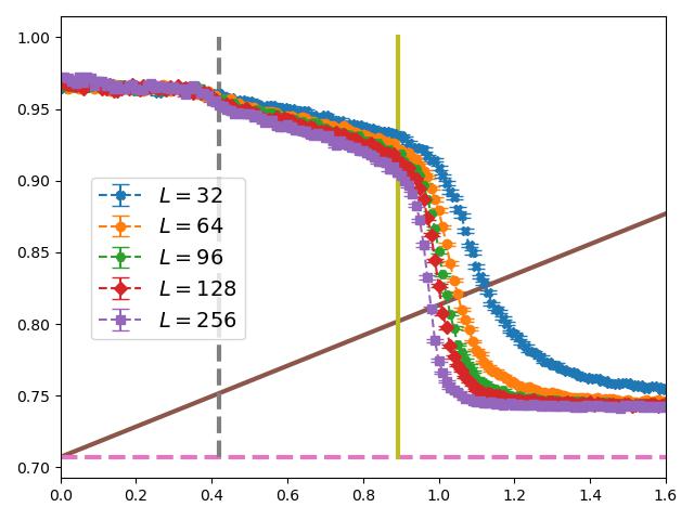
Figure 5: $R$ as functions of $T$ for various $L$ for the 8-state clock model. The dashed horizontal line is 0.70712. The vertical dashed and solid lines are the expected transition temperatures $T^{2}_{c}$ and $T^{1}_{c}$. The tilted line is $2T/(\pi q)+0.70712$ with $q=8$.

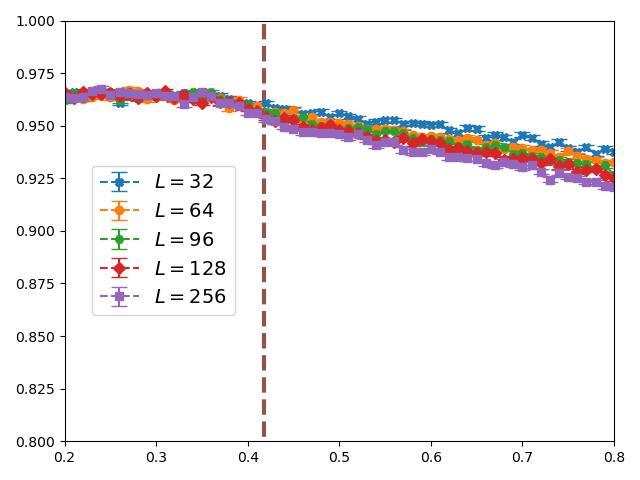
Figure 6: The smooth single (universal) curve formed by data collapse of various $L$ for the 8-state clock model. The vertical dashed line is the expected $T^{2}_{c}$.

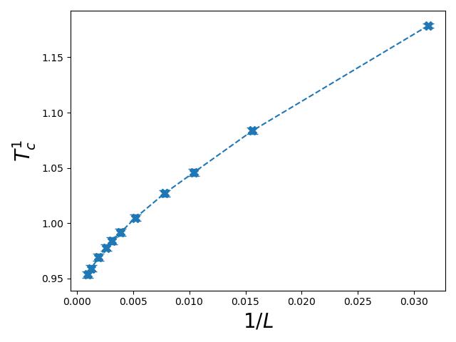
Figure 7: $T^{1}_{c}(L)$ as a function of $1/L$ for the 8-state clock model.

V Discussions and Conclusions

In this study, we calculate the transition temperatures $T^{1}_{c}$ and $T^{2}_{c}$ of the 6- and 8-state clock models using the technique of supervised NN. In particular, the employed supervised NN has extremely simple architecture, namely it consists of one input layer, one hidden layer of two neurons, and one output layer. The supervised NN is trained without any input from the considered models.

By considering the magnitude $R$ of the NN output vectors as functions of $T$ and $L$, the values of $T^{1}_{c}$ and $T^{2}_{c}$ are estimated using semi-experimental methods. The obtained NN outcomes of the transitions temperatures are in nice agreement with the corresponding results established in the literature.

Typically, one needs to construct a new NN whenever a new model or a different system size is considered. The outcomes shown in Refs. Tan21 ; Tse22 and here demonstrate that a NN with simple infrastructure can be recycled to investigate the phase transitions of many 3D and 2D models.

We would like to emphasize the fact that due to the unique features of the employed supervised NN, there is no system size restriction in our calculations. As a result, outcomes of $L=1024$ can be reached with ease.

In Refs. Bae09 ; Cha18 , two Binder ratios $U_{4}$ and $U_{m}$ are built to detect the the phase transitions associated with $T^{1}_{c}$ and $T^{2}_{c}$, respectively. It should be noticed that $U_{4}$ ($U_{m}$) cannot be used for studying the phase transition related to $T^{2}_{c}$ ($T^{1}_{c}$). Particularly, one needs to analytically investigate the model in order to construct the suitable observables to calculate the transition temperatures. For the present study, one single quantity, namely $R$ can reveal clear signals of both the transitions. The use of $R$ is natural and does not require any prior investigation of the targeted system(s). This feature can be considered as one advantage of our NN approach.

For the traditional methods, one can directly use the associated analytic predictions to perform the finite-size scaling analysis to extract the relevant physical quantities such as the critical points. For the NN method, such theoretical formulas typically do not exist and one has to rely on semi-experimental ansatzes to conduct the tasks. In particular, to establish these semi-experimental anstazes requires certain efforts of investigations, and the employed ansatzes may not be applicable to all cases. From this point of view, the NN method is still in the developing phase and there is room for improvement.

Finally, we would like to emphasize the fact that similar to the autoencoder and the generative adversarial network constructed in Ref. Tse22 , it is anticipated that the simple supervised NN employed in this study can be directly applied to study the phase transitions of other models, such as the three-dimensional (3D) $O(3)$ model, the 2D generalized $XY$ model, the one-dimensional (1D) Bose–Hubbard model, and the 2D $q$-state ferromagnetic Potts model. In other words, it is likely that one can construct a universal NN that is applicable to investigate the phase transitions of many systems.

References

- (1) V. L. Berezinskii, Destruction of long range order in one-dimensional and two-dimensional systems having a continuous symmetry group. I. Classical systems, Sov. Phys. JETP 32 (1971) 493.
- (2) V. L. Berezinskii, Destruction of Long-range Order in One-dimensional and Two-dimensional Systems Possessing a Continuous Symmetry Group. II. Quantum Systems, Sov. Phys. JETP 34 (1972) 610.
- (3) J. M. Kosterlitz and D. J. Thouless, Long range order and metastability in two dimensional solids and superfluids. (Application of dislocation theory), J. Phys. C 5 (1972) L124.
- (4) J. M. Kosterlitz and D. J. Thouless, Ordering, metastability and phase transitions in two-dimensional systems, J. Phys. C 6 (1973) 1181.
- (5) J. M. Kosterlitz, The critical properties of the two-dimensional xy model, J. Phys. C 7 (1974) 1046.
- (6) J. V. José, L. P. Kadanoff, S. Kirkpatrick, and D. R. Nelson, Renormalization, vortices, and symmetry-breaking perturbations in the two-dimensional planar model, Phys. Rev. B 16, 1217 (1977).
- (7) J. L. Cardy, General discrete planar models in two dimensions: Duality properties and phase diagrams, J. Phys. A 13, 1507 (1980).
- (8) H. H. Roomany and H. W. Wyld, Finite-lattice Hamiltonian results for the phase structure of the models and the -state Potts models, Phys. Rev. B 23, 1357 (1981).
- (9) J. Tobochnik, Properties of the -state clock model for and 6 , Phys. Rev. B 26, 6201 (1982).
- (10) Y. Tomita and Y. Okabe, Probability-Changing Cluster Algorithm for Potts Models , Phys. Rev. Lett. 86, 572 (2001).
- (11) Y. Tomita and Y. Okabe, Probability-changing cluster algorithm for two-dimensional and clock models, Phys. Rev. B 65, 184405 (2002).
- (12) Y. Tomita and Y. Okabe, Finite-size scaling of correlation ratio and generalized scheme for the probability-changing cluster algorithm, Phys. Rev. B 66, 180401(R) (2002).
- (13) T. Surungan and Y. Okabe, Kosterlitz-Thouless transition in planar spin models with bond dilution, Phys. Rev. B 71, 184438 (2005).
- (14) C. M. Lapilli, P. Pfeifer, and C. Wexler, Universality Away from Critical Points in Two-Dimensional Phase Transitions, Phys. Rev. Lett. 96, 140603 (2006).
- (15) S. K. Baek, P. Minnhagen, and B. J. Kim, True and quasi-long- range order in the generalized q-state clock model, Phys. Rev. E 80, 060101(R) (2009).
- (16) S. K. Baek, P. Minnhagen, and B. J. Kim, Comment on “Six-state clock model on the square lattice: Fisher zero approach with Wang-Landau sampling”, Phys. Rev. E 81, 063101 (2010).
- (17) Raymond P. H. Wu, V.-c. Lo, and H. Huang, Critical behavior of two-dimensional spin systems under the random-bond six-state clock model, J. Appl. Phys. 112, 063924 (2012).
- (18) G. Ortiz, E. Cobanera, and Z. Nussinov, Dualities and the phase diagram of the p-clock model, Nucl. Phys. B 854, 780 (2012).
- (19) Y. Kumano, K. Hukushima, Y. Tomita, and M. Oshikawa, Response to a twist in systems with symmetry: The two- dimensional p-state clock model, Phys. Rev. B 88, 104427 (2013).
- (20) S. Chatterjee, S. Puri, and R. Paul, Ordering kinetics in the q- state clock model: Scaling properties and growth laws, Phys. Rev. E 98, 032109 (2018).
- (21) T. Surungan, S. Masuda, Y. Komura, and Y. Okabe, Berezinskii- Kosterlitz-Thouless transition on regular and Villain types of - state clock models, J. Phys. A: Math. Theor. 52, 275002 (2019).
- (22) Matthias Rupp, Alexandre Tkatchenko, Klaus-Robert Müller, and O. Anatole von Lilienfeld, Fast and Accurate Modeling of Molecular Atomization Energies with Machine Learning, Phys. Rev. Lett. 108 058301 (2012).
- (23) John C. Snyder, Matthias Rupp, Katja Hansen, Klaus-Robert Müller, and Kieron Burke, Finding Density Functionals with Machine Learning, Phys. Rev. Lett. 108 253002 (2012).
- (24) P. Baldi, P. Sadowski and D. Whiteson, Enhanced Higgs Boson to Search with Deep Learning, Phys. Rev. Lett. 114, 111801 (2015).
- (25) V. Mnih, K. Kavukcuoglu, D. Silver, A. A. Rusu, J. Veness, M. G. Bellemare, A. Graves, M. Riedmiller, A. K. Fidjeland, G. Ostrovski, S. Petersen, C. Beattie, A. Sadik, I. Antonoglou, H. King, D. Kumaran, D. Wierstra, S. Legg and D. Hassabis, Human-level control through deep reinforcement learning, Nature 518, no.7540, 529-533 (2015).
- (26) Tomoki Ohtsuki and Tomi Ohtsuki, Deep Learning the Quantum Phase Transitions in Random Two-Dimensional Electron Systems, J. Phys. Soc. Jpn. 85, 123706 (2016).
- (27) B. Hoyle, Measuring photometric redshifts using galaxy images and Deep Neural Networks, Astron. Comput. 16, 34-40 (2016).
- (28) Juan Carrasquilla, Roger G. Melko, Machine learning phases of matter, Nature Physics 13, 431–434 (2017).
- (29) Evert P.L. van Nieuwenburg, Ye-Hua Liu, Sebastian D. Huber, Learning phase transitions by confusion, Nature Physics 13, 435–439 (2017).
- (30) Dong-Ling Deng, Xiaopeng Li, and S. Das Sarma, Machine learning topological states, Phys. Rev. B 96 195145 (2017).
- (31) Wenjian Hu, Rajiv R. P. Singh, and Richard T. Scalettar, Discovering phases, phase transitions, and crossovers through unsupervised machine learning: A critical examination, Phys. Rev. E 95, 062122 (2017).
- (32) C.-D. Li, D.-R. Tan, and F.-J. Jiang, Applications of neural networks to the studies of phase transitions of two-dimensional Potts models, Annals of Physics, 391 (2018) 312-331.
- (33) Kelvin Ch’ng, Nick Vazquez, and Ehsan Khatami, Unsupervised machine learning account of magnetic transitions in the Hubbard model, Phys. Rev. E 97, 013306 (2018).
- (34) Lu, S., Zhou, Q., Ouyang, Y. et al., Accelerated discovery of stable lead-free hybrid organic-inorganic perovskites via machine learning, Nat Commun 9, 3405 (2018).
- (35) Keith T. Butler, Daniel W. Davies, Hugh Cartwright, Olexandr Isayev, and Aron Walsh, Machine learning for molecular and materials science, Nature 559, 547–555 (2018).
- (36) Phiala E. Shanahan, Daniel Trewartha, and William Detmold, Machine learning action parameters in lattice quantum chromodynamics, Phys. Rev. D 97, 094506 (2018).
- (37) Joaquin F. Rodriguez-Nieva and Mathias S. Scheurer, Identifying topological order through unsupervised machine learning, Nat. Phys. 15, 790–795 (2019).
- (38) Wanzhou Zhang, Jiayu Liu, and Tzu-Chieh Wei, Machine learning of phase transitions in the percolation and XY models, Phys. Rev. E 99, 032142 (2019).
- (39) D.-R. Tan et al. A comprehensive neural networks study of the phase transitions of Potts model, 2020 New J. Phys. 22 063016.
- (40) D.-R. Tan and F.-J. Jiang, Machine learning phases and criticalities without using real data for training, Phys. Rev. B 102, 224434 (2020).
- (41) A. J. Larkoski, I. Moult and B. Nachman, Jet Substructure at the Large Hadron Collider: A Review of Recent Advances in Theory and Machine Learning, Phys. Rept. 841, 1-63 (2020).
- (42) G. Aad et al. [ATLAS], Dijet resonance search with weak supervision using TeV collisions in the ATLAS detector, Phys. Rev. Lett. 125, no.13, 131801 (2020).
- (43) K. A. Nicoli, C. J. Anders, L. Funcke, T. Hartung, K. Jansen, P. Kessel, S. Nakajima and P. Stornati, Estimation of Thermodynamic Observables in Lattice Field Theories with Deep Generative Models, Phys. Rev. Lett. 126, no.3, 032001 (2021).
- (44) Yusuke Miyajima, Yusuke Murata, Yasuhiro Tanaka, and Masahito Mochizuki, Machine learning detection of Berezinskii-Kosterlitz-Thouless transitions in -state clock models, Phys. Rev. B 104, 075114 (2021).
- (45) D.-R. Tan, J.-H. Peng, Y.-H. Tseng, F.-J. Jiang, A universal neural network for learning phases, Eur. Phys. J. Plus 136 (2021) 11, 1116.
- (46) Yuan-Heng Tseng, Fu-Jiun Jiang, and C.-Y. Huang, A universal training scheme and the resulting universality for machine learning phases, Prog. Theor. Exp. Phys. 2023 013A03.
- (47) Jhao-Hong Peng, Yuan-Heng Tseng, Fu-Jiun Jiang, arXiv:2212.14655.
- (48) https://keras.io
- (49) https://www.tensorflow.org
- (50) U. Wolff, Collective Monte Carlo Updating for Spin Systems, Phys. Rev. Lett. 62, 361 (1989).
- (51) D. R. Nelson and J. M. Kosterlitz, Universal Jump in the Superfluid Density of Two-Dimensional Superfluids, Phys. Rev. Lett. 39, 1201 (1977).
- (52) G. Palma, T. Meyer, and R. Labbé, Finite size scaling in the two-dimensional model and generalized universality, Phys. Rev. E 66, 026108 (2002).