Low–Energy Deuteron–Alpha Elastic Scattering in Cluster Effective Field Theory

Abstract

In this paper, we study the low-energy $d-\alpha$ elastic scattering within the two-body cluster effective field theory (EFT) framework. The importance of the $d(\alpha,\alpha)d$ scattering in the ${}^{6}\textrm{Li}$ production reaction leads us to study this system in an effective way. In the beginning, the scattering amplitudes of each channel are written in a cluster EFT with two-body formalism. Using the effective range expansion analysis for the elastic scattering phase shift of $S$, $P$ and $D$ partial waves, the unknown EFT low-energy coupling constants are determined and the leading and next-to-leading orders EFT results for the phase shift in each channel are presented. To verify the accuracy of the results, we compare experimental phase shift and differential cross section data with obtained results. The accuracy of the EFT results and consistency with the experimental data indicate that the EFT is an effective approach for describing low-energy systems.
Keywords. Cluster Effective Field Theory, Elastic Scattering, Coulomb Interaction, Phase Shifts.
PACS. 21.45-v Few-body systems - 11.10.-z Field theory - 03.65.Nk Scattering theory

I Introduction

The $d-\alpha$ elastic scattering has been of interest for many years as a source of information about the low-lying $T\!=\!0$ states of ${}^{6}\textrm{Li}$. The analysis of $d-\alpha$ elastic scattering data, to obtain the correct energy dependent phase shifts of this process and determine the corresponding level parameters of the ${}^{6}\textrm{Li}$ nucleus, has been studied widely in the past decades. The $d-\alpha$ scattering has been studied extensively in the pastL. C. Mc lntyre ; A. Jenny ; P. Marmier ; W. Gr ; M. Bruno ; I. Koersner ; I. Slaus ; P. Niessen ; Y. Koike ; K. Hahn ; A. Galonsky , and the low-lying levels of ${}^{6}\textrm{Li}$ have been extensively investigated both experimentally and theoretically L. S. Senhouse ; K. W. Allen ; W. C. Barber ; T. A. Romanowski ; D. R. Inglis ; P. H. Wackman . Recently, the $d-\alpha$ scattering was investigated using the screening and renormalization approach in the framework of momentum space three-particle equations A. Deltuva .

In the present work, we focus on applying the effective field theory (EFT) formalism as a model-independent, systematic and controlled-precision procedure for the investigation of $d-\alpha$ elastic scattering at the center-of-mass (CM) energies about a few MeV corresponding to the validity of the EFT expansion. The applications of EFT approach in the few-nucleon systems have been widely studied Bedaque-van Kolck ; Braaten-Hammer ; Kaplan-S-W ; Phillips-R-S ; Chen-R-S . Also, in recent years the nuclear systems with $A\!>\!4$ which can be classified in the two-body sector are studied by halo EFT scheme Hammer-Phillips . The deuteron can be thought of as the simplest halo nucleus whose core is a nucleon, however, there are some EFT works that the deuteron field is introduced as an elementary-like field Ando-nd ; Ando-Yang-Oh ; MMA-dt-na ; MMA-dt-dt . Halo EFT captures the physics of resonantly $P$-wave interactions in $n-\alpha$ scattering up to next-to-leading order (NLO) bertulani-et al ; Bedaque-et al and studying two-neutron halo system ⁶He chen-ji ; MMA-nna . The effects of the Coulomb interaction in two-body systems such as $p-$$p$ 33 ; Kong-Ravndal01 ; Barford-Birse ; Ando-S-H-H ; Ando-Birse , $p-$⁷Li Lensky-Birse , $\alpha-$${}^{12}\textrm{C}$ Ando-12C , and $\alpha-\alpha$ scattering Higa-Hammer and ³$\textrm{He}(\alpha,\gamma)^{7}$Be Higa-Rupak-Vaghani , have been considered by the EFT approach.

Before applying the EFT method to the description of low-energy $d-\alpha$ radiative capture, we construct the EFT formalism for the $d-\alpha$ scattering in the current study. Although $d-\alpha$ is a six-nucleon system, at low energies, to a good approximation, the alpha particle may be considered a spin zero structureless boson, and thereby the theoretical description of $d-\alpha$ scattering may be reduced to a three-body problem made up of one alpha and two nucleons. At the low-energy regime below deuteron breakup, we can take into account that both deuteron and alpha nucleus as point-like and structureless particles. Therefore, our present EFT for low-energy $d-\alpha$ scattering is constructed using the two-body cluster formalism. The phase shift analysis and differential cross section calculation for the elastic $d-\alpha$ scattering procedure, after determination of the unknown EFT low-energy coupling constants (LECs), are the main purposes of this paper. We obtain the EFT LECs by using available low-energy experimental data for the elastic $d-\alpha$ scattering. Here, we study the scattering into the $S$-, $P$- and $D$-wave states using the effects corresponding to the scattering length, effective range and shape parameter at each channel. The evaluated results can help us to investigate the astrophysical radiative capture processes $d+\alpha\rightarrow^{6}$$\textrm{Li}+\gamma$ using halo/cluster EFT formalism in the future.

The manuscript is organized as follows. In Sec. II, the pure Coulomb and Coulomb-subtracted amplitudes of the $d-\alpha$ scattering in all possible $l\!=\!0,~{}1,~{}2$ partial waves using the effective range expansion (ERE) and EFT formalisms are calculated. The values of the unknown EFT LECs are determined by matching our relations of phase shift to the available low-energy experimental data in Sec. III. Using the power counting analysis of the effective range parameters, we plot the EFT differential cross section against CM energy and angle with the dominant scattering amplitudes and compare with the available data in Sec. IV. We summarize the paper and discuss extension of the investigation to other few-body systems in Sec. V.

II Scattering amplitude

In this section, the pure Coulomb and Coulomb-subtracted scattering amplitudes for the two-body $d-\alpha$ elastic scattering using cluster EFT formalism are extracted. The elastic scattering amplitude for two particles interacting via short-range strong and long-range Coulomb interactions in the CM framework is written as

$$T(\textbf{p}^{\prime},\textbf{p};E)=T_{C}(\textbf{p}^{\prime},\textbf{p};E)+T_{CS}(\textbf{p}^{\prime},\textbf{p};E),$$ (1)

where $T_{C}$ indicates the pure Coulomb scattering amplitude and $T_{CS}$ represents the scattering amplitude for the strong interaction in the presence of the Coulomb interaction with $E\!=\!\frac{p^{2}}{2\mu}$ as the CM energy of the system. p and $\textbf{p}^{\prime}$ denote the relative momentum of incoming and outgoing particles, respectively Higa-Hammer .

II.1 Pure Coulomb amplitude

.

The strength of the Coulomb-photon exchanges is provided by the dimensionless Sommerfeld parameter which for the $d-\alpha$ interaction can be written as

$$\eta_{p}=\frac{k_{C}}{p}=\frac{Z_{\alpha}Z_{d}\,\alpha_{em}\,\mu}{p}.$$ (2)

Here $k_{C}$ is the inverse of the Bohr radius of the $d-\alpha$ system, $\alpha_{em}\!\equiv\!e^{2}/4\pi\!\sim\!1/137$ represents the fine structure constant, $p$ is the relative momentum of two particles in the CM framework, $Z_{\alpha}(Z_{d})$ indicates the atomic numbers of alpha (deuteron), and $\mu$ denotes the reduced mass of $d-\alpha$ system. Based on the fact that each photon-exchange insertion is proportional to $\eta_{p}$ so, in the low-energy scattering region, $p\lesssim k_{C}$, we should consider the full Coulomb interaction non-perturbatively as depicted in Fig. 1. In order to consider the Coulomb contribution in the two-body $d-\alpha$ system, we use the Coulomb Green’s function as follows. According to Fig. 1, the Coulomb Green’s function is related to the free Green’s function through the integral equation as goldberger1964collision

$$\hat{G}_{C}^{\pm}=\hat{G}_{0}^{\pm}+\hat{G}_{0}^{\pm}\,\hat{V}_{C}\,\hat{G}_{C}^{\pm},$$ (3)

where the free and Coulomb Green’s functions for the $d-\alpha$ system are given by

$$\hat{G}_{0}^{\pm}=\frac{1}{E-\hat{H}_{0}\pm i\epsilon},\quad\quad\hat{G}_{C}^{\pm}=\frac{1}{E-\hat{H}_{0}-\hat{V}_{C}\pm i\epsilon},$$ (4)

with $\hat{V}_{C}\!=\!2\alpha_{em}/r$ and $\hat{H}_{0}\!=\!\frac{\hat{p}^{2}}{2\mu}$ as the repulsive Coulomb potential between alpha and deuteron and the free-particle Hamiltonian, respectively. The signs $(\pm)$ are corresponding to the retarded and advanced Green’s functions. The incoming and outgoing Coulomb wave functions can be obtained by solving the Schrodinger equation with the full Hamiltonian $\hat{H}\!=\!\hat{H}_{0}\!+\!\hat{V}_{C}$ as 33 ; holstein1999hadronic

$$\chi_{p}^{(\pm)}(\textbf{r})=\sum_{l=0}^{\infty}(2l+1)i^{l}e^{i\sigma_{l}}P_{l}(\hat{\textbf{p}}\cdot\hat{\textbf{r}})\,C_{l}(\eta_{p})\,(rp)^{l}e^{\mp i\textbf{p}\cdot\textbf{r}}\textrm{M}(l+1\pm i\eta_{p},2l+2;\pm 2ipr),\quad$$ (5)

where $\textrm{M}(a,b;z)$ is well-known Kummer function, $P_{l}$ denotes the Legendre function and $\sigma_{l}\!=\!\arg\mathrm{\Gamma}(l+1+i\eta_{p})$ indicates the pure Coulomb phase shift abromowitz1965handbook . The normalized constant $C_{l}(\eta_{p})$ is always positive and has the form

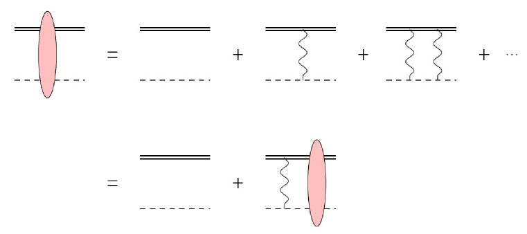
Figure 1: Coulomb ladder diagrams. The single dashed and double lines represent the scalar $\alpha$ and vector deuteron particle, respectively. The wavy lines represent the exchanged photons.

$$C^{2}_{l}(\eta_{p})=\frac{2^{2l}C_{0}^{2}(\eta_{p})\,\prod_{n=1}^{l}(n^{2}+\eta_{p}^{2})}{\mathrm{\Gamma}(2l+2)^{2}},$$ (6)

where $C_{0}^{2}(\eta_{p})$, the probability to find the two interacting particles at zero separation, is defined as

$$C_{0}^{2}(\eta_{p})=\chi_{p^{\prime}}^{(\pm)}(\mathbf{0})\chi_{p}^{*(\pm)}(\mathbf{0})=\frac{2\pi\eta_{p}}{e^{2\pi\eta_{p}}-1}.$$ (7)

According to the expression of the Coulomb wave function of Eq. (5), the partial wave expansion of the pure Coulomb amplitude is given by gaspard2018connection

$$T_{C}(\textbf{p}^{\prime},\textbf{p};E) = \langle\mathbf{p}^{\prime}|\hat{V}_{C}|\chi_{p}^{(+)}\rangle=\sum_{l=0}^{\infty}(2l+1)T_{C}^{[l]}P_{l}(\hat{\mathbf{p}}^{\prime}\cdot\hat{\mathbf{p}})$$ (8)

$$= -\frac{2\pi}{\mu}\sum_{l=0}^{\infty}(2l+1)\frac{e^{2i\sigma_{l}}-1}{2ip}P_{l}(\hat{\mathbf{p}}^{\prime}\cdot\hat{\mathbf{p}})$$

$$= \frac{2\pi}{\mu}\frac{\eta_{p}^{2}}{2k_{C}}\,\csc^{2}(\theta/2)\,\textrm{exp}\big{[}2i\sigma_{0}-2i\eta_{p}\,\ln(\sin(\theta/2))\big{]},\qquad$$

where $\cos\theta=\hat{\mathbf{p}}^{\prime}\cdot\hat{\mathbf{p}}$ and $p=|\mathbf{p}|=|\mathbf{p}^{\prime}|$. This is the well-known Mott scattering amplitude which holds at very low energies bethe1949theory .

II.2 Coulomb-subtracted scattering amplitude

The strong scattering amplitude modified by the Coulomb corrections is

$$T_{CS}(\mathbf{p}^{\prime},\mathbf{p};E)=\langle\chi_{p^{\prime}}^{(-)}|\hat{V}_{S}|\mathrm{\Psi}_{p}^{(+)}\rangle,$$ (9)

where $|\mathrm{\Psi}_{p}^{(+)}\rangle$ represent incoming state for Coulomb-distorted short-range interaction, while $\hat{V}_{S}$ is the short-range interaction operator. The amplitude $T_{CS}$ can be expressed in the partial wave decomposition as 33

$$T_{CS}(\mathbf{p}^{\prime},\mathbf{p};E)=\sum_{l=0}^{\infty}(2l+1)T^{[l]}_{CS}(p)\,e^{2i\sigma_{l}}P_{l}(\mathbf{p}^{\prime}\cdot\mathbf{p}),$$ (10)

with

$$T^{[l]}_{CS}(p) = -\frac{2\pi}{\mu}\frac{1}{p(\textrm{cot}\delta_{l}-i)},\quad\quad\,\,\,$$ (11)

where $\delta_{l}$ denotes the Coulomb-corrected phase shift. The Coulomb-subtracted amplitude $T^{[l]}_{CS}$ can usually be expressed in terms of a modified ERE as Ando-12C

$$T^{[l]}_{CS}(p) = -\frac{2\pi}{\mu}\frac{C_{0}^{2}(\eta_{p})\,W_{l}(\eta_{p})}{K_{l}(p)-H_{l}(\eta_{p})},\quad$$ (12)

with

$$W_{l}(\eta_{p}) = \frac{k_{C}^{2l}}{(l!)^{2}}\,\prod^{l}_{n=0}(1+\frac{n^{2}}{\eta_{p}^{2}}),$$ (13)

$$H_{l}(\eta_{p}) = 2k_{C}W_{l}(\eta_{p})H(\eta_{p}),$$ (14)

$$H(\eta_{p}) = \psi(i\eta_{p})+\frac{1}{2i\eta_{p}}-\ln(i\eta_{p}),$$ (15)

where the function $\psi$ is the logarithmic derivative of Gamma function. The function $K_{l}(p)$ represents the interaction due to the short-range strong interaction which is obtained in terms of the effective range parameters as bethe1949theory

$$K_{l}(p) = -\frac{1}{a_{l}}+\frac{1}{2}r_{l}\,p^{2}+\frac{1}{4}s_{l}\,p^{4}+\cdots,$$ (16)

with $a_{l}$, $r_{l}$ and $s_{l}$ as the scattering length, effective range and shape parameter, respectively.

II.3 Scattering amplitudes in cluster EFT approach

In the present study, we consider the deuteron and alpha as the point-like particles, so the degrees of freedom of the $d-\alpha$ system in the current cluster EFT are only alpha and deuteron. At the low-energy regime, the $S$, $P$ and $D$ partial waves have the dominant contributions in the $d-\alpha$ elastic scattering amplitude. We should point out that the available low-energy experimental data for the differential cross section of the elastic $d-\alpha$ scattering show a resonance below the CM energy 1 MeV. Theoretically, this resonance can be constructed only by including the $D$-wave effects in the cross section. Also, the dominant contribution of the deuteron radiative capture by alpha particles at energy above 0.5 MeV comes from E2 transition with incoming $D$-wave states Higa-Hammer ; Andophys2006 ; braun2019electric . Therefore, we consider the $D$-wave scattering amplitudes of the $d-\alpha$ system in the present low-energy study. So, according to the spin zero of alpha and spin one of the deuteron and considering the $l$-wave components of the $d-\alpha$ system, the possible states for the two-body $d-\alpha$ system are $\xi\equiv$ ${}^{3}\!S_{1}$, ${}^{3}\!P_{0}$, ${}^{3}\!P_{1}$, ${}^{3}\!P_{2}$, ${}^{3}\!D_{1}$, ${}^{3}\!D_{2}$ and ${}^{3}\!D_{3}$ corresponding to the total angular momentums, $J=0,1,2,3$.

At the low-energy regime, $p\!\leq\!k_{C}\sim 18~{}\textrm{MeV}$, the on-shell CM momentum of the system is scaled as low-momentum $Q$. The high-momentum scale is set by the lowest energy degrees of freedom that has been integrated out. According to the fact that there is no existing explicit pions and any deuteron deformation, the high-momentum scale $\mathrm{\Lambda}$ has been chosen between the pion mass, $m_{\pi}\sim 140$ MeV and the momentum corresponding to the deuteron binding energy, $B_{d}$ i.e., $\sqrt{2m_{d}B_{d}}\sim 90$ MeV. Around the $p\sim k_{C}\sim 18$ MeV, the expansion parameter of the current EFT is estimated of the order $1/5$. Increasing the energy, the expansion deteriorates and the precision of our EFT prediction will be questionable for $E_{CM}=\frac{p^{2}}{2\mu}>3.3$ MeV. The Sommerfeld parameter $\eta_{p}$ is enhanced by decreasing the energy. So, $\eta_{p}$ would be large around $p\!\lesssim\!k_{C}$ and the elastic scattering amplitude requires non-perturbative treatment of the Coulomb photons.

The non-relativistic Lagrangian for the strong interactions in the $d-\alpha$ system involving the invariance under small-velocity Lorentz, parity and time-reversal transformations and describing the dynamics in all feasible channels is given by

$$\mathcal{L}^{[\xi]} = \phi^{\dagger}(i\partial_{0}+\frac{\nabla^{2}}{2m_{\alpha}})\phi+d_{i}^{\dagger}(i\partial_{0}+\frac{\nabla^{2}}{2m_{d}})d_{i}+\,\eta^{[\xi]}t^{[\xi]^{\dagger}}\!\Big{[}i\partial_{0}\!+\!\frac{\nabla^{2}}{2m_{t}}-\mathrm{\Delta}^{[\xi]}\Big{]}\!t^{[\xi]}$$ (17)

$$+\,g^{[\xi]}[t^{[\xi]^{\dagger}}\!(\phi\,\mathrm{\Pi}^{[\xi]}d)+h.c.]+\,h^{[\xi]}t^{[\xi]^{\dagger}}\!\Big{[}(i\partial_{0}\!+\!\frac{\nabla^{2}}{2m_{t}})^{2}\Big{]}t^{[\xi]}+\cdots,$$

where ”$\cdots$” stands for the terms with more derivatives and/or auxiliary fields. The scalar field $\phi$ represents the spinless $\alpha$ field with mass $m_{\phi}\!=\!3727.38~{}\textrm{MeV}$ and the vector field $d_{i}\!=\!\varepsilon_{i}^{d}d$ indicates the deuteron nucleus axillary field with mass $m_{d}\!=\!1875.61~{}\textrm{MeV}$. The sign $\eta^{[\xi]}$ is used to match the sign of the effective range $r^{[\xi]}$ and reflects the auxiliary character of the dimeron field. The dimeron field $t^{[\xi]}$ with mass $m_{t}\!=\!m_{d}\!+\!m_{\phi}$, and ${\mathrm{\Pi}}^{[\xi]}$ operator for each $\xi$ channel are defined as

$$t^{[\xi]} = \left\{\begin{array}[]{lc}\bar{t}_{i},&\qquad\qquad\quad\,\xi={{}^{3}\!S_{1}}\\ t,&\,\qquad\qquad\quad\xi={{}^{3}\!P_{0}}\\ t_{k},&\,\qquad\qquad\quad\xi={{}^{3}\!P_{1}}\\ t_{ij},&\,\qquad\qquad\quad\xi={{}^{3}\!P_{2}}\\ \tilde{t}_{j},&\,\qquad\qquad\quad\xi={{}^{3}\!D_{1}}\\ \tilde{t}_{kl},&\,\qquad\qquad\quad\xi={{}^{3}\!D_{2}}\\ \tilde{t}_{kji},&\,\qquad\qquad\quad\xi={{}^{3}\!D_{3}}\!\!\end{array}\right\},\,\qquad$$ (25)

$$\mathrm{\Pi}^{{[\xi]}} = \left\{\begin{array}[]{lc}\varepsilon_{i}^{d},&\,\xi={{}^{3}\!S_{1}}\\ \sqrt{3}\,\mathcal{P}_{i}\,\varepsilon_{i}^{d},&\,\xi={{}^{3}\!P_{0}}\\ \sqrt{3/2}\,\epsilon_{kji}\,\mathcal{P}_{j}\,\varepsilon_{i}^{d},&\,\xi={{}^{3}\!P_{1}}\\ 3/\sqrt{5}\,\mathcal{P}_{j}\,\varepsilon_{i}^{d},&\,\xi={{}^{3}\!P_{2}}\\ 3/\sqrt{2}\,\tau_{ji}\,\varepsilon_{i}^{d},&\,\xi={{}^{3}\!D_{1}}\\ \sqrt{3/2}\,\epsilon_{ijl}\,\tau_{kj}\,\varepsilon_{i}^{d},&\,\xi={{}^{3}\!D_{2}}\\ \sqrt{45/8}\,\tau_{kj}\,\varepsilon_{i}^{d},&\,\xi={{}^{3}\!D_{3}}\end{array}\right\},\,\,\,\qquad$$ (33)

where the derivative operators are introduced as

$$\mathcal{P}_{i}=\frac{1}{i}(\frac{\mu}{\overrightarrow{m}}\overrightarrow{\nabla_{i}}-\frac{\mu}{\overleftarrow{m}}\overleftarrow{\nabla_{i}}),\quad\,\tau_{ij}=\mathcal{P}_{i}\mathcal{P}_{j}-\frac{1}{3}\delta_{ij}\mathcal{P}_{k}\mathcal{P}_{k}.\quad$$ (34)

In the following, the coupling constants $\mathrm{\Delta}^{[\xi]}$, $g^{[\xi]}$, and $h^{[\xi]}$ for channel $\xi$ are related to the corresponding scattering length, effective range and shape parameter.

The cluster EFT diagram of the $d-\alpha$ elastic scattering amplitude is shown in Fig. 2. According to this diagram the building block of the scattering amplitude is the full propagator of the dimeron. The bare and full propagators used in $T_{CS}^{[\xi]}(\mathbf{p}^{\prime},\mathbf{p},E)$ are depicted by the thick line and the thick line with filled circle, respectively. To evaluate the EFT results for the $d-\alpha$ elastic scattering amplitude in channel $\xi$, the external legs should be attached to the full dimeron propagator as shown in the first line of Fig. 2. So, the Coulomb-subtracted EFT amplitudes of the on-shell $d-\alpha$ scattering for each channel $\xi$ can be evaluated by

$$-i(2l+1)T_{CS}^{[\xi]}(p)P_{l}(\hat{\textbf{p}}^{\prime}\cdot\hat{\textbf{p}})e^{2i\sigma_{l}}=-ig^{[\xi]^{2}}D^{[\xi]}(E,\textbf{0})C^{2}_{0}(\eta_{p})W_{l}(\eta_{p})P_{l}(\hat{\textbf{p}}^{\prime}\cdot\hat{\textbf{p}})e^{2i\sigma_{l}}\quad\quad.$$ (35)

The detailed derivations of Eq. (35) for all channels are presented in Appendix A.

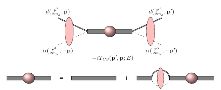
Figure 2: The amplitude of the $d-\alpha$ elastic scattering. The thick line is the bare dimeron propagator and the thick dashed line with a filled circle represents the full dimeron propagator. All remained notations are the same as in Fig. 1.

Here, without any estimation for the values of effective range parameters, we introduce the initial scheme in which the LO contribution of Coulomb-subtracted $d-\alpha$ scattering for channels $\xi\equiv$ ${}^{3}\!S_{1}$, ${}^{3}\!P_{0}$, ${}^{3}\!P_{1}$, and ${}^{3}\!P_{2}$ are calculated using the first four terms in Lagrangian (17) and the last term initially enters as NLO corrections as in some literature on the halo/cluster EFT Hammer-Phillips ; rupak2016radiative ; ryberg2014effective . However, the properties of the $D$-wave states are somewhat different. For the LO calculation of the $D$ waves, taking into account $\eta^{[\xi]}\!=\!\pm 1$, we should include three EFT LECs in our Lagrangian (17), namely, $\mathrm{\Delta}^{[\xi]}$, $g^{[\xi]}$, and $h^{[\xi]}$ corresponding to the scattering length, effective range, and shape parameter. The additional second-order kinetic term constant $h^{[\xi]}$ is needed to renormalize the interacting $D$-wave propagator which contains up to quintic divergences braun2019electric . According to this suggested scheme, the LO contribution of the scattering amplitude in channels $\xi={{}^{3}\!S_{1}},$ ${{}^{3}\!P_{0}}$, ${{}^{3}\!P_{1}}$, and ${{}^{3}\!P_{2}}$ is constructed by both their scattering lengths and effective ranges and their shape parameter influences are considered as NLO correction. However, for $\xi={{}^{3}\!D_{1}},$ ${{}^{3}\!D_{2}}$, and ${{}^{3}\!D_{3}}$ channels, all the scattering lengths, effective ranges, and shape parameters insert in the scattering amplitude at LO.

So, with respect to Fig. 2, up-to-NLO full dimeron propagator for $l\!=\!0$ and 1 channels in the CM framework can be evaluated by

$$D^{[\xi]}(E,\textbf{0}) = \frac{\eta^{[\xi]}}{E\!-\!\mathrm{\Delta}^{[\xi]}-\!\frac{1}{2l+1}\eta^{[\xi]}g^{[\xi]^{2}}J_{l}(E)}\Big{[}\underbrace{\!\!\!1\!\!\!\!}_{\mathrm{LO}}\!\!-\underbrace{\frac{\eta^{[\xi]}h^{[\xi]}E^{2}}{E\!-\!\mathrm{\Delta}^{[\xi]}-\!\frac{1}{2l+1}\eta^{[\xi]}g^{[\xi]^{2}}J_{l}(E)}}_{\mathrm{NLO~{}corection}}\Big{]}\!.\quad\quad\,$$ (36)

and taking into consideration the suggested scheme for the channels $\xi\equiv$ ${}^{3}\!D_{1}$, ${}^{3}\!D_{2}$, and ${}^{3}\!D_{3}$ all terms in Eq. (16) should be considered at LO and so, the full dimeron propagator for these channels is obtained by

$$D^{[\xi]}(E,\textbf{0})\!=\!\frac{\eta^{[\xi]}}{E\!-\!\mathrm{\Delta}^{[\xi]}\!+\!h^{[\xi]}E^{2}-\!\frac{1}{2l+1}\eta^{[\xi]}g^{[\xi]^{2}}J_{l}(E)}.$$ (37)

The fully dressed bubble $J_{l}$ in Eqs. (36) and (37), which is described for the propagation of the particles from initially zero separation and back to zero separation for each channel, is divergent and should be regularized. We regularize the divergence by dividing the integral $J_{l}$ into two finite and infinite parts as $J_{l}\!=\!J_{l}^{fin}\!+\!J_{l}^{div}$ kamand2013effective . The detailed of this regularization for all channels are presented in Appendix A. The finite part is obtained as ando2007low

$$J^{fin}_{l}(p)=-\frac{\mu}{2\pi}H_{l}(\eta_{p}).$$ (38)

The divergent part is momentum-independent for the $S$-wave and are sum up momentum-independent and momentum squared parts for the $P$-waves. For the $D$-waves, the divergences are divided into three parts, momentum-independent, momentum-squared and momentum-cubed. These divergences absorbed in $\mathrm{\Delta}^{[\xi]}$, $g^{[\xi]}$ and $h^{[\xi]}$ parameters via introducing the renormalized parameters $\mathrm{\Delta}_{\!R}^{[\xi]}$, $g_{\!R}^{[\xi]}$ and $h_{\!R}^{[\xi]}$. The detailed of renormalization for each channel are presented in Appendix A. Consequently, the EFT scattering amplitude for the channels $\xi\!=\!$ ${}^{3}\!S_{1}$, ${}^{3}\!P_{0}$, ${}^{3}\!P_{1}$, and ${{}^{3}\!P_{2}}$ up-to-NLO can be written as

$$T^{[\xi]}_{CS}(p) = -\frac{2\pi}{\mu}\frac{C_{0}^{2}(\eta_{p})W_{l}(p)}{\frac{(2l+1)2\pi\mathrm{\Delta}_{\!R}^{[\xi]}}{\eta^{[\xi]}g_{\!R}^{[\xi]^{2}}\!\mu}-\frac{1}{2}(\frac{(2l+1)2\pi}{\eta^{[\xi]}g_{\!R}^{[\xi]^{2}}\!\mu^{2}})p^{2}\!-\!H_{l}(\eta_{p})}$$

$$\times\Big{[}\!\underbrace{\!\!1\!\!\!\!\!}_{\mathrm{LO}}\!\!+\underbrace{\frac{1}{4}\frac{(\frac{(2l+1)2\pi h_{\!R}^{[\xi]}}{g_{\!R}^{[\xi]^{2}}\!\mu^{3}})}{\frac{(2l+1)2\pi\mathrm{\Delta}_{\!R}^{[\xi]}}{\eta^{[\xi]}g_{\!R}^{[\xi]^{2}}\!\mu}\!-\!\frac{1}{2}(\frac{(2l+1)2\pi}{\eta^{[\xi]}g_{\!R}^{[\xi]^{2}}\!\mu^{2}})p^{2}\!-\!H_{l}(\eta_{p})}p^{4}}_{\mathrm{NLO~{}corection}}\Big{]}\!.$$

and for the channels $\xi={{}^{3}\!D_{1}},{{}^{3}\!D_{2}}$, and ${{}^{3}\!D_{3}}$, we have the LO scattering amplitude as

$$T^{[\xi]}_{CS}(p)=-\frac{2\pi}{\mu}\!\frac{C_{0}^{2}(\eta_{p})W_{l}(p)}{\frac{(2l+1)2\pi\mathrm{\Delta}_{\!R}^{[\xi]}}{\eta^{[\xi]}g_{\!R}^{[\xi]^{2}}\!\mu}\!-\!\frac{1}{2}(\frac{(2l+1)2\pi}{\eta^{[\xi]}g_{\!R}^{[\xi]^{2}}\!\mu^{2}})p^{2}\!-\!\frac{1}{4}(\frac{(2l+1)2\pi h_{\!R}^{[\xi]}}{g_{\!R}^{[\xi]^{2}}\!\!\mu^{3}})p^{4}\!-\!H_{l}(\eta_{p})}.$$

In the other words, according to Eq. (12) the ERE scattering amplitude corresponding to the EFT scattering amplitudes of Eqs. (II.3) and (II.3) for $\xi\!=\!{{}^{3}\!S_{1}},{{}^{3}\!P_{0}},{{}^{3}\!P_{1}}$, and ${{}^{3}\!P_{2}}$ channels is

$$T^{[\xi]}_{CS}(p) = -\frac{2\pi}{\mu}\frac{C_{0}^{2}(\eta_{p})W_{l}(p)}{-\frac{1}{a^{[\xi]}}+\frac{1}{2}r^{[\xi]}p^{2}-H_{l}(\eta_{p})}\Big{[}\underbrace{\,\,\,1}_{\mathrm{LO}}-\underbrace{\frac{1}{4}\frac{s^{[\xi]}}{-\frac{1}{a^{[\xi]}}+\frac{1}{2}r^{[\xi]}p^{2}-H_{l}(\eta_{p})}p^{4}}_{\mathrm{NLO~{}corection}}\Big{]},\quad\quad\,\,$$ (41)

and in $\xi\!=\!{{}^{3}\!D_{1}},{{}^{3}\!D_{2}}$ and ${{}^{3}\!D_{3}}$ channels is

$$T^{[\xi]}_{CS}(p)=-\frac{2\pi}{\mu}\frac{C_{0}^{2}(\eta_{p})W_{l}(p)}{-\frac{1}{a^{[\xi]}}+\frac{1}{2}r^{[\xi]}p^{2}+\frac{1}{4}s^{[\xi]}p^{4}-H_{l}(\eta_{p})},\quad\quad$$ (42)

Comparing Eqs. (II.3) and (II.3) with (41) and (42) yields

$$\mathrm{\Delta}_{\!R}^{[\xi]} = -\frac{\mu\eta^{[\xi]}g_{\!R}^{[\xi]^{2}}}{(2l+1)2\pi a^{[\xi]}},$$ (43)

$$g_{\!R}^{[\xi]^{2}} = -\frac{(2l+1)2\pi}{\mu^{2}\eta^{[\xi]}r^{[\xi]}},$$ (44)

$$h_{\!R}^{[\xi]} = -\frac{\mu^{3}g_{\!R}^{[\xi]^{2}}s^{[\xi]}}{(2l+1)2\pi}.$$ (45)

Although the unknown EFT LECs $g^{[\xi]}$, $\triangle^{[\xi]}$ and $h^{[\xi]}$ are regularization scheme dependent and can not be directly measured but their renormalized EFT LECs $g_{\!R}^{[\xi]}$, $\triangle_{\!R}^{[\xi]}$ and $h_{\!R}^{[\xi]}$ and also sign of the parameter $\eta^{[\xi]}$ should be initially determined by matching EFT expression of phase shifts to the available experimental data as we explain in the next section.

In summary, the LO and NLO EFT amplitudes for each partial wave are constructed as follows: For the D waves (${}^{3}D_{1}$, ${}^{3}D_{2}$, ${}^{3}D_{3}$), because of containing the momentumindependent, momentum-squared and momentum-cubed divergences in the propagators, we should consider all three parameters a, r and s at LO to renormalize the interacting D-wave propagators via introducing the renormalized EFT LECs. For the P waves (${}^{3}P_{0}$, ${}^{3}P_{1}$, ${}^{3}P_{2}$), since the propagators contain the momentum-independent and momentumsquared divergences, we need to consider two parameters a and r at LO to renormalize the interacting P-wave propagators via introducing the renormalized EFT LECs and the shape parameter s is entered at NLO. However, according to our suggested PC which is represented in the next section, it can be seen that the second and third terms (effective range and shape parameter) behave as higher order correction compared to the first term (scattering length). For the ${}^{3}S_{1}$ wave, the propagator has only the momentum-independent divergence. So, considering of the first term (scattering length) is enough for the renormalization. But according to our suggested PC, the second term (effective range) in this channel is three orders smaller than the first term. Therefore, for simplifying themanuscript and matching the formulation of EFT amplitude for S wave with P waves, we have considered two parameters a and r at LO same as P channels.

III EFT coupling constants determination

As previously explained, in the low-energy $d-\alpha$ scattering the $S$-, $P$-, and $D$-wave channels ($\xi\!=\!{{}^{3}\!S_{1}},{{}^{3}\!P_{0}},{{}^{3}\!P_{1}},{{}^{3}\!P_{2}}$, ${{}^{3}\!D_{1}},{{}^{3}\!D_{2}}$, and ${{}^{3}\!D_{3}}$) dominantly contribute in the scattering cross section. Calculating the physical scattering observables e.g., phase shifts and cross section based on our EFT expressions, needs to determine the values of the LECs in the Lagrangian (17). This constructed cluster EFT for the $d-\alpha$ system is reliable at the incident CM energies below $3.3$ MeV. A low-energy phase shift analysis was frequently reported for the elastic scattering in Refs. A. Jenny ; schmelzbach1972phase ; gruebler1975phase . The existing phase shift data help us to obtain the values of EFT LECs for all channels. Taking into consideration Eq. (11), the phase shifts for each partial waves is obtained from

$$\delta^{[\xi]}(p) = \textrm{cot}^{-1}\bigg{\{}-\frac{2\pi}{\mu p}\mathrm{Re}\big{[}(T^{[\xi]}_{CS}(p))^{-1}\big{]}\bigg{\}}.$$ (46)

Matching Eq. (46) with the scattering amplitudes in Eqs. (12), (41) and (42) to the available low-energy phase shift data A. Jenny ; schmelzbach1972phase ; gruebler1975phase for all possible channels $\xi$, the values of the effective range parameters are obtained. The fitted plots of the $d-\alpha$ scattering phase shifts are shown in Fig. 3. Regarding our suggested scheme, the LO (up to NLO) EFT and ERE results of all $S$-, $P$-, and $D$-wave phase shifts are plotted against CM energy by dotted (dashed) and solid lines, respectively. The circles gruebler1975phase , squares A. Jenny and diamonds schmelzbach1972phase indicate the available low-energy experimental data.

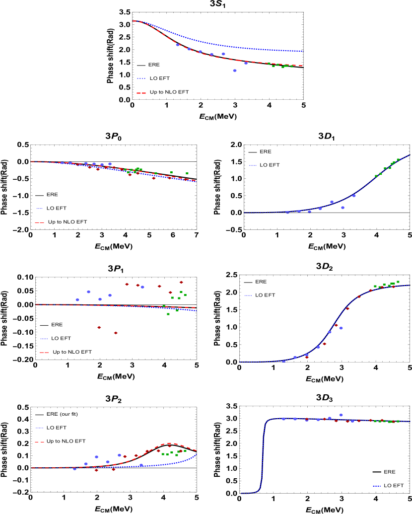
Figure 3: Comparison of the ERE and our two-body cluster EFT fits for the $d-\alpha$ scattering phase shift. The blue-dotted, red-dashed and black solid lines represent LO EFT, up-to-NLO EFT and ERE results, respectively. Circles gruebler1975phase , squares A. Jenny , and diamonds schmelzbach1972phase are the experimental data. According to the described scheme in the Sec. II, we consider the influences of all three scattering length, effective range, and shape parameters of the $D$-wave channels simultaneously, so we have only single LO plot for the $D$ waves.

Table 1: The determined effective range parameters. The parameters were obtained from matching the LO (up-to-NLO) EFT and ERE relations to the available low-energy experimental data in Refs.A. Jenny ; schmelzbach1972phase ; gruebler1975phase for each channel $\xi=$${}^{3}\!S_{1}$, ${}^{3}\!P_{0}$, ${}^{3}\!P_{1}$, ${}^{3}\!P_{2}$, ${}^{3}\!D_{1}$, ${}^{3}\!D_{2}$, and ${}^{3}\!D_{3}$ as shown in Fig. 3. The last column shows the deviations of fits from phase shifts experimental data.

$\xi$	Method	$\small{a^{[\xi]}[{\textrm{MeV}^{-2l-1}}]}$	$\small{r^{[\xi]}[{\textrm{MeV}^{2l-1}}]}$	$\small{s^{[\xi]}[{\textrm{MeV}^{2l-3}}]}$	${\chi^{[\xi]}}^{2}$
	LO EFT	$\small{-2.060\times 10^{-2}}$	$\,\,\,\,\,\,\,\,3.533\times 10^{-3}$	$-$	$2.6187$
${}^{3}\!S_{1}$	NLO EFT	$-2.780\times 10^{-2}$	$\,\,\,\,\,\,\,\,3.830\times 10^{-3}$	$-8.345\times 10^{-7}$	$0.0775$
	ERE	$-2.757\times 10^{-2}$	$\,\,\,\,\,\,\,\,3.137\times 10^{-3}$	$-7.688\times 10^{-7}$	$0.0283$
	LO EFT	$-8.029\times 10^{-7}$	$\,\,\,\,\,2.163\times 10^{2}$	$-$	$0.0069$
${}^{3}\!P_{0}$	NLO EFT	$-7.824\times 10^{-7}$	$\,\,\,\,\,1.356\times 10^{2}$	$\,\,\,\,\,1.950\times 10^{-3}$	$0.0014$
	ERE	$-4.364\times 10^{-7}$	$\,\,\,\,\,1.496\times 10^{2}$	$\,\,\,\,\,1.634\times 10^{-3}$	$0.0001$
	LO EFT	$-2.161\times 10^{-8}$	$-6.166\times 10^{3}$	$-$	$0.0433$
${}^{3}\!P_{1}$	NLO EFT	$-1.004\times 10^{-8}$	$-7.494\times 10^{3}$	$\!\!\!\!\!\!\!\!\!\!\!\!\!\!0.474$	$0.0024$
	ERE	$-1.012\times 10^{-8}$	$-8.494\times 10^{3}$	$\!\!\!\!\!\!\!\!\!\!\!\!\!\!0.452$	$0.0021$
	LO EFT	$\,\,\,\,\,1.297\times 10^{-8}$	$\,\,\,\,\,1.124\times 10^{5}$	$-$	$1.4657$
${}^{3}\!P_{2}$	NLO EFT	$\,\,\,\,\,2.014\times 10^{-8}$	$\,\,\,\,\,1.874\times 10^{5}$	$\!\!\!\!\!\!\!\!\!\!\!\!\!\!\!\!\!\!-1.851$	$1.8406$
	ERE	$\,\,\,\,\,2.037\times 10^{-8}$	$\,\,\,\,\,1.864\times 10^{5}$	$\!\!\!\!\!\!\!\!\!\!\!\!\!\!\!\!\!\!-1.865$	$1.5520$
${}^{3}\!D_{1}$	LO EFT/ERE	$\,\,-1.375\times 10^{-10}$	$\,\,\,\,\,1.012\times 10^{6}$	$\!\!-1.905\times 10^{3}$	$0.5597$
${}^{3}\!D_{2}$	LO EFT/ERE	$\,\,-1.716\times 10^{-10}$	$-7.086\times 10^{5}$	$\!\!\!\!\!\!\!\!\!\!\!\!\!\!\!\!\!\!-10.958$	$0.0033$
${}^{3}\!D_{3}$	LO EFT/ERE	$-4.500\times 10^{-8}$	$-1.554\times 10^{6}$	$1.303\times 10^{3}$	$0.0028$

The determined effective range parameters of channel $\xi$ has been reported in Table 1. The quality of description of available results $f^{ave}$ on the basis of the certain expression $f$ can be estimated by the $\chi^{2}$ method which is written as MMA-dt-dt

$${}\chi^{2}=\frac{1}{N}\sum^{N}_{i=1}\Big{[}\frac{f_{i}-f^{ave}}{f^{ave}}\Big{]}^{2},$$ (47)

where $N$ is the number of measurements. Taking into consideration $f$ as $\delta^{[\xi]}$ introduced in Eq. (46), the deviations of fits from used phase shift data for $\xi$ channel are obtained as shown in the last column of Table 1.

The phase shift analysis in Fig. 3 leads to the effective-range parameters presented in Table 1. Based on determined values from ERE fits, we propose a power-counting (PC) in which the effective-range parameters of $\xi$ channel are scaled as presented in Table 2. So, we can conclude that the main contribution of the scattering amplitude in all channels ${}^{3}\!S_{1}$, ${}^{3}\!P_{0}$, ${}^{3}\!P_{1}$, ${}^{3}\!P_{2}$, ${}^{3}\!D_{1}$ and ${}^{3}\!D_{2}$ come clearly from their scattering lengths, and the influences of both their effective ranges and shape parameters are small and can be considered as higher-order corrections. In this analysis, the effective-range and shape-parameter terms are suppressed by $(Q/\mathrm{\Lambda})^{n}$ and $(Q/\mathrm{\Lambda})^{m}$ as compared to the leading term of the ${}^{3}\!S_{1}$, ${}^{3}\!P_{0}$, ${}^{3}\!P_{1}$, ${}^{3}\!P_{2}$, ${}^{3}\!D_{1}$ and ${}^{3}\!D_{2}$ with $n=3,~{}3,~{}2,~{}1,~{}2,~{}3$ and $m=5,~{}7,~{}5,~{}4,~{}3,~{}5$, respectively.

For the ${}^{3}\!D_{3}$ partial wave, it seems that the contribution of both scattering length and shape parameters in comparison with the effective range term are one order down. However, no missing any physical effect, we would consider $-\frac{1}{a}+\frac{1}{2}rp^{2}+\frac{1}{4}sp^{4}\sim Q^{2}\mathrm{\Lambda}^{3}$ in the leading order. Furthermore, in the case corresponds to the large value of $\eta_{p}$, the term $H_{l}(\eta_{p})$ is significantly different from the usual unitary term $ip$. Therefore, in this case, the unitary term leads to $H(\eta_{p})\!\sim\!p^{2}/12k_{C}^{2}$ Higa-Hammer . For the $S$-wave channels, $H_{0}(\eta_{p})$ is comparable in magnitude to the effective-range term and can be automatically captured by taking $3k_{C}\sim\mathrm{\Lambda}$. Alternatively, one can enhance by a factor of $\mathrm{\Lambda}/Q$ the size of the ${}^{3}S_{1}$ effective range. In the $P$ waves, we have $H_{1}(\eta_{p})\!\sim\!Q^{3}(1\!+\!Q/\mathrm{\Lambda})$ and the term including $H(\eta_{p})$ can be also managed by redefining the effective range and shape parameter MMA-dt-dt . Scaling $\frac{1}{24}k_{C}^{3}\!\sim\!Q^{3}$, $\frac{5}{24}k_{C}\!\sim\!Q$ and $6k_{C}\!\sim\!\mathrm{\Lambda}$, the function $H_{l}(\eta_{p})$ can be estimated for the $l\!=\!2$ partial waves as $H_{2}(\eta_{p})\sim Q^{5}(1+1+Q/\mathrm{\Lambda})$. So, for the $D$ waves, the functions of $p^{2}$ and $p^{4}$ can be captured by the effective range and shape parameter, respectively, and the term regarding the $p^{6}$ would be negligible in the current theory.

Table 2: The suggested power-counting for the effective range parameters. $Q$ and $\mathrm{\Lambda}$ denote the low- and high-momentum scales as introduced in the text.

$[\xi]$	$1/a^{[\xi]}$	$r^{[\xi]}/2$	$s^{[\xi]}/4$
${}^{3}\!S_{1}$	${\mathrm{\Lambda}}$	${Q}/{\mathrm{\Lambda}^{2}}$	${Q}/{\mathrm{\Lambda}^{4}}$
${}^{3}\!P_{0}$	${\mathrm{\Lambda}^{4}}/Q$	$\mathrm{\Lambda}$	${Q^{2}}/{\mathrm{\Lambda}^{3}}$
${}^{3}\!P_{1}$	$\mathrm{\Lambda}^{5}/Q^{2}$	${\mathrm{\Lambda}^{3}}/{Q^{2}}$	${1}/{Q}$
${}^{3}\!P_{2}$	$\mathrm{\Lambda}^{5}/Q^{2}$	${\mathrm{\Lambda}^{4}}/{Q^{3}}$	${\mathrm{\Lambda}}/{Q^{2}}$
${}^{3}\!D_{1}$	$\mathrm{\Lambda}^{5}$	$\mathrm{\Lambda}^{3}$	${\mathrm{\Lambda}^{2}}/{Q}$
${}^{3}\!D_{2}$	$\mathrm{\Lambda}^{5}$	$Q\mathrm{\Lambda}^{2}$	$Q$
${}^{3}\!D_{3}$	$Q^{3}\mathrm{\Lambda}^{2}$	$\mathrm{\Lambda}^{3}$	${\mathrm{\Lambda}^{2}}/{Q}$

Taking into consideration the LO and NLO values of effective range parameters corresponding to the scheme used in Table 1, the LO and NLO values of EFT LECs for channel $\xi$ are determined as indicated in the first and second rows of Table 3. Based on the suggested PC in Table 2, the estimation of the LECs for each channel are presented as ”PC estimation” in Table 3. The orders of obtained EFT LECs are meaningfully consistent with the predictions of the suggested PC.

IV Differential Cross Section

In this section, we present the obtained results of the $d-\alpha$ differential cross section in the two-body cluster EFT approach. The differential cross section for the $d-\alpha$ elastic scattering with the contributions of the Coulomb and the strong interactions is given by

$$\frac{d\sigma}{d\Omega}=\Big{(}\frac{\mu}{2\pi}\Big{)}^{2}|T_{C}+T_{CS}|^{2}.$$ (48)

Table 3: The obtained EFT coupling constants for all $l=0,~{}1,~{}2$ channels using the determined effective-range parameters in Table 1. The LO and NLO results are consistent with the suggested scheme as introduced in the Sec. II. The last row in each channel states our suggested PC estimation based on Table 2.

$\xi$	Order	$\quad\small{\mathrm{\Delta}_{\!R}^{[\xi]}}[\textrm{MeV}]$	$\small{g_{\!R}^{[\xi]}}[\textrm{MeV}^{-(2l+1)/2}]$	$\small{h_{\!R}^{[\xi]}}[\textrm{MeV}^{-1}]$
	LO	$\!\!-10.944$	$3.360\times 10^{-2}$	$-$
${}^{3}\!S_{1}$	NLO	$-7.467$	$3.231\times 10^{-3}$	$0.272$
	PC estimation	​​​​​​​​​​​​​​$\frac{\mathrm{\Lambda}^{3}}{2\mu Q}\!=\!16.175$	​​​​​​​​​$(\frac{\pi\mathrm{\Lambda}^{2}}{\mu^{2}Q})^{\frac{1}{2}}\!=3.003\times 10^{-2}$	​​​​​​​​​$\frac{2\mu}{\mathrm{\Lambda}^{2}}\!=0.309$
	LO	$-4.577$	$2.352\times 10^{-4}$	​​​​​$-$
${}^{3}\!P_{0}$	NLO	$\!\!-13.091$	$2.977\times 10^{-4}$	$\qquad\quad\,-1.801\times 10^{-2}$
	PC estimation	​​​​​​​​​​​​​​$\frac{\mathrm{\Lambda}^{3}}{2\mu Q}\!=\!16.175$	​​​​​​​​$(\frac{3\pi}{\mu^{2}\mathrm{\Lambda}})^{\frac{1}{2}}\!=2.584\times 10^{-4}$	​​​​​​​​$\frac{2\mu Q^{2}}{\mathrm{\Lambda}^{4}}\!=1.236\times 10^{-2}$
	LO	$\,\,\,\,5.992$	$4.416\times 10^{-5}$	$-$
${}^{3}\!P_{1}$	NLO	$\,\,10.607$	$4.006\times 10^{-5}$	$\qquad\quad\,\,\,\,7.930\times 10^{-2}$
	PC estimation	​​​​​​​​​​​$\frac{\mathrm{\Lambda}^{2}}{2\mu}\!=\!\,\,\,3.235$	​​​​​​​​​​$(\frac{3\pi Q^{2}}{\mu^{2}\mathrm{\Lambda}^{3}})^{\frac{1}{2}}\!=5.169\times 10^{-5}$	​​​​​​​$\frac{2\mu Q}{\mathrm{\Lambda}^{3}}\!=6.182\times 10^{-2}$
	LO	$\,\,\,\,\,5.474$	$3.269\times 10^{-5}$	$-$
${}^{3}\!P_{2}$	NLO	2.114	$2.532\times 10^{-5}$	$\,\,0.123$
	PC estimation	​​​​​​​​​​​​$\frac{Q\mathrm{\Lambda}}{2\mu}\!=\!\,\,\,0.647$	​​​​​​​​​​$(\frac{3\pi Q^{3}}{\mu^{2}\mathrm{\Lambda}^{4}})^{\frac{1}{2}}\!=2.312\times 10^{-5}$	​​​​​​​​​​​​​​​$\frac{2\mu Q}{\mathrm{\Lambda}^{3}}\!=0.062$
${}^{3}\!D_{1}$	LO	$-5.730$	$4.448\times 10^{-6}$	$\,\,\,\,\!\!\,0.235$
	PC estimation	​​​​​​​​​​​​​$\frac{\mathrm{\Lambda}^{2}}{2\mu}\!=\,\,3.235$	​​​​​​​​​$(\frac{5\pi}{\mu^{2}\mathrm{\Lambda}^{3}})^{\frac{1}{2}}\!=3.707\times 10^{-6}$	​​​​​​​​​​​​​$\frac{2\mu}{\mathrm{\Lambda}Q}\!=1.545$
${}^{3}\!D_{2}$	LO	$\,\,\,\,\,6.568$	$5.318\times 10^{-6}$	​​​​​    ​​ $-0.017$
	PC estimation	​​​​​​​​​​​​​​$\frac{\mathrm{\Lambda}^{3}}{2\mu Q}\!=\!16.175$	​​​​​​​​​​​​$(\frac{5\pi}{\mu^{2}\mathrm{\Lambda}^{2}Q})^{\frac{1}{2}}\!=\!8.291\times 10^{-6}$	​​​​​​​​​​​​​$\frac{2\mu}{\mathrm{\Lambda}^{2}}\!=0.309$
${}^{3}\!D_{3}$	LO	$\quad\quad\quad\quad 1.578\times 10^{-2}$	$1.888\times 10^{-6}$	$1.450$
	PC estimation	​​​​​​​​​​​​​$\frac{Q^{3}}{2\mu\mathrm{\Lambda}}\!=\!\!\,\,\,2.588\times 10^{-2}$	​​​​​​​​​$(\frac{5\pi}{\mu^{2}\mathrm{\Lambda}^{3}})^{\frac{1}{2}}\!=\!3.707\times 10^{-6}$	​​​​​​​​​​​​​​$\frac{2\mu}{\mathrm{\Lambda}Q}\!=\!1.545$

Taking into account the determined values of EFT LECs presented in Table 3, we can compute the differential cross section at different CM energies and scattering angles. In order to calculate the differential cross section for the low-energy $d-\alpha$ elastic scattering, some important issues should be clarified. At the low energies, the cross section gets the dominant contribution from the leading term of the scattering amplitude in the ³$\!S_{1}$ partial wave. Thus, regarding the phase shift analysis for all $S$-, $P$- and $D$-wave channels in Tables 1 and 2, the leading $d-\alpha$ scattering cross section constructed by the relation corresponding to the scattering length of ³$\!S_{1}$ channel.

Based on our analysis in the previous section, the biggest corrections on the LO cross section comes from the effective range of ³$\!S_{1}$ and also the scattering length and effective range of ³$\!D_{3}$ partial wave corresponding to the first four terms of Lagrangian (17). These corrections are two orders down with respect to the effect of the ³$\!S_{1}$ scattering length. Remained effective range parameters could be neglected as $\textrm{N}^{3}\textrm{LO}$ and higher-order contributions in the current calculation.

Our results for the differential cross section versus the CM scattering angle for the $d-\alpha$ scattering are shown in Fig. 4 for the laboratory energies $E_{Lab}=0.87$, 2.15, 2.46, and 2.94 MeV. The contribution of $S$-, $P$- and $D$- waves in the differential cross section are shown in the first column of Fig. 4. And also, the results of the cross section with the ³$\!S_{1}$ (³$\!S_{1}$ and ³$\!D_{3}$) partial wave(s) are depicted by the dashed (solid) line in the second column of Fig. 4. The symbols in Fig. 4 indicate the reported experimental data from Refs. ohlsen1964deuteron ; blair1949scattering .

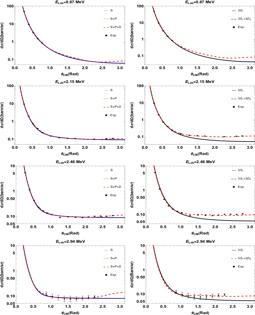
Figure 4: Differential cross sections for the low-energy $d-\alpha$ elastic scattering against the CM angle. Our EFT results are plotted with the laboratory energies $E_{Lab}=0.87$, 2.15, 2.46, and 2.94 MeV. The left column shows the the calculated EFT cross section with the contribution of the $S$ (black-solid), $S$+$P$ (blue-dotted) and $S$+$P$+$D$ (red-dashed). The right column indicate our plots for the differential cross section using the leading terms of ${}^{3}\!S_{1}$ only (black-solid), and the leading scattering terms in ${}^{3}\!S_{1}$ including the effects of ${}^{3}\!D_{3}$ channel (red-dashed). The dots are the experimental data from Refs. ohlsen1964deuteron ; blair1949scattering .

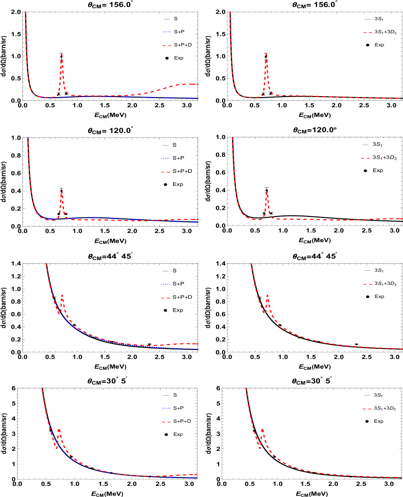
Figure 5: Differential cross sections for the low-energy $d-\alpha$ elastic scattering against the CM energy. Our EFT results are plotted with scattering angle $\theta_{CM}\!=\!156^{\circ}$, $120^{\circ}$, $44^{\circ}{45}^{\prime}$ and $30^{\circ}5^{\prime}$. All notations are as in Fig. 4

We have also plotted the differential cross sections of the $d-\alpha$ elastic scattering against CM energy with scattering angle $\theta_{CM}\!=\!156^{\circ}$, $120^{\circ}$, $44^{\circ}{45}^{\prime}$ and $30^{\circ}5^{\prime}$ in Fig. 5. Our EFT results using the ³$\!S_{1}$ (³$\!S_{1}$ and ³$\!D_{3}$) channel(s) are depicted by the dashed (solid) line, and the circles in Fig. 5 indicate the experimental data in Ref. ohlsen1964deuteron ; blair1949scattering . Fig. 5 shows that in our EFT formalism the peak manner of the differential cross section around $E_{CM}\sim 0.706$ MeV can be reproduced only by including the ³$\!D_{3}$ scattering amplitude with the influences regarding its scattering length and effective range. It seems that the contributions of the ³$\!D_{3}$ would be more important and it must be included in our EFT calculations to reproduce reliably the low-energy experimental data.

Our EFT results in Figs. 4 and 5 indicate that the ³$\!S_{1}$ and ³$\!D_{3}$ scattering amplitudes could reproduce the low-energy experimental data and other partial waves have no significant effect at the current low-energy regime as we expected from the suggested PC.

V Conclusion

In this paper, we have studied the low-energy $d-\alpha$ elastic scattering using two-body cluster EFT approach. Our constructed cluster EFT treats the deuteron and alpha nucleus as the point-like nuclear clusters, so we have concentrated on the energy region $E_{CM}\lesssim 3.3$ MeV. At the present energy region, the Coulomb force has been considered as a non-perturbative treatment. Here, we have studied all possible $S$-, $P$- and $D$-wave channels. We have introduced a scheme in which the LO contributions of phase shift in each partial wave of $l=0,1$ channels has been constructed from its scattering length and effective range and its shape parameter influence has been included at the NLO order. Also, the additional 2nd-order kinetic term with constant $h^{[\xi]}$ is needed to renormalize the interacting $D$-wave propagator which contains up to quintic divergences.

Using the available low-energy phase shift data, we obtained the values of the effective range parameters $S$, $P$ and $D$ waves. The EFT LECs for $l=0,1,2$ partial waves evaluated in terms of effective range parameters. Our ERE fitted curves and the cluster EFT calculations for the $S$-, $P$- and $D$-wave phase shifts have good consistency with the available results and a converging pattern from LO to NLO. We have plotted the differential cross sections against the CM scattering angle and also the CM energy. The comparison our obtained two-body cluster EFT results to the experimental data indicates good consistency.

Our obtained EFT results indicate that the cross section of the $d-\alpha$ scattering got the dominant contributions using the scattering amplitude of ³$\!S_{1}$ partial wave containing the dimeron propagator without kinetic energy terms. It regards the ³$\!S_{1}$ scattering-length effect as we expected from our PC analysis. We have also showed that the resonance behavior of the $d-\alpha$ cross section can be reproduced only by including the contribution of the ³$\!D_{3}$ scattering amplitude. It is consistent to our PC estimation in which the largest corrections on the leading $d-\alpha$ scattering cross section are constructed by the strong interacting contributions corresponding to the ³$\!S_{1}$ effective range and also ³$\!D_{3}$ scattering length and effective range. It should be mentioned that other strong interacting terms can be omitted because of small contributions of orders $\textrm{N}^{3}\textrm{LO}$ and higher in the total low-energy cross section.

The discrepancy of our results for the cross section above $E_{CM}>3.3$ MeV can be handled by introducing the three-body cluster EFT in which neutron, proton and alpha particle are the degrees of freedom. In the present EFT calculation based on considering the deuteron as a point-like particle, the EFT results for $E_{CM}>3.3$ MeV are questionable and we should switch to the three-body cluster formalism for the higher energies.

It would be interesting to use our results for studying of the $d+\alpha$ $\rightarrow^{6}$$\textrm{Li}+\gamma$ astrophysical radiative capture based on halo/cluster EFT calculation in the future. The $d-\alpha$ scattering and radiative capture can also be studied by the three-body EFT formalism for the higher-energy region.

Appendix A Derivation of the elastic scattering amplitudes

In this section, we present the detailed derivation of the $d-\alpha$ elastic scattering amplitudes for all possible partial waves, $l=0,~{}1,~{}2$.

$S-$wave channel

According to the Lagrangian (17), the strong interaction in the $\xi={{}^{3}\!S_{1}}$ channel of the $d-\alpha$ system can be described using the up-to-NLO Lagrangian

$${}\mathcal{L}^{[\xi]} = \phi^{\dagger}(i\partial_{0}+\frac{\nabla^{2}}{2m_{\alpha}})\phi+d_{i}^{\dagger}(i\partial_{0}+\frac{\nabla^{2}}{2m_{d}})d_{i}$$ (49)

$$+\,\eta^{[\xi]}\bar{t}_{i}^{\,\dagger}\Big{[}i\partial_{0}\!+\!\frac{\nabla^{2}}{2m_{t}}\!-\!\mathrm{\Delta}^{[\xi]}\Big{]}\bar{t}_{i}+h^{[\xi]}\bar{t}_{i}^{\,\dagger}\Big{[}i\partial_{0}+\frac{\nabla^{2}}{2m_{t}}\Big{]}^{2}\bar{t}_{i}$$

$$+\,g^{[\xi]}\Big{[}\bar{t}^{\,\dagger}_{i}(\phi\,d_{i})\!+\!h.c.\Big{]},$$

where $\bar{t}_{i}$ is the vector auxiliary field of the ${{}^{3}\!S_{1}}$ dimeron. According to the Feynman diagram of Fig. 2, the up-to-NLO EFT scattering amplitude in the ${}^{3}\!S_{1}$ channel can be written as

$${}-iT_{CS}^{[\xi]}e^{2i\sigma_{0}} = (-ig^{[\xi]})^{2}\,\chi_{p^{\prime}}^{*(-)}(\mathbf{0})\,\varepsilon_{j}^{d*}\,\varepsilon_{j}^{\bar{t}}\,iD^{[\xi]}(E,\textbf{0})\varepsilon_{i}^{\bar{t}*}\,\varepsilon_{i}^{d}\,\chi_{p}^{(+)}(\mathbf{0})$$ (50)

$$= -ig^{[^{3}S_{1}]^{2}}D^{[n,^{3}S_{1}]}(E,\textbf{0})\,\varepsilon_{j}^{d*}\,\varepsilon_{j}^{t}\,\varepsilon_{i}^{t*}\,\varepsilon_{i}^{d}\,\chi_{p^{\prime}}^{*(-)}(\mathbf{0})\chi_{p}^{(+)}(\mathbf{0})$$

$$= -ig^{[\xi]^{2}}\!D^{[\xi]}(E,\textbf{0})W_{0}(\eta_{p})C_{0}^{2}(\eta_{p})e^{2i\sigma_{0}},$$

where $\varepsilon_{i}^{d}$ and $\varepsilon_{i}^{\bar{t}}$ are polarization vectors of the deuteron and dimeron auxiliary fields respectively, which satisfy the relations

$${}\varepsilon_{j}^{\bar{t}*}\,\varepsilon_{i}^{\bar{t}}=\delta_{ij},\quad\quad\varepsilon_{j}^{d*}\,\varepsilon_{i}^{d}=\frac{1}{3}\delta_{ij}.$$ (51)

In the last equality of Eq. (50) we use

$${}\chi_{p^{\prime}}^{*(-)}(\mathbf{0})\chi_{p}^{(+)}(\mathbf{0})=W_{0}(\eta_{p})\,C_{0}^{2}(\eta_{p})e^{2i\sigma_{0}}.$$ (52)

According to the diagrams in second line of Fig. 2, The $S$-wave up-to-NLO full propagator is given by

$${}D^{[\xi]}(E,\textbf{0}) = \frac{\eta^{[\xi]}}{E-\mathrm{\Delta}^{[\xi]}-\eta^{[\xi]}g^{[\xi]^{2}}J_{0}(E)}\Big{[}\underbrace{\,1}_{\mathrm{LO}}-\underbrace{\frac{\eta^{[\xi]}h^{[\xi]}E^{2}}{E-\mathrm{\Delta}^{[\xi]}-\eta^{[\xi]}g^{[\xi]^{2}}J_{0}(E)}}_{\mathrm{NLO}~{}\mathrm{corection}}\Big{]},\quad\quad\quad$$ (53)

where the fully dressed bubble $J_{0}$, which is described the propagation of the particles from initially zero separation and back to zero separation, is written as

$${}J_{0}(E) = \lim_{\mathbf{r}^{\prime},\mathbf{r}\rightarrow\mathbf{0}}\langle\mathbf{r}^{\prime}|G_{C}^{(+)}{(E)}|\mathbf{r}\rangle$$ (54)

$$= 2\mu\int\frac{d^{3}q}{(2\pi)^{3}}\frac{\chi_{q}^{(+)}(\mathbf{0})\chi_{q}^{*(+)}(\mathbf{0})}{2\mu E-q^{2}+i\epsilon}$$

$$= 2\mu\!\int\!\frac{d^{3}q}{(2\pi)^{3}}\frac{2\pi\eta_{q}}{e^{2\pi\eta(q)}-1}\,\frac{1}{p^{2}-q^{2}+i\epsilon}$$

$$= \underbrace{2\mu\!\int\!\frac{d^{3}q}{(2\pi)^{3}}\frac{2\pi\eta_{q}}{e^{2\pi\eta_{q}}-1}\,\frac{1}{q^{2}}\frac{p^{2}}{p^{2}-q^{2}+i\epsilon}}_{J^{fin}_{0}}$$

$$\underbrace{-2\mu\!\int\!\frac{d^{3}q}{(2\pi)^{3}}\frac{2\pi\eta_{q}}{e^{2\pi\eta_{q}}-1}\,\frac{1}{q^{2}}}_{J^{div}_{0}}.\qquad\qquad$$

Calculation of the finite part of the $S$-wave Coulomb bubble leads to 33

$${}J^{fin}_{0}=-\frac{\mu}{\pi}k_{C}W_{0}(\eta_{p})H(\eta_{p})=-\frac{\mu}{2\pi}H_{0}(\eta_{p}),$$ (55)

and taking into account the power divergence subtraction (PDS) regularization scheme, the momentum independent divergent part is obtained as 33

$$J^{div}_{0}\!=\!-\frac{\mu}{2\pi}\bigg{\{}\!\frac{\kappa}{D-3}\!+\!2k_{C}\!\bigg{[}\!\frac{1}{D-4}\!-\!\textrm{ln}\big{(}\frac{\kappa\sqrt{\pi}}{2k_{C}}\big{)}\!-\!1\!+\!\frac{3}{2}C_{E}\!\bigg{]}\!\bigg{\}},$$

with $D$ the dimensionality of spacetime, $\kappa$ the renormalization mass scale and $C_{E}$ Euler-Masheroni constant. Instead of PDS regularization scheme we can use a simple momentum cutoff $\mathrm{\Lambda}$ to make the divergent integral $J^{div}_{0}$ finite. It then becomes 33

$$J^{div}_{0} \!=\! -\frac{2\mu}{\pi}\!\int_{0}^{\mathrm{\Lambda}}\!dq\frac{\eta_{q}}{e^{2\pi\eta_{q}}-1}$$

$$\!=\! -\frac{2\mu k_{C}}{\pi}\!\int_{\frac{2\pi k_{C}}{\mathrm{\Lambda}}}^{\infty}\,\!\frac{dx}{x(e^{x}-1)}$$

$$\!=\! -\frac{2\mu k_{C}}{\pi}\Bigg{\{}\!\int_{0}^{\infty}\!\frac{dx}{x(e^{x}-1)}\!-\!\int_{0}^{\frac{2\pi k_{C}}{\mathrm{\Lambda}}}\frac{dx}{x(e^{x}-1)}\Bigg{\}}\!$$

$$\!=\! -\frac{2\mu k_{C}}{\pi}\Bigg{\{}\!\mathrm{\Gamma}(0)\zeta(0)\!-\!\int_{0}^{\frac{2\pi k_{C}}{\mathrm{\Lambda}}}\!\!dx\bigg{(}\!\frac{1}{x^{2}}-\frac{1}{2x}+\mathcal{O}\,(x^{0})\!\bigg{)}\!\!\Bigg{\}}\!$$

$$\!=\! -\frac{2\mu k_{C}}{\pi}\Big{(}\frac{1}{2}C_{E}+\frac{\mathrm{\Lambda}}{2\pi k_{C}}-\frac{1}{2}\ln\frac{\mathrm{\Lambda}}{k_{C}}+\mathcal{O}\,(\frac{2\pi k_{C}}{\mathrm{\Lambda}})\!\Big{)},$$

where in the second line we use changing integral variable $x=2\pi\eta_{q}$, and in the last line we use

$$\mathrm{\Gamma}(0) = \lim_{\epsilon\rightarrow 0}\big{(}\frac{1}{\epsilon}-C_{E}\big{)},$$ (58)

$$\zeta(0) = \lim_{\epsilon\rightarrow 0}\Big{(}-\frac{1}{2}(1+\epsilon\ln 2\pi)+\mathcal{O}\,(\epsilon^{2})\Big{)}.$$ (59)

Thus, the up-to-NLO EFT scattering amplitude of Eq. (50) is rewritten

$$\!\!T^{[\xi]}_{CS}\! = \!-\frac{2\pi}{\mu}\frac{C_{0}^{2}(\eta_{p})W_{0}(\eta_{p})}{(\frac{2\pi\mathrm{\Delta}^{[\xi]}}{\eta^{[\xi]}g^{[\xi]^{2}}\!\mu}\!+\!\frac{2\pi}{\mu}J^{div}_{0})\!-\!\frac{1}{2}(\frac{2\pi}{\eta^{[\xi]}g^{[\xi]^{2}}\!\mu^{2}})p^{2}\!-\!H_{0}(\eta_{p})}$$

$$\times\Big{[}\underbrace{\,1}_{\mathrm{\!\!LO}}\!\!\!\!+\!\underbrace{\frac{1}{4}\frac{(\frac{2\pi h^{[\xi]}}{g^{[\xi]^{2}}\!\mu^{3}})}{(\frac{2\pi\mathrm{\Delta}^{[\xi]}}{\eta^{[\xi]}g^{[\xi]^{2}}\mu}\!+\!\frac{2\pi}{\mu}J^{div}_{0})\!-\!\frac{1}{2}(\frac{2\pi}{\eta^{[\xi]}g^{[\xi]^{2}}\!\mu^{2}})p^{2}\!-\!H_{0}(\eta_{p})}p^{4}\,\,}_{\mathrm{NLO}~{}\mathrm{corection}}\!\!\Big{]}\!.$$

Regardless of which renormalization scheme we use to calculate the divergent integral $J^{div}_{0}$, this momentum independent divergence part is absorbed by the parameter $\mathrm{\Delta}^{[\xi]}$ via introducing the renormalized parameter $\mathrm{\Delta}^{[\xi]}_{R}$ as Higa-Hammer

$$\mathrm{\Delta}^{[\xi]}_{R}=\mathrm{\Delta}^{[\xi]}+\eta^{[\xi]}g^{[\xi]^{2}}J^{div}_{0}.$$ (61)

Finally, the up-to-NLO scattering amplitude for $\xi\!=\!{{}^{3}\!S_{1}}$ partial wave is expressed as

$$T^{[\xi]}_{CS} = \frac{2\pi}{\mu}\frac{C_{0}^{2}(\eta_{p})W_{0}(\eta_{p})}{\frac{2\pi\mathrm{\Delta}_{R}^{[\xi]}}{\eta^{[\xi]}g^{[\xi]^{2}}\!\mu}-\frac{1}{2}(\frac{2\pi}{\eta^{[\xi]}g^{[\xi]^{2}}\!\mu^{2}})p^{2}\!-\!H_{0}(\eta_{p})}$$

$$\times\Big{[}\underbrace{\,\,1}_{\mathrm{LO}}+\!\underbrace{\frac{1}{4}\frac{(\frac{2\pi h^{[\xi]}}{g^{[\xi]^{2}}\!\mu^{3}})}{\frac{2\pi\mathrm{\Delta}_{R}^{[\xi]}}{\eta^{[\xi]}g^{[\xi]^{2}}\!\mu}-\frac{1}{2}(\frac{2\pi}{\eta^{[\xi]}g^{[\xi]^{2}}\!\mu^{2}})p^{2}\!-\!H_{0}(\eta_{p})}p^{4}\,\,}_{\mathrm{NLO}~{}\mathrm{corection}}\!\!\Big{]}.$$

$P-$wave channels

The up-to-NLO Lagrangian for the strong interaction in the $\xi=$${{}^{3}\!P_{0}}$ channel of the $d-\alpha$ system can be written as

$${}\mathcal{L}^{[\xi]} = \phi^{\dagger}(i\partial_{0}+\frac{\nabla^{2}}{2m_{\alpha}})\phi+d_{i}^{\dagger}(i\partial_{0}+\frac{\nabla^{2}}{2m_{d}})d_{i}$$ (63)

$$+\,\eta^{[{\xi}]}t^{\dagger}\Big{[}i\partial_{0}+\frac{\nabla^{2}}{2m_{t}}-\mathrm{\Delta}^{[{\xi}]}\Big{]}t+h^{[{\xi}]}t^{\dagger}\Big{[}i\partial_{0}+\frac{\nabla^{2}}{2m_{t}}\Big{]}^{2}t$$

$$+\sqrt{3}\,g^{[{\xi}]}\Big{[}t^{\dagger}(\phi\mathcal{P}_{i}d_{i})+h.c.\Big{]},$$

where $t$ is the scaler auxiliary field of the ${}^{3}\!P_{0}$ dimeron. According to the Feynman diagrams of Fig. 2 we have

$$-i3T^{[\xi]}_{CS}P_{1}(\hat{\textbf{p}}^{\prime}\cdot\hat{\textbf{p}})e^{2i\sigma_{1}} = 3(-ig^{[\xi]})^{2}[\mathcal{P}^{*}_{j}\chi_{p^{\prime}}^{*(-)}(\mathbf{0})]\varepsilon_{j}^{d*}iD^{[\xi]}(E,\textbf{0})\,\varepsilon_{i}^{d}\,[\mathcal{P}_{i}\chi_{p}^{(+)}(\mathbf{0})]$$ (64)

$$= -3ig^{[\xi]^{2}}D^{[\xi]}(E,\textbf{0})\varepsilon_{j}^{d*}\,\varepsilon_{i}^{d*}[\nabla_{j}\chi_{p^{\prime}}^{*(-)}(\mathbf{0})][\nabla_{i}\chi_{p}^{(+)}(\mathbf{0})]$$

$$= -ig^{[\xi]^{2}}D^{[\xi]}(E,\textbf{0})C_{0}^{2}(\eta_{p})W_{1}(\eta_{p})P_{1}(\hat{\textbf{p}}^{\prime}\cdot\hat{\textbf{p}})e^{2i\sigma_{1}},\quad\quad\quad$$

where in the last line, the following relation is used

$${}[\nabla_{i}\chi_{p^{\prime}}^{*(-)}(\mathbf{0})][\nabla_{i}\chi_{p}^{(+)}(\mathbf{0})] = C^{2}_{0}(\eta_{p})\,p^{\prime}_{i}p_{i}\,(1+\eta_{p}^{2})e^{2i\sigma_{1}}$$

$$= C^{2}_{0}(\eta_{p})\,W_{1}(\eta_{p})P_{1}(\hat{\textbf{p}}^{\prime}\cdot\hat{\textbf{p}})e^{2i\sigma_{1}}.$$

The up-to-NLO strong interaction Lagrangian in the $\xi=$${{}^{3}\!P_{1}}$ channel is introduced as

$${}\mathcal{L}^{[\xi]} = \phi^{\dagger}(i\partial_{0}+\frac{\nabla^{2}}{2m_{\alpha}})\phi+d_{i}^{\dagger}(i\partial_{0}+\frac{\nabla^{2}}{2m_{d}})d_{i}$$ (66)

$$+\,\eta^{[\xi]}t_{i}^{\dagger}\Big{[}i\partial_{0}+\frac{\nabla^{2}}{2m_{t}}-\mathrm{\Delta}^{[\xi]}\Big{]}t_{i}+h^{[\xi]}t_{i}^{\dagger}\Big{[}i\partial_{0}+\frac{\nabla^{2}}{2m_{t}}\Big{]}^{2}t_{i}$$

$$+\sqrt{\frac{3}{2}}\epsilon_{kji}\,g^{[\xi]}\Big{[}t_{k}^{\dagger}(\phi\mathcal{P}_{j}d_{i})+h.c.\Big{]},$$

where $t_{i}$ denotes the vector field of the ${}^{3}\!P_{1}$ dimeron. So, the scattering amplitude in the ${}^{3}\!P_{1}$ channel is written as

$${}-i3T^{[\xi]}_{CS}P_{1}(\hat{\textbf{p}}^{\prime}\cdot\hat{\textbf{p}})e^{2i\sigma_{1}} = \frac{3}{2}(-ig^{[\xi]})^{2}\,[\mathcal{P}^{*}_{m}\chi_{p^{\prime}}^{*(-)}(\mathbf{0})]\epsilon_{lmj}\varepsilon_{j}^{d*}\,\varepsilon^{t}_{l}iD^{[\xi]}(E,\textbf{0})\epsilon_{ksi}\varepsilon_{k}^{t*}\,\varepsilon_{i}^{d}\,[\mathcal{P}_{s}\chi_{p}^{(+)}(\mathbf{0})]$$ (67)

$$= -\frac{1}{2}\,ig^{[\xi]^{2}}\,D^{[\xi]}(E,\textbf{0})\,\epsilon_{kmi}\,\epsilon_{ksi}[\nabla_{m}\chi_{p^{\prime}}^{*(-)}(\mathbf{0})]\,[\nabla_{s}\chi_{p}^{(+)}(\mathbf{0})]$$

$$= -ig^{[\xi]^{2}}D^{[\xi]}(E,\textbf{0})C_{0}^{2}(\eta_{p})W_{1}(\eta_{p})P_{1}(\hat{\textbf{p}}^{\prime}\cdot\hat{\textbf{p}})e^{2i\sigma_{1}},\quad$$

with $\varepsilon_{i}^{t}$ as the polarization vector of the ${}^{3}\!P_{1}$ dimeron auxiliary field. Also, the strong interaction Lagrangian for the $d-\alpha$ system in the $\xi={{}^{3}\!P_{2}}$ channel can be written as

$${}\mathcal{L}^{[\xi]} = \phi^{\dagger}(i\partial_{0}+\frac{\nabla^{2}}{2m_{\alpha}})\phi+d_{i}^{\dagger}(i\partial_{0}+\frac{\nabla^{2}}{2m_{d}})d_{i}$$ (68)

$$+\,\eta^{[\xi]}t_{ij}^{\dagger}\!\Big{[}i\partial_{0}\!+\!\frac{\nabla^{2}}{2m_{t}}\!-\!\mathrm{\Delta}^{[\xi]}\!\Big{]}t_{ij}\!+\!h^{[\xi]}t_{ij}^{\dagger}\!\Big{[}i\partial_{0}+\frac{\nabla^{2}}{2m_{t}}\Big{]}^{2}\!t_{ij}$$

$$+\frac{3}{\sqrt{5}}g^{[\xi]}\Big{[}\!t_{ij}^{\dagger}(\phi\mathcal{P}_{j}d_{i})+h.c.\Big{]},$$

where $t_{ij}$ is the auxiliary tensor field of the ${}^{3}\!P_{2}$ dimeron. Therefore, the scattering amplitude in the ${}^{3}\!P_{2}$ channel is obtained as

$${}-3iT^{[\xi]}_{CS}P_{1}(\hat{\textbf{p}}^{\prime}\cdot\hat{\textbf{p}})e^{2i\sigma_{1}} = \frac{9}{5}(-ig^{[\xi]})^{2}\,[\mathcal{P}^{*}_{m}\chi_{p^{\prime}}^{*(-)}(\mathbf{0})]\varepsilon_{j}^{d*}\,\varepsilon_{jm}^{t}iD^{[\xi]}(E,\textbf{0})\varepsilon_{si}^{t*}\,\varepsilon_{i}^{d}\,[\mathcal{P}_{s}\chi_{p}^{(+)}(\mathbf{0})]$$ (69)

$$= -ig^{[\xi]^{2}}\!D^{[\xi]}(E,\textbf{0})C_{0}^{2}(\eta_{p})W_{1}(\eta_{p})P_{1}(\hat{\textbf{p}}^{\prime}\cdot\hat{\textbf{p}})e^{2i\sigma_{1}},\qquad\qquad$$

with $\varepsilon_{ij}$ as the polarization tensor of the ${}^{3}\!P_{2}$ dimeron auxiliary field which satisfies the expression

$${}\varepsilon_{jm}^{t}\,\varepsilon_{si}^{t*}=\frac{1}{2}(\delta_{js}\delta_{mi}+\delta_{ji}\delta_{ms}-\frac{2}{3}\delta_{jm}\delta_{si}).$$ (70)

The up-to-NLO full propagator for the ${}^{3}\!P_{0}$, ${}^{3}\!P_{1}$ and ${}^{3}\!P_{2}$ channels is given by

$${}D^{[\xi]}(E,\textbf{0}) = \frac{\eta^{[\xi]}}{E-\mathrm{\Delta}^{[\xi]}-\frac{1}{3}\eta^{[\xi]}g^{[\xi]^{2}}J_{1}(E)}\Big{[}\underbrace{1}_{\mathrm{LO}}-\underbrace{\frac{\eta^{[\xi]}h^{[\xi]}E^{2}}{E\!-\mathrm{\Delta}^{[\xi]}\!-\frac{1}{3}\eta^{[\xi]}g^{[\xi]^{2}}J_{1}(E)}}_{\mathrm{NLO~{}corection}}\!\Big{]}\!.\quad\quad\quad$$ (71)

The function $J_{1}(E)$ is given by

$$J_{1}(E) \!= 2\mu\!\!\int\!\!\frac{d^{3}q}{(2\pi)^{3}}\frac{[\nabla_{i}\chi_{{q}}^{(+)}(\mathbf{0})][\nabla_{i}\chi_{{q}}^{*(+)}(\mathbf{0})]}{2\mu E-{q}^{2}+i\epsilon}$$ (72)

$$= 2\mu\!\!\int\!\!\frac{d^{3}q}{(2\pi)^{3}}\frac{q^{2}+k_{C}^{2}}{p^{2}-{q}^{2}+i\epsilon}\,\frac{2\pi\eta_{q}}{e^{2\pi\eta_{q}}-1}$$

$$= 2\mu\!\!\int\!\!\frac{d^{3}q}{(2\pi)^{3}}\frac{q^{2}}{p^{2}-{q}^{2}+i\epsilon}\,\frac{2\pi\eta_{q}}{e^{2\pi\eta_{q}}-1}\!+\!k_{C}^{2}J_{0}(E)$$

$$= 2\mu\!\!\int\!\!\frac{d^{3}q}{(2\pi)^{3}}\frac{q^{2}-p^{2}}{p^{2}-{q}^{2}+i\epsilon}\,\frac{2\pi\eta_{q}}{e^{2\pi\eta_{q}}-1}\!+\!(p^{2}\!+\!k_{C}^{2})J_{0}(E)$$

$$= W_{1}(\eta_{p})J_{0}(E)\underbrace{-2\mu\int\frac{d^{3}q}{(2\pi)^{3}}\,\frac{2\pi\eta_{q}}{e^{2\pi\eta_{q}}-1}}_{J}.\qquad$$

In the second line of Eq. (72) we use

$$[\nabla_{i}\chi_{q}^{(+)}(\mathbf{0})][\nabla_{i}\chi_{q}^{*(+)}(\mathbf{0})]\!=\!C^{2}_{0}(\eta_{q})W_{1}(\eta_{q}).$$ (73)

The integral $J$ is divergent and independent of the external momentum $p$. According to the PDS regularization scheme it takes the form Higa-Hammer

$$J=-4\pi\mu k_{C}^{2}\Big{(}k_{C}\zeta^{\prime}(-2)+\frac{\kappa}{24}\Big{)},$$ (74)

where $\zeta^{\prime}$ is derivative of the Riemann zeta function and $\zeta^{\prime}(-2)\!\approx\!-0.0304$. If we use the cutoff regularization scheme the integral $J$ takes the form

$$J \!=\! -\frac{2\mu}{\pi}\!\int_{0}^{\mathrm{\Lambda}}\!dqq^{2}\frac{\eta_{q}}{e^{2\pi\eta_{q}}-1}$$ (75)

$$\!=\! -8\pi\mu k^{3}_{C}\!\int_{\frac{2\pi k_{C}}{\mathrm{\Lambda}}}^{\infty}\!\,\frac{dx}{x^{3}(e^{x}-1)}$$

$$\!=\! -8\pi\mu k^{3}_{C}\Bigg{\{}\!\int_{0}^{\infty}\!\frac{dx}{x^{3}(e^{x}-1)}-\int_{0}^{\frac{2\pi k_{C}}{\mathrm{\Lambda}}}\frac{dx}{x^{3}(e^{x}-1)}\Bigg{\}}\!$$

$$\!=\! -8\pi\mu k^{3}_{C}\Bigg{\{}\mathrm{\Gamma}(-2)\zeta(-2)-\int_{0}^{\frac{2\pi k_{C}}{\mathrm{\Lambda}}}\!\!dx\bigg{(}\!\frac{1}{x^{4}}-\frac{1}{2x^{3}}+\frac{1}{12x^{2}}+\mathcal{O}\,(x^{0})\!\bigg{)}\!\!\Bigg{\}}\!$$

$$\!=\! -8\pi\mu k^{3}_{C}\bigg{\{}2\pi^{2}C_{E}\,\zeta^{\prime}(-2)\!+\!\frac{1}{3}\Big{(}\frac{\mathrm{\Lambda}}{2\pi k_{C}}\Big{)}^{\!3}\!-\!\frac{1}{4}\Big{(}\frac{\mathrm{\Lambda}}{2\pi k_{C}}\Big{)}^{\!2}\!+\!\frac{1}{12}\Big{(}\frac{\mathrm{\Lambda}}{2\pi k_{C}}\Big{)}+\mathcal{O}(\frac{2\pi k_{C}}{\mathrm{\Lambda}})\!\bigg{\}}$$

where in the second line we use $x=2\pi\eta_{q}$. Thus, $J_{1}$ can be divided as $J_{1}\!=\!J_{1}^{fin}\!+\!J_{1}^{div}$ with

$$J^{fin}_{1} = W_{1}(\eta_{p})J^{fin}_{0}=-\frac{\mu}{2\pi}H_{1}(\eta_{p}),$$ (76)

$$J^{div}_{1} = W_{1}(\eta_{p})J^{div}_{0}+J=p^{2}J^{div}_{0}+(k_{C}^{2}J^{div}_{0}+J).\qquad\quad$$ (77)

Consequently, the up-to-NLO EFT scattering amplitude of Eqs. (64), (67) and (69) is rewritten as

$$T^{[\xi]}_{CS} = -\frac{2\pi}{\mu}\frac{C_{0}^{2}(\eta_{p})W_{1}(\eta_{p})}{(\frac{6\pi\mathrm{\Delta}^{[\xi]}}{\eta^{[\xi]}g^{[\xi]^{2}}\mu}\!+\!\frac{2\pi}{\mu}(k_{C}^{2}J^{div}_{0}+J))\!-\!\frac{1}{2}(\frac{6\pi}{\eta^{[\xi]}g^{[\xi]^{2}}\mu^{2}}+\frac{2\pi}{\mu}J^{div}_{0})p^{2}\!-\!H_{1}(\eta_{p})}$$ (78)

$$\!\!\!\!\times\Big{[}\underbrace{1}_{\mathrm{LO}}+\!\underbrace{\frac{1}{4}\frac{(\frac{6\pi h^{[\xi]}}{g^{[\xi]^{2}}\mu^{3}})}{(\frac{6\pi\mathrm{\Delta}^{[\xi]}}{\eta^{[\xi]}g^{[\xi]^{2}}\mu}\!+\!\frac{2\pi}{\mu}(k_{C}^{2}J^{div}_{0}+J))\!-\!\frac{1}{2}(\frac{6\pi}{\eta^{[\xi]}g^{[\xi]^{2}}\mu^{2}}+\frac{2\pi}{\mu}J^{div}_{0})p^{2}\!-\!H_{1}(\eta_{p})}p^{4}\,\,}_{\mathrm{NLO}~{}\mathrm{corection}}\!\!\!\Big{]}$$

​The function $J_{1}^{div}$ has two divergences, momentum independent and momentum-squared. Regardless of PDS or cutoff renormalization scheme are used to calculate the divergent integrals $J_{0}^{div}$ and $J$, these momentum independent and momentum-squared divergence parts are absorbed by the parameters $\mathrm{\Delta}^{[\xi]}$, $g^{[\xi]}$ and $h^{[\xi]}$ via introducing the renormalized parameters $\mathrm{\Delta}_{R}^{[\xi]}$, $g_{R}^{[\xi]}$ and $h_{R}^{[\xi]}$ as

$$\mathrm{\Delta}^{[\xi]}_{R} =\frac{\mathrm{\Delta}^{[\xi]}+\frac{1}{3}\eta^{[\xi]}g^{[\xi]^{2}}(k_{C}^{2}J^{div}_{0}+J)}{1+\frac{1}{3}\eta^{[\xi]}g^{[\xi]^{2}}\mu J^{div}_{0}},$$ (79)

$$\frac{1}{g_{R}^{[\xi]^{2}}} =\frac{1}{g^{[\xi]^{2}}}+\frac{1}{3}\eta^{[\xi]}\mu J^{div}_{0},$$ (80)

$$h_{R}^{[\xi]} =\frac{h^{[\xi]}}{1+\frac{1}{3}\eta^{[\xi]}g^{[\xi]^{2}}\mu J^{div}_{0}}.$$ (81)

Finally, the up-to-NLO Coulomb-subtracted EFT scattering amplitude for ${}^{3}\!P_{0}$, ${}^{3}\!P_{1}$ and ${}^{3}\!P_{2}$ channels are obtained

$${}T^{[\xi]}_{CS} = -\frac{2\pi}{\mu}\frac{C_{0}^{2}(\eta_{p})W_{1}(\eta_{p})}{\frac{6\pi\mathrm{\Delta}_{\!R}^{[\xi]}}{\eta^{[\xi]}g_{\!R}^{[\xi]^{2}}\mu}\!-\!\frac{1}{2}(\frac{6\pi}{\eta^{[\xi]}g_{\!R}^{[\xi]^{2}}\mu^{2}})p^{2}\!-\!H_{1}(\eta_{p})}\Big{[}\underbrace{\,\,1}_{\mathrm{LO}}+\underbrace{\frac{1}{4}\frac{(\frac{6\pi h_{\!R}^{[\xi]}}{g_{\!R}^{[\xi]^{2}}\mu^{3}})}{\frac{6\pi\mathrm{\Delta}_{\!R}^{[\xi]}}{\eta^{[\xi]}g_{\!R}^{[\xi]^{2}}\mu}\!-\!\frac{1}{2}(\frac{6\pi}{\eta^{[\xi]}g_{\!R}^{[\xi]^{2}}\mu^{2}})p^{2}\!-\!H_{1}(\eta_{p})}p^{4}\,}_{\mathrm{NLO~{}corection}}\!\!\Big{]}\!,$$

$D-$wave channels

The Lagrangian for the strong $d-\alpha$ interaction in the $\xi=$${{}^{3}D_{1}}$ channel is written as

$${}\mathcal{L}^{[\xi]} \!= \!\phi^{\dagger}(i\partial_{0}+\frac{\nabla^{2}}{2m_{\alpha}})\phi+d_{i}^{\dagger}(i\partial_{0}+\frac{\nabla^{2}}{2m_{d}})d_{i}$$ (83)

$$\!+\,\tilde{t}_{i}^{\,\dagger}\!\Big{[}\eta^{[\xi]}(i\partial_{0}\!+\!\frac{\nabla^{2}}{2m_{t}}\!-\!\mathrm{\Delta}^{[\xi]})\Big{]}\tilde{t}_{i}\!+\!\tilde{t}_{i}^{\,\dagger}\!\Big{[}h^{[\xi]}(i\partial_{0}\!+\!\frac{\nabla^{2}}{2m_{t}})^{2}\Big{]}\tilde{t}_{i}$$

$$\!+\frac{3}{\sqrt{2}}\,g^{[\xi]}\Big{[}\tilde{t}_{j}^{\,\dagger}(\phi\,\tau_{ji}d_{i})+h.c.\Big{]},$$

where $\tilde{t}_{i}$ is the vector field of the $\!{{}^{3}\!D_{1}}$ dimeron. Using the Lagrangian (83), the Coulomb-subtracted amplitude in ${{}^{3}\!D_{1}}$ partial wave is evaluated by

$${}-i5T^{[\xi]}_{CS}P_{2}(\hat{\textbf{p}}^{\prime}\cdot\hat{\textbf{p}})e^{2i\sigma_{2}} = \frac{9}{2}(-ig^{[\xi]})^{2}[\tau^{*}_{jl}\chi_{p^{\prime}}^{*(-)}\!(\mathbf{0})]\varepsilon_{j}^{d*}\varepsilon^{\tilde{t}}_{l}iD^{[\xi]}(E,\textbf{0})\varepsilon_{k}^{\tilde{t}*}\varepsilon_{i}^{d}[\tau_{ki}\chi_{p}^{(+)}\!(\mathbf{0})]$$ (84)

$$= -\frac{3}{2}ig^{[\xi]^{2}}D^{[\xi]}(E,\textbf{0})[\tau^{*}_{ki}\chi_{p^{\prime}}^{*(-)}(\mathbf{0})]\,[\tau_{ki}\chi_{p}^{(+)}(\mathbf{0})]$$

$$= -ig^{[\xi]^{2}}D^{[\xi]}(E,\textbf{0})\,C_{0}^{2}(\eta_{p})W_{2}(p)P_{2}(\hat{\textbf{p}}^{\prime}\cdot\hat{\textbf{p}})e^{2i\sigma_{2}},\quad$$

​​where $\varepsilon^{\tilde{t}}_{i}$ is the vector auxiliary field of the $\!{{}^{3}\!D_{1}}$ dimeron and in the last equality we use

$$[\tau^{*}_{ki}\chi_{p^{\prime}}^{*(-)}\!(\mathbf{0})][\tau_{ki}\chi_{p}^{(+)}\!(\mathbf{0})] = \frac{1}{4}(p^{\prime}_{k}p_{k}\,p^{\prime}_{i}p_{i}-\frac{1}{3}p^{\prime 2}p^{2}\delta_{ki})C^{2}_{0}(\eta_{p})(1+\eta_{p}^{2})(4+\eta_{p}^{2})e^{2i\sigma_{2}}$$ (85)

$$= \frac{1}{6}C^{2}_{0}(\eta_{p})p^{4}(1+\eta_{p}^{2})(4+\eta_{p}^{2})P_{2}(\hat{\textbf{p}}^{\prime}\cdot\hat{\textbf{p}})e^{2i\sigma_{2}}$$

$$= \frac{2}{3}W_{2}(p)P_{2}(\hat{\textbf{p}}^{\prime}\cdot\hat{\textbf{p}})e^{2i\sigma_{2}}.\qquad\quad\qquad\qquad\qquad\qquad\qquad$$

In order to calculate the Coulomb-subtracted EFT amplitude of $d-\alpha$ scattering in the $\xi=$${{}^{3}\!D_{2}}$ channel, we introduce the strong interaction in this channel using the Lagrangian

$${}\mathcal{L}^{[\xi]} = \phi^{\dagger}(i\partial_{0}+\frac{\nabla^{2}}{2m_{\alpha}})\phi+d_{i}^{\dagger}(i\partial_{0}+\frac{\nabla^{2}}{2m_{d}})d_{i}$$ (86)

$$+\,\tilde{t}_{ij}^{\,\dagger}\Big{[}\eta^{[\xi]}(i\partial_{0}+\frac{\mathrm{\nabla}^{2}}{2m_{t}}-\mathrm{\Delta}^{[\xi]})+h^{[\xi]}(i\partial_{0}+\frac{\nabla^{2}}{2m_{t}})^{2}\Big{]}\tilde{t}_{ij}$$

$$+\sqrt{\frac{3}{2}}\epsilon_{lji}\,g^{[\xi]}[\tilde{t}_{kl}^{\,\dagger}(\phi\,\tau_{kj}d_{i})+h.c.],$$

with $\tilde{t}_{ij}$ as the ${{}^{3}\!D_{2}}$ tensor auxiliary field. So, we have

$${}-i5T^{[\xi]}_{CS}P_{2}(\hat{\textbf{p}}^{\prime}\cdot\hat{\textbf{p}})e^{2i\sigma_{2}} = \frac{3}{2}(\!-ig^{[\xi]})^{2}[\tau^{*}_{mn}\chi_{p^{\prime}}^{*(-)}(\mathbf{0})]\varepsilon_{j}^{*d}\epsilon_{snj}\varepsilon_{ms}^{\tilde{t}}$$ (87)

$$\times iD^{[\xi]}(E,\textbf{0})\varepsilon_{kp}^{*\tilde{t}}\,\epsilon_{pli}\,\varepsilon_{i}^{d}\,[\tau_{kl}\chi_{p}^{(+)}(\mathbf{0})]$$

$$= -\frac{3}{2}ig^{[\xi]^{2}}D^{[\xi]}(E,\textbf{0})[\tau^{*}_{ki}\chi_{p^{\prime}}^{*(-)}(\mathbf{0})][\tau_{ki}\chi_{p}^{(+)}(\mathbf{0})]$$

$$= -ig^{[\xi]^{2}}D^{[\xi]}(E,\textbf{0})\,C_{0}^{2}(\eta_{p})W_{2}(p)P_{2}(\hat{\textbf{p}}^{\prime}\cdot\hat{\textbf{p}})e^{2i\sigma_{2}},\qquad\quad$$

Also, the strong interaction Lagrangian of the $d-\alpha$ system in the $\xi\!=$${{}^{3}\!D_{3}}$ channel can be described as

$${}\mathcal{L}^{[\xi]} = \phi^{\dagger}(i\partial_{0}+\frac{\nabla^{2}}{2m_{\alpha}})\phi+d_{i}^{\dagger}(i\partial_{0}+\frac{\nabla^{2}}{2m_{d}})d_{i}+\sqrt{\frac{45}{8}}g^{[\xi]}[\tilde{t}_{ijk}^{\,\dagger}(\phi\tau_{ij}d_{k})+h.c.]$$ (88)

$$+\,\tilde{t}_{ijk}^{\,\dagger}\Big{[}\eta^{[\xi]}(i\partial_{0}+\frac{\nabla^{2}}{2m_{t}}-\mathrm{\Delta}^{[\xi]})\Big{]}\tilde{t}_{ijk}+\,h^{[\xi]}(i\partial_{0}+\frac{\nabla^{2}}{2m_{t}})^{2}\Big{]}\tilde{t}_{ijk},\qquad\qquad\qquad\qquad$$

where $t_{ijk}$ indicates the auxiliary tensor field of the ${}^{3}\!D_{3}$ dimeron. According to the Feynman diagram of Fig. 2, we have

$${}-i5T^{[\xi]}_{CS}P_{2}(\hat{\textbf{p}}^{\prime}\cdot\hat{\textbf{p}})e^{2i\sigma_{2}} = \frac{45}{8}(-ig^{[\xi]})^{2}[\tau^{*}_{kl}\chi_{p^{\prime}}^{(-)*}(\mathbf{0})]\varepsilon^{*d}_{j}\varepsilon_{i}^{d}iD^{[\xi]}(E,\textbf{0})\,\varepsilon^{\tilde{t}}_{klj}\varepsilon_{mni}^{*\tilde{t}}\,[\tau_{mn}\chi_{p}^{(+)}(\mathbf{0})]$$ (89)

$$= -ig^{[\xi]^{2}}D^{[\xi]}(E,\textbf{0})\,C_{0}^{2}(\eta_{p})W_{2}(p)P_{2}(\hat{\textbf{p}}^{\prime}\cdot\hat{\textbf{p}})e^{2i\sigma_{2}},\qquad\quad$$

where $\varepsilon_{ijk}$ denotes the tensor polarization of ${}^{3}\!D_{3}$ auxiliary field which satisfies the following relation

$$\varepsilon^{\tilde{t}}_{klj}\varepsilon_{mni}^{*\tilde{t}} = \frac{1}{6}\bigg{[}\!-\frac{2}{5}\bigg{\{}\delta_{mn}(\delta_{ij}\delta_{kl}+\delta_{ik}\delta_{jl}+\delta_{il}\delta_{jk})+\,(m\!\leftrightarrow\!l)+(n\!\leftrightarrow\!l)\bigg{\}}$$

$$\,\,\,\,\,\,\,\,+\,(\delta_{il}\delta_{jm}\delta_{kn}+\delta_{il}\delta_{jn}\delta_{km})+\,(i\rightarrow\!j\rightarrow\!k\rightarrow\!i)+(i\rightarrow k\rightarrow j\rightarrow i)\bigg{]}.$$

The full propagator for $D$ waves is expressed by

$${}D^{[\xi]}(E,\textbf{0})=\frac{\eta^{[\xi]}}{E\!-\!\mathrm{\Delta}^{[\xi]}\!+\!h^{[\xi]}E^{2}\!-\!\frac{1}{5}\eta^{[\xi]}g^{[\xi]^{2}}J_{2}(E)},$$ (91)

with

$$J_{2}(E) = \frac{3}{2}\Bigg{\{}2\mu\int\frac{d^{3}q}{(2\pi)^{3}}\frac{[\tau_{ij}\chi_{{q}}^{(+)}(\mathbf{0})][\tau_{ij}\chi_{{q}}^{*(+)}(\mathbf{0})]}{2\mu E-{q}^{2}+i\epsilon}\Bigg{\}}$$ (92)

$$= \frac{\mu}{2}\int\frac{d^{3}q}{(2\pi)^{3}}\frac{4q^{4}+5q^{2}k_{C}^{2}+k_{C}^{4}}{p^{2}-{q}^{2}+i\epsilon}\frac{2\pi\eta_{q}}{e^{2\pi\eta_{q}}-1}$$

$$= \frac{5}{4}k_{C}^{2}J_{1}(p)+(p^{4}-k_{C}^{4})J_{0}(p)+2\mu\int\frac{d^{3}q}{(2\pi)^{3}}\frac{q^{4}-p^{4}}{p^{2}-{q}^{2}+i\epsilon}\,\frac{2\pi\eta_{q}}{e^{2\pi\eta_{q}}-1}$$

$$= \frac{5}{4}k_{C}^{2}J_{1}(p)+(p^{4}-k_{C}^{4})J_{0}(p)+p^{2}J-2\mu\int\frac{d^{3}q}{(2\pi)^{3}}q^{2}\,\frac{2\pi\eta_{q}}{e^{2\pi\eta_{q}}-1}$$

$$= W_{2}(p)J_{0}(p)-(p^{2}+\frac{5}{4}k_{C}^{2})J\underbrace{-2\mu\int\frac{d^{3}q}{(2\pi)^{3}}q^{2}\,\frac{2\pi\eta_{q}}{e^{2\pi\eta_{q}}-1}}_{I}.\qquad\quad\qquad\quad$$

The integral $I$ is divergent and independent of the external momentum $p$. According to the PDS regularization scheme takes the form Ando-Shung

$$I=\frac{4}{3}\pi^{3}\mu k_{C}^{4}\Big{(}k_{C}\zeta^{\prime}(-4)-\frac{\kappa}{120}\Big{)},$$ (93)

with $\zeta^{\prime}(-4)\approx 0.00798$. If we use the cutoff regularization scheme the integral $J$ takes the form

$$I \!=\! -\frac{2\mu}{\pi}\!\int_{0}^{\mathrm{\Lambda}}\!dqq^{4}\frac{\eta_{q}}{e^{2\pi\eta_{q}}-1}$$ (94)

$$\!=\! -32\pi^{3}\mu k^{5}_{C}\!\int_{\frac{2\pi k_{C}}{\mathrm{\Lambda}}}^{\infty}\!\frac{dx}{x^{5}(e^{x}-1)}$$

$$\!=\! -32\pi^{3}\mu k^{5}_{C}\Bigg{\{}\!\int_{0}^{\infty}\!\frac{dx}{x^{5}(e^{x}-1)}-\int_{0}^{\frac{2\pi k_{C}}{\mathrm{\Lambda}}}\frac{dx}{x^{5}(e^{x}-1)}\Bigg{\}}\!$$

$$\!=\! -32\pi^{3}\mu k^{5}_{C}\Bigg{\{}\mathrm{\Gamma}(-4)\zeta(-4)\!-\!\int_{0}^{\frac{2\pi k_{C}}{\mathrm{\Lambda}}}\!\!dx\bigg{(}\!\frac{1}{x^{6}}-\frac{1}{2x^{5}}+\frac{1}{12x^{4}}-\frac{1}{720x^{2}}+\mathcal{O}\,(x^{0})\!\bigg{)}\!\!\Bigg{\}}\!$$

$$\!=\! -32\pi^{3}\mu k^{5}_{C}\bigg{\{}\!\!-\frac{1}{18}\pi^{2}C_{E}\,\zeta^{\prime}(-4)\!+\!\frac{1}{5}\Big{(}\frac{\mathrm{\Lambda}}{2\pi k_{C}}\Big{)}^{\!5}-\frac{1}{8}\Big{(}\frac{\mathrm{\Lambda}}{2\pi k_{C}}\Big{)}^{\!4}+\frac{1}{36}\Big{(}\frac{\mathrm{\Lambda}}{2\pi k_{C}}\Big{)}^{\!3}$$

$$\,\qquad\quad\quad\,\,\,\,\,\,-\frac{1}{720}\Big{(}\frac{\mathrm{\Lambda}}{2\pi k_{C}}\Big{)}+\mathcal{O}\,(\frac{2\pi k_{C}}{\mathrm{\Lambda}})\bigg{\}},$$

where in the second line we use $x=2\pi\eta_{q}$. Consequently, separating the integrals $J_{2}$ into the finite and divergent part leads to

$${}J^{fin}_{2} = W_{2}(p)J^{fin}_{0}=-\frac{\mu}{2\pi}H_{2}(\eta_{p}),$$ (95)

$$J^{div}_{2} = W_{2}(p)J^{div}_{0}-(p^{2}+\frac{5}{4}k_{C}^{2})J+I$$

$$= p^{4}J^{div}_{0}+p^{2}(\frac{5}{4}k_{C}^{2}J^{div}_{0}\!-\!J)\!+\!(\frac{1}{4}k_{C}^{4}J^{div}_{0}\!-\!\frac{5}{4}k_{C}^{2}J\!+\!I).$$

Thus the up-to-NLO EFT scattering amplitude for D waves is written as

$$T^{[\xi]}_{CS}= -\frac{2\pi}{\mu}\frac{C_{0}^{2}(\eta_{p})W_{2}(\eta_{p})}{(\frac{10\pi\mathrm{\Delta}^{[\xi]}}{\eta^{[\xi]}g^{[\xi]^{2}}\!\mu}\!+\!\frac{2\pi}{\mu}(\frac{1}{4}k_{C}^{4}J^{div}_{0}\!-\!\frac{5}{4}k_{C}^{2}J\!+\!I)\!-\!\frac{1}{2}(\frac{10\pi}{\eta^{[\xi]}g^{[\xi]^{2}}\!\mu^{2}}+\frac{2\pi}{\mu}(\frac{5}{4}k_{C}^{2}J^{div}_{0}\!-\!J)p^{2}\!-\!\frac{1}{4}(\!\frac{10\pi h^{[\xi]}}{g^{[\xi]^{2}}\!\mu^{3}}\!+\frac{2\pi}{\mu}J^{div}_{0})p^{4}\!-\!H_{2}(\eta_{p})}.$$

​​The function $J_{2}^{div}$ has three divergences, momentum independent, momentum-squared and momentum-cubed which are absorbed by the parameters $\mathrm{\Delta}^{[\xi]}$, $g^{[\xi]}$ and $h^{[\xi]}$ via introducing the renormalized parameters $\mathrm{\Delta}_{R}^{[\xi]}$, $g_{R}^{[\xi]}$ and $h_{R}^{[\xi]}$ as

$${}\mathrm{\Delta}_{\!R}^{[\xi]} = \frac{\mathrm{\Delta}^{[\xi]}+\frac{1}{5}\eta^{[\xi]}g^{[\xi]^{2}}\mu(\frac{1}{4}k_{C}^{4}J^{div}_{0}\!-\!\frac{5}{4}k_{C}^{2}J\!+\!I)}{1+\frac{1}{5}\eta^{[\xi]}g^{[\xi]^{2}}\mu(\frac{5}{4}k_{C}^{2}J^{div}_{0}\!-\!J)},\qquad\qquad$$ (98)

$${}\frac{1}{g_{R}^{[\xi]^{2}}} = \frac{1}{g^{[\xi]^{2}}}+\frac{1}{5}\eta^{[\xi]}\mu(\frac{5}{4}k_{C}^{2}J^{div}_{0}\!-\!J),$$ (99)

$$h_{\!R}^{[\xi]} = \frac{h^{[\xi]}+\frac{1}{5}g^{[\xi]^{2}}\mu J_{0}^{div}}{1+\frac{1}{5}\eta^{[\xi]}g^{[\xi]^{2}}\mu(\frac{5}{4}k_{C}^{2}J^{div}_{0}\!-\!J)}.\qquad\quad\qquad\quad\quad$$ (100)

Finally, the Coulomb-subtracted EFT scattering amplitude for all possible $D$ waves are written as

$$T^{[\xi]}_{CS}\!=\!-\frac{2\pi}{\mu}\frac{C_{0}^{2}(\eta_{p})W_{2}(p)}{\frac{10\pi\mathrm{\Delta}_{\!R}^{[\xi]}}{\eta^{[\xi]}g_{\!R}^{[\xi]^{2}}\!\mu}\!-\!\frac{1}{2}(\!\frac{10\pi}{\eta^{[\xi]}g_{\!R}^{[\xi]^{2}}\!\mu^{2}}\!)p^{2}\!-\!\frac{1}{4}(\!\frac{10\pi h_{\!R}^{[\xi]}}{g_{\!R}^{[\xi]^{2}}\!\mu^{3}}\!)p^{4}\!-\!\!H_{2}(\eta_{p}\!)}.$$

References

- (1) McIntyre L C and Haeberli W 1967 Nucl. Phys. A 91 382-398
- (2) Jenny B, Grüebler W, König V, Schmelzbach P A and Schweizer C 1983Nucl. Phys. A 397 61-101
- (3) König V, Grüebler W, Schmelzbach P A and Marmier P 1970 Nucl. Phys. A 148 380
- (4) Grüebler W, Brown R E, Correll F D, Hardekopf R A, Jarmie N and Ohlsen G G 1979 Nucl. Phys. A 331 61-74
- (5) Bruno M, Cannata F, D’Agostino M, Maroni C, Massa I and Lombardi M 1982 Il Nuovo Cimento A (1982) 68 35-55.
- (6) Koersner I, Glantz L, Johansson A, Sundqvist B, Nakamura H and Noya H 1977 Nucl. Phys. A 286 431-450
- (7) Slaus I, Lambert J M, Treado P A, Correll F D, Brown R E, Hardekopf R A, Jarmie N, Koike Y and Grüebler W 1983 Nucl. Phys. A 397 205-224
- (8) Niessen P, Lemaıtre S, Nyga K R, Rauprich G, Reckenfelderbäumer R and Sydow L, Paetz gen Schieck H and Doleschall P 1992 Phys. Rev. C 45 2570
- (9) Koike Y 1978 Nucl. Phys. A 301 411-428
- (10) Hahn K and Schmid E W, Doleschall P 1985 Resonating group Faddeev approach to deuteron-alpha scattering Phys. Rev. C 31 325
- (11) Galonsky A, Douglas R A, Haeberli W, McEllistrem M T and Richards H T 1955 Phys. Rev. 98 586
- (12) Senhouse Jr. L S and Tombrello T A 1964 Nucl. Phys. 57 624-642
- (13) Allen K W, Almqvist E and Bigham C B 1960 Proceedings of the Physical Society 75 913
- (14) Barber W C, Goldemberg J, Peterson G A and Torizuka Y 1963 Nucl. Phys. 41 461-481
- (15) Romanowski T A and Voelker V H, 1959 Photoneutron Cross Sections of and Phys. Rev. 113 886
- (16) Inglis D R 1953 Rev. Mod. Phys. 25 390
- (17) Wackman P H and Austern N 1962 Nucl. Phys 30 529-567
- (18) Deltuva A 2006 Phys. Rev. C 74 064001
- (19) Bedaque P F and Van Kolck U 2002 Ann. Rev. Nucl. Part. Sci. 52 339-396
- (20) Braaten E and Hammer H-W 2006 Phys. Rep. 428 259-390
- (21) Kaplan D B, Savage M J and Wise M B 1998 Nucl. Phys. B 534 329-355
- (22) Phillips D R, Rupak G and Savage M J 2000 Phys. Lett. B 473 209-218
- (23) Chen J W, Rupak G and Savage M J 1999 Nucl. Phys. A 653 386-412
- (24) Hammer H-W, Ji C and Phillips D R 2017 J. Phys. G 44 103002
- (25) Ando S -I 2014 Few-Body Sys. 55 191-201
- (26) Ando S -I, Yang G S and Oh Y 2014 Phys. Rev. C 89 014318
- (27) Moeini Arani M 2019 Int. J. Mod. Phys. E 28 1950004
- (28) Moeini Arani M, 2020 Eur. Phys. J. A 56 1-11
- (29) Bertulani C A, Hammer, H-W and Van Kolck U 2002 Nucl. Phys. A 712 37-58
- (30) Bedaque P F, Hammer H-W and Van Kolck U 2003 Phys. Lett. B 569 159-167
- (31) Ji C, Elster C and Phillips D R Phys. Rev. C 90 044004
- (32) Moeini Arani M, Radin M and Bayegan S 2017 Prog. Theo. and Exp. Phys. 2017 093D07
- (33) Kong X and Ravndal F 2001 Physical Review C 64 044002
- (34) Ravndal X K F 2000 Nucl. Phys. A 665 137
- (35) Barford T and Birse M C 2003 Phys. Rev. C 67 064006
- (36) Ando S -I, Shin J W, Hyun C H and Hong S W 2007 Phys. Rev. C 76 064001
- (37) Ando S -I and Birse M C 2008 Phys. Rev. C 78 024004
- (38) Lensky V and Birse M C 2011 Eur. Phys. J. A 47 1-10.
- (39) Ando S -I 2016 Eur. Phys. J. A 52 1-8
- (40) Higa R, Hammer H-W and van Kolck U 2008 Nucl. Phys. A 809 171-188
- (41) Higa R, Rupak G and Vaghani A 2018 Eur. Phys. J. A 54 1-12
- (42) Goldberger M L and Watson K M 1964 INC. New York-London-Sydney
- (43) Holstein B R 1999 Phys. Rev. D 60 114030
- (44) Abromowitz M and Stegun I A 1965 Applied Math. Ser. US Government Printing Office. Washington DC 944
- (45) Gaspard D 2018 J. math. phys. 59 112104
- (46) Bethe H A 1949 Phys. Rev. 76 38
- (47) Ando S -I, Cyburt R H, Hong S W and Hyun, C H 2006 Phys. Rev. C 74 025809
- (48) Braun J, Elkamhawy W, Roth R and Hammer H-W 2019 Journal of Physics G 46 115101
- (49) Rupak G 2016 Int. J. Mod. Phys. E 25 1641004
- (50) Ryberg E, Forssén C, Hammer H-W and Platter L 2014 Euro. Phys. J. A 50 1-13
- (51) Kamand R A 2013 An (Doctoral dissertation, University of South Carolina)
- (52) Ando S -I, Shin J W, Hyun, C H and Hong S W , 2007 Phys. Rev. C 76 064001
- (53) Schmelzbach P A, Grüebler W, König V and Marmier P 1972 Nucl. Phys. A 184 193-213
- (54) Grüebler W, Schmelzbach P A, König V, Risler R and Boerma D 1975 P Nuclear Physics A 242 265-284.
- (55) Ohlsen G G and Young P G 1964 Phys. Rev 136 B1632
- (56) Blair J M, Freier G, Lampi E E and Sleator Jr W 1949 Phys. Rev. 75 1678
- (57) Ando S -I, Shin J W, Hyun Ch and Hong S -W 2007 Phys. Rev. C 76 064001