TimeMAE: Self-Supervised Representations of Time Series with Decoupled Masked Autoencoders

Abstract

Enhancing the expressive capacity of deep learning-based time series models with self-supervised pre-training has become ever-increasingly prevalent in time series classification. Even though numerous efforts have been devoted to developing self-supervised models for time series data, we argue that the current methods are not sufficient to learn optimal time series representations due to solely unidirectional encoding over sparse point-wise input units. In this work, we propose TimeMAE, a novel self-supervised paradigm for learning transferrable time series representations based on transformer networks. The distinct characteristics of the TimeMAE lie in processing each time series into a sequence of non-overlapping sub-series via window-slicing partitioning, followed by random masking strategies over the semantic units of localized sub-series. Such a simple yet effective setting can help us achieve the goal of killing three birds with one stone, i.e., (1) learning enriched contextual representations of time series with a bidirectional encoding scheme; (2) increasing the information density of basic semantic units; (3) efficiently encoding representations of time series using transformer networks. Nevertheless, it is a non-trivial to perform reconstructing task over such a novel formulated modeling paradigm. To solve the discrepancy issue incurred by newly injected masked embeddings, we design a decoupled autoencoder architecture, which learns the representations of visible (unmasked) positions and masked ones with two different encoder modules, respectively. Furthermore, we construct two types of informative targets to accomplish the corresponding pretext tasks. One is to create a tokenizer module that assigns a codeword to each masked region, allowing the masked codeword classification (MCC) task to be completed effectively. Another one is to adopt a siamese network structure to generate target representations for each masked input unit, aiming at performing the masked representation regression (MRR) optimization. Comprehensively pre-trained, our model can efficiently learn transferrable time series representations, thus benefiting the classification of time series. We extensively perform experiments on five benchmark datasets to verify the effectiveness of the TimeMAE. Experimental results show that the TimeMAE can significantly surpass previous competitive baselines. Furthermore, we also demonstrate the universality of the learned representations by performing transfer learning experiments. For the reproducibility of our results, we make our experiment codes publicly available to facilitate the self-supervised representations of time series in https://github.com/Mingyue-Cheng/TimeMAE.

1 Introduction

Time series data, involving the evolution of a group of synchronous variables over time, is an important type of data ubiquitous in a wide variety of domains [1]. Comprehensive analysis of time series data can facilitate decision-making in numerous intelligent applications, such as intelligent clinical monitoring, traffic analysis, climate science and industrial detection [2]. Among them, time series classification  [3, 4], as one fundamental technique, has received significant attention over the past years. A series of models have been proposed ranging from early classical methods [5] to recent prevalent deep learning-based approaches [6, 7]. In contrast to classical models, deep learning methods have exhibited great superiorities since they can scale more easily for a huge number of different time series datasets and depend on much less prior knowledge, e.g., such as translation invariance [8]. Nevertheless, directly using these expressive neural architectures, e.g., the transformer network [9, 10, 11], for time series classification might not achieve satisfactory results. This discouraging result is partially attributed to the limited annotated data since the transformer architecture relies heavily on massive amounts of training labels [8]. Although advanced sensor devices make it very easy to collect time series data, it is time-consuming, error-prone, and even infeasible to obtain numerous accurate annotated time series data in some real-world scenarios.

This difficulty motivates a series of works devoted to mining unlabeled time series data. In particular, self-supervised learning [12, 13, 14] has emerged as an attractive approach in terms of learning transferrable model parameters from unlabeled data, proven to be a great success in language [15, 16] and vision domains [17, 18]. The basic scheme of such an approach is to first obtain a pre-trained model, optimized by a formulated pretext task according to self-supervised training signals constructed from the raw unlabeled data. Then, the pre-trained model can be regarded as part of models for target tasks through representation features or fully fine-tuning manners. Numerous efforts have been proposed by successfully applying self-supervision techniques to the time series areas. Among these current works, contrastive learning paradigm [19] has nearly become the most prevalent solutions. The common schemes underlying these contrastive methods are to learn embeddings that are invariant to distortions of various scale inputs with the cooperation of data augmentation and negative sampling strategies [20]. Though their effectiveness and prevalence, the invariance assumptions may not always hold in real-world scenarios. In addition, it would bring too much inductive bias in developing data augmentation strategies [21] and raise extra biases in negative sampling [22]. What is worse, these methods essentially adopt the scheme of the unidirectional encoder to learning representations of time series, which largely restrict the extraction of contextual representations [16].

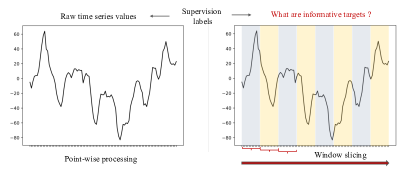
Figure 1: A toy example of time series processing comparison between previous point-wise processing (left) and our window slicing (right).

Masked autoencoders [23, 24], which can well overcome these aforementioned limitations, have been proposed before, whose main philosophy is to encode the masking-style corrupt input into latent space followed by a recovery of the raw inputs via the encoder and decoder. One successful instantiation is BERT [16], which is built based on a transformer network and has achieved a great milestone in representing language. Inspired by that, we notice that a pioneering work [25] has been presented based on transformer networks, which directly treats the raw time series as inputs, followed by recovering these full inputs with point-wise regression optimization. However, this methods often require very expensive computation cost due to ignoring the quadratic computation complexity incurred by self-attention mechanism [26, 27]. As reported by recently proposed methods [28, 29, 21], it seems that this method only produces limited representation results due to its weak generalization performance. In our view, such inferior generalizable performance is mainly caused by ignorance of the distinct properties of time series. First, unlike language data, time series are natural sequence signals with temporal redundancy, i.e., each time step can be easily inferred from its neighboring points. As a result, the pre-training representation encoder model cannot be well-trained due to the naive property of the recovering task. Second, since discriminative patterns in time series often exhibit in the form of sub-series (shapelet [5, 30]), each single point value can only carry very sparse semantic information as illustrated in left part of Figure 1. Lastly, it would also incur discrepancies between self-supervised pre-training and target task optimization due to the adoption of masking strategies. That is, a certain proportion of positions are replaced with masked embeddings while these artificial symbols are typically absent at the fine-tuning stage.

To address these aforementioned issues, in this work, we propose a novel masked autoencoder architecture, referred to as TimeMAE, for learning transferrable time series representations based on transformer networks. Specifically, instead of modeling each time step individually, we propose to split each time series into a sequence of non-overlapping sub-series with a window-slicing operation. Such a strategy not only increases the information density of the masked semantic units but also considerably saves the computation cost and memory consumption because of the shorter sequence length. The right part of Figure 1 shows a toy example of the window slicing partition. After window slicing, we perform masking operations over these redefined semantic units with the goal of bidirectional encoding of time series representations. Particularly, we find that the simple random masking strategy equipped with a very high proportion of $60\%$ matches well with the optimal representations of time series. Nevertheless, such a window slicing operation and masking strategies also easily incur some challenges. Accordingly, to solve the discrepancy incurred by masked positions, we design a decoupled autoencoder architecture, in which contextual representations of visible (unmasked) and masked regions are respectively extracted by two different encoder modules. To fulfill the recovery task, we formalize two pretext tasks to guide the pre-training process. One is the masked codeword classification (MCC) task of assigning each masked region its own discrete codeword, which is produced by an additionally designed tokenizer module. The other one is the masked representations regression (MRR) task, aiming at aligning the predicted representations of masked positions with the extracted target representations. Here, we employ a siamese network architecture to implement the generation of target representations for each masked position. Extensive experiments are performed on five public datasets. The experimental results clearly show that the pre-trained TimeMAE outperforms both from-scratch encoder and previous competitive baselines.

To sum up, we describe the contributions of the proposed TimeMAE as follows:

• We present a conceptually simple yet very effective self-supervised paradigm on time series representations, which prompts basic semantic elements from point granularity to localized sub-series granularity and facilitates contextual information extraction from unidirectional to bidirectional, simultaneously.

• We propose an end-to-end decoupled autoencoder architecture for time series representations, in which (1) we decouple the learning of masked and visible input so as to eliminate the discrepancy issues incurred by masked strategies; (2) we formalize two pretext tasks of recovering missing parts based on visible inputs, including the MCC and MRR tasks.

• We conduct extensive experiments on five publicly available datasets to verify the effectiveness of the TimeMAE. The experimental results clearly demonstrate the effectiveness of the newly formulated self-supervised paradigm and the proposed decoupled autoencoder architecture.

2 Related Work

In this section, we briefly introduce previous works closely related to our work from two branches: time series classification and self-supervision for time series.

2.1 Time Series Classification.

Numerous efforts have been devoted to the classification of time series over the past few years. In general, previous works can be roughly classified into two categories: pattern-based and feature-based. The former type typically extracts bag-of-patterns and then feeds them into a classifier [5, 31]. The effectiveness of these types of methods has been proved in many related advancements [32]. However, the greatest limitation of these works is that their computation cost is strictly coupled with the number of time series examples and sequence length, being the main bottleneck in real applications [33]. In contrast to the pattern-based methods, feature-based approaches are usually more efficient but their performance greatly depends on the quality of feature representations [34, 35]. Recently, the superiorities of deep learning-based methods have been proved in feature representation learning, in which less prior knowledge is used. Many complicated neural networks, such as recurrent neural networks, convolutional neural networks [6, 4, 36], and self-attentive-based models, have been applied for time series classification tasks. Besides, mining graph structure among time series with graph convolutional networks for comprehensive analysis have also attracted some researchers [37]. However, these deep learning-based methods typically require massive amounts of training data to achieve their optimal expressive capacity. Since it is hard to obtain numerous labeled data, directly using deep neural architecture might not bring satisfactory results.

2.2 Self-supervision for Time Series

Currently, self-supervised pre-training paradigms have nearly become the default configuration in the domains of natural language (NLP) [15, 16, 23] and computer vision (CV) [18, 17, 24]. Due to the unique property of time series, self-supervised learning for the time series pose particular challenges from those in CV and NLP. Hence, numerous efforts have been devoted to developing self-supervision methods for time series, in which the current works mainly obey two paradigms: reconstructive [38, 16, 39] and discriminative [40, 41, 42]. The idea of reconstructive methods try to recover the full input by the relies on autoencoders. E.g., TimeNet [43] first leverages an encoder to convert time series into low-dimensional vectors, followed by a decoder to reconstruct the original time series based on recurrent neural networks. Another representative reconstructive method is TST [25], whose main idea is to recover these masked time series points by the denoising autoencoder based on the transformer architecture. Whereas, the reconstructive optimization is modeled at a point-wise level, leading to very expensive computation consumption and limited generalizability [28]. In contrast, less computation consumption is required in discriminative methods [28], whose main solution is pulling positive examples together while pushing negative examples away [44]. A common underlying theme among these methods is that they all learn representations with data augmentation strategies [45], followed by maximizing the similarity of positive examples using a siamese network architecture. The key efforts are devoted to solving the trivial constant solutions [17] via various negative sampling strategies. For instance in T-Loss [46], time-based negative sampling with triple loss is utilized, simultaneously. TNC [8] leverages local smoothness of time series signal to treat sub-series neighborhoods as positive examples while regarding non-neighbor regions as negative instances. TS-TCC [28] uses both point-level and instance-level contrasting optimization objectives to align the corresponding representations. The distinct characteristic of TS2Vec [29] is hierarchically performing contrasting optimization across multiple scales. Moreover, the assumption of consistency between time and frequency domain is used in [21]. To sum up, the objective of these contrastive learning methods is trying to learn features that are invariant to distortions of various augmented inputs  [20, 13]. However, not only the data augmentation strategy requires many inductive biases but also the invariance assumption is not always existed.

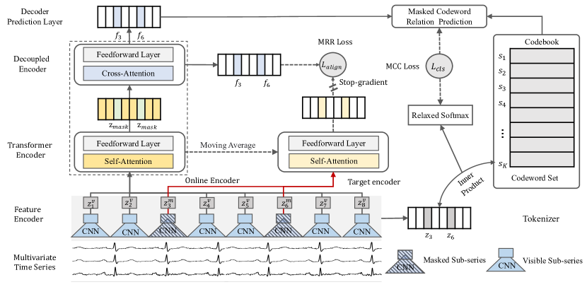
Figure 2: Overall architecture of the proposed TimeMAE—a decoupled masked autoencoder architecture, jointly optimized with two pretext task including the masked codeword classification and masked representation regression tasks.

3 The Proposed TimeMAE Model

In this section, we first formally describe the used notations and the studied problems. After that, we briefly introduce the overall pre-training architecture of the TimeMAE. Then, we introduce the pre-training architecture beginning from feature encoder layer, representation layer, to pretext optimization task, in detail.

3.1 Problem Definitions

We introduce these used notations and the problem definition. $\mathbb{D}={(X^{1},y^{1}),(X^{2},y^{2}),...,(X^{n},y^{n})}$ is a dataset containing a collection of pairs $(X^{i},y^{i})$, in which $n$ denotes the number of examples and $X^{i}$ denotes the univariate or multivariate time series with its corresponding label denoted by $y^{i}$. We represent each time series signals as $X=[x_{1},x_{2},...,x_{T}]\in\mathbb{R}^{m\times T}$ where $m$ is the number of channels and $T$ is the number of measurements over time. Given a set of unlabeled time series data, self-supervised learning for time series aims to obtain transferrable time series representations, which can facilitate the capacity of time series classification tasks.

3.2 Overview of the Pre-training Architecture

As depicted in Figure 2, we demonstrate the overall architecture of the pre-training process in the TimeMAE model. First, we project the input series into latent representations, followed by masking strategies to divide the whole input into visible (unmasked) inputs and masked sub-series. Then, we adopt a decoupled autoencoder architecture to learn the representations of visible and masked positions with two corresponding encoders. At the encoder level, we employ a set of vanilla transformer encoder blocks to extract contextual representations of visible inputs, while leveraging several layers of the cross-attention-based transformer encoder network to learn the representations at masked positions. At the decoder level, we perform the reconstructing task by predicting all missing parts based on visible inputs with the help of two types of newly constructed target signals. For one thing, we add a tokenizer module to assign each masked region its own codeword, allowing the codeword classification task to be trained. For another, we employ a siamese network architecture to generate continuous target representation signals, aiming at performing the target representation regression task. In the next, we elaborate on the design of the TimeMAE model.

3.3 Feature Encoding Layer

In this subsection, we mainly answer two vital questions during masking operation: how to choose well-informative basic semantic units for pre-training and how to achieve the goal of the bidirectional encoder of time series?

3.3.1 Window Slicing Strategies

For most of the existing works [47, 28], processing time series in a point-wise manner has nearly become the default paradigm for encoding time series into representation space, in which each time series point is individually modeled in capturing sequence dependence. In our view, we argue such point-wise style modeling largely restricts the capacity of self-supervised learning in time series. To be more specific, such a setting roughly ignores the difference between the information density of masked words and masked time series points. In contrast, the former type is generated by human and typically preserve very enriched semantic information while the latter type only involves sparse semantic features. Meanwhile, there exists great temporal redundancy among neighboring points of time series data, which means that each masked point can be easily inferred from its neighboring points without too much challenge. Consequently, the pre-trained encoder can only carry limited information during such a trivial reconstruction process. These analyses naturally motivate us to tap the potential of masking input modeling by increasing the information density of basic semantic units. Hence, we propose to leverage the local pattern property of time series, allowing sub-series as basic modeling elements rather than point-wise inputs. Accordingly, each time series can be processed into a sequence of sub-series units, in which each localized sub-series region preserves more enriched semantic information and can ensure the challenge of the reconstruction task. Note that such an argument can be also supported by the shapelet-based models [48], in which many discriminative sub-series related to the class labels are extracted as useful pattern features for the classification of time series. For example, we need to identify the anomaly ECG signals [49] via many local regions of waveform rather than the single point.

To be precise, we can use a slicing window operation to segment the raw time series into continuous non-overlapping sub-series. Formally, for a given time series $X=\{x_{1},x_{2},...,x_{T}\}\in\mathbb{R}^{T\times m}$, a slice is a snippet of the raw time series, defined as $s_{i:j}=\{x_{i},x_{i+1},...,x_{i+\sigma}\}$. Here, $\sigma$ denotes the size of the slicing window. Suppose the length of the given time series $X$ is $T$, our slicing operation will reduce it to a new length of $\lceil\frac{T}{\sigma}\rceil$. Padding with zero operation will be performed to ensure the fixed sequence length. In our implementation, we process the whole time series into a sequence of regular non-overlapping sub-series patches. The main reason behind this is such a setting can ensure the visible regions do not contain information about the reconstructed ones. Before modeling the sequence dependence of these sub-series units, we need to encode each element into latent representations by feature encoder. Here, we employ a $1$-D convolution layer to extract local pattern features across channels. It should be noted that different sub-series share the same project parameters during feature encoder layer. Projected hidden representations of the input $X$ are denoted by $Z=[z_{1},z_{2},...,z_{\lceil\frac{T}{\sigma}\rceil}]\in\mathbb{R}^{\lceil\frac{T}{\sigma}\rceil\times d}$, where $d$ is the dimension of the hidden representation. We use $S$ to indicate the new sequence length $\lceil\frac{T}{\sigma}\rceil$ while using $S_{v}/S_{m}$ to denote the number of visible /masked positions.

3.3.2 Masking Strategies

To achieve the goal of learning contextual representations of time series with a bidirectional encoding scheme, we decide to construct the corrupt input with masking strategies by following [16]. Suppose that $S_{v}/S_{m}$ is the number of masked/visible positions. In this way, more comprehensive contextual representations of each position, including previous and future contexts, can be encoded, simultaneously. For clarity, we use $Z_{v}$ to denote the embeddings of visible (unmasked) positions while letting $Z_{m}$ be the embeddings of masked ones. Although some heuristic masking strategies, e.g., block masking [23], have been developed before, we adopt random masking strategies to form the corrupted inputs. It means that each sub-series unit has the same probability of being masked in constructing self-supervised signals. The main reason that is such a strategy is beneficial to ensure that the representation quality of each input position is fully improved during reconstruction optimization. Note that we dynamically mask the time series at random for each pre-training epoch to further increase the diversity of the training signals. In addition to random masking operation, preserving a higher masking portion is also encouraged in the TimeMAE. This is because the masking ratio plays a vital role in deciding whether the recovering task is challenging enough to help the encoder carry more information. Generally, a higher masking ratio means that the recovering task is harder to be solved by the relies on these visible neighboring regions. Accordingly, more expressive network capacity can be encoded in the pre-trained encoder network. In our work, we find that a masking ratio of about $60\%$ can help us achieve optimal performance, greatly different from the masking ratio of $15\%$ in previous works [16, 25]. Note that both the window slicing and masking strategy are agnostic to the time series input, which does not bring too much inductive bias like data augmentation in contrastive learning [28].

3.4 Representations Learning for Time Series

In this section, we introduce the representation learning layer for complicated sequence dependence modeling. Particularly, the key design our TimeMAE is to employ two different encoder modules to learn the representation of visible positions and masked ones, respectively. Such a decoupling setting is beneficial to mitigate the discrepancy issue caused by additionally masked embeddings between pre-training optimization and fine-tuning training. Next, we introduce them in detail.

3.4.1 Representing Visible Positions

In the TimeMAE, we adopt the vanilla transformer encoder architecture denoted by $\mathcal{H}_{\theta}$, consisting of multi-head attention layers and feed-forward network layers, to learn contextual representations of input at visible regions. With such an architecture, the representation of each input unit can obtain the semantic relation of all other positions through the self-attention computation mechanism. It should be noted that the bottleneck of leveraging self-attentive architecture for long sequence input has been largely mitigated by our window slicing operation. Due to the permutation-equivalent self-attention computation, we thus add relative positional embeddings $P\in\mathbb{R}^{S\times d}$ to each position of sub-series embedding so as to preserve the order of sequence properties. Accordingly, the input embeddings can be reorganized by combining the positional encodings $P$ and the projected representations $Z$, i.e., $Z=Z+P$. Then, we send the input embeddings at visible positions $Z_{v}$ into the encoder $\mathcal{H}_{\theta}$. There are $L_{v}$ layers of transformer block in our model, and the output of the last layer $\mathcal{H}_{\theta}^{L_{v}}=\{h_{1}^{L_{v}},h_{2}^{L_{v}},...,h_{S_{v}}^{L_{v}}\}$ represents the global contextual representation of $S_{v}$ visible positions. Unlike previous works, we only feed the representation of visible regions into the encoder network while removing those of masked positions. In this way, no masked embeddings are used to train the encoder network, so that the discrepancy between pre-training and fine-tuning tasks incurred by masked token inputs can be largely alleviated. That is, such strategies eliminate the dilemma of feeding masked tokens into the encoder module in the forward pass.

3.4.2 Representing Masked Positions

To obtain the representations of masked input units, we further replace the self-attention in the vanilla transformer encoder with cross-attention to form the decoupled encoder module, denoted by $\mathcal{F}_{\phi}$, which indicates the decoupling of representation learning between visible and masked inputs. Specifically, we send these representations at visible and masked positions into the decoupled encoder so as to represent the input units at masked positions. Note that the embedding at masked positions is replaced with a newly initialized vector $z_{mask}\in\mathbb{R}^{d}$ while keeping the corresponding positional embedding unchanged. For clarity, embeddings of the reinitialized masked regions are indicated by $\tilde{Z}$. During representation learning in the decoupled encoder, we treat the representations of masked positions as query embeddings, i.e., $\tilde{Z}$, while regarding the transformed embeddings of visible positions $\mathcal{H}_{\theta}^{L_{v}}$ as input to help form keys and values. Formally, the model parameters of masked queries $W^{Q_{m}}\in\mathbb{R}^{d\times d}$ are the same for all masked queries. The projection parameters of visible keys and values, i.e., $W^{K_{v}},W^{V_{v}}\in\mathbb{R}^{d\times d}$ are also shared with visible inputs. The $L_{m}$-th layer output of the decoupled encoder $\mathcal{F}_{\phi}^{L_{m}}=\{f_{1}^{L_{m}},f_{2}^{L_{m}},...,f_{S_{m}}^{L_{m}}\}$ represents the transformed contextual representations of $S_{m}$ masked positions. Note that the decoupled module solely makes predictions of embeddings of masked positions while maintaining the embeddings of visible ones not updated. The main reason is that we hope such an operation can help alleviate the discrepancy issue in the backward pass. By this segmentation operation, the representation role of visible input is only taken responsibly by the previous encoder $\mathcal{H}_{\theta}$. Meanwhile, the decouple encoder mainly focuses on the representation of masked positions. Furthermore, another advantage of the decoupled module $\mathcal{F}_{\phi}$ is to prevent the decoder prediction layer from making the representation learning of visible positions, so that the encoder module $\mathcal{H}_{\theta}$ can carry more meaningful information.

3.5 Self-supervised Optimization

As stated in  [50], directly formulating self-supervised signals would largely restrict the capacity of the representation model due to the noisy and unbound properties of raw space [50]. Next, we mainly aim to answer the question of representing informative targets for masked semantic units, so that the corresponding pretext tasks can be accomplished.

3.5.1 Masked Codeword Classification

With the window slicing operation, each time series are reformulated into a sequence of sub-series, which could exhibit more enriched semantics. Taking inspirations from product quantization [51], a natural idea is whether we can represent such reformulated series in a novel discrete view, i.e., assign each local sub-series with its own “codeword”. Then, these assigned codewords serve as surrogate supervision signals for missing parts. For most of the current product quantization methods, the main idea is to encode each dense vector with a short code composed of cluster index based on cluster operation, in which all indices form the codebook vocabulary. Though its approximation error is low, it is actually a two-stage method, i.e., independently assigning the clustered index the extraction of learned features. In this way, the representation capacity of the codebook might be incompatible with the extracted features from the transformer encoder and the decoupled networks. Because of such an incompatibility, the performance of self-supervised training will be directly get impaired if naively employing such techniques to assign discrete supervision signals. Hence, we decide to develop a tokenizer module, which can convert the continuous embeddings of masked positions into discrete codewords in an end-to-end manner. We name such type of reconstruction task masked codeword classification (MRR).

To be precise, we assume that the tokenizer is composed of a codebook matrix $C=\{c_{1},c_{2},...,c_{K}\}\in\mathbb{R}^{K\times d}$, consisting of $K$ latent vectors. Here, $c_{k}\in\mathbb{R}^{d}$ denotes the $k$-th codeword in the codebook. In addition, the indices of the codebook naturally form the supervision vocabulary $V=\{v_{1},v_{2},...,v_{K}\}$. The key idea is to assign the nearest codeword to each sub-series through similarity computation. Concretely, the codeword of each masked sub-series representation $z_{i}\in\mathbb{R}^{d}$ is approximately encoded as follows,

$$z^{m}_{i}\approx v_{k_{i}},s.t.k_{i}=\arg\max_{j}sim(z_{i},c_{j}),j\in[K],$$ (1)

where $sim(z_{i},c_{j})$ is a measurement function to evaluate the similarity between sub-series representation and candidate codeword vectors. Instead of using cosine similarity, we use inner product to estimate the relevance score in the tokenizer, since gradient explosion incurred the reciprocal of the norm can be easily prevented. In this way, each local sub-series can be assigned its own discrete codeword, representing the inherent temporal patterns. After assigning the codeword to each input unit, we pass the embedding matrix to the decoder layer to obtain the codeword prediction distribution $p(s_{k_{i}}|f_{i}^{L_{m}})$ so as to perform the MCC optimization. Although heavy decoders might result in greater generation capability, their great capability can only serve for prediction in pretext tasks and cannot benefit the target tasks during the fine-tuning process. Hence, we abandon the heavy decoder head design and only use the extremely lightweight prediction head — inner product as a measurement tool to obtain the similarity distribution between contextual representation and candidate codeword vectors.

Without loss of generality, we adopt cross-entropy loss [52] to form the class token recovering optimization $\mathcal{L}_{cls}$, which is written as,

$$\mathcal{L}_{cls}(q,p)=-q(s_{k_{i}}|z_{i})\log p(s_{k_{i}}|f_{i}^{L_{m}})$$ (2)

where $q(s_{k_{i}}|z_{i})\in[0,1]^{K}$ denotes one-hot encoding obtained by the maximum selection of in codeword assignment. The optimization goal in Equation 2 is equal to maximizing the log-likelihood of the correct codewords given the masked input embeddings. However, it is reported that this codeword maximum selection operator easily leads to two aspects of issues: (1) it is easy to lead to the collapse results [53], i.e., only very few ratios of codewords are selected; (2) it makes it non-differentiable for the optimization loss in the above equation so that the back-propagation algorithm cannot be applied to computing gradients.

To solve these issues, we hence relax the maximum by tempered softmax combined with a prior distribution. Formally, the probabilities of selecting $k$-th codeword can be described as follows

$$q(v_{k}|z_{i})\approx\tilde{q}(v_{k}|z_{i})=\dfrac{\exp((sim(z_{i},c_{k})+n_{k})/\tau)}{\sum_{k^{\prime}\in K}\exp((sim(z_{i},c_{k^{\prime}})+n_{k^{\prime}})/\tau)},$$ (3)

in which $\tau$ is a temperature factor, controlling the degree of approximation. For example, the approximation becomes exact if $\tau\rightarrow 0$, whereas $\tilde{q}$ is close to the uniform distribution when $\tau$ is too large. In addition, $n=-\log(-\log(a))$ and $a$ is uniform samples from $\mathcal{U}(0,1)$. In our implementation, we adopt Gumbel prior distribution to implement $\mathcal{U}$ by following [54, 55]. With such a designed relaxed softmax, the maximum selection is replaced by approximately sampling from the probability distribution so that the collapse issue can be largely alleviated.

To solve the non-differentiable issue, by following the trick of Straight-Through Estimator (STE) in [56], we mimic the gradient updating by rewriting $b_{j}$ as follows,

$$\hat{q}(v_{k}|z_{i})=\tilde{q}(v_{k}|z_{i})+sg(q(s_{k}|z_{i})-\tilde{q}(s_{k}|z_{i})),$$ (4)

where $sg$ denotes the stop gradient operator, i.e., zero partial derivatives, which can effectively constrain its operation to be a non-updated constant. In the forward pass, the stop gradient does not work, i.e., $\hat{q}(v_{k}|z_{i})=q(v_{k}|z_{i})=$$\rm one\_hot$$(\arg\max_{j}sim(z_{i},c_{j}))$. During the forward pass, the index of the nearest embedding is assigned as the current embedding vector’s discrete codeword. During the backward pass, the stop-gradient operation takes effects, i.e., $\nabla_{\hat{q}(v_{k}|z_{i})}=\nabla_{\tilde{q}(v_{k}|z_{i})}$. Accordingly, the gradient $\nabla\mathcal{L}_{cls}$ is passed unaltered to the embedding space of the codebook matrix, which means that the non-differentiable issue is solved. Note that the gradients contain useful information about how the encoder should change its output to lower the reconstruction loss, which ensures the enriched semantics of each codeword. During each epoch, the gradient can push the embeddings of masked regions to be tokenized differently in the next forward pass, because the assignment in Equation 1 will be different.

3.5.2 Masked Representations Regression

In addition to making predictions of the discrete codeword, we are interested in directly performing regression optimization in the latent representation space. We refer to such a pretext task as the masked representation regression (MRR) optimization. Such an idea is mainly motivated by the fundamental principles of representation learning — the space of hidden factors that characterize the underlying distribution of the data is of a much lower dimension than the original space as stated in [57]. Meanwhile, latent representation space allows focusing on important features of the raw time series while being less sensitive to noise [58]. To fulfill this objective, we choose to use the well-known siamese network architecture, which is widely used for self-supervised contrastive learning optimization. The main idea of contrastive optimization is to try to pull the representations of positively-related instances close while pushing those of negative-related ones far away from each other. Different from this typical contrastive optimization [18, 29], the MRR task can be viewed as a special case without leveraging negative instances during training.

To generate the target representations, a novel target encoder module is further adopted. Let $\mathcal{H}_{\xi}$ denote the target encoder, which preserves the same hyper-parameter setting as the encoder of $\mathcal{H}_{\theta}$ but parameterized with $\xi$. To facilitate the understanding, we name the combination of the vanilla transformer encoder and the decoupled encoder modules as online encoder, in which aligned representations are generated. Relying on such a siamese network architecture, different views of the masked sub-series representations can be produced by the target encoder and online encoder, respectively. Accordingly, aligning the corresponding representation of two different views, i.e., target representations $\mathcal{H}_{\xi}^{L_{v}}(Z_{m})$ and predicted representations $\mathcal{F}_{\phi}^{L_{m}}(\tilde{Z})$, naturally form the goal of MRR task. Given continuous representation as regression signals, we adopt the mean squared error (MSE) loss to form the specific optimization objectives. Subsequently, we define the exact regression optimization loss as follows,

$$\mathcal{L}_{align}=\parallel\mathcal{H}_{\xi}^{L_{v}}(Z_{m})-\mathcal{F}_{\phi}^{L_{m}}(\tilde{Z})\parallel_{2}^{2}.$$ (5)

Theoretically, the gradient of loss in Equation 5 can be employed to optimize both the online encoder and target encoder. Since the negative example is omitted in the siamese network architecture, however, it is easy to incur collapse solution [53]. To prevent the model collapse results, we can obey the rule of updating two networks differently, whose effectiveness has been proved to be effective in previous works [18]. Following this idea, we perform a stochastic optimization step to only minimize the parameters of the online encoder while updating the target encoder in a momentum moving-average manner. Particularly, we describe the exact updating manner of the target encoder as follows,

$$\begin{split}\xi&\leftarrow\eta\cdot\xi+(1-\eta)\cdot\theta,\\ \theta&\leftarrow\theta-\gamma\cdot\nabla_{\theta}\mathcal{L}_{align},\\ \phi&\leftarrow\phi-\gamma\cdot\nabla_{\phi}\mathcal{L}_{align},\\ \end{split}$$ (6)

in which $\eta\in[0,1]$ is a momentum coefficient for the momentum-based moving average. With a large value of $\eta$, the target encoder slowly approximates the encoder $\mathcal{H}_{\theta}$. In the TimeMAE, we find $\eta=0.99$ performs effectively. Further, $\nabla_{\cdot}$ is the gradient and $\gamma$ denotes the learning rate for stochastic optimization. As shown in Equation 6, the direction of updating target encoder $\mathcal{H}_{\xi}$ completely differs from that of updating the $\mathcal{H}_{\theta}$ and $\mathcal{F}_{\phi}$. Finally, $\mathcal{H}_{\xi}$ converges to equilibrium by the slow-moving average. To be more specific, at each training step, the optimization direction of the online encoder and target encoder are decided by gradient produced by $\mathcal{L}_{align}$ and $\xi-\theta$. By doing so, the problem of model collapse can be effectively solved with such different updating manners.

3.5.3 Multi-task Optimization

In the pre-training stage, our TimeMAE is trained in a multi-task manner by combing the MCC and MRR tasks together. Precisely, the overall self-supervised optimization objectives of the pre-training model can be written as,

$$\mathcal{L}=\alpha\mathcal{L}_{cls}+\beta\mathcal{L}_{align},$$ (7)

where $\alpha,\beta$ are the tuned hyper-parameters, controlling the weight of two losses. Stochastic gradient optimization combined with a mini-batch training algorithm can be employed to optimize the above joint loss. Coupling both masked token modeling and target representation alignment tasks enables the pre-trained model to get better generalization performance for target downstream tasks. Through joint self-supervised optimization, transferrable pre-trained models can be effectively learned so as to benefit the target task.

4 Experiments

In this section, we first introduce the setups of our TimeMAE, including the pre-training and fine-tuning stages. Then, we compare the experimental results of all compared methods over the classification of time series. Also, we report some insightful findings to deeply understand the proposed TimeMAE.

4.1 Experimental Setup

4.1.1 Datasets

We conduct experiments on five publicly available datasets, including human activity recognition (HAR), PhonemeSpectra (PS), ArabicDigits (AD), Uwave, and Epilepsy, which are provided by [59, 60, 28, 61]. These five datasets cover a wide range of variations: different numbers of channels, varying time series lengths, different sampling rates, different scenarios, and diverse types of time series signals. It should be noted that we do not make any processing on these datasets because the original training and testing set have been well processed. In addition, Table I summarizes the statistics of each dataset, e.g., the number of instances (# Instance), the sequence length (# Length), the number of channels (# Channel), and the number of classes (# Class).

4.1.2 Compared Methods

To demonstrate the effectiveness of our TimeMAE, we compare it to some popular self-supervised time series representation methods. We compare our methods to the following baselines in the experiments:

• FineZero means that we train the vanilla transformer encoder networks from scratch without the help of a self-supervised pre-training process.

• TST [25] processes the time series in a point-wise style and formulates the regression of raw time series as self-supervised optimization.

• TNC [8] employs a debiased contrastive objective, in which the distribution of signals from within a neighborhood is distinguishable from the distribution of non-neighboring ones.

• TS-TCC [28] learns unsupervised time series representations from unlabeled data via leveraging both point-level and instance-level contrasting optimization objectives in a unified framework.

• TS2Vec [29] mainly performs contrastive optimization in a hierarchical manner over augmented views with various scales.

TABLE I: Statistics of five used datasets in experiments.

Dataset	# Example	Length	# Channel	# Class
HAR	11,770	128	9	6
PS	6,668	217	11	39
AD	8,800	93	13	10
Uwave	4,478	315	3	8
Epilepsy	11,500	178	1	2

In addition to the comparison baselines listed above, for a fair comparison, we replace the point-wise input processing in the training encoder with newly designed window slicing strategies, denoted by FineZero+. Because our goal is to compare the performance of self-supervised learning models that are independent of the encoder network settings. To eliminate the influence of encoder architecture, we follow the setting in [8] and maintain the same transformer encoder architecture in [16] for all compared methods.

4.1.3 Pre-training and Fine-tuning Setup

In our experiments, we demonstrate the effectiveness of pre-trained model parameters with two mainstream evaluation manners: linear evaluation and fine-tuning evaluation. The former manner means the parameters of the pre-trained encoder are frozen, whereas only the newly initialized classifier layer is tuned according to the labels of target tasks. The latter manner denotes that the parameters of pre-trained encoders and the newly initialized classifier layer are tuned without any frozen operation. These two evaluation manners are denoted by FineLast and FineAll, respectively. Relatively speaking, the measurement of FineLast manner could further reflect the quality of pre-trained models. For the time series classification task, we require the entire instance-level representation. As such, we use mean pooling over all temporal points to denote the whole time series, followed by a cross-entropy loss to guide the optimization of models in the training stage of downstream tasks. To better evaluate the imbalanced datasets, the metrics of accuracy and macro-averaged F1 Score are employed as the evaluation metrics of time series classification tasks. The best results are highlighted in boldface. In default settings, all results of Accuracy and F1 Score in this table are denoted in the percentage (%). Reported experimental results are mean and standard deviation values across three independent runs on the same data split.

TABLE II: Comparison of the TimeMAE model against competitive baselines in terms of both metrics of FineLast and FineAll over five datasets.

Metrics	FineLast & Accuracy					FineAll &Accuracy
Datasets	HAR	PS	AD	Uwave	Epilepsy	HAR	PS	AD	Uwave	Epilepsy
FineZero	68.02±0.84	6.92±0.34	80.27±3.18	88.35±0.27	92.26±0.13	89.73±0.42	8.98±0.54	98.68±0.09	97.38±0.25	97.14±0.13
FineZero+	66.53±0.70	7.98±0.27	69.45±3.95	87.56±0.28	95.05±0.31	92.26±0.47	17.03±0.52	98.53±0.18	97.35±0.23	98.92±0.07
TST	87.39±0.27	8.93±0.58	96.03±0.44	95.17±0.51	96.19±0.09	94.35±0.11	8.82±0.30	99.06±0.39	97.98±0.12	96.91±0.11
TNC	87.82±0.18	10.05±0.52	92.38±1.27	91.36±0.60	97.17±0.09	92.02±0.75	10.58±0.25	98.24±0.47	97.06±0.20	97.43±0.05
TS-TCC	77.63±0.20	8.88±0.39	88.42±1.52	91.76±0.43	95.21±0.15	89.22±0.19	8.47±0.68	98.71±0.09	97.32±0.28	96.83±0.05
TS2Vec	78.16±0.80	10.82±0.38	94.65±0.30	92.76±0.34	97.13±0.15	86.98±2.17	10.07±0.66	99.11±0.23	96.69±0.21	96.99±0.11
TimeMAE	91.31±0.10	19.25±0.22	95.76±0.51	95.88±0.28	97.88±0.20	95.11±0.18	20.30±0.27	99.20±0.03	98.37±0.12	99.35±0.19
	FineLast & F1 Score					FineAll & F1 Score
FineZero	66.39±1.04	6.18±0.31	80.10±3.13	88.27±0.28	87.99±0.20	89.72±0.39	8.47±0.50	98.68±0.09	97.38±0.25	95.54±0.18
FineZero+	64.65±0.83	7.44±0.30	68.95±4.24	87.46±0.28	92.12±0.49	92.27±0.46	15.33±0.43	98.53±0.19	97.35±0.24	98.33±0.10
TST	87.18±0.29	7.71±0.78	96.02±0.44	95.16±0.51	93.96±0.20	94.33±0.07	7.79±0.91	99.06±0.39	97.98±0.13	95.18±0.16
TNC	87.63±0.19	8.72±0.22	92.35±1.29	91.34±0.60	95.64±0.15	91.89±0.79	9.26±0.52	98.24±0.47	97.05±0.20	96.04±0.07
TS-TCC	77.09±0.14	7.54±0.35	88.41±1.55	91.71±0.48	92.34±0.22	89.04±0.15	8.00±0.54	98.71±0.09	97.34±0.28	95.09±0.07
TS2Vec	77.43±0.91	10.09±0.26	94.64±0.31	92.71±0.33	95.58±0.25	86.69±2.38	8.63±1.06	99.10±0.23	96.70±0.21	95.26±0.22
TimeMAE	91.25±0.06	18.18±0.27	95.75±0.51	95.87±0.29	96.66±0.35	95.10±0.17	18.83±0.72	99.20±0.03	98.39±0.12	98.85±0.24

TABLE III: Transferring learning performance comparison between the TimeMAE and several other baselines, in which only experimental results of FineAll evaluation manner is reported due to the cross-domain setting. The best results are highlighted in boldface.

Models	Accuracy				F1 Score
	PhonemeSpectra	ArabicDigits	Uwave	Epilepsy	PhonemeSpectra	ArabicDigits	Uwave	Epilepsy
FineZero	8.98±0.54	98.68±0.09	97.38±0.25	97.14±0.13	8.47±0.5	98.68±0.09	97.38±0.25	95.54±0.18
FineZero+	7.98±0.27	69.45±3.95	87.56±0.28	95.05±0.31	17.03±0.52	98.53±0.18	97.35±0.23	98.92±0.07
TST	9.43±0.31	98.71±0.21	97.24±0.48	97.18±0.08	7.77±0.34	98.71±0.22	97.26±0.48	95.61±0.08
TNC	9.43±0.75	98.56±0.05	96.98±0.56	97.07±0.18	8.28±0.79	98.56±0.05	96.99±0.55	95.48±0.28
TS-TCC	9.46±0.28	98.50±0.08	97.48±0.08	97.11±0.13	8.20±0.37	98.50±0.08	97.48±0.07	95.54±0.16
TS2Vec	6.52±0.10	98.62±0.12	96.85±0.14	96.73±0.22	4.30±0.10	98.62±0.12	96.86±0.12	94.82±0.25
TimeMAE	18.53±0.69	98.76±0.07	97.72±0.08	99.08±0.12	17.21±0.43	98.76±0.07	97.73±0.08	98.76±0.16

4.1.4 Implement Details

In the pre-training stage, we consistently regard the embedding size as $64$ in all models. Adam optimizer is employed as the default optimizer for all compared methods. The learning rate is set to $0.001$ without any additional tricky settings. The batch size is set to $64$ for all models. By default, the layer depth of the utilized transformer encoder architecture is set to $8$, in which the number of attention heads is $4$, a two-layer feed-forward network is adopted, and the dropout rate is $0.2$. For several competitive baselines, we strictly follow the corresponding hyper-parameter settings and data augmentation strategies suggested by the original work [25, 8, 28, 29]. In addition to the used transformer encoder, we also use a six-layer decoupled encoder to extract contextual representations of masked positions. For each dataset, the used slicing window size $\delta$ is searched from $\{4,8,12,16\}$. In the default setting, we adopt the masking ratio of $60\%$ for our TimeMAE model. Within the MCC task, the vocabulary size of the codebook in our designed tokenizer is searched from $\{64,96,128,192,256,512\}$ for the specific dataset. As for the MRR task, the $\tau$ is set to $0.99$. To obtain the optimal trade-off between two pretext tasks, we fix the $\alpha$ as $1$ while searching the suitable values of $\beta$ ranging from $\{1,2,...,10\}$. Note that we preserve the same hyper-parameter settings as the pre-trained model while involving the overlapping hyper-parameters in the fine-tuning stage. The source codes of our TimeMAE are available at https://github.com/Mingyue-Cheng/TimeMAE.

4.2 Experiment Results

4.2.1 One-to One Pre-training Evaluation

In this section, we demonstrate the effectiveness of our approach against the competitive baselines in terms of one-to-one pre-training paradigm. Specifically, we first perform self-supervised pre-training without using annotated labels, followed by a retraining stage tuned with labeled datasets for classification tasks. Finally, the model’s performance is evaluated in the testing set.

Table II shows the classification results, we observe that the classification performance of compared methods evaluated by FineAll manner can be more promising than that evaluated by FineLast manner. This is reasonable because the FineAll evaluation fully force the whole model parameter to adapt to target tasks. In contrast, only the last classifier is tuned according to the target label in the evaluation manner of FineLast. In both metrics, our TimeMAE achieves substantial performance improvements compared to other baselines in most situations. In particular, the capacity of our TimeMAE in terms of linear evaluation could outperform supervised learning version baselines on the HAR and PS datasets, which fully demonstrates the powerful representation learning capacity of our TimeMAE model. We attribute such success to the simple philosophy of recovering missing sub-series patches based on the visible inputs without relying on too much inductive bias like the data augmentation strategies in contrastive-based baselines. Among these baselines, it seems that there exist no apparent winners for all datasets. It is worth noting that masking-based autoencoders like baseline—TST cannot achieve promising improvements in contrast to our TimeMAE model. We hypothesize the performance degradation is mainly led by the sparse basic semantic unit in processing the time series in a point-wise style. Such arguments can also be evidenced by the compared results between FineZero and FineZero+.

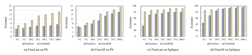
Figure 3: Comparison between FineZero+ v.s. our TimeMAE for different proportions of training set over two selected datasets, including PS and Epilepsy, in which both experimental results of FineLast and FineAll are reported.

TABLE IV: Performance analysis of the TimeMAE model with respect to varying sizes of encoder network, evaluated by FineLast and FineAll manners. Here, $l,d,n$ denote the layer depth of vanilla transformer encoder, the embedding size, and the number of pre-training epochs.

Evaluation	Datasets	Model Size	l = 8 d = 64 n = 100	l = 8 d = 64 n = 200	l = 8 d = 128 n = 200	l = 16 d = 64 n = 200	l = 16 d = 128 n = 100	l = 16 d = 128 n = 200
FineLast	HAR	Accuracy	91.31±0.10	91.99±0.12	92.63±0.64	91.97±1.81	91.40±0.44	92.82±0.31
		F1 Score	91.25±0.06	92.06±0.11	92.63±0.66	91.97±1.83	91.41±0.42	92.42±0.30
	PS	Accuracy	16.91±1.26	20.90±0.55	24.27±0.33	22.61±0.13	21.84±0.69	25.34±0.98
		F1 Score	15.72±1.19	19.81±0.54	23.88±0.36	22.00±0.17	21.39±0.62	25.02±0.84
	Epilepsy	Accuracy	97.88±0.20	98.56±0.16	99.04±0.14	98.91±0.18	98.88±0.08	99.33±0.06
		F1 Score	96.66±0.35	97.76±0.25	98.51±0.22	98.31±0.29	98.26±0.13	98.87±0.09
FineAll	HAR	Accuracy	95.11±0.18	94.98±0.75	95.19±0.16	95.43±0.52	95.08±0.08	95.51±0.65
		F1 Score	95.10±0.17	94.95±0.74	95.15±0.20	95.42±0.50	95.03±0.10	95.02±0.69
	PS	Accuracy	20.15±0.50	22.97±0.45	23.28±0.21	23.43±0.27	22.35±0.15	24.81±1.49
		F1 Score	18.86±0.52	21.97±0.48	22.15±0.95	22.37±0.78	20.76±0.40	23.97±1.52
	Epilepsy	Accuracy	99.35±0.19	99.46±0.11	99.41±0.19	99.57±0.01	99.41±0.08	99.52±0.03
		F1 Score	98.85±0.24	99.16±0.17	99.07±0.29	99.32±0.01	99.07±0.13	99.28±0.05

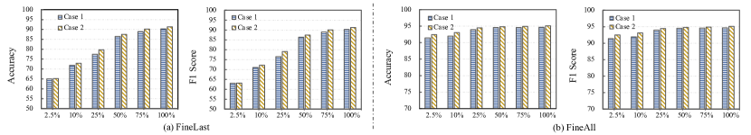
Figure 4: Performance analysis of the TimeMAE model with respect to different proportions of the pre-training set (i.e., x-axis) while preserving the same fine-tuning set within case 1 (70% of full training set) or case 2 (full training set).

4.2.2 Transferring Learning Evaluation

Recently advancements in self-supervised methods [39], have shown great potential for learning universal representations. Hence, to verify the generic capacity of the pre-trained model, we seek to investigate the transferability [62] of the pre-trained model by following one-to-many evaluation. To be more specific, self-supervised pre-training is done by using only one data followed by respectively fine-tuning multiple different target datasets. Out of five datasets, the HAR dataset has the largest number of examples. For that reason, we perform self-supervised pre-training on the HAR dataset and separately fine-tune the well-trained model on the remaining four datasets, including PS, AD, Uwave, and Epilepsy.

As shown in Table III, we report the classification performance in terms of metrics of FineLast and FineAll. We observe that the overall fine-tuning performance of our TimeMAE is slightly worse than the one-to-one evaluation setting. This is reasonable because there is less common properties between HAR and other several data signals, we expect the transferring learning will be less effective compared to fine-tuning within the same dataset. Among these compared methods, the TimeMAE could surpass all competitive baselines and achieve great performance by transferring learning. Meanwhile, some pre-trained representation models also can benefit the target task by transferring the learned model parameters. We hypothesize that the paradigm of masked sub-series modeling could learn the general-purpose representations. Such results indicate that our model has large potential to serve as a universal model for severing multiple different domains.

4.2.3 Fine-tuning with Varying Proportions of Training Set

One of the most valuable characteristics of pre-trained models is their stronger generalization in tackling the label sparse scenarios [39, 14]. We hence investigate the effectiveness of the TimeMAE model by simulating the data sparse scenarios with different proportions of training sets, i.e., $\{3\%,5\%,10\%,25\%,50\%,75\%,100\%\}$. It should be noted that all compared model variants preserve the same testing set to ensure a fair comparison. Accordingly, Figure 3 shows the evaluation results of FineZero+ and the TimeMAE on datasets of PS and Epilepsy. As we can see, the performance substantially drops when a lower proportion of training data is used. Notably, we find that our TimeMAE could achieve superior classification performance compared to randomly initialized models. Particularly in the dataset of Epilepsy, our TimeMAE could even achieve comparable classification performance tuned with very few labeled datasets as the capacity of randomly initialized version tuned with the full training set. This is meaningful in many scenarios of label sparse. Based on a very powerful pre-trained model foundation model, fewer training sets can help us achieve promising results.

TABLE V: Performance analysis of the TimeMAE model equipped with different sizes of slicing window.

Datasets	Evaluation	FineLast				FineAll
	Slicing Size	4	8	12	16	4	8	12	16
HAR	Accuracy	90.19±0.22	91.31±0.10	90.93±1.22	90.31±1.12	95.30±0.46	95.11±0.18	94.68±0.29	94.57±0.26
	F1 Score	90.14±0.21	91.25±0.06	90.87±1.31	90.27±1.14	95.28±0.48	95.10±0.17	94.66±0.33	94.55±0.31
PS	Accuracy	19.24±0.25	16.91±1.26	13.98±0.92	11.65±1.70	20.30±0.27	20.15±0.50	18.35±0.70	17.17±0.39
	F1 Score	18.17±0.27	15.72±1.19	12.85±0.84	10.64±1.61	18.83±0.72	18.86±0.51	17.73±0.42	15.98±0.23
Epilepsy	Accuracy	97.45±0.22	97.88±0.20	97.89±0.11	97.72±0.29	99.09±0.05	99.35±0.19	99.37±0.03	99.07±0.03
	F1 Score	95.99±0.35	96.66±0.35	96.68±0.18	96.42±0.46	98.58±0.09	98.85±0.24	99.03±0.04	98.55±0.05

TABLE VI: Performance analysis of the TimeMAE model equipped with different levels of masking ratio by gradually increasing from $20\%$ to $80\%$.

Evaluation	Datasets	Metrics	20.00%	30.00%	40.00%	50.00%	60.00%	70.00%	80.00%
FineLast	HAR	Accuracy	85.85±1.44	85.75±1.23	89.22±0.75	90.78±0.86	91.31±0.10	90.86±0.56	90.27±0.30
		F1 Score	85.63±1.50	85.53±1.37	89.09±0.72	90.75±0.84	91.25±0.06	90.79±0.50	90.21±0.34
	PS	Accuracy	13.21±0.56	14.24±0.37	14.33±0.65	14.29±0.42	14.36±0.20	15.80±1.06	16.91±1.26
		F1 Score	12.19±0.45	13.36±0.44	13.41±0.69	13.38±0.59	13.47±0.10	14.74±0.74	15.72±1.19
	Epilepsy	Accuracy	97.26±0.37	96.85±0.62	97.23±0.11	98.04±0.14	97.88±0.20	97.76±0.42	97.81±0.41
		F1 Score	95.67±0.62	95.02±0.96	95.61±0.17	96.93±0.22	96.66±0.35	96.49±0.69	96.56±0.70
FineAll	HAR	Accuracy	93.69±0.76	94.31±0.16	94.45±0.72	94.96±0.83	95.11±0.18	95.03±0.52	94.68±0.10
		F1 Score	93.70±0.72	94.28±0.20	94.43±0.69	94.94±0.85	95.10±0.17	94.98±0.56	94.66±0.11
	PS	Accuracy	17.93±0.41	18.86±0.84	18.95±0.70	19.17±0.53	19.60±0.21	19.33±0.64	20.15±0.50
		F1 Score	16.70±0.11	17.62±1.04	18.32±1.26	18.22±0.94	18.10±0.99	18.20±0.33	18.86±0.52
	Epilepsy	Accuracy	99.17±0.09	99.07±0.40	99.09±0.10	99.29±0.09	99.35±0.19	99.42±0.11	99.39±0.09
		F1 Score	98.72±0.16	98.55±0.64	98.56±0.14	98.90±0.13	98.85±0.24	99.10±0.17	99.05±0.15

4.2.4 Analysis of the Scalability about Model Size

In the area of self-supervised pre-training, a series of works [16] have revealed that stronger generalization models can be trained by scaling the scale of pre-trained encoder size or longer training. Inspired by that, we are interested in exploring whether similar performance can be found in representations of time series. Hence, we scale the model size of the encoder model by gradually varying the depth of encoder blocks ($8,16$), and the dimension of embedding size ($64,128$). Also, we control the number of epochs to verify whether longer pre-training can benefit the pre-training process. In our experiments, we totally set six different models, equipped with different hyper-parameter settings. We report the specific experimental results in Table IV. Overall, we observe that larger model sizes and longer pre-training epochs indeed can further generate more superior representation with slightly better generalization capacity on the HAR and Epilepsy datasets. In contrast, the bigger models obtain a significant performance gain on the PS datasets. This is probably because there are fewer pre-training sets on the PS dataset compared to the other two datasets. After all, a larger model should be matched well with more proportion of training set so as to fulfill the expressive capacity of networks. In the future, it is a promising direction to build a larger pre-training model as a foundation model to benefit time series classification tasks, e.g., by borrowing the idea of mixture of experts (MoE) [63].

4.2.5 Analysis of Varying Proportions of Pre-Training Set

Next, we wonder whether the proposed model would suffer from the saturation phenomenon [20] with increasing the pre-training set. That is, it cannot bring meaningful performance equipped with the increasing training sets for self-supervised learning if the pre-training approach encounters such saturation. Limited by the datasets, we investigate the effectiveness of the TimeMAE model by pre-training with varying proportions of the instance set while setting the same amounts of the tuned set. Specifically, we perform extensive experiments on the HAR dataset over two different version training sets ($100\%,70\%$) to fine-tune the pre-trained model, named Case $1$ and Case $2$, respectively. Figure 4 shows the results of our TimeMAE under the aforementioned experimental settings. We observe that the classification results of the target task could be further improved with the increase of the pre-training set, especially for metrics of linear evaluation manner. Such results are meaningful for real applications because the cost of collecting unsupervised time series data is much cheaper due to the omission of annotated efforts by domain experts. In this way, effective foundation models can be built via learning from a very large scale of unlabeled time series datasets to achieve more promising results for serving target tasks.

4.2.6 Study of Masking Strategies

One of the core ingredients of our TimeMAE is the combination of regarding the sub-series as a basic semantic unit and forming corrupted inputs by masking a certain proportion of positions. Hence, we study the effects of window slicing size and masking ratio for representation generalization. Note that all other hyper-parameter preserve the same setting due to the requirement of fair comparison. As shown in Table V and Table VI, we report the corresponding experimental results over three selected datasets. From these reported results, we have the following observations. First, one can see that both factors could significantly influence the generalization performance of pre-trained models. The former factor indicates how much semantics are involved in the basic semantic element. The latter factor means the challenging degree of recovering task. That is, these hyper-parameters factors could decide whether the recovering task over masked regions is challenging enough. Accordingly, the representation quality would be greatly affected equipped with different hyper-parameter settings. Second, the TimeMAE model is more sensitive to the masking ratio compared to the slicing window size on the HAR dataset, whereas such an influence trend is on the PS datasets. These findings largely reflect the great difference among datasets, which also bring great challenges in learning general-purpose time series representations.

4.2.7 Ablation Studies

In this part, we aim to perform an ablation analysis on the TimeMAE model. For one thing, we study the effects of the decoupled encoder by discarding the newly presented decoupled encoder, in which both visible and masked embeddings are passed into the same encoder. We name this type of model variant as w/o Decoupled. For another, we compare the experimental results of the TimeMAE model without optimization of the MCC/MRR task, denoted by w/o MCC and w/o MRR. In addition, we use Full Model to denote the TimeMAE model with default hyper-parameter settings. For saving space, we report the experimental results over the HAR and PS datasets as shown in Figure 5.

The Effects of Decoupled Setting. As we can see, the classification performance of the target task would degrade significantly while discarding the decoupled setting, which indicates the importance of decoupling the representations at the visible and masked sets. The main reason is easy to understand: the pre-training encoder with self-supervised optimization is involved with the masked embeddings while these embeddings are typically absent at the fine-tuning stage. As a result, it easily produces a great discrepancy between self-supervised pre-training and fine-tuning stages, so the representation capacity of the encoder is severely affected.

The Effects of Two Pretext Losses. From the results in shown figure, we observe that jointly leveraging two pretext tasks can force the encoder to achieve more optimal generalization performance on target tasks. It indicates that these two pretext tasks do not conflict one another and can work well together to increase the encoder module’s capacity for expressiveness. This is likely due to the fact that the MCC task predicts the discrete codeword, but the MRR task can be viewed as an optimization constraint for enhancing the encoder network’s capability. Additionally, we note that in these two selected datasets, the experimental outcomes optimized by the MRR task slightly outperform results of the MCC objective. We speculate that these outcomes may be a result of the codeword vector’s limited expressiveness. In the tokenizer, we only carry out retrieval operations from an initialized embedding matrix, i.e., codebook, which has a restricted capacity because there is no non-linear transformation. So strengthening the codebook’s representation quality is one way to potentially increase the TimeMAE.

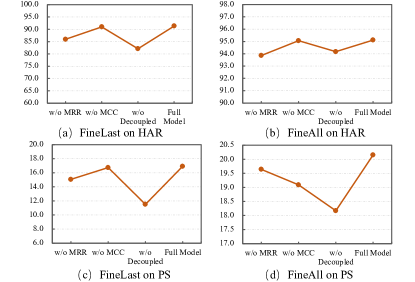
Figure 5: Performance analysis of the TimeMAE model equipped with jointly varying masking ratio and slicing window size, in which y-xis denotes the accuracy of compared methods.

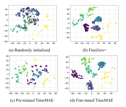
Figure 6: T-SNE visualizations of feature vectors on the HAR dataset, in which each color denotes a specific class category.

4.2.8 Visualization Analysis

Next, we aim to understand the proposed approach through visualization analysis. To conserve space, we use T-SNE [64] over the HAR dataset to display the learned features along with their labels. Figure 6(a) provides the visualization of features derived from randomly initialized encoders, while Figure 6(b) describes the visualization of features following supervision training without pre-training enhancement. Figures 6(c) and (d) show the visualization results of extracted features from a frozen pre-trained encoder and a fine-tuned one in TimeMAE. We draw the following observations from the visualization results: it is possible to separate well the extracted features from tuned TimeMAE and FineZero+. Among them, the Fine-tuned TimeMAE achieves better separation results. Such results demonstrate that our TimeMAE can help to guide the training of the encoder to represent each category in the latent representation space; (2) visualized features extracted from the pre-trained TimeMAE can also be well separated. Such results suggest that the pre-trained representations could largely reflect the underlying feature of raw time series data.

In Figure 7, we also visualize the learning curves of our TimeMAE and FineZero+ in terms of end-to-end fine-tuning evaluation, in which accuracy results are reported. On two selected datasets, as can be seen, pre-training with our TimeMAE greatly outperforms the random Initialization baseline in terms of accuracy and convergence speed. For instance, the FineZero+ requires at least $10$ epochs to converge to stable findings while the TimeMAE just needs three epochs to attain more superior classification performance.

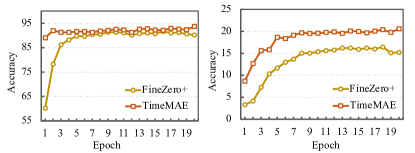
Figure 7: Visualization of learning curves in terms of FineZero+ and TimeMAE over HAR (left) and PS (right) datasets, in which we end-to-end fine-tune the whole model for both methods.

5 Conclusion and Future Work

In this work, we proposed a novel self-supervised model, named TimeMAE, for learning representations of time series based on transformer networks. The distinct characteristics of the TimeMAE are to adopt sub-series as basic semantic units with window slicing operation combined with masking strategies. Some novel challenges incurred by such a novel modeling paradigm are well solved. Specifically,to eliminate the discrepancy issue incurred by newly incorporated masking embeddings, we develop a decoupled autoencoder architecture. Furthermore, we construct two types of target signals to force the model to perform the reconstruction optimization objectives, including the masked codeword prediction (MRR) and the masked representation regression (MRR) tasks. With our TimeMAE, transferrable time series representations can be effectively learned by relying on the combination of more enriched basic semantic units and the bidirectional encoding strategy. We performed extensive experiments on five public datasets. The experiment results illustrate the effectiveness of the proposed TimeMAE by reporting some insightful findings.

In the future, we plan to extend the TimeMAE in two directions: (1) studying the transferring strategies in fine-tuning stage across domains; (2) evaluating the effectiveness of the TimeMAE in more time series mining tasks, such as forecasting [27] and anomaly detection tasks [65].

Mingyue Cheng is currently pursuing Ph.D. degree with the Anhui Province Key Laboratory of Big Data Analysis and Application (BDAA), School of Data Science, University of Science and Technology of China (USTC), Hefei, China. Before that, he received B.Arts degree from Hefei University of Technology (HFUT), Hefei, China. His main research interests span machine learning methods and their applications, especially focusing on time series and sequence mining and prediction. He has published some in referred journals and conference proceedings, e.g., the TKDE, WWW, SIGIR, ICDM.

Qi Liu received the Ph.D. degree from University of Science and Technology of China (USTC), Hefei, China, in 2013. He is currently a Professor in the School of Computer Science and Technology at USTC. His general area of research is data mining and knowledge discovery. He has published prolifically in refereed journals and conference proceedings (e.g., TKDE, TOIS, KDD). He is an Associate Editor of IEEE TBD and Neurocomputing. He was the recipient of KDD’ 18 Best Student Paper Award and ICDM’ 11 Best Research Paper Award. He is a member of the Alibaba DAMO Academy Young Fellow. He was also the recipient of China Outstanding Youth Science Foundation in 2019.

Zhiding Liu received his BE degree in computer science from University of Science and Technology of China (USTC), China, in 2021. He is currently working toward the ME degree in the School of Computer Science and Technology at University of Science and Technology of China (USTC). His main research interests include data mining, recommender systems, and time series representation learning. He has published papers in referred conference proceedings, such as WWW’2022 and ICDM’2022.

Hao Zhang is currently pursuing the Master degree with the Anhui Province Key Laboratory of Big Data Analysis and Application (BDAA), School of Data Science, University of Science and Technology of China (USTC), Hefei, China. Before that, he received the B.Arts degree from School of Gifted Young, University of Science and Technology of China, Hefei, China. His main research interests including multimodal learning, recommender systems et al.

Rujiao Zhang received the bachelor’s degree in Computer Science from Northwestern Polytechnical University (NWPU), China, in 2022. She is now pursuing a master’s degree in the School of Computer Science and Technology, University of Science and Technology of China (USTC). Her research interests lie in recommender systems, time series representation learning and data mining.

Enhong Chen received the Ph.D. degree from the University of Science and Technology of China (USTC). He is a professor and vice dean of the School of Computer Science, USTC. His general area of research includes data mining and machine learning, social network analysis, and recommender systems. He has published more than 100 papers in refereed conferences and journals, including the IEEE Transactions on Knowledge and Data Engineering, the IEEE Transactions on Mobile Computing, the IEEE Transactions on Industrial Electronics, the ACM Transactions on Knowledge Discovery from Data, ACM SIGKDD, IEEE ICDM, and NIPS. He was on program committees of numerous conferences including SIGKDD, ICDM, and SDM. He received the Best Application Paper Award on KDD-2008, the Best Research Paper Award on ICDM-2011, and the Best of SDM-2015. His research is supported by the National Science Foundation for Distinguished Young Scholars of China. He is a senior member of the IEEE.

References

- [1] S.-Y. Shih, F.-K. Sun, and H.-y. Lee, “Temporal pattern attention for multivariate time series forecasting,” Machine Learning, vol. 108, no. 8, pp. 1421–1441, 2019.
- [2] F. Liu, X. Zhou, J. Cao, Z. Wang, T. Wang, H. Wang, and Y. Zhang, “Anomaly detection in quasi-periodic time series based on automatic data segmentation and attentional lstm-cnn,” IEEE Transactions on Knowledge and Data Engineering, vol. 34, pp. 2626–2640, 2022.
- [3] Y. Zheng, Q. Liu, E. Chen, Y. Ge, and J. L. Zhao, “Time series classification using multi-channels deep convolutional neural networks,” in International conference on web-age information management. Springer, 2014, pp. 298–310.
- [4] H. Ismail Fawaz, B. Lucas, G. Forestier, C. Pelletier, D. F. Schmidt, J. Weber, G. I. Webb, L. Idoumghar, P.-A. Muller, and F. Petitjean, “Inceptiontime: Finding alexnet for time series classification,” DMKD, vol. 34, no. 6, pp. 1936–1962, 2020.
- [5] L. Ye and E. Keogh, “Time series shapelets: a new primitive for data mining,” in Proceedings of the 15th ACM SIGKDD international conference on Knowledge discovery and data mining, 2009, pp. 947–956.
- [6] Y. Zheng, Q. Liu, E. Chen, Y. Ge, and J. L. Zhao, “Exploiting multi-channels deep convolutional neural networks for multivariate time series classification,” Frontiers of Computer Science, vol. 10, no. 1, pp. 96–112, 2016.
- [7] W. Tang, G. Long, L. Liu, T. Zhou, M. Blumenstein, and J. Jiang, “Omni-scale cnns: a simple and effective kernel size configuration for time series classification,” in International Conference on Learning Representations, 2021.
- [8] S. Tonekaboni, D. Eytan, and A. Goldenberg, “Unsupervised representation learning for time series with temporal neighborhood coding,” in ICLR. OpenReview.net, 2021.
- [9] A. Vaswani, N. Shazeer, N. Parmar, J. Uszkoreit, L. Jones, A. N. Gomez, Ł. Kaiser, and I. Polosukhin, “Attention is all you need,” Advances in neural information processing systems, vol. 30, 2017.
- [10] M. Cheng, Q. Liu, Z. Liu, Z. Li, Y. Luo, and E. Chen, “Formertime: Hierarchical multi-scale representations for multivariate time series classification,” arXiv preprint arXiv:2302.09818, 2023.
- [11] M. Cheng, Z. Liu, Q. Liu, S. Ge, and E. Chen, “Towards automatic discovering of deep hybrid network architecture for sequential recommendation,” Proceedings of the ACM Web Conference 2022, 2022.
- [12] X. Liu, F. Zhang, Z. Hou, L. Mian, Z. Wang, J. Zhang, and J. Tang, “Self-supervised learning: Generative or contrastive,” IEEE Transactions on Knowledge and Data Engineering, 2021.
- [13] A. Bardes, J. Ponce, and Y. LeCun, “Vicreg: Variance-invariance-covariance regularization for self-supervised learning,” arXiv preprint arXiv:2105.04906, 2021.
- [14] M. Cheng, F. Yuan, Q. Liu, X. Xin, and E. Chen, “Learning transferable user representations with sequential behaviors via contrastive pre-training,” in 2021 IEEE International Conference on Data Mining (ICDM). IEEE, 2021, pp. 51–60.
- [15] M. E. Peters, M. Neumann, M. Iyyer, M. Gardner, C. Clark, K. Lee, and L. Zettlemoyer, “Deep contextualized word representations,” in Proceedings of NAACL-HLT, 2018, pp. 2227–2237.
- [16] J. Devlin, M.-W. Chang, K. Lee, and K. Toutanova, “Bert: Pre-training of deep bidirectional transformers for language understanding,” arXiv preprint arXiv:1810.04805, 2018.
- [17] K. He, H. Fan, Y. Wu, S. Xie, and R. Girshick, “Momentum contrast for unsupervised visual representation learning,” in Proceedings of the IEEE/CVF conference on computer vision and pattern recognition, 2020, pp. 9729–9738.
- [18] T. Chen, S. Kornblith, M. Norouzi, and G. Hinton, “A simple framework for contrastive learning of visual representations,” in ICML. PMLR, 2020, pp. 1597–1607.
- [19] R. Hadsell, S. Chopra, and Y. LeCun, “Dimensionality reduction by learning an invariant mapping,” in 2006 IEEE Computer Society Conference on Computer Vision and Pattern Recognition (CVPR’06), vol. 2. IEEE, 2006, pp. 1735–1742.
- [20] X. Kong and X. Zhang, “Understanding masked image modeling via learning occlusion invariant feature,” arXiv preprint arXiv:2208.04164, 2022.
- [21] X. Zhang, Z. Zhao, T. Tsiligkaridis, and M. Zitnik, “Self-supervised contrastive pre-training for time series via time-frequency consistency,” arXiv preprint arXiv:2206.08496, 2022.
- [22] C.-Y. Chuang, J. Robinson, Y.-C. Lin, A. Torralba, and S. Jegelka, “Debiased contrastive learning,” Advances in neural information processing systems, vol. 33, pp. 8765–8775, 2020.
- [23] H. Bao, L. Dong, and F. Wei, “Beit: Bert pre-training of image transformers,” arXiv preprint arXiv:2106.08254, 2021.
- [24] K. He, X. Chen, S. Xie, Y. Li, P. Dollár, and R. Girshick, “Masked autoencoders are scalable vision learners,” in Proceedings of the IEEE/CVF Conference on Computer Vision and Pattern Recognition, 2022, pp. 16 000–16 009.
- [25] G. Zerveas, S. Jayaraman, D. Patel, A. Bhamidipaty, and C. Eickhoff, “A transformer-based framework for multivariate time series representation learning,” in Proceedings of the 27th ACM SIGKDD Conference on Knowledge Discovery & Data Mining, 2021, pp. 2114–2124.
- [26] Y. Tay, M. Dehghani, D. Bahri, and D. Metzler, “Efficient transformers: A survey,” ACM Computing Surveys (CSUR), 2020.
- [27] H. Zhou, S. Zhang, J. Peng, S. Zhang, J. Li, H. Xiong, and W. Zhang, “Informer: Beyond efficient transformer for long sequence time-series forecasting,” in Proceedings of the AAAI, vol. 35, no. 12, 2021, pp. 11 106–11 115.
- [28] E. Eldele, M. Ragab, Z. Chen, M. Wu, C. K. Kwoh, X. Li, and C. Guan, “Time-series representation learning via temporal and contextual contrasting,” arXiv preprint arXiv:2106.14112, 2021.
- [29] Z. Yue, Y. Wang, J. Duan, T. Yang, C. Huang, Y. Tong, and B. Xu, “Ts2vec: Towards universal representation of time series,” in Proceedings of the AAAI, vol. 36, no. 8, 2022, pp. 8980–8987.
- [30] W. He, M. Cheng, Q. Liu, and Z. Li, “Shapewordnet: An interpretable shapelet neural network for physiological signal classification,” arXiv preprint arXiv:2302.05021, 2023.
- [31] T. Rakthanmanon, B. Campana, A. Mueen, G. Batista, B. Westover, Q. Zhu, J. Zakaria, and E. Keogh, “Searching and mining trillions of time series subsequences under dynamic time warping,” in Proceedings of the 18th ACM SIGKDD international conference on Knowledge discovery and data mining, 2012, pp. 262–270.
- [32] H. Ismail Fawaz, G. Forestier, J. Weber, L. Idoumghar, and P.-A. Muller, “Deep learning for time series classification: a review,” DMKD, vol. 33, no. 4, pp. 917–963, 2019.
- [33] A. P. Ruiz, M. Flynn, J. Large, M. Middlehurst, and A. Bagnall, “The great multivariate time series classification bake off: a review and experimental evaluation of recent algorithmic advances,” DMKD, vol. 35, no. 2, pp. 401–449, 2021.
- [34] A. Bagnall, J. Lines, A. Bostrom, J. Large, and E. Keogh, “The great time series classification bake off: a review and experimental evaluation of recent algorithmic advances,” Data mining and knowledge discovery, vol. 31, no. 3, pp. 606–660, 2017.
- [35] X. Zhang, Y. Gao, J. Lin, and C.-T. Lu, “Tapnet: Multivariate time series classification with attentional prototypical network,” in Proceedings of the AAAI Conference on Artificial Intelligence, vol. 34, no. 04, 2020, pp. 6845–6852.
- [36] C. W. Tan, A. Dempster, C. Bergmeir, and G. I. Webb, “Multirocket: multiple pooling operators and transformations for fast and effective time series classification,” DMKD, pp. 1–24, 2022.
- [37] Z. Wu, S. Pan, G. Long, J. Jiang, X. Chang, and C. Zhang, “Connecting the dots: Multivariate time series forecasting with graph neural networks,” in Proceedings of the 26th ACM SIGKDD international conference on knowledge discovery & data mining, 2020, pp. 753–763.
- [38] L. Wu, I. E.-H. Yen, J. Yi, F. Xu, Q. Lei, and M. Witbrock, “Random warping series: A random features method for time-series embedding,” in International Conference on Artificial Intelligence and Statistics. PMLR, 2018, pp. 793–802.
- [39] T. Brown, B. Mann, N. Ryder, M. Subbiah, J. D. Kaplan, P. Dhariwal, A. Neelakantan, P. Shyam, G. Sastry, A. Askell et al., “Language models are few-shot learners,” Advances in neural information processing systems, vol. 33, pp. 1877–1901, 2020.
- [40] D. Kiyasseh, T. Zhu, and D. A. Clifton, “Clocs: Contrastive learning of cardiac signals across space, time, and patients,” in ICML. PMLR, 2021, pp. 5606–5615.
- [41] P. Shi, W. Ye, and Z. Qin, “Self-supervised pre-training for time series classification,” in 2021 International Joint Conference on Neural Networks (IJCNN). IEEE, 2021, pp. 1–8.
- [42] P. Sarkar and A. Etemad, “Self-supervised ecg representation learning for emotion recognition,” IEEE Transactions on Affective Computing, 2020.
- [43] P. Malhotra, V. TV, L. Vig, P. Agarwal, and G. Shroff, “Timenet: Pre-trained deep recurrent neural network for time series classification,” arXiv preprint arXiv:1706.08838, 2017.
- [44] X. Lan, D. Ng, S. Hong, and M. Feng, “Intra-inter subject self-supervised learning for multivariate cardiac signals,” in Proceedings of the AAAI Conference on Artificial Intelligence, vol. 36, no. 4, 2022, pp. 4532–4540.
- [45] Y. Tian, C. Sun, B. Poole, D. Krishnan, C. Schmid, and P. Isola, “What makes for good views for contrastive learning?” NeurIPS, vol. 33, pp. 6827–6839, 2020.
- [46] J.-Y. Franceschi, A. Dieuleveut, and M. Jaggi, “Unsupervised scalable representation learning for multivariate time series,” Advances in neural information processing systems, vol. 32, 2019.
- [47] A. v. d. Oord, Y. Li, and O. Vinyals, “Representation learning with contrastive predictive coding,” arXiv preprint arXiv:1807.03748, 2018.
- [48] G. Li, B. Choi, J. Xu, S. S. Bhowmick, K.-P. Chun, and G. L. Wong, “Efficient shapelet discovery for time series classification,” IEEE Transactions on Knowledge and Data Engineering, vol. 34, pp. 1149–1163, 2022.
- [49] B. Rim, N.-J. Sung, S. Min, and M. Hong, “Deep learning in physiological signal data: A survey,” Sensors, vol. 20, no. 4, p. 969, 2020.
- [50] Kostelich and Schreiber, “Noise reduction in chaotic time-series data: A survey of common methods.” Physical review. E, Statistical physics, plasmas, fluids, and related interdisciplinary topics, vol. 48 3, pp. 1752–1763, 1993.
- [51] H. Jegou, M. Douze, and C. Schmid, “Product quantization for nearest neighbor search,” IEEE transactions on pattern analysis and machine intelligence, vol. 33, no. 1, pp. 117–128, 2010.
- [52] M. Cheng, F. Yuan, Q. Liu, S. Ge, Z. Li, R. Yu, D. Lian, S. Yuan, and E. Chen, “Learning recommender systems with implicit feedback via soft target enhancement,” in Proceedings of the 44th International ACM SIGIR Conference on Research and Development in Information Retrieval, 2021, pp. 575–584.
- [53] M. Cheng, F. Yuan, Q. Liu, X. Xin, and E. Chen, “Learning transferable user representations with sequential behaviors via contrastive pre-training,” in 2021 IEEE International Conference on Data Mining (ICDM). IEEE, 2021, pp. 51–60.
- [54] E. Jang, S. Gu, and B. Poole, “Categorical reparameterization with gumbel-softmax,” arXiv preprint arXiv:1611.01144, 2016.
- [55] Z. Liu, M. Cheng, Z. Li, Q. Liu, and E. Chen, “One person, one model—learning compound router for sequential recommendation,” 2022 IEEE International Conference on Data Mining (ICDM), pp. 289–298, 2022.
- [56] Y. Bengio, N. Léonard, and A. Courville, “Estimating or propagating gradients through stochastic neurons for conditional computation,” arXiv preprint arXiv:1308.3432, 2013.
- [57] Y. Bengio, A. Courville, and P. Vincent, “Representation learning: A review and new perspectives,” IEEE transactions on pattern analysis and machine intelligence, vol. 35, no. 8, pp. 1798–1828, 2013.
- [58] G. E. Hinton and R. R. Salakhutdinov, “Reducing the dimensionality of data with neural networks,” science, vol. 313, no. 5786, pp. 504–507, 2006.
- [59] R. G. Andrzejak, K. Lehnertz, F. Mormann, C. Rieke, P. David, and C. E. Elger, “Indications of nonlinear deterministic and finite-dimensional structures in time series of brain electrical activity: Dependence on recording region and brain state,” Physical Review E, vol. 64, no. 6, p. 061907, 2001.
- [60] D. Anguita, A. Ghio, L. Oneto, X. Parra Perez, and J. L. Reyes Ortiz, “A public domain dataset for human activity recognition using smartphones,” in Proceedings of the 21th international European symposium on artificial neural networks, computational intelligence and machine learning, 2013, pp. 437–442.
- [61] M. Liu, S. Ren, S. Ma, J. Jiao, Y. Chen, Z. Wang, and W. Song, “Gated transformer networks for multivariate time series classification,” arXiv preprint arXiv:2103.14438, 2021.
- [62] M. Long, J. Wang, Y. Cao, J. Sun, and P. S. Yu, “Deep learning of transferable representation for scalable domain adaptation,” IEEE Transactions on Knowledge and Data Engineering, vol. 28, pp. 2027–2040, 2016.
- [63] C. Riquelme, J. Puigcerver, B. Mustafa, M. Neumann, R. Jenatton, A. Susano Pinto, D. Keysers, and N. Houlsby, “Scaling vision with sparse mixture of experts,” Advances in Neural Information Processing Systems, vol. 34, pp. 8583–8595, 2021.
- [64] L. Van der Maaten and G. Hinton, “Visualizing data using t-sne.” Journal of machine learning research, vol. 9, no. 11, 2008.
- [65] K.-H. Lai, D. Zha, J. Xu, and Y. Zhao, “Revisiting time series outlier detection: Definitions and benchmarks,” in NeurIPS Datasets and Benchmarks, 2021.