Thermodynamics and Shadows of GUP-corrected Black Holes with Topological Defects in Bumblebee Gravity

Abstract

In this work we investigate a Schwarzschild-type black hole that is corrected by the Generalized Uncertainty Principle (GUP) and possesses topological defects within the framework of Bumblebee gravity. Our focus is on the thermodynamic characteristics of the black hole, such as temperature, entropy and heat capacity, which vary as functions of the horizon radius, and also on shadow as an optical feature. Our investigation reveals significant changes in the thermodynamic behavior of the black hole due to violations of Lorentz symmetry, GUP corrections, and the presence of monopoles. However, the shadow of the black hole is unaffected by violations of Lorentz symmetry. In addition, we provide a limit on the parameters of Lorentz symmetry violation and topological defects based on a classical test involving the precession of planetary orbits and the advancement of perihelion in the solar system.

I Introduction

The General Relativity (GR) has emerged as the most successful theory of gravity since its inception and currently it has gained strong support from the recent unprecedented observational endeavours with the tremendous technological progress. The detection of Gravitational Waves (GWs) 1 ; 2 ; 3 ; 4 ; 5 and pictures of the black holes released by the Event Horizon Telescope (ETH) group 6 ; 7 ; 8 ; 9 ; 10 ; 11 are two shining milestones in this regard. Still, there are enough motivations to look for a better theory of gravity due to the shortcomings of GR in many observational and theoretical fronts. Two key observational evidences where GR shows its insufficiency to provide explanation are the accelerated expansion of the present Universe and its missing mass 12 ; 13 ; 14 ; 15 ; 16 . Similarly, if one thinks gravity as a fundamental interaction at quantum scale, then GR fails and hence the Standard Model (SM) of particle physics could not accommodate gravity in the fold of quantum theories along with other three interactions. Though SM explains particles and their interaction at microscopic scale, it is unable to deal with macroscopic phenomena. The quest to unify GR with SM theories is ongoing with some faint light of hope in the form of new directions in the research field. Consequently, Quantum Gravity (QG) theories q1 ; q2 are being developed with the aim of unifying gravity with the quantum field theories and the best testing grounds for such a theory, which one can think of right now, is probably in the vicinity of black holes. One of the consequences of the Loop QG (LQG) q3 ; q4 is the possibility of the Lorentz Symmetry Breaking (LSB), which can serve as a smoking gun for such a viable quantum theory of gravity 18 ; 20 . Thus LSB has a very important role to play in the context of testing of QG as the energy comparable to Planck scale is needed to test such theories of gravity, which is not possible to attain in the present time as well as in the foreseeable future. So, as a signature of the QG theories, the LSB is one of the few options for probing this realm in greater detail. As such, recently a lot of attention has been drawn towards the possibility of testing the effects of LSB at lower energy scales in different perspectives 17 ; 18 ; 19 ; 20 ; 20-1 ; 20-2 ; 20-3 ; 20-4 .

In the process of circumventing the unsolved problems associated with GR, new classes of gravity theories have been developed or already existing contemporary ones are gaining importance. One such class of theories is known as the Modified Theories of Gravity (MTGs), where the geometric part of GR has been modified in different ways. Some of the MTGs are the $f(R)$ gravity 51 ; 52 ; 521 , $f(R,T)$ gravity 53 , Rastall gravity 55 etc. Another such class of gravity theories may be referred to as the Alternative Theories Gravity (ATGs), where the underlying geometrical structure of spacetime is different from that of GR. Teleparallel gravity tp , Braneworld gravity bg etc. belong to this class of gravity. It needs to be mentioned that an important model of teleparallel gravity is the $f(Q)$ gravity 54 , which is based on the symmetric teleparallelism and non-metricity condition. One more class of gravity theories is usually known as the SM Extension (SME) sme ; sme2 , which are basically QG theories wherein the GR is effectively incorporated in the SM theories. Thus the Lagrangians of SME models contain the property of the LSB 20 . The Bumblebee gravity is the simplest model of SME where the Bumblebee vector field acquires a non-vanishing vacuum expectation value (VEV) under a suitable potential. The details of this theory can be found extensively in literature (see e.g. 17 ; 18 ; 19 ; 20 and references therein). Motivated by previous works on LSB in this work we used the Bumblebee gravity, which carries the characteristic of LSB in the simplest form 20 . In passing it should be mentioned that these new gravity theories can explain various phenomena like flat galactic rotation curves 56 and accelerated expansion of the Universe 12 ; 13 among others.

Spontaneous Symmetry Breaking (SSB) of quantum fields in the early Universe may lead to the formation of stable topological defects like monopoles 21 . It is stated in Ref. 18 that these monopoles could be the cause of inflation inf in the early Universe when there were phase transitions of the Universe and hence the Gauge symmetry in the fields was broken. The effects of the monopole on various properties of a Schwarzschild-type black hole was studied in the context of Bumblebee gravity, together with the lorentz symmetry parameter in 18 . Recently, Casana and his group computed a Schwarzschild-type black hole solution with LSB effect and performed three classical tests of GR to give some bounds on the LSB parameter 17 . Gogoi and Goswami 20 extensively studied the quasinormal modes and sparsity of a Schwarzschild-type black hole corrected by the Generalized Uncertainty Principle (GUP) with topological defects in Bumblebee gravity. In these works, a combined effect of both LSB and global symmetry violation were analysed. It is clear that such topological defects have a major implication on the various properties of the black holes.

The GUP 43 ; 44 ; 45 ; 46 ; 47 ; 48 ; 481 ; 49 ; 50 ; 39 ; 40 ; 40-1 ; 40-2 ; 40-3 ; 40-4 ; 40-5 ; 40-6 ; 40-7 ; 40-8 ; 40-9 ; 40-10 ; 40-11 ; 40-12 ; 40-13 ; 40-14 ; 40-15 ; 40-16 ; 40-17 has been introduced recently in the literature to emphasize the existence of a minimum length scale at high energy scales. It gives new insights to theoretical studies of gravity and can provide important novel intuitions to physicists regarding properties of spacetimes. The Linear and Quadratic GUP (LQGUP) framework (where GUP with linear and quadratic terms in momentum are considered) is used in this work, which is inspired by Refs. 43 ; 44 ; 45 ; 46 ; 47 ; 48 ; 481 . Anacleto and collaborators 39 ; 49 employed a modified mass term $M_{GUP}$ that includes the contributions of the GUP corrections in the study of the scattering and absorption properties of a Schwarzschild black hole. Similarly, Lütfüoglu and collaborators 40 worked out a new type of formalism for incorporating the effects of GUP in the study of the thermodynamics of a Schwarzschild black hole. Several other works involving GUP corrections to black holes can be seen in Refs. 20 ; 50 with references therein.

Apart from the black hole physics, GUP has been implemented in different areas of studies. For example, in Ref. 40-3 , the authors discussed the emergent Universe model with GUP and concluded that GUP-based cosmology can replicate the emergent Universe scenario comprehensively. In Ref. 40-4 , the authors discussed four astrophysical phenomena and the influence of GUP on such phenomena. Similarly, in Ref. 40-8 , the authors have demonstrated the equivalence principle with application of linear and quadratic GUP in obtaining analogy to Liouville theorem and various other fields like density of states, black body radiation among others. Further, in Ref. 40-9 , the authors calculated the Shapiro time delay, geodesic precession and gravitational redshift for the Schwarzschild-GUP metric and constrained the GUP parameter $\beta$ using the solar system experiments. However, the observational constraints on the GUP parameters is one of the current focus points of concern. In this respect we would like to mention that the Quasinormal Modes (QNMs) of oscillations 20 of black holes can provide a strong ground regarding this. Future GW detectors like LISA would be able to detect QNMs, which will help to constrain GUP parameters associated with various models. Another possible way of constraining them is the use of observational data of black hole shadow shadow_jusufi , made available by EHT recently. Mainly M87* and SgrA* black holes’ shadows data have been utilised in literature to constrain various parameters of the related theory shadow_jusufi . We are very hopeful that GUP parameters can also be well constrained with the shadow data.

Black Hole is a region of spacetime where the curvature of spacetime is so huge that it creates a boundary of no return. Within this region, if anything enters, then it cannot leave the region due to the enormous curvature of spacetime or the immense gravity of the black hole. Black holes show thermodynamic properties analogous to a thermodynamic system and four laws of black hole thermodynamics have been proposed in this regard 22 ; 23 ; 24 ; 25 ; 26 ; 27 . Classically, we can imagine a black hole to only absorb radiation and matter, but quantum mechanical treatment proves that black hole can also emit radiation. This property establishes that black holes are thermodynamic systems. Many recent studies have been carried out to understand the black hole thermodynamics in terms of temperature, radiation sparsity, entropy, area quantization and various other related properties 28 ; 29 ; 30 ; 31 ; 32 ; 33 ; 35 ; 36 ; 37 ; 38 ; 39 ; 40 ; 41 ; 42 ; dj .

Shadow of black holes has been studied extensively in literature 1s ; shnew02 ; shnew01 ; 2s ; 3s ; 4s ; 5s ; 6s ; 7s ; 8s ; 9s ; 10s ; 11s ; 12s ; 13s ; 14s ; 15s ; 16s ; 17s ; 18s ; 19s ; 102-1 ; 102-2 ; 102-3 ; 102-4 ; 102-5 ; 102-6 ; 102-7 ; 102-8 ; 102-9 ; 102-10 ; 102-11 ; 102-12 ; 102-13 ; 102-14 ; 102-15 ; 102-16 and has gained importance after the released photographs of the black holes inrecent times. Shadow of a black is its apparent shape when it is illuminated by a background light source and is an important phenomenological feature. The specific feature of a shadow depends on the physical properties of the related black hole 3s . Thus shadows can be used to extract information on the physical properities of the associated black holes. Moreover, shadows can be used to differentiate between theories of gravity as they are specific to black holes’ physical properties 3s . In recent times, many works have been focussed on this aspect. K. Jusufi 1s studied the shadow and QNMs of a black hole surrounded by dark matter and established a relation between the real part of the QNMs and the shadow radius of the black hole. Circular shadow radius was obtained in this case. A similar kind of work was performed previously in Ref. 15s as well. In Ref. shnew01 black hole shadow in symmergent gravity, that is $R+R^{2}$ gravity in vacuum as well as in plasma background has been studied. Authors in Ref. 102-2 considered the Einstein-Æther gravity and investigated various properties like photon sphere radius, potential and angular size of shadow, while comparing with observationally available M87* shadow data. They also imposed constraints and the upper bound on the model parameters. The usefulness of shadow observations of supermassive black holes to test the Kerr metric has been discussed in Ref. 102-3 . In Ref. 102-4 , authors calculated the shadow of Loop quantum gravity inspired black hole solution and by employing the Newmann-Janis algorithm, they calculated the rotating counterpart solution. They also studied the super-radiance of the rotating solution and found that with increasing mass, the difference from the general Kerr case begins to decrease. Authors in Ref. 102-5 by considering the Johannsen and Psaltis metric, performed a test of the No-hair theorem using the EHT data. They reported that the hairy Kerr black hole solution plays the role of alternative compact object instead of Kerr black hole. Authors in Ref. 102-6 employ the shadow of M87* and Sgr A* to constrain LSB-impacted Shwarzschild solution and have provided bounds on the model parameters from observations. Another work 102-7 shows the possibility of existence of extra spatial dimension from the shadow of Sgr A*. One more interesting work 102-8 utilised two Loop quantum gravity inspired rotating black hole solutions and also observational data of shadows, to constrain the model deviation parameter so that the model result fits with the observations. It was also concluded that the bounds were more effective for the Sgr A* case than that of M87*. Inspired by the works mentioned above, we intend to study the behaviour of the black hole shadow formed by the black hole that we shall consider.

Ref. 17 discusses some classical tests of GR which are also satisfied by any theory of gravity. Through this analysis, they established some upper bounds on the LSB parameter. We follow the suit and perform the perihelion analysis for our black hole metric. Perihelion precession of planets around the sun means that on completing one orbit of revolution round the sun, the position of the planet advances through a small linear distance from its previous position, much similar to the concept of pitch of a rotating screw. This analysis provides an upper bound on the value of the LSB term, the topological defect or monopole term and the GUP parameters as we will see.

Although it is already clear, at this point we wish to emphasize the fact that LSB can possibly lead beyond SM physics. Many experiments have tried to establish beyond SM physics by considering LSB effects ref1 ; ref2 . Also LSB is a feature not exclusive to Bumblebee gravity but also occurs in theories like string theory and non-commutative geometries. As mentioned earlier, it is established that when symmetry breaks spontaneously in such theories, many topological defects, like domain walls, cosmic strings or monopole solutions etc. can occur. It should be noted that by the Kibble mechanism ref3 , there is a possibility that such topological defects arise in the early Universe during some phase transition stages and since these isolated defects are stable, they can exist in present times as well. These relics could potentially play a role in cosmological phenomena like large structure formation and in the behaviours of astrophysical compact objects, such as neutron stars, black holes etc. It is the reason that motivates us to consider the global monopole into our model and study its influence on various properties of the black hole metric. Moreover, as discussed earlier the GUP, which is the modified dispersion relation based on minimum length or maximum momentum, is also endowed with the LSB behaviour. However, in our work, we consider that the LSB is caused by the Bumblebee field only, while the GUP will be used to modify the mass term of the considered black hole. It is noteworthy to mention that the GUP together with the Bumblebee scenario has been already considered in literature ref4 . Hence, it is expected that for a complete understanding of a black hole system in the Bumblebee gravitational framework, inclusion of GUP and global monopole seems to be obligatory.

We organise the rest of the paper as follows. In section II, for the completeness we discuss the basic mathematical framework of Bumblebee gravity along with implementation of LQGUP. In the next section III, the expressions for various thermodynamic properties associated with the black hole metric like temperature, entropy, heat capacity ete. have been derived and then discuss the numerical results of these properties for different parameters of the model considered in this work. In section IV, we study the variation of the shadow radius with various parameters of the model. We derive a classical upper bound on the model parameters using observational perihelion precession data of various planets as well as a known comet in section V. In the last section, we present the concluding remarks of the work and also discuss some future possibilities related to this work. Here we adopt a unit system, where $c=\hbar=G=1$.

II Bumblebee gravity and LQGUP corrections

The basic derivation of the metric form that we have used in our work is adopted from the Ref. 20 , where detailed derivation can be inferred. Here we mention only some steps in the derivation of the black hole solution. The Lagrangian density corresponding to the Bumblebee field coupled to gravity with topological defects can be written as 20

$$\mathcal{L}=\sqrt{-g}\bigg{[}\frac{1}{2\kappa}(R-2\Lambda)+\frac{\xi}{2\kappa}\,\mathcal{B}^{\mu}\mathcal{B}_{\mu}R_{\mu\nu}-\frac{1}{4}\,\mathcal{B}^{2}_{\mu\nu}-V\big{(}\mathcal{B}^{\mu}\mathcal{B}_{\mu}\pm b^{2}\big{)}\bigg{]}+\mathcal{L}_{M},$$ (1)

where $\Lambda$ represents the cosmological constant and $\kappa=8\pi$. Here the Bumblebee field is represented as $\mathcal{B}_{\mu}$, the field strength tensor $\mathcal{B}_{\mu\nu}=\partial_{\mu}\mathcal{B}_{\nu}-\partial_{\nu}\mathcal{B}_{\mu}$. The potential associated with the Bumblebee field is $V(\mathcal{B}^{\mu}\mathcal{B}_{\mu}\pm b^{2})$ with $b^{2}$ as a positive parameter responsible for causing SSB. $\xi$ represents the coupling term and $\mathcal{L}_{M}$ is the Lagrangian density due to the global monopole. The field equation for the theory is derived from the Lagrangian (1) by varying its action with respect to $g_{\mu\nu}$ and is given by

$$G_{\mu\nu}=\kappa\left(T^{\mathcal{B}}_{\mu\nu}+T^{M}_{\mu\nu}\right),$$ (2)

where $T^{\mathcal{B}}_{\mu\nu}$ is the energy-momentum tensor that depends on the Bumblebee field whose form can be written as 20

$$T_{\mu\nu}^{\mathcal{B}}\equiv -\mathcal{B}_{\mu\sigma}\mathcal{B}_{\phantom{\sigma}\nu}^{\sigma}-\frac{1}{4}g_{\mu\nu}\mathcal{B}_{\alpha\beta}^{2}-g_{\mu\nu}V\!\left(\mathcal{B}^{\mu}\mathcal{B}_{\mu}\right)+4V^{\prime}\mathcal{B}_{\mu}\mathcal{B}_{\nu}$$

$$+\frac{\xi}{\kappa}\left(\frac{1}{2}g_{\mu\nu}\mathcal{B}^{\alpha}\mathcal{B}^{\beta}R_{\alpha\beta}-\mathcal{B}_{\nu}\mathcal{B}^{\alpha}R_{\alpha\mu}-\mathcal{B}_{\mu}\mathcal{B}^{\alpha}R_{\alpha\nu}\right)$$

$$+\frac{\xi}{\kappa}\left(\frac{1}{2}\nabla_{\alpha}\nabla_{\mu}\!\left(\mathcal{B}^{\alpha}\mathcal{B}_{\nu}\right)+\frac{1}{2}\nabla_{\alpha}\nabla_{\nu}\!\left(\mathcal{B}_{\mu}\mathcal{B}^{\alpha}\right)\right)$$

$$+\frac{\xi}{\kappa}\left(-\frac{1}{2}\nabla^{\lambda}\nabla_{\lambda}\!\left(\mathcal{B}_{\mu}\mathcal{B}_{\nu}\right)-\frac{1}{2}g_{\mu\nu}\nabla_{\alpha}\nabla_{\beta}\!\left(\mathcal{B}^{\alpha}\mathcal{B}^{\beta}\right)\right),$$ (3)

where as usual the prime is used to denotes the derivative with respect to the field $\mathcal{B}_{\mu}$. $T^{M}_{\mu\nu}$ represents the energy-momentum tensor for the global monopole contribution and is given by 20

$$T^{M\nu}_{\mu}=\text{diag}\bigg{(}\frac{\eta^{2}}{r^{2}},\frac{\eta^{2}}{r^{2}},0,0\bigg{)},$$ (4)

where $\eta$ is the global monopole parameter. Further, the action of the Lagrangian (1) can be varied with respect to the Bumblebee field to obtain another field equation as

$$\nabla\mathcal{B}_{\mu\nu}=\mathcal{J}^{\mathcal{B}}_{\nu}+\mathcal{J}^{M}_{\nu},$$ (5)

where $\mathcal{J}^{\mathcal{B}}_{\nu}$ and $\mathcal{J}^{M}_{\nu}$ are respectively the self interacting current and the source current associated with the Bumblebee field 20 . The potential associated with the Lagrangian (1) generates a non-vanishing vacuum expectation value for the field $\mathcal{B}_{\mu}$ such that

$$\mathcal{B}_{\mu}\mathcal{B}^{\mu}\pm b^{2}=0.$$ (6)

The above equation yields a solution $\langle\mathcal{B}_{\mu}\rangle=b_{\mu}$, in which $b_{\mu}$ represents a vector field which spontaneously violates the Lorentz symmetry.

Now proceeding with the Birkhoff metric as standard ansatz,

$$g_{\mu\nu}=\text{diag}\left(-\,e^{2\gamma},e^{2\rho},r^{2},r^{2}\sin^{2}\theta\right),$$ (7)

where $\gamma$ and $\rho$ are some arbitrary functions of $r$ and considering $\mathcal{B}_{\mu}=b_{\mu}$, i.e. taking the Bumblebee field at its vacuum expectation value, we solve the field Eq. (2) in vacuum, which leads the solutions as 20

$$e^{2\rho} =(1+\lambda)\Big{(}1+\eta^{2}-\frac{\rho_{0}}{r}\Big{)}^{-1}\!\!\!,$$ (8)

$$e^{2\gamma} =1+\eta^{2}-\frac{\rho_{0}}{r}.$$ (9)

Thus the spherically symmetric solution admitting the LSB and global monopole can be stated as

$$ds^{2}=-\bigg{(}1-\mu-\frac{2M}{r}\bigg{)}dt^{2}+(1+\lambda)\bigg{(}1-\mu-\frac{2M}{r}\bigg{)}^{-1}dr^{2}+r^{2}d\theta^{2}+r^{2}\sin^{2}\theta d\phi^{2},$$ (10)

where we used $\rho_{0}=2M$, $M$ being the mass of the black hole, and $\mu=-\,\eta^{2}$ represents the global monopole term. This metric is further modified using the LQGUP corrections, incorporating the concept of minimum length scale. The final form of the LQGUP-modified metric with Lorentz symmetry violation and global monopole is given by 20

$$ds^{2}=-\bigg{(}1-\mu-\frac{2M_{GUP}}{r}\bigg{)}dt^{2}+(1+\lambda)\bigg{(}1-\mu-\frac{2M_{GUP}}{r}\bigg{)}^{-1}dr^{2}+r^{2}d\theta^{2}+r^{2}\sin^{2}\theta d\phi^{2},$$ (11)

where $M_{GUP}=M\left(1-\alpha(1-\mu)/4M+\beta(1-\mu)^{2}/8M^{2}\right)$ is the LQGUP corrected mass of the black hole, and $\alpha$ and $\beta$ are the GUP parameters. Using this Eq. (11) we proceed further to determine various properties of the black hole in the following section. At this point it is noteworthy that the horizon radius of the black hole can be computed from the above metric using the condition on the metric function as

$$f(r)|_{r\,=\,r_{H}}=0,$$ (12)

which gives

$$r_{H}=\frac{2M_{GUP}}{1-\mu}=\frac{2M}{1-\mu}\Big{(}1-\frac{\alpha(1-\mu)}{4M}+\frac{\beta(1-\mu)^{2}}{8M^{2}}\Big{)}.$$ (13)

It is seen that the horizon radius of the black hole depends on the global monopole term $\mu$ as expected, but it is independent of LSB parameter $\lambda$.

III Thermodynamic features of the black hole

The inclusion of GUP corrections along with LSB and global monopole can lead to new insights in the thermodynamic perspective of the black holes. At the Planck scale of energy, it becomes necessary to incorporate the concept of a minimum length. The metric (11) incorporates the effects of such a minimum length and also the effects of LSB and global monopole. Thermodynamics of black holes have been studied in detail in literature as mentioned earlier and here we briefly present the calculations of various thermodynamic features of the Schwarzschild-like black holes and their variations with various parameters of the formalism.

To this end, it is important to mention that the Bumblebee gravity theory that we consider in our work is a vector-tensor theory of gravity. Therefore the first law of black hole thermodynamics for this theory of gravity together with topological defects can be stated as

$$dE=TdS+\mathcal{A}\,d\mu,$$ (14)

where $E$ is the total energy associated with the stationary spacetime, $\mu$ is the magnetic monopole term and $\mathcal{A}$ is the monopole potential. It is established in Ref. ref5 that for a simple class of vector-tensor theory like Bumblebee theory, the first law of black hole thermodynamics need to be modified, and instead of the black hole mass term, we have to make use of the Komar mass ($M_{K}$) of the black hole ref6 . Komar mass of a black hole spacetime is calculated by using the relation ref6 : $M_{K}=\frac{r^{2}}{2}\sqrt{\frac{g(r)}{f(r)}}f^{\prime}(r)$, where $f(r)$ and $g(r)$ are the time and radial components respectively of a metric and for our metric (11), we find the expression,

$$M_{K}=\frac{M\Big{(}\frac{\beta(1-\mu)^{2}}{8M^{2}}-\frac{\alpha(1-\mu)}{4M}+1\Big{)}}{\sqrt{1+\lambda}}.$$ (15)

Hence, we can rewrite the first law of black hole thermodynamics as

$$dM_{K}=TdS+\mathcal{A}\,d\mu.$$ (16)

Now for examining the validity of the first law of black hole thermodynamics, we calculate the temperature of the black hole from this thermodynamic relation (16) at constant $\mu$ as

$$T=\frac{dM_{K}}{dS}\Big{|}_{\mu}.$$ (17)

Substituting the expression of the Komar mass $M_{K}$ from Eq. (15) in above equation, we find the temperature of the black hole as given by

$$T=\frac{8M^{2}-2M\alpha(1-\mu)+\beta(1-\mu)^{2}}{16\pi r_{H}^{2}\sqrt{1+\lambda}}.$$ (18)

Again, the temperature associated with a black hole can also be found out from relation 18 ,

$$T_{BH}=\frac{1}{4\pi}\frac{f^{\prime}(r)}{\sqrt{f(r)g(r)}}\Big{|}_{r_{H}},$$ (19)

which leads to the thermodynamic temperature of the black hole defined by the metric (11) as

$$T_{BH}=\frac{8M^{2}-2M\alpha(1-\mu)+\beta(1-\mu)^{2}}{16M\pi r_{H}^{2}\sqrt{1+\lambda}}.$$ (20)

The exact form of the two expressions (18) and (20) of the black hole temperature justifies that the first law of black hole thermodynamics holds in our case of Bumblebee gravity with topological defects. It is seen from the expressions that both monopole and LSB parameters have decreasing effect on the black hole temperature.

For the completeness we can derive the expression for the monopole potential from Eq. (16) as follows:

$$\mathcal{A}=\frac{dM_{K}}{d\mu}\Big{|}_{S}=-\frac{\beta(1-\mu)}{4\sqrt{\lambda+1}\Big{(}\frac{M(\alpha+2r)}{\sqrt{(\alpha+2r)^{2}-8\beta}}+M\Big{)}}.$$ (21)

As already mentioned, since the black hole mass $M$ fails to satisfy the first law of black hole thermodynamics, we implemented the Komar mass in its place which is found to be validating the first law. Hence, in the rest of our investigation of thermodynamic quantities, we shall use the Komar mass as the energy term in the first law.

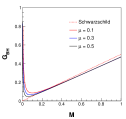
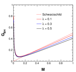
The variation of temperature of the black hole with mass $M$ for different values of the parameters of the theory as given by the expression (20) is shown in Fig. 1.

Figure 1: Variation of temperature of the black hole (11) with respect to mass for different values of $\alpha$, $\beta$, $\lambda$ and $\mu$ as obtained from Eq. (20). We use $\mu=\beta=\lambda=0.1$ for the first plot, $\mu=\alpha=\lambda=0.1$ for the second plot, $\mu=\alpha=\beta=0.1$ for the third plot and $\lambda=\alpha=\beta=0.1$ for the fourth plot respectively. The dotted line in each plot denotes the Schwarzschild case.

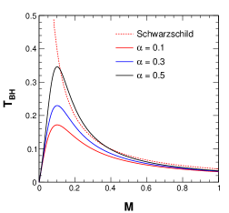
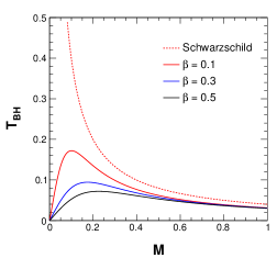
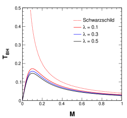
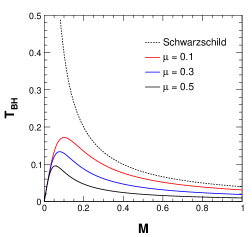
As seen in the plots, there is a little variation of temperature with change in the LSB parameter $\lambda$ (third plot). Whereas there is significant variations in temperature for the GUP parameters $\alpha$ and $\beta$, and the magnetic monopole parameter $\mu$. It is clear that with higher values of the GUP parameter $\alpha$, the peak value of temperature increases. The opposite situation can be seen for the other parameter $\beta$. The same decreasing behaviour is seen for $\mu$ and $\lambda$ as expected from the expression. It is to be noted that the temperature is positive, though it becomes smaller with increasing $M$. Moreover, for the small values of $M$, depending on the model parameter the value of temperature and its pattern are substantially different from the Schwarzschild case.

Next, we compute the heat capacity of the black hole from a relation obtained by using Eq. (16), considering $\mu$ as constant, given by

$$C_{BH}=\frac{dM_{K}}{dT}\Big{|}_{\mu}=T\,\frac{dS}{dT}.$$ (22)

This leads to the expression of heat capacity as

$$C_{BH}=-2\pi r_{H}^{2}=-\frac{\pi\Big{(}\beta(\mu-1)^{2}+8M^{2}+2\alpha(\mu-1)M\Big{)}^{2}}{8(\mu-1)^{2}M^{2}}.$$ (23)

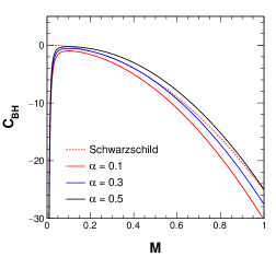
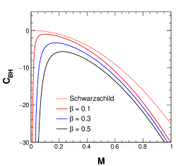
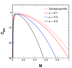
We plot the variations of $C_{BH}$ with respect to the black hole mass for different associated parameters of the model in Fig. 2. The first plot is for various values of $\alpha$, second one for $\beta$ and third one for $\mu$ . From the plots, it is observed that the heat capacity for the black hole always remains negative, signalling that the black hole is thermodynamically unstable. It can be seen that heat capacity is independent of LSB parameter $\lambda$. It is also clear from the plots of the figure that $C_{BH}$ decreases with increasing $M$ and as $M$ decreases towards zero, $C_{BH}$ becomes more and more negative, specifying the different behaviour of the black hole from the Schwarzschild one in this respect. The fact is that when a black hole emits more than it absorbs, then there is more probability of evaporation of the black hole, signifying instability.

It is to be noted that in this case, there is no possibility of remnant formation mathematically as clear from Eq. (23). The criteria for remnant formation states that $C_{BH}=0$ should be solved to find out the remnant radius, which when employed into the temperature expression (20), gives the remnant temperature 40 . The study of remnant formation is important in the sense that it provides an alternative to the theory of complete evaporation of the black hole. Once a remnant forms, it does not emit any radiation which may make it difficult to observe them directly.

Figure 2: Variation of heat capacity with respect to mass for different values of $\alpha$, $\beta$ and $\mu$. We use $\beta=\mu=0.1$ for the first plot, $\alpha=\mu=0.1$ for the second and $\alpha=\beta=0.1$ for the third plot respectively.

Entropy of a black hole is an important parameter that provides an idea about the information that falls into the black hole. Entropy is associated with the area of the black hole. As more and more matter falls into the black hole, the entropy of the black hole keeps on increasing and this is manifested by the increase in the horizon area of the black hole. The entropy of a black hole is related to the area of the horizon according to the relation,

$$S_{BH}\equiv\frac{A}{4}=\pi\,r_{H}^{2},$$ (24)

where $A$ denotes the area of the black hole. Alternatively, the entropy of a black hole can be calculated from the thermodynamic relation (16) as follows:

$$S_{BH}=\int\frac{dM_{K}}{T_{BH}},$$ (25)

which gives us the expression for the entropy of the black hole (11) as

$$S_{BH}=\pi r_{H}^{2}=\frac{\pi\Big{(}\beta(\mu-1)^{2}+8M^{2}+2\alpha(\mu-1)M\Big{)}^{2}}{16(\mu-1)^{2}M^{2}}.$$ (26)

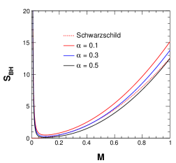
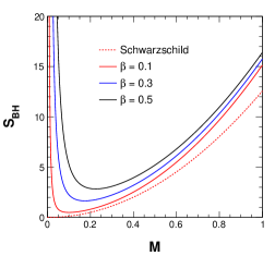
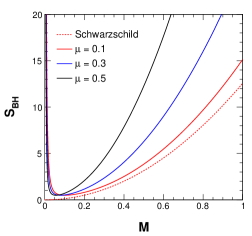
The equivalence of the two expressions (24) and (26) again confirms that the first law holds true. Fig. 3 shows the variation of entropy $S_{BH}$ with respect to the black hole mass for different values of the parameters of the theory. It is clear from the plots of this figure that entropy of this GUP-corrected black hole having topological defects increases with mass for all the cases. It is noted that similar to the heat capacity, entropy is also independent of $\lambda$. We note that the impacts of increasing $\alpha$ and $\beta$ are of reverse nature. For the monopole parameter $\mu$, we see that drastic increase of the entropy occurs with a larger value of $\mu$, as seen in the third plot. For mass approaching zero, entropy becomes highly positive.

Figure 3: Variation of entropy $S_{BH}$ with mass for various parameters of the theory. The first plot is for the variation of entropy for different values of $\alpha$, the second one for $\beta$ and the third plot is for different values of $\mu$. We use $\beta=\mu=0.1$ in the first plot, $\alpha=\mu=0.1$ in the second plot, and $\alpha=\beta=0.1$ in the third plot.

The Gibb’s free energy of a black hole is defined as 50

$$G_{BH}=M_{K}-T_{BH}S_{BH},$$ (27)

which gives the expression for the Gibb’s free energy for the black hole of our model as

$$G_{BH}=\frac{\beta(\mu-1)^{2}+8M^{2}+2\alpha(\mu-1)M}{16\sqrt{\lambda+1}M}.$$ (28)

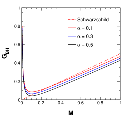
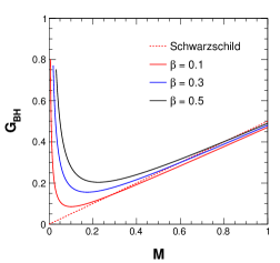
This expression is plotted with respect to mass $M$ for various parameters of the model in Fig. 4. As we can see from the plots, the variation of Gibbs free energy with mass is similar for $\alpha$, $\beta$, $\mu$ as well as $\lambda$. Larger values of parameters $\alpha$ and $\lambda$ induce a smaller rise in $G_{BH}$ with $M$. Whereas for $\beta$, this trend is opposite and for parameter $\mu$, the various graphs for different values of $\mu$ merge together as can be seen.

Figure 4: Variation of Gibbs free energy $G_{BH}$ with respect to mass $M$ for various parameters of the theory. The first plot is for the variation of $G_{BH}$ for different values of $\alpha$, the second one for different $\beta$ values, while the third plot is for different values of $\mu$ and fourth plot is for different values of $\lambda$. We use $\beta=\lambda=\mu=0.1$ in the first plot, $\alpha=\lambda=\mu=0.1$ in the second plot and $\alpha=\beta=\lambda=0.1$ in the third plot and $\alpha=\beta=\mu=0.1$ in the fourth plot.

In the following section, we study the shadow radius of the black hole as a function of various parameters of the theory. Then, in the next section, we derive an upper bound on the values of the various parameters of the theory by performing the classical test of precession of perihelion of planetary orbits. This kind of analysis was done earlier by Casana and his group 17 where they considered Schwarzschild-type metric with Lorentz violation parameter involved. Our work adds on the global monopole and GUP aspect to the study that provides us with interesting insights.

IV Shadow of the black hole

The shadow formed by a black hole depends on specific parameters of the theory and is specified by the photon sphere surrounding the black hole. In case of rotating black holes, the shadow is often distorted but when we consider spherically symmetric spacetimes, we generally encounter spherical shadow radius 1s . Here our aim is to study the shadow behaviour of the black hole in presence of the global monopole, LSB parameter and GUP correction. To start off, we form the geodesic equations of a photon moving in the black hole spacetime as follows.

The Lagrangian $\mathcal{L}(x,\dot{x})=\frac{1}{2}\,g_{\mu\nu}\dot{x}^{\mu}\dot{x}^{\nu}$ for the case of a spherically symmetric and static spacetime metric can be expressed as shnew02

$$\mathcal{L}(x,\dot{x})=\frac{1}{2}\left[-f(r)\,\dot{t}^{2}+\frac{1}{g(r)}\,\dot{r}^{2}+r^{2}\left(\dot{\theta}^{2}+\sin^{2}\theta\dot{\phi}^{2}\right)\right],$$ (29)

where the dot over the variable denotes the derivative with respect to the proper time $\tau$ and for our considered black hole spacetime metric (11), we have the following form of the metric functions:

$$f(r)=1-\mu-\frac{2M_{GUP}}{r}\;\;\;\text{and}\;\;\;g(r)=\frac{f(r)}{(1+\lambda)}.$$

We use the Euler-Lagrange equation: $\frac{d}{d\tau}\!\left(\frac{\partial\mathcal{L}}{\partial\dot{x}^{\mu}}\right)-\frac{\partial\mathcal{L}}{\partial x^{\mu}}=0$ and choose the equatorial plane, i.e. $\theta=\pi/2$, in order to derive the conserved quantities of the system, viz. energy and angular momentum. Two killing vectors $\partial/\partial\tau$ and $\partial/\partial\phi$ yield conserved energy $\mathcal{E}$ and angular momentum $L$ for the considered case as

$$\mathcal{E}=f(r)\,\dot{t},\quad L=r^{2}\dot{\phi}.$$ (30)

In case of photon, the geodesic equation leads to the relation,

$$-f(r)\,\dot{t}^{2}+\frac{(1+\lambda)}{f(r)}\,\dot{r}^{2}+r^{2}\dot{\phi}^{2}=0.$$ (31)

We utilise the conserved quantities i.e. $\mathcal{E}$ and $L$ in the above Eq. (31), which is required for obtaining the photon’s orbital equation as given by shnew01

$$\left(\frac{dr}{d\phi}\right)^{2}=\frac{r^{4}}{(1+\lambda)}\left[\frac{\mathcal{E}^{2}}{L^{2}}-\frac{f(r)}{r^{2}}\right].$$ (32)

Defining the right hand side of the above equation as an effective potential $V_{eff}$, i.e.

$$V_{eff}=\frac{r^{4}}{(1+\lambda)}\left[\frac{\mathcal{E}^{2}}{L^{2}}-\frac{f(r)}{r^{2}}\right]$$ (33)

the equation can be expressed in a compact form as

$$\left(\frac{dr}{d\phi}\right)^{2}=V_{eff}.$$ (34)

Moreover, Eq. (32) can be rewritten in the form of a radial equation as given by

$$\dot{r}^{2}+V_{r}(r)=\frac{\mathcal{E}^{2}}{1+\lambda},$$ (35)

where $V_{r}(r)$ is a new potential, we refer it as the reduced potential, which has the following form:

$$V_{r}(r)=\frac{f(r)L^{2}}{r^{2}(1+\lambda)}.$$ (36)

It is to be noted that since the angular momentum $L$ is a conserved quantity, it remains constant throughout and hence it will not have any impact on the overall behaviour of the reduced potential $V_{r}(r)$. Thus for the simplicity we will consider $L=1$ in our calculation of this potential. Further, as this potential governs the radial motion of photons in the black hole spacetime, the study of the behaviour of this potential with respect to the radial distance $r$ would be the realistic approach to understand the nature of the photon sphere around the black hole spacetime we have considered.

Figure 5: Variation of the reduced potential $V_{r}(r)$ with respect to distance $r$ as obtained by using $M=1$, $\alpha=0.8$, $\beta=0.05$, $\lambda=0.3$ and $\mu=0.2$.

Figure 6: Variation of the reduced potential $V_{r}(r)$ with respect to distance $r$ for different values of LSB parameter $\lambda$ (left plot) and global monopole term $\mu$ (right plot). We use $M=1$, $\alpha=0.1$, $\beta=0.05$ and $\mu=0.2$ in the left plot, and $M=1$, $\alpha=0.1$, $\beta=0.05$ and $\lambda=0.3$ in the right plot.

Figure 7: Variation of the reduced potential $V_{r}(r)$ with respect to distance $r$ for different values GUP parameters $\alpha$ (left plot) and $\beta$ (right plot). We use $M=1$, $\beta=0.05$, $\lambda=0.3$ and $\mu=0.2$ in the left plot, and $M=1$, $\alpha=0.1$, $\mu=0.2$ and $\lambda=0.3$ in the right plot.

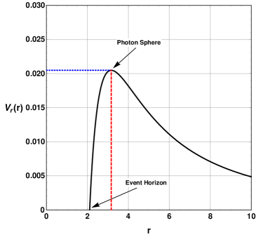
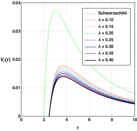
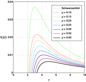
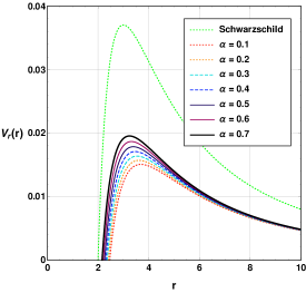
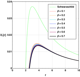
In Fig. 5 we show the behaviour of this reduced potential $V_{r}(r)$ with respect to distance $r$. In the figure the peak position of the potential curve represents the photon sphere, whose radius is measured as a parallel distance from the $y$-axis to peak position and is distinctly shown in the plot. On the left panel of Fig. 6 we show the behaviour of this potential with respect to $r$ for different values of LSB parameter $\lambda$. One can see that with an increase in the LSB parameter $\lambda$, the peak value of the potential decreases significantly. However, this parameter does not have any impact on the photon sphere size of the black hole as the peak position of the potential does not change its position with respect to $r$. On the right panel of Fig. 6 we plot the potential with respect to $r$ for different values of the global monopole term $\mu$. It shows that the global monopole parameter can have a significant impact on the potential as well as the photon sphere of the black hole. With an increase in the value of $\mu$, the peak value of the potential decreases drastically while the photon sphere size increases noticeably. In Fig. 7 we show the behaviour of the potential for different values of the GUP parameters. On the left panel we consider different values of the first GUP parameter $\alpha$, where we have seen that with an increase in value of $\alpha$, the peak value of the potential increases, unlike the scenario for the LSB parameter $\lambda$ and monopole parameter $\mu$. The photon sphere size decreases with an increase in the value of $\alpha$. On the right panel of Fig. 7, we show the impacts of the second GUP parameter $\beta$ on the potential of the black hole. Here, we see that with an increase in the value of the parameter $\beta$, the photon sphere increases in size while the peak value of the potential decreases. From this graphical analysis we have seen that the size of the photon sphere basically depends on three parameters only, viz., monopole term $\mu$, GUP parameters $\alpha$ and $\beta$. The second GUP parameter $\beta$ has the smallest impact on the potential of the black hole, as seen from the analysis.

Now, we move to the analysis of the shadow of the black hole. To obtain the shadow of the black hole, we consider the trajectory’s turning point, denoted by $r=r_{ph}$, which is in fact the radius of the photon sphere or light ring around the black hole. At this turning point, the conditions that must be satisfied are 18 ; synge ; Luminet:1979nyg

$$\left.\frac{dr}{d\phi}\right|_{r_{ph}}\!\!\!\!\!\!\!=0\;\;\text{or}\;\;\left.V_{eff}\right|_{r_{ph}}\!\!\!\!=0,\;\;\text{and}\;\;\;\left.\frac{d^{2}r}{d\phi^{2}}\right|_{r_{ph}}\!\!\!\!\!\!\!=0\;\;\text{or}\;\;\left.V_{eff}^{\prime}\right|_{r_{ph}}\!\!\!\!=0.$$ (37)

The impact parameter $b$ at the turning point obtained from the first condition is

$$\frac{1}{b_{crit}^{2}}=\frac{f(r_{ph})}{r_{ph}^{2}}.$$ (38)

Here, the parameter $b$ is defined as $b=L/\mathcal{E}$. From the second one of above conditions one can find the radius of the photon sphere $r_{ph}$ by solving the equation:

$$\left.\frac{d}{dr}\,\mathcal{A}(r)\right|_{r_{ph}}\!\!\!\!\!\!\!=0,$$ (39)

which can be written explicitly as

$$\frac{f^{\prime}(r_{ph})}{f(r_{ph})}-\frac{h^{\prime}(r_{ph})}{h(r_{ph})}=0,$$ (40)

where $\mathcal{A}(r)=h(r)/f(r)$ with $h(r)=r^{2}$. The analysis of Eqs. (38) and (40) shows that the radius of the photon sphere is at $r_{ph}=3M_{GUP}/(1-\mu)$ and the critical impact parameter is $b_{crit}=3\sqrt{3}M_{GUP}/\sqrt{1-\mu^{3}+3\mu^{2}-3\mu}$. In the absence of the GUP corrections and global monopole, the radius of the photon sphere is $r_{ph}=3M$ and the critical impact parameter is $b_{crit}=3\sqrt{3}M$ which corresponds to a Schwarzschild black hole.

In terms of the function $\mathcal{A}(r)$, Eq. (32) can be rewritten with Eq. (38) as

$$\left(\frac{dr}{d\phi}\right)^{\!2}=\frac{h(r)f(r)}{1+\lambda}\left(\frac{\mathcal{A}(r)}{\mathcal{A}(r_{ph})}-1\right).$$ (41)

This equation can be used to calculate the shadow radius. For this purpose, if we consider that $\alpha$ is the angle between the light rays from a static observer at $r_{0}$ and the radial direction of the photon sphere, then the angle $\alpha$ can be found as Perlick:2021aok ; 18

$$\cot\alpha=\frac{\sqrt{(1+\lambda)}}{\sqrt{f(r)h(r)}}\left.\frac{dr}{d\phi}\right|_{r\,=\,r_{0}}\!\!\!\!\!\!\!\!\!\!\!.$$ (42)

With Eq. (41), above equation can be expressed as

$$\cot^{2}\!\alpha=\frac{\mathcal{A}(r_{0})}{\mathcal{A}(r_{ph})}-1.$$ (43)

Using the relation $\sin^{2}\!\alpha=1/(1+\cot^{2}\!\alpha)$, above equation can be rewritten as

$$\sin^{2}\!\alpha=\frac{\mathcal{A}(r_{ph})}{\mathcal{A}(r_{0})}.$$ (44)

Substituting the actual form of $\mathcal{A}(r_{ph})$ from Eq. (38) and $\mathcal{A}(r_{0})=r_{0}^{2}/f(r_{0})$, the shadow radius of the black hole for a static observer at $r_{0}$ is found as 15s

$$R_{s}=r_{0}\sin\alpha=\sqrt{\frac{r_{ph}^{2}f(r_{0})}{f\left(r_{ph}\right)}}.$$ (45)

Again, for a static observer at large distance, i.e. at $r_{0}\rightarrow\infty$, $f(r_{0})\rightarrow 1$, so for such an observer the shadow radius $R_{s}$ becomes,

$$R_{s}=\frac{r_{ph}}{\sqrt{f(r_{ph})}}.$$ (46)

Finally, the apparent shape of the shadow can be found by the stereographic projection of the shadow from the black hole’s plane to the observer’s image plane with coordinates $(X,Y)$. These coordinates are defined as shnew03

$$X =\lim_{r_{0}\rightarrow\infty}\left(-\,r_{0}^{2}\sin\theta_{0}\left.\frac{d\phi}{dr}\right|_{r_{0}}\right),$$ (47)

$$Y =\lim_{r_{0}\rightarrow\infty}\left(r_{0}^{2}\left.\frac{d\theta}{dr}\right|_{(r_{0},\theta_{0})}\right),$$ (48)

where $\theta_{0}$ is angular position of the observer with respect to the black hole’s plane.

Figure 8: Stereographic projection of the black hole shadow in the observer image plane obtained by using (a) $\alpha=0.1$, $\beta=0.01$ and $\mu=0.1$ on the left panel and (b) $\alpha=0.1$, $\beta=0.01$ and $M=1$ on the right panel.

Figure 9: Stereographic projection of the black hole shadow in the observer image plane obtained by using (a) $M=1$, $\beta=0.01$ and $\mu=0.1$ on the left panel and (b) $M=1$, $\alpha=0.1$ and $\mu=0.1$ on the right panel.

Figure 10: Variation of $\frac{1}{R_{s}}$ with respect to $\mu$ for $M=1$. On the left panel we use $\beta=0.1$ and on the right panel we use $\alpha=0.1$.

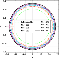
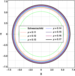
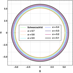
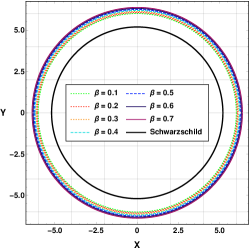
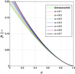
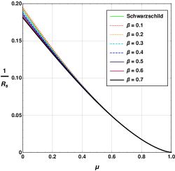
In Fig. 8, on the left panel, we show the stereographic projection of the shadow of the black hole for different values of the black hole mass $M$. As usual, with an increase in the mass, the shadow radius of the black hole increases. On the right panel, we show the shadow of the black hole for different values of the monopole parameter $\mu$. It is seen that with an increase in the value of $\mu$, the shadow radius increases in agreement with the earlier observation from Fig. 6 of the black hole potential. Fig. 9 shows the shadow of the black hole for different values of the GUP parameters $\alpha$ and $\beta$. As evident from the analysis of the black hole potential, both parameters have opposite impacts on the black hole shadow. When $\alpha$ increases, the shadow size decreases gradually. However, the impact of $\alpha$ is smaller and opposite compared to $\mu$. The other GUP parameter $\beta$ has the smallest impact on the size of the black hole shadow as seen from the graph on the right panel of Fig. 9. With an increase in the parameter $\beta$, the shadow radius of the black hole increases slowly. To have a more clear visualisation, we plot the inverse of the black hole shadow radius with respect to the global monopole parameter $\mu$ for different values of the GUP parameters in Fig. 10. On the left panel of Fig. 10, we consider different values of $\alpha$. One can see that $\frac{1}{R_{s}}$ increases with an increase in the values of $\alpha$ for smaller values of $\mu$. However, for large values of $\mu$, the GUP parameter has negligible impacts on the inverse of the black hole shadow radius. From the right panel of Fig. 10, it is seen that the inverse of the shadow radius decreases for smaller values of $\mu$. Again for higher values of $\mu$, the impact of GUP parameter $\beta$ is negligible.

V A Classical test: Advancement of the perihelion of planets

The geodesic equation for the motion of a test particle along a path described by the four-coordinate $x^{\mu}(\tau)$ is given by

$$\frac{d^{2}x^{\mu}}{d\tau^{2}}+\Gamma^{\mu}_{\sigma\nu}\frac{dx^{\sigma}}{d\tau}\frac{dx^{\nu}}{d\tau}=0,$$ (49)

where $\tau$ is the affine parameter. We consider a constant of motion $\chi$ associated with the geodesic, which is defined as

$$\chi=-\,g_{\mu\nu}U^{\mu}U^{\nu},$$ (50)

where the vector $U^{\mu}$ is of the form:

$$U^{\mu}=\frac{dx^{\mu}}{d\tau}=\dot{x^{\mu}}.$$ (51)

Here, the differentiation with respect to $\tau$ parameter is represented by dot over the variable. For massive particles, $\chi=1$ and for massless particles, $\chi=0.$ Using Eq. (49), the massless particle’s trajectory in the spacetime (11) can be stated in the form of the following equations:

$$\ddot{t}-\frac{A}{2r\Big{(}A-4Mr(1-\mu)\Big{)}}\,\dot{r}\,\dot{t} =0,$$ (52)

$$\ddot{r}+\frac{A}{2r(A-4Mr(1-\mu))}\,\dot{r}^{2}-\frac{A\Big{(}A-4Mr(1-\mu)\Big{)}}{32\,M^{2}r^{3}(1+\lambda)}\,\dot{t}^{2}$$

$$+\,\frac{A}{4M(1+\lambda)}\,\dot{\theta}^{2}+\frac{A-4Mr(1-\mu)}{4M(1+\lambda)}\,\sin^{2}\theta\,\dot{\phi}^{2} =0,$$ (53)

$$\ddot{\theta}+\frac{2}{r}\,\dot{r}\,\dot{\theta}-\cos\theta\sin\theta\,\dot{\phi}^{2} =0,$$ (54)

$$\ddot{\phi}+\frac{2}{r}\,\dot{r}\,\dot{\phi}+2\cot\theta\,\dot{\theta}\,\dot{\phi} =0,$$ (55)

where $A=8M^{2}-2M\alpha(1-\mu)+\beta(1-\mu)^{2}$. It is to be noted that the affine parameter $\tau$ is chosen to be the proper time in case of massive test particles and the initial conditions are $\theta(\tau_{0})=\frac{\pi}{2}$ and $\dot{\theta}(\tau_{0})=0$. From Eq. (50), for the massive test particle in timelike geodesic, we have the following differential equation for the coordinate $r$:

$$(1+\lambda)\,\dot{r}^{2}+\Big{(}1+\frac{L^{2}}{r^{2}}\Big{)}\Big{[}1-\mu-\frac{2M}{r}\Big{(}1-\frac{\alpha(1-\mu)}{4M}+\frac{\beta(1-\mu)^{2}}{8M^{2}}\Big{)}\Big{]}=E^{2}.$$ (56)

Following Ref. 17 , we introduce a new variable $m=r^{-1}$ such that we have

$$\dot{r}=-\,L\,\frac{dm}{d\phi}.$$ (57)

By using Eq. (57) in Eq. (56), we can write

$$m^{2}(1-\mu)+(1+\lambda)\left(\frac{dm}{d\phi}\right)^{2}=\frac{E^{2}-(1-\mu)}{L^{2}}+2Mm\left(\frac{1}{L^{2}}+m^{2}\right)\bigg{[}1-\frac{\alpha(1-\mu)}{4M}+\frac{\beta(1-\mu)^{2}}{8M^{2}}\bigg{]}.$$ (58)

Taking the derivative of this Eq. (58) with respect to $\phi$, we obtain

$$(1+\lambda)\,\frac{d^{2}m}{d\phi^{2}}+m(1-\mu)-\bigg{(}\frac{M}{L^{2}}+3\,m^{2}M\bigg{)}\bigg{[}1-\frac{\alpha(1-\mu)}{4M}+\frac{\beta(1-\mu)^{2}}{8M^{2}}\bigg{]}=0.$$ (59)

The above differential equation in one variable contains contributions of both Lorentz symmetry violation parameter and global monopole term. In order to solve this type of equation, we use the perturbative method, for which define the variable $m$ as

$$m=m^{(0)}+\epsilon\,m^{(1)},$$ (60)

where the small perturbative parameter $\epsilon=\frac{3M^{2}}{L^{2}}$ and $\epsilon<<1$ 17 . Using this, the Eq. (59) for the zeroth order in $\epsilon$ gives

$$(1+\lambda)\frac{d^{2}m^{(0)}}{d\phi^{2}}+m^{(0)}(1-\mu)-\frac{M}{L^{2}}\bigg{[}1-\frac{\alpha(1-\mu)}{4M}+\frac{\beta(1-\mu)^{2}}{8M^{2}}\bigg{]}=0.$$ (61)

Solution of this differential Eq. (61) for zeroth order in $\epsilon$ gives

$$m^{(0)}=\frac{M_{GUP}}{(1-\mu)L^{2}}\bigg{[}1+e\cos\frac{\phi\sqrt{1-\mu}}{\sqrt{1+\lambda}}\bigg{]}.$$ (62)

It is to be noted that when we substitute $\alpha=\beta=\mu=0$ in the above Eq. (62), we get back the expected GR result. Here $e$ is the eccentricity of the orbit. We then implement the differential Eq. (59) for the variable in Eq. (60) to the first order in $\epsilon$ to get the differential equation as

$$(1+\lambda)\frac{d^{2}m^{(1)}}{d\phi^{2}}+m^{(1)}(1-\mu)-\frac{L^{2}m^{(0)2}}{M_{GUP}}=0.$$ (63)

Solutions of the two differential Eqs. (61) and (63) when clubbed in Eq. (60) gives an ellipse-like equation after the small $\epsilon$ approximation as

$$m=\frac{M_{GUP}}{(1-\mu)L^{2}}\bigg{[}1+e\Big{(}\cos\frac{\sqrt{1-\mu}}{\sqrt{1+\lambda}}\phi(1-\epsilon)\Big{)}\bigg{]}.$$ (64)

Eq. (64) represents the perturbative solution of the original differential Eq. (59). It is quite clear from the expression of period that the GUP parameters play no role regarding the precession of orbits. Despite the presence of different factors of model considered in the study, the orbit is periodic as can be seen from the expression with a period,

$$\Phi=\frac{2\pi\sqrt{1+\lambda}}{\sqrt{1-\mu}(1-\epsilon)}=2\pi+\Delta\Phi.$$ (65)

The quantity $\Delta\Phi$ represents the advance of the perihelion of the massive object (planet) which is expressed by expanding the above expression in lowest order of $\epsilon$, $\lambda$ and $\mu$ as

$$\Delta\Phi=2\pi\epsilon+\pi\lambda+\pi\mu+\frac{\pi\lambda\mu}{2}=\Delta\Phi_{GR}+\Delta\Phi_{LV}+\Delta\Phi_{GM}+\Delta\Phi_{LVGM}.$$ (66)

Here, $\Delta\Phi_{GR}$, $\Delta\Phi_{LV}$, $\Delta\Phi_{GM}$ and $\Delta\Phi_{LVGM}$ means usual GR contribution, contribution due to Lorentz violation, contribution due to global monopole term, and a mixed contribution from both the Lorentz violation and global monopole respectively. It is clear that along with $2\pi\epsilon$ term which appears in GR, we have some extra contributions to the period of the orbit.

The perihelion precession data of various planets and an asteroid Icarus whose time periods of revolution around the sun in elliptical orbits are known from various experimental observations 17 . The uncertainty associated with these precession data is thus available which is assumed to be the upper bounds of any deviation from GR. But the issue which we now face is that there are two quantities $\lambda$ and $\mu$ in our case, which makes the exact determination hard from one single constraint equation. Thus we can estimate that the product of these two quantities is less than this bound as will be clear from the table 1 below as well as from Eq. (66).

Here we present a tabular data of precession of some inner planets and an asteroid in units of arc-seconds per century and compare the GR-predicted and observed values and also present an estimate of the upper bounds on the parameters $\lambda$ and $\mu$. Stringent upper bounds are obtained from the precession data of Earth and Mars of the order of $10^{-12}$, while for the asteroid Icarus, the upper bound obtained is of the order $10^{-8}$ only.

Table 1: The precession data, the orbital periods and upper bounds of model parameters for some planets and the asteroid Icarus 17 ; 57 ; 58 ; 59 ; 60 ; 61 . Precession data is in the unit of arc-second per century.

Planet/Asteroid	Predicted by GR	Observation with error	Orbital period (in days)	Upper Bounds for $(\lambda+\mu+\frac{\lambda\mu}{2})$
Mercury	$42.981$	$42.981\pm 0.0030$	$88.0$	$1.1\times 10^{-11}$
Venus	$8.6247$	$8.6273\pm 0.0016$	$224.7$	$1.5\times 10^{-11}$
Earth	$3.83877$	$3.83896\pm 0.00019$	$365.2$	$2.9\times 10^{-12}$
Mars	$1.350938$	$1.350918\pm 0.000037$	$687.0$	$1.1\times 10^{-12}$
Icarus (asteroid)	$10.10$	$9.80\pm 0.80$	$409.0$	$1.3\times 10^{-8}$

It is to be noted that the bounds are similar to the ones obtained in 17 , where the authors employed the LSB only. However, we obtained additional bounds on $\mu$, the global monopole parameter and the product of $\mu$ an $\lambda$ as shown in the table 1. Another point that has to be mentioned is that the perihelion precession test of planetary orbits is very well explained by GR theory and thus very small deviations in the form of errors are seen. This is the reason for the very minute values of the parameters obtained as bounds.

VI Conclusion

In this work we have studied the various thermodynamic relations and shadows for a spherically symmetric and static GUP-corrected Schwarzschild-type black hole solution which contains the topological defects and Lorentz symmetry violation in Bumblebee gravity, presented in the Ref. 20 . The black hole temperature variation with respect to black hole mass for various parameters of the model was almost identical in the sense that initially the temperature increases to a peak and then it decreases continuously with increase in the mass of the black hole. It may be highlighted that as the black hole increases in mass, its temperature gradually decreases and approaches zero. But it does not turn negative and hence there is no possibility of the formation of an ultracold black hole 62 . Thermodynamically stable black holes have positive heat capacity and the one we studied did not show this property. We studied the variation of heat capacity with various parameters of our theory. It is to be noted that when a black hole absorbs more energy than it is throwing out, its mass will increase indefinitely, whereas when it emits more than it absorbs, then it will eventually disappear. Such is the situation with negative heat capacities, wherein emission is more than absorption, causing instability. In this regard, our black hole spacetime shows instability similar to Schwarzschild case. We study the entropy function and its variation with respect to mass for various values of our model parameters. It was found that entropy increases with mass for all the cases. Gibbs free energy variations have been studied and we see similar a increasing trend in variation for all four model parameters.

We studied the shadow radius for the black hole with variations of different parameters of the theory. The shadow of the black hole is a suitable optical characteristic which plays a significant role from the observational perspective. Our investigation shows that the presence of the global monopole has a significant impact on the shadow radius of the black hole. An interesting fact is that when the global monopole parameter increases, the effects of the GUP parameters become negligible. It basically implies that it might be challenging to probe the quantum corrections like GUP corrections associated with a black hole in presence of a global monopole in spacetime by utilising the shadow analysis of the black hole. Another result obtained here is that the global monopole and the second GUP parameter $\beta$ have similar impacts on the black hole shadow. Although the peak of the reduced potential of the black hole is significantly affected by the Lorentz symmetry breaking, one may note that photon sphere position is independent of the Lorentz symmetry violation. As a result, we do not have any impacts on the shadow radius by the Lorentz symmetry violation. In recent years, the Event Horizon Telescope (EHT) has made significant strides in its efforts to capture an ultra-high resolution image of the accretion flows surrounding a supermassive black hole in the galaxy M87^∗. These efforts have finally culminated in the acquisition of a groundbreaking image that showcases the inner workings of the black hole’s accretion process 6 ; 7 ; 8 ; 9 ; 10 ; 11 .

The first image of M87^∗ reveals a strikingly bright ring encircling the black hole’s dark interior. This ring, known as the photon ring, serves as a critical observation feature of the black hole. Meanwhile, the black hole’s dark center, known as its shadow, is prominently displayed in the image. These observations are groundbreaking in their ability to shed light on the mysterious nature of supermassive black holes and the processes that govern their behavior. An extension of this current work may be constraining the shadow radius using the observational results. In view of observational data related to shadow radius made available by EHT recently, it is possible to put constraints on various parameters like GUP and the monopole parameter. This remains as a future extension of our work.

We did a classical test of GR also, namely the perihelion precession of inner planets and an asteroid. It is seen that the GUP parameters do not contribute towards the period of precession of the planetary orbits. Moreover, the upper bounds obtained are not very stringent as number of parameters is two in our case. It can be concluded that this method of constraining the parameters works best when we work with one parameter as in case of 17 . Various other tests like bending of light and Shapiro time delay of light have been used to constrain the parameters of the theory, which we have not dealt with now and keep it as a future scope of study.

References

- (1) B. P. Abbott et al., Observation of Gravitational Waves from a Binary Black Hole Merger, Phys. Rev. Lett. 116, 061102 (2016).
- (2) B. P. Abbott et al., Observation of Gravitational Waves from a 22-Solar-Mass Binary Black Hole Coalescence, Phys. Rev. Lett. 116, 241103 (2016).
- (3) B. P. Abbott et al., Observation of Gravitational Waves from a Binary Neutron Star Inspiral, Phys. Rev. Lett. 119, 161101 (2017).
- (4) B. P. Abbott et al., Observation of a Binary-Black-Hole Coalescence with Asymmetric Masses, Phys. Rev. D 102, 043015 (2020).
- (5) R. Abbott et al., Observation of Gravitational Waves from Two Neutron Star–Black Hole Coalescences, ApJL 915, L5 (2021).
- (6) The Event Horizon Telescope Collaboration et al., First M87 Event Horizon telescope Results. I. The Shadow of the supermassive Black Hole, ApJL 875, L1 (2019).
- (7) The Event Horizon Telescope Collaboration et al., First M87 Event Horizon telescope Results. II. Array and Instrumentation, ApJL 875, L2 (2019).
- (8) The Event Horizon Telescope Collaboration et al., First M87 Event Horizon telescope Results. III. Data Processing and Calibration, ApJL 875, L3 (2019).
- (9) The Event Horizon Telescope Collaboration et al., First M87 Event Horizon telescope Results. IV. Image the Central Supermassive Black Hole, ApJL 875, L4 (2019).
- (10) The Event Horizon Telescope Collaboration et al., First M87 Event Horizon telescope Results. V. Physical Origin of the Asymmetric Ring, ApJL 875, L5 (2019).
- (11) The Event Horizon Telescope Collaboration et al., First M87 Event Horizon telescope Results. VI. The Shadow and Mass of the Central Black Hole, ApJL 875, L6 (2019).
- (12) A. G. Riess et al., Observational Evidence from Supernovae for an Accelerating Universe and a Cosmological Constant, The Astronomical Journal 116, 1009 (1998).
- (13) S. Perlmutter et al., Measurements of and from 42 High-Redshift Supernovae, ApJ 517, 565 (1999).
- (14) K. S. Stelle, Renormalization of Higher-Derivative Quantum Gravity, Phys. Rev. D 16, 953 (1977).
- (15) C. Pérez de los Heros, Status, Challenges and Directions in Indirect Dark Matter Searches, Symmetry 12, 1648 (2020).
- (16) N. A. Bahcall, The Cosmic Triangle: Revealing the State of the Universe, Science 284, 1481 (1999).
- (17) Fundamental decoherence from quantum gravity: a pedagogical review, Gen. Relativ. Gravit. 39, 1143 (2007).
- (18) G. Amelino-Camelia, Are We at the Dawn of Quantum-Gravity Phenomenology?, Towards Quantum Gravity. Lecture Notes in Physics, vol 541. Springer, Berlin, Heidelberg (2000).
- (19) C. Rovelli, Loop Quantum Gravity, Living Reviews in Relativity 11, 5 (2008).
- (20) A. Asthekar and E. Bianchi, A short review of loop quantum gravity, Reports on Progress in Physics 84, 042001 (2021).
- (21) Í. Güllü and A. Övgün, Schwarzschild-like black hole with a topological defect in bumblebee gravity, Annals of Physics 436, 168721 (2022).
- (22) D. J. Gogoi and U. D. Goswami, Quasinormal Modes and Hawking Radiation Sparsity of GUP corrected Black Holes in Bumblebee Gravity with Topological Defects, JCAP 06, 029 (2022).
- (23) R. Casana, A. Cavalcante, F. P. Poulis and E. B. Santos, Exact Schwrzschild-like solution in a bumblebee gravity model, Phys. Rev. D 97, 104001 (2018).
- (24) R. Oliveira, D. M. Dantas and C. A. S. Almeida, Quasinormal frequencies for a black hole in a bumblebee gravity, Europhysics Lett. 135, 1 (2021).
- (25) M. Khodadi and M. Schreck, Hubble tension as a guide for refining the early Universe: Cosmologies with explicit local Lorentz and diffeomorphism violation, Physics of the Dark Universe 39, 101170 (2023).
- (26) M. Khodadi, G. Lambiase and L. Mastrototaro, Spontaneous Lorentz symmetry breaking effects on GRBs jets arising from neutrino pair annihilation process near a black hole, EPJC 83, 239 (2023).
- (27) M. Khodadi, G. Lambiase and A. Sheykhi, Constraining the Lorentz-Violating Bumblebee Vector Field with Big Bang Nucleosynthesis and Gravitational Baryogenesis, arXiv:2211.07934 [gr-qc] (2022).
- (28) M. Khodadi, Black hole superradiance in the presence of Lorentz symmetry violation, Phys. Rev. D 103, 064051 92021).
- (29) T. P. Sotiriou and V. Faraoni, f(R) theories of gravity, Rev. Mod. Phys. 82, 451 (2010).
- (30) A. De Felice and S. Tsujikawa, f(R) Theories, Living Reviews in Relativity 13, 3 (2010).
- (31) D. J. Gogoi and U. D. Goswami, A new f(R) gravity model and properties of gravitational waves in it, EPJC 80, 1101 (2020).
- (32) T. Harko, F. S. N. Lobo, S. Nojiri and S. D. Odintsov, f(R,T) gravity, Phys. Rev. D 84, 024020 (2011).
- (33) P. Rastall, Generalization of the Einstein Theory, Phys. Rev. D 6, 3357 (1972).
- (34) S. Bahamonde et. al., Teleparallel gravity: from theory to cosmology, Reports on Progress in Physics 86, 026901 (2023).
- (35) R. Maartens and K. Koyama, Brane-World Gravity, Living Rev. Relativ 13, 5 (2010).
- (36) A. De and L. How, ”Comments on Energy conditions in f(Q) gravity”, Phys. Rev. D 106, 048501 (2022).
- (37) R. Bluhm, Overview of the Standard Model Extension: Implications and Phenomenology of Lorentz Violation, Lecture Notes in Physics, vol 702. Springer, Berlin, Heidelberg (2006).
- (38) D. Colladay and V. A. Kostelecky, CPT violation and the standard model, Phys. Rev. D 55, 6760 (1997).
- (39) T. Harko, Galactic Rotation curves in modified gravity with nonminimal coupling between matter and geometry, Phys. Rev. D 81, 084050 (2010).
- (40) A. Vilenkin, Cosmological evolution of monopoles connected by strings, Nuclear Phys. B 196,240 (1982).
- (41) U. D. Goswami, Supersymmetric hybrid inflation with non-minimal coupling to gravity, Eur. Phys. J. Plus 135, 44 (2020).
- (42) S. Das and E. C. Vagenas, Universality of Quantum Gravity Corrections, Phys. Rev. Lett. 101, 221301 (2008).
- (43) A. F. Ali, S. Das and E. C. Vagenas, Discreteness of space from the generalized uncertainty principle, Phys. Lett. B 678, 497 (2009).
- (44) S. Das and E. C. Vagenas, Phenomenological Implications of the Generalized Uncertainty Principle, Can. J. Phys. 87, 1139 (2009).
- (45) S. Das and E. C. Vagenas, Reply to ”Comment on ’Universality of Quantum Gravity Corrections’”, Phys. Rev. Lett 104, 119002 (2010).
- (46) A. F. Ali, S. Das and E. C. Vagenas, The Generalized Uncertainty Principle and Quantum Gravity Phenomenology, The Twelfth Marcel Grossmann Meeting, pp. 2407-2409 (2012).
- (47) S. Das, E. C. Vagenas and A. F. Ali, Discreteness of space from GUP II: Relativistic wave equations, Phys. Lett. B 690, 407 (2010).
- (48) N. Heidari, H. Hassanabadi and H. Chen, Quantum-corrected scattering of a Schwarzschild black hole with GUP effect, Phys. Lett. B 838, 137707 (2023).
- (49) M. A. Anecleto, F. A. Brito, J. A. V. Campos and E. Passos, Quasinormal modes and shadow of a Schwarzschild black hole with GUP, Annals of Physics 434, 168662 (2021).
- (50) B. Hamil, B. C. Lütfüoglu, and L. Dahbi, EUP-corrected thermodynamics of BTZ black hole, Int. J. Mod. Phys. A 37 2250130 (2022).
- (51) M. A. Anecleto, F. A. Brito, J. A. V. Campos and E. Passos, Quantum-corrected scattering and absorption of a Schwarzschild black hole with GUP, Phys. Lett. B 810, 135830 (2020).
- (52) B. C. Lütfüoglu, B. Hamil and L. Dahbi, Thermodynamics of Schwarzschild black hole surrounded by quintessence with generalized uncertainty principle, EPJP 136, 976 (2021).
- (53) S. Hossenfelder, Minimal Length Scale Scenarios for Quantum Gravity, Living Reviews in Relativity 16, 2 (2013).
- (54) A. N. Tawfik, H. Magdy and A. F. Ali, Lorentz invariance violation and generalized uncertainty principle, Physics of Particles and Nuclei Letters 13, 59 (2016).
- (55) M. Khodadi, K. Nozari and E. N. Saridakis, Emergent universe in theories with natural UV cutoffs, Class. Quantum. Grav. 35, 015010 (2017).
- (56) M. Khodadi, K. Nozari and A. Hajizadeh, Some astrophysical aspects of a Schwarzschild geometry equipped with a minimal measurable length, Phys. Lett. B 770, 556 (2017).
- (57) M. Khodadi, K. Nozari, A. Bhat and S. Mohsenian, Probing Planck-scale spacetime by cavity opto-atomic 87Rb interferometry, Progress of Theoretical and Experimental Physics 2019, 053E03 (2019).
- (58) M. Khodadi, K. Nozari, H. Abedi and S. Capozziello, Planck scale effects on the stochastic gravitational wave background generated from cosmological hadronization transition: A qualitative study, Phys. Lett. B 783, 326 (2018).
- (59) M. Khodadi, K. Nozari and F. Hajkarim, On the viability of Planck scale cosmology with quartessence, EPJC 78, 716 (2018).
- (60) E. C. Vagenas, A. F. Ali, M. Hemeda and H. Alshal, Linear and quadratic GUP, Liouville theorem, cosmological constant, and Brick Wall entropy, EPJC 79, 398 (2019).
- (61) O. Okcu and E. Aydiner, Observational tests of the generalized uncertainty principle: Shapiro time delay, gravitational redshift, and geodetic precession, Nuclear Phys. B 964, 115324 (2021).
- (62) A. F. Ali, I. Elmashad and J. Mureika, Universality of minimal length, Phys. Lett. B 831, 137182 (2022).
- (63) K. Nozari and M. Hajebrahimi, Geodesic structure of the quantum-corrected Schwarzschild black hole surrounded by quintessence, IJGMMP 19, 2250177 (2022).
- (64) K. Nozari, M. Hajebrahimi and S. Saghafi, Quantum corrections to the accretion onto a Schwarzschild black hole in the background of quintessence, EPJC 80, 1208 (2020).
- (65) F. Scardigli, Generalized uncertainty principle in quantum gravity from micro-black hole gedanken experiment, Phys. Lett. B 452, 39 (1999).
- (66) F. Scardigli, M. Blasone, G. Luciano and R. Casadio, Modified Unruh effect from generalized uncertainty principle, EPJC 78, 728 (2018).
- (67) S. Segreto and G. Montani, Extended GUP formulation with and without truncation in momentum space, arXiv.2208.03101 (2022).
- (68) Z. W. Feng, H. L. Li, X. T. Zu and S. Z. Yang, Quantum corrections to the thermodynamics of Schwarzschild–Tangherlini black hole and the generalized uncertainty principle, EPJC 76, 212 (2016).
- (69) G. Lambiase, R. C. Pantig, D. J. Gogoi and A. Övgün, Investigating the Connection between Generalized Uncertainty Principle and Asymptotically Safe Gravity in Black Hole Signatures through Shadow and Quasinormal Modes, [arXiv:2304.00183](2023).
- (70) F. Atamurotov, I. Hussain, G. Mustafa and K. Jusufi, Shadow and quasinormal modes of the Kerr–Newman–Kiselev–Letelier black hole, EPJC 82, 831 (2022).
- (71) S. W. Hawking, Particle creation by black holes, Commun. Math. 43, 199 (1975).
- (72) J. M. Bardeen, B. Carter and S. W. Hawking, The four laws of black hole mechanics, Commun. Math 31, 161 (1973).
- (73) S. W. Hawking and D. N. Page, Thermodynamics of black holes in anti-de Sitter space, Commun. Math. 87, 577 (1983).
- (74) J. D. Bekenstein, Black Holes and Entropy, Phys. Rev. D 7, 2333 (1973).
- (75) J. D. Bekenstein, Generalized second law of thermodynamics in black-hole physics, Phys. Rev. D 9, 3292 (1974).
- (76) J. D. Bekenstein, Black Holes and the Second Law, Lettere al Nuovo Cimento 4, 737 (1972).
- (77) M. Astorino, Thermodynamics of regular accelerating black holes, Phys. Rev. D 95, 064007 (2017).
- (78) C. H. Bayraktar, Thermodynamics of regular black holes with cosmic strings, Eur. Phys. J. C133, 377 (2018).
- (79) M. Dehghani, Thermodynamics of novel charged dilaton black holes in gravity’s rainbow, Phys. Lett. B 785, 274 (2018).
- (80) Y. Yao, M. -S. Hou and Y. C. Ong, A complementary third law for black hole thermodynamics, Eur. Phys. J. C 79, 513 (2019).
- (81) C. H. Bayraktar, Thermodynamics of regular black holes with cosmic strings, Eur. Phys. J. C133, 377 (2018).
- (82) M. Sharif and H. S. Nawaz, Thermodynamics of rotating regular black holes, Chin. Phys. C 67, 193 (2020).
- (83) M. Fathi, M. Molina and J. R. Villanueva, Adiabatic evolution of Hayward black hole, Phys. Lett. B 820, 136548 (2021).
- (84) M. Faizal and M. M. Khalil, GUP-corrected thermodynamics for all black objects and the existence of remnants, Int. J. Mod. Phys A 30 1550144 (2015).
- (85) R. Karmakar, D. J. Gogoi and U. D. Goswami, Quasinormal modes and thermodynamic properties of GUP-corrected Schwarzschild black hole surrounded by quintessence, IJMP A 37, 28 (2022).
- (86) Md. Shahjalal, Thermodynamics of quantum-corrected Schwarzschild black hole surrounded by quintessence, Nucl. Phys. B 940, 63 (2019).
- (87) R. Ndongmo et al., Thermodynamics of a rotating and non-linear magnetic-charged black hole in the quintessence field, Phys. Scr. 96, 095001 (2021).
- (88) P. A. Gonzáles et al., Hawking radiation and propagation of massive charged scalar field on a three-dimensional Gödel black hole, Gen. Relativ. Gravit. 50, 62 (2018).
- (89) D. J. Gogoi, R. Karmakar and U. D. Goswami, Quasinormal Modes of Non-Linearly Charged Black Holes surrounded by a Cloud of Strings in Rastall Gravity, Int. J. Geom. Methods Mod. Phys. 20, 2350007 (2023).
- (90) K. Jusufi, Quasinormal Modes of Black Holes Surrounded by Dark Matter and Their Connection with the Shadow Radius, Phys. Rev. D 101, 084055 (2020).
- (91) R. C. Pantig, L. Mastrototaro, G. Lambiase, and A. Övgün, Shadow, Lensing, Quasinormal Modes, Greybody Bounds and Neutrino Propagation by Dyonic ModMax Black Holes, Eur. Phys. J. C 82, 1155 (2022).
- (92) İ. Çimdiker, D. Demir, and A. Övgün, Black Hole Shadow in Symmergent Gravity, Physics of the Dark Universe 34, 100900 (2021).
- (93) Z. Li and C. Bambi, Measuring the Kerr spin parameter of regular black holes from their shadow, JCAP 1401, 041 (2014).
- (94) G. Gyulchev, P. Nedkova, V. Tinchev and S. Yazadjiev, On the shadow of rotating traversable wormholes, Eur. Phys. J. C 78 (7), 544 (2018).
- (95) C. Bambi and K. Freese, Apparent shape of super-spinning black holes, Phys. Rev. D 79, 043002 (2009).
- (96) S. Haroon, K. Jusufi and M. Jamil, Shadow Images of a Rotating Dyonic Black Hole with a Global Monopole Surrounded by Perfect Fluid, Universe 6 (2),23 (2020).
- (97) M. Okyay and A. Övgün, Nonlinear electrodynamics effects on the black hole shadow, deflection angle, quasinormal modes and greybody factors, JCAP 01, 009 (2022).
- (98) A. Belhaj and Y. Sekhmani, Shadows of rotating quintessential black holes in Einstein–Gauss–Bonnet gravity with a cloud of strings, Gen. Relativ Gravit. 54 (2021).
- (99) A. Allahyari, M. Khodadi, S. Vagnozzi and D. F. Mota, Magnetically charged black holes from non-linear electrodynamics and the Event Horizon Telescope, JCAP 02, 003 (2020).
- (100) C. Bambi, K. Freese, S. Vagnozzi and L. Visinelli, Testing the rotational nature of supermassive object from the circularity and size of its first image, Phys. Rev. D 100, 044057 (2019).
- (101) S. Vagnozzi, C. Bambi and L. Visinelli, Concerns regarding the use of black hole shadows as standard rulers, Class. Quantum Grav. 37, 087001 (2020).
- (102) M. Khodadi, A. Allahyari, S. Vagnozzi and D. F. Mota, Black holes with scalar hair in light of the Event Horizon Telescope, JCAP 09, 026 (2020).
- (103) R. Roy, S. Vagnozzi and L. Visinelli, Superradiance evolution of black hole shadows revisited, Phys. Rev. D 105, 083002 (2022).
- (104) B. E. Panah, Kh. Jafarzade and A. Rincon, Three-dimensional AdS black holes in massive-power-Maxwell theory, [arXiv:2201.13211v1] (2022).
- (105) R. Ghosh, M. Rahman and A. K. Mishra, Regularized Stable Kerr Black Hole: Cosmic Censorships, Shadow and Quasi-Normal Modes, arXiv:2209.12291 [gr-qc] (2023).
- (106) R. A. Konoplya, Shadow of a black hole surrounded by dark matter, Phys. Lett B 795, 1-6 (2019).
- (107) R. A. Konoplya and A. Zhidenko, Shadows of parametrized axially symmetric black holes allowing for separation of variables, Phys. Rev. D 103, 104033 (2021).
- (108) K. Jusufi and Saurabh, Black hole shadows in Verlinde’s emergent gravity, MNRAS 503, 1310 (2021).
- (109) T. Zhu, Q. Wu, M. Jamil and K. Jusufi, Shadows and deflection angle of charged and slowly rotating black holes in Einstein-Æther theory, Phys. Rev. D 100, 044055 (2019).
- (110) K. Jusufi et. al., Black hole surrounded by a dark matter halo in the M87 galactic center and its identification with shadow images, Phys. Rev. D 100, 044012 (2019).
- (111) B. Mclnnes and Y. C. Ong, Event horizon wrinklification, Class. quantum Grav. 38, 034002 (2021).
- (112) M. Khodadi, E. N. Saridakis, Einstein-Æther gravity in the light of event horizon telescope observations of M87*, Physics of the Dark Universe 32, 100835 (2021).
- (113) K. Glampedakis and G. Pappas, Can supermassive black hole shadows test the Kerr metric?, Phys. Rev. D 104, L081503 (2021).
- (114) S. Devi, A. Nagarajan S., S. Chakrabarty and B. R. Majhi, Shadow of quantum extended Kruskal black hole and its super-radiance property, Physics of the Dark Universe 39, 101173 (2023).
- (115) M. Khodadi, G. Lambiase and D. Mota, No-hair theorem in the wake of Event Horizon Telescope, JCAP 09 028 (2021).
- (116) M. Khodadi and G. Lambiase, Probing Lorentz symmetry violation using the first image of Sagittarius A*: Constraints on standard-model extension coefficients, Phys. Rev. D 106, 104050 (2022).
- (117) I. Banerjee, S. Chakrabarty and S. SenGupta, Hunting extra dimensions in the shadow of Sgr A*, Phys. Rev. D 106, 084051 (2022).
- (118) M. Afrin, S. Vagnozzi and S. G. Ghosh, Tests of Loop Quantum Gravity from the Event Horizon Telescope Results of Sgr A*, APJ 944, 2 (2023).
- (119) M. Khodadi, Shadow of black hole surrounded by magnetized plasma: Axion-plasmon cloud, Nuclear Phys. B 985, 116014 (2022).
- (120) S. Chen, J. Jing, W. L. Qian and B. Wang, Black hole images: A Review, Sci. China Phys. Mech. Astron. 66, 260401 (2023).
- (121) S. Vagnozzi and L. Visinelli, Hunting for extra dimensions in the shadow of M87*, Phys. Rev. D 100, 024020 (2019).
- (122) Y. Chen, R. Roy, S. Vagnozzi and L. Visinelli, Superradiant evolution of the shadow and photon ring of Sgr A*, Phys. Rev. D 106, 043021 (2022).
- (123) Vagnozzi et. al., Horizon-scale tests of gravity theories and fundamental physics from the Event Horizon Telescope image of Sagittarius A*, arXiv:2205.07787 [gr-qc] (2022).
- (124) Y. Hou, M. Guo and B. Chen, Revisiting the shadow of braneworld black holes, Phys. Rev D 104, 024001 (2021).
- (125) P. Li, M. Guo and B. Chen, Shadow of a spinning black hole in an expanding universe, Phys. Rev. D 101, 084041 (2020).
- (126) A. Gubmann, Polarimetric signatures of the photon ring of a black hole that is pierced by a cosmic axion string, JHEP 2021, 160 (2021).
- (127) M. D. Seifert, Monopole Solution in a Lorentz-Violating Field Theory, Phys. Rev. Lett. 105, 201601 (2010).
- (128) V. A. Kostelecký and N. Russell, Data Tables for Lorentz and C P T Violation, Rev. Mod. Phys. 83, 11 (2011).
- (129) T. W. B. Kibble, Topology of Cosmic Domains and Strings, J. Phys. A: Math. Gen. 9, 1387 (1976).
- (130) S. Kanzi and İ. Sakallı, GUP Modified Hawking Radiation in Bumblebee Gravity, Nuclear Physics B 946, 114703 (2019).
- (131) Z. Y. Fan, Black holes in vector-tensor theories and their thermodynamics, EPJC 78, 65 (2018).
- (132) H. W. Tan et. al., A Modified Thermodynamics Method to Generate Exact Solutions of Einstein Equations, Commun. Theor. Phys. 67, 41 (2017).
- (133) J. L. Synge, The Escape of Photons from Gravitationally Intense Stars, Mon. Not. Roy. Astron. Soc. 131, no.3, 463 (1966).
- (134) J. P. Luminet, Image of a spherical black hole with thin accretion disk, Astron. Astrophys. 75, 228 (1979).
- (135) V. Perlick and O. Y. Tsupko, Calculating black hole shadows: review of analytical studies, Phys. Reports 947, 1 (2022).
- (136) R. Kumar and S. G. Ghosh, Black Hole Parameter Estimation from Its Shadow, ApJ 892, 78 (2020).
- (137) N. P. Pitjev and E. V. Pitjeva, Constraints on dark matter in the solar system, Astron. Lett. 39, 141 (2013).
- (138) N. P. Pitjev and E. V. Pitjeva, Relativistic effects and dark matter in the Solar system from observations of planets and spacecraft, MNRAS 432, 3431 (2013).
- (139) I. I. Shapiro, M. E. Ash, and W. B. Smith, Icarus: Further Confirmation of the Relativistic Perihelion Precession, Phys. Rev. Lett. 20, 1517 (1968).
- (140) I. I. Shapiro, W. B. Smith, M. E. Ash and S. Herrick, General Relativity and the Orbit of Icarus, The Astronomical Journal 76, 588 (1971).
- (141) Planetary Fact Sheet-Metric obtained from nasa.gov and Icarus Asteroid data collected from IAU Minor Planet Center website.
- (142) G. G. L. Nashed, Nonlinear Charged Black Hole Solution in Rastall Gravity, Universe 8, 510 (2022).