Locally Optimal Eigenvectors of Regular Simplex Tensors

Abstract

Identifying locally optimal solutions is an important issue given an optimization model. In this paper, we focus on a special class of symmetric tensors termed regular simplex tensors, which is a newly-emerging concept, and investigate its local optimality of the related constrained nonconvex optimization model. This is proceeded by checking the first-order and second-order necessary condition sequentially. Some interesting directions concerning the regular simplex tensors, including the robust eigenpairs checking and other potential issues, are discussed in the end for future work.

AMS subject classifications. 15A69, 90C26

1 Introduction

Matrix analysis and applications have been researched for more than 150 years, and with very fruitful achievements in both theoretical results and practical applications. As the high-order generalization of matrix, tensor analysis and applications have been given more attentions in recent years [12, 20, 16, 29, 21, 35, 31, 10].

Naturally, the concept of eigen-analysis for second-order matrix has also been extended into higher-order tensors. Different from the matrix case, there are several definitions for eigenpairs (a pair refers to the eigenvalue and it corresponding eigenvector) of symmetric tensors, such as D-eigenpairs [26], H-eigenpairs [25], E-eigenpairs [19, 25], etc. In this paper, we mainly focus on one of them — E-eigenpairs, whose eigenvector is subject to unit length. Without causing ambiguities, in the whole context, we use the term eigenpair to refer to the focused E-eigenpairs for simplicity. Such a concept has been widely exploited in theory [13, 14, 9, 11, 4, 3, 28] and also made numerous applications in many disciplines, such as latent variable mode [1], hyperspectral image processing [6, 7, 32], signal processing [27], hypergraph theory [17, 2] and so on.

However, it has also been shown that most of tensor problems are NP hard [8], including computing all eigenpairs of tensors. To our best knowledge, so far, there are only two algorithms that can obtain all eigenpairs of tensor [4, 3]. However, both of them still suffer from high computational complexity for large-scale tensor. Therefore, most of previous works aim to obtain the maximized or minimized one eigenpairs, and different optimization algorithms were developed, such as [13, 14, 9].

In this sense, previous works have turned to paying attentions to some special classes of symmetric tensors, and analyzed the eigen-problem. One widely researched type with fruitful results is termed orthogonally decomposable (odeco) tensors [30, 11, 1, 33, 22, 18], which is an natural generalization of orthogonal matrix decomposition. It has been shown that concerning the odeco tensors, the number of its all eigenpairs can reach at the upper bound[30], and the locally maximized eigenpairs correspond to the orthogonal basis.

However, unfortunately, most of symmetric tensors cannot be orthogonally decomposable. In this sense, recently, some researchers further extended the case of odeco tensors into a more generalized one, where the symmetric tensor is generated by the set of some equiangular set (ES) or equiangular tight frame (ETF), which contains of $r$ vectors in $n-1$-dimensional space [23]. For example, the case of $r=n-1$ serves as a special one of tight frame, which forms a standard orthonormal basis and corresponds to the odeco tensors. When $r=n$, the frame is termed the regular simplex one, and the generated tensor is thus called regular simplex tensor. In [23], they discussed that under what condition the eigenvectors will be a robust one. Later, several researchers investigated the real eigen-structure of all eigenpairs by analyzing the first-order necessary condition [5].

However, the local optimality of regular simplex tensor, which is determined by the second-order necessary condition, has not been answered. In this paper, different from the previous works that focused on the original optimization model, we further focused on this issue and equivalently developed a new reformulated model to analyze its local optimality by checking the first-order and second-order necessary condition sequentially.

The rest of the paper is organized as follows. In Section 2, Some preliminaries related to the subject are provided, including the definition for tensor eigenpairs, and the focused regular simplex tensor. In Section 3, the optimization model for regular simplex tensor eigenpairs is reformulated as a equivalent one with better separable structure, which is beneficial for analyzing the eigen-structure of tensor eigenpairs. Then, in Section 4 and 5, the structure for all stationary and the locally optimal solutions of the newly reformulated model is investigated by checking the first-order and second-order necessary condition sequentially. Some future works are discussed in Section 6.

2 Background

In this part, some background preliminaries related to the subject are provided, including the used notations, the definition for tensor eigenpairs, and the focused regular simplex tensor. The details are as follows.

2.1 Preliminaries

We introduce some necessary notations, definitions and lemmas used in this article. In this material, as adopted in many tensor-related works [12, 21, 15], high-order tensors are denoted in boldface Euler script letters, e.g., $\mathcal{A}$. Matrices are denoted in boldface capital letters, e.g., $\mathbf{A}$; vectors are denoted in boldface lowercase letters, e.g., $\mathbf{a}$. Sets and subsets are denoted in blackboard bold capital letters, e.g., $\mathbb{A}$.

A $d$th-order tensor is denoted $\mathcal{A}\in\mathbb{R}^{I_{1}\times I_{2}\times\dots\times I_{d}}$, where $d$ is the order of $\mathcal{A}$, and $I_{j}$ ($j\in\{1,2,\dots,d\}$) is the dimension of $j$th-mode. The element of $\mathcal{A}$, which is indexed by integer tuples $(i_{1},i_{2},\dots,i_{d})$, is denoted ($a_{i_{1},i_{2},\dots,i_{d}})_{1\leq i_{1}\leq I_{1},\dots,1\leq i_{d}\leq I_{d}}$. A tensor is called symmetric if its elements remain invariant under any permutation of the indices[12]. Let $T^{m}(\mathbb{R}^{n})$ denotes the space of all such real symmetric tensors. Given a $m$th-order $n$-dimensional symmetric tensor $\mathcal{S}$ and a vector $\mathbf{u}\in\mathbb{R}^{n\times 1}$, we have $\mathcal{S}\mathbf{u}^{m}=\sum\limits_{i_{1},i_{2},\dots,i_{m}=1}^{n}s_{i_{1},i_{2},\dots,i_{m}}u_{i_{1}}\dots u_{i_{m}}$, and $\mathcal{S}\mathbf{u}^{m-1}$ denotes a $n$-dimensional column vector, whose $j$th element is $(\mathcal{S}\mathbf{u}^{m-1})_{j}=\sum\limits_{i_{2},\dots,i_{m}=1}^{n}s_{j,i_{2},\dots,i_{m}}u_{i_{2}}\dots u_{i_{m}}$[4]. Furthermore, $\mathcal{S}\mathbf{u}^{m-2}$ is an $n\times n$ matrix, whose $(i,j)$th element is $(\mathcal{S}\mathbf{u}^{m-2})_{i,j}=\sum\limits_{i_{3},\dots,i_{m}=1}^{n}s_{i,j,i_{3},\dots,i_{m}}u_{i_{3}}\dots u_{i_{m}}.$

$\mathbf{1}_{n}$ denotes a $n\times 1$ column vector, and $\mathbf{I}_{n}$ denotes a $n\times n$ identity matrix. $\mathbf{J}_{m\times p}$ and $\mathbf{J}_{m}$ is a $m\times p$ matrix and a $m\times m$ square matrix, with all elements equal to 1, respectively. It holds that[34]

$$\mathbf{J}_{m\times p}=\mathbf{1}_{m}\mathbf{1}_{p}^{\mathrm{T}}.$$ (1)

Similarly, $\mathbf{0}_{n}$, $\mathbf{O}_{m\times p}$ and $\mathbf{O}_{m}$ are matrices with all elements equal to 0.

$\triangledown$ is the gradient operator. $\rm Null(\mathbf{A})$ denotes the null space of $\mathbf{A}$. $\mathbf{P}_{\mathbf{A}}^{\bot}$ is the orthogonal cpmplement operator of $\mathbf{A}$. $``diag(\mathbf{u})"$ is an operator which maps the vector $\mathbf{u}\in\mathbb{R}^{n\times 1}$ to a $n\times n$ diagonal matrix with its diagonal elements to be that of $\mathbf{u}$. $``$ $\circledast$ $"$ is an elementwise multiplication operation, where $(\mathbf{A}\circledast\mathbf{B})_{ij}=\mathbf{A}_{ij}\mathbf{B}_{ij}$. For simplicity, we use $\mathbf{A}^{\circledast^{p}}$ and $\mathbf{a}^{\circledast^{p}}$ to denote the $p$-times elementwise multiplication of the matrix $\mathbf{A}$ and the vector $\mathbf{a}$, respectively.

Definition 1 (outer product).

Given $m$ vectors $\mathbf{a}^{(i)}\in\mathbb{R}^{I_{i}\times 1}$ ($i=1,2,\dots,m$), their outer product $\mathbf{a}^{(1)}\circ\mathbf{a}^{(2)}\circ\dots\circ\mathbf{a}^{(m)}$ is a $m$th-order tensor denoted $\mathcal{A}$, with a size of $I_{1}\times I_{2}\times\dots\times I_{m}$. And its element is the product of the corresponding vectors’ elements, i.e., $a_{i_{1},i_{2},\dots,i_{m}}=\mathbf{a}^{(1)}_{i_{1}}\mathbf{a}^{(2)}_{i_{2}}\dots\mathbf{a}^{(d)}_{i_{m}}.$ When $\mathbf{a}^{(1)}=\mathbf{a}^{(2)}=\dots=\mathbf{a}^{(m)}=\mathbf{a}$ $(I_{1}=I_{2}=\dots=I_{m}=I)$, we use the notation $\mathcal{A}=\mathbf{a}^{\circ m}$ for simplicity, where $\mathcal{A}$ is a symmetric tensor of order $m$ and dimension $I$.

Definition 2 (direct sum).

The direct sum of a $n\times n$ matrix $\mathbf{A}$ and a $m\times m$ matrix $\mathbf{B}$ is a matrix with a size of $(n+m)\times(n+m)$, denoted $\mathbf{A}\oplus\mathbf{B}$, which follows:

$$\mathbf{A}\oplus\mathbf{B}=\left[\begin{array}[]{cc}\mathbf{A}&\mathbf{O}_{n\times m}\\ \mathbf{O}_{m\times n}&\mathbf{B}\end{array}\right].$$ (2)

2.2 Optimization theories of Tensor eigenpairs

In this part, we briefly introduce the optimization theories related to the tensor eigenpairs problem. The concept of tensor eigenpairs can be understood and derived by considering the following constrained nonconvex optimization model:

$$\begin{cases}\max\limits_{\mathbf{v}}\quad\mathcal{S}\mathbf{v}^{m}\\ \rm s.t.\quad\mathbf{v}^{\mathrm{T}}\mathbf{v}=1\end{cases}.$$ (3)

The Lagrangian function of (3) is defined as:

$$L(\mathbf{v},\lambda)=\frac{1}{\it m}\mathcal{S}\mathbf{v}^{\it m}+\frac{\lambda}{2}(1-\mathbf{v}^{\mathrm{T}}\mathbf{v}).$$ (4)

When the gradient of $L(\mathbf{v},\lambda)$ to $\mathbf{v}$ is $\mathbf{0}$, the eigenpair of a symmetric tensor can be deduced, which was independently defined by Lim and Qi in 2005:

Definition 3.

[25, 19] [eigenpairs of symmetric tensor] Given a tensor $\mathcal{S}\in T^{m}(\mathbb{R}^{n})$, a pair $(\lambda,\mathbf{v})$ is an eigenpair of $\mathcal{S}$ if

$$\mathcal{S}\mathbf{v}^{m-1}=\lambda\mathbf{v},$$ (5)

where $\lambda\in\mathbb{C}$ is the eigenvalue and $\mathbf{v}\in\mathbb{C}^{n\times 1}$ is the corresponding eigenvector satisifying $\mathbf{v}^{\mathrm{T}}\mathbf{v}=1$.

The first-order gradient derivation (5) can be used to obtain all stationary points of (3), i.e., all eigenpairs of tensor. Note that not all of the stationary points are the locally optimal points. Some of these can be categorized as the saddle points. While the second-order derivation information plays an important role in identifying whether a stationary point is locally optimal or saddle given an optimization model. The second-order derivation of $L(\mathbf{v},\lambda)$ to $\mathbf{v}$, which is also termed the Hessian matrix of (4), is denoted by

$$\mathbf{H}(\mathbf{v})=(m-1)\mathcal{S}\mathbf{v}^{m-2}-\lambda\mathbf{I}_{n-1},$$ (6)

where $\mathcal{S}\mathbf{v}^{m-2}$ was defined in Subsection 2.1, and $\mathbf{I}_{n-1}$ is an $(n-1)\times(n-1)$ identity matrix.

Then, the locally optimal solutions of (3) can be identified by checking the negative definiteness and determining the sign of each eigenvalue of the following matrix:

$$\mathbf{K} =\mathbf{P}_{\mathbf{v}}^{\bot}\mathbf{H}(\mathbf{v})\mathbf{P}_{\mathbf{v}}^{\bot}$$ (7)

and the detailed explanation for the derivation of (7) can refer to the Appendix part.

2.3 Regular simplex frame and tensor

In this part, we will introduce a special class of symmetric tensors, which is termed regular simplex one. First, the definition of the generalized equiangular set is introduced as follows:

Definition 4 (Definition 4.1 in Ref. [23]).

An equiangular set (ES) is a collection of vectors $\mathbf{w}_{1},\ldots,\mathbf{w}_{r}\in\mathbb{R}^{n-1}$ with $r\geq n-1$ if there exists $\alpha\in\mathbb{R}$ such that

$$\alpha=\left|\left\langle\mathbf{w}_{i},\mathbf{w}_{j}\right\rangle\right|,\forall i\neq j\quad\text{ and }\quad\left\|\mathbf{w}_{i}\right\|=1,\forall i.$$

Furthermore, an $\mathrm{ES}$ is called an equiangular tight frame (ETF) if

$$\mathbf{W}\mathbf{W}^{\mathrm{T}}=a\mathbf{I}_{(n-1)},\quad\mathbf{W}:=\left(\mathbf{w}_{1},\cdots,\mathbf{w}_{r}\right)\in\mathbb{R}^{(n-1)\times r}$$ (8)

For example, when $r=n-1$ and $a=1$, the orthonormal bases $\left\{\mathbf{w}_{1},\ldots,\mathbf{w}_{n-1}\right\}\subset\mathbb{R}^{(n-1)\times(n-1)}$ forms an ETF, where $\alpha=0$. When $r=n$ and $a=\frac{n}{n-1}$, $\left\{\mathbf{w}_{1},\ldots,\mathbf{w}_{n}\right\}\subset\mathbb{R}^{(n-1)\times n}$, it is termed regular simplex frames, where $\alpha=-\frac{1}{n-1}$. $\mathbf{w}_{i},i=1,2\dots,n$ are called the vectors in the frame. In 2D space, the regular simplex frame is a regular triangle.

In addition, for the regular simplex frame, the following property holds, which will be useful in the later section:

Property 1.

For the regular simplex frame, the nullspace of $\mathbf{W}^{\mathrm{T}}\mathbf{W}$ and $\mathbf{W}$ is spanned by $\mathbf{1}_{n}$, i.e., $\mathbf{W}^{\mathrm{T}}\mathbf{W}\mathbf{1}_{n}=\mathbf{W}\mathbf{1}_{n}=\mathbf{0}_{n-1}$.

Then, the regular simplex tensor is one deduced by the the regular simplex frame with the following form:

$$\mathcal{S}:=\sum_{i=1}^{n}\mathbf{w}_{i}^{\circ m}$$ (9)

where $\circ$ is the outer product defined in Definition 1, and $\mathcal{S}$ is a symmetric tensor of order $m$ and dimension $n-1$. Note that when the tensor is generated by the orthonormal bases $\left\{\mathbf{w}_{1},\ldots,\mathbf{w}_{n-1}\right\}\subset\mathbb{R}^{(n-1)\times(n-1)}$, the corresponding tensor is called an orthogonally decomposable (odeco). Clearly, the regular simplex tensor can be viewed as a generalization of the odeco tensors.

In this paper, we will mainly focus on such a type of regular simplex tensor and tend to analyze its eigen-stucture, including its stationary and locally optimal solutions. Before our discussion, some necessary remarks concerning the discussed scope are made as follows:

Remark 1.

• The notation adopted in this paper is slightly different from the previous work [23, 5]. The existing ones considered $n+1$ vertices in $n$ dimensional space, while here we considered $n$ vertices in $n-1$ dimensional space. Such a modification is done for a convenient formula derivations in the later section (see Section 3 for details), which is trivial.

• Throughout this paper, we only concern with the case where $n\geq 3,m\geq 3$ for (9). The matrix case (corresponding to $m=2$) was not included in the discussion, since it can be checked that when $m=2$, the second-order tensor for (9) will be proportional to an identity matrix, up to a constant factor, whose eigen-structure is obvious. In addition, it should also be noted that the case of $n=3,m=4$ turns to be a very special combination, whose corresponding objective value, i.e., $\mathcal{S}\mathbf{v}^{m},$ is a constant. Such a conclusion has been analyzed in Theorem 4.6 of [23] and Theorem 12 of [5]. Please refer for details. In the later analysis, this combination is also always excluded out of the discussed scope.

3 Problem reformulation for regular simplex tensor eigenpairs

In this part, we first transform the optimization model by reformulating a new model for the regular simplex tensor. The details are as follows.

Directly focusing on the original optimization model (3) where the tensor is given by (9) may be a complicated task. In this part, by utilizing Property 1, an equivalent optimization model is reformulated to deal with the issue. First, the objective function when $\mathcal{S}$ is given by (9) can be rewritten as:

$$\mathcal{S}\mathbf{v}^{m}=(\sum_{i=1}^{n}\mathbf{w}_{i}^{\circ m})\mathbf{v}^{m}=\sum_{i=1}^{n}(\mathbf{v}^{\mathrm{T}}\mathbf{w}_{i})^{m}.$$ (10)

Denote

$$\mathbf{u}=\sqrt{\frac{n-1}{n}}{\mathbf{W}}^{\mathrm{T}}{\mathbf{v}}=[u_{1},u_{2},\dots,u_{n}]^{\mathrm{T}}\in\mathbb{R}^{n\times 1},$$ (11)

it holds that

$$\mathcal{S}\mathbf{v}^{m}\varpropto\sum\limits_{i=1}^{n}u_{i}^{m}.$$ (12)

Furthermore, we can derive that

$$\mathbf{u}^{\mathrm{T}}\mathbf{u}=\frac{n-1}{n}{\mathbf{v}}^{\mathrm{T}}{\mathbf{W}}{\mathbf{W}}^{\mathrm{T}}{\mathbf{v}}={\mathbf{v}}^{\mathrm{T}}{\mathbf{v}}=1,$$ (13)

and

$$\mathbf{u}^{\mathrm{T}}\mathbf{1}_{n}=\sqrt{\frac{n-1}{n}}{\mathbf{v}}^{\mathrm{T}}{\mathbf{W}}{\mathbf{1}_{n}}=0.$$ (14)

Then, model (3) for the regular simplex tensor, which is with the following form

$$\begin{cases}\max\limits_{\mathbf{v}}\quad\mathcal{S}\mathbf{v}^{m}=(\sum\limits_{i=1}^{n}\mathbf{w}_{i}^{\circ m})\mathbf{v}^{m}\\ \rm s.t.\quad\mathbf{v}^{\mathrm{T}}\mathbf{v}=1\end{cases}$$ (15)

can be equivalently transformed into the following model:

$$\begin{cases}\max\limits_{\mathbf{u}}\quad\sum\limits_{i=1}^{n}u_{i}^{m}\\ \text{ s.t. }\quad\mathbf{u}^{\mathrm{T}}\mathbf{u}=1,\quad\mathbf{u}^{\mathrm{T}}\mathbf{1}_{n}=0\end{cases}.$$ (16)

Figure 1: An intuitive sketch map concerning the reformulation from model (15) to (16) for the case of $n=3$: transforming the regular triangle from 2D to 3D space.

For simplicity, in the later analysis, denote

$$f(\mathbf{u})=\sum_{i=1}^{n}u_{i}^{m},$$

$$g_{1}(\mathbf{u})=\mathbf{u}^{\mathrm{T}}\mathbf{u}-1=0,$$

$$g_{2}(\mathbf{u})=\mathbf{u}^{\mathrm{T}}\mathbf{1}_{n}-0=0.$$

The reformulated model can be understood as a transformation that transfers the original model in $n-1$-dimensional space into the $n$-dimensional one for analysis. And the new constraint $\mathbf{u}^{\mathrm{T}}\mathbf{1}_{n}=0$ is naturally related to Property 1. An intuitive sketch map for the case of $n=3$ is plotted in Fig 1.

It should be emphasized that there exists an one-to-one correspondence relationship between the solutions of (15) and those of (16). When $\mathbf{v}$ is a feasible solution of (15), the corresponding $\mathbf{u}$ calculated by (11) will also be a solution of (16), and vice verse. Compared to the original model (15), (16) could be with the following advantage: the objective function $f(\mathbf{u})$ is separable regarding to the $n$ variables $u_{i}$, which will be beneficial to analyzing the structure for eigenpairs, and this will be discussed in the next two sections.

Then, in the following Section 4 and 5, the structure for all the stationary and locally optimal solutions of the newly reformulated model is investigated to sequentially proceed the analysis.

4 Structure of all stationary points of (16)

The Lagrangian function of the reformulated constrained model in (16) is defined as:

$$L(\mathbf{u},\alpha,\beta)=\frac{1}{m}\sum\limits_{i=1}^{n}u_{i}^{m}+\frac{\alpha}{2}(1-\mathbf{u}^{\mathrm{T}}\mathbf{u})+\beta(0-\mathbf{u}^{\mathrm{T}}\mathbf{1}_{n}),$$ (17)

where $\alpha,\beta$ are the corresponding Lagrangian multipliers of the two constraints.

To obtain all the stationary points, one can check the first-order necessary condition (also known as Karush-Kuhn-Tucker (KKT) condition) of model (16). The gradient of $L(\mathbf{u},\alpha,\beta)$ with respect to $\mathbf{u}$ follows:

$$\triangledown_{\mathbf{u}}L=\mathbf{u}^{\circledast^{m-1}}-\alpha\mathbf{u}-\beta\mathbf{1}_{n}.$$ (18)

When $\triangledown_{\mathbf{u}}L=\mathbf{0}$, it holds that

$$\mathbf{u}^{\circledast^{m-1}}-\alpha\mathbf{u}-\beta\mathbf{1}_{n}=\mathbf{0}.$$

To conclude, the stationary points of (16) should simultaneously satisfy the following three equations:

$$\mathbf{u}^{\circledast^{m-1}}-\alpha\mathbf{u}-\beta\mathbf{1}_{n}=\mathbf{0}.$$ (19)

$$\mathbf{u}^{\mathrm{T}}\mathbf{u}=1.$$ (20)

$$\mathbf{u}^{\mathrm{T}}\mathbf{1}_{n}=0.$$ (21)

By multiplying $\mathbf{u}^{\mathrm{T}}$ on both sides of (19) and utilizing (20) and (21), we can obtain that

$$\alpha=\sum\limits_{i=1}^{n}u_{i}^{m}=f(\mathbf{u}).$$ (22)

Similarly, by multiplying $\mathbf{1}_{n}^{\mathrm{T}}$ on both sides of (19) and utilizing (20) and (21), we can obtain that

$$\beta=\frac{1}{n}\sum\limits_{i=1}^{n}u_{i}^{m-1}.$$ (23)

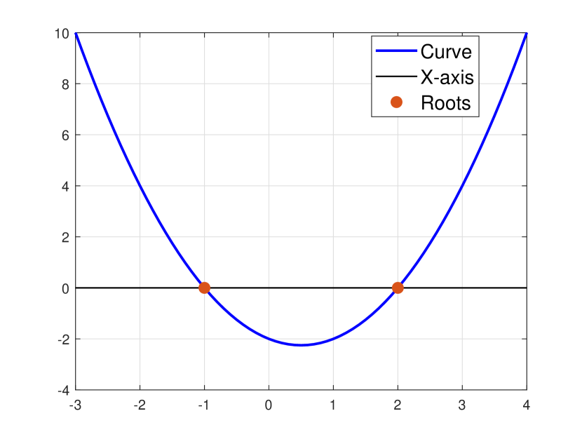
(a)

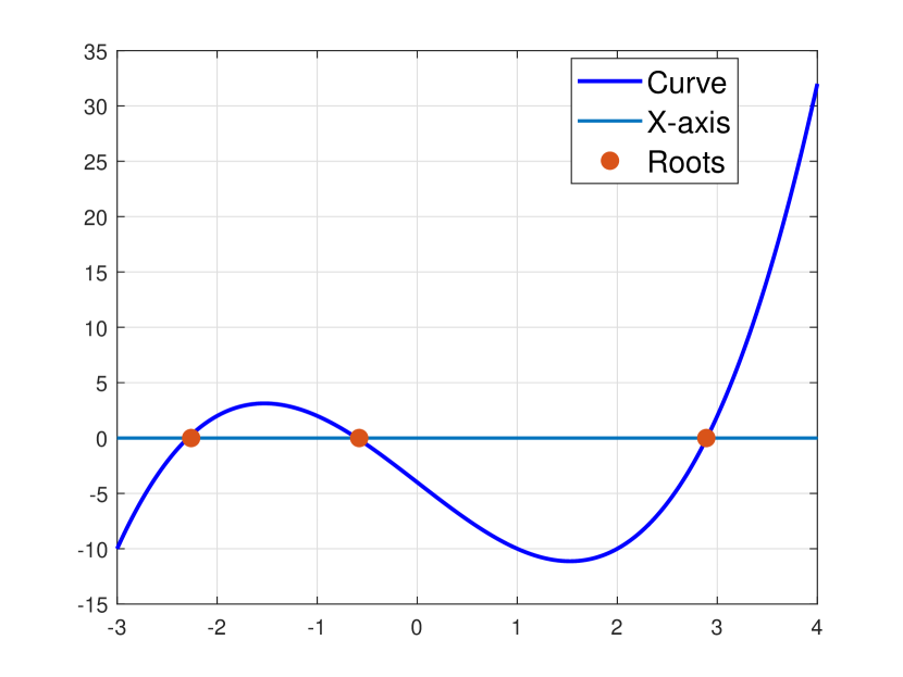
(b)

Figure 2:  The sketch figures for the curve of the function $f(x)=x^{m-1}-\alpha x-\beta$ for odd and even case: a) odd $m$ case: $m=3,\alpha=1,\beta=2$; b) even $m$ case: $m=4,\alpha=7,\beta=4$.

Remark 2.

Note that both $\alpha$ and $\beta$ are the function of $\mathbf{u}$. For simplicity, we omit the variable $\mathbf{u}$ in the notations. We discuss the sign of $\alpha$ and $\beta$ for different orders $m$. When $m$ is odd, since $\alpha(-\mathbf{u})=-\alpha(\mathbf{u})$, we can always select the value where $\alpha>0$. For $\beta$ which is the summation of $n$ non-negative terms, it holds that $\beta\geq 0$. However, considering the constraint in (20) and (21), all $n$ terms $u_{i}$ cannot be equal to 0 simultaneously. Therefore, we can finally conclude that $\beta>0$. A similar analysis can be proceeded for the even $m$ case, and it holds that $\alpha>0$ and $\beta\geq 0$.

Then, as can be observed from (19), each $u_{i}$ can be one of the roots of $(m-1)$-order polynomial $u_{i}^{m-1}-\alpha u_{i}-\beta=0$. Note that in this paper, we only discussed the real solutions, consistent with the previous work [5]. By plotting the function curves with the form of $f(x)=x^{m-1}-\alpha x-\beta$ for odd and even two cases, it can be observed from Fig 2 that when $m$ is odd, there are at most two real roots for $u_{i}^{m-1}-\alpha u_{i}-\beta=0$, while $m$ is even, the number turns to be three ones. Therefore, throughout the following contents, we will separately discuss the odd and even $m$ cases. Note that such an observation and classification rule is consistent with the discussion presented in the previous work [5]. The differences lie in that [5] focuses on the original model (15), while this paper analyzes the reformulated one (16).

And the following Lemma concludes the structure and number of all the stationary solutions for model (16):

Lemma 1.

i): when $m$ is odd, all the stationary points of model (16), $\mathbf{u}=[u_{1},u_{2},\dots,u_{n}]^{\mathrm{T}}\in\mathbb{R}^{n\times 1}$, are with the structure as follows:

$$\mathbf{u}=\mathbf{P}[a\mathbf{1}_{k}^{\mathrm{T}},b\mathbf{1}_{n-k}^{\mathrm{T}}]^{\mathrm{T}},$$ (24)

where $a=\sqrt{\frac{n-k}{kn}}>0$ and $b=-\sqrt{\frac{k}{(n-k)n}}<0$ vary with $k$, where $1\leq k\leq\lceil n/2\rceil$, ($\lceil n/2\rceil$ denotes the integrate that is no larger than $n/2$) and $\mathbf{P}\in\mathbb{R}^{n\times n}$ is a permutation matirx.

ii): when $m$ is even, all the stationary points of model (16), $\mathbf{u}=[u_{1},u_{2},\dots,u_{n}]^{\mathrm{T}}\in\mathbb{R}^{n\times 1}$, are with the structure as follows:

$$\mathbf{u}=\mathbf{P}[a\mathbf{1}_{k}^{\mathrm{T}},b\mathbf{1}_{n-k}^{\mathrm{T}}]^{\mathrm{T}}$$ (25)

or

$$\mathbf{u}=\mathbf{P}[c\mathbf{1}_{p}^{\mathrm{T}},d\mathbf{1}_{q}^{\mathrm{T}},e\mathbf{1}_{s}^{\mathrm{T}}]^{\mathrm{T}}$$ (26)

where $a=\sqrt{\frac{n-k}{kn}}>0$ and $b=-\sqrt{\frac{k}{(n-k)n}}<0$ vary with $k$, where $1\leq k\leq\lceil n/2\rceil$, and $\mathbf{P}\in\mathbb{R}^{n\times n}$ is a permutation matirx; where $1\leq p,q,s\leq n-1$ and $p+q+s=n$. Note that there is no explicit expression for the variables $c,d,e$ in (26).

iii): when $m\geq 3$ is odd and $n\geq 3$, the number of all the stationary points of model (16) is equal to $K_{m,n}=2^{n-1}-1$.

iv): when $m\geq 3$ is even and $n\geq 3$ , the number of all the stationary points of model (16) is equal to

$$K_{m,n}=\begin{cases}\frac{3^{n-1}-1}{2},\quad n\geq 3,m\geq 4\\ 6,\quad\quad\quad n=3,m\geq 6\end{cases}.$$ (27)

Proof.

Equivalently, for (19), there are $n$ equations with the form of

$$u_{i}^{m-1}-\alpha u_{i}-\beta=0\quad(i=1,2,\dots,n).$$ (28)

In term of (i), when $m$ is odd, there are two real roots for (28), denoted by $a,b$ for simplicity. It can be checked that all $n$ variable $u_{i}$ cannot simultaneously be $a$ or $b$. Otherwise, we will derive $u_{1}=u_{2}=\dots=u_{n}$, which is contradicted with the constraints in (16).

Therefore, there are at most $n-1$ variable $u_{i}$ can be the same one. For example, assume that the first $k$ ($1\leq k\leq n-1$) variables are the same, and the last $n-k$ fractions are the other one. The form of the solution is given by

$$u_{1}=u_{2}\cdots=u_{k}=a, u_{k+1}=u_{k+2}\cdots=u_{n}=b.$$ (29)

Considering the two constraints in (16), we have that

$$\begin{cases}ka^{2}+(n-k)b^{2}=1\\ ka+(n-k)b=0\end{cases}.$$ (30)

Then, it can be derived that

$$\begin{cases}a=\sqrt{\frac{n-k}{kn}}\\ b=-\sqrt{\frac{k}{(n-k)n}}\end{cases},\quad or\quad\begin{cases}a=-\sqrt{\frac{n-k}{kn}}\\ b=\sqrt{\frac{k}{(n-k)n}}\end{cases},$$ (31)

where $a,b$ vary with $k$. Furthermore, note that because $f(-\mathbf{u})=-f(\mathbf{u})$ when $m$ is odd, we thus can only reserve the former one solution in (31) where $a>0$ . Then, the structure of all solutions can be denoted by permuting the indices of $i$ by a permutation matrix $\mathbf{P}$, which then can be expressed as the form in (24).

In term of (ii), when $m$ is even, there are at most three real roots for (28). Similarly, all $n$ variables cannot be the same one, indicating that there are at least two different values concerning the components of $\mathbf{u}$. Then, the analysis can be similarly proceeded as that in (i) and the structure of the solution will be given by (25) and (26). Note that for (25), the value of $a$ and $b$ can be the same as the odd $m$ cases. While for (26), since we have three unknown variables $c,d,e$ but only two constraints, we cannot obtain the explicit expression for $c,d,e$.

In term of (iii), since each $u_{i}$ can be selected as one of two real roots, the total combination numbers are given by $2^{n}$. First, the case that all $n$ $u_{i}$ are the same one should be excluded, as analyzed before. In addition, in the left $2^{n}-2$ combinations, it contains repeated same solutions, for example, $[a\mathbf{1}_{k}^{\mathrm{T}},b\mathbf{1}_{n-k}^{\mathrm{T}}]^{\mathrm{T}}$ and $[b\mathbf{1}_{k}^{\mathrm{T}},a\mathbf{1}_{n-k}^{\mathrm{T}}]^{\mathrm{T}}$ can be treated as the same one solution. This is the reason that we constraint $1\leq k\leq\lceil n/2\rceil$, since the solutions where $\lceil n/2\rceil\leq k\leq n-1$ can be considered as the same one. Therefore, the total number of feasible solutions is given by $\frac{2^{n}-2}{2}=2^{n-1}-1$.

In term of (iv), for the even $m$ case, it can be analyzed in a similar way to that in (iii). Since one special case of $n=3,m=4$ is excluded out of the scope, as explained in Remark 1, the number of all solutions is separately discussed from two different cases. In the first case where $n=3,m\geq 6$, it is easy to conclude that there are totally 6 solutions, counting three ones for both (25) and (26). In the second case where $n\geq 3,m\geq 4$, similar to the analysis for the odd $m$ case, the number of all stationary solutions is eventually given by $\frac{3^{n-1}-1}{2}$. And the proof is complete. ∎

Remark 3.

Note that in (25) and (26), we use five notations from $a$ to $e$ to distinguish the two different structures of the solutions for the even $m$ cases. We wish that such a distinction will not cause ambiguity concerning the fact that there are at most three different real roots for $u_{i}^{m-1}-\alpha u_{i}-\beta=0\quad(i=1,2,\dots,n)$ when $m$ is even.

After having investigated the structure of all stationary solutions, the following lemma can be established to reveal the relationship between the vector in the frame (which is the generators of the corresponding regular simplex tensor) and all stationary solutions:

Lemma 2.

The vectors in the regular simplex frame, i.e., $\mathbf{w}_{1},\ldots,\mathbf{w}_{n}$, correspond to eigenpairs when $k=1$ in both (24) and (25).

Proof.

Concerning the vectors in the regular simplex frame $\mathbf{W}=[\mathbf{w}_{1},\ldots,\mathbf{w}_{n}]\in\mathbb{R}^{(n-1)\times n}$, it holds that $\mathbf{w}_{i}^{\mathrm{T}}\mathbf{w}_{i}=1,\mathbf{w}_{i}^{\mathrm{T}}\mathbf{w}_{j}=\alpha=-\frac{1}{n-1}$ for $i\neq j$. It can be calculated that when $\mathbf{v}=\mathbf{w}_{j}$, it holds that

$$\mathbf{u} =\sqrt{\frac{n-1}{n}}{\mathbf{W}}^{\mathrm{T}}{\mathbf{w}_{j}}=[u_{1},u_{2},\dots,u_{n}]^{\mathrm{T}}$$

$$=\sqrt{\frac{n-1}{n}}[\alpha,\dots,\alpha,\underbrace{1}_{j},\alpha,\dots,\alpha]^{\mathrm{T}}\in\mathbb{R}^{n\times 1},$$ (32)

It can be checked that $\mathbf{u}$ with the above form satisfies the two constraints in (16). Clearly, when $\mathbf{v}=\mathbf{w}_{j}$, $\mathbf{u}$ in (4) correspond to the solutions of $k=1$ of (24) and (25), and it holds for both odd and even cases. By the equivalence between (15) and (16), all the vectors in the regular simplex frame, i.e., $\mathbf{w}_{1},\ldots,\mathbf{w}_{n}$, correspond to $n$ eigenpairs of the regular simplex tensor. ∎

5 Structure of all locally optimal points of (16)

We have investigated the structure of all stationary points of (16) in the above section, and also shown that the vectors in the regular simplex frame correspond to the solution of (16) when $k=1$ in (24) and (25). In this section, we are further interested in identifying the local optimality of each eigenpair, i.e., which are the locally maximized, minimized or saddle ones of (16) among these solutions. In other words, we tend to group all these eigenpairs into three classes. For this purpose, it is necessary to introduce the second-order derivative information of the Lagrangian function. For (17), the second-order derivation to $\mathbf{u}$, termed the Hessian matrix, is denoted

$$\triangledown_{\mathbf{u}\mathbf{u}}^{2}L=\mathbf{H}(\mathbf{u})=(m-1)diag(\mathbf{u}^{\circledast^{m-2}})-\alpha\mathbf{I}_{n}.$$ (33)

Similar to the derivation for (7), the locally optimal solutions of (16) can be identified by checking the negative definiteness of the following matrix:

$$\mathbf{M}=(\mathbf{P}_{\mathbf{A}}^{\bot})^{\mathrm{T}}\mathbf{H}(\mathbf{u})\mathbf{P}_{\mathbf{A}}^{\bot}=\mathbf{P}_{\mathbf{A}}^{\bot}\mathbf{H}(\mathbf{u})\mathbf{P}_{\mathbf{A}}^{\bot},$$ (34)

where $\mathbf{A}$ is determined by the two constraints $g_{1}(\mathbf{u})$ and $g_{2}(\mathbf{u})$, which is with the following form:

$$\mathbf{A}=[\triangledown g_{1}(\mathbf{u}),\triangledown g_{2}(\mathbf{u})]=[\mathbf{u},\mathbf{1}_{n}]\in\mathbb{R}^{n\times 2}.$$ (35)

And the detailed explanation for the derivation of (34) are also presented in the Appendix part.

Similarly, we will separately discuss the cases of odd and even order. Meanwhile, as there are three structure as presented from (24) to (26), these three different cases are separately analyzed in the following subsections. The details are as follows.

5.1 Odd $m$ case

In this subsection, we first focus on the tensor with odd $m$, whose solutions are as shown in (24).

Lemma 3.

For the case where $m$ is odd, concerning the solutions with the form of (24): i): when $k=1$ the solutions are the locally maximized points of model (16); ii) when $2\leq k\leq\lceil n/2\rceil$, all the other solutions are the saddle points model (16).

Proof.

Due to the form of $\mathbf{A}$ as shown in (35), $\mathbf{P}_{\mathbf{A}}^{\bot}$ can be further rewritten as

$$\mathbf{P}_{\mathbf{A}}^{\bot} =\mathbf{I}_{n}-\begin{bmatrix}\mathbf{u}&\mathbf{1}_{n}\end{bmatrix}(\begin{bmatrix}\mathbf{u}^{\mathrm{T}}\\ \mathbf{1}_{n}^{\mathrm{T}}\end{bmatrix}\begin{bmatrix}\mathbf{u}&\mathbf{1}_{n}\end{bmatrix})^{-1}\begin{bmatrix}\mathbf{u}^{\mathrm{T}}\\ \mathbf{1}_{n}^{\mathrm{T}}\end{bmatrix}$$

$$=\mathbf{I}_{n}-\begin{bmatrix}\mathbf{u}&\mathbf{1}_{n}\end{bmatrix}(\begin{bmatrix}\mathbf{u}^{\mathrm{T}}\mathbf{u}&\mathbf{u}^{\mathrm{T}}\mathbf{1}_{n}\\ \mathbf{1}_{n}^{\mathrm{T}}\mathbf{u}&\mathbf{1}_{n}^{\mathrm{T}}\mathbf{1}_{n}\\ \end{bmatrix})^{-1}\begin{bmatrix}\mathbf{u}^{\mathrm{T}}\\ \mathbf{1}_{n}^{\mathrm{T}}\end{bmatrix}$$

$$=\mathbf{I}_{n}-(\mathbf{u}\mathbf{u}^{\mathrm{T}}+\frac{1}{n}\mathbf{1}_{n}\mathbf{1}_{n}^{\mathrm{T}}).$$ (36)

where we use the equation $\mathbf{u}^{\mathrm{T}}\mathbf{1}_{n}=\mathbf{1}_{n}^{\mathrm{T}}\mathbf{u}=0$.

In addition, by considering the structure of $\mathbf{u}$ as shown in (24) and (25) in Lemma 1, $\mathbf{u}\mathbf{u}^{\mathrm{T}}$ can be presented in the block form, which follows:

$$\mathbf{u}\mathbf{u}^{\mathrm{T}} =\begin{bmatrix}a^{2}\mathbf{J}_{k}&ab\mathbf{J}_{k\times(n-k)}\\ ab\mathbf{J}_{(n-k)\times k}&b^{2}\mathbf{J}_{(n-k)}\end{bmatrix}$$

$$=\begin{bmatrix}a^{2}\mathbf{J}_{k}&-\frac{1}{n}\mathbf{J}_{k\times(n-k)}\\ -\frac{1}{n}\mathbf{J}_{(n-k)\times k}&b^{2}\mathbf{J}_{(n-k)}\end{bmatrix},$$ (37)

where based on (31), it holds that

$$ab=-\frac{1}{n}.$$ (38)

Similarly, $\frac{1}{n}\mathbf{1}_{n}\mathbf{1}_{n}^{\mathrm{T}}$ can also be expressed as

$$\frac{1}{n}\mathbf{1}_{n}\mathbf{1}_{n}^{\mathrm{T}}=\begin{bmatrix}\frac{1}{n}\mathbf{J}_{k}&\frac{1}{n}\mathbf{J}_{k\times(n-k)}\\ \frac{1}{n}\mathbf{J}_{(n-k)\times k}&\frac{1}{n}\mathbf{J}_{(n-k)}\end{bmatrix}.$$ (39)

Summing (5.1) and (39) yields

$$\mathbf{u}\mathbf{u}^{\mathrm{T}}+\frac{1}{n}\mathbf{1}_{n}\mathbf{1}_{n}^{\mathrm{T}} =\begin{bmatrix}(a^{2}+\frac{1}{n})\mathbf{J}_{k}&\mathbf{O}_{k\times(n-k)}\\ \mathbf{O}_{(n-k)\times k}&(b^{2}+\frac{1}{n})\mathbf{J}_{(n-k)}\end{bmatrix}$$

$$=\begin{bmatrix}\frac{1}{k}\mathbf{J}_{k}&\mathbf{O}_{k\times(n-k)}\\ \mathbf{O}_{(n-k)\times k}&\frac{1}{n-k}\mathbf{J}_{(n-k)}\end{bmatrix},$$ (40)

where for the second equation, we utilize

$$a^{2}+\frac{1}{n}=(\sqrt{\frac{n-k}{kn}})^{2}+\frac{1}{n}=\frac{n-k}{kn}+\frac{1}{n}=\frac{1}{k}.$$

Similarly, we derive that

$$b^{2}+\frac{1}{n}=\frac{1}{n-k}.$$

Substitute (5.1) into (5.1), and we have that

$$\mathbf{P}_{\mathbf{A}}^{\bot} =\begin{bmatrix}\mathbf{I}_{k}-\frac{1}{k}\mathbf{J}_{k}&\mathbf{O}_{k\times(n-k)}\\ \mathbf{O}_{(n-k)\times k}&\mathbf{I}_{(n-k)}-\frac{1}{n-k}\mathbf{J}_{(n-k)}\end{bmatrix}.$$ (41)

In a similar way, by considering the structure of $\mathbf{u}$ as shown in (24) and (25) in Lemma 1, $\mathbf{H}(\mathbf{u})$ can also be presented in the block form, which follows:

$$\mathbf{H}(\mathbf{u})=\begin{bmatrix}\sigma_{a}\mathbf{I}_{k}&\mathbf{O}_{k\times(n-k)}\\ \mathbf{O}_{(n-k)\times k}&\sigma_{b}\mathbf{I}_{(n-k)}\end{bmatrix},$$ (42)

where based on (33), we denote $\sigma_{a}=(m-1)a^{m-2}-\alpha,\sigma_{b}=(m-1)b^{m-2}-\alpha$ for simplicity.

Combining (34), (41) and (42) yields

$$\mathbf{M}=\begin{bmatrix}\sigma_{a}(\mathbf{I}_{k}-\frac{1}{k}\mathbf{J}_{k})&\mathbf{O}_{k\times(n-k)}\\ \mathbf{O}_{(n-k)\times k}&\sigma_{b}(\mathbf{I}_{(n-k)}-\frac{1}{n-k}\mathbf{J}_{(n-k)})\end{bmatrix}.$$ (43)

It can be verified that $\mathbf{I}_{k}-\frac{1}{k}\mathbf{J}_{k}=\mathbf{I}_{k}-\frac{1}{k}\mathbf{1}_{k}\mathbf{1}_{k}^{\mathrm{T}}$ is an idempotent matrix, and its $k$ eigenvalues are 0 and 1 (the number are $k-1$). And similar results for $\mathbf{I}_{(n-k)}-\frac{1}{n-k}\mathbf{J}_{(n-k)}$. Clearly, $\mathbf{M}$ is the direct sum of two matrices, and based on the conclusion in Lemma 6, $n$ eigenvalues of $\mathbf{M}$ are

$$\underbrace{\sigma_{a},\sigma_{a},\dots,\sigma_{a}}_{k-1},\underbrace{\sigma_{b},\sigma_{b},\dots,\sigma_{b}}_{n-k-1},\underbrace{0,0}_{2}.$$ (44)

Due to the fact that each element of $\mathbf{H}_{ii}$ is actually the gradient of $u_{i}^{m-1}-\alpha u_{i}-\beta$, $\sigma_{a}$ and $\sigma_{b}$ actually reflect the descending or ascending trend at the roots. When $m$ is odd, as can be observed from Fig. 2(a), it holds that

$$\mathbf{H}_{ii} =[(m-1)diag(\mathbf{u}^{\circledast^{m-2}})-\alpha\mathbf{I}_{n}]_{ii}$$

$$=\begin{cases}(m-1)a^{m-2}-\alpha=\sigma_{a}>0,\quad\quad u_{i}=a>0\\ (m-1)b^{m-2}-\alpha=\sigma_{b}<0,\quad\quad u_{i}=b<0\\ \end{cases}.$$ (45)

Then, we can conclude that if and only if $k=1$, the $n$ eigenvalues of $\mathbf{M}$ are all non-positive, and thus $\mathbf{M}$ is negative semi-definite, indicating that the corresponding direction $\mathbf{u}$ is the locally maximized one. When $2\leq k\leq\lceil n/2\rceil$, the $n$ eigenvalues of $\mathbf{M}$ contains $k-1$ positive eigenvalues and $n-k-1$ negative ones, indicating that the corresponding direction $\mathbf{u}$ is the saddle one. ∎

5.2 Even $m$ case with (25)

In this subsection, we first focus on the tensor with even $m$, whose solutions are as shown in (25).

Lemma 4.

For the case where $m$ is even, concerning the solutions with the form of (25): i): when $k=1$ the solutions are the locally maximized points of model (16); 2): when $2\leq k\leq\lceil n/2\rceil$, denote

$$l(m,n,k)=(m-1)nk^{m-2}-(n-k)^{m-1}-k^{m-1}$$ (46)

If $l(m,n,k)>0$, the corresponding solutions are the locally minimized points of model (16). If $l(m,n,k)<0$, the solutions are the saddle points of model (16).

Proof.

Note that even though for both odd and even $m$ cases, the eigenvalue distribution of $\mathbf{M}$ is with similar structure as shown above (44), the sign of $\sigma_{a}$ and $\sigma_{b}$ is instead different for odd and even $m$ cases. Different from the conclusion in the odd $m$ case that the sign of $\sigma_{a}$ and $\sigma_{b}$ is definite, in the even $m$ case, we can only determine the sign of $\sigma_{a}>0$, while that of $\sigma_{b}$ may be vary with $k$, which can be observed from Fig 2(b). Due to the fact that $\sigma_{a}>0$, it can be derived that when $k\geq 2$, there are at least one positive eigenvalue $\sigma_{a}>0$, and thus the corresponding eigenpair cannot be locally maximized. Therefore, we only need to analyze the case when $k=1$. First, $\sigma_{b}$ as a function of $k$ can be denoted as

$$\sigma_{b} =(m-1)b^{m-2}-\alpha$$

$$=(m-1)(-\sqrt{\frac{k}{(n-k)n}})^{m-2}-[k(\sqrt{\frac{n-k}{kn}})^{m}+(n-k)(-\sqrt{\frac{k}{(n-k)n}})^{m}]$$

$$=\frac{(m-1)k^{r-1}}{(n-k)^{r-1}n^{r-1}}-\frac{(n-k)^{r}}{k^{r-1}n^{r}}-\frac{k^{r}}{(n-k)^{r-1}n^{r}}$$

$$=\frac{(m-1)nk^{m-2}-(n-k)^{m-1}-k^{m-1}}{(n-k)^{r-1}k^{r-1}n^{r}}$$ (47)

The denominator will always be positive, i.e., $(n-k)^{r-1}k^{r-1}n^{r}>0$. We only focus on the sign of numerator, denoted by

$$l(m,n,k)=(m-1)nk^{m-2}-(n-k)^{m-1}-k^{m-1}$$ (48)

When $k=1$, the numerator equals to $l(m,n,1)=(m-1)n-(n-1)^{m-1}-1$. Since $n\geq 3$ and $m\geq 4$, and both $(m-1)n$ and $(n-1)^{m-1}$ are increase function with respect to $m$ and $n$, it holds that

$$l(m,n,1)=(m-1)n-(n-1)^{m-1}-1\leq 9-2^{3}-1=0$$ (49)

and if and only if when $n=3$ and $m=4$, the equality holds. Since we have excluded the special case of $(m,n)=(4,3)$ out of the discussed scope (see Remark 1 for details), we can conclude that when $k=1$, the eigenvalues are definitely negative, indicating the corresponding eigenpairs are locally maximized. When $2\leq k\leq\lceil n/2\rceil$, there are always $k-1$ positive eigenvalues, so the local optimality will be determined by the sign of $l(m,n,k)$,which will vary for different combinations for $(m,n)$. Therefore, in this proof, we do not intend to exhaust all cases, but conclude as the content as presented in the above lemma. ∎

Therefore, in both odd and even cases, we can conclude that for the solution $\mathbf{u}=\mathbf{P}[a\mathbf{1}_{k}^{\mathrm{T}},b\mathbf{1}_{n-k}^{\mathrm{T}}]^{\mathrm{T}}$ when $k=1$, all the eigenvalue of the corresponding matrix $\mathbf{M}$ are negative, and thus the corresponding eigenpairs are the locally maximized solutions. This is summarized as the following corollary:

Corollary 1.

All vectors in the regular simplex frame are the locally maximized solutions of the corresponding model (15).

5.3 Even $m$ case with (26)

In this part, we analyze the sign of the eigenvalues of $\mathbf{M}$ regarding these eigenpairs with the following structure as shown in (26):

$$\mathbf{u}=[c\mathbf{1}_{p}^{\mathrm{T}},d\mathbf{1}_{q}^{\mathrm{T}},e\mathbf{1}_{s}^{\mathrm{T}}]^{\mathrm{T}}$$ (50)

Without lossing of generality, we assume that the following relationship holds

$$e<d<0<c.$$ (51)

With this assumption, the sign of each diagonal element in the matrix $\mathbf{H}(\mathbf{u})$ can also be determined, which can be observed from Fig. 2(b) and thus follows:

$$\mathbf{H}_{ii} =[(m-1)diag(\mathbf{u}^{\circledast^{m-2}})-\alpha\mathbf{I}_{n}]_{ii}$$

$$=\begin{cases}(m-1)a^{m-2}-\alpha=\sigma_{c}>0,\quad\quad u_{i}=c\\ (m-1)b^{m-2}-\alpha=\sigma_{d}<0,\quad\quad u_{i}=d\\ (m-1)c^{m-2}-\alpha=\sigma_{e}>0,\quad\quad u_{i}=e\\ \end{cases}.$$ (52)

Then, the eigenvalues are sorted in a ascending order as follows:

$$\underbrace{\sigma_{d}=\dots,\sigma_{d}}_{q}<0\leq\underbrace{\sigma_{c}=\dots,\sigma_{c}}_{p}\leq\underbrace{\sigma_{e}=\dots,\sigma_{e}}_{s}.$$ (53)

It should be noted that since we cannot obtain the explicit solution for $\mathbf{u}$ as shown in (50) in this case, it will be difficult to obtain all eigenvalues of $\mathbf{M}$ as can be done for the odd $m$ case and the case 1 in Subsection 5.2. Therefore, in this case, we turn to proving a weaker conclusion: there is at least one positive and negative eigenvalue for $\mathbf{M}$, which can also determine the local optimality of eigenpairs. And the following lemma can be built:

Lemma 5.

For the case where $m$ is even, concerning the solutions with the form of (26), except for the case where $q=1$, the other left solutions are the saddle points of model (16). For $q=1$, it holds that the corresponding solution cannot be a locally maximized one.

Proof.

First, $\mathbf{M}$ is rewritten as:

$$\mathbf{M} =\mathbf{P}_{\mathbf{A}}^{\bot}\mathbf{H}(\mathbf{u})\mathbf{P}_{\mathbf{A}}^{\bot}=(\mathbf{I}_{n}-\mathbf{u}\mathbf{u}^{\mathrm{T}}-\frac{1}{n}\mathbf{1}_{n}\mathbf{1}_{n}^{\mathrm{T}})\mathbf{H}(\mathbf{I}_{n}-\mathbf{u}\mathbf{u}^{\mathrm{T}}-\frac{1}{n}\mathbf{1}_{n}\mathbf{1}_{n}^{\mathrm{T}})$$ (54)

Denote

$$\mathbf{Q}=[\mathbf{q}_{1},\mathbf{q}_{2},\dots,\mathbf{q}_{n}]\in\mathbb{R}^{n\times n}$$ (55)

is an orthogonal matrix, i.e., $\mathbf{Q}^{\mathrm{T}}\mathbf{Q}=\mathbf{Q}\mathbf{Q}^{\mathrm{T}}=\mathbf{I}$. By further considering and utilizing the constraint $\mathbf{u}^{\mathrm{T}}\mathbf{1}_{n}=0$ and $\mathbf{u}^{\mathrm{T}}\mathbf{u}=1$ in the following, we can then set $\mathbf{q}_{1}=\frac{\mathbf{1}_{n}}{\sqrt{n}}$ and $\mathbf{q}_{2}=\mathbf{u}$. Since $\mathbf{Q}$ is an orthogonal one, then $\mathbf{M}$ and $\mathbf{Q}^{\mathrm{T}}\mathbf{M}\mathbf{Q}$ are similar to each other, which will be with the same eigenvalues according to the conclusion in linear algebra.

Then, the following several relationships can be established. It holds that

$$(\mathbf{u}\mathbf{u}^{\mathrm{T}}+\frac{1}{n}\mathbf{1}_{n}\mathbf{1}_{n}^{\mathrm{T}})\mathbf{Q}=[\frac{\mathbf{1}_{n}}{\sqrt{n}},\mathbf{u},\mathbf{0},\dots,\mathbf{0}]$$ (56)

$$\mathbf{H}(\mathbf{u}\mathbf{u}^{\mathrm{T}}+\frac{1}{n}\mathbf{1}_{n}\mathbf{1}_{n}^{\mathrm{T}})\mathbf{Q}=[\frac{\mathbf{H}\mathbf{1}_{n}}{\sqrt{n}},\mathbf{H}\mathbf{u},\mathbf{0},\dots,\mathbf{0}]$$ (57)

$$\mathbf{H}\mathbf{u} =((m-1)diag(\mathbf{u}^{\circledast^{m-2}})-\alpha\mathbf{I}_{n})\mathbf{u}$$

$$=(m-1)\mathbf{u}^{\circledast^{m-1}}-\alpha\mathbf{u}$$

$$=(m-1)\alpha\mathbf{u}+(m-1)\beta\mathbf{1}_{n}-\alpha\mathbf{u}$$

$$=(m-2)\alpha\mathbf{u}+(m-1)\beta\mathbf{1}_{n}$$ (58)

where (19) is utilized in the third rquation. Similarly, we have that

$$\mathbf{H}\mathbf{1}_{n}=(m-1)\mathbf{u}^{\circledast^{m-2}}-\alpha\mathbf{1}_{n}$$ (59)

Furthermore, it can be derived that

$$\mathbf{u}^{\mathrm{T}}\mathbf{H}\mathbf{u}=(m-2)\alpha,\quad\mathbf{1}_{n}^{\mathrm{T}}\mathbf{H}\mathbf{1}_{n}=(m-1)\gamma-n\alpha,\quad\mathbf{u}^{\mathrm{T}}\mathbf{H}\mathbf{1}_{n}=\mathbf{1}_{n}^{\mathrm{T}}\mathbf{H}\mathbf{u}=n(m-1)\beta,$$ (60)

where $\gamma=\mathbf{1}_{n}^{\mathrm{T}}\mathbf{u}^{\circledast^{m-2}}=\sum u_{i}^{m-2}>0$ for even $m$ case, and we use that $\mathbf{u}^{\mathrm{T}}\mathbf{u}^{\circledast^{m-2}}=n\beta$.

Substitute (56) $\sim$ (60) into $\mathbf{Q}^{\mathrm{T}}\mathbf{M}\mathbf{Q}$, and we can obtain that

$$\mathbf{Q}^{\mathrm{T}}\mathbf{M}\mathbf{Q}=\left[\begin{array}[]{cc}\mathbf{O_{2}}&\mathbf{O}_{2\times(n-2)}\\ \mathbf{O}_{(n-2)\times 2}&\mathbf{Z}^{\mathrm{T}}\mathbf{H}\mathbf{Z}\end{array}\right]$$ (63)

where

$$\mathbf{Z}=\mathbf{Q}_{:,3:n}=[\mathbf{q}_{3},\mathbf{q}_{4},\dots,\mathbf{q}_{n}]\in\mathbb{R}^{n\times(n-2)}$$ (64)

is a column-orthogonal matrix that satisfies $\mathbf{Z}^{\mathrm{T}}\mathbf{Z}=\mathbf{I}_{n-2}$.

Assuming that the $n-2$ eigenvalues of $\mathbf{Z}^{\mathrm{T}}\mathbf{H}\mathbf{Z}$ are denoted by $\lambda_{1},\lambda_{1},\dots,\lambda_{n-2}$. Based on the conclusion in Lemma 6, the $n$ eigenvalues of $\mathbf{Q}^{\mathrm{T}}\mathbf{M}\mathbf{Q}$ and $\mathbf{M}$ can be given by $\lambda_{1},\lambda_{1},\dots,\lambda_{n-2},0,0$. Therefore, the following task is to determine the $n-2$ eigenvalues of $\mathbf{Z}^{\mathrm{T}}\mathbf{H}\mathbf{Z}$. However, this is still a tough problem. By utilizing the conclusion in Lemma 9, we further analyze the eigenvalues distribution of

$$\mathbf{H}\mathbf{Z}\mathbf{Z}^{\mathrm{T}}=\mathbf{H}(\mathbf{I}_{n}-\mathbf{u}\mathbf{u}^{\mathrm{T}}-\frac{1}{n}\mathbf{1}_{n}\mathbf{1}_{n}^{\mathrm{T}})=\mathbf{H}-\mathbf{H}(\mathbf{u}\mathbf{u}^{\mathrm{T}}+\frac{1}{n}\mathbf{1}_{n}\mathbf{1}_{n}^{\mathrm{T}}).$$ (65)

Definitely, its $n$ eigenvalues are also given by $\mathbf{\Sigma}=diag(0,0,\lambda_{1},\lambda_{2},\dots,\lambda_{n-2})$.

Since $\mathbf{H}$ has been a diagonal matrix, and its eigenvalues are easy to be determined as presented in (53). So, the following main task is to determine the eigenvalues of $-\mathbf{H}(\mathbf{u}\mathbf{u}^{\mathrm{T}}+\frac{1}{n}\mathbf{1}_{n}\mathbf{1}_{n}^{\mathrm{T}})$. A similar orthogonal transformation by $\mathbf{Q}$ is also first performed on this matrix and eventually, the matrix $-\mathbf{Q}^{\mathrm{T}}\mathbf{H}(\mathbf{u}\mathbf{u}^{\mathrm{T}}+\frac{1}{n}\mathbf{1}_{n}\mathbf{1}_{n}^{\mathrm{T}})\mathbf{Q}$ is with the following structure:

$$-\mathbf{Q}^{\mathrm{T}}\mathbf{H}(\mathbf{u}\mathbf{u}^{\mathrm{T}}+\frac{1}{n}\mathbf{1}_{n}\mathbf{1}_{n}^{\mathrm{T}})\mathbf{Q}=\begin{bmatrix}g_{11}&g_{12}&0&\dots&0\\ g_{21}&g_{22}&0&\dots&0\\ g_{31}&0&0&\dots&0\\ \vdots\\ g_{n1}&0&0&\dots&0\end{bmatrix}:=\mathbf{G}$$ (66)

where $g_{11}=\alpha-\frac{(m-1)\gamma}{n},g_{22}=-(m-2)\alpha<0,g_{12}=g_{21}=-\sqrt{n}(m-1)\beta\leq 0$ for even $m$ cases, $g_{1j}=g_{j1}=-\frac{(m-1)\mathbf{q}_{j}^{\mathrm{T}}\mathbf{u}^{\circledast^{m-2}}}{\sqrt{n}},j=3,4,\dots,n$,

With this form, we then analyze the sign of the eigenvalue of $\mathbf{G}$, denoted in a descend order $\varepsilon_{1}\leq\varepsilon_{2}\leq\dots\leq\varepsilon_{n}$, which can be uniformly transformed into finding the roots of the characteristic polynomial of

$$f(\varepsilon) =det(\mathbf{G}-\varepsilon\mathbf{I})$$

$$=(g_{22}-\varepsilon)(-\varepsilon)^{n-2}det(g_{11}-\varepsilon-\begin{bmatrix}g_{21}\\ g_{31}\\ \vdots\\ g_{n1}\end{bmatrix}^{\mathrm{T}}\begin{bmatrix}g_{22}-\varepsilon&0&\dots&0\\ 0&-\varepsilon&0&\dots&0\\ \vdots\\ g_{n1}&0&0&\dots&-\varepsilon\end{bmatrix}^{-1}\begin{bmatrix}g_{12}\\ 0\\ \vdots\\ 0\end{bmatrix})$$

$$=(g_{22}-\varepsilon)(-\varepsilon)^{n-2}(g_{11}-\varepsilon-\frac{g_{12}^{2}}{g_{22}-\varepsilon})$$

$$=-(-\varepsilon)^{n-2}(\varepsilon^{2}-(g_{11}+g_{22})\varepsilon+(g_{11}g_{22}-g_{12}^{2})$$ (67)

where in the second equation, we block the matrix into $1\times 1$ and $(n-1)\times(n-1)$ and then utilize (80).

When $f(\varepsilon)=0$, it can be observed from (5.3) that it has $(n-2)$-fold roots at $\varepsilon=0$. Therefore, in the following, we further need to determine the sign of the left two non-zero roots, which can be calculated by

$$z(\varepsilon)=\varepsilon^{2}-(g_{11}+g_{22})\varepsilon+(g_{11}g_{22}-g_{12}^{2})$$ (68)

Clearly, $z(\varepsilon)$ is an univariate quadratic equation. On the one hand, the axis of symmetry is given by $g_{11}+g_{22}$. Since

$$\gamma =\sum\limits_{i=1}^{n}u_{i}^{m-2}=(\sum\limits_{i=1}^{n}u_{i}^{m-2})(\sum\limits_{i=1}^{n}u_{i}^{2})=\sum\limits_{i=1}^{n}u_{i}^{m}+\sum\limits_{i,j=1}^{n}u_{i}^{m-2}u_{j}^{2}=\alpha+\theta$$ (69)

where $\theta>0$ for even $m$ cases due to each summation term in $\theta$ is a positive one. It can be checked that

$$tr(\mathbf{G}) =g_{11}+g_{22}=\alpha-(m-1)\gamma/n-(m-2)\alpha$$

$$=-(\frac{m-1}{n}+m-3)\alpha-\frac{m-1}{n}\theta<0,$$ (70)

On the other hand, the discriminant can be computed by $\Delta=(g_{11}+g_{22})^{2}-4(g_{11}g_{22}-g_{12}^{2})=(g_{11}-g_{22})^{2}+4g_{12}^{2}\geq 0$. Therefore, the other two non-zero eigenvalues of $\mathbf{G}$ are given by

$$\varepsilon_{1}=\frac{(g_{11}+g_{22})-\sqrt{\Delta}}{2},\varepsilon_{2}=\frac{(g_{11}+g_{22})+\sqrt{\Delta}}{2}.$$ (71)

In addition, based on the fact that the axis of symmetric is negative by (5.3), we also have that $\varepsilon_{1}<0$, while the sign of $\varepsilon_{2}$ cannot be determined. Furthermore, since

$$z(g_{11})=z(g_{22})=-g_{12}^{2}<0,$$ (72)

it also holds that $\varepsilon_{2}>g_{11}$, and $\varepsilon_{2}>g_{22}$.

So far, we have analyzed the eigen-structure of $\mathbf{G}$, and according to (66), the $n$ eigenvalues of $-\mathbf{H}(\mathbf{u}\mathbf{u}^{\mathrm{T}}+\frac{1}{n}\mathbf{1}_{n}\mathbf{1}_{n}^{\mathrm{T}})$ can be naturally determined, which contains $n-2$ zero roots and 2 non-zero ones $\varepsilon_{1},\varepsilon_{2}$. We sort these roots in a ascending order as follows, which may have two cases:

$$Case\quad 1:\varepsilon_{1}<\varepsilon_{2}<\underbrace{0,0,\dots,0}_{n-2}$$ (73)

or

$$Case\quad 2:\varepsilon_{1}<\underbrace{0,0,\dots,0}_{n-2}<\varepsilon_{2}$$ (74)

Then, by (65), we trun to analyzing the eigenvalues and tend to show that there are at least one positive and negative eihenvalues for $\mathbf{H}\mathbf{Z}\mathbf{Z}^{\mathrm{T}}$, when we have clearly known the eigenvalues distribution of its divided two parts $\mathbf{H}$ (as listed in (53)) and $-\mathbf{H}(\mathbf{u}\mathbf{u}^{\mathrm{T}}+\frac{1}{n}\mathbf{1}_{n}\mathbf{1}_{n}^{\mathrm{T}})$ (as listed in (73) or (74)). Two cases are discussed as follows:

Case 1: Since $p\geq 1,q\geq 1,s\geq 1$ and $p+q+s=n$, the number of positive eigenvalues for matrix $\mathbf{H}$ holds that $p+s\geq 2$. We first focus on the case 1 shown in (73). by using the Weyl theorem in Lemma 8, there is also at least one negative eigenvalue. When $p+s\geq 3$, by using the Weyl theorem in Lemma 8, there is also at least one positive eigenvalue for $\mathbf{H}\mathbf{Z}\mathbf{Z}^{\mathrm{T}}$. The only left one situation that need to be proved is the case of $p+s=2$ (equivalently, $p=1,s=1,q=n-2$). In this case, there are only two positive eigenvalues $\sigma_{c}\leq\sigma_{e}$ for the matrix $\mathbf{H}$, and the two non-zero roots $\varepsilon_{1}\leq\varepsilon_{2}$ for $-\mathbf{H}(\mathbf{u}\mathbf{u}^{\mathrm{T}}+\frac{1}{n}\mathbf{1}_{n}\mathbf{1}_{n}^{\mathrm{T}})$.

The following inequality holds that

$$n\sigma_{d}<tr(\mathbf{H})=(m-1)\gamma-n\alpha={p}\sigma_{c}+{q}\sigma_{d}+{s}\sigma_{e}<n\sigma_{e}$$ (75)

we can conclude

$$\sigma_{c}+\varepsilon_{2} >\frac{tr(\mathbf{H})}{n}+g_{11}\geq 0$$ (76)

For the case $m=4$, we can further have that

$$(u_{i}-c)(u_{i}-d)(u_{i}-e)=u_{i}^{m-1}-\alpha u_{i}-\beta$$ (77)

which will deduce that $c+d+e=0$. Then, solving the following system

$$\begin{cases}pc^{2}+qd^{2}+se^{2}=1\\ pc+qd+se=1\\ c+d+e=0\end{cases}.$$ (78)

will derive that $d=0$, and $c=-e,\sigma_{c}=\sigma_{e}$. Combining with (76), it holds that $\sigma_{e}+\varepsilon_{2}\geq 0$. Using the Weyl theorem in Lemma 8, it can be concluded that there is also at least one positive eigenvalue for $\mathbf{H}\mathbf{Z}\mathbf{Z}^{\mathrm{T}}$.

For the even $m\geq 6$ cases, we cannot directly obtain the new constraint $c+d+e=0$ by (77). However, as can be seen from Fig 2 and Lemma 1, the numer of all eigenpairs is only determined by dimension $n$ in both odd and even $m$ cases, and this indicates that for the even $m\geq 6$ cases, the same conclusion with the $m=4$ case can be arrived, which will also conclude that $\sigma_{e}+\varepsilon_{2}\geq 0$, indicating that there is also at least one positive eigenvalue for $\mathbf{H}\mathbf{Z}\mathbf{Z}^{\mathrm{T}}$. So far, we have shown that there are at least one positive and negative eigenvalue for $\mathbf{H}\mathbf{Z}\mathbf{Z}^{\mathrm{T}}$ in all conbinations for case 1.

Case 2: The analysis of case 2 is very similar to that for case 1. Clearly, for the case 2 shown in (74), since the number of positive eigenvalues for matrix $\mathbf{H}$ holds that $p+s\geq 2$, by using the Weyl theorem in Lemma 8, there is always at least one positive eigenvalue for $\mathbf{H}\mathbf{Z}\mathbf{Z}^{\mathrm{T}}$. When $q>2$, by using the Weyl theorem in Lemma 8, there is also at least one negative eigenvalue for $\mathbf{H}\mathbf{Z}\mathbf{Z}^{\mathrm{T}}$. The only left one situation that need to be proved is the case of $q=1$. For $q=1$, it still holds that there is always at least one positive eigenvalue, indicating that it cannot be a locally maximized one. To determine whether it is a saddle or locally minimized one remains unsolved. The proof for the lemma is complete.

∎

6 Future Work

The regular simplex tensor is a newly-emerging concept and has received some attentions since its proposal. In this part, we will discuss some interesting issues that are worth studying in the future.

1. One widely researched issue concerning the tensor eigenpair concept is to identify whether the eigenpairs obtained by the tensor power method is robust or not. The detailed definition for robust eigenpairs can refer to Theorem 3.2 of Ref [23]. Concerning this subject, it has been discussed in Ref [23] but is not comprehensively addressed, which was claimed as the following conjecture:

Conjecture 1 (Conjecture 4.7 in Ref [23] ).

The robust eigenvectors of a regular simplex tensor are precisely the vectors in the frame.

A rigorous and complete theoretical proof is one of the following tasks to be paid attentions.

2. Consider the following more generalized construction of regular simplex tensor

$$\mathcal{S}:=\sum_{i=1}^{n}\lambda_{k}\mathbf{w}_{i}^{\circ m}$$ (79)

where the weight factors $\lambda_{k}$ is included in each term, which we would like to term as the weighted regular simplex tensor. In this paper, we only consider one special case where all $\lambda_{k}$ are equal to 1, as defined in (9). The above weighted version could be more generalized. What is the eigen-structure of its eigenpairs? Whether the conclusion in conjecture 1 can be extended into the generalized weighted regular simplex tensor? These remain open problems.

3. The other conjectures claimed in the original reference [23] are also worth investigating in the next stage. One can refer to Conjecture 4.8 and 5.2 for details.

7 Appendix

In this appendix part, we will provide some important theorems and lemmas used in our proof. In addition, the detailed explanations for the second-order necessary condition is also presented.

Lemma 6.

(Ref [34]) Suppose that $(\lambda_{i},\mathbf{u}_{i})$ ($i=1,2,\dots,n$), $(\sigma_{j},\mathbf{v}_{j})$ ($j=1,2,\dots,m$) are eigenpairs of $\mathbf{A}$ and $\mathbf{B}$, respectively. The ($n+m$) eigenpairs of $\mathbf{A}\oplus\mathbf{B}$ is $(\lambda_{i},\begin{bmatrix}\mathbf{u}_{i}\\ \mathbf{0}_{m}\end{bmatrix})$, $(\sigma_{j},\begin{bmatrix}\mathbf{0}_{n}\\ \mathbf{v}_{j}\end{bmatrix})$ ($i=1,2,\dots,n$, $j=1,2,\dots,m$).

Lemma 7.

(Ref [34]) Assume that a matrix with a size of $(n+m)\times(n+m)$, can be further divided into $n\times n$ and $m\times m$ two blocks, its determinant can be calculated by

$$det\left[\begin{array}[]{ll}\mathbf{A}&\mathbf{B}\\ \mathbf{C}&\mathbf{D}\end{array}\right]=det(\mathbf{D})det\left(\mathbf{A}-\mathbf{B}\mathbf{D}^{-1}\mathbf{C}\right)$$ (80)

when the matrix $\mathbf{D}$ is assumed to be an inverse one.

Lemma 8 (Weyl Theorem).

Assume that $\mathbf{A}$, $\mathbf{B}\in\mathbb{R}^{n\times n}$ are Hermitian matrix, and the eigenvalues are sorted in a ascending order.

$$\lambda_{1}(\mathbf{A}) \leq\lambda_{2}(\mathbf{A})\leq\cdots\leq\lambda_{n}(\mathbf{A})$$ (81)

$$\lambda_{1}(\mathbf{B}) \leq\lambda_{2}(\mathbf{B})\leq\cdots\leq\lambda_{n}(\mathbf{B})$$

$$\lambda_{1}(\mathbf{A}+\mathbf{B}) \leq\lambda_{2}(\mathbf{A}+\mathbf{B})\leq\cdots\leq\lambda_{n}(\mathbf{A}+\mathbf{B})$$

Then, the following inequalities hold:

$$\lambda_{i}(\mathbf{A}+\mathbf{B})\geqslant\left\{\begin{array}[]{c}\lambda_{i}(\mathbf{A})+\lambda_{1}(\mathbf{B})\\ \lambda_{i-1}(\mathbf{A})+\lambda_{2}(\mathbf{B})\\ \vdots\\ \lambda_{1}(\mathbf{A})+\lambda_{i}(\mathbf{B})\end{array}\right.$$ (82)

and

$$\lambda_{i}(\mathbf{A}+\mathbf{B})\leq\left\{\begin{array}[]{c}\lambda_{i}(\mathbf{A})+\lambda_{n}(\mathbf{B})\\ \lambda_{i+1}(\mathbf{A})+\lambda_{n-1}(\mathbf{B})\\ \vdots\\ \lambda_{n}(\mathbf{A})+\lambda_{i}(\mathbf{B})\end{array}\right.$$ (83)

for $i=1,2,\dots,n$.

Lemma 9.

(Ref [34]) Given the $m\times n$ matrix $\mathbf{A}$ and the $n\times m$ matrix $\mathbf{B}$ ( $m<n$), assuming that the $m$ eigenvalues of $\mathbf{A}\mathbf{B}$ are denoted by $\lambda_{1},\lambda_{2},\dots,\lambda_{m}$, then the $n$ eigenvalues of $\mathbf{B}\mathbf{A}$ are given by $\lambda_{1},\lambda_{2},\dots,\lambda_{m},0,0$.

The following theorem is well established for the constrained optimization problem to identify the locally optimal solutions (Page 332 in [24]):

Theorem 1 (Second-order necessary condition).

[24] Suppose that for any vector $\mathbf{w}\in\mathbb{V}$, if

$$\mathbf{w}^{\mathrm{T}}\mathbf{H}(\mathbf{v})\mathbf{w}\leq 0$$ (84)

holds, then $\mathbf{v}$ is a local maximum solution of (3). And for (3), the set $\mathbb{V}$ is defined as

$$\mathbb{V}=\{\mathbf{w}\in\mathbb{R}^{n}|(\triangledown g)^{\mathrm{T}}\mathbf{w}=0\}=\rm Null[(\triangledown g)^{\mathrm{T}}]=\rm Null[\mathbf{A}],$$ (85)

where $\rm Null(\mathbf{A})$ denotes the null space of $\mathbf{A}$ and $\triangledown g=\mathbf{v}$ denotes the gradient of the constraint: $g(\mathbf{v})=\mathbf{v}^{\mathrm{T}}\mathbf{v}-1=0$.

If a stronger condition, i.e., $\mathbf{w}^{\mathrm{T}}\mathbf{H}(\mathbf{v})\mathbf{w}<0$, is satisfied, then, $\mathbf{v}$ is a strict local maximum solution of (3).

In practice, instead of directly utilizing Theorem 1, it is more preferred to identify the local extremum by checking the positive or negative definiteness of the projected Hessian matrix (denoted $\mathbf{P}$). It is calculated by

$$\mathbf{P}=\mathbf{Q}_{2}^{\mathrm{T}}\mathbf{H}(\mathbf{v})\mathbf{Q}_{2},$$ (86)

where $\mathbf{Q}_{2}$ is obtained by QR factorization of $\triangledown g$:

$$\begin{split}\triangledown g&=\mathbf{Q}\begin{bmatrix}\mathbf{R}\\ \mathbf{0}\end{bmatrix}=\begin{bmatrix}\mathbf{Q}_{1}&\mathbf{Q}_{2}\end{bmatrix}\begin{bmatrix}\mathbf{R}\\ \mathbf{0}\end{bmatrix}=\mathbf{Q}_{1}\mathbf{R}\end{split},$$ (87)

where $\mathbf{Q}$ is an orthogonal matrix, and $\mathbf{R}$ is a square upper triangular matrix. In this case, $\mathbf{R}$ is reduced to a scalar since $\triangledown g$ is a column vector and $\mathbf{0}$ is an vector with all elements equal to 0. See more details for this part in Page 337 of [24].

Furthermore, based on (85), we can conclude that $\mathbf{w}$ must also lie in the orthogonal complement space of $\mathbf{v}$. Therefore, $\mathbf{w}$ can be linearly expressed by the column vectors of $\mathbf{P}_{\mathbf{v}}^{\bot}$. Assume that $\mathbf{z}\in\mathbb{R}^{(n-1)\times 1}$ is the coefficient vectors, it holds that $\mathbf{w}=\mathbf{P}_{\mathbf{v}}^{\bot}\mathbf{z}$. Then it can be verified that $\mathbf{v}^{\mathrm{T}}\mathbf{w}=\mathbf{v}^{\mathrm{T}}\mathbf{P}_{\mathbf{v}}^{\bot}\mathbf{z}=\mathbf{v}^{\mathrm{T}}(\mathbf{I}_{n}-\mathbf{v}(\mathbf{v}^{\mathrm{T}}\mathbf{v})^{-1}\mathbf{v}^{\mathrm{T}})\mathbf{z}=\mathbf{0}$ holds. Therefore, (84) can be rewritten as $\mathbf{w}^{\mathrm{T}}\mathbf{H}(\mathbf{v})\mathbf{w}=\mathbf{z}^{\mathrm{T}}(\mathbf{P}_{\mathbf{v}}^{\bot})^{\mathrm{T}}\mathbf{H}(\mathbf{v})\mathbf{P}_{\mathbf{v}}^{\bot}\mathbf{z}\leq 0$. Since $\mathbf{z}$ can be arbitrary vectors, checking (84) is equivalent to checking negative semi-definiteness of the matrix, denoted $\mathbf{M}$, with the form of

$$\mathbf{M}=(\mathbf{P}_{\mathbf{v}}^{\bot})^{\mathrm{T}}\mathbf{H}(\mathbf{v})\mathbf{P}_{\mathbf{v}}^{\bot}=(\mathbf{P}_{\mathbf{v}}^{\bot})\mathbf{H}(\mathbf{v})\mathbf{P}_{\mathbf{v}}^{\bot},$$

which corresponds to (7).

Note that there are only one constraint for model (3). When more constraints are included, it can be similarly analyzed. For example. for model (16) with two constraints, $\mathbf{A}$ should be defined as

$$\mathbf{A}=[\triangledown g_{1}(\mathbf{u}),\triangledown g_{2}(\mathbf{u})]=[\mathbf{u},\mathbf{1}_{n}]\in\mathbb{R}^{n\times 2}.$$

And the locally optimal solutions of (16) can be identified by checking the negative definiteness of the matrix as defined in (34).

References

• [1] A. Anandkumar, R. Ge, D. Hsu, S. M. Kakade, and M. Telgarsky, Tensor decompositions for learning latent variable models, The Journal of Machine Learning Research, 15 (2014), pp. 2773–2832.
• [2] J. Chang, Y. Chen, and L. Qi, Computing eigenvalues of large scale sparse tensors arising from a hypergraph, Siam Journal on Scientific Computing, 38 (2016), pp. A3618–A3643.
• [3] L. Chen, L. Han, and L. Zhou, Computing tensor eigenvalues via homotopy methods, SIAM Journal on Matrix Analysis and Applications, 37 (2016), pp. 290–319, https://doi.org/10.1137/15M1010725.
• [4] C. F. Cui, Y. H. Dai, and J. Nie, All real eigenvalues of symmetric tensors, Siam Journal on Matrix Analysis and Applications, 35 (2014).
• [5] A. Czaplinski, T. Raasch, and J. Steinberg, Real eigenstructure of regular simplex tensors, CoRR, abs/2203.01865 (2022), https://doi.org/10.48550/arXiv.2203.01865, https://doi.org/10.48550/arXiv.2203.01865, https://arxiv.org/abs/2203.01865.
• [6] X. Geng, L. Ji, and K. Sun, Principal skewness analysis: algorithm and its application for multispectral/hyperspectral images indexing, IEEE Geoscience and Remote Sensing Letters, 11 (2014), pp. 1821–1825.
• [7] X. Geng and L. Wang, Npsa: Nonorthogonal principal skewness analysis, IEEE Transactions on Image Processing, 29 (2020), pp. 6396–6408.
• [8] C. J. Hillar and L.-H. Lim, Most tensor problems are np-hard, Journal of the ACM (JACM), 60 (2013), p. 45.
• [9] A. Jaffe, R. Weiss, and B. Nadler, Newton correction methods for computing real eigenpairs of symmetric tensors, SIAM Journal on Matrix Analysis and Applications, 39 (2018), pp. 1071–1094, https://doi.org/10.1137/17M1133312, https://doi.org/10.1137/17M1133312.
• [10] B. Jiang, T. Lin, and S. Zhang, A unified adaptive tensor approximation scheme to accelerate composite convex optimization, SIAM Journal on Optimization, 30 (2020), pp. 2897–2926, https://doi.org/10.1137/19M1286025, https://doi.org/10.1137/19M1286025, https://arxiv.org/abs/https://doi.org/10.1137/19M1286025.
• [11] T. G. Kolda, Orthogonal tensor decompositions, SIAM Journal on Matrix Analysis and Applications, 23 (2001), pp. 243–255.
• [12] T. G. Kolda and B. W. Bader, Tensor decompositions and applications, SIAM review, 51 (2009), pp. 455–500.
• [13] T. G. Kolda and J. R. Mayo, Shifted power method for computing tensor eigenpairs, Siam Journal on Matrix Analysis and Applications, 32 (2011), pp. 1095–1124.
• [14] T. G. Kolda and J. R. Mayo, An adaptive shifted power method for computing generalized tensor eigenpairs, Siam Journal on Matrix Analysis and Applications, 35 (2014), pp. 1095–1124.
• [15] P. Koniusz, L. Wang, and A. Cherian, Tensor representations for action recognition, IEEE Transactions on Pattern Analysis and Machine Intelligence, 44 (2022), pp. 648–665, https://doi.org/10.1109/TPAMI.2021.3107160.
• [16] L. D. Lathauwer, B. D. Moor, and J. Vandewalle, A Multilinear Singular Value Decomposition, 2000.
• [17] G. Li, L. Qi, and G. Yu, The z-eigenvalues of a symmetric tensor and its application to spectral hypergraph theory, Numerical Linear Algebra with Applications, 20 (2013), pp. 1001–1029.
• [18] J. Li, K. Usevich, and P. Comon, Globally convergent jacobi-type algorithms for simultaneous orthogonal symmetric tensor diagonalization, SIAM J. Matrix Anal. Appl., 39 (2018), pp. 1–22, https://doi.org/10.1137/17M1116295, https://doi.org/10.1137/17M1116295.
• [19] L.-H. Lim, Singular values and eigenvalues of tensors: a variational approach, in Computational Advances in Multi-Sensor Adaptive Processing, 2005 1st IEEE International Workshop on, IEEE, 2005, pp. 129–132.
• [20] Q. I. Liqun, S. Wenyu, and W. Yiju, Numerical multilinear algebra and its applications, Frontiers of Mathematics in China, 2 (2007), pp. 501–526.
• [21] C. Lu, J. Feng, Y. Chen, W. Liu, Z. Lin, and S. Yan, Tensor robust principal component analysis with a new tensor nuclear norm, IEEE Transactions on Pattern Analysis and Machine Intelligence, 42 (2020), pp. 925–938.
• [22] C. Mu, D. J. Hsu, and D. Goldfarb, Successive rank-one approximations for nearly orthogonally decomposable symmetric tensors, SIAM J. Matrix Anal. Appl., 36 (2015), pp. 1638–1659, https://doi.org/10.1137/15M1010890, https://doi.org/10.1137/15M1010890.
• [23] T. Muller, E. Robeva, and K. Usevich, Robust eigenvectors of symmetric tensors, CoRR, abs/2111.06880 (2021), https://arxiv.org/abs/2111.06880, https://arxiv.org/abs/2111.06880.
• [24] J. Nocedal and S. J. Wright, Numerical Optimization, 1999.
• [25] L. Qi, Eigenvalues of a real supersymmetric tensor, Journal of Symbolic Computation, 40 (2005), pp. 1302–1324.
• [26] L. Qi, D-eigenvalues of diffusion kurtosis tensor, Journal of Computational and Applied Mathematics, 221 (2008), pp. 150–157.
• [27] L. Qi and K. L. Teo, Multivariate polynomial minimization and its application in signal processing, Journal of Global Optimization, 26 (2003), pp. 419–433.
• [28] L. Qi, F. Wang, and Y. Wang, Z-eigenvalue methods for a global polynomial optimization problem, Mathematical Programming, 118 (2009), pp. 301–316.
• [29] L. Qi, X. Zhang, and Y. Chen, A tensor rank theory, full rank tensors and the sub-full-rank property, CoRR, abs/2004.11240 (2020), https://arxiv.org/abs/2004.11240, https://arxiv.org/abs/2004.11240.
• [30] E. Robeva, Orthogonal decomposition of symmetric tensors, SIAM J. Matrix Anal. Appl., 37 (2016), pp. 86–102, https://doi.org/10.1137/140989340, https://doi.org/10.1137/140989340.
• [31] K. Usevich, J. Li, and P. Comon, Approximate matrix and tensor diagonalization by unitary transformations: Convergence of jacobi-type algorithms, SIAM Journal on Optimization, 30 (2020), pp. 2998–3028, https://doi.org/10.1137/19M125950X, https://doi.org/10.1137/19M125950X, https://arxiv.org/abs/https://doi.org/10.1137/19M125950X.
• [32] L. Wang and X. Geng, The real eigenpairs of symmetric tensors and its application to independent component analysis, IEEE Transactions on Cybernetics, (2021), pp. 1–14, https://doi.org/10.1109/TCYB.2021.3055238.
• [33] Y. Wang and L. Qi, On the successive supersymmetric rank-1 decomposition of higher-order supersymmetric tensors, Numerical Linear Algebra with Applications, 14 (2010), pp. 503–519.
• [34] X. Zhang, Matrix analysis and applications, Cambridge University Press, 2017.
• [35] X. Zhao, M. Bai, D. Sun, and L. Zheng, Robust tensor completion: Equivalent surrogates, error bounds, and algorithms, SIAM J. Imaging Sci., 15 (2022), pp. 625–669, https://doi.org/10.1137/21m1429539, https://doi.org/10.1137/21m1429539.