SUNY: A Visual Interpretation Framework for
Convolutional Neural Networks from a Necessary and Sufficient Perspective

Abstract

Researchers have proposed various methods for visually interpreting the Convolutional Neural Network (CNN) via saliency maps, which include Class-Activation-Map (CAM) based approaches as a leading family. However, in terms of the internal design logic, existing CAM-based approaches often overlook the causal perspective that answers the core “why” question to help humans understand the explanation. Additionally, current CNN explanations lack the consideration of both necessity and sufficiency, two complementary sides of a desirable explanation. This paper presents a causality-driven framework, SUNY, designed to rationalize the explanations toward better human understanding. Using the CNN model’s input features or internal filters as hypothetical causes, SUNY generates explanations by bi-directional quantifications on both the necessary and sufficient perspectives. Extensive evaluations justify that SUNY not only produces more informative and convincing explanations from the angles of necessity and sufficiency, but also achieves performances competitive to other approaches across different CNN architectures over large-scale datasets, including ILSVRC2012 and CUB-200-2011.

1 Introduction

In computer vision, an important research direction is to give Convolutional Neural Network (CNN) more transparency to extend its deployment on a broader basis. This paper addresses the eXplainable Artificial Intelligence (XAI) [15] problem corresponding to CNN for natural image classification, i.e., reasoning why a classifier makes particular decisions. Specifically, we study a leading family of techniques called Class-Activation-Maps (CAMs), which present heatmaps highlighting image portions associated with a model’s class prediction.

Figure 1: An example of SUNY explanations. SUNY highlights sufficient and necessary input regions w.r.t. the model’s prediction towards the target class. The 2D saliency map is the first-of-its-kind visual explanation design to the best of our knowledge.

The pioneering method in the family is CAM [47], which produces saliency maps by linearly combining the convolutional feature maps with weights generated by a global average pooling layer. CAM’s structural restriction on the global average pooling layer prohibits its use for general CNNs, and a series of gradient-weighted CAMs [31, 4, 25] have been proposed to overcome the restriction. However, such CAMs suffer from gradients’ saturation and vanishing issues, which cause the resulting explanations to be noisy [12]. To bypass the shortcomings of gradients, Score-CAM [37] and Group-CAM [46] weight the feature maps by contribution scores, referring to the corresponding input features’ importance to the model output.

The design of Score-CAM and Group-CAM to measure the model’s class prediction (outcome) when only keeping specific input features (cause) matches the idea of causal sufficiency (S), while the other aspect, necessity (N), is missing. N refers to changing the hypothetical causes and measuring the outcome differences, and S investigates the outcome stability when specific causes are unchanged. Both are desirable and essential perspectives for a successful explanation [21, 42, 14, 39]. Other CAMs, on the other hand, lack both causal semantics in their design, which makes it challenging to answer the core “why” questions and match human instincts.

Producing a saliency map through causal explanations requires calculating the importance of each cause (e.g., a region of input image or a model filter) when interacting with other causes. Techniques for quantifying the importance of causes consist of two main genres, causal effect [13] and responsibility [6]. Causal effect measures the outcome differences when intervening on the causes; responsibility measures the minimal set of causes needed to change the outcome. In causal effect analysis, the effect of a group of causes is a single value, which cannot be easily attributed to distinguish the importance of each individual cause. Responsibility also fails to provide a decent importance score for a single cause because it measures the number of causes rather than the actual outcome differences. That is, these two causal quantification genres cannot be directly taken to produce a sound saliency map. Furthermore, both causal effect and responsibility typically focus on $N$ and overlook $S$. There are a few works addressing CNN causal explanations by adopting either of these two methods, such as CexCNN [9] and [17]. However, the aforementioned limitations have not yet been carefully addressed. To summarize, current CNN explanations, to some extent, fail in (1) human interpretability (not designed from a causal perspective, like GradCAM), (2) precision (failing to generate decent importance for individual cause, given their basis of causal effect or responsibility), or (3) completeness (missing either N or S perspective, like CexCNN). Therefore, it calls for more research efforts in this demanding field of CNN explanations to fulfill the deficiencies.

Considering the issues mentioned above, we propose an explanation framework called SUfficiency and NecessitY causal explanation (SUNY), which interprets the CNN classifier by analyzing how the cooperation of a single cause and other causes affect the model’s decision. SUNY regards either model filters or input features as the hypothesized causes and quantifies each cause’s importance towards the class prediction from angles of both N and S. Specifically, we draw on the strength of both causal effect and responsibility to propose N-S responsibility, which solves the three issues above by (1) being designed from causality theory that is in line with instinctive human habits; (2) providing importance for each individual cause when interacting with other causes by quantizing the effect on top of responsibility; (3) conducting a bi-directional quantification from both N and S perspectives. Based on the qualitative evaluation, including the semantic evaluation and the sanity check, we demonstrate that SUNY provides a more faithful and interpretable visual explanation for CNN models. Comprehensive experiment evaluations on benchmark datasets, including ILSVRC2012 [30] and CUB-200-2011 [40], validate that SUNY outperforms other popular saliency map-based visual explanation methods. Our key contributions are summarized as follows:

• We propose a novel definition, N-S responsibility, for a bi-directional causal importance quantification for CNNs from N and S perspectives.

• We introduce a flexible framework, SUNY, which can provide valid CNN visual explanations by analyzing either model filters or input features.

• We provide 2D saliency maps for a more informative visual explanation, which is the first 2D visual explanation design of CNN to the best of our knowledge.

• Extensive quantitative and qualitative experiments highlight our explanations’ effectiveness and uncover the potential of SUNY in real-world problem-solving.

2 Related Work

Saliency Map Explanations for CNNs. The class-discri-minative visual explanation is a key tool for CNN interpretation by highlighting important regions corresponding to a model’s particular prediction. Two widely-adopted types are perturbation-based methods [45, 29, 28] and CAMs [47, 31, 4, 33, 37, 46]. Perturbation-based methods such as RISE [28] are inspired by a human-understandable concept of measuring the output when the inputs are perturbed, which is in line with the N causal semantics. Somehow enumerating and examining all possible input perturbations is computationally challenging [18], making such methods infeasible for applications demanding fast explanations.

CAMs compute a weighted sum of feature maps to generate explanations, which are often more computationally efficient. CAM [47] is the pioneering method in this type, which requires a global average pooling layer in the CNN architecture. GradCAM [31] and a series of its variations, such as Grad-CAM++ [4] and SmoothGrad [33], address this structural restriction by using gradients as weights, hence applicable to a broader variety of CNN families. However, gradients knowingly suffer from vanishing issues and introduce noise to the saliency map [12]. To fix the gradient issues, Score-CAM [37] and Group-CAM [46] weight feature maps by their corresponding input features’ contribution to the output, which matches the S perspective of causal semantics and is implicitly consistent with the ideas of perturbation-based methods.

Causal Importance Evaluations. Based on the HP causality [27, 16] introduced by Halpern and Pearl, recent research for causal importance quantification involves two main genres, causal effect and responsibility. The average causal effect [13] measures the expected outcome difference when the values of selected causes are changed, which regards the set of causes as a whole. An individual cause can thus affect the outcome very differently, i.e., receive completely different effect quantification, when being analyzed with different sets of interacting causes [44]. The second genre, the degree of responsibility [6], quantifies the minimal set of causes whose removal leads to a satisfactory outcome change, which overlooks the actual value of the outcome [20, 3]. Besides, current causal effect and responsibility both focus on the N perspective, i.e., the change of causes, and the other S perspective needs to be fulfilled for a thorough explanation [21, 42, 14, 39]. More recent works such as [39] and [19] address this deficiency by measuring the causal importance from both N and S. However, their proposed quantification focuses on the probability of the outcome change when causes are changed (N) or unchanged (S), which also misses the actual outcome value.

Causal Explanations for CNNs. Given recent works on CNN causal explanations, two main groups exist according to the type of the hypothesized causes – the model’s input features or inner filters. As for the first group, [5] and [17] estimate the average causal effect of input features. The Shapley value-inspired methods [34, 8, 22, 35, 1] also implicitly analyze the causality of input features from the S perspective. However, these methods are too computationally intensive or only provide a hazy outline of salient regions. Two CAM-based methods, Score-CAM [37] and Group-CAM [46], as discussed before, can be regarded as partially causal-grounded by analyzing the sufficiency of input features. On the other side, the perturbation-based methods  [45, 29, 28] analyze input features’ necessity.

The second group of methods interprets CNN through the model filter intervention. For example, [24] explores CNN’s inner workings by ranking filters from a layer according to their counterfactual (CF) influence. However, without any visualizations, this causal explanation of CNN is less intuitive than saliency maps. CexCNN [9] provides visualizations with the help of CAMs and uses responsibility to quantify the CNN’s filter importance, which means only the N aspect has been analyzed.

3 CNN Classification as a Causal Mechanism

With a CNN natural image classifier $M$, an input image $I$, and a target class $c$, our goal is to provide saliency maps to highlight which image portions lead to the model’s prediction of $c$ from a causal perspective. First, we recall the definition of causal mechanism as follows.

Causal mechanism [11]. A portable concept explaining how and why the hypothesized causes, in a given context $u$, contribute to a particular outcome.

Next, we define the outcome and causes in our problem, then demonstrate how we establish the causal mechanism and formulate our problem based on it.

Outcome: As a class-discriminative explanation, we directly measure the model’s prediction probability w.r.t. the target class and set it as the outcome.

Causes: Given that existing CNN causal explanations regard input features or model filters as causes, we allow the flexibility of setting either of them as causes. Specifically, a single cause is (1) a region of the image identified by a feature map; or (2) a model filter in a convolutional layer.

When considering input features as causes, the context $u$ is an unknown process determining the combination of image features. Regarding model filters as causes, the context $u$ is the image region on which we apply the model filters. After establishing the causal mechanism, we can quantify the effect of causes by counterfactually intervening on the hypothesized causes and measuring the outcome, whose results can be used as weights for feature maps’ linear combination. Finally, we can produce saliency maps as a causal explanation for the CNN classifier.

4 The Proposed Approach

Figure 2: Overview of SUNY framework. Phase(a) is a forward pass of input image $I$ through a CNN model, where the prediction probability of the target class is $p_{c}(F)$. Phase(b)-(e) present the generation of SUNY-feature (green) and SUNY-filter (blue), respectively, referring to different types of hypothesized causes. Note that they are not simultaneous processes. In Phase(b), we obtain filters and feature maps of a specified layer, and intervene on model filters or the corresponding input features. We get new prediction probabilities after the intervention and calculate N-S Effect, $E_{N}$, $E_{S}$ in Phase(c), which are fed back to Phase(b) to construct hypothesized cause sets $F_{hypN}$ and $F_{hypS}$. Through intervening on $F_{hypN}$ and $F_{hypS}$ (Phase(b)), we can obtain $E_{N}$, $E_{S}$ (Phase(c)) and N-S Responsibilities $R_{N}$ and $R_{S}$ (Phase(d)), which are weights for the linear combination of feature maps. The saliency maps are generated in Phase(e), where we show SUNY-feature results as an example. Implementation details are included in Sec. 4.

4.1 Causal Importance Evaluation

To address the deficiencies of current causal importance evaluations as discussed in Sec. 2, our evaluation should follow the below design requirements:

1. Our method should measure the importance of each individual cause in a group of coordinating causes.

2. Our method should quantify the actual effect towards the outcome and pay attention to both N and S.

The first step of achieving R2 is to define N-S Effect to quantify effects caused by the intervention of removing/keeping specific causes. We denote a set of causes to be analyzed as $F_{*}$, where $F_{*}\subseteq F$ and $F$ is the universal set of all causes. For N Effect, we measure the degree of the outcome change when removing $F_{*}$, as shown in Eqn. (1):

$$E_{N}(F_{*})=\frac{p_{c}(I)-p_{c}({\rm do}\;(F\setminus F_{*}))}{p_{c}(I)},$$ (1)

where ${\rm do}(F\setminus F_{*})$ represents the CF intervention of removing $F_{*}$. And $p_{c}(\mathchoice{\mathbin{\vbox{\hbox{\scalebox{0.5}{$\displaystyle\bullet$}}}}}{\mathbin{\vbox{\hbox{\scalebox{0.5}{$\textstyle\bullet$}}}}}{\mathbin{\vbox{\hbox{\scalebox{0.5}{$\scriptstyle\bullet$}}}}}{\mathbin{\vbox{\hbox{\scalebox{0.5}{$\scriptscriptstyle\bullet$}}}}})$ refers to the model’s prediction probability w.r.t. a target class $c$, where $p_{c}(I)$ is its original value without any intervention; $p_{c}({\rm do}(F\setminus F_{*}))$ represents the value after the removal intervention. A higher $E_{N}(F_{*})$ indicates a more necessary $F_{*}$.

Similarly, S Effect is defined in Eqn. (2):

$$E_{S}(F_{*})=\frac{p_{c}({\rm do}\;(F_{*}))}{p_{c}(I)},$$ (2)

where ${\rm do}(F_{*})$ represents the CF intervention of only keeping $F_{*}$, i.e., removing $\{F\setminus F_{*}\}$. A higher $E_{S}(F_{*})$ indicates a more sufficient $F_{*}$.

To fulfill R1, we provide a quantification to approximate a fair distribution of N-S Effect to a number of causes working cooperatively. Starting from the N aspect, $\forall f_{i}\in F$, where $f_{i}$ is a single cause, we set $F_{*}=\{f_{i}\}$ to calculate $E_{N}(f_{i})$ and construct a set $F_{N}\subseteq F$ by combining the relatively more necessary $f_{i}$. To analyze a single cause $f_{n}\in F_{N}$ when it interacts with different causes, we intervene on $f_{n}$ by removing it together with $F_{N}^{k}$, a set of causes with a varying size $k$. That is, $F_{*}=F_{hypN}(f_{n})=\{f_{n}\cup F_{N}^{k}\}\subseteq F_{N}$ and we can calculate $E_{N}(F_{hypN}(f_{n}))$ based on Eqn. (1). We then equally distribute it to the containing individual causes. Finally, we accumulate all such $F_{hypN}(f_{n})$ by linearly combining the distributed N Effect corresponding to each $f_{n}$ and the result is defined as N Responsibility of $f_{n}$, as defined in Eqn. (3):

$$R_{N}(f_{n})=\sum_{F_{N}^{k}\subseteq\{F_{N}\setminus f_{n}\}}^{k\in[a,b]}\frac{E_{N}(F_{hypN}(f_{n}))}{k+1},$$ (3)

where $a$ and $b$ are the pre-defined minimum and maximum set sizes of $F_{N}^{k}$. In the implementation, we can reduce the amount of computation by setting the values of $a$ and $b$. Also, the sum in Eqn. 3 can be empirically estimated using Monte Carlo sampling.

Similarly, $\forall f_{i}\in F$, we construct $F_{S}$ for analyzing $S$, and $\forall f_{s}\in F_{S}$, we have $F_{*}=F_{hypS}(f_{s})=\{f_{s}\cup F_{S}^{k}\}\subseteq F_{S}$, where $F_{S}^{k}$ is of a varying size. The definition of S Responsibility is provided in Eqn. (4):

$$R_{S}(f_{s})=\sum_{F_{S}^{k}\subseteq\{F_{S}\setminus f_{s}\}}^{k\in[a,b]}\frac{E_{S}(F_{hypS}(f_{s}))}{k+1}.$$ (4)

Additionally, for $f_{n}^{\prime}\in\{F\setminus F_{N}\}$ and $f_{s}^{\prime}\in\{F\setminus F_{S}\}$, we set $R_{N}(f_{n}^{\prime})=0$ and $R_{S}(f_{s}^{\prime})=0$.

Figure 3: Visual comparison of saliency maps from different methods. The first row: a VGG16 trained on CUB-200-2011, and the image is correctly predicted as Gull. The second row: a VGG16 trained on ILSVRC2012, and the image is correctly predicted as Dog-sled.

4.2 SUNY Implementation

We present the implementation of SUNY in Alg. 1 and an visual overview in Fig. 2. Following the definitions in Sec. 4.1, SUNY provides CAM-based causal explanations regarding input features and model filters as hypothesized causes, respectively, represented by the cause type $E$ in Alg. 1 with values “feature” or “filter”. The corresponding explanations are SUNY-feature and SUNY-filter.

Algorithm 1 SUNY: Causal Explanation of CNN

Input Image $I$, model $M$, layer $l$, class $c$, cause type $E$
Output N-S saliency maps: $N_{map}$, $S_{map}$

1:$p_{c}(\mathchoice{\mathbin{\vbox{\hbox{\scalebox{0.5}{$\displaystyle\bullet$}}}}}{\mathbin{\vbox{\hbox{\scalebox{0.5}{$\textstyle\bullet$}}}}}{\mathbin{\vbox{\hbox{\scalebox{0.5}{$\scriptstyle\bullet$}}}}}{\mathbin{\vbox{\hbox{\scalebox{0.5}{$\scriptscriptstyle\bullet$}}}}})=$ Softmax$(M(\mathchoice{\mathbin{\vbox{\hbox{\scalebox{0.5}{$\displaystyle\bullet$}}}}}{\mathbin{\vbox{\hbox{\scalebox{0.5}{$\textstyle\bullet$}}}}}{\mathbin{\vbox{\hbox{\scalebox{0.5}{$\scriptstyle\bullet$}}}}}{\mathbin{\vbox{\hbox{\scalebox{0.5}{$\scriptscriptstyle\bullet$}}}}}))[c]$ // prediction probability on $c$

2:$A_{l}\leftarrow M_{l}(I)$ // feature maps of the layer $l$

3:$F_{hypN},F_{hypS}\leftarrow$ getHypCauses($I,M,l,E$)

4:$N,S\leftarrow zeros(A_{l}.shape[0])$ // initialize responsibilities

5:if $E$ is $``feature"$ then

6:     for $A_{l}^{n}$ in $F_{hypN}$ do

7:         $mask\leftarrow$ norm(upsample$(A_{l}^{n})$)

8:         $N[A_{l}^{n}.index]\mathrel{{+}{=}}\frac{p_{c}(I)-p_{c}(I\bigodot(1-mask))}{len(A_{l}^{n}.index)\times p_{c}(I)}$      

9:     for $A_{l}^{s}$ in $F_{hypS}$ do

10:         $mask\leftarrow$ norm(upsample$(A_{l}^{s})$)

11:         $S[A_{l}^{s}.index]\mathrel{{+}{=}}\frac{p_{c}(I\bigodot mask)}{len(A_{l}^{s}.index)\times p_{c}(I)}$      

12:else if $E$ is $``filter"$ then

13:     for $F_{l}^{n}$ in $F_{hypN}$ do

14:         $M^{n}\leftarrow$ pruneFilters$(M,F_{l}^{n})$

15:         $p^{n}_{c}(\mathchoice{\mathbin{\vbox{\hbox{\scalebox{0.5}{$\displaystyle\bullet$}}}}}{\mathbin{\vbox{\hbox{\scalebox{0.5}{$\textstyle\bullet$}}}}}{\mathbin{\vbox{\hbox{\scalebox{0.5}{$\scriptstyle\bullet$}}}}}{\mathbin{\vbox{\hbox{\scalebox{0.5}{$\scriptscriptstyle\bullet$}}}}})=$ Softmax$(M^{n}(\mathchoice{\mathbin{\vbox{\hbox{\scalebox{0.5}{$\displaystyle\bullet$}}}}}{\mathbin{\vbox{\hbox{\scalebox{0.5}{$\textstyle\bullet$}}}}}{\mathbin{\vbox{\hbox{\scalebox{0.5}{$\scriptstyle\bullet$}}}}}{\mathbin{\vbox{\hbox{\scalebox{0.5}{$\scriptscriptstyle\bullet$}}}}}))[c]$

16:         $N[F_{l}^{n}.index]\mathrel{{+}{=}}\frac{p_{c}(I)-p^{n}_{c}(I)}{len(F_{l}^{n}.index)\times p_{c}(I)}$      

17:     for $F_{l}^{s}$ in $F_{hypS}$ do

18:         $M^{s}\leftarrow$ pruneFilters$(M,(F_{l}\setminus F_{l}^{s}))$

19:         $p^{s}_{c}(\mathchoice{\mathbin{\vbox{\hbox{\scalebox{0.5}{$\displaystyle\bullet$}}}}}{\mathbin{\vbox{\hbox{\scalebox{0.5}{$\textstyle\bullet$}}}}}{\mathbin{\vbox{\hbox{\scalebox{0.5}{$\scriptstyle\bullet$}}}}}{\mathbin{\vbox{\hbox{\scalebox{0.5}{$\scriptscriptstyle\bullet$}}}}})=$ Softmax$(M^{s}(\mathchoice{\mathbin{\vbox{\hbox{\scalebox{0.5}{$\displaystyle\bullet$}}}}}{\mathbin{\vbox{\hbox{\scalebox{0.5}{$\textstyle\bullet$}}}}}{\mathbin{\vbox{\hbox{\scalebox{0.5}{$\scriptstyle\bullet$}}}}}{\mathbin{\vbox{\hbox{\scalebox{0.5}{$\scriptscriptstyle\bullet$}}}}}))[c]$

20:         $S[F_{l}^{s}.index]\mathrel{{+}{=}}\frac{p^{s}_{c}(I)}{len(F_{l}^{n}.index)\times p_{c}(I)}$      

21:$N_{map}=$ norm(upsample(Relu$(\sum_{n^{i}\in N}n^{i}A_{l}^{i})$))

22:$S_{map}=$ norm(upsample(Relu$(\sum_{s^{i}\in S}s^{i}A_{l}^{i})$))

23:return $N_{map}$, $S_{map}$

We first define $p_{c}(\mathchoice{\mathbin{\vbox{\hbox{\scalebox{0.5}{$\displaystyle\bullet$}}}}}{\mathbin{\vbox{\hbox{\scalebox{0.5}{$\textstyle\bullet$}}}}}{\mathbin{\vbox{\hbox{\scalebox{0.5}{$\scriptstyle\bullet$}}}}}{\mathbin{\vbox{\hbox{\scalebox{0.5}{$\scriptscriptstyle\bullet$}}}}})$ as a function to calculate the model’s prediction probability w.r.t. a class $c$ for the input denoted by $\mathchoice{\mathbin{\vbox{\hbox{\scalebox{0.5}{$\displaystyle\bullet$}}}}}{\mathbin{\vbox{\hbox{\scalebox{0.5}{$\textstyle\bullet$}}}}}{\mathbin{\vbox{\hbox{\scalebox{0.5}{$\scriptstyle\bullet$}}}}}{\mathbin{\vbox{\hbox{\scalebox{0.5}{$\scriptscriptstyle\bullet$}}}}}$, as shown in line 1 of Alg. 1. Next, in line 3, we construct $F_{hypN}$ and $F_{hypS}$, where $F_{hypN}$ contains all different $F_{hypN}(f_{n})$ that we defined in Sec. 4.1. Similarly, $F_{hypS}$ contains all different $F_{hypS}(f_{s})$. We then calculate N-S Responsibilities for every single cause in $F_{hypN}$ and $F_{hypS}$ following lines 5 - 20. Specifically, for generating SUNY-feature (lines 6 - 11), we upsample and normalize the feature maps, $A_{l}^{n}$ and $A_{l}^{s}$, and use the generated $mask$ to identify input features from the image $I$. The operation ${\rm do}(F\setminus F_{*})$ is realized by the Hadamard product, $(I\bigodot(1-mask))$. Similarly, ${\rm do}(F_{*})$ is implemented as $(I\bigodot mask)$. SUNY-filter (lines 13 - 20) removes and keeps the hypothesized causes by filter pruning, which means setting the corresponding filters’ weights to zero. Line 14 and line 18 correspond to ${\rm do}(F\setminus F_{l}^{n})$ and ${\rm do}(F_{l}^{s})$, respectively. After calculating N-S Responsibilities for all single causes, in lines 21 and 22, we obtain small saliency maps by $Relu(\sum_{n\in N}n^{i}A_{l}^{i})$, $Relu(\sum_{s\in S}s^{i}A_{l}^{i})$ and then upsample and normalize them to get the final saliency maps. The operation $norm$ represents the min-max normalization, $norm(X)=\frac{X-min(X)}{max(X)-min(X)}$, and $upsample$ represents the bilinear interpolation.

In the following section, we validate the performance of SUNY from both quantitative and qualitative perspectives.

5 Experiments

5.1 Experimental Setup

Figure 4: Semantic evaluation of SUNY explanations for a VGG16 trained on CUB for bird species classification. The bird images in the first row are from four bird species belonging to two families and the correct/incorrect predictions are marked by  and , respectively. For the two images marked by , the model mistakes the actual species with the other species under the same family. Each column corresponds to one image; the second and third rows: sufficiency and necessity heatmaps. The small image in the bottom corner of each heatmap presents the highlighted image portion.

Baseline Methods. We compare SUNY with seven popular class-discriminative visual explanation methods proposed between 2017 and 2021: Grad-CAM [31], Grad-CAM++ [4], SmoothGrad [33], RISE [28], Score-CAM [37], CexCNN [9], and Group-CAM [46].

Datasets and CNN Models. The experiments involve two commonly-used public image datasets, ILSVRC2012 (ILSVRC) [30] with $1000$ classes and $50k$ images in the validation set and CUB-200-2011 (CUB) [40] with $200$ classes and $5794$ images in the validation set. We use the baseline methods and SUNY to explain two CNN models with different architectures, including VGG16 [32] and Inception-v3 [36]. For ILSVRC, trained models are from TorchVision [23]. For CUB, we apply transfer-learning with a training batch size of $128$ and standard data augmentations, including the random resized crop and random horizontal flip.

Implementation Details. We implement SUNY and the seven aforementioned visual explanation methods in Python using PyTorch framework [26]. Specifically, we run the official or publicly available code of other methods as the results at the same data scale are unavailable. The platform is equipped with two NVIDIA RTX 3090 GPUs. Unless explicitly stated, the comparisons discussed in this section are conducted following the same settings, including –

(1) Images are converted to the RGB format, resized to $224\times 224$ (VGG16) or $299\times 299$ (Inception-v3), transformed to tensors, and normalized to the range of $[0,1]$.

(2) All visual explanation methods’ results are generated for both models in the validation sets of both datasets, where we use all images predicted correctly by the models.

(3) Explanations are applied to the last convolutional layer for explaining the predicted class. We bilinearly interpolate the results to the required size of each experiment.

5.2 Semantic Evaluation

In Fig. 3, we visually compare SUNY with other saliency map explanations and observe two advantages: (1) Saliency maps provided by SUNY contain fewer noises. (2) SUNY uniquely provides both necessary and sufficient information to support interpretation. For example, for the first image, SUNY tells that the bottom wing is necessary and the head is sufficient for Gull prediction. For the second image, SUNY shows that the sled is necessary and the dog is sufficient for the prediction of Dog-sled. However, other explanations overlook one side of necessity or sufficiency, and none provide such distinction. More examples can be found in the Supplementary Materials.

To demonstrate how necessity and sufficiency support interpretation, we use SUNY-feature to explain a VGG16 trained on CUB for bird species classification. As shown in Fig. 4, we provide images from CUB corresponding to four bird species in two families. By inspecting the sufficiency heatmaps in the second row, we can observe that the highlighted regions are similar for those belonging to the same bird family. – All kingfisher images share similar heads and belted necks; all red tanager images share similar heads. This explains why the model correctly identifies the bird family for every image. From the third row, we find the necessity heatmaps provide further explanations through the following observations. For the kingfisher family, the belted bellies are highlighted in images predicted as belted kingfisher, while the red bellies are highlighted in the images predicted as ringed kingfisher. This explains why the third image is mistaken – the red belly is easily observable through this view and is identical to a ringed kingfisher. For the red tanager family, the black wings are highlighted in images predicted as Scarlet tanager, while the red wings or heads are highlighted in the images predicted as summer tanager. For the Scarlet tanager image being misclassified, the black wing feature is not observable from this view, and the head and red body are captured by the model, which are characteristics belonging to the other species. Therefore, Fig. 4 shows that sufficiency and necessity provides semantically-complementary explanations to better support model behavior interpretation. More examples are provided in the Supplementary Materials.

		VGG 16			Inception_v3
Dataset	Methods	Deletion $\downarrow$	Insertion $\uparrow$	Overall $\uparrow$	Deletion $\downarrow$	Insertion $\uparrow$	Overall $\uparrow$
	Grad-CAM[31]	0.1098	0.6112	0.5015	0.1276	0.6567	0.5291
	Grad-CAM++[4]	0.1155	0.6033	0.4878	0.1309	0.6476	0.5167
	SmoothGrad [33]	0.1136	0.6023	0.4887	0.1317	0.6465	0.5148
	RISE [28]	0.1185	0.6188	0.5003	0.1404	0.6444	0.5040
	Score-CAM [37]	0.1070	0.6382	0.5312	0.1309	0.6528	0.5219
	CexCNN [9]	0.1161	0.6025	0.4864	0.1355	0.6543	0.5188
	Group-CAM [46]	0.1138	0.6218	0.5080	0.1292	0.6545	0.5253
	SUNY-filter (Ours)	0.1019	0.6389	0.5370	0.1258	0.6570	0.5312
ILSVRC	SUNY-feature (Ours)	0.1005	0.6468	0.5462	0.1215	0.6603	0.5388
	Grad-CAM[31]	0.0558	0.7617	0.7059	0.0963	0.7323	0.6360
	Grad-CAM++[4]	0.0589	0.7541	0.6951	0.0950	0.7281	0.6331
	SmoothGrad [33]	0.0594	0.7489	0.6895	0.0977	0.7244	0.6266
	RISE [28]	0.0560	0.7583	0.7023	0.0855	0.7168	0.6314
	Score-CAM[37]	0.0542	0.7575	0.7033	0.0901	0.7326	0.6424
	CexCNN [9]	0.0630	0.7389	0.6760	0.1017	0.7283	0.6267
	Group-CAM [46]	0.0606	0.7521	0.6915	0.0971	0.7290	0.6318
	SUNY-filter (Ours)	0.0544	0.7556	0.7012	0.0853	0.7333	0.6480
CUB	SUNY-feature (Ours)	0.0518	0.7591	0.7073	0.0842	0.7361	0.6519

Table 1: Comparative evaluation w.r.t. the deletion, insertion, and overall AUC on the validation sets of ILSVRC and CUB with VGG16 and Inception_v3, with lower deletion, higher insertion, and higher overall indicative of a better explanation. The first and second best performances are marked in green and blue, respectively.

5.3 Necessity and Sufficiency Evaluation

Deletion and Insertion. To evaluate the saliency regions’ effects on the model’s prediction, we conduct the deletion and insertion experiments proposed in [28]. According to the saliency map, the deletion metric quantify the model’s predicted probability upon the removal of more and more important image pixels, while the complementary insertion metric measure the same variable as the image pixels adds back from the most important to unimportant ones. Consistent with [28, 46], we utilize the Area Under the probability Curve (AUC) to quantify the results, with lower deletion, higher insertion, and higher overall(insertion-deletion) indicative of a better explanation. We follow the same experimental settings as [46], including the blurring method and the step size to remove/add pixels. The comparison results are presented in Table 1, where we can observe that except for VGG16 on CUB, both SUNY-feature and SUNY-filter outperform other approaches in terms of deletion, insertion and overall AUC scores. In the case of VGG16 on CUB, SUNY-feature still outperforms most of the other explanations, and SUNY-filter achieves competitive results.

N-S Quantification. We introduce the N-S Quantification metric to quantify the average N and S degree of a visual explanation method. The N-S scores correspond to one input image $I$ are given by $N_{score}=\frac{p_{c}(I)-p_{c}(I\bigodot(1-map))}{p_{c}(I)\times Size_{map}}$, $S_{score}=\frac{p_{c}(I\bigodot(map))}{p_{c}(I)\times Size_{map}}$, respectively, where $map$ is the saliency map provided by the explanation method, $p_{c}(\mathchoice{\mathbin{\vbox{\hbox{\scalebox{0.5}{$\displaystyle\bullet$}}}}}{\mathbin{\vbox{\hbox{\scalebox{0.5}{$\textstyle\bullet$}}}}}{\mathbin{\vbox{\hbox{\scalebox{0.5}{$\scriptstyle\bullet$}}}}}{\mathbin{\vbox{\hbox{\scalebox{0.5}{$\scriptscriptstyle\bullet$}}}}})$ is the model’s prediction probability w.r.t. the target class $c$, and $Size_{map}=\frac{\sum_{i,j}(1_{true}map[i,j]\neq 0)}{map.h\times map.w}$.

Figure 5: Comparison of SUNY with seven visual explanation methods in terms of the N-S Quantification metric.

As the highlighted image regions being removed or kept, $N_{score}$ and $S_{score}$ measure how necessary or sufficient these regions are for the model’s decision, with larger scores indicative of higher N/S. For every visual explanation method, we conduct the N-S Quantification with VGG16 on the correct-predicted images in the CUB validation set, and calculate the average $N_{score}$ and $S_{score}$ as its necessary and sufficient level. The result is visualized in Fig. 5, which highlights that SUNY outperforms most of the seven methods in the ability to identify the most necessary and sufficient image regions corresponding to the model’s class prediction.

5.4 Saliency Attack

Researchers have proposed a series of local adversarial attack approaches [10, 38, 43, 7] guided by saliency maps such as CAM [10, 38], Grad-CAM [43], and others [7], which is to fool CNN models by perturbing a small image region highlighted by saliency maps. These methods require the saliency maps to be “minimal and essential” [7], i.e., be capable of capturing image portions that most significantly impact the model output. Inspired by current saliency attack approaches, we propose an evaluation metric, $Attack_{score}=\frac{FlipRate}{AvgAttackSize}$, to validate whether SUNY explanations can detect the most important regions w.r.t. the model’s decision.

Specifically, we add random Gaussian noise to the saliency regions $I^{\prime}=(I+noise\bigodot map)$, and then check whether this operation can change the model’s decision, i.e., $Flip=1$ if ${argmax(p(I))}\neq{argmax(p(I^{\prime}))}$, where $p(\mathchoice{\mathbin{\vbox{\hbox{\scalebox{0.5}{$\displaystyle\bullet$}}}}}{\mathbin{\vbox{\hbox{\scalebox{0.5}{$\textstyle\bullet$}}}}}{\mathbin{\vbox{\hbox{\scalebox{0.5}{$\scriptstyle\bullet$}}}}}{\mathbin{\vbox{\hbox{\scalebox{0.5}{$\scriptscriptstyle\bullet$}}}}})$ is the model’s prediction probability. The $FlipRate$ represents the “essential” level of the saliency regions. To validate whether the region is “minimal”, we include $AvgAttackSize$, which is the average size of all saliency maps. For a single saliency map, the calculation of $Size_{map}$ is the same as shown in Sec. 5.3. Finally, we can obtain the $Attack_{score}$ and the comparison is reported in Table 2, which proves that bi-directional explanations provided by SUNY are better at highlighting the most important image region corresponding to the model’s decision.

		$Attack_{score}$ $\uparrow$
Dataset	Methods	VGG16	Inception_v3
	Grad-CAM[31]	0.9615	1.0435
	Grad-CAM++[4]	0.9991	0.9821
	SmoothGrad[33]	1.0449	0.9675
	RISE[28]	0.9928	0.7353
	Score-CAM[37]	0.5326	0.9673
	CexCNN[9]	1.6341	1.0653
	Group-CAM[46]	1.1556	1.0200
	SUNY-filter (Ours)	1.6602	1.5725
ILSVRC	SUNY-feature (Ours)	2.0452	1.9874
	GradCam[31]	0.5969	0.5985
	GradCam++[4]	0.6670	0.5950
	SmoothGrad[33]	0.7783	0.5929
	RISE [28]	0.5063	0.3860
	Score-CAM[37]	1.2215	0.5989
	CexCNN[9]	1.2673	0.5898
	Group-CAM[46]	0.6742	0.5951
	SUNY-filter (Ours)	1.3691	0.8867
CUB	SUNY-feature (Ours)	2.8111	1.0475

Table 2: Comparative evaluation w.r.t. the saliency attack score (higher is better) on the validation sets of ILSVRC and CUB with VGG16 and Inception_v3. The first and second best performances are marked in green and blue, respectively.

		Proption ($\%$) $\uparrow$
Dataset	Methods	VGG16	Inception_v3
	Grad-CAM[31]	57.68	66.35
	Grad-CAM++[4]	61.31	65.93
	SmoothGrad[33]	62.18	65.78
	RISE[28]	58.93	59.26
	Score-CAM[37]	64.25	65.94
	CexCNN[9]	65.24	66.33
	Group-CAM[46]	62.70	66.17
	SUNY-filter (Ours)	65.63	67.02
ILSVRC	SUNY-feature (Ours)	65.61	66.71
	Grad-CAM[31]	43.06	40.05
	Grad-CAM++[4]	45.45	40.45
	SmoothGrad[33]	47.12	40.34
	RISE[28]	37.28	34.74
	Score-CAM[37]	49.68	40.67
	CexCNN[9]	37.13	41.38
	Group-CAM[46]	43.53	41.08
	SUNY-filter (Ours)	51.74	42.03
CUB	SUNY-feature (Ours)	49.97	41.96

Table 3: Comparative evaluation w.r.t. the proportion in energy-pointing games (higher is better) on the validation sets of ILSVRC and CUB with VGG16 and Inception_v3. The first and second best performances are marked in green and blue, respectively.

5.5 Localization Evaluation

In this section, we conduct the localization evaluation with the energy-based pointing game [37], a variant of the pointing game [28]. The goal is to measure the localization ability of saliency maps using the ground-truth bounding box of the target class, $bbox$. The input image is binarized with $bbox$ by assigning the inside and outside regions with $1$ and $0$, respectively. Then, we apply the Hadamard product between the binarized input and the saliency map, the summary of which can quantify how much “energy” falls into $bbox$. The performance is measured by $Proportion=\frac{\sum map[i,j]_{(i,j)\in bbox}}{\sum map[i,j]}$. For convenience, we consider all correctly-predicted images with single $bbox$ in the validation set of ILSVRC, CUB, respectively, and report the average proportion value for every method in Table 3. The results indicate that both SUNY-filter and SUNY-feature outperform other methods in terms of localization ability by ranking first and second in the energy-based pointing game.

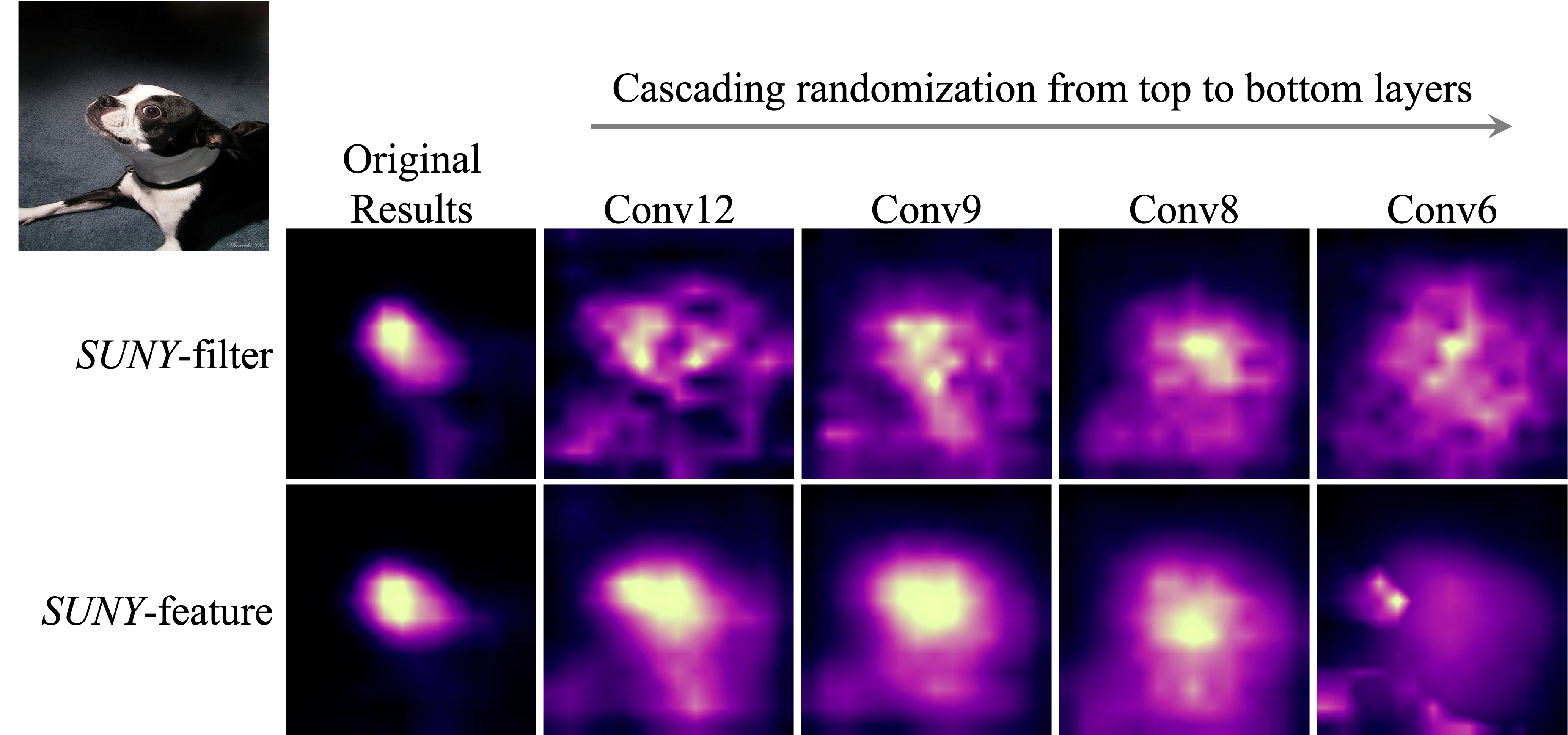
Figure 6: Sanity check of SUNY explanations for VGG16 by cascading randomization with an example image (shown on the top left) from ILSVRC. Results of SUNY-filter and SUNY-feature are represented in the first and second row, respectively. The first column is the original saliency maps, and the following columns show results after randomizing specific layers.

5.6 Sanity Check

The sanity check [2] is to validate whether a visual explanation method can be considered as a reliable explanation to reflect the model’s behavior. We conduct cascading randomization to the model’s weights from the top to the bottom layer successively and generate explanations every time after the randomization. If the saliency maps remain similar for the resulting model with widely differing parameters, it means the method fails the sanity check. Fig. 6 presents the sanity check of SUNY-filter and SUNY-feature, which indicates significant changes for both explanation results after the model parameter randomization. Therefore, the explanations provided by SUNY pass the sanity check.

6 Conclusion

We design a causality-driven framework, SUNY, for bi-directional CNN interpretation from a necessary and sufficient perspective. By establishing a causal mechanism for the CNN classification process, we conduct causal analysis by regarding the CNN model’s prediction probability of a target class as the outcome and the model filters or input features as the hypothesized causes, respectively. Furthermore, our explanations, SUNY-filter and SUNY-feature, are provided by 2D saliency maps, a unique visual explanation design to support a more informative model interpretation. Our semantic evaluation results show that SUNY can provide more insightful visualizations and demonstrate how model interpretations can benefit from necessity and sufficiency information. Moreover, SUNY explanations also pass the sanity check and quantitatively outperform seven other visual explanation methods in necessity and sufficiency evaluation, saliency attack, and localization evaluations using two different large-scale public datasets for two CNN models.

In the future, we plan to exploit the generality of SUNY framework in the scenario of interpreting image segmentation and vision-language tasks. In addition, we plan to apply SUNY in data and model validation.

References

- [1] Kjersti Aas, Martin Jullum, and Anders Løland. Explaining individual predictions when features are dependent: More accurate approximations to shapley values. Artificial Intelligence, 298:103502, 2021.
- [2] Julius Adebayo, Justin Gilmer, Michael Muelly, Ian Goodfellow, Moritz Hardt, and Been Kim. Sanity checks for saliency maps. arXiv preprint arXiv:1810.03292, 2018.
- [3] Christel Baier, Clemens Dubslaff, Florian Funke, Simon Jantsch, Rupak Majumdar, Jakob Piribauer, and Robin Ziemek. From verification to causality-based explications. arXiv preprint arXiv:2105.09533, 2021.
- [4] Aditya Chattopadhay, Anirban Sarkar, Prantik Howlader, and Vineeth N Balasubramanian. Grad-CAM++: Generalized gradient-based visual explanations for deep convolutional networks. In 2018 IEEE Winter Conference on Applications of Computer Vision (WACV), pages 839–847. IEEE, 2018.
- [5] Aditya Chattopadhyay, Piyushi Manupriya, Anirban Sarkar, and Vineeth N Balasubramanian. Neural network attributions: A causal perspective. In International Conference on Machine Learning, pages 981–990. PMLR, 2019.
- [6] Hana Chockler and Joseph Y Halpern. Responsibility and blame: A structural-model approach. Journal of Artificial Intelligence Research, 22:93–115, 2004.
- [7] Zeyu Dai, Shengcai Liu, Ke Tang, and Qing Li. Saliency attack: Towards imperceptible black-box adversarial attack. arXiv preprint arXiv:2206.01898, 2022.
- [8] Anupam Datta, Shayak Sen, and Yair Zick. Algorithmic transparency via quantitative input influence: Theory and experiments with learning systems. In 2016 IEEE symposium on security and privacy (SP), pages 598–617. IEEE, 2016.
- [9] Hichem Debbi. Causal explanation of convolutional neural networks. In Joint European Conference on Machine Learning and Knowledge Discovery in Databases, pages 633–649. Springer, 2021.
- [10] Xiaoyi Dong, Jiangfan Han, Dongdong Chen, Jiayang Liu, Huanyu Bian, Zehua Ma, Hongsheng Li, Xiaogang Wang, Weiming Zhang, and Nenghai Yu. Robust superpixel-guided attentional adversarial attack. In Proceedings of the IEEE/CVF Conference on Computer Vision and Pattern Recognition, pages 12895–12904, 2020.
- [11] Tulia G Falleti and Julia F Lynch. Context and causal mechanisms in political analysis. Comparative political studies, 42(9):1143–1166, 2009.
- [12] Amirata Ghorbani, Abubakar Abid, and James Zou. Interpretation of neural networks is fragile. In Proceedings of the AAAI conference on artificial intelligence, volume 33, pages 3681–3688, 2019.
- [13] Madelyn Glymour, Judea Pearl, and Nicholas P Jewell. Causal inference in statistics: A primer. John Wiley & Sons, 2016.
- [14] Guy Grinfeld, David Lagnado, Tobias Gerstenberg, James F Woodward, and Marius Usher. Causal responsibility and robust causation. Frontiers in Psychology, 11:1069, 2020.
- [15] David Gunning. Explainable artificial intelligence (xai). Defense Advanced Research Projects Agency (DARPA), nd Web, 2, 2017.
- [16] Joseph Y Halpern and Judea Pearl. Causes and explanations: A structural-model approach. part i: Causes. The British journal for the philosophy of science, 2020.
- [17] Michael Harradon, Jeff Druce, and Brian Ruttenberg. Causal learning and explanation of deep neural networks via autoencoded activations. arXiv preprint arXiv:1802.00541, 2018.
- [18] Maksims Ivanovs, Roberts Kadikis, and Kaspars Ozols. Perturbation-based methods for explaining deep neural networks: A survey. Pattern Recognition Letters, 150:228–234, 2021.
- [19] Ramaravind Kommiya Mothilal, Divyat Mahajan, Chenhao Tan, and Amit Sharma. Towards unifying feature attribution and counterfactual explanations: Different means to the same end. In Proceedings of the 2021 AAAI/ACM Conference on AI, Ethics, and Society, pages 652–663, 2021.
- [20] David A Lagnado, Tobias Gerstenberg, and Ro’i Zultan. Causal responsibility and counterfactuals. Cognitive science, 37(6):1036–1073, 2013.
- [21] Peter Lipton. Contrastive explanation. Royal Institute of Philosophy Supplements, 27:247–266, 1990.
- [22] Scott M Lundberg and Su-In Lee. A unified approach to interpreting model predictions. Advances in neural information processing systems, 30, 2017.
- [23] Sébastien Marcel and Yann Rodriguez. Torchvision the machine-vision package of torch. In Proceedings of the 18th ACM international conference on Multimedia, pages 1485–1488, 2010.
- [24] Tanmayee Narendra, Anush Sankaran, Deepak Vijaykeerthy, and Senthil Mani. Explaining deep learning models using causal inference. arXiv preprint arXiv:1811.04376, 2018.
- [25] Daniel Omeiza, Skyler Speakman, Celia Cintas, and Komminist Weldermariam. Smooth Grad-CAM++: An enhanced inference level visualization technique for deep convolutional neural network models. arXiv preprint arXiv:1908.01224, 2019.
- [26] Adam Paszke, Sam Gross, Soumith Chintala, Gregory Chanan, Edward Yang, Zachary DeVito, Zeming Lin, Alban Desmaison, Luca Antiga, and Adam Lerer. Automatic differentiation in pytorch. 2017.
- [27] Judea Pearl. Causality. Cambridge university press, 2009.
- [28] Vitali Petsiuk, Abir Das, and Kate Saenko. Rise: Randomized input sampling for explanation of black-box models. arXiv preprint arXiv:1806.07421, 2018.
- [29] Marco Tulio Ribeiro, Sameer Singh, and Carlos Guestrin. ” why should i trust you?” explaining the predictions of any classifier. In Proceedings of the 22nd ACM SIGKDD international conference on knowledge discovery and data mining, pages 1135–1144, 2016.
- [30] Olga Russakovsky, Jia Deng, Hao Su, Jonathan Krause, Sanjeev Satheesh, Sean Ma, Zhiheng Huang, Andrej Karpathy, Aditya Khosla, Michael Bernstein, Alexander C. Berg, and Li Fei-Fei. ImageNet Large Scale Visual Recognition Challenge. International Journal of Computer Vision (IJCV), 115(3):211–252, 2015.
- [31] Ramprasaath R Selvaraju, Michael Cogswell, Abhishek Das, Ramakrishna Vedantam, Devi Parikh, and Dhruv Batra. Grad-CAM: Visual explanations from deep networks via gradient-based localization. In Proceedings of the IEEE international conference on computer vision, pages 618–626, 2017.
- [32] Karen Simonyan and Andrew Zisserman. Very deep convolutional networks for large-scale image recognition. arXiv preprint arXiv:1409.1556, 2014.
- [33] Daniel Smilkov, Nikhil Thorat, Been Kim, Fernanda Viégas, and Martin Wattenberg. Smoothgrad: removing noise by adding noise. arXiv preprint arXiv:1706.03825, 2017.
- [34] Erik Štrumbelj and Igor Kononenko. Explaining prediction models and individual predictions with feature contributions. Knowledge and information systems, 41(3):647–665, 2014.
- [35] Mukund Sundararajan and Amir Najmi. The many shapley values for model explanation. In International conference on machine learning, pages 9269–9278. PMLR, 2020.
- [36] Christian Szegedy, Vincent Vanhoucke, Sergey Ioffe, Jon Shlens, and Zbigniew Wojna. Rethinking the inception architecture for computer vision. In Proceedings of the IEEE conference on computer vision and pattern recognition, pages 2818–2826, 2016.
- [37] Haofan Wang, Mengnan Du, Fan Yang, and Zijian Zhang. Score-CAM: Improved visual explanations via score-weighted class activation mapping. arXiv preprint arXiv:1910.01279, 2019.
- [38] Jie Wang, Zhaoxia Yin, Jing Jiang, and Yang Du. Attention-guided black-box adversarial attacks with large-scale multiobjective evolutionary optimization. International Journal of Intelligent Systems, 2022.
- [39] David S Watson, Limor Gultchin, Ankur Taly, and Luciano Floridi. Local explanations via necessity and sufficiency: Unifying theory and practice. In Uncertainty in Artificial Intelligence, pages 1382–1392. PMLR, 2021.
- [40] Peter Welinder, Steve Branson, Takeshi Mita, Catherine Wah, Florian Schroff, Serge Belongie, and Pietro Perona. Caltech-ucsd birds 200. 2010.
- [41] Wikipedia contributors. Taxonomic rank — Wikipedia, the free encyclopedia, 2022. [Online; accessed 19-October-2022].
- [42] James Woodward. Sensitive and insensitive causation. The Philosophical Review, 115(1):1–50, 2006.
- [43] Tao Xiang, Hangcheng Liu, Shangwei Guo, Tianwei Zhang, and Xiaofeng Liao. Local black-box adversarial attacks: A query efficient approach. arXiv preprint arXiv:2101.01032, 2021.
- [44] Liuyi Yao, Zhixuan Chu, Sheng Li, Yaliang Li, Jing Gao, and Aidong Zhang. A survey on causal inference. ACM Transactions on Knowledge Discovery from Data (TKDD), 15(5):1–46, 2021.
- [45] Matthew D Zeiler and Rob Fergus. Visualizing and understanding convolutional networks. In European conference on computer vision, pages 818–833. Springer, 2014.
- [46] Qinglong Zhang, Lu Rao, and Yubin Yang. Group-cam: group score-weighted visual explanations for deep convolutional networks. arXiv preprint arXiv:2103.13859, 2021.
- [47] Bolei Zhou, Aditya Khosla, Agata Lapedriza, Aude Oliva, and Antonio Torralba. Learning deep features for discriminative localization. In Proceedings of the IEEE conference on computer vision and pattern recognition, pages 2921–2929, 2016.