Convolutional Visual Prompts for Self-Supervised Adaptation on Out-of-Distribution Data

Convolutional Visual Prompt
for Robust Visual Perception

Abstract

Vision models are often vulnerable to out-of-distribution (OOD) samples, which often need adaptation to fix them. While visual prompts offer a lightweight method of input-space adaptation for large-scale vision models, they rely on a high-dimensional additive vector and labeled data. This leads to overfitting when adapting models in a self-supervised test-time setting without labels. We introduce convolutional visual prompts (CVP) for label-free test-time adaptation for robust visual perception. The structured nature of CVP demands fewer trainable parameters, less than 1% compared to standard visual prompts, combating overfitting. Extensive experiments and analysis on a wide variety of OOD visual perception tasks show that our approach is effective, improving robustness by up to 5.87% over several large-scale models.

1 Introduction

Deep models surpass humans when tested on in-distribution data, yet their performance plummets when encountering unforeseen out-of-distribution (OOD) data at test time, such as unexpected corruptions and shiftings [20, 22, 21, 18, 44]. This vulnerability raises serious risks when these models are deployed, especially in safety-critical applications and high-stakes tasks [49]. Prior works have studied how to improve generalization to OOD data at training time [54, 38, 56, 12, 36, 35, 39, 31], yet little work has been done to adapt the model to OOD at test time, and most of them require to modify model weights [59, 71, 55, 33].

Visual prompting emerges as an efficient and lightweight method to adapt the model at test time without modifying the model [11, 60, 1] (previously also called adversarial reprogramming). In contrast to finetuning the whole model weights, prompting can modify the original task of the model by providing context in the input space. It requires fewer OOD samples and simplifies model version management for practical applications. However, the OOD samples must be labeled, preventing these methods from combating unforeseen distribution shifts.

Recent work [40] defends against unseen attacks at test time by repairing the adversarial inputs with "reversal vectors" – high-dimensional prompt vectors directly added to inputs. It generates the prompts by minimizing a self-supervised loss, requiring no prior labeled OOD samples. Unlike adversarial attacks that damage arbitrary pixels by arbitrary amounts (within a given bound), however, structured changes known as visual distribution shifts are not effectively addressed by unstructured high dimensional vector prompts. Given that a self-supervised objective often has a shortcut and trivial solutions [13], we empirically find prompts without the right structures often improve performance minimally. (Sec. 5.2).

This paper presents Convolutional Visual Prompt (CVP), which uses the convolutional structure as an inductive bias for adapting to visual OOD samples at test time. Prior work has demonstrated that convolutional operations are effective for handling structured data with local motifs [30, 64]. Inspired by this, CVPs are convolutional kernels with only a small number of tunable parameters – less than 1% of the number of tunable parameters in typical unstructured visual prompts (see Figure 1 for illustration), making CVP extremely lightweight and efficient to adapt.

figurec

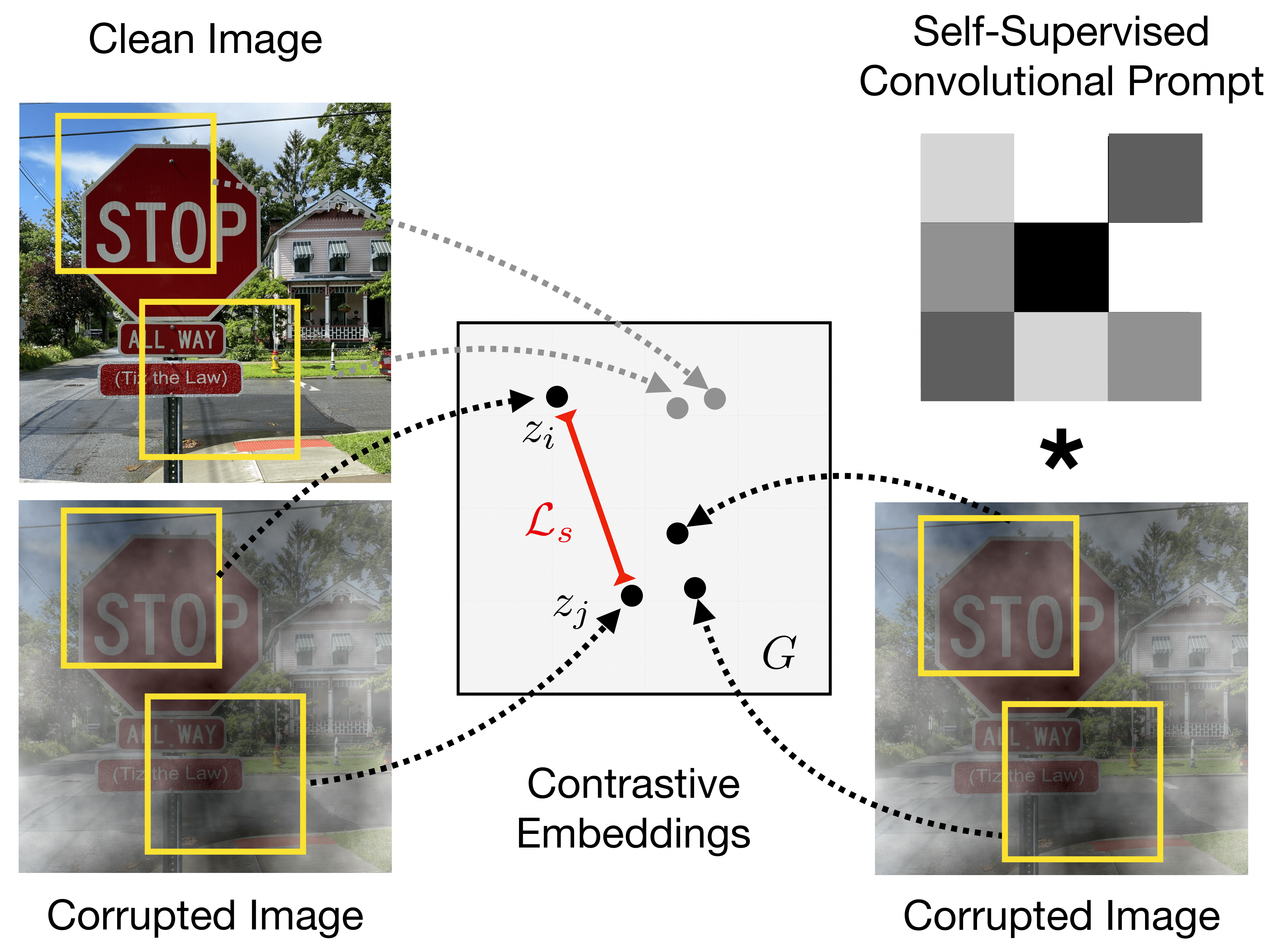
Figure 1: We demonstrate the self-supervised convolutional prompt that adapts model for robust perception. Clean image has a low self-supervision loss, denoted by the distance $\mathcal{L}_{s}$ on the contrastive embedding. When an image is corrupted (e.g, a stop sign in foggy weather), the self-supervised loss generally increases. We then apply the convolutional visual prompts on the corrupted samples, which instruct the model to adapt and produce a small self-supervision loss.

Our experiments show the importance of structured inductive bias for self-supervised adaptation: compared to high-dimensional free-form visual prompts, standard low-rank structured prompts improve robustness by 3.38%, and convolutional structure in prompts is significantly better than low-rank prompts by 2.94% on CIFAR-10-C. On ImageNet-Rendition, ImageNet-Sketch, and 15 types of unforeseen corruptions for both CIFAR-10 and ImageNet at five different severity levels, CVP improves robustness by 5.87% for popular large-scale visual models, including ResNet50, WideResNet18, and the state-of-the-art vision-language model CLIP [51]. Since our method modifies the input space, it complements established test-time model weight adaptation methods (e.g., TENT [62], BN [55], and MEMO [71]) and can be generalized to multiple self-supervised objectives, such as contrastive learning [4], rotation [14], and masked autoencoder (MAE) [15].

2 Related Work

Domain Generalization.

OOD data can lead to a severe drop in performance for machine learning models [20, 18, 53, 44, 39, 42]. Domain generalization (DG) aims at adapting the model with OOD samples without knowing the target domain data during training time. Adapting the model on OOD data [74, 10, 32, 73, 71, 55, 39, 42, 62, 59] also improves robustness.

Test-time adaptation is a new paradigm for robustness against distribution shift [40, 59, 71], mostly updating the weights of deep models. BN [55, 33] updates the model using batch normalization statistics, TENT [59] adapts the model weight by minimizing the conditional entropy on every batch. TTT [59] attempts to train the model with an auxiliary self-supervision model for rotation prediction and utilize the SSL loss to adapt the model. MEMO [71] augments a single sample and adapts the model with the marginal entropy of the augmented samples. Test time transformation ensembling (TTE)  [50] proposes to augment the image with a fixed set of transformations and ensembles the outputs through averaging. The only two works that do not update the models is [40, 45], which modifies the pixels of adversarial, not OOD, samples to minimize the self-supervised objective.

Visual Prompting.

Prompting was proposed in the natural language processing field to provide context to adapt the model for specific tasks [2]. Leveraging this idea, visual prompts [68, 26] adapt the model with a small number of trainable parameters in input space for vision tasks [9, 43] and foundation models [51]. Others proposed to prompt the samples with adversarial perturbations to repurpose the model for target classification tasks, known as adversarial reprogramming [11, 27, 60, 66], sharing the same idea with Visual Prompting. Black-box adversarial reprogramming [60] reprograms a black-box model for downstream classification tasks with limited data. V2S [66] reprograms speech recognition model for time-series data classification tasks. Robust visual prompts [41] are tuned at training time to improve the adversarial robustness of the model under attack. However, this work has not yet been applied to domain generalization where distribution is naturally shifted.

Self-supervised learning (SSL).

SSL can learn effective representations from images without annotations [7, 6, 3, 22]. Prior works have shown that representations learned from different pretext tasks (jigsaw puzzles [47], rotation prediction [14], image colorization [29] and deep clustering [25], etc.) can be leveraged for several downstream tasks such as image classification [4], object detection [8] and test-time domain adaptation [58]. Another well-known branch of SSL is contrastive learning, which aims at grouping associated features for a transformation of samples and distancing from other samples with dissimilar features in the dataset [5, 16, 48]. Some of the methods  [22, 57, 70] use SSL for outlier detection, which aims to learn generalizable out-of-distribution features and rejects them during the testing time. In contrast to these methods which require information from the targeted domain distribution during the training phase for adaptation, our method can adapt the model without requiring any information on unforeseen domains during the testing phase.

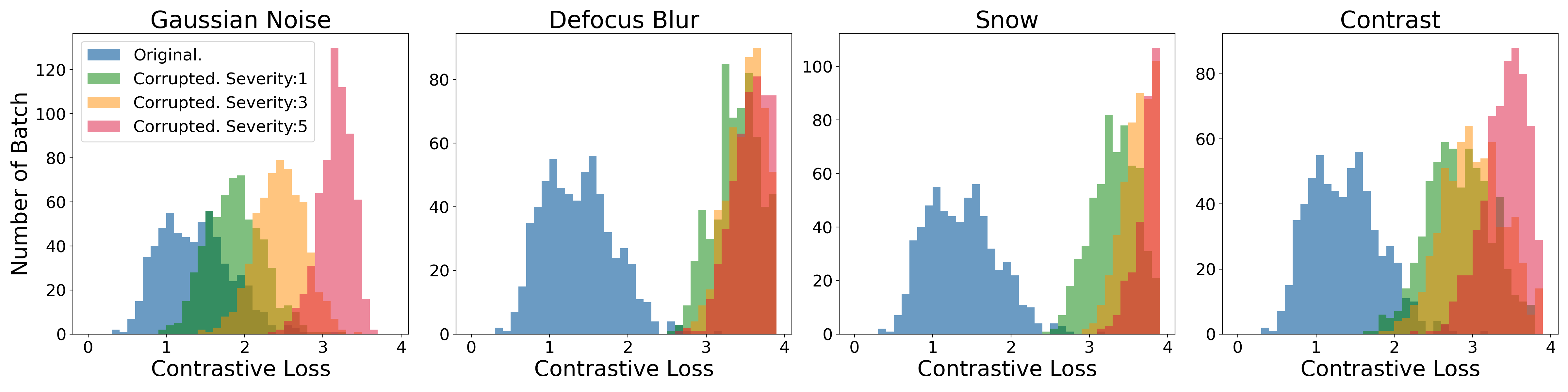
Figure 2: We show the histogram of the contrastive loss distribution on different corruption types. The blue region represents the loss distribution of original sample. The yellow, green, and red regions represent the loss distribution of corrupted samples with different severity (1, 3, and 5). Our plot shows the great shifting in SSL loss distribution between original and corrupted samples.

3 Test-Time Convolutional Visual Prompting

3.1 Learning Intrinsic Structure with Self-Supervision Task

Standard ways to improve model robustness on OOD data is through making the training robust, where the training algorithm anticipates possible corruptions and distribution shifts at inference time and trains on them [18]. However, anticipating the test-time shifting is a strong assumption which is often unrealistic in the real world. Therefore, we improve robustness at test time by dynamically adapting to unforeseen corruptions and unknown shifts.

The ideal case of adapting the model at inference time is to know the ground truth label for the target task, yet this is impossible given that the test data is not labeled. To significantly improve performance on the downstream classification tasks for unlabeled data, we must choose the right self-supervision task that shares rich information with the target classification task.

There is a large body of work on good self-supervision tasks for representation learning at training time. For example, jigsaw puzzles [47], rotation prediction [14], image colorization [29] and deep clustering [25] can be applied to several downstream tasks such as image classification [4], object detection [8] and test-time domain adaptation [58].

For visual recognition, a popular self-supervised objective is contrastive learning, which learns a representation that maps the feature of the transformations of the same image into a nearby place. This is formally defined as:

$$\mathcal{L}_{s}(x)=-\mathbb{E}_{i,j}\left[y_{i,j}^{s}\log\frac{\exp(\cos(z_{i},z_{j}))/\tau}{\sum_{k}\exp(\cos(z_{i},z_{k}))/\tau}\right],$$ (1)

where $z$ are the contrastive features of $x$ extracted from pre-trained backbone. $y_{i,j}^{s}$ is a 0-1 vector for indicating the positive pairs and negative pairs. If $y_{i,j}^{s}$ is 1, the $i$-th feature $z_{i}$ and $j$-th feature $z_{j}$ are both from the $x$ sample. Otherwise, they are from different $x$. We denote $\cos(\cdot,\cdot)$ the cosine similarity, $\tau$ as temperature scaling value. We optimize the model parameters for SSL model $\mathcal{C}$ by using the contrastive loss. The objective function for training is defined as $\min_{\theta_{\mathcal{C}}}\mathop{\mathbb{E}}_{(x)\sim\mathcal{X}_{s}}\big{[}\mathcal{L}_{s}(\cdot)\big{]}$, where $\mathcal{X}_{s}$ is the source domain data for training. We train only on the clean samples drawn from the non-corrupted dataset. We compare this task to other self-supervision tasks in our ablation study.

Since we need to train the self-supervised task at training time, the self-supervised task will perform high on the test data that is the same distribution as the training one. Our results find that the performance of the self-supervised task drops largely when the distribution is shifted at test time. See Figure 2. This suggests that the information that is useful for the self-supervised task is collaterally corrupted in addition to the classification performance drop.

Prior work demonstrated significant mutual information between self-supervised tasks and perception tasks, where pretraining with the self-supervised task improves the perception tasks’ performance [7, 6, 3, 22]. We propose to adapt the model to minimize the self-supervised loss at inference time, where self-supervised task is a proxy that captures a large portion of information from the perception task. In recovering the information of the self-supervised tasks, we could recover the information of perception tasks that was corrupted due to distribution shifts.

3.2 Test-time Adaptation for Vision Models

Inference time adaptation allows the model to adapt to the unique characteristics of the new distribution online. However, the key challenge is that the SSL objective we use to adapt the model is a proxy, where there is often a trivial solution that reduces the loss but adapts the model in the wrong way. Several established methods exist to adapt the vision models, including foundation models.

Finetuning (FT) is a standard way to adapt the deep model. It often optimizes all the parameters of the deep models or partially, which is often heavy and requires large space to save the copy of the model to re-initialize and update. Prior work shows that this method is effective when it is finetuned on supervised tasks, yet adapting with the self-supervised task on a few examples remains under-explored. We discuss the finetuning method using the self-supervised task.

Partial Finetuning (PFT) is another way to adapt the model at inference time by only changing the statistics of the batch-normalization layer. This method assumes that the distribution drifts in the mean and standard deviation of the test data and can be recovered through test-time adaptation. The closest existing works are BN [55], Tent [62] and MEMO [71]. Tent updates the BN statistics but needs to continue training on the same distribution. MEMO only requires a single test data point, yet the algorithm is slow due to the whole model update and heavy augmentations. Here, we adapt batch normalization through our proposed contrastive learning-based self-supervised loss.

Visual Prompts (VP) have emerged as a lightweight way to adapt pre-trained models. There are two major ways to apply visual prompts to the vision model. Let the image be ${\bf x}$, it adds a vector ${\bf v}$ to the input image: ${\bf x}={\bf x}+{\bf v}$. For low-rank visual prompts [24, 67], we use a low-rank matrix in $v$ during optimization. Most visual prompts are studied in training setup, yet they are under-explored at inference time. [40, 45] optimize an additive visual prompt on the image to repair the adversarial perturbation and improve the model robustness.

3.3 Adapting via Convolutional Visual Prompts

Adding the right structure is an effective way to avoid trivial solution to the self-supervised objective. We now introduce the convolution visual prompts (CVP), which instruct the deep model to adapt to the test distribution through convolution. Convolution has been proved to be a successful inductive bias for visual tasks [28], which is more sample efficient [34]. Our assumption is that a large family of distribution shifts in the image data are visually structured, which can be modeled by convolution. Our prompt is simple and is defined as:

$${\bf x}={\bf x}+\lambda\text{conv}({\bf x},{\bf k})$$ (2)

One major advantage of the convolution prompt is that the number of parameters in the prompt is significantly lower (1%) than other conventional prompts (e.g., patch prompt and padding prompt). Compared to adapting the whole model weights, our method is light weight and is fast by exploiting the structure of visual distribution shifts In Appendix 7.2, we show the detailed algorithm of CVP. Our lightweight adjustment allows the model to quickly update to the novel data points without too much computation and memory overhead. As vision models are continuously deployed in edge devices, this is extremely important, given the limited computational resources.

4 Experiment

This section demonstrates the detail of experiment settings and evaluates the performance of our method CVP, compared with conventional Visual Prompts (VP) and existing test-time approaches. More analysis are shown in Section 5 and Appendix. We do a comprehensive study on the CVP, including different prompts design, kernel v.s. structure analysis, multiple SSL tasks, sensitivity analysis on the batch size and adapt iterations, GradCam visualization, and optimization cost of CVP.

4.1 Experiment Setting

Dataset. We evaluate our method on five kinds of OOD datasets, including CIFAR-10-C [21], ImageNet-C [46], ImageNet-R [19], ImageNet-Sketch [65], and ImageNet-A [23]. The following describes the details of all datasets.

$\bullet$ Synthetic OOD Data. The corruption data are synthesized with different types of transformations (e.g., snow, brightness, contrast) to simulate real-world corruption. The dataset contains CIFAR-10-C and ImageNet-C. Both of them are the corrupted versions of their original dataset, including 15 corruption types and 5 severity levels. A larger severity level means more corruption is added to the data. To well evaluate our method, We generate the corruption samples with five severities based on the official GitHub code for each 15 corruption types.

$\bullet$ Natural OOD Data. The ImageNet-Rendition [18] contains 30000 images collected from Flickr with specific types of ImageNet’s 200 object classes. ImageNet-Sketch [65] data set consists of 50000 sketch images. The ImageNet-Adversarial [23] is a natural adversarial shifting dataset contains 7500 images collected from the natural world.

Model.

The backbone model architecture is pretrained on WideResNet18 [69] and ResNet26 [17] for CIFAR-10-C, ResNet50 [17] for ImageNet-C, Rendition, and Sketch. We extract the logit features before the fully connected layer of the backbone model for training the SSL model. The SSL model is a simple MLP with the final layer outputting the one-dimensional features for the contrastive learning task. We further extend our prompt method to the foundation model CLIP [51], where we only prompt the vision encoder.

Baseline Details

We compare several test-time adaptation benchmarks with CVP.

$\bullet$ Standard: The baseline uses the pre-trained model without adaptation. For CIFAR-10-C, the standard is trained with 50000 clean CIFAR-10 train dataset on WideResNet18 and ResNet. For ImageNet1K-C, the standard is trained with $\sim$1.2M clean ImageNet train dataset on ResNet50.

$\bullet$ Finetune (FT): We adjust the whole model weight for every upcoming batch during the inference time with the self-supervised loss. In our experiments, after one-batch fine-tuning, the model will be restored to the initial weight status and receive a new type of corrupted samples.

$\bullet$ Partial Finetune (PFT): The partial fine-tune adapts batches of the samples to the model by only adjusting the batch normalization layers with self-supervised loss at every inference time. Same as Finetune baseline, the model will be restored to the initial weight status after the one-batch adaptation.

$\bullet$ SVP [40]: The prompting method to reverse the adversarial attacks by modifying adversarial samples with $\ell_{p}$-norm perturbations, where the perturbations are also optimized via contrastive loss. We extend this method with two different prompt settings: patch and padding. For the patch setup, we directly add a full-size patch of perturbation into the input. For the padding setup, we embed a frame of the perturbation outside the input. More baseline detailed are shown in the Appendix 7.3

Design of Convolutional Visual Prompts (CVP)

We prompt the input samples by adding the convolutional kernels. Our kernels can be optimized under several different settings, including 1.) fixed or random kernel initialization 2.) 3*3 or 5*5 kernel sizes. We show a detailed evaluation of all kernel setups in the experimental results. For initialization, we can either random initialize the kernel size $k$ in a uniform distribution or initialize with fixed values. For fixed initialization, we empirically found that starting from a sharpness kernel is effective. We optimize the kernel with 1 to 5 iterations of projected gradient descent. To preserve the original structure, we combine the residual of input and convolved output with learnable parameters $\lambda$. We jointly optimize the convolutional kernel $k$ and $\lambda$ with the self-supervised loss $\mathcal{L}_{s}$. The range of $\lambda$ is predefined and empirically set up in a fixed range. For CIFAR-10-C, we set up the range as [0.5, 3], and for ImageNet-C is set up as [0.5, 1]. We describe the detailed parameter settings and different prompt designs in the Appendix 7.4 7.7.

Method/Model	WideResNet18 Avg. Error (%)	ResNet26 Avg. Error (%)
Standard	58.24	62.12
FT	69.33 (+11.09)	63.07 (+0.95)
PFT	62.65. (+4.41)	62.47 (+0.34)
SVP (patch)	57.94 (-0.3)	62.82 (+0.7)
SVP (padding)	58.20 (-0.04)	62.18 (+0.06)
CVP-F3	53.67 (-4.57)	59.52 (-2.6)
CVP-R3	52.37 (-5.87)	59.32 (-2.80)

Table 1: Corruption benchmarks on CIFAR-10-C. We show the average error rate on 15 corruption types and 5 severities for CVP, compared with the baselines. For the CVP results, we denote the two initialization settings: fixed/random as F / R, and the number behind F / R means the kernel size (e.g., 3 or 5). We set up the batch size of adaption as 16 and the number of adapt iters as 5 for all methods.

	ImageNet-C mCE $\downarrow$	ImageNet-R Error (%)	ImageNet-S Error (%)	ImageNet-A Error (%)
ResNet50	76.87	63.83	75.90	100.0
FT	77.10 (+0.26)	64.38(+0.55)	76.38 (+0.48)	99.95 (-0.05)
PFT	76.74 (-0.13)	69.63 (+5.8)	80.43 (+4.53)	99.89 (-0.11)
SVP (patch)	76.74 (-0.13)	68.86 (+5.03)	75.93 (+0.03)	99.94 (-0.06)
SVP (padding)	80.07 (+3.23)	63.84 (+0.01)	75.92 (+0.02)	99.91 (-0.01)
CVP-F3	75.88 (-0.95)	63.56 (-0.27)	75.32 (-0.58)	99.2 (-0.8)
CVP-R3	75.34 (-1.49)	63.49 (-0.34)	75.30 (-0.60)	99.2 (-0.8)
CVP-F5	75.74 (-1.09)	63.18 (-0.65)	75.35 (-0.55)	98.67 (-1.33)
CVP-R5	75.77(-1.06)	63.06 (-0.77)	75.33 (-0.57)	98.4 (-1.6)

Table 2: Comparison on CVP with other baselines on ImageNet-C, ImageNet-R, ImageNet-S, and ImageNet-A. The standard model is ResNet50 [17]. For ImageNet-C, we calculate the mean corruption error (mCE). Same as Table 1, we evaluate the CVP under multiple kernel setups and show the results. For ImageNet-C and Sketch, CVP-F3 achieves the best robustness, which reduces the error rate by 1.49% and 0.6%. Other datasets, such as ImageNet-R and ImageNet-A, outperform all the baselines when updating 5*5 kernels with random initialization.

	CIFAR-10-C	ImageNet-C	ImageNet-R	ImageNet-S
	Avg. Error (%)	mCE $\downarrow$	Error (%)	Error (%)
CLIP(ViT/32)	58.39	77.93	32.09	60.55
SVP (patch)	58.43 (+0.04)	77.81 (-0.12)	32.12 (+0.03)	60.53 (-0.02)
CVP-F3	57.94 (-0.45)	77.43 (-0.50)	31.16 (-0.93)	59.47 (-1.08)
CVP-R3	57.91 (-0.48)	77.71 (-0.22)	31.31 (-0.78)	59.62 (-0.93)
CVP-F5	57.98(-0.41)	77.25 (-0.68)	31.14 (-0.95)	59.83 (-0.72)
CVP-R5	57.79 (-0.60)	76.67 (-1.26)	30.43 (-1.66)	59.43 (-1.12)

Table 3: Evaluation on the CLIP model. We compare CVP with other prompting baselines on CIFAR-10-C, ImageNet-C, ImageNet-R, and ImageNet-S. Overall, the CVP-R5^† achieves the best performance, which reduces the error rate by 1.16% on average.

4.2 Experimental Results

Table 1 presents the evaluation results of CVP on CIFAR-10-C. We compare CVP with five different baselines, including standard, VP (patch/padding), fine-tune (FT), and partially fine-tune (PFT) with SSL loss, using two model architectures. We also explore different kernel settings of CVP, including fixed/random initialization and different kernel size. Results show that for WideResNet18, CVP achieves the highest reduction in average error rate by 5.87% when updating the 3*3 kernel with random initialization. For ResNet-26, CVP consistently reduces the error rate by 2.8%.

Table 2 displays the results for ImageNet-C, Rendition, Sketch, and Adversarial. The standard baseline is pre-trained on ResNet50 [17]. For ImageNet-C, we report the mean corruption error (mCE), calculated with the performance rates on ResNet50 and standard AlexNet following the benchmark [21]. Due to the larger dimension of the ImageNet dataset (224), a larger kernel size effectively captures more information from the input. Thus, we set the kernel size as 3*3 and 5*5. Our findings indicate that CVP achieves the highest error rate reduction for ImageNet-R and A by 0.77% and 1.6%, respectively, when updating with a 5*5 kernel using random initialization. CVP consistently outperforms all baselines for ImageNet-C and Sketch. We observe that VP (patch) and VP (padding) degrade performance on most datasets, suggesting that unstructured perturbations with more trainable parameters are ineffective in adapting to natural OOD data with general shifts.

In Table 3, we further evaluate the performance of CVP on the large-scale foundation model, CLIP [52]. Compared to the baselines VP (padding) and VP (patch), CVP achieves the best performance on all datasets when updating under random initialization with 5*5 kernel size.

	CIFAR-10-C Avg. Error (%)	ImageNet-C mCE $\downarrow$	ImageNet-R Error (%)	ImageNet-S Error (%)	ImageNet-A Error (%)
Standard	58.24	76.87	63.83	75.90	100.0
Mao et al. [40]	57.94 (-0.3)	76.74 (-0.13)	68.86 (+5.03)	75.93 (+0.03)	99.94 (-0.06)
CVP (ours)	52.37 (-5.87)	75.43 (-1.49)	63.06 (-0.77)	75.30 (-0.6)	98.4 (-1.6)
MEMO [71]	56.14	73.45	60.73	73.43	99.1
MEMO + CVP	54.84 (-1.3)	72.02 (-1.43)	60.23 (-0.5)	72.67 (-0.76)	98.64 (-0.46)
BN [55]	38.51	76.20	67.29	77.98	99.8
BN + CVP	37.39 (-1.12)	76.16 (-0.04)	67.21 (-0.08)	77.92 (-0.06)	98.67 (-1.13)
TENT [62]	38.52	70.45	58.45	73.88	99.7
TENT + CVP	36.69 (-1.83)	70.34 (-0.11)	58.42 (-0.03)	73.83 (-0.05)	98.54 (-1.16)

Table 4: Our prompt method complements other test-time adaptation approaches that update model weight, including MEMO, TENT, and BN. We show complements gain on every baseline when combined with CVP. Here, the Standard for CIFAR-10-C is WideResNet18 and other dataset is ResNet50. For CIFAR-10-C, on top of the TENT [62] method, we achieve the best gain on the performance, which reduces 1.83% error rate.

CVP Complements Other Test-Time Adaptation Methods

Since our method modifies the input space and aligns the representation of adapted samples to the original manifold, it also complements established test-time adaptation approaches which adjusts the model weights. Thus, we combine the CVP with several existing methods, including MEMO [71], BN [55], and TENT [62]. For a fair comparison, we set up the batch size as 16 for all experiments. for the parameter settings, we set the kernel size for CIFAR-10-C as 3x3 and ImageNet-C, R, S, and A as 5x5. The adaptation iterations are all set as 5. In Table 4, we show the results on five benchmarks. For CIFAR-10-C, CVP improves 1.83 points on top of TENT and reduces the error rate by 21.55% compared with the standard one. For the other datasets, CVP achieves the lowest error rate on top of the TENT method. However, the BN method degrades the performance under the small batch setting. Due to the page limit, in Appendix 7.5, we show more evaluations on other benchmark, such as the Cutout-and-Paste data [61] and other baseline Test Time Training (TTT) [59].

5 Ablation Study

Figure 3: The effect of structured prompt for reversing corruption. For the y-axis, we show the $\ell_{2}$ distance between the ground-truth additive corruptions vector $\Delta$ and our prompt reversing vectors $\delta$, where a small distance indicates our reversal is successful. For the x-axis, we show the rank for the prompt matrices and the convolutional kernel. For a convolutional kernel with size $k\times k$, its rank is k. We find a small rank help reverse the noise better. For the same rank, convolution is better than the additive matrix. This demonstrates the effectiveness of our convolution prompt over other low-rank structures in reversing natural corruptions.

Low-Rank Structure to Avoid Shortcut in SSL Objective.

Since SSL objective is a proxy for our visual recognition task, sole minimizing SSL objective can produce a overfitted prompt without much improvement in visual recognition. A typical way to avoid this suboptimal solution is by adding the right inductive bias. For the highly structured visual data, we study the best inductive bias we can add to prevent the shortcut during adaptation.

In addition to convolution, we also investigated the popular low-rank structure [24, 67]. We create visual prompts with low-rank structure (LVP) via singular value decomposition (SVD), and optimize the low-rank matrices using our algorithm (shown in Appendix 7.2). We compare the effectiveness of low-dimensional prompts and convolution on their ability to reverse natural corruptions. In Table 7 and Figure 3, for both LVP and CVP, increasing the prompt’s rank leads to degraded performance in reverse the corruption to produce clean images, where the $\ell_{2}$ norm distance between real shifting and the approximated shifting increase.

	CIFAR-10-C	ImageNet-C	ImageNet-R	ImageNet-S
	Avg. Error	mCE	Error	Error
Standard	58.24	76.87	63.83	75.90
SSL-VP	57.95 (-0.29)	76.74 (-0.13)	68.86 (+5.03)	75.93 (+0.03)
SSL-CVP	52.37 (-5.87)	75.34 (-1.53)	63.06 (-0.77)	75.30 (-0.60)
Sup-VP	42.02 (-16.22)	73.54 (-3.33)	60.17 (-3.66)	73.30 (-2.60)
Sup-CVP	49.59 (-8.65)	74.10 (-2.77)	62.60 (-1.23)	74.14(-1.76)

Table 5: Analysis on the shortcut of SSL. We compare the performance of SSL and supervised learning on VP and CVP for four benchmarks

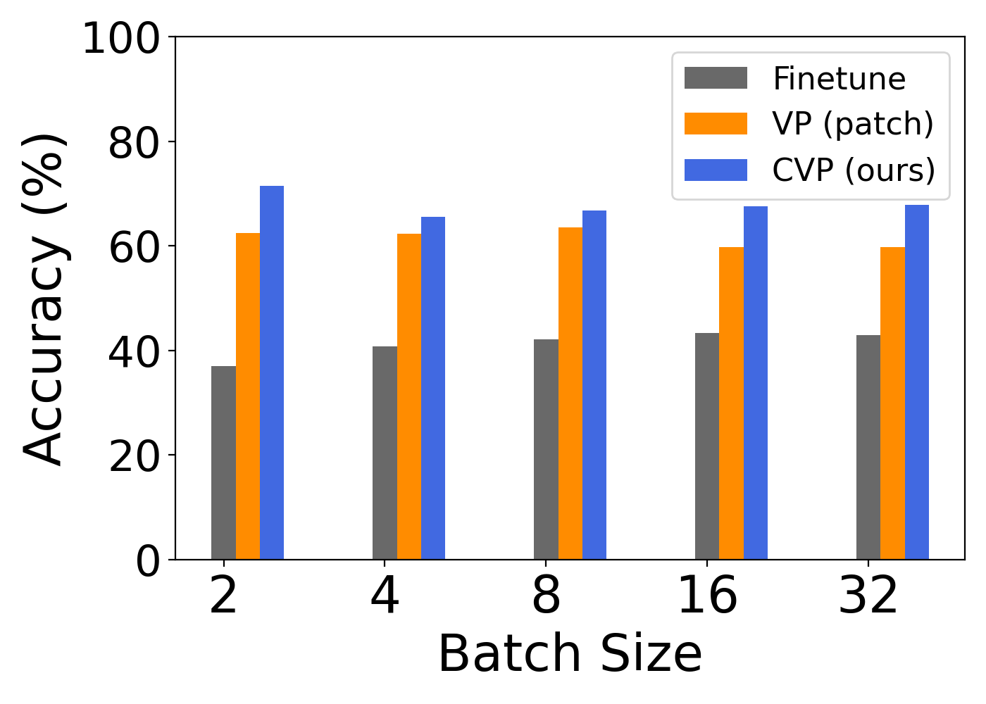
(a)

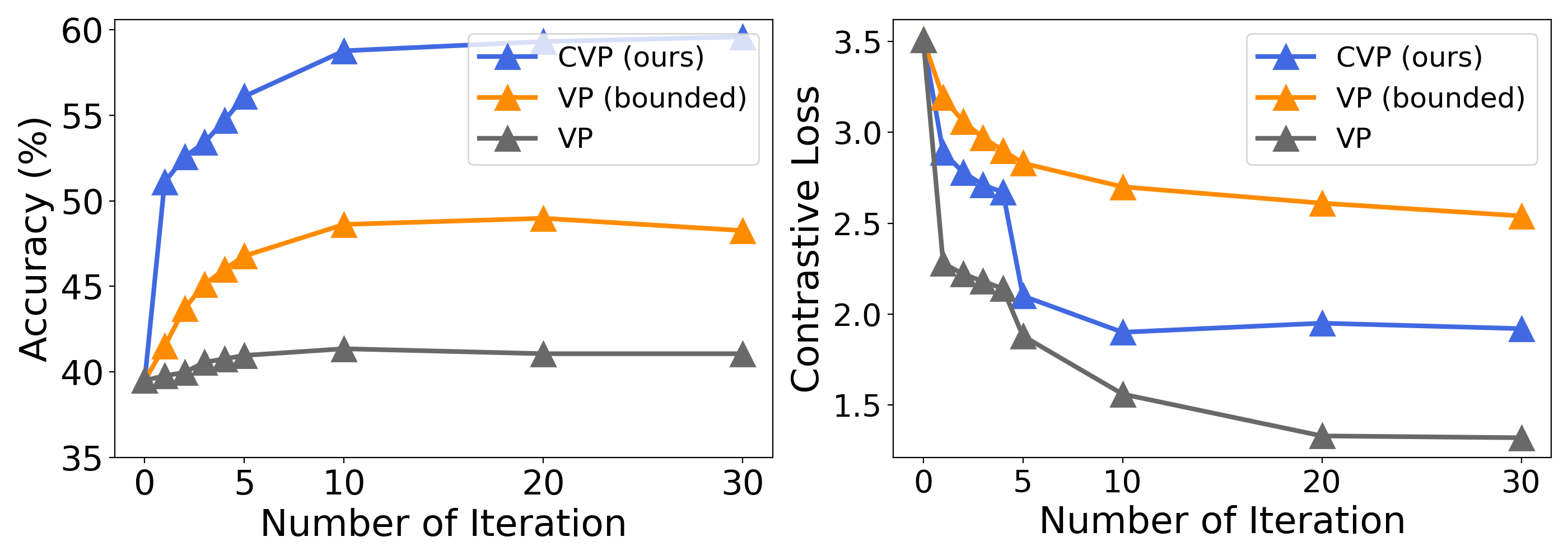
(b)

Figure 4: (a.) Analysis of the effect of batch size for different baselines on Cifar-10-C. We show the average performance on severity 1 for every corruption type. When batch size is small, CVP has a better performance on all corruption types, compared to fine-tune and two VP methods. (b.) We show the analysis for self-supervised loss v.s. performance on VP and CVP for gaussian corruption type in CIFAR-10-C. We setup the norm-bound for VP as 8/255 or unbounded. The loss curve demonstrates that when increasing the iter. number from 1 to 30, adapting with VP without norm bound hugely over-fits the self-supervised loss. The loss of VP largely reduces, yet the performance does not improve. On the other hand, our CVP has a lower risk of over-fitting as the loss curve can reduce smoothly with accuracy gradually increasing.

CVP in Supervised Learning.

CVP is necessary for our test-time adaptation because SSL is a proxy for our final task. There are solutions where SSL is minimized, but the final task performs suboptimal. We investigate the necessity of using CVP when optimized for objectives other than SSL, such as the supervised loss, where the training and evaluation objective matches. Hence, in Table 5, we show the VP and CVP under the supervised learning setting (Sup-VP and Sup-CVP) and SSL setting (SSL-VP and SSL-CVP). For all experiments, we use the same optimization setting and parameter settings as Table 4. We apply the prompts on every batch for the supervised setting and update them with ground truth. Due to training on the ground-truth label, both VP and CVP achieve higher accuracy than SSL, VP performs higher than CVP. The results demonstrate that convolution inductive bias is not necessary when ground truth is available. However, without the label, the structured convolutional prompt is necessary for improving performance.

Standard LVP_R3 CIFAR-10-C 58.24 54.86 (-3.38) ImageNet-C 76.87 76.42 (-0.45) ImageNet-R 63.83 63.57 (-0.26) ImageNet-S 75.90 75.69 (-0.21)

Table 6: Performance of low-rank visual prompt. We show the average error rate on four benchmarks. For CIFAR-10-C, we use WideResnet as the standard model. For ImageNet-C, R, and S, we use the ResNet50.

S1 S2 S3 S4 S5 Standard 58.82 48.25 38.65 27.15 17.57 Contrast 59.53 48.84 39.82 28.55 19.53 Rotation 58.97 48.30 38.88 27.50 17.99 MAE 60.94 51.10 41.79 30.11 19.92

Table 7: Performance of CVP on three SSL tasks for ImageNet-C, including contrastive learning, rotation prediction, and MAE. We compare them with the Standard ResNet50 and show the averaged accuracy for 15 corruption types on every severity.

Generalize CVP to other SSL tasks. We further show the CVP can be generalized to other self-supervision tasks. In Table 7, we compare three SSL tasks, including contrastive learning, rotation prediction and masked autoencoder (MAE) [15]. We show our CVP is effective under all SSL tasks. On ImageNet-C, CVP improves robust accuracy for every severity level (from s1 to s5) when optimized for all three SSL tasks. We find contrastive learning can perform better than rotation prediction, and MAE has the best performance.

The Effect of Batch Size and Number of Iteration for Adaptation. In Figure 4(a), we empirically demonstrate that the batch size affects the performance of different prompt methods. We set up the batch sizes from 2,4,8,16 to 32 and compared the accuracy of CVP with Finetune, VP (padding), and VP (patch). When batch size is set as 2, the performance of fine-tune is only 36.95%, which is worse than CVP (71.53%). When increasing the batch size to 4 and 8, the performance of fine-tune, VP slightly improves, yet still worse than CVP. Overall, CVP has an advantage in adaptation under the small batch setting. In Figure 4(b), we show the performance on different numbers of iterations for adaption. We empirically found that when increasing the iterations, CVP has a lower risk to overfit on the self-supervised objective. More ablation studies, such as different prompt designs can be found in Appendix 7.7

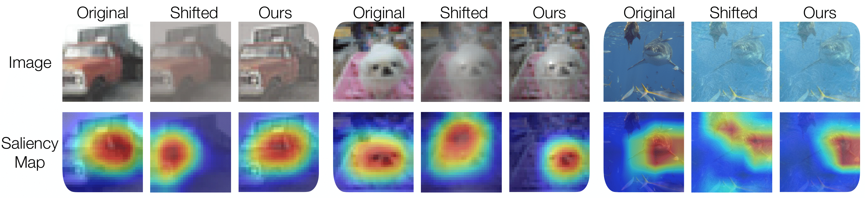
Figure 5: Visualization. From left to right we show three kinds of corruption types, including contrast, fog, and frost, on ImageNet examples. By applying our convolutional prompt on the corrupted images, our method can partially remove the corruptions and make the image easier to recognize. In addition, the saliency map calculated from Grad-Cam also shows that our approach instructs the model to look at a similar region as the original one. This highlights why our convolutional can adapt the input for robustness.

Visualization of Saliency Map To better understand how CVP adapts to the corrupted inputs, we visualize the saliency map of different types of corruption. As Figure 5 shows, from left to right, the first row is the original, corrupted, and adapted samples; the second row shows their corresponding Grad-CAM with respect to the predicted labels. The red region in Grad-CAM highlights where the model focuses on target input. We empirically discover the heap map defocuses on the target object for corrupted samples. After CVP, the red region of the adapted sample’s heap map is re-targeted on a similar part as the original image, demonstrating that the self-supervised visual prompts indeed improve the input adaptation and make the model refocus back on the correct areas. We provide more visualization in Appendix 7.10.

Training Cost v.s. Different Kernel Size In Table 8, we evaluate different kernel sizes for CVP and empirically discover that increasing the kernel to a proper size can improve the performance slightly. We choose one corruption-type impulse noise and show the results. When increasing the kernel size, the optimization cost increases. For impulse noise, kernel size 7*7 achieves the best robust accuracy, yet the optimization cost is much higher.

Kernel Size	Accuracy (%)	Training Cost/Batch
3*3	16.22	0.67s
5*5	16.3	0.68s
7*7	16.62	1.24s
13*13	16.61	1.28s
21*21	16.52	1.29s
25*25	15.4	1.32s

Table 8: Training Cost v.s. Different Kernel Size

Training Time v.s. Number of Adapt Iteration In Figure 4(b), we have shown the CVP trained under different adapt iterations v.s. their performance. When increasing the number of adapt iterations, the training time increases. The following Table 9 shows the result of CIFAR-10-C on gaussian noise type with severity 1. We compare the accuracy and per batch training time on several numbers of adapt iters (from 0 to 20). We empirically found that CVP has a larger performance gain than VP while adapting with a few epochs (epoch number 1).

# of Adapt Iters	0	1	5	10	15	20
Cost/Batch	0.00s	0.17s	0.67s	1.29s	1,.92s	2.57s
CVP Acc.(%)	39.51	51.09	56.1	58.76	59.30	59.58

Table 9: Training Time v.s. Number of Adapt Iteration

Does CVP Reverse Corrupted Images Back to Normal One? We do the quantitative measurement on the distribution distance via Sliced Wasserstein Distance (SWD) and structural similarity index measure (SSIM). We measure the distance between two input distributions: source domain distribution and target domain distribution (before/after CVP adaptation). To calculate the distance between two input distributions via the Sliced Wasserstein Distance, we first obtain a group of marginal distributions from a high dimensional probability distribution via the linear projection, then calculate the $p$-Wasserstein Distance for those marginal distributions. Table 10 and Figure 6 shows the result of SWD on CIFAR-10-C with severity 1. On average, CVP achieves lower SWD after adaptation, which means the target distribution is closer to the source one after adaptation. The average SWD reduce by 0.7% after prompting. In Appendix Table 18 and Figure 9, we show the more detailed analysis.

SWD (scale: $10^{2}$) $\downarrow$ SSIM $\uparrow$ before after before after Avg. Mean 7.19 6.49 0.7539 0.7884 Avg. Std 4.05 2.79 0.1294 0.7260

Table 10: Results of SWD and SSIM on CIFAR-10-C (Severity 1).

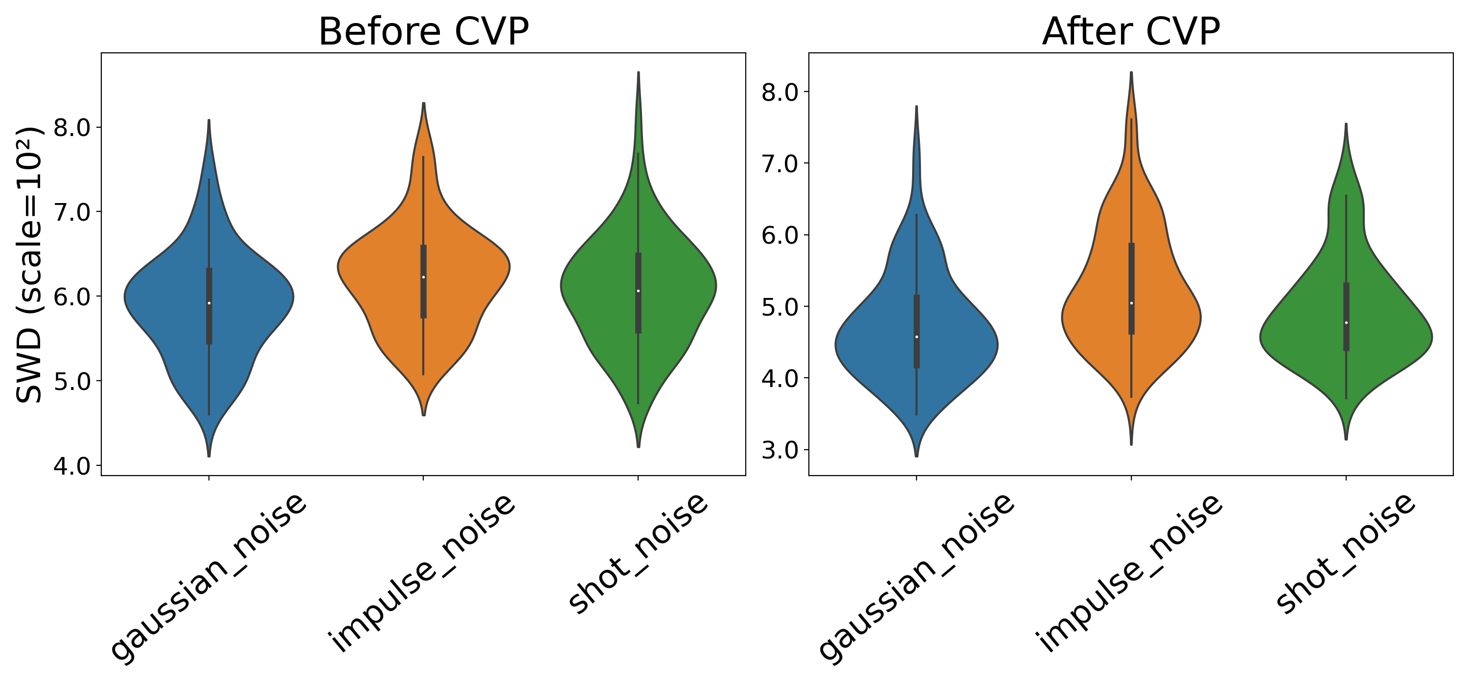
(a) Noise Group

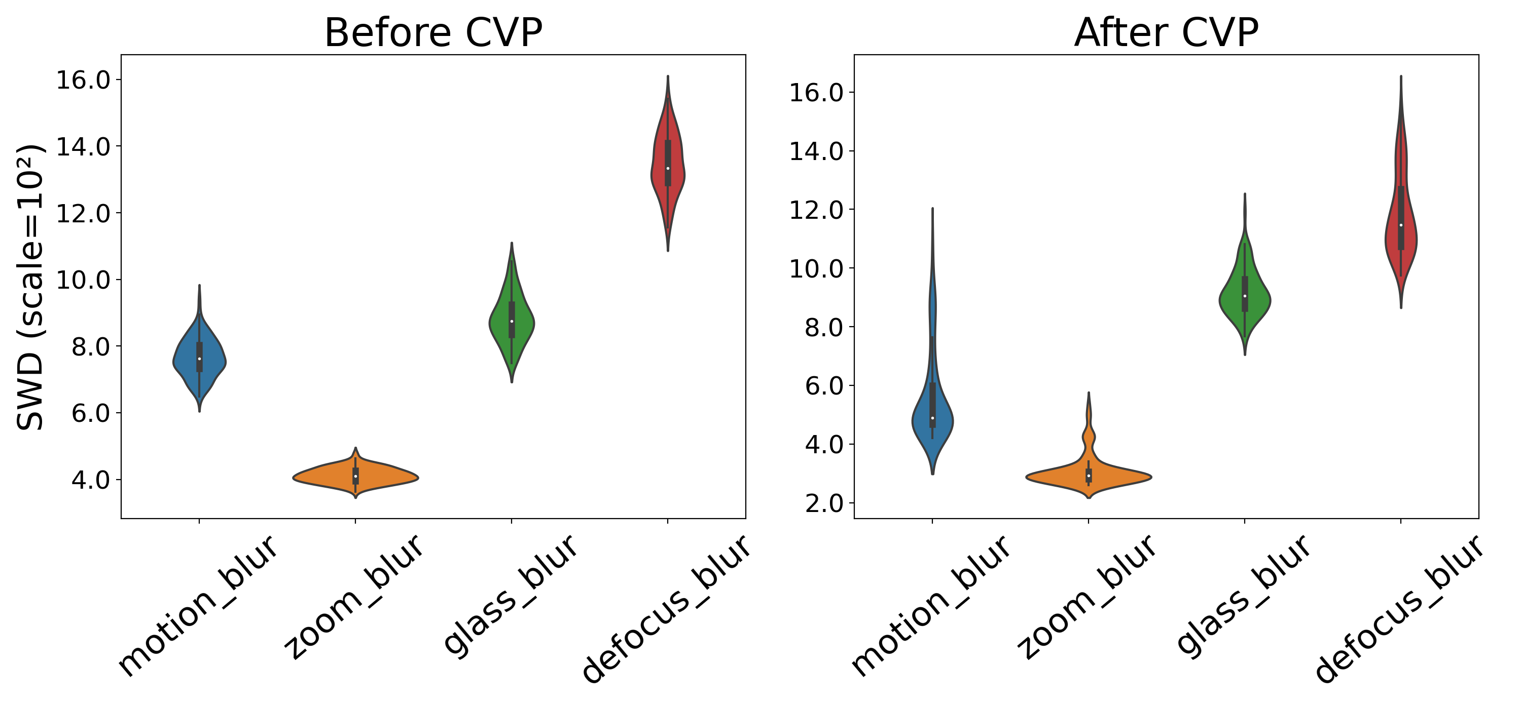
(b) Blur Group

Figure 6: Violin Plot of SWD for different corruption groups on CIFAR-10-C (severity 1). The left figure of each subplot shows the SWD before adapting, and the right shows the SWD after CVP adaptation. CVP brings the corrupted image distribution back to the clean image distribution.

6 Conclusion

Self-supervised convolutional visual prompt (CVP) is a novel method for test-time adaptation of OOD samples. In contrast to prior works training the visual prompts with the label, CVP is label-free and lightweight. It reduces the trainable parameters to less than 1% parameters of previous visual prompts and avoids the risk of overfitting when adapting for self-supervised objectives at test time. Results on five state-of-the-art benchmarks show that CVP improves model robustness by 5.87% and complements existing weight-adaptation methods. Extensive ablation studies suggest that distribution shifts are actually structured; therefore, CVP can capture the structures better than VP during the adaptation, which provides new insight into the frontier of visual prompting techniques and test-time adaptation. Future work includes interpreting convolutional prompts and prompting with multi-modality in large-scale foundation models.

7 Appendix

7.1 Flow of CVP

We illustrate the whole flow of CVP in Figure 7. There are two phases in our proposed method: (1.) Offline one-time training on SSL model: The SSL is a simple MLP model, where it takes the logit features from pre-trained backbone as input and trains the model with contrastive learning task. (2.) CVP adaptation for any OOD benchmark during test time: We leverage the SSL loss from well-trained SSL model to optimize the convolutional kernel prompts for every upcoming OOD sample.

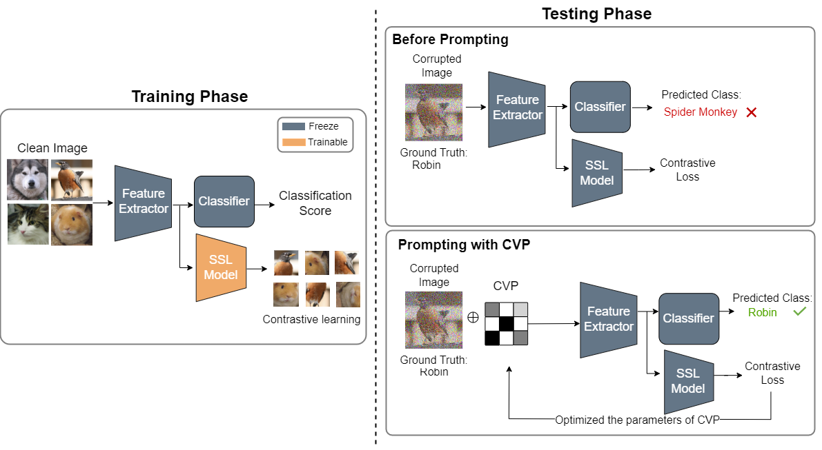
Figure 7:

7.2 Algorithm

Input: Pretrained classifier $\mathcal{F}(\cdot)$, OOD images $x$, Self-supervised objective function $\mathcal{L}_{s}(\cdot)$, Convolutional operator $Conv(\cdot)$, Convolutional kernel $k$, Learning rate $\eta$, Number of iteration $\mathcal{T}$

Output: Class prediction $\hat{y}$ for adapted sample of $x$

1

2Inference

3 # Initialize the kernel parameters

4 $k^{0}\sim\mathcal{U}\{(\alpha,\beta)$

5 # Calculate initial SSL loss

6 $loss^{0}=\mathcal{L}_{s}(x)$

7 for $t\in\{1,...,T\}$ do

8       # Generate adapted samples

9       $x^{t}=x+\lambda*Conv(x,k^{t})$

10       # Calculate SSL loss with adapted samples

11       $loss^{t}=\mathcal{L}_{s}(x^{t})$

12       # Update kernel parameters

13       $k^{t+1}=k^{t}+\eta\frac{\partial loss^{t}}{\partial k^{t}}$

14# Get optimal kernel parameters

15 $k^{\star}\leftarrow k^{T}$

16 if $loss^{T}>loss^{0}$ then

17       # Use the initial kernel parameters

18       $k^{\star}\leftarrow k^{0}$ ;

19      

20 # Get final adapted samples

21 $x^{\star}=x+\lambda*Conv(x,k^{\star})$

return $\hat{y}\leftarrow\mathcal{F}(x^{\star})$

Algorithm 1 Convolutional Visual Prompt

Input: Pretrained classifier $\mathcal{F}(\cdot)$, OOD images $X$, Self-supervised objective function $\mathcal{L}_{s}(\cdot)$, Rank Number $r$, Learning rate $\alpha$, Number of iteration $\mathcal{K}$

Output: Class prediction $\hat{y}$ for adapted sample of $x$

1

2Inference

3 # Initialize the matrices parameters

4 SVD on input $X(N*C*H*W)$ $\rightarrow$ get n pairs of initial $U\Sigma V^{T}$ (3 channel)

5 for $t\in\{1,...,K\}$ do

6       # Get N inverse matrices

7       $M_{t}\leftarrow U_{t}\times\Sigma_{t}\times V^{T}_{t}$

8       # Apply low-rank SVD on $M_{t}$ with rank $r$

9       $U\textquoteright_{t},\Sigma\textquoteright_{t},V^{T^{\prime}}_{t}$ = $SVD_{low-rank}(M_{t})$

10       # Generate adapted samples with low-rank inverse matrices

11       $M\textquoteright_{t}=U\textquoteright_{t}\times\Sigma\textquoteright_{t}\times V^{T^{\prime}}_{t}$

12       $X\textquoteright_{t}=X_{t}+M\textquoteright_{t}$

13       # Calculate SSL loss with adapted samples

14       $loss^{t}=\mathcal{L}_{s}(X^{\prime}_{t})$

15       # Update the three matrices

16       $U_{t+1}=U_{t}+\alpha\frac{\partial loss^{t}}{\partial U_{t}},\quad\Sigma_{t+1}=\Sigma_{t}+\alpha\frac{\partial loss^{t}}{\partial\Sigma_{t}},\quad V^{T}_{t+1}=V^{T}_{t}+\alpha\frac{\partial loss^{t}}{\partial V^{T}_{t}}$

17      

18# Get optimal low rank matrix

19 $M^{\star}\leftarrow U_{K}\times\Sigma_{K}\times V^{T}_{K}$

20 # Get final adapted samples

21 $X^{\star}=X+M^{\star}$

return $\hat{y}\leftarrow\mathcal{F}(X^{\star})$

Algorithm 2 Low-Rank Visual Prompt

7.3 Baseline Details

Here, we show the detail of the baselines that we compare with.

$\bullet$ Standard: The baseline uses pre-trained model without adaptation. For CIFAR-10-C, the standard is trained with 50000 clean CIFAR-10 train dataset on WideResNet18 and ResNet. For ImageNet1K-C, the standard is trained with $\sim$1.2M clean ImageNet train dataset on ResNet50.

$\bullet$ SVP: The self-supervised visual prompts attempt to reverse the adversarial attacks by modifying the input pixels with $\ell_{p}$-norm perturbations, where the perturbations are optimized via contrastive loss [40]. For the patch setting, we setup the shape of VP as 32*32*3 for CIFAR-C and 224*224*3 for all ImageNet OOD datasets. For the padding setting, we set the padding size as 1 for CIFAR-10-C and 15 for ImageNet OOD dataset. Take CIFAR data as example, we first initialize a mask with all zeros value with the shape 30*30*3 and set the pad value as 1 with padding size 1 so that the mask after padding is as the same shape of CIFAR data (32*32*3). Then, we multiply the mask with the VP to preserve only the VP located at the position we just pad with 1 value. We can further optimize the VP with mask by adding it with the corrupted samples.

$\bullet$ BN[55]: The model adaptation method aims to adjust the BN statistics for every input batch during the test-time. It requires to adapt with single corruption type in every batch.

$\bullet$ TTT [59]: The test-time training trains the model with an auxiliary SSL rotation task and leverages the rotation loss for model adaptation during the testing time. In TTT method, instead of adapting the whole model, they only adapt the last few layers of the model and freeze the parameters in the front layers.

$\bullet$ MEMO: The model adaptation method proposed in  [71] alters a single data point with different augmentations (ie., rotation, cropping, and color jitter,…etc), and the model parameters are adapted by minimizing the entropy of the model’s marginal output distribution across those augmented samples.

$\bullet$ TENT [63]: The method adapts the model by minimizing the conditional entropy on batches. In our experiment, we evaluate TENT in $episodic$ mode, which means the model parameter is reset to the initial state after every batch adaptation.

7.4 Implementation details

For the training part of SSL model, we set the training parameters with batch size as 64, training epoch as 200, and the learning rate (lr) as 0.001. The lr is decayed with a cosine annealing for each batch [37]. The transformations for contrastive learning are predefined. We augment the inputs with random resize crop, random flip, and random rotation in degree [-90, 90] for positive/negative pairs generation in every batch. The number of transformations for one sample is set as 3.

For the test-time adaptation part, we set the range of parameter $\delta$ for VP. For the $\ell_{2}$-norm perturbations, the $\epsilon$ is [-8/255,8/255] and the step size is 2/255. We set the iteration number $i$ either as 1 or 5, which means each component has 1 or 5 steps during PGD. For the update iterations, as the Table 17. show a larger number of iterations has better performance. However, the training cost becomes higher.

$\bullet$ The choice of hyper-parameter setting on $\lambda$ ranges and kernel

For the $\lambda$ parameter, it controls the magnitude of convolved output when combined with the residual input. We set the range to be [0.5, 3] and run test-time optimization to automatically find the optimal solution, which does not require a validation set.

We use 3x3 for cifar-10 and 5x5 for ImageNet. In general, small kernel size is used to avoid overfitting. We increase the kernel size for large images, such as ImageNet.

When adapting, the kernel should be initialized with fix/random initialization. We use a sharpness kernel as an initial point for the fixed initialization setting, which is a n*n matrix. It starts from specific values, which can control the edge enhancement effect by extracting the frequency information of inputs with a high pass filter. When the kernel size is 3, we set up the sharpness kernel as [[0,-1, 0], [-1, 5, -1], [0, -1, 0]] Similar to the convolutional kernel prompt, sharpness transforms an image using a convolutional 2D filter. It simultaneously enlarges the high-frequency part of images and then filters the low frequencies part.

	CIFAR-10-C	ImageNet-C,R,S,A
Kernel Size	3*3	3*3 / 5*5
$\lambda$	[0.5, 1]	[0.5, 3]
Update iters.	1, 5 (default), and 10
Initialization	fixed / random

Table 11: parameter setting

$\bullet$ Number of Trainable Parameters: We compare the trainable parameters v.s. accuracy for different prompting methods. As Figure 8 shows, CVP contains less than 0.2% number of trainable parameters, compared to VP(patch).

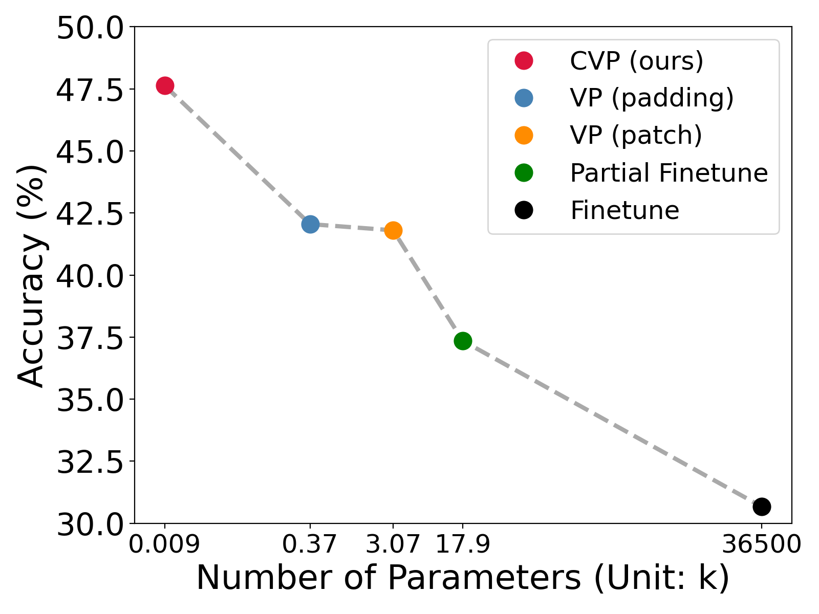
Figure 8:

7.5 More Evaluation

$\bullet$ We show more detailed results for CIFAR-10-C in Table 12 and  13.

	Standard	BN	Finetune	VP		CVP
				patch	append	fixed (3*3) w/o update	fixed (3*3) w/ update	rand (3*3) w/o update	rand (3*3) w/ update
Gaussian Noise	19.90	24.51	19.26	20.07	19.92	23.11	23.50	24.59	26.27
Shot Noise	20.37	24.25	19.43	20.56	20.40	22.95	23.32	24.29	25.26
Impulse Noise	27.44	26.14	19.19	27.54	27.44	30.76	30.98	31.13	31.08
Defocus Blur	12.90	14.54	13.39	13.59	13.18	16.81	17.41	18.85	20.03
Motion Blur	23.26	19.95	27.67	30.50	23.29	29.21	30.03	30.37	31.89
Glass Blur	25.97	33.30	18.61	19.70	26.01	36.14	37.54	37.42	40.51
Zoom Blur	71.08	50.46	42.42	71.07	71.06	86.76	87.65	85.76	88.19
Brightness	89.38	71.47	61.03	89.39	89.40	89.37	89.39	89.25	89.31
Snow	71.21	49.73	39.95	71.52	71.22	71.23	71.44	71.17	71.52
Frost	74.83	58.40	46.35	74.93	74.84	74.79	74.81	74.69	74.90
Fog	45.69	42.45	32.96	46.52	45.76	50.08	51.42	49.64	51.65
Contrast	58.36	49.87	39.22	57.95	58.47	67.74	68.99	69.05	70.21
Elastic Transform	17.54	24.01	19.95	17.72	17.56	17.39	17.62	18.07	19.66
Pixelate	23.45	39.80	34.26	24.10	23.50	25.91	26.47	28.39	30.58
Jpeg Compression	45.06	31.37	26.42	45.65	45.17	43.99	44.44	40.74	43.43
Avg. Acc.	41.76	37.35	30.67	42.05	41.82	45.75	46.33	46.23	47.63
Avg. Error	58.24	62.65	69.33	57.95	58.18	54.25	53.67	53.77	52.37
Avg Diff.	-	4.41	11.09	-0.29	-0.06	-3.99	-4.57	-4.46	-5.87

Table 12: Comparison of the different prompting methods with CVP for every CIFAR-10-C corruption type. The Standard model is WideResNet18. Number in bold shows the best performance.

Severity / Method	Standard	BN	Finetune	VP		CVP
				Patch	Append	fixed (3*3) w/o update	fixed (3*3) w/ update	rand. (3*3) w/o update	rand. (3*3) w/ update
S1	59.68	52.48	43.28	59.94	59.76	65.17	66.00	65.98	68.07
S2	47.88	43.18	34.72	48.26	47.94	52.73	53.42	53.41	54.73
S3	40.31	36.44	29.08	40.67	40.32	44.22	44.87	44.51	45.96
S4	32.75	29.49	24.66	32.94	32.75	36.20	36.74	36.56	37.79
S5	28.20	25.16	21.63	28.46	28.25	30.42	30.64	30.68	31.61
Avg. Acc.	41.76	37.35	30.67	42.05	41.82	45.75	46.33	46.23	47.63
Avg. Error	58.24	62.65	69.33	57.95	58.18	54.25	53.67	53.77	52.37
Avg Diff.	-	4.41	11.09	-0.29	-0.06	-3.99	-4.57	-4.46	-5.87

Table 13: Comparison of the different adaptation baslines with CVP for every severity on CIFAR-10-C. The Standard model is WideResNet18. Number in bold shows the best performance.

$\bullet$ More evaluation on ViT-Base model architecture. As Table 14 shows, we evaluate on 15 types of corruption under severity level 1 for CIFAR-10-C. The test accuracy of ViT-Base clean CIFAR-10 is 96.42%. Compared to the accuracy (%) before adaptation (standard) and using VP to do the adaptation, the CVP achieves better performance by up to 2 points.

	ViT-Base	VP	CVP
Gaussian Noise	47.64	49.71	50.22
Shot Noise	41.92	45.67	46.03
Impulse Noise	80.77	80.39	82.13
Glass Blur	48.49	47.77	49.12
Defocus Blur	27.91	27.37	28.90
Zoom Blur	83.71	83.23	85.63
Motion Blur	58.34	56.22	58.87
Brightness	94.40	93.10	94.59
Snow	89.37	88.23	89.41
Frost	90.13	92.19	92.32
Fog	74.75	73.60	75.63
Contrast	90.14	91.34	92.34
Pixelate	66.06	66.37	63.53
Jpeg Compression	62.53	61.55	63.53
Elastic Transform	40.68	40.52	41.52
Averaged Acc.	66.45	66.48	67.77

Table 14: Performance on ViT-Base model.

$\bullet$ We show the detailed results for each corruption on ImageNet-C dataset in Table 15.

$\bullet$ In Table 16, we further compare with TTT [59], which is a test-time method with CVP. We combine our CVP on top of TTT, where the model weight will first adapt based on the rotation loss, and then the input will adapt by convolutional visual prompt.

	Standard	Finetune	BN Adapt	VP		CVP
				patch	append	fixed 3*3	rand 3*3	fixed 5*5	rand 5*5
Gaussian Noise	80.00	78.85	79.43	79.44	79.99	78.49	78.16	78.47	78.75
Shot Noise	82.00	80.80	81.57	81.56	81.97	80.45	80.00	80.10	80.81
Impulse Noise	83.00	81.80	82.72	82.72	83.00	80.80	79.82	80.88	81.40
Defocus Blur	73.58	75.49	75.32	77.27	73.56	74.13	73.73	74.29	75.10
Motion Blur	90.95	79.85	92.38	80.18	77.96	89.99	89.31	89.14	88.60
Glass Blur	76.32	87.16	76.86	90.41	79.96	75.98	75.47	75.99	75.45
Zoom Blur	80.00	79.84	80.52	82.07	88.98	79.87	79.67	79.72	79.45
Snow	43.86	45.10	45.82	47.88	47.95	44.24	44.27	44.60	44.91
Frost	79.88	81.04	82.22	83.78	74.99	80.12	80.19	79.69	80.05
Fog	74.38	75.74	76.80	78.06	64.38	74.53	74.91	74.36	74.85
Brightness	78.25	79.90	81.23	84.99	88.07	78.78	78.49	78.83	78.91
Contrast	71.00	73.27	74.14	76.59	70.98	71.46	70.83	71.31	71.79
Elastic Transform	87.58	87.96	88.89	96.50	87.62	87.93	87.85	87.42	88.15
Pixelate	74.72	74.22	75.75	78.30	74.68	67.05	63.98	67.29	64.15
Jpeg Compression	77.00	75.47	74.85	81.29	76.99	74.41	73.46	74.05	74.26
mCE	76.83	77.10	77.90	80.07	76.74	75.88	75.34	75.74	75.77
Diff.		0.27	1.07	3.24	-0.09	-0.95	-1.49	-1.09	-1.06

Table 15: ImageNet-C results. Number in bold shows the lowest mCE.

	WideResNet18 Avg. Error (%)
Standard	58.24
VP (patch)	57.94 (-0.3)
CVP (rand. w/ update)	52.37 (-5.87)
TTT [63]	52.92 (-5.32)
TTT + CVP	53.07 (-5.17)

Table 16: TTT [59] result for CIFAR-10-C

$\bullet$ Generalize to Cutout-and-Paste samples To justify that our method can be generalized to non-structured OOD, we do more experiments on other types of OOD samples, such as the Cutout-and-Paste samples. Here, we launch the experiment on the Waterbirds dataset, which is constructed by cropping out birds from images with "water" backgrounds in the Caltech-UCSD Birds-200-2011 (CUB) dataset [61] and transferring them onto backgrounds from the Places dataset [72]. We follow the GitHub repo and choose the "Forest" as our new background to generate the samples. The training of SSL is based on the pre-trained ResNet34 backbone model for the original CUB dataset. The original CUB (200 classes) accuracy for the backbone ResNet34 is 75.34%. We compare our CVP with self-supervised VP and demonstrate that CVP is more effective on the Cutouted-CUB dataset. The following table shows our results. Our CVP improves the result upon Standard by 1.61 points and VP by 1.3 points.

Cutouted-CUB (200)	Before Adapt	VP (patch)	CVP
Accuracy (%)	62.03	62.32	63.64
contrastive loss (Avg.)	2.78	2.71	2.52

Table 17: Performance on the Cutouted-CUB

7.6 Distance measurement with SWD and SSIM

As the main paper mentioned, we measure the SWD and SSID on two input distributions: source domain distribution and target domain distribution (before/after adaptation). In Table 18 and Figure 9, we show the detailed result of SWD on every corruption type in CIFAR-10-C under severity 1. On average, CVP achieves lower SWD after adaptation, which means the target distribution is closer to the source one after adaptation. The average SWD reduced by 0.7% after prompting.

	SWD (scale: $10^{2}$) $\downarrow$		SSIM $\uparrow$
	before	after	before	after
Gaussian Noise	5.90	4.71	0.7242	0.7849
Shot Noise	6.08	4.93	0.7124	0.7676
Impulse Noise	6.23	5.26	0.7463	0.7764
Glass Blur	8.85	9.19	0.5873	0.5865
Defocus Blur	13.52	11.82	0.6031	0.6013
Zoom Blur	4.13	3.09	0.8726	0.8703
Motion Blur	7.68	5.57	0.6491	0.6459
Brightness	2.48	3.94	0.9702	0.9692
Snow	5.18	6.07	0.8258	0.8275
Frost	7.61	7.72	0.8025	0.8012
Fog	13.49	9.99	0.5840	0.5785
Contrast	15.39	11.09	0.7049	0.6997
Pixelate	3.09	4.56	0.8603	0.8669
Jpeg Compression	2.58	3.65	0.8681	0.8710
Elastic Transform	5.62	5.75	0.5272	0.5789
Avg. Mean	7.19	6.49	0.7539	0.7884
Avg. Std	4.05	2.79	0.1294	0.7260

Table 18: Results of Sliced Wasserstein Distance and Structural Similarity Index Measure on CIFAR-10-C (Severity 1).

(a) Noise Group

(b) Blur Group

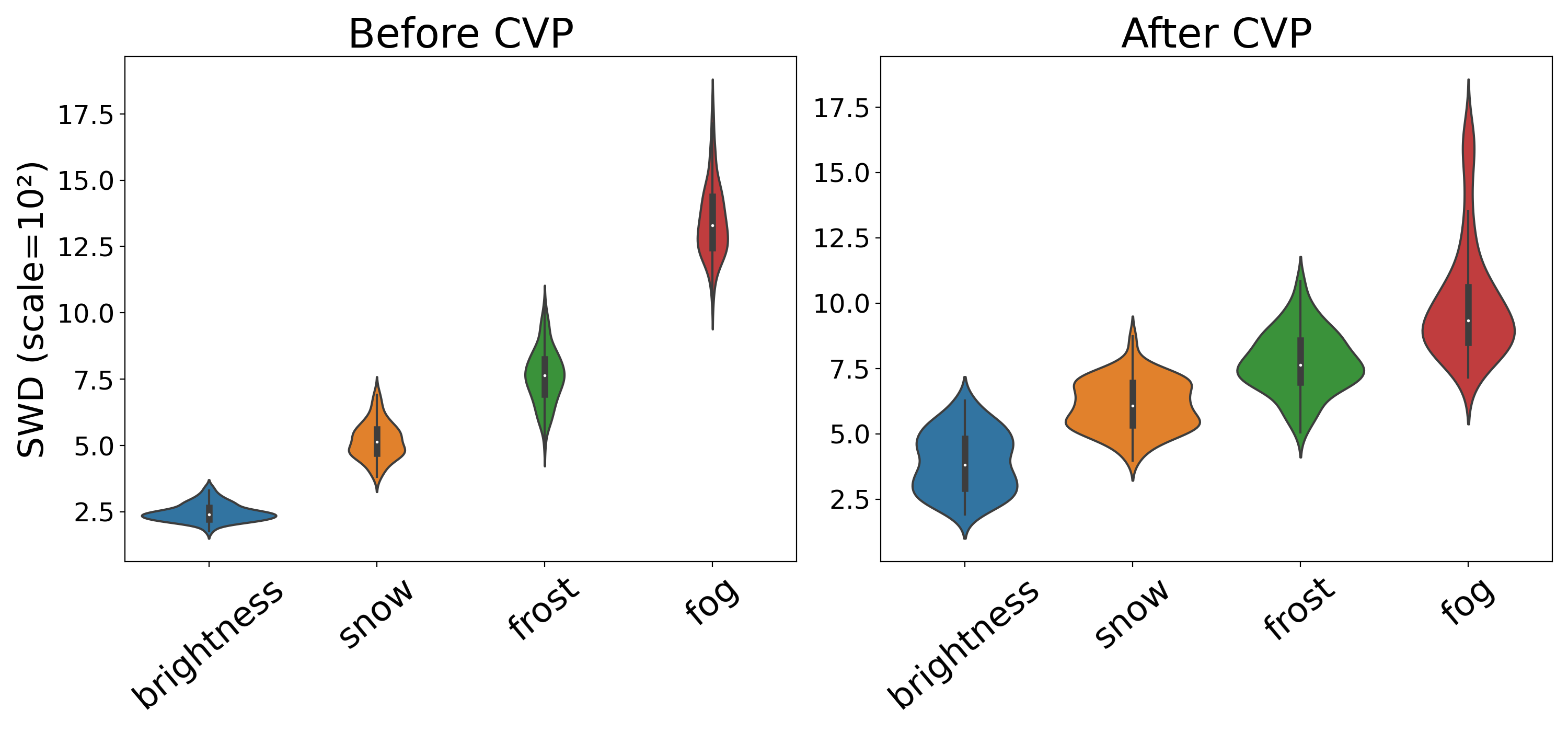
(c) Weather Group

(d) Digital Group

Figure 9: Violin Plot of SWD for different corruption groups on CIFAR-10-C. The left figure of each subplot shows the SWD before adapting, and the right shows the SWD after adaptation

$\bullet$ Distribution changes after applying the proposed CVP

In the main paper, Figure 2, we show the distribution changes in different corruption types and severity. Here, in Table 19, we show the distribution shifts after applying our CVP by calculating the average loss. In general, the distribution moves back to the original distribution. We show the SSL average loss (before adapt/after CVP adapt) for four corruption types on severity 1,3,5 for CIFAR10-C. The average SSL loss for the original CIFAR10 is 1.26. For every corruption we show here, the average SSL loss after adaptation is lower than the loss before adaptation.

severity	s1	s3	s5
	Before /After	Before /After	Before /After
Gaussian noise	1.9 / 1.6	2.5 / 2.1	3.3 / 2.6
Defocus blur	3.2 / 2.9	3.4 / 2.8	3.7 / 3.1
Snow	3.1 / 3.0	3.8 / 3.3	3.9 / 3.5
Contrast	2.7 / 2.3	2.9 / 2.4	3.6 / 3.3

Table 19: Distribution changes on different corruption types.

7.7 The Effect of Different Prompt Designs

We do analysis on different prompting methods, including original visual prompts with different norm-bound ($\ell_{2}$, $\ell_{\infty}$), convolutional prompts, and their combinations ($\ell_{2}+conv.$, $\ell_{\infty}+conv.$). We show the error rate on different numbers of adapt iters for every prompting method from 0, 1, 5, to 10. To compare the results, we set up other parameters such as the epsilon $\epsilon$ as $8/255$ for $\ell_{\infty}$, $1$ for $\ell_{2}$. As Figure 10 shows the error rate for different prompting methods, the convolutional prompt $conv.$ and its combination with $\ell_{2}$ reduce the error rate, and the former one reduces more from 40.32% to 36.08% when increasing the adapt iters. However, other prompting methods increase the error rate after prompting. To understand the risk of over-fitting for different prompting methods, Figure 4(b) shows the SSL loss curve v.s. performance on different prompting methods.

Figure 10:

7.8 Analysis on CVP and low-rank prompts

In Table 20, we show the detailed results of low-rank prompt (LVP) on different severity (from 1 to 5) for CIFAR-10-C. We set up the same rank as 3 for LVP and CVP. Our results show that the CVP is more effective than LVP when reversing natural corruption. In Figure 11, we further plot the averaged contrastive loss on different rank sizes for both LVP and CVP. On every corruption type, while increasing the rank size from 3 to 31, the loss curves of LVP consistently drop, which demonstrates the LVP is much more easier to overfit the contrastive loss.

Severity / Method	Standard	LVP	CVP
s1	40.32	37.05	31.93
s2	52.12	48.83	45.27
s3	59.69	56.05	54.04
s4	67.25	63.42	62.21
s5	71.80	68.89	68.39
Avg. Error	58.24	54.85	52.37
Diff.		-3.39	-5.87

Table 20:

(a)

(b)

Figure 11: In subfigure a., We show the $\ell_{2}$ distance between the ground-truth additive corruptions vector $\Delta$ and our prompt reversing vectors $\delta$. Subfigure b shows the averaged contrastive loss of low-rank prompt and CVP on different rank sizes. For every corruption type, the loss curves of LVP consistently drop when increasing the rank to 31 while the $\ell_{2}$ distances increase, demonstrating how LVP is more prone to overfitting the contrastive loss.

7.9 t-SNE analysis on different adaptation methods.

In addition to performing analysis on single sample, we further conduct the t-SNE visualization for whole sample distribution on different baseline. For each type of corruption data, we extract the 1-dimensional logit features in the last layer of model and calculate the distance between them with respect to the predicted class labels. We compare our method with standard, MEMO, and MEMO + Ours. As Figure 12 shows, the original feature embedding shows low separability between different classes. On the other hand, our approach clearly discriminates the embedding feature, which demonstrates its robustness against distribution shifts.

(a) Motion Blur

(b) Impulse Noise

Figure 12:

7.10 Saliency map analysis on different corruption types

To better understand how self-supervised visual prompts adapt to the corrupted inputs, we visualize the saliency map of different types of corruption. As Figure 13 shows, from left to right, the first row is the original, corrupted, and adapted samples; the second row shows their corresponding Grad-CAM with respect to the predicted labels. The red region in Grad-CAM shows where the model focuses on for target input. We empirically discover the heap map defocus on the target object for corrupted samples. However, after prompting, the red region of the adapted sample’s heap map is re-target on the similar region as original image, which demonstrates that the self-supervised visual prompts indeed improve the input adaptation and make the model refocus back on the correct regions.

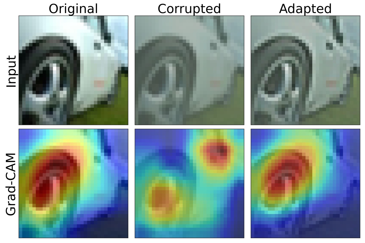
(a) Contrast

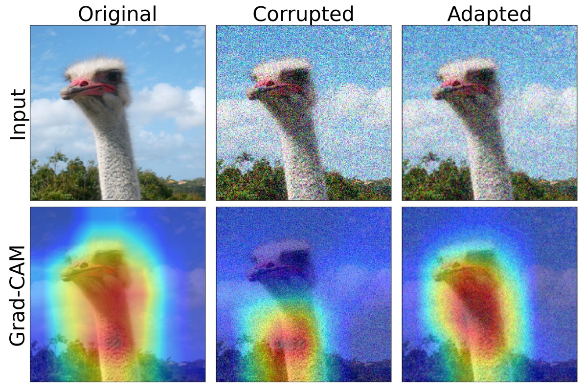
(b) Gaussian Noise

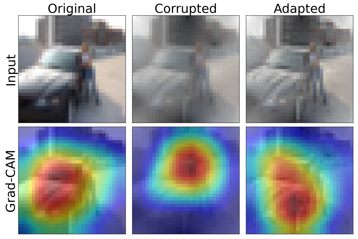
(c) Fog

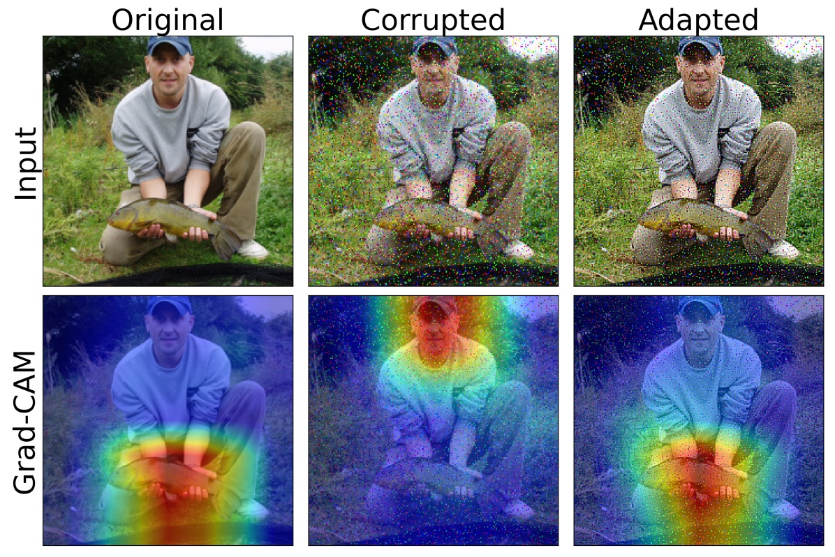
(d) Impulse noise

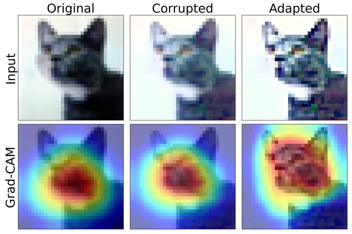
(e) Brightness

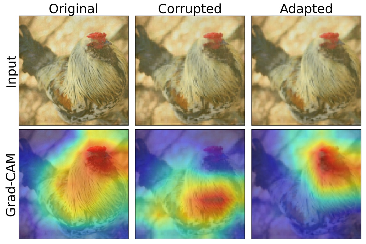
(f) Pixelate

Figure 13: Grad-CAM analysis on different types of corruption.

References

- [1] Hyojin Bahng, Ali Jahanian, Swami Sankaranarayanan, and Phillip Isola. Visual prompting: Modifying pixel space to adapt pre-trained models. arXiv preprint arXiv:2203.17274, 2022.
- [2] Tom Brown, Benjamin Mann, Nick Ryder, Melanie Subbiah, Jared D Kaplan, Prafulla Dhariwal, Arvind Neelakantan, Pranav Shyam, Girish Sastry, Amanda Askell, et al. Language models are few-shot learners. Advances in neural information processing systems, 33:1877–1901, 2020.
- [3] Mathilde Caron, Ishan Misra, Julien Mairal, Priya Goyal, Piotr Bojanowski, and Armand Joulin. Unsupervised learning of visual features by contrasting cluster assignments. In H. Larochelle, M. Ranzato, R. Hadsell, M.F. Balcan, and H. Lin, editors, Advances in Neural Information Processing Systems, volume 33, pages 9912–9924. Curran Associates, Inc., 2020.
- [4] Ting Chen, Simon Kornblith, Mohammad Norouzi, and Geoffrey Hinton. A simple framework for contrastive learning of visual representations. In International conference on machine learning, pages 1597–1607. PMLR, 2020.
- [5] Ting Chen, Simon Kornblith, Kevin Swersky, Mohammad Norouzi, and Geoffrey Hinton. Big self-supervised models are strong semi-supervised learners. arXiv preprint arXiv:2006.10029, 2020.
- [6] Xinlei Chen, Haoqi Fan, Ross Girshick, and Kaiming He. Improved baselines with momentum contrastive learning. arXiv preprint arXiv:2003.04297, 2020.
- [7] Virginia R de Sa. Learning classification with unlabeled data. Advances in neural information processing systems, pages 112–112, 1994.
- [8] Carl Doersch, Abhinav Gupta, and Alexei A Efros. Unsupervised visual representation learning by context prediction. In Proceedings of the IEEE international conference on computer vision, pages 1422–1430, 2015.
- [9] Alexey Dosovitskiy, Lucas Beyer, Alexander Kolesnikov, Dirk Weissenborn, Xiaohua Zhai, Thomas Unterthiner, Mostafa Dehghani, Matthias Minderer, Georg Heigold, Sylvain Gelly, et al. An image is worth 16x16 words: Transformers for image recognition at scale. arXiv preprint arXiv:2010.11929, 2020.
- [10] Qi Dou, Daniel Coelho de Castro, Konstantinos Kamnitsas, and Ben Glocker. Domain generalization via model-agnostic learning of semantic features. Advances in Neural Information Processing Systems, 32, 2019.
- [11] Gamaleldin F Elsayed, Ian Goodfellow, and Jascha Sohl-Dickstein. Adversarial reprogramming of neural networks. arXiv preprint arXiv:1806.11146, 2018.
- [12] Yaroslav Ganin and Victor Lempitsky. Unsupervised domain adaptation by backpropagation. In International conference on machine learning, pages 1180–1189. PMLR, 2015.
- [13] Robert Geirhos, Jörn-Henrik Jacobsen, Claudio Michaelis, Richard Zemel, Wieland Brendel, Matthias Bethge, and Felix A Wichmann. Shortcut learning in deep neural networks. Nature Machine Intelligence, 2(11):665–673, 2020.
- [14] Spyros Gidaris, Praveer Singh, and Nikos Komodakis. Unsupervised representation learning by predicting image rotations. arXiv preprint arXiv:1803.07728, 2018.
- [15] Kaiming He, Xinlei Chen, Saining Xie, Yanghao Li, Piotr Dollár, and Ross Girshick. Masked autoencoders are scalable vision learners. arXiv:2111.06377, 2021.
- [16] Kaiming He, Haoqi Fan, Yuxin Wu, Saining Xie, and Ross Girshick. Momentum contrast for unsupervised visual representation learning. In Proceedings of the IEEE/CVF conference on computer vision and pattern recognition, pages 9729–9738, 2020.
- [17] Kaiming He, Xiangyu Zhang, Shaoqing Ren, and Jian Sun. Deep residual learning for image recognition. In Proceedings of the IEEE conference on computer vision and pattern recognition, pages 770–778, 2016.
- [18] Dan Hendrycks, Steven Basart, Norman Mu, Saurav Kadavath, Frank Wang, Evan Dorundo, Rahul Desai, Tyler Zhu, Samyak Parajuli, Mike Guo, et al. The many faces of robustness: A critical analysis of out-of-distribution generalization. In Proceedings of the IEEE/CVF International Conference on Computer Vision, pages 8340–8349, 2021.
- [19] Dan Hendrycks, Steven Basart, Norman Mu, Saurav Kadavath, Frank Wang, Evan Dorundo, Rahul Desai, Tyler Zhu, Samyak Parajuli, Mike Guo, Dawn Song, Jacob Steinhardt, and Justin Gilmer. The many faces of robustness: A critical analysis of out-of-distribution generalization. 2021 IEEE/CVF International Conference on Computer Vision (ICCV), Oct 2021.
- [20] Dan Hendrycks and Thomas Dietterich. Benchmarking neural network robustness to common corruptions and perturbations. arXiv preprint arXiv:1903.12261, 2019.
- [21] Dan Hendrycks and Thomas Dietterich. Benchmarking neural network robustness to common corruptions and perturbations. Proceedings of the International Conference on Learning Representations, 2019.
- [22] Dan Hendrycks, Mantas Mazeika, Saurav Kadavath, and Dawn Song. Using self-supervised learning can improve model robustness and uncertainty. Advances in Neural Information Processing Systems, 32, 2019.
- [23] Dan Hendrycks, Kevin Zhao, Steven Basart, Jacob Steinhardt, and Dawn Song. Natural adversarial examples. CVPR, 2021.
- [24] Edward J Hu, Yelong Shen, Phillip Wallis, Zeyuan Allen-Zhu, Yuanzhi Li, Shean Wang, Lu Wang, and Weizhu Chen. Lora: Low-rank adaptation of large language models. arXiv preprint arXiv:2106.09685, 2021.
- [25] Xu Ji, Joao F Henriques, and Andrea Vedaldi. Invariant information clustering for unsupervised image classification and segmentation. In Proceedings of the IEEE/CVF International Conference on Computer Vision, pages 9865–9874, 2019.
- [26] Menglin Jia, Luming Tang, Bor-Chun Chen, Claire Cardie, Serge Belongie, Bharath Hariharan, and Ser-Nam Lim. Visual prompt tuning. arXiv preprint arXiv:2203.12119, 2022.
- [27] Eliska Kloberdanz, Jin Tian, and Wei Le. An improved (adversarial) reprogramming technique for neural networks. In Igor Farkavs, Paolo Masulli, Sebastian Otte, and Stefan Wermter, editors, Artificial Neural Networks and Machine Learning – ICANN 2021, pages 3–15, Cham, 2021. Springer International Publishing.
- [28] Alex Krizhevsky, Ilya Sutskever, and Geoffrey E Hinton. Imagenet classification with deep convolutional neural networks. Communications of the ACM, 60(6):84–90, 2017.
- [29] Gustav Larsson, Michael Maire, and Gregory Shakhnarovich. Learning representations for automatic colorization. In European conference on computer vision, pages 577–593. Springer, 2016.
- [30] Yann LeCun, Koray Kavukcuoglu, and Clément Farabet. Convolutional networks and applications in vision. In Proceedings of 2010 IEEE international symposium on circuits and systems, pages 253–256. IEEE, 2010.
- [31] Bo Li, Yezhen Wang, Shanghang Zhang, Dongsheng Li, Kurt Keutzer, Trevor Darrell, and Han Zhao. Learning invariant representations and risks for semi-supervised domain adaptation. In Proceedings of the IEEE/CVF Conference on Computer Vision and Pattern Recognition, pages 1104–1113, 2021.
- [32] Da Li, Yongxin Yang, Yi-Zhe Song, and Timothy M Hospedales. Learning to generalize: Meta-learning for domain generalization. In Thirty-Second AAAI Conference on Artificial Intelligence, 2018.
- [33] Yanghao Li, Naiyan Wang, Jianping Shi, Jiaying Liu, and Xiaodi Hou. Revisiting batch normalization for practical domain adaptation, 2016.
- [34] Zhiyuan Li, Yi Zhang, and Sanjeev Arora. Why are convolutional nets more sample-efficient than fully-connected nets? arXiv preprint arXiv:2010.08515, 2020.
- [35] Ziwei Liu, Zhongqi Miao, Xingang Pan, Xiaohang Zhan, Dahua Lin, Stella X Yu, and Boqing Gong. Open compound domain adaptation. In Proceedings of the IEEE/CVF Conference on Computer Vision and Pattern Recognition, pages 12406–12415, 2020.
- [36] Mingsheng Long, Yue Cao, Jianmin Wang, and Michael Jordan. Learning transferable features with deep adaptation networks. In International conference on machine learning, pages 97–105. PMLR, 2015.
- [37] Ilya Loshchilov and Frank Hutter. SGDR: Stochastic gradient descent with warm restarts. In International Conference on Learning Representations, 2017.
- [38] Zhihe Lu, Yongxin Yang, Xiatian Zhu, Cong Liu, Yi-Zhe Song, and Tao Xiang. Stochastic classifiers for unsupervised domain adaptation. In Proceedings of the IEEE/CVF Conference on Computer Vision and Pattern Recognition, pages 9111–9120, 2020.
- [39] Chengzhi Mao, Augustine Cha, Amogh Gupta, Hao Wang, Junfeng Yang, and Carl Vondrick. Generative interventions for causal learning. In Proceedings of the IEEE/CVF Conference on Computer Vision and Pattern Recognition, pages 3947–3956, 2021.
- [40] Chengzhi Mao, Mia Chiquier, Hao Wang, Junfeng Yang, and Carl Vondrick. Adversarial attacks are reversible with natural supervision. arXiv preprint arXiv:2103.14222, 2021.
- [41] Chengzhi Mao, Scott Geng, Junfeng Yang, Xin Wang, and Carl Vondrick. Understanding zero-shot adversarial robustness for large-scale models. arXiv preprint arXiv:2212.07016, 2022.
- [42] Chengzhi Mao, Lu Jiang, Mostafa Dehghani, Carl Vondrick, Rahul Sukthankar, and Irfan Essa. Discrete representations strengthen vision transformer robustness. arXiv preprint arXiv:2111.10493, 2021.
- [43] Chengzhi Mao, Revant Teotia, Amrutha Sundar, Sachit Menon, Junfeng Yang, Xin Wang, and Carl Vondrick. Doubly right object recognition: A why prompt for visual rationales. In Proceedings of the IEEE/CVF Conference on Computer Vision and Pattern Recognition (CVPR), pages 2722–2732, June 2023.
- [44] Chengzhi Mao, Kevin Xia, James Wang, Hao Wang, Junfeng Yang, Elias Bareinboim, and Carl Vondrick. Causal transportability for visual recognition. In Proceedings of the IEEE/CVF Conference on Computer Vision and Pattern Recognition, pages 7521–7531, 2022.
- [45] Chengzhi Mao, Lingyu Zhang, Abhishek Joshi, Junfeng Yang, Hao Wang, and Carl Vondrick. Robust perception through equivariance. arXiv preprint arXiv:2212.06079, 2022.
- [46] Claudio Michaelis, Benjamin Mitzkus, Robert Geirhos, Evgenia Rusak, Oliver Bringmann, Alexander S. Ecker, Matthias Bethge, and Wieland Brendel. Benchmarking robustness in object detection: Autonomous driving when winter is coming. arXiv preprint arXiv:1907.07484, 2019.
- [47] Mehdi Noroozi and Paolo Favaro. Unsupervised learning of visual representations by solving jigsaw puzzles. In European conference on computer vision, pages 69–84. Springer, 2016.
- [48] Taesung Park, Alexei A Efros, Richard Zhang, and Jun-Yan Zhu. Contrastive learning for unpaired image-to-image translation. In European Conference on Computer Vision, pages 319–345. Springer, 2020.
- [49] Kexin Pei, Yinzhi Cao, Junfeng Yang, and Suman Jana. Deepxplore: Automated whitebox testing of deep learning systems. In proceedings of the 26th Symposium on Operating Systems Principles, pages 1–18, 2017.
- [50] Juan C Pérez, Motasem Alfarra, Guillaume Jeanneret, Laura Rueda, Ali Thabet, Bernard Ghanem, and Pablo Arbeláez. Enhancing adversarial robustness via test-time transformation ensembling. In Proceedings of the IEEE/CVF International Conference on Computer Vision, pages 81–91, 2021.
- [51] Alec Radford, Jong Wook Kim, Chris Hallacy, Aditya Ramesh, Gabriel Goh, Sandhini Agarwal, Girish Sastry, Amanda Askell, Pamela Mishkin, Jack Clark, et al. Learning transferable visual models from natural language supervision. In International Conference on Machine Learning, pages 8748–8763. PMLR, 2021.
- [52] Alec Radford, Karthik Narasimhan, Tim Salimans, Ilya Sutskever, et al. Improving language understanding by generative pre-training. 2018.
- [53] Benjamin Recht, Rebecca Roelofs, Ludwig Schmidt, and Vaishaal Shankar. Do imagenet classifiers generalize to imagenet? In International Conference on Machine Learning, pages 5389–5400. PMLR, 2019.
- [54] Kate Saenko, Brian Kulis, Mario Fritz, and Trevor Darrell. Adapting visual category models to new domains. In European conference on computer vision, pages 213–226. Springer, 2010.
- [55] Shiori Sagawa, Pang Wei Koh, Tatsunori B. Hashimoto, and Percy Liang. Distributionally robust neural networks for group shifts: On the importance of regularization for worst-case generalization, 2019.
- [56] Kuniaki Saito, Kohei Watanabe, Yoshitaka Ushiku, and Tatsuya Harada. Maximum classifier discrepancy for unsupervised domain adaptation. In Proceedings of the IEEE conference on computer vision and pattern recognition, pages 3723–3732, 2018.
- [57] Vikash Sehwag, Mung Chiang, and Prateek Mittal. Ssd: A unified framework for self-supervised outlier detection. arXiv preprint arXiv:2103.12051, 2021.
- [58] Yu Sun, Xiaolong Wang, Zhuang Liu, John Miller, Alexei Efros, and Moritz Hardt. Test-time training with self-supervision for generalization under distribution shifts. In Hal Daumé III and Aarti Singh, editors, Proceedings of the 37th International Conference on Machine Learning, volume 119 of Proceedings of Machine Learning Research, pages 9229–9248. PMLR, 13–18 Jul 2020.
- [59] Yu Sun, Xiaolong Wang, Zhuang Liu, John Miller, Alexei A. Efros, and Moritz Hardt. Test-time training with self-supervision for generalization under distribution shifts, 2019.
- [60] Yun-Yun Tsai, Pin-Yu Chen, and Tsung-Yi Ho. Transfer learning without knowing: Reprogramming black-box machine learning models with scarce data and limited resources. In International Conference on Machine Learning, pages 9614–9624. PMLR, 2020.
- [61] Catherine Wah, Steve Branson, Peter Welinder, Pietro Perona, and Serge Belongie. The caltech-ucsd birds-200-2011 dataset. 2011.
- [62] Dequan Wang, Evan Shelhamer, Shaoteng Liu, Bruno Olshausen, and Trevor Darrell. Tent: Fully test-time adaptation by entropy minimization, 2020.
- [63] Dequan Wang, Evan Shelhamer, Shaoteng Liu, Bruno Olshausen, and Trevor Darrell. Tent: Fully test-time adaptation by entropy minimization. In International Conference on Learning Representations, 2021.
- [64] Haohan Wang, Songwei Ge, Zachary Lipton, and Eric P Xing. Learning robust global representations by penalizing local predictive power. In H. Wallach, H. Larochelle, A. Beygelzimer, F. d'Alché-Buc, E. Fox, and R. Garnett, editors, Advances in Neural Information Processing Systems, volume 32. Curran Associates, Inc., 2019.
- [65] Haohan Wang, Songwei Ge, Zachary Lipton, and Eric P Xing. Learning robust global representations by penalizing local predictive power. In Advances in Neural Information Processing Systems, pages 10506–10518, 2019.
- [66] Chao-Han Huck Yang, Yun-Yun Tsai, and Pin-Yu Chen. Voice2series: Reprogramming acoustic models for time series classification, 2021.
- [67] Yuzhe Yang, Guo Zhang, Dina Katabi, and Zhi Xu. Me-net: Towards effective adversarial robustness with matrix estimation. arXiv preprint arXiv:1905.11971, 2019.
- [68] Yuan Yao, Ao Zhang, Zhengyan Zhang, Zhiyuan Liu, Tat-Seng Chua, and Maosong Sun. Cpt: Colorful prompt tuning for pre-trained vision-language models. arXiv preprint arXiv:2109.11797, 2021.
- [69] Sergey Zagoruyko and Nikos Komodakis. Wide residual networks. arXiv preprint arXiv:1605.07146, 2016.
- [70] Zhiyuan Zeng, Keqing He, Yuanmeng Yan, Hong Xu, and Weiran Xu. Adversarial self-supervised learning for out-of-domain detection. In Proceedings of the 2021 Conference of the North American Chapter of the Association for Computational Linguistics: Human Language Technologies, pages 5631–5639, 2021.
- [71] M. Zhang, S. Levine, and C. Finn. MEMO: Test time robustness via adaptation and augmentation. 2021.
- [72] Bolei Zhou, Àgata Lapedriza, Aditya Khosla, Aude Oliva, and Antonio Torralba. Places: A 10 million image database for scene recognition. IEEE Transactions on Pattern Analysis and Machine Intelligence, PP:1–1, 07 2017.
- [73] Kaiyang Zhou, Yongxin Yang, Timothy Hospedales, and Tao Xiang. Deep domain-adversarial image generation for domain generalisation. In Proceedings of the AAAI Conference on Artificial Intelligence, volume 34, pages 13025–13032, 2020.
- [74] Kaiyang Zhou, Yongxin Yang, Yu Qiao, and Tao Xiang. Domain generalization with mixstyle. arXiv preprint arXiv:2104.02008, 2021.