On the Capacity Region of Optical Intensity Broadcast Channels

Abstract

This paper investigates the capacity region of the optical intensity broadcast channels (OI-BCs), where the input is subject to a peak-intensity constraint, an average-intensity constraint, or both. By leveraging the decomposition results of several random variables, i.e., uniform, exponential, and truncated exponential random variables, and adopting a superposition coding (SC) scheme, the inner bound on the capacity region is derived. Then, the outer bound is derived by applying the conditional entropy power inequality (EPI). In the high signal-to-noise ratio (SNR) regime, the inner bound asymptotically matches the outer bound, thus characterizing the high-SNR asymptotic capacity region. The bounds are also extended to the general $K$-user BCs without loss of high-SNR asymptotic optimality.

I Introduction

Recent years have witnessed rapid development and improvement of wireless communication technology, which has brought the vast popularity of the application of smartphones, intelligent robots, and driverless cars [1, 2, 3]. These mobile terminals provide great convenience to our daily lives. With the increasing number of mobile terminals and the demand for stable and high-speed data transmission, the traditional radio frequency (RF) wireless spectrum is facing severe congestion. To cope with this problem, we urgently need an emerging wireless communication to compensate for the shortcomings of traditional RF communication.

Optical wireless communication (OWC), with the advantages of low cost and abundant bandwidth, has attracted extensive attention [4, 5, 6, 7]. In an OWC system, information is carried on the intensity of optical light emitted by light-emitting diodes (LEDs) or laser diodes (LDs) and detected by photodetectors, which is known as the intensity-modulation and direct-detection (IM-DD) scheme [8, 9]. This unique scheme leads to fundamental differences between the OWC and RF systems. Here, the input corresponds to the optical intensity signal. Hence it is real-valued and non-negative. Furthermore, the peak or/and average intensity are often constrained for the input with battery limitation and safety considerations [10, 11, 12, 13]. With the advancement of coding, modulation, and detection technologies, the OWC systems have been successfully applied in offices, hospitals, and airport cabins [14, 15, 16].

Generally, the OWC systems can be classified as outdoor free-space optical communication (FSO) and indoor visible light communication (VLC) systems [17, 18, 19]. In this paper, we mainly focus on the indoor VLC systems and explore them from an information-theoretic perspective. Extensive studies have been done on the channel capacity for single-user indoor VLC systems [10, 11, 20, 21, 22, 23, 24]. For example, the authors in [10] derived the upper and lower bounds on the single-user channel capacity when the input satisfies peak or/and average-intensity constraints. Besides, the asymptotic capacity results at low and high signal-to-noise ratios (SNRs) were also proposed. In recent years, there has been an increasing interest in the multi-user VLC networks, where the transmitter serves multiple users so that each user reliably receives messages simultaneously [25].

Considering the input satisfies peak- or/and average-intensity constraints, several studies have been done on the capacity region of the VLC networks, such as broadcast channels (BCs), multiple access channels (MACs), and interference channels (ICs) [26, 27, 28, 29]. For the BC network, the authors in [26] considered both peak- and average-intensity constraints for the input. They derived the inner bound on the capacity region based on the truncated Gaussian or on-off keying (OOK) coding scheme and the outer bound based on Bergmans’ approach. These bounds asymptotically matched at low SNR and achieved a constant gap at high SNR. For the MAC network, the authors in [27] adopted a similar method as in [26] and the derived bounds achieved similar performances. Different from [27], the authors in [28] considered the peak- or average-intensity constraint for the input. They derived the inner bound based on the uniform or exponential coding scheme, which achieved asymptotic optimality at high SNR. For the IC network, the authors in [29] considered both peak- and average-intensity constraints for the input. They derived the inner bound based on the treating-interference-as-noise (TIN) or Han-Kobayashi (HK) schemes and the outer bounds by providing different side information to the receivers.

In this paper, we investigate the optical intensity BCs (OI-BCs). Different from [26], here we consider the input is subject to three different intensity constraints: (1) only peak-intensity constraint; (2) only average-intensity constraint; (3) both peak- and average-intensity constraints. We provide new inner and outer bounds on the capacity region of the considered OI-BCs. Instead of the truncated Gaussian codes [26], we adopt a superposition coding (SC) scheme from the decomposition results of several random variables to derive the inner bound. These random variables are the maximal entropy-achieving inputs when considering peak- or/and average-intensity constraints [10]. The outer bound is derived by applying the conditional entropy power inequality (EPI) [30]. We show that the bounds are asymptotically optimal in the high-SNR regime. Moreover, we extend the bounds to the $K$-user OI-BCs without loss of high-SNR asymptotic optimality.

The remaining part of this paper is organized as follows. Sec. II introduces the channel model of the OI-BCs. Secs. III and IV analyze the capacity regions of two-user and $K$-user OI-BCs, respectively. We conclude this paper in Sec. V. A few proofs are given in the Appendices.

Notation: A random variable is denoted by an uppercase letter, e.g., $X$, while its realization by a smallcase letter, e.g., $x$. The support of a random variable is denoted by $\mathsf{supp}(\cdot)$, the expectation by $\mathbb{E}[\cdot]$, and the characteristic function by $\phi(\cdot)$. Differential entropy is denoted by $\mathsf{h}(\cdot)$ and mutual information by $\mathsf{I}(\cdot;\cdot)$. The set of non-negative real numbers is denoted by $\mathbb{R}^{+}$ and the set of positive natural numbers by $\mathbb{N}^{+}$. Dirac delta function is denoted by $\delta(\cdot)$ and the convex hull of a set by $\mathsf{Conv}\{\cdot\}$. The index set $\{1,2,\ldots,k\}$ is denoted by $[k]$, $k\in\mathbb{N}^{+}$, and $j=\sqrt{-1}$. Function $A(t)\doteq B(t)$ denotes that $\lim_{t\rightarrow\infty}\{A(t)-B(t)\}=0$.

II Channel Model

For a single-user optical intensity channel, the channel output is given by

$$Y=X+Z,$$ (1)

where $X$ denotes channel input and $Z$ denotes Gaussian noise with variance $\sigma^{2}$, i.e.,

$$Z\sim\mathcal{N}(0,\sigma^{2}).$$ (2)

Since $X$ is proportional to optical intensity, its support must satisfy

$$\mathsf{supp}(X)\subset\mathbb{R}^{+}.$$ (3)

Considering the limited dynamic range of LED devices and the requirement of illumination quality or energy consumption, the input is usually subject to a peak-intensity constraint:

$$\textnormal{Pr}(X\leq\textnormal{A})=1,$$ (4)

or/and an average-intensity constraint:

$$\mathbb{E}[X]\leq\textnormal{E}.$$ (5)

For convenience, we denote the ratio between the maximal instantaneous intensity and average intensity as $\alpha$, i.e., $\alpha=\frac{\textnormal{E}}{\textnormal{A}}$, which is limited in $\left(0,\frac{1}{2}\right]$.

In this paper, we mainly focus on the OI-BCs. We first consider a two-user OI-BC, and the channel output at user $k$ is given by

$$Y_{k}=X+Z_{k},\quad k\in\{1,2\},$$ (6)

where $X$ denotes the channel input, whose support satisfies (3), and is also subject to (4), or/and (5); and $Z_{k}$ denotes the Gaussian noise at user $k$, and

$$Z_{k}\sim\mathcal{N}(0,\sigma_{k}^{2}),\quad k\in\{1,2\}.$$ (7)

Without loss of generality, we assume $\sigma_{1}\leq\sigma_{2}$. Besides, a high SNR regime corresponds to the regime where $\textnormal{A}\gg\sigma_{k}$ or $\textnormal{E}\gg\sigma_{k}$, $k\in\{1,2\}$.

In a two-user OI-BC, the desired messages for users 1 and 2 are denoted by $M_{1}$ and $M_{2}$, respectively. We assume $M_{1}$ and $M_{2}$ are independent. The transmitter encodes and sends them at coding rates $R_{1}$, and $R_{2}$, respectively, and simultaneously. If both users can decode their messages with vanishing error probabilities as the code length tends to infinity, we say that the rate pair $(R_{1},R_{2})$ is achievable. The capacity region of this channel is the closure of the set of all achievable rate pairs.

Note that the channel in (6) belongs to the class of the additive white Gaussian broadcast channels, which is a physically degraded channel [25]. As a consequence, we have

$$Y_{2}=Y_{1}+\widetilde{Z}_{2},$$ (8)

where $\widetilde{Z}_{2}\sim\mathcal{N}(0,\sigma_{2}^{2}-\sigma_{1}^{2})$. The capacity region of a two-user physically degraded channel is characterized by [31, Theorem 15.6.2] and summarized in the following lemma:

Lemma 1.

The capacity region of the two-user OI-BC in (6), where $X\rightarrow Y_{1}\rightarrow Y_{2}$ forms a Markov chain, is the set of rate pair $(R_{1},R_{2})$ satisfying

$$R_{1} \leq \mathsf{I}(X;Y_{1}|U),$$ (9)

$$R_{2} \leq \mathsf{I}(U;Y_{2}),$$ (10)

for some $p_{U,X}(u,x)$ subject to (3), (4), or/and (5).

Above notations and assumptions can be directly extended to the $K$-user OI-BC, i.e.,

$$Y_{k}=X+Z_{k},\quad k\in[K],$$ (11)

where $X$ is a codeword of independent messages $M_{1},M_{2}\cdots,M_{K}$, and satisfies (3), (4), or/and (5); and $Z_{k}\sim\mathcal{N}(0,\sigma_{k}^{2})$, $k\in[K]$. Without loss of generality, we also assume $\sigma_{1}\leq\sigma_{2}\leq\ldots\leq\sigma_{K}$. It should be noted that the above $K$-user OI-BC is also a physically degraded channel, and we have

$$Y_{k+1}=Y_{k}+\widetilde{Z}_{k+1},\quad k\in[K-1],$$ (12)

where $\widetilde{Z}_{k+1}\sim\mathcal{N}(0,\sigma_{k+1}^{2}-\sigma_{k}^{2})$. The capacity region of a $K$-user physically degraded channel is characterized by [25, Chapter 5.7], [32, Theorem 3] and summarized in the following lemma:

Lemma 2.

The capacity region of the $K$-user OI-BC in (11), where $X\rightarrow Y_{1}\rightarrow Y_{2}\rightarrow\ldots\rightarrow Y_{K}$ forms a Markov chain, is the set of rate tuple $(R_{1},R_{2},\ldots,R_{K})$ satisfying

$$R_{k} \leq \mathsf{I}(U_{k};Y_{k}|U_{k+1}),\quad k\in[K],$$ (13)

for some $p_{U_{K-1}|U_{K}}(u_{K-1}|u_{K})p_{U_{K-2}|U_{K-1}}(u_{K-2}|u_{K-1})\cdots p_{U_{1}|U_{2}}(u_{1}|u_{2})$ subject to (3), (4), or/and (5), where $U_{1}=X$, $U_{K+1}=\emptyset$, .

III Capacity Region Characterization of Two-User OI-BCs

In this section, we characterize the capacity region of two-user OI-BCs with three different input constraints. In each case of input constraints, we first present some preliminaries about the decomposition of the random variable and the existing single-user channel capacity, then derive the inner and outer bounds on the capacity region. Finally, the high-SNR capacity region is characterized based on these bounds.

III-A Peak-Intensity Constrained OI-BC

III-A1 Preliminary

Considering the peak-intensity constraint in (4), the decomposition of a uniform random variable and the existing single-user channel capacity is introduced in the following.

Lemma 3 ([33]).

Given any integer $N\in\mathbb{N}^{+}$, a uniform random variable $S$, i.e.,

$$p_{S}(s)=\frac{1}{\textnormal{A}},\quad s\in[0,\textnormal{A}],$$ (14)

can be decomposed as a sum of two independent random variables $S_{1}$ and $S_{2}$, i.e.,

$$p_{S_{1}}(s_{1}) = \frac{N}{\textnormal{A}},\quad s_{1}\in\left[0,\frac{\textnormal{A}}{N}\right],$$ (15)

$$p_{S_{2}}(s_{2}) = \frac{1}{N}\sum_{n=0}^{N-1}\delta\left(s_{2}-\frac{n}{N}\times\textnormal{A}\right).$$ (16)

For convenience, the distribution in (14) is denoted by $\textsf{U}[0,\textnormal{A}]$.

Lemma 4 ([20, 10]).

The channel capacity $\mathsf{C}(\textnormal{A},\sigma)$ of a peak-intensity constrained optical intensity channel, is upper bounded by

$$\mathsf{C}_{\textnormal{ub}}(\textnormal{A},\sigma)=\min\left\{\frac{1}{2}\log\left(1+\frac{\textnormal{A}^{2}}{4\sigma^{2}}\right),\,\log\left(1+\frac{\textnormal{A}}{\sqrt{2\pi e}\sigma}\right)\right\},$$ (17)

At high SNR,

$$\mathsf{C}_{\textnormal{ub}}(\textnormal{A},\sigma)\doteq\frac{1}{2}\log\left(1+\frac{\textnormal{A}^{2}}{2\pi e\sigma^{2}}\right).$$ (18)

III-A2 Bounds on Capacity Region

The inner bound on the capacity region is derived based on the SC scheme.

Theorem 1 (Inner Bound).

When the input is only subject to the peak-intensity constraint in (4), the rate pairs in the set $\mathsf{Conv}\{\cup_{N\in\mathbb{N}^{+}}\left(R_{1}^{\textnormal{in}}(N),R_{2}^{\textnormal{in}}(N)\right)\}$ are all achievable for a two-user OI-BC, where

$${\Hy@raisedlink{\hyper@anchorstart{\@IEEEtheHrefequation}}\Hy@raisedlink{\hyper@anchorend}}R_{1}^{\textnormal{in}}(N) = \frac{1}{2}\log\left(1+\frac{\textnormal{A}^{2}}{2\pi eN^{2}\sigma_{1}^{2}}\right),$$ (19a)

$$R_{2}^{\textnormal{in}}(N) = \frac{1}{2}\log\left(1+\frac{\textnormal{A}^{2}}{2\pi e\sigma_{2}^{2}}\right)-\mathsf{C}_{\textnormal{ub}}\left(\frac{\textnormal{A}}{N},\sigma_{2}\right).$$ (19b)

Proof.

We first encode the messages $M_{1}$ and $M_{2}$ independently into signals $X_{1}$ and $X_{2}$, where $X_{1}$ follows $\textsf{U}[0,\frac{\textnormal{A}}{N}]$ and $X_{2}$ follows

$$p_{X_{2}}(x_{2}) = \frac{1}{N}\sum_{n=0}^{N-1}\delta\left(x_{2}-\frac{n}{N}\times\textnormal{A}\right).$$ (20)

Then we adopt an SC scheme such that $X=X_{1}+X_{2}$. By applying Lemma 3, we obtain that $X$ follows $\textsf{U}[0,\textnormal{A}]$, which satisfies the peak-intensity constraint in (4). In Lemma 1, we instantiate $U$ into $U=X_{2}$. Therefore, we can compute the achievable rates $\mathsf{I}(X;Y_{1}|X_{2})$ and $\mathsf{I}(X_{2};Y_{2})$ to be as the inner bounds on $R_{1}$ and $R_{2}$, respectively. On the one hand,

$$\mathsf{I}(X;Y_{1}|X_{2}) = \mathsf{I}(X_{1};X_{1}+Z_{1})$$ (21)

$$= \mathsf{h}(X_{1}+Z_{1})-\mathsf{h}(Z_{1})$$ (22)

$$\geq \frac{1}{2}\log\left(1+\frac{e^{2\mathsf{h}(X_{1})}}{e^{2\mathsf{h}(Z_{1})}}\right)$$ (23)

$$= \frac{1}{2}\log\left(1+\frac{\textnormal{A}^{2}}{2\pi eN^{2}\sigma_{1}^{2}}\right).$$ (24)

where (23) holds by the EPI. On the other hand,

$$\mathsf{I}(X_{2};Y_{2}) = \mathsf{h}(Y_{2})-\mathsf{h}(Y_{2}|X_{2})$$ (25)

$$= \mathsf{h}(X+Z_{2})-\mathsf{h}(X_{1}+Z_{2})$$ (26)

$$\geq \frac{1}{2}\log\left(e^{2\mathsf{h}(X)}+e^{2\mathsf{h}(Z_{2})}\right)-\mathsf{h}(X_{1}+Z_{2})$$ (27)

$$\geq \frac{1}{2}\log\left(1+\frac{\textnormal{A}^{2}}{2\pi e\sigma_{2}^{2}}\right)-\mathsf{C}_{\textnormal{ub}}\left(\frac{\textnormal{A}}{N},\sigma_{2}\right).$$ (28)

where (27) holds by the EPI; and (28) holds since $X_{1}$ is limited in $[0,\frac{\textnormal{A}}{N}]$ and independent of the Gaussian noise $Z_{2}$, thus we can bound $\mathsf{h}(X_{1}+Z_{2})$ by $\mathsf{h}(X_{1}+Z_{2})\leq\mathsf{C}_{\textnormal{ub}}\left(\frac{\textnormal{A}}{N},\sigma_{2}\right)+\mathsf{h}(Z_{2})$.

Combining (24) and (28), the rate pairs $\left(R_{1}^{\textnormal{in}}(N),R_{2}^{\textnormal{in}}(N)\right)$ in (19a) are achievable. Moreover, by adopting a time sharing strategy between these achievable rate pairs, the rate pairs in the set $\mathsf{Conv}\{\cup_{N\in\mathbb{N}^{+}}\left(R_{1}^{\textnormal{in}}(N),R_{2}^{\textnormal{in}}(N)\right)\}$ are all achievable. Finally, the proof is completed. ∎

The outer bound on the capacity region is derived based on the conditional EPI.

Theorem 2 (Outer Bound).

When the input is only subject to the peak-intensity constraint in (4), the capacity region is outer bounded by $\cup_{\rho\in[0,1]}\left(R_{1}^{\textnormal{out}}(\rho),R_{2}^{\textnormal{out}}(\rho)\right)$ for a two-user OI-BC, where

$${\Hy@raisedlink{\hyper@anchorstart{\@IEEEtheHrefequation}}\Hy@raisedlink{\hyper@anchorend}}R_{1}^{\textnormal{out}}(\rho) = \frac{1}{2}\log\left\{1+\frac{\sigma_{2}^{2}}{\sigma_{1}^{2}}\left(e^{2\mathsf{C}_{\textnormal{ub}}\left(\rho\textnormal{A},\sigma_{2}\right)}-1\right)\right\},$$ (29a)

$$R_{2}^{\textnormal{out}}(\rho) = \mathsf{C}_{\textnormal{ub}}\left(\textnormal{A},\sigma_{2}\right)-\mathsf{C}_{\textnormal{ub}}\left(\rho\textnormal{A},\sigma_{2}\right).$$ (29b)

Proof.

We resort to Lemma 1 to derive an upper bound on the achievable rate $R_{2}$ of user 2 first and then the achievable rate $R_{1}$ of user 1. When $U\rightarrow X\rightarrow Y_{2}$ forms a Markov chain, it follows that

$$\mathsf{h}(Y_{2}|U)\geq\mathsf{h}(Y_{2}|X)=\mathsf{h}(Z_{2}).$$ (30)

Furthermore, we have

$$\mathsf{h}(Y_{2}|U) \leq \mathsf{h}(Y_{2})\leq\mathsf{C}_{\textnormal{ub}}(\textnormal{A},\sigma_{2})+\mathsf{h}(Z_{2}).$$ (31)

Note that $\mathsf{C}_{\textnormal{ub}}(\textnormal{A},\sigma_{2})$ is monotonically increasing with respect to A and approaches zero when A tends to $0$. Combined with (30) and (31), there exists $\rho\in[0,1]$ such that

$$\mathsf{h}(Y_{2}|U)=\mathsf{C}_{\textnormal{ub}}(\rho\textnormal{A},\sigma_{2})+\mathsf{h}(Z_{2}).$$ (32)

Applying Lemma 1, the achievable rate $R_{2}$ can be upper bounded by

$$R_{2} \leq \mathsf{I}(U;Y_{2})$$ (33)

$$= \mathsf{h}(Y_{2})-\mathsf{h}(Y_{2}|U)$$ (34)

$$\leq \mathsf{C}_{\textnormal{ub}}(\textnormal{A},\sigma_{2})-\mathsf{C}_{\textnormal{ub}}(\rho\textnormal{A},\sigma_{2}),$$ (35)

where (35) is obtained by substituting $\mathsf{h}(Y_{2})\leq\mathsf{C}_{\textnormal{ub}}(\textnormal{A},\sigma_{2})+\mathsf{h}(Z_{2})$ and (32) into (34). Moreover, the achievable rate $R_{1}$ can be upper bounded by

$$R_{1} \leq \mathsf{I}(X;Y_{1}|U)$$ (36)

$$= \mathsf{h}(Y_{1}|U)-\mathsf{h}(Z_{1})$$ (37)

$$\leq \frac{1}{2}\log\left(e^{2\mathsf{h}(Y_{2}|U)}-e^{2\mathsf{h}(\widetilde{Z}_{2}|U)}\right)-\mathsf{h}(Z_{1})$$ (38)

$$= \frac{1}{2}\log\left\{1+\frac{\sigma_{2}^{2}}{\sigma_{1}^{2}}\left(e^{2\mathsf{C}_{\textnormal{ub}}\left(\rho\textnormal{A},\sigma_{2}\right)}-1\right)\right\},$$ (39)

where (38) is obtained by noting that $Y_{2}=Y_{1}+\widetilde{Z}_{2}$ and we can utilize the conditional EPI to bound $\mathsf{h}(Y_{1}|U)$ such that $\mathsf{h}(Y_{1}|U)\leq\frac{1}{2}\log\left(e^{2\mathsf{h}(Y_{2}|U)}-e^{2\mathsf{h}(\widetilde{Z}_{2}|U)}\right)$; and (39) is obtained by substituting (32) into (38). Combining (35) and (39), we complete the proof. ∎

The high-SNR capacity region is derived based on the inner bound in Theorem 1 and the outer bound in Theorem 2. We summarize it as follows.

Theorem 3 (Asymptotic Capacity Region).

When the input is only subject to the peak-intensity constraint in (4), at high SNR, the capacity region of a two-user OI-BC asymptotically converges to the region where the rate pair $(R_{1},R_{2})$ satisfies

$${\Hy@raisedlink{\hyper@anchorstart{\@IEEEtheHrefequation}}\Hy@raisedlink{\hyper@anchorend}}R_{1} \ \dot{\leq}\ \frac{1}{2}\log\left(1+\frac{\rho^{2}\textnormal{A}^{2}}{2\pi e\sigma_{1}^{2}}\right),$$ (40a)

$$R_{2} \ \dot{\leq}\ \frac{1}{2}\log\left(1+\frac{\left(1-\rho^{2}\right)\textnormal{A}^{2}}{\rho^{2}\textnormal{A}^{2}+2\pi e\sigma_{2}^{2}}\right),$$ (40b)

with $\rho\in[0,1]$.

Proof.

At high SNR, the single-user capacity result of peak-intensity constrained optical intensity channel is given in Lemma 4. Substituting it into Theorem 2, we obtain that the capacity region at high SNR is outer bounded by $\cup_{\rho\in[0,1]}\left(R_{1}^{\textnormal{out}}(\rho),R_{2}^{\textnormal{out}}(\rho)\right)$, where

$${\Hy@raisedlink{\hyper@anchorstart{\@IEEEtheHrefequation}}\Hy@raisedlink{\hyper@anchorend}}R_{1}^{\textnormal{out}}(\rho) \doteq \frac{1}{2}\log\left(1+\frac{\rho^{2}\textnormal{A}^{2}}{2\pi e\sigma_{1}^{2}}\right),$$ (41a)

$$R_{2}^{\textnormal{out}}(\rho) \doteq \frac{1}{2}\log\left(1+\frac{\left(1-\rho^{2}\right)\textnormal{A}^{2}}{\rho^{2}\textnormal{A}^{2}+2\pi e\sigma_{2}^{2}}\right).$$ (41b)

For convenience, we write the boundary of the above outer bound as

$$R_{2}^{\textnormal{out}} \doteq \frac{1}{2}\log\left(1+\frac{\textnormal{A}^{2}}{2\pi e\sigma_{2}^{2}}\right)-\frac{1}{2}\log\left(1+\frac{\sigma_{1}^{2}}{\sigma_{2}^{2}}\left(e^{2R_{1}}-1\right)\right),\ R_{1}\in\left[0,\frac{1}{2}\log\left(1+\frac{\textnormal{A}^{2}}{2\pi e\sigma_{1}^{2}}\right)\right].\quad$$ (42)

Next, we proceed to show that the inner bound in Theorem 1 is tight with (41a) at high SNR. Substituting (18) into (19a), we obtain that the rate pairs in $\mathsf{Conv}\{\cup_{N\in\mathbb{N}^{+}}\left(R_{1}^{\textnormal{in}}(N),R_{2}^{\textnormal{in}}(N)\right)\}$ are all achievable, where

$$R_{1}^{\textnormal{in}}(N) \doteq \frac{1}{2}\log\left(1+\frac{\textnormal{A}^{2}}{2\pi eN^{2}\sigma_{1}^{2}}\right),$$ (43)

$$R_{2}^{\textnormal{in}}(N) \doteq \frac{1}{2}\log\left(\frac{\textnormal{A}^{2}+2\pi e\sigma_{2}^{2}}{\textnormal{A}^{2}+2\pi eN^{2}\sigma_{2}^{2}}\times N^{2}\right).$$ (44)

To analyze the inner bound characterized by the above achievable rate pairs, we fix an integer $N$ and derive the convex hull of two adjacent rate pairs $\left(R_{1}^{\textnormal{in}}(N),R_{2}^{\textnormal{in}}(N)\right)$ and $(R_{1}^{\textnormal{in}}(N+1),R_{2}^{\textnormal{in}}(N+1))$, which is a straight line segment:

$$R_{2}^{\textnormal{in}} \doteq \frac{\log\left(\frac{\textnormal{A}^{2}+2\pi eN^{2}\sigma_{2}^{2}}{\textnormal{A}^{2}+2\pi e(N+1)^{2}\sigma_{2}^{2}}\times\frac{(N+1)^{2}}{N^{2}}\right)}{\log\left(\frac{\textnormal{A}^{2}+2\pi e(N+1)^{2}\sigma_{1}^{2}}{\textnormal{A}^{2}+2\pi eN^{2}\sigma_{1}^{2}}\times\frac{N^{2}}{(N+1)^{2}}\right)}\left(R_{1}-\frac{1}{2}\log\left(\frac{\textnormal{A}^{2}}{2\pi eN^{2}\sigma_{1}^{2}}\right)\right)+\frac{1}{2}\log\left(\frac{\textnormal{A}^{2}+2\pi e\sigma_{2}^{2}}{\textnormal{A}^{2}+N^{2}2\pi e\sigma_{2}^{2}}\times N^{2}\right)$$ (45)

$$\doteq -R_{1}+\frac{1}{2}\log\left(\frac{\textnormal{A}^{2}}{2\pi e\sigma_{1}^{2}}\right),\ R_{1}\in[R_{1}^{\textnormal{in}}(N),R_{1}^{\textnormal{in}}(N+1)],\ \forall N\in\mathbb{N}^{+}.$$

We compute the gap between $R_{2}^{\textnormal{out}}-R_{2}^{\textnormal{in}}$ such that

$$R_{2}^{\textnormal{out}}-R_{2}^{\textnormal{in}} \doteq \log\left(\frac{\sigma_{1}^{2}}{\sigma_{2}^{2}}\right)-\frac{1}{2}\log\left(1+\frac{\sigma_{1}^{2}}{\sigma_{2}^{2}}\left(e^{2R_{1}}-1\right)\right)+R_{1}$$ (46)

$$\doteq \log\left(\frac{\sigma_{1}^{2}}{\sigma_{2}^{2}}\right)-\frac{1}{2}\log\left(1+\frac{\rho^{2}\textnormal{A}^{2}}{2\pi e\sigma_{2}^{2}}\right)+\frac{1}{2}\log\left(1+\frac{\rho^{2}\textnormal{A}^{2}}{2\pi e\sigma_{1}^{2}}\right)$$ (47)

$$\doteq 0,\quad R_{1}\in[R_{1}^{\textnormal{in}}(N),R_{1}^{\textnormal{in}}(N+1)],\ \forall N\in\mathbb{N}^{+}.$$ (48)

where (47) is obtained by substituting (41a) into (46). When we take all the possible integer $N$ in $\mathbb{N}^{+}$, it follows that

$$R_{2}^{\textnormal{out}}-R_{2}^{\textnormal{in}} \doteq 0,\quad\forall R_{1}\in\left[0,\frac{1}{2}\log\left(1+\frac{\textnormal{A}^{2}}{2\pi e\sigma_{1}^{2}}\right)\right],$$ (49)

which indicates that the outer bound in Theorem 2 and inner bound in Theorem 1 are tight at high SNR. Hence, we complete the proof. ∎

The derived bounds on the capacity region are shown in Fig. 1, where we assume $\sigma_{2}=2\sigma_{1}$ and $\mathrm{ASNR}_{k}=\frac{\textnormal{A}}{\sigma_{k}}$, $k\in\{1,2\}$. From the figure, it is straightforward to observe that the inner and outer bounds become tighter as SNR increases, which numerically validates the derivations.

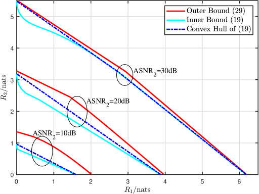
Figure 1: Bounds on capacity region of $2$-user OI-BC with peak-intensity constraint.

III-B Average-Intensity Constrained OI-BC

III-B1 Preliminary

Considering the average-intensity constraint in (5), the decomposition of an exponential random variable and the existing single-user channel capacity is introduced in the following.

Lemma 5 ([33]).

Given any $\textnormal{E}>0$, $\textnormal{E}_{1}>0$, and $\textnormal{E}_{1}\leq\textnormal{E}$, an exponential random variable $S$, i.e.,

$$p_{S}(s)=\frac{1}{\textnormal{E}}e^{-\frac{s}{\textnormal{E}}},\quad s\in[0,+\infty),$$ (50)

can be decomposed as a sum of two independent random variables $S_{1}$ and $S_{2}$, i.e.,

$$p_{S_{1}}(s_{1}) = \frac{1}{\textnormal{E}_{1}}e^{-\frac{s_{1}}{\textnormal{E}_{1}}},\quad s_{1}\in[0,+\infty),$$ (51)

$$p_{S_{2}}(s_{2}) = \frac{\textnormal{E}_{1}}{\textnormal{E}}\delta(s_{2})+\left(1-\frac{\textnormal{E}_{1}}{\textnormal{E}}\right)\times\frac{1}{\textnormal{E}}e^{-\frac{s_{2}}{\textnormal{E}}},\quad s_{2}\in[0,+\infty).$$ (52)

For convenience, the distribution in (50) is denoted by $\textsf{Exp}(\textnormal{E})$.

Lemma 6 ([10, 21, 22]).

The channel capacity $\mathsf{C}(\textnormal{E},\sigma)$ of an average-intensity constrained optical intensity channel, is upper bounded by

$$\mathsf{C}_{\textnormal{ub}}(\textnormal{E},\sigma)=\frac{1}{2}\log\left\{\frac{e}{2\pi}\left(2+\frac{\textnormal{E}}{\sigma}\right)^{2}\right\},$$ (53)

At high SNR,

$$\mathsf{C}_{\textnormal{ub}}(\textnormal{E},\sigma)\doteq\frac{1}{2}\log\left(1+\frac{e\textnormal{E}^{2}}{2\pi\sigma^{2}}\right).$$ (54)

III-B2 Bounds on Capacity Region

The inner bound on the capacity region is proposed as follows.

Theorem 4 (Inner Bound).

When the input is only subject to the peak-intensity constraint in (5), the rate pairs in the set $\cup_{\rho\in[0,1]}\left(R_{1}^{\textnormal{in}}(\rho),R_{2}^{\textnormal{in}}(\rho)\right)$ are all achievable for a two-user OI-BC, where

$${\Hy@raisedlink{\hyper@anchorstart{\@IEEEtheHrefequation}}\Hy@raisedlink{\hyper@anchorend}}R_{1}^{\textnormal{in}}(\rho) = \frac{1}{2}\log\left(1+\frac{e\rho^{2}\textnormal{E}^{2}}{2\pi\sigma_{1}^{2}}\right),$$ (55a)

$$R_{2}^{\textnormal{in}}(\rho) = \frac{1}{2}\log\left(1+\frac{e\textnormal{E}^{2}}{2\pi\sigma_{2}^{2}}\right)-\mathsf{C}_{\textnormal{ub}}\left(\rho\textnormal{E},\sigma_{2}\right).$$ (55b)

Proof.

The proof is similar to that of Theorem 1. Here we mainly emphasize the differences. Different from the peak-intensity constrained OI-BC, here $X_{1}$ follows $\textsf{Exp}(\rho\textnormal{E})$ and $X_{2}$ follows

$$p_{X_{2}}(x_{2}) = \rho\delta(s_{2})+\left(1-\rho\right)\times\frac{e^{-\frac{x_{2}}{\textnormal{E}}}}{\textnormal{E}},\quad x_{2}\in[0,+\infty),$$ (56)

where $\rho\in[0,1]$. Substituting them Lemma 5, we obtain that $X$ follows $\textsf{Exp}(\textnormal{E})$, which satisfies the average-intensity constraint in (5). Besides, note that $X_{1}$ satisfies $\mathbb{E}[X_{1}]=\rho\textnormal{E}$ and is independent of the Gaussian noise $Z_{2}$, thus we can bound $\mathsf{h}(X_{1}+Z_{2})$ by

$$\mathsf{h}(X_{1}+Z_{2}) \leq \mathsf{C}_{\textnormal{ub}}(\rho\textnormal{E},\sigma_{2})+\mathsf{h}(Z_{2}).$$ (57)

Finally, following similar steps from (21) to (28), we can complete the proof.

∎

The outer bound on the capacity region is proposed as follows.

Theorem 5 (Outer Bound).

When the input is only subject to the average-intensity constraint in (5), the capacity region is outer bounded by $\cup_{\rho\in[0,1]}\left(R_{1}^{\textnormal{out}}(\rho),R_{2}^{\textnormal{out}}(\rho)\right)$ for a two-user OI-BC, where

$${\Hy@raisedlink{\hyper@anchorstart{\@IEEEtheHrefequation}}\Hy@raisedlink{\hyper@anchorend}}R_{1}^{\textnormal{out}}(\rho) = \frac{1}{2}\log\left\{1+\frac{\sigma_{2}^{2}}{\sigma_{1}^{2}}\left(e^{2\mathsf{C}_{\textnormal{ub}}\left(\rho\textnormal{E},\sigma_{2}\right)}-1\right)\right\},$$ (58a)

$$R_{2}^{\textnormal{out}}(\rho) = \mathsf{C}_{\textnormal{ub}}\left(\textnormal{E},\sigma_{2}\right)-\mathsf{C}_{\textnormal{ub}}\left(\rho\textnormal{E},\sigma_{2}\right).$$ (58b)

Proof.

The proof is similar to that of Theorem 2. Note that

$$\mathsf{h}(Y_{2}|U) \geq \mathsf{h}(Z_{2}),$$ (59)

$$\mathsf{h}(Y_{2}|U) \leq \mathsf{C}_{\textnormal{ub}}(\textnormal{E},\sigma_{2})+\mathsf{h}(Z_{2}).$$ (60)

Here, $\mathsf{C}_{\textnormal{ub}}(\textnormal{E},\sigma_{2})$ is monotonically increasing with respect to E and approaches zero when E tends to $0$. Hence, there exists $\rho\in[0,1]$ such that

$$\mathsf{h}(Y_{2}|U)=\mathsf{C}_{\textnormal{ub}}(\rho\textnormal{E},\sigma_{2})+\mathsf{h}(Z_{2}).$$ (61)

Finally, following similar steps from to (33) to (39), the proof is concluded.

∎

The high-SNR capacity region is directly obtained by substituting the single-user capacity result in Lemma 6 into (55a) and (58a). We summarize it as follows.

Theorem 6 (Asymptotic Capacity Region).

When the input is only subject to the average-intensity constraint in (5), at high SNR, the capacity region of a two-user OI-BC asymptotically converges to the region where the rate pair $(R_{1},R_{2})$ satisfies

$${\Hy@raisedlink{\hyper@anchorstart{\@IEEEtheHrefequation}}\Hy@raisedlink{\hyper@anchorend}}R_{1} \ \dot{\leq}\ \frac{1}{2}\log\left(1+\frac{e\rho^{2}\textnormal{E}^{2}}{2\pi\sigma_{1}^{2}}\right),$$ (62a)

$$R_{2} \ \dot{\leq}\ \frac{1}{2}\log\left(1+\frac{e\left(1-\rho^{2}\right)\textnormal{E}^{2}}{e\rho^{2}\textnormal{E}^{2}+2\pi\sigma_{2}^{2}}\right),$$ (62b)

with $\rho\in[0,1]$.

The derived bounds on the capacity region are shown in Fig. 2, where we assume $\sigma_{2}=2\sigma_{1}$ and $\mathrm{ESNR}_{k}=\frac{\textnormal{E}}{\sigma_{k}}$, $k\in\{1,2\}$.

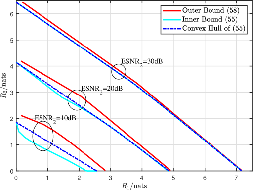
Figure 2: Bounds on capacity region of $2$-user OI-BC with average-intensity constraint.

III-C Peak- and Average-Intensity Constrained OI-BC

III-C1 Preliminary

Considering the peak- and average-intensity constraints in (4) and (5), the decomposition of a truncated exponential random variable and the existing single-user channel capacity is introduced in the following.

Lemma 7 ([33]).

Given any integer $N\in\mathbb{N}^{+}$, a truncated exponential random variable $S$, i.e.,

$$p_{S}(s)=\frac{1}{\textnormal{A}}\frac{\mu}{1-e^{-\mu}}e^{-\frac{\mu s}{\textnormal{A}}},\quad s\in[0,\textnormal{A}],\quad\mu>0,$$ (63)

can be decomposed as a sum of two independent random variables $S_{1}$ and $S_{2}$, i.e.,

$$p_{S_{1}}(s_{1}) = \frac{1}{\textnormal{A}}\frac{\mu}{1-e^{-\frac{\mu}{N}}}e^{-\frac{\mu s_{1}}{\textnormal{A}}},\quad s_{1}\in\left[0,\frac{\textnormal{A}}{N}\right],$$ (64)

$$p_{S_{2}}(s_{2}) = \frac{1-e^{-\frac{\mu}{N}}}{1-e^{-\mu}}\sum_{n=0}^{N-1}e^{-\frac{\mu n}{N}}\delta\left(s_{2}-\frac{n}{N}\times\textnormal{A}\right).$$ (65)

For convenience, the distribution in (65) is denoted by $\textsf{Texp}(\textnormal{A},\mu)$.

Lemma 8 ([10]).

The channel capacity $\mathsf{C}(\textnormal{A},\sigma;\mu^{\star})$ of a peak- and average-intensity constrained optical intensity channel is upper bounded by

$$\mathsf{C}_{\textnormal{ub}}(\textnormal{A},\sigma;\mu^{\star})=\inf_{\beta_{1}>0,\beta_{2}>0}B(\beta_{1},\beta_{2}),$$ (66)

where

$$\beta_{1} = \sigma\log\left(1+\frac{\textnormal{A}}{\sigma}\right)$$ (67)

$$\beta_{2} = \mu^{\star}\Biggl{(}1-\exp\biggl{(}-\frac{\beta_{1}^{2}}{2\sigma^{2}}\times\Bigl{(}\frac{1}{\mu^{\star}}-\frac{e^{-\mu^{\star}}}{1-e^{-\mu^{\star}}}\Bigr{)}\biggr{)}\Biggr{)},$$ (68)

and $B(\beta_{1},\beta_{2})$ is given in (66a) at the bottom of the next page. The parameter $\mu^{\star}$ is the unique solution to the following equation

$$\frac{1}{\mu^{\star}}-\frac{e^{-\mu^{\star}}}{1-e^{-\mu^{\star}}}=\alpha.$$ (69)

At high SNR,

$$\mathsf{C}_{\textnormal{ub}}(\textnormal{A},\sigma;\mu^{\star})\doteq\frac{1}{2}\log\left(1+\exp\left(2-\frac{2\mu^{\star}e^{-\mu^{\star}}}{1-e^{-\mu^{\star}}}\right)\left(\frac{1-e^{-\mu^{\star}}}{\mu^{\star}}\right)^{2}\frac{\textnormal{A}^{2}}{2\pi e\sigma^{2}}\right).$$ (70)

$$B(\beta_{1},\beta_{2})= \left(1-\mathcal{Q}\left(\frac{\beta_{1}+\left(\frac{1}{\mu^{\star}}-\frac{e^{-\mu^{\star}}}{1-e^{-\mu^{\star}}}\right)\textnormal{A}}{\sigma}\right)-\mathcal{Q}\left(\frac{\beta_{1}+(1-\left(\frac{1}{\mu^{\star}}-\frac{e^{-\mu^{\star}}}{1-e^{-\mu^{\star}}}\right))\textnormal{A}}{\sigma}\right)\right)$$

$$\times\log\left(\frac{\textnormal{A}}{\sigma}\cdot\frac{e^{\frac{\beta_{2}\beta_{1}}{\textnormal{A}}}-e^{-\beta_{2}\left(1+\frac{\beta_{1}}{\textnormal{A}}\right)}}{\sqrt{2\pi}\beta_{2}\left(1-2\mathcal{Q}\left(\frac{\beta_{1}}{\sigma}\right)\right)}\right)$$

$$-\frac{1}{2}+\mathcal{Q}\left(\frac{\beta_{1}}{\sigma}\right)+\frac{\beta_{1}}{\sqrt{2\pi}\sigma}e^{-\frac{\beta_{1}^{2}}{2\sigma^{2}}}+\frac{\sigma}{\textnormal{A}}\frac{\beta_{2}}{\sqrt{2\pi}}\left(e^{-\frac{\beta_{1}^{2}}{2\sigma^{2}}}-e^{-\frac{(\textnormal{A}+\beta_{1})^{2}}{2\sigma^{2}}}\right)$$

$$+\beta_{2}\left(\frac{1}{\mu^{\star}}-\frac{e^{-\mu^{\star}}}{1-e^{-\mu^{\star}}}\right)\left(1-2\mathcal{Q}\left(\frac{\beta_{1}+\frac{\textnormal{A}}{2}}{\sigma}\right)\right).$$ (66a)

III-C2 Bounds on Capacity Region

The inner bound on the capacity region is proposed as follows.

Theorem 7 (Inner Bound).

When the input is subject to both peak- and average-intensity constraint in (4) and (5), the rate pairs in the set $\mathsf{Conv}\{\cup_{N\in\mathbb{N}^{+}}\left(R_{1}^{\textnormal{in}}(N),R_{2}^{\textnormal{in}}(N)\right)\}$ are all achievable for a two-user OI-BC, where

$${\Hy@raisedlink{\hyper@anchorstart{\@IEEEtheHrefequation}}\Hy@raisedlink{\hyper@anchorend}}R_{1}^{\textnormal{in}}(N) = \frac{1}{2}\log\left(1+\exp\left(2-\frac{2\mu^{\star}e^{-\frac{\mu^{\star}}{N}}}{N\left(1-e^{-\frac{\mu^{\star}}{N}}\right)}\right)\left(\frac{1-e^{-\frac{\mu^{\star}}{N}}}{\mu^{\star}}\right)^{2}\frac{\textnormal{A}^{2}}{2\pi e\sigma_{1}^{2}}\right),$$ (71a)

$$R_{2}^{\textnormal{in}}(N) = \frac{1}{2}\log\left(1+\exp\left(2-\frac{2\mu^{\star}e^{-\mu^{\star}}}{1-e^{-\mu^{\star}}}\right)\left(\frac{1-e^{-\mu^{\star}}}{\mu^{\star}}\right)^{2}\frac{\textnormal{A}^{2}}{2\pi e\sigma_{2}^{2}}\right)-\mathsf{C}_{\textnormal{ub}}\left(\frac{\textnormal{A}}{N},\sigma_{2};\frac{\mu^{\star}}{N}\right).$$ (71b)

Proof.

Assume $X_{1}$ follows $\textsf{Texp}(\frac{\textnormal{A}}{N},\frac{\mu^{\star}}{N})$ and $X_{2}$ follows

$$p_{X_{2}}(x_{2}) = \frac{1-e^{-\frac{\mu^{\star}}{N}}}{1-e^{-\mu^{\star}}}\sum_{n=0}^{N-1}e^{-\frac{\mu^{\star}n}{N}}\delta\left(x_{2}-\frac{n}{N}\times\textnormal{A}\right),$$ (72)

where $N\in\mathbb{N}^{+}$. Substituting them into Lemma 7, we obtain that $X$ follows $\textsf{Texp}(\textnormal{A},\mu^{\star})$, which satisfies the peak- and average-intensity constraints in (4) and (5). Furthermore, note that $X_{1}$ satisfies $X_{1}\in[0,{\textnormal{A}}/{N}$] and $\mathbb{E}[X_{1}]=\rho\textnormal{E}$, and is independent of the Gaussian noise $Z_{2}$, thus we can bound $\mathsf{h}(X_{1}+Z_{2})$ by

$$\mathsf{h}(X_{1}+Z_{2})\leq\mathsf{C}_{\textnormal{ub}}\left(\frac{\textnormal{A}}{N},\sigma_{2};\frac{\mu^{\star}}{N}\right)+\mathsf{h}(Z_{2}).$$ (73)

Finally, following similar steps from (21) to (28), we can complete the proof.

∎

The following outer bound has been given in [26, Theorem 1]. Here, we can also utilize the conditional EPI to provide a new proof, which is similar to the proof of Theorem 2 and omitted here.

Lemma 9 (Outer Bound).

When the input is subject to both peak- and average-intensity constraints in (4) and (5), the capacity region is outer bounded by $\cup_{\rho\in[0,1]}\left(R_{1}^{\textnormal{out}}(\rho),R_{2}^{\textnormal{out}}(\rho)\right)$ for a two-user OI-BC, where

$${\Hy@raisedlink{\hyper@anchorstart{\@IEEEtheHrefequation}}\Hy@raisedlink{\hyper@anchorend}}R_{1}^{\textnormal{out}}(\rho) = \frac{1}{2}\log\left\{1+\frac{\sigma_{2}^{2}}{\sigma_{1}^{2}}\left(e^{2\mathsf{C}_{\textnormal{ub}}\left(\rho\textnormal{A},\sigma_{2};\mu^{\star}\right)}-1\right)\right\},$$ (74a)

$$R_{2}^{\textnormal{out}}(\rho) = \mathsf{C}_{\textnormal{ub}}\left(\textnormal{A},\sigma_{2};\mu^{\star}\right)-\mathsf{C}_{\textnormal{ub}}\left(\rho\textnormal{A},\sigma_{2};\mu^{\star}\right),$$ (74b)

The high-SNR capacity region is proposed as follows.

Theorem 8 (Asymptotic Capacity Region).

When the input is subject to both peak- and average-intensity constraints in (4) and (5), at high SNR, the capacity region of a two-user OI-BC asymptotically converges to the region where the rate pair $(R_{1},R_{2})$ satisfies

$${\Hy@raisedlink{\hyper@anchorstart{\@IEEEtheHrefequation}}\Hy@raisedlink{\hyper@anchorend}}R_{1} \ \dot{\leq}\ \frac{1}{2}\log\left(1+\exp\left(2-\frac{2\rho\mu^{\star}e^{-\rho\mu^{\star}}}{1-e^{-\rho\mu^{\star}}}\right)\left(\frac{1-e^{-\rho\mu^{\star}}}{\mu^{\star}}\right)^{2}\frac{\textnormal{A}^{2}}{2\pi e\sigma_{1}^{2}}\right),$$ (75a)

$$R_{2} \ \dot{\leq}\ \frac{1}{2}\log\left(\frac{\exp\left(2-\frac{2\mu^{\star}e^{-\mu^{\star}}}{1-e^{-\mu^{\star}}}\right)\left(\frac{1-e^{-\mu^{\star}}}{\mu^{\star}}\right)^{2}\textnormal{A}^{2}+2\pi e\sigma_{2}^{2}}{\exp\left(2-\frac{2\rho\mu^{\star}e^{-\rho\mu^{\star}}}{1-e^{-\rho\mu^{\star}}}\right)\left(\frac{1-e^{-\rho\mu^{\star}}}{\mu^{\star}}\right)^{2}\textnormal{A}^{2}+2\pi e\sigma_{2}^{2}}\right),$$ (75b)

with $\rho\in[0,1]$.

Proof.

The proof follows similar arguments as the proof of Theorem 3. Before that, we need to derive a new outer bound which is valid in the high SNR regime. Note that $\mathsf{h}(Y_{2}|U)$ can be bounded by

$$\mathsf{h}(Y_{2}|U) \geq \mathsf{h}(Z_{2}),$$ (76)

$$\mathsf{h}(Y_{2}|U) \leq \mathsf{C}_{\textnormal{ub}}(\textnormal{A},\sigma_{2};\mu^{\star})+\mathsf{h}(Z_{2}).$$ (77)

The function $\mathsf{C}_{\textnormal{ub}}(\rho\textnormal{A},\sigma_{2};\rho\mu^{\star})$, $\rho\in[0,1]$, is monotonically increasing with respect to $\rho$ and approaches zeros when $\rho$ tends to $0$ at high SNR. (More details about the monotonicity of $\mathsf{C}_{\textnormal{ub}}(\rho\textnormal{A},\sigma_{2};\rho\mu^{\star})$ can been found in Appendix A). Combined with (76) and (77), there exists $\rho\in[0,1]$ such that

$$\mathsf{h}(Y_{2}|U)=\mathsf{C}_{\textnormal{ub}}(\rho\textnormal{A},\sigma_{2};\rho\mu^{\star})+\mathsf{h}(Z_{2}).$$ (78)

Following similar arguments from (33) to (39), we obtain that at high SNR,

$$R_{1} \ \dot{\leq}\ \frac{1}{2}\log\left(1+\exp\left(2-\frac{2\rho\mu^{\star}e^{-\rho\mu^{\star}}}{1-e^{-\rho\mu^{\star}}}\right)\left(\frac{1-e^{-\rho\mu^{\star}}}{\mu^{\star}}\right)^{2}\frac{\textnormal{A}^{2}}{2\pi e\sigma_{1}^{2}}\right),$$ (79)

$$R_{2} \ \dot{\leq}\ \frac{1}{2}\log\left(\frac{\exp\left(2-\frac{2\mu^{\star}e^{-\mu^{\star}}}{1-e^{-\mu^{\star}}}\right)\left(\frac{1-e^{-\mu^{\star}}}{\mu^{\star}}\right)^{2}\textnormal{A}^{2}+2\pi e\sigma_{2}^{2}}{\exp\left(2-\frac{2\rho\mu^{\star}e^{-\rho\mu^{\star}}}{1-e^{-\rho\mu^{\star}}}\right)\left(\frac{1-e^{-\rho\mu^{\star}}}{\mu^{\star}}\right)^{2}\textnormal{A}^{2}+2\pi e\sigma_{2}^{2}}\right).$$ (80)

Finally, combining the above newly derived outer bound and the inner bound in Theorem 7, we can complete the proof.

∎

The derived bounds on the capacity region are shown in Fig. 3, where we assume $\sigma_{2}=2\sigma_{1}$, $\alpha=0.4$, and $\mathrm{ASNR}_{k}=\frac{\textnormal{A}}{\sigma_{k}}$, $k\in\{1,2\}$.

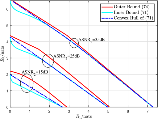
Figure 3: Bounds on capacity region of $2$-user OI-BC with peak- and average-intensity constraint when $\alpha=0.4$.

IV Capacity Region Characterization of $K$-User OI-BCs

In this section, we consider three input constraints and extend the capacity regions of two-user OI-BCs to $K$-user OI-BCs. In each case of input constraints, the inner bound is derived first and then the outer bound. Finally, the high-SNR capacity region is characterized based on these bounds.

IV-A Peak-Intensity Constrained OI-BC

The inner bound on the capacity region is derived based on the SC scheme.

Theorem 9 (Inner Bound).

When the input is only subject to the peak-intensity constraint in (4), the rate tuples in the set $\mathsf{Conv}\{\cup_{\bm{N}\in\mathfrak{D}_{\bm{N}}}\left(R_{1}^{\textnormal{in}}(\bm{N}),R_{2}^{\textnormal{in}}(\bm{N}),\cdots,R_{K}^{\textnormal{in}}(\bm{N})\right)\}$ are all achievable for a $K$-user OI-BC, where

$$R_{k}^{\textnormal{in}}(\bm{N}) = \frac{1}{2}\log\left(1+\frac{\textnormal{A}^{2}}{2\pi e(\prod_{n=k}^{K}{N}_{n})^{2}\sigma_{k}^{2}}\right)-\mathcal{C}_{\textnormal{up}}\left(\frac{\textnormal{A}}{\prod_{n=k-1}^{K}{N}_{n}},\sigma_{k}\right),\ k\in[K],\qquad$$ (81)

with $\mathfrak{D}_{\bm{N}}=\{\bm{N}=[N_{0},N_{1},\cdots,N_{K}]:{N}_{n}\in\mathbb{N}^{+},\ \forall n\in\{0\cup[K]\},\ {N}_{0}\gg 0,\ {N}_{K}=1\}$.

Proof.

We first encode the messages $M_{1}$, $M_{2}$, $\cdots$, $M_{K}$ independently into signals $X_{1}$, $X_{2}$, $\cdots$, $X_{K}$, where $X_{1}$ follows $\textsf{U}\left[0,\frac{\textnormal{A}}{\prod_{n=1}^{K}{N}_{n}}\right]$ and $\forall k\in\{2,3,\cdots,K\}$:

$$p_{X_{k}}(x_{k})=\frac{1}{{N}_{k-1}}\sum_{i=0}^{{N}_{k-1}-1}\delta\left(x_{k}-\frac{i}{{N}_{k-1}}\times\frac{\textnormal{A}}{\prod_{n=k}^{K}{N}_{n}}\right).$$ (82)

Then we adopt an SC scheme such that $X=\sum_{n=1}^{K}X_{n}$. Denote

$$X_{k,\textnormal{sum}}=\sum_{n=1}^{k}X_{n},\quad k\in[K].$$ (83)

Combined with Lemma 3, we obtain that $X_{k,\textnormal{sum}}$ follows $\textsf{U}\left[0,\frac{\textnormal{A}}{\prod_{n=k}^{K}{N}_{n}}\right]$ and $X$ follows U$[0,\textnormal{A}]$, which satisfies the peak-intensity constraint in (4). In Lemma 2, we instantiate $U_{k}$ into $U_{k}=\sum_{n=k}^{K}X_{n}$. Therefore, we can compute the achievable rate $\mathsf{I}\bigl{(}\sum_{n=k}^{K}X_{n};Y_{k}\bigm{|}\sum_{n=k+1}^{K}X_{n}\bigr{)}$ to be as the inner bounds on $R_{k}$, $k\in[K]$. To do it, we simplify $\mathsf{I}\bigl{(}\sum_{n=k}^{K}X_{n};Y_{k}\bigm{|}\sum_{n=k+1}^{K}X_{n}\bigr{)}$ as

$$\mathsf{I}\biggl{(}\sum_{n=k}^{K}X_{n};Y_{k}\biggm{|}\sum_{n=k+1}^{K}X_{n}\biggr{)} = \mathsf{I}\left(X_{k};\sum\nolimits_{n=1}^{k}X_{n}+Z_{k}\right)$$ (84)

$$= \mathsf{h}\left(\sum\nolimits_{n=1}^{k}X_{n}+Z_{k}\right)-\mathsf{h}\left(\sum\nolimits_{n=1}^{k-1}X_{n}+Z_{k}\right)$$ (85)

$$\geq \frac{1}{2}\log\left(e^{2\mathsf{h}\left(\sum\nolimits_{n=1}^{k}X_{n}\right)}+e^{2\mathsf{h}(Z_{k})}\right)-\mathsf{h}\left(\sum\nolimits_{n=1}^{k-1}X_{n}+Z_{k}\right)$$ (86)

$$\geq \frac{1}{2}\log\left(1+\frac{\textnormal{A}^{2}}{2\pi e(\prod_{n=k}^{K}{N}_{n})^{2}\sigma_{k}^{2}}\right)-\mathsf{C}_{\textnormal{ub}}\left(\frac{\textnormal{A}}{\prod_{n=k-1}^{K}{N}_{n}},\sigma_{k}\right),\quad$$ (87)

where (86) follows from the EPI; and (87) follows from the fact that $\sum\nolimits_{n=1}^{k-1}X_{n}$ is limited in $\left[\frac{\textnormal{A}}{\prod_{n=k-1}^{K}{N}_{n}}\right]$ and independent of the Gaussian noise $Z_{k}$. Combined with (87), the proof is concluded. ∎

The outer bound on the capacity region is derived based on the conditional EPI.

Theorem 10 (Outer Bound).

When the input is only subject to the peak-intensity constraint in (4), the capacity region for a $K$-user OI-BC is outer bounded by
$\cup_{\bm{\rho}\in\mathfrak{D}_{\bm{\rho}}}\left(R_{1}^{\textnormal{out}}(\bm{\rho}),R_{2}^{\textnormal{out}}(\bm{\rho}),\cdots,R_{K}^{\textnormal{out}}(\bm{\rho})\right)$, where

$$R_{k}^{\textnormal{out}}(\bm{\rho}) = \frac{1}{2}\log\left\{\frac{\sigma_{k}^{2}+\sigma_{K}^{2}\left(e^{2\mathsf{C}_{\textnormal{ub}}({\rho}_{k}\textnormal{A},\sigma_{K})}-1\right)}{\sigma_{k}^{2}+\sigma_{K}^{2}\left(e^{2\mathsf{C}_{\textnormal{ub}}({\rho}_{k-1}\textnormal{A},\sigma_{K})}-1\right)}\right\},\quad k\in[K],$$ (88)

with $\mathfrak{D}_{\bm{\rho}}=\left\{\bm{\rho}=[{\rho}_{0},{\rho}_{1},\cdots,{\rho}_{K}]:{\rho}_{k}\in[0,1],\ {\rho}_{k-1}\leq{\rho}_{k},\ \forall k\in[K],\ {\rho}_{0}=0,\ {\rho}_{K}=1\right\}$.

Proof.

We resort to Lemma 2 to derive the upper bound on the achievable rate $R_{K}$ of user $K$ first and then the achievable rates $R_{k}$s of the rest of users, $k\in[K-1]$. When $U_{K}\rightarrow X\rightarrow Y_{K}$ forms a Markov chain, it follows that

$$\mathsf{h}(Y_{K}|U_{K}) \geq \mathsf{h}(Y_{K}|X)=\mathsf{h}(Z_{K}).$$ (89)

Furthermore, we have

$$\mathsf{h}(Y_{K}|U_{K}) \leq \mathsf{h}(Y_{K})\leq\mathsf{C}_{\textnormal{ub}}(\textnormal{A},\sigma_{K})+\mathsf{h}(Z_{K}).$$ (90)

Hence, there exists ${\rho}_{K-1}\in[0,1]$ such that

$$\mathsf{h}(Y_{K}|U_{K}) = \mathsf{C}_{\textnormal{ub}}({\rho}_{K-1}\textnormal{A},\sigma_{K})+\mathsf{h}(Z_{K})$$ (91)

$$= \frac{1}{2}\log\left(2\pi e\sigma_{K}^{2}+2\pi e\sigma_{K}^{2}(e^{2\mathsf{C}_{\textnormal{ub}}({\rho}_{K-1}\textnormal{A},\sigma_{K})}-1)\right).$$ (92)

By Lemma 2, the achievable rate of user $K$ can be upper bounded by

$$R_{K} \leq \mathsf{I}(U_{K};Y_{K})$$ (93)

$$= \mathsf{h}(Y_{K})-\mathsf{h}(Y_{K}|U_{K})$$ (94)

$$\leq \mathsf{C}_{\textnormal{ub}}(\textnormal{A},\sigma_{K})+\frac{1}{2}\log\left(2\pi e\sigma_{K}^{2}\right)-\frac{1}{2}\log\left(2\pi e\sigma_{K}^{2}+2\pi e\sigma_{K}^{2}(e^{2\mathsf{C}_{\textnormal{ub}}({\rho}_{K-1}\textnormal{A},\sigma_{K})}-1)\right)$$ (95)

$$= \frac{1}{2}\log\left\{\frac{\sigma_{K}^{2}+\sigma_{K}^{2}\left(e^{2\mathsf{C}_{\textnormal{ub}}({\rho}_{K}\textnormal{A},\sigma_{K})}-1\right)}{\sigma_{K}^{2}+\sigma_{K}^{2}\left(e^{2\mathsf{C}_{\textnormal{ub}}({\rho}_{K-1}\textnormal{A},\sigma_{K})}-1\right)}\right\}.$$ (96)

Besides, the achievable rate $R_{k}$ of user $k$, $k\in[K-1]$, can be upper bounded by

$$R_{k} \leq \mathsf{I}(U_{k};Y_{k}|U_{k+1})$$ (97)

$$= \mathsf{h}(Y_{k}|U_{k+1})-\mathsf{h}(Y_{k}|U_{k}),\quad k\in[K-1],$$ (98)

where (98) holds since $U_{k+1}\rightarrow U_{k}\rightarrow Y_{k}$ forms a Markov chain. To derive an upper bound on (98), we first analyze $\mathsf{h}(Y_{k}|U_{k})$ and then $\mathsf{h}(Y_{k}|U_{k+1})$.

To analyze $\mathsf{h}(Y_{k}|U_{k})$, we assume $\forall k\in[K]$,

$$\mathsf{h}(Y_{k}|U_{k})=\frac{1}{2}\log\left(2\pi e\sigma_{k}^{2}+2\pi e\sigma_{K}^{2}(e^{2\mathsf{C}_{\textnormal{ub}}({\rho}_{k-1}\textnormal{A},\sigma_{K})}-1)\right).$$ (99)

From (92), we find that (99) is true if $k=K$. Then, we fix a particular $i\in\{2,\cdots,K\}$ and assume (99) is true if $k=i$, i.e.,

$$\mathsf{h}(Y_{i}|U_{i})=\frac{1}{2}\log\left(2\pi e\sigma_{i}^{2}+2\pi e\sigma_{K}^{2}(e^{2\mathsf{C}_{\textnormal{ub}}({\rho}_{i-1}\textnormal{A},\sigma_{K})}-1)\right).$$ (100)

We upper bound $\mathsf{h}(Y_{i-1}|U_{i-1})$ by

$$\mathsf{h}(Y_{i-1}|U_{i-1}) \leq \mathsf{h}(Y_{i-1}|U_{i})$$ (101)

$$\leq \frac{1}{2}\log\left(e^{2\mathsf{h}(Y_{i}|U_{i})}-2\pi e(\sigma_{i}^{2}-\sigma_{i-1}^{2})\right)$$ (102)

$$= \frac{1}{2}\log\left(2\pi e\sigma_{i-1}^{2}+2\pi e\sigma_{K}^{2}(e^{2\mathsf{C}_{\textnormal{ub}}({\rho}_{i-1}\textnormal{A},\sigma_{K})}-1)\right),$$ (103)

where (101) holds since $U_{i}\rightarrow U_{i-1}\rightarrow Y_{i-1}$ forms a Markov chain; (102) is obtained by substituting the conditional EPI for $Y_{i-1}+\widetilde{Z}_{i}=Y_{i}$; and (103) is obtained by substituting (100) into (102). On the other hand, since $U_{i}\rightarrow X\rightarrow Y_{i-1}$ also forms a Markov chain, we lower bound $\mathsf{h}(Y_{i-1}|U_{i-1})$ by

$$\mathsf{h}(Y_{i-1}|U_{i-1})\geq\mathsf{h}(Y_{i-1}|X)=\frac{1}{2}\log(2\pi e\sigma_{i-1}^{2}).$$ (104)

With (103) and (104), there exists ${\rho}_{i-2}\in[0,{\rho}_{i-1}]$ such that

$$\mathsf{h}(Y_{i-1}|U_{i-1})=\frac{1}{2}\log\left(2\pi e\sigma_{i-1}^{2}+2\pi e\sigma_{K}^{2}(e^{2\mathsf{C}_{\textnormal{ub}}({\rho}_{i-2}\textnormal{A},\sigma_{K})}-1)\right).$$ (105)

As a result, (99) is also true if $k=i-1$. By mathematical induction, (99) is true for $\forall k\in[K]$. To analyze $\mathsf{h}(Y_{k}|U_{k+1})$, we first note that $Y_{k}+\widetilde{Z}_{k+1}=Y_{k+1}$. By the conditional EPI, we obtain that

$$\mathsf{h}(Y_{k}|U_{k+1}) \leq \frac{1}{2}\log\left(e^{2\mathsf{h}(Y_{k+1}|U_{k+1})}-2\pi e(\sigma_{k+1}^{2}-\sigma_{k}^{2})\right)$$ (106)

$$= \frac{1}{2}\log\left(2\pi e\sigma_{k}^{2}+2\pi e\sigma_{K}^{2}(e^{2\mathsf{C}_{\textnormal{ub}}({\rho}_{k}\textnormal{A},\sigma_{K})}-1)\right),\ k\in[K-1].$$ (107)

Substituting (99) and (107) into (98), we have

$$R_{k} \leq \frac{1}{2}\log\left\{\frac{\sigma_{k}^{2}+\sigma_{K}^{2}\left(e^{2\mathsf{C}_{\textnormal{ub}}({\rho}_{k}\textnormal{A},\sigma_{K})}-1\right)}{\sigma_{k}^{2}+\sigma_{K}^{2}\left(e^{2\mathsf{C}_{\textnormal{ub}}({\rho}_{k-1}\textnormal{A},\sigma_{K})}-1\right)}\right\},\quad k\in[K-1].$$ (108)

Combining (96) and (108), we complete the proof. ∎

The high-SNR capacity region is derived based on the inner bound in Theorem 9 and the outer bound in Theorem 10. We summarize it as follows.

Theorem 11 (Asymptotic Capacity Region).

When the input is only subject to the peak-intensity constraint in (4), at high SNR, the capacity region of a $K$-user OI-BC asymptotically converges to the region where the rate tuple $(R_{1},R_{2},\cdots,R_{K})$ satisfies

$$R_{k} \ \dot{\leq}\ \frac{1}{2}\log\left(\frac{{\rho}_{k}^{2}\textnormal{A}^{2}+2\pi e\sigma_{k}^{2}}{{\rho}_{k-1}^{2}\textnormal{A}^{2}+2\pi e\sigma_{k}^{2}}\right),\quad k\in[K],$$ (109)

with $\bm{\rho}\in\mathfrak{D}_{\bm{\rho}}$ and $\mathfrak{D}_{\bm{\rho}}=\left\{\bm{\rho}:{\rho}_{k}\in[0,1],\ {\rho}_{k-1}\leq{\rho}_{k},\ \forall k\in[K],\ {\rho}_{0}=0,\ {\rho}_{K}=1\right\}$.

Proof.

Substituting the single-user capacity result in Lemma 4 into Theorem 10, we obtain that the capacity region at high SNR is outer bounded by $\cup_{\bm{\rho}\in\mathfrak{D}_{\bm{\rho}}}\left(R_{1}^{\textnormal{out}}(\bm{\rho}),R_{2}^{\textnormal{out}}(\bm{\rho}),\cdots,R_{K}^{\textnormal{out}}(\bm{\rho})\right)$, where

$$R_{k}^{\textnormal{out}}(\bm{\rho}) \doteq \frac{1}{2}\log\left(\frac{{\rho}_{k}^{2}\textnormal{A}^{2}+2\pi e\sigma_{k}^{2}}{{\rho}_{k-1}^{2}\textnormal{A}^{2}+2\pi e\sigma_{k}^{2}}\right),\quad k\in[K].$$ (110)

We write the boundary of the above outer bound as

$$R_{K}^{\textnormal{out}} \doteq \frac{1}{2}\log\left(1+\frac{\textnormal{A}^{2}}{2\pi e\sigma_{K}^{2}}\right)-\frac{1}{2}\log\left(1+\sum_{m=1}^{K-1}\frac{\sigma_{m}^{2}}{\sigma_{K}^{2}}\left(e^{2R_{m}^{\textnormal{out}}}-1\right)\prod_{n=m+1}^{K-1}e^{2R_{n}^{\textnormal{out}}}\right),\qquad$$ (111)

whose proof is given in Appendix B. The derivative of $R_{K}^{\textnormal{out}}$ is given by

$$\frac{\partial R_{K}^{\textnormal{out}}}{\partial R_{k}^{\textnormal{out}}} \doteq -\frac{\sum_{m=1}^{k-1}\frac{\sigma_{m}^{2}}{\sigma_{K}^{2}}\left(e^{2R_{m}^{\textnormal{out}}}-1\right)\prod_{n=m+1}^{K-1}e^{2R_{n}^{\textnormal{out}}}+\frac{\sigma_{k}^{2}}{\sigma_{K}^{2}}\prod_{n=k}^{K-1}e^{2R_{n}^{\textnormal{out}}}}{1+\sum_{m=1}^{K-1}\frac{\sigma_{m}^{2}}{\sigma_{K}^{2}}\left(e^{2R_{m}^{\textnormal{out}}}-1\right)\prod_{n=m+1}^{K-1}e^{2R_{n}^{\textnormal{out}}}}$$

$$= -\frac{\frac{\sigma_{1}^{2}}{\sigma_{K}^{2}}\left(e^{2R_{1}^{\textnormal{out}}}-1\right)\prod_{n=2}^{K-1}e^{2R_{n}^{\textnormal{out}}}+\sum_{m=2}^{k-1}\frac{\sigma_{m}^{2}}{\sigma_{K}^{2}}\left(e^{2R_{m}^{\textnormal{out}}}-1\right)\prod_{n=m+1}^{K-1}e^{2R_{n}^{\textnormal{out}}}+\frac{\sigma_{k}^{2}}{\sigma_{K}^{2}}\prod_{n=k}^{K-1}e^{2R_{n}^{\textnormal{out}}}}{1+\sum_{m=1}^{K-1}\frac{\sigma_{m}^{2}}{\sigma_{K}^{2}}\left(e^{2R_{m}^{\textnormal{out}}}-1\right)\prod_{n=m+1}^{K-1}e^{2R_{n}^{\textnormal{out}}}}$$

$$\doteq -\frac{\frac{\sigma_{1}^{2}}{\sigma_{K}^{2}}\frac{{\rho}_{1}^{2}\textnormal{A}^{2}}{2\pi e\sigma_{1}^{2}}\prod_{n=2}^{K-1}\frac{{\rho}_{n}^{2}}{{\rho}_{n-1}^{2}}+\sum_{m=2}^{k-1}\frac{\sigma_{m}^{2}}{\sigma_{K}^{2}}\left(\frac{{\rho}_{m}^{2}}{{\rho}_{m-1}^{2}}-1\right)\prod_{n=m+1}^{K-1}\frac{{\rho}_{n}^{2}}{{\rho}_{n-1}^{2}}+\frac{\sigma_{k}^{2}}{\sigma_{K}^{2}}\prod_{n=k}^{K-1}\frac{{\rho}_{n}^{2}}{{\rho}_{n-1}^{2}}}{1+\frac{{\rho}_{K-1}^{2}\textnormal{A}^{2}}{2\pi e\sigma_{K}^{2}}}$$ (113)

$$= -\frac{\frac{{\rho}_{K-1}^{2}\textnormal{A}^{2}}{2\pi e\sigma_{K}^{2}}+\sum_{m=2}^{k-1}\frac{\sigma_{m}^{2}}{\sigma_{K}^{2}}\left(\frac{{\rho}_{m}^{2}}{{\rho}_{m-1}^{2}}-1\right)\frac{{\rho}_{K-1}^{2}}{{\rho}_{m}^{2}}+\frac{\sigma_{k}^{2}}{\sigma_{K}^{2}}\frac{{\rho}_{K-1}^{2}}{{\rho}_{k-1}^{2}}}{1+\frac{{\rho}_{K-1}^{2}\textnormal{A}^{2}}{2\pi e\sigma_{K}^{2}}}$$ (114)

$$\doteq -1,\quad k\in[K-1],$$ (115)

where (113) follows from (110) and (149). Hence, at high SNR, the boundary of the outer bound is a $(K-1)$-dimensional hyperplane. For convenience, we denote it by $\mathcal{H}_{\textnormal{out}}$.

Next, we proceed to show that the inner bound in Theorem 9 is tight with $\mathcal{H}_{\textnormal{out}}$ at high SNR. Substituting (18) into (81), we obtain that the rate tuples in $\mathsf{Conv}\{\cup_{\bm{N}\in\mathfrak{D}_{\bm{N}}}\left(R_{1}^{\textnormal{in}}(\bm{N}),\cdots,R_{K}^{\textnormal{in}}(\bm{N})\right)\}$ are all achievable, where

$$R_{k}^{\textnormal{in}}(\bm{N}) = \frac{1}{2}\log\left(\frac{\frac{\textnormal{A}^{2}}{(\prod_{n=k}^{K}{N}_{n})^{2}}+2\pi e\sigma_{k}^{2}}{\frac{\textnormal{A}^{2}}{(\prod_{n={k-1}}^{K}{N}_{n})^{2}}+2\pi e\sigma_{k}^{2}}\right),\quad k\in[K].$$ (116)

To analyze the achievable region $\mathsf{Conv}\{\cup_{\bm{N}\in\mathfrak{D}_{\bm{N}}}\left(R_{1}^{\textnormal{in}}(\bm{N}),\cdots,R_{K}^{\textnormal{in}}(\bm{N})\right)\}$, we define a new region $\mathcal{R}$ such that

$$\mathcal{R}=\cup_{\bm{N}\in\mathfrak{D}_{\bm{N}}}\left(R_{1}^{\textnormal{in}}(\bm{N}),\cdots,R_{K}^{\textnormal{in}}(\bm{N})\right).$$ (117)

Since $\mathcal{R}\subseteq\mathsf{Conv}\{\cup_{\bm{N}\in\mathfrak{D}_{\bm{N}}}\left(R_{1}^{\textnormal{in}}(\bm{N}),\cdots,R_{K}^{\textnormal{in}}(\bm{N})\right)\}$, thus the rate tuples in $\mathcal{R}$ are also achievable. Then, we have two observations about $\mathcal{R}$. First, given any $\bm{N}\in\mathfrak{D}_{\bm{N}}$, if $\bm{\rho}$ satisfies

$${\rho}_{k}=\frac{1}{\prod_{n=k}^{K}{N}_{n}},\quad k\in\{0\cup[K]\},$$ (118)

then combined with (110) and (116), we have

$$\left(R_{1}^{\textnormal{in}}(\bm{N}),\cdots,R_{K}^{\textnormal{in}}(\bm{N})\right)\doteq\left(R_{1}^{\textnormal{out}}(\bm{\rho}),\cdots,R_{K}^{\textnormal{out}}(\bm{\rho})\right),\quad\forall\bm{N}\in\mathfrak{D}_{\bm{N}}.$$ (119)

Therefore, any achievable rate tuple in $\mathcal{R}$, is equal to some rate tuple on the hyperplane $\mathcal{H}_{\textnormal{out}}$ at high SNR, i.e., $\mathcal{R}\subseteq\mathcal{H}_{\textnormal{out}}$. Second, given any $k\in[K]$, if we let

$${N}_{k-1} \rightarrow +\infty,$$ (120)

$${N}_{n} \rightarrow 1,\quad n\in\{k,\cdots,K\},$$ (121)

then combined with (116), we can obtain that the following tuples in $\mathcal{R}$ are achievable:

$$\Bigl{(}0,\cdots,0,\underbrace{\frac{1}{2}\log\left(1+\frac{\textnormal{A}^{2}}{2\pi e\sigma_{k}^{2}}\right)}_{k},0,\cdots,0\Bigr{)},\quad k\in[K].$$ (122)

From (110), we find that these achievable rate tuples in (122) are exactly the corner points on the hyperplane $\mathcal{H}_{\textnormal{out}}$.

Now, we are ready to analyze the achievable region $\mathsf{Conv}\{\cup_{\bm{N}\in\mathfrak{D}_{\bm{N}}}\left(R_{1}^{\textnormal{in}}(\bm{N}),\cdots,R_{K}^{\textnormal{in}}(\bm{N})\right)\}$. Note that

$$\mathsf{Conv}\left\{\cup_{\bm{N}\in\mathfrak{D}_{\bm{N}}}\left(R_{1}^{\textnormal{in}}(\bm{N}),\cdots,R_{K}^{\textnormal{in}}(\bm{N})\right)\right\}=\mathsf{Conv}\left\{\mathcal{R}\right\}.$$ (123)

With the above two observations about $\mathcal{R}$, i.e., (1) $\mathcal{R}\subseteq\mathcal{H}_{\textnormal{out}}$; (2) the corner points on the hyperplane $\mathcal{H}_{\textnormal{out}}$ can be achieved by some rate tuples in $\mathcal{R}$, we conclude that $\mathsf{Conv}\left\{\cup_{\bm{N}\in\mathfrak{D}_{\bm{N}}}\left(R_{1}^{\textnormal{in}}(\bm{N}),\cdots,R_{K}^{\textnormal{in}}(\bm{N})\right)\right\}$ is also a $(K-1)$-dimensional hyperplane and overlaps with $\mathcal{H}_{\textnormal{out}}$. Hence, the inner bound in Theorem 9 and the outer bound in Theorem 10 are tight at high SNR, which completes the proof.

∎

The derived bounds on the capacity region are shown in Fig. 4, where we assume $K=3$, $\sigma_{3}=2\sigma_{2}=4\sigma_{1}$, and $\mathrm{ASNR}_{k}=\frac{\textnormal{A}}{\sigma_{k}}$, $k\in\{1,2,3\}$. In the figure, we first depict the $3$-dimensional capacity region bounds, then project the result onto $R_{2}$ and $R_{3}$ plane, $R_{2}$ and $R_{3}$ plane, and $R_{2}$ and $R_{3}$ plane, respectively. From Fig. 4, we observe that the inner and outer bounds become tighter as SNR increases, which further validates the derivations.

(a) Bounds on capacity region.

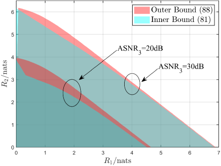
(b) Projection on the $R_{1}$ and $R_{2}$ plane.

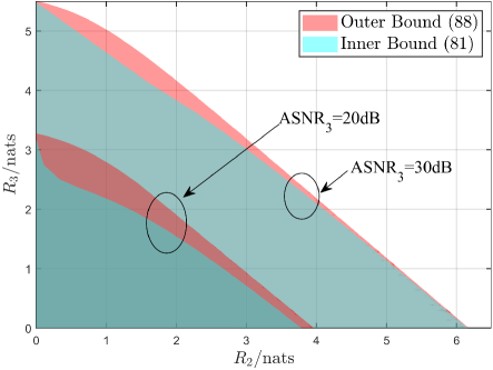
(c) Projection on the $R_{2}$ and $R_{3}$ plane.

(d) Projection on the $R_{1}$ and $R_{3}$ plane.

Figure 4: Bounds on capacity region of $3$-user OI-BC with peak-intensity constraint.

IV-B Average-Intensity Constrained OI-BC

The inner bound on the capacity region is proposed as follows.

Theorem 12 (Inner Bound).

When the input is only subject to the average-intensity constraint in (5), the rate tuples in the set $\cup_{\bm{\rho}\in\mathfrak{D}_{\bm{\rho}}}\left(R_{1}^{\textnormal{in}}(\bm{\rho}),R_{2}^{\textnormal{in}}(\bm{\rho}),\cdots,R_{K}^{\textnormal{in}}(\bm{\rho})\right)$ are all achievable for a $K$-user OI-BC, where

$$R_{k}^{\textnormal{in}}(\bm{\rho}) = \frac{1}{2}\log\left(1+\frac{e{\rho}_{k}^{2}\textnormal{E}^{2}}{2\pi\sigma_{k}^{2}}\right)-\mathsf{C}_{\textnormal{ub}}\left({\rho}_{k-1}\textnormal{E},\sigma_{k}\right),\quad k\in[K],\qquad$$ (124)

with $\mathfrak{D}_{\bm{\rho}}=\left\{\bm{\rho}=[{\rho}_{0},{\rho}_{1},\cdots,{\rho}_{K}]:{\rho}_{k}\in[0,1],\ {\rho}_{k-1}\leq{\rho}_{k},\ \forall k\in[K],\ {\rho}_{0}=0,\ {\rho}_{K}=1\right\}$.

Proof.

Assume $X_{1}$ follows $\textsf{Exp}(\rho_{1}\textnormal{E})$ and $\forall k\in\{2,3,\cdots,K\}$,

$$p_{X_{k}}(x_{k}) = \frac{{\rho}_{k-1}}{{\rho}_{k}}\delta(x_{k})+\left(1-\frac{{\rho}_{k-1}}{{\rho}_{k}}\right)\times\frac{1}{{\rho}_{k}\textnormal{E}}e^{-\frac{x_{k}}{{\rho}_{k}\textnormal{E}}},\ x_{k}\in[0,+\infty).$$ (125)

With Lemma 3, we obtain that $X_{k,\textnormal{sum}}$ in (83) follows $\textsf{Exp}(\rho_{k}\textnormal{E})$ and $X$ follows $\textsf{Exp}(\textnormal{E})$, which satisfies the average-intensity constraint in (5). Then, following similar steps in the proof of Theorem 9, we can complete the proof. ∎

We propose the outer bound on the capacity region in Theorem 13, whose proof follows similar arguments as in the proof of Theorem 10 and omitted here.

Theorem 13 (Outer Bound).

When the input is only subject to the average-intensity constraint in (5), the capacity region of a $K$-user OI-BC is outer bounded by
$\cup_{\bm{\rho}\in\mathfrak{D}_{\bm{\rho}}}\left(R_{1}^{\textnormal{out}}(\bm{\rho}),R_{2}^{\textnormal{out}}(\bm{\rho}),\cdots,R_{K}^{\textnormal{out}}(\bm{\rho})\right)$, where

$$R_{k}^{\textnormal{out}}(\bm{\rho}) = \frac{1}{2}\log\left\{\frac{\sigma_{k}^{2}+\sigma_{K}^{2}\left(e^{2\mathsf{C}_{\textnormal{ub}}({\rho}_{k}\textnormal{E},\sigma_{K})}-1\right)}{\sigma_{k}^{2}+\sigma_{K}^{2}\left(e^{2\mathsf{C}_{\textnormal{ub}}({\rho}_{k-1}\textnormal{E},\sigma_{K})}-1\right)}\right\},\quad k\in[K],$$ (126)

with $\mathfrak{D}_{\bm{\rho}}=\left\{\bm{\rho}=[{\rho}_{0},{\rho}_{1},\cdots,{\rho}_{K}]:{\rho}_{k}\in[0,1],\ {\rho}_{k-1}\leq{\rho}_{k},\ \forall k\in[K],\ {\rho}_{0}=0,\ {\rho}_{K}=1\right\}$.

The high-SNR capacity region is directly obtained by substituting the single-user capacity result in Lemma 6 into (124) and (126). We summarize it as follows.

Theorem 14 (Asymptotic Capacity Region).

When the input is only subject to the average-intensity constraint in (5), at high SNR, the capacity region of a $K$-user OI-BC asymptotically converges to the region where the rate tuple $\left({R}_{1},{R}_{2},\cdots,{R}_{K}\right)$ satisfies

$$R_{k} \ \dot{\leq}\ \frac{1}{2}\log\left(\frac{e{\rho}_{k}^{2}\textnormal{A}^{2}+2\pi\sigma_{k}^{2}}{e{\rho}_{k-1}^{2}\textnormal{A}^{2}+2\pi\sigma_{k}^{2}}\right),\quad k\in[K],$$ (127)

with $\bm{\rho}\in\mathfrak{D}_{\bm{\rho}}$ and $\mathfrak{D}_{\bm{\rho}}=\left\{\bm{\rho}:{\rho}_{k}\in[0,1],\ {\rho}_{k-1}\leq{\rho}_{k},\ \forall k\in[K],\ {\rho}_{0}=0,\ {\rho}_{K}=1\right\}$.

The derived bounds on the capacity region are shown in Fig. 5, where we assume $K=3$, $\sigma_{3}=2\sigma_{2}=4\sigma_{1}$, and $\mathrm{ESNR}_{k}=\frac{\textnormal{E}}{\sigma_{k}}$, $k\in\{1,2,3\}$.

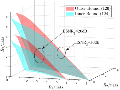
(a) Bounds on capacity region.

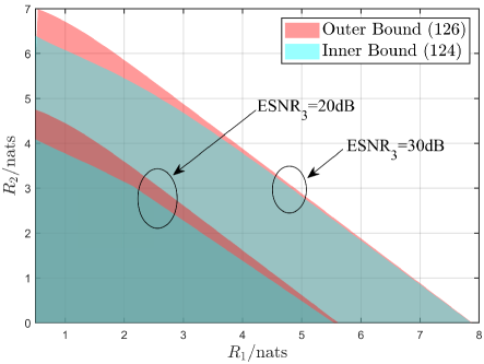
(b) Projection on the $R_{1}$ and $R_{2}$ plane.

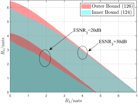
(c) Projection on the $R_{2}$ and $R_{3}$ plane.

(d) Projection on the $R_{1}$ and $R_{3}$ plane.

Figure 5: Bounds on capacity region of $3$-user OI-BC with average-intensity constraint.

IV-C Peak- and Average-Intensity Constrained OI-BC

The inner bound on the capacity region is proposed as follows.

Theorem 15 (Inner Bound).

When the input is subject to both peak- and average-intensity constraints in (4) and (5), the rate tuples in the set $\mathsf{Conv}\{\cup_{\bm{N}\in\mathfrak{D}_{\bm{N}}}\left(R_{1}^{\textnormal{in}}(\bm{N}),R_{2}^{\textnormal{in}}(\bm{N}),\cdots,R_{K}^{\textnormal{in}}(\bm{N})\right)\}$ are all achievable for a $K$-user OI-BC, where

$$R_{k}^{\textnormal{in}}(\bm{N}) = \frac{1}{2}\log\left\{1+\exp\left(2-\frac{\frac{2\mu^{\star}}{\prod_{n=k}^{K}{N}_{n}}e^{-\frac{\mu^{\star}}{\prod_{n=k}^{K}{N}_{n}}}}{1-e^{-\frac{\mu^{\star}}{\prod_{n=k}^{K}{N}_{n}}}}\right)\left(\frac{1-e^{-\frac{\mu^{\star}}{\prod_{n=k}^{K}{N}_{n}}}}{\mu^{\star}}\right)^{2}\frac{\textnormal{A}^{2}}{2\pi e\sigma_{k}^{2}}\right\}$$ (128)

$$-\mathsf{C}_{\textnormal{ub}}\left(\frac{\textnormal{A}}{\prod_{n=k-1}^{K}{N}_{n}},\sigma_{k};\frac{\mu^{\star}}{\prod_{n=k-1}^{K}{N}_{n}}\right),\quad k\in[K],\qquad$$

with $\mathfrak{D}_{\bm{N}}=\{\bm{N}=[N_{0},N_{1},\cdots,N_{K}]:{N}_{n}\in\mathbb{N}^{+},\ \forall n\in\{0\cup[K]\},\ {N}_{0}\gg 0,\ {N}_{K}=1\}$.

Proof.

Assume $X_{1}$ follows $\textsf{Texp}\left(\frac{\textnormal{A}}{\prod_{n=1}^{K}N_{n}},\frac{\mu^{\star}}{\prod_{n=1}^{K}N_{n}}\right)$ and $\forall k\in\{2,3,\cdots,K\}$,

$$p_{X_{k}}(x_{k}) = \frac{1-e^{-\frac{\frac{\mu^{\star}}{\prod_{n=k}^{K}N_{n}}}{N_{k-1}}}}{1-e^{-\frac{\mu^{\star}}{\prod_{n=k}^{K}N_{n}}}}\sum_{n=0}^{N_{k-1}-1}e^{-\frac{\frac{\mu^{\star}}{\prod_{n=k}^{K}N_{n}}n}{N_{k-1}}}\delta\left(x_{k}-\frac{n}{N_{k-1}}\times\frac{\textnormal{A}}{\prod_{n=k}^{K}N_{n}}\right).\quad$$ (129)

With Lemma 3, we obtain that $X_{k,\textnormal{sum}}$ in (83) follows $\textsf{Texp}\left(\frac{\textnormal{A}}{\prod_{n=k}^{K}N_{n}},\frac{\mu^{\star}}{\prod_{n=k}^{K}N_{n}}\right)$ and $X$ follows $\textsf{Texp}(\textnormal{A},\mu^{\star})$, which satisfies the peak- and average-intensity constraints in (4) and (5). Then, similar to the proof of Theorem 9, we can complete the proof. ∎

The following outer bound has been given in [26, Theorem 5]. We can also utilize the conditional EPI to provide a new proof, which is similar to the proof of Theorem 10 and omitted here.

Lemma 10 (Outer Bound).

When the input is subject to both peak- and average-intensity constraints in (4) and (5), the capacity region of a $K$-user OI-BC is outer bounded by $\cup_{\bm{\rho}\in\mathfrak{D}_{\bm{\rho}}}\left(R_{1}^{\textnormal{out}}(\bm{\rho}),R_{2}^{\textnormal{out}}(\bm{\rho})\right.,\cdots,$ $\left.R_{K}^{\textnormal{out}}(\bm{\rho})\right)$, where

$$R_{k}^{\textnormal{out}}(\bm{\rho}) = \frac{1}{2}\log\left\{\frac{\sigma_{k}^{2}+\sigma_{K}^{2}\left(e^{2\mathsf{C}_{\textnormal{ub}}({\rho}_{k}\textnormal{A},\sigma_{K};\mu^{\star})}-1\right)}{\sigma_{k}^{2}+\sigma_{K}^{2}\left(e^{2\mathsf{C}_{\textnormal{ub}}({\rho}_{k-1}\textnormal{A},\sigma_{K};\mu^{\star})}-1\right)}\right\},\quad k\in[K],$$ (130)

with $\mathfrak{D}_{\bm{\rho}}=\left\{\bm{\rho}=[{\rho}_{0},{\rho}_{1},\cdots,{\rho}_{K}]:{\rho}_{k}\in[0,1],\ {\rho}_{k-1}\leq{\rho}_{k},\ \forall k\in[K],\ {\rho}_{0}=0,\ {\rho}_{K}=1\right\}$.

The high-SNR capacity region is proposed as follows.

Theorem 16 (Asymptotic Capacity Region).

When the input is subject to both peak- and average-intensity constraints in (4) and (5), at high SNR, the capacity region of a $K$-user OI-BC asymptotically converges to the region where the rate tuple $\left({R}_{1},{R}_{2},\cdots,{R}_{K}\right)$ satisfies

$$R_{k} \ \dot{\leq}\ \frac{1}{2}\log\left(\frac{\exp\left(2-\frac{2\rho_{k}\mu^{\star}e^{-\rho_{k}\mu^{\star}}}{1-e^{-\rho_{k}\mu^{\star}}}\right)\left(\frac{1-e^{-\rho_{k}\mu^{\star}}}{\mu^{\star}}\right)^{2}\textnormal{A}^{2}+2\pi e\sigma_{k}^{2}}{\exp\left(2-\frac{2\rho_{k-1}\mu^{\star}e^{-\rho_{k-1}\mu^{\star}}}{1-e^{-\rho_{k-1}\mu^{\star}}}\right)\left(\frac{1-e^{-\rho_{k-1}\mu^{\star}}}{\mu^{\star}}\right)^{2}\textnormal{A}^{2}+2\pi e\sigma_{k}^{2}}\right),$$ (131)

with $\bm{\rho}\in\mathfrak{D}_{\bm{\rho}}$ and $\mathfrak{D}_{\bm{\rho}}=\left\{\bm{\rho}:{\rho}_{k}\in[0,1],\ {\rho}_{k-1}\leq{\rho}_{k},\ \forall k\in[K],\ {\rho}_{0}=0,\ {\rho}_{K}=1\right\}$.

Proof.

The proof follows similar arguments as in the proof of Theorem 11. Before that, we need to derive a new outer bound which is valid in the high SNR regime. Note that

$$\mathsf{h}(Y_{K}|U_{K}) \geq \mathsf{h}(Z_{K}),$$ (132)

$$\mathsf{h}(Y_{K}|U_{K}) \leq \mathsf{C}_{\textnormal{ub}}(\textnormal{A},\sigma_{K};\mu^{\star})+\mathsf{h}(Z_{K}).$$ (133)

At high SNR, $\mathsf{C}_{\textnormal{ub}}(\rho\textnormal{A},\sigma_{K};\rho\mu^{\star})$, $\rho\in[0,1]$, is monotonically increasing with respect to $\rho$ and approaches zeros when $\rho$ tends to $0$. Hence, there exists $\rho_{K-1}\in[0,1]$ such that

$$\mathsf{h}(Y_{K}|U_{K}) = \mathsf{C}_{\textnormal{ub}}({\rho}_{K-1}\textnormal{A},\sigma_{K};\rho_{K-1}\mu^{\star})+\mathsf{h}(Z_{K})$$ (134)

$$= \frac{1}{2}\log\left(2\pi e\sigma_{K}^{2}+2\pi e\sigma_{K}^{2}(e^{2\mathsf{C}_{\textnormal{ub}}({\rho}_{K-1}\textnormal{A},\sigma_{K};\rho_{K-1}\mu^{\star})}-1)\right).$$ (135)

Furthermore, similar to the steps from (99) to (107), we can obtain that

$$\mathsf{h}(Y_{k}|U_{k}) = \frac{1}{2}\log\left(2\pi e\sigma_{k}^{2}+2\pi e\sigma_{K}^{2}(e^{2\mathsf{C}_{\textnormal{ub}}({\rho}_{k-1}\textnormal{A},\sigma_{K};\rho_{k-1}\mu^{\star})}-1)\right),\ k\in[K-1],$$ (136)

$$\mathsf{h}(Y_{k}|U_{k+1}) \leq \frac{1}{2}\log\left(2\pi e\sigma_{k}^{2}+2\pi e\sigma_{K}^{2}(e^{2\mathsf{C}_{\textnormal{ub}}({\rho}_{k}\textnormal{A},\sigma_{K};{\rho}_{k}\mu^{\star})}-1)\right),\ k\in[K-1],$$ (137)

where $\bm{\rho}=[\rho_{1},\cdots,\rho_{K}]\in\mathfrak{D}_{\bm{\rho}}$. Then, by Lemma 2, at high SNR, we have

$$R_{k} \leq \mathsf{h}(Y_{k}|U_{k+1})-\mathsf{h}(Y_{k}|U_{k})$$ (138)

$$\ \dot{\leq}\ \frac{1}{2}\log\left(\frac{\exp\left(2-\frac{2\rho_{k}\mu^{\star}e^{-\rho_{k}\mu^{\star}}}{1-e^{-\rho_{k}\mu^{\star}}}\right)\left(\frac{1-e^{-\rho_{k}\mu^{\star}}}{\mu^{\star}}\right)^{2}\textnormal{A}^{2}+2\pi e\sigma_{k}^{2}}{\exp\left(2-\frac{2\rho_{k-1}\mu^{\star}e^{-\rho_{k-1}\mu^{\star}}}{1-e^{-\rho_{k-1}\mu^{\star}}}\right)\left(\frac{1-e^{-\rho_{k-1}\mu^{\star}}}{\mu^{\star}}\right)^{2}\textnormal{A}^{2}+2\pi e\sigma_{k}^{2}}\right),\ k\in[K].$$ (139)

Finally, combining the above newly derived outer bound and the inner bound in Theorem 15, we can complete the proof. ∎

The derived bounds on the capacity region are shown in Fig. 6, where we assume $K=3$, $\sigma_{3}=2\sigma_{2}=4\sigma_{1}$, $\alpha=0.4$, and $\mathrm{ASNR}_{k}=\frac{\textnormal{A}}{\sigma_{k}}$, $k\in\{1,2,3\}$.

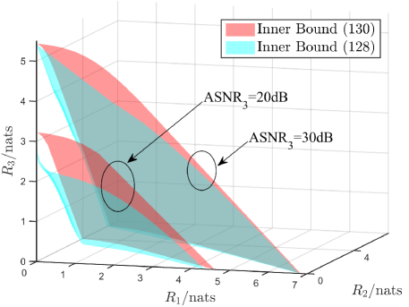
(a) Bounds on capacity region.

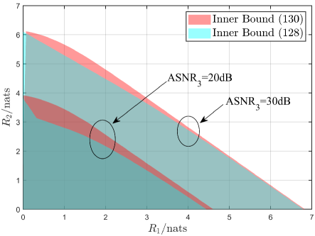
(b) Projection on the $R_{1}$ and $R_{2}$ plane.

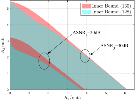
(c) Projection on the $R_{2}$ and $R_{3}$ plane.

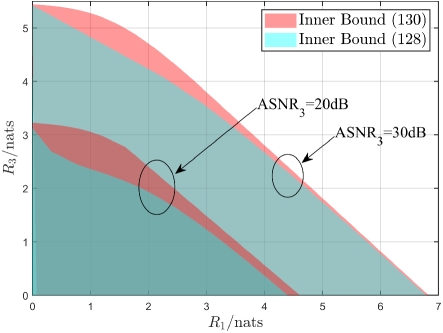
(d) Projection on the $R_{1}$ and $R_{3}$ plane.

Figure 6: Bounds on capacity region of $3$-user OI-BC with peak- and average-intensity constraint when $\alpha=0.4$.

V Conclusion Remarks

In this paper, we characterize the capacity region of OI-BCs. Three different input constraints are considered, i.e., (1) only peak-intensity constraint; (2) only average-intensity constraint; (3) both peak- and average-intensity constraints. We first consider two-user OI-BCs. New inner bounds are obtained by carefully designing the input for each user and adopting the SC scheme; new outer bounds on the capacity region are obtained by applying the conditional EPI. The inner and outer bounds asymptotically match at high SNR. Then we extend our results to the general $K$-user OI-BCs without loss of asymptotic optimality at high SNR. As an extension of this work, it would be interesting to study the impact of channel fading on the capacity region of OI-BCs, which could refer to [34, 35, 36].

Appendix A Monotonicity of $\mathsf{C}_{\textnormal{ub}}(\rho\textnormal{A},\sigma;\rho\mu)$ at High SNR

Note that at high SNR,

$$\mathsf{C}_{\textnormal{ub}}(\textnormal{A},\sigma;\mu)\doteq\frac{1}{2}\log\left(1+\exp\left(2-\frac{2\mu e^{-\mu}}{1-e^{-\mu}}\right)\left(\frac{1-e^{-\mu}}{\mu}\right)^{2}\frac{\textnormal{A}^{2}}{2\pi e\sigma^{2}}\right).$$ (140)

We denote a function $g_{1}(\rho)=\mathsf{C}_{\textnormal{ub}}(\rho\textnormal{A},\sigma;\rho\mu)$, i.e.,

$$g_{1}(\rho) = \frac{1}{2}\log\left(1+\exp\left(2-\frac{2\rho\mu e^{-\rho\mu}}{1-e^{-\rho\mu}}\right)\left(\frac{1-e^{-\rho\mu}}{\mu}\right)^{2}\frac{\textnormal{A}^{2}}{2\pi e\sigma^{2}}\right),$$ (141)

$$\qquad\qquad\qquad\qquad\rho\in[0,1],\quad\mu>0,\quad\textnormal{A}>0,\quad\sigma>0.$$

Fixed $\mu$, A, and $\sigma$, we find that the monotonicity of $g_{1}(\rho)$ is equivalent to that of the following functions:

$$g_{2}(x) =\exp\left(2-\frac{2xe^{-x}}{1-e^{-x}}\right)\times(1-e^{-x})^{2},\ x\geq 0,$$ (142)

$$g_{3}(x) =\exp\left(1-\frac{xe^{-x}}{1-e^{-x}}\right)\times(1-e^{-x}),\ x\geq 0,$$ (143)

where $g_{2}(x)=\bigl{(}g_{3}(x)\bigr{)}^{2}$. To prove that $g_{3}(x)$ is monotonically increasing with respect to $x$, we only need to analyze the following function:

$$g_{4}(x) =1-\frac{xe^{-x}}{1-e^{-x}},\quad x\geq 0$$ (144)

The derivation of $g_{4}(x)$ is given by

$$g_{4}^{\prime}(x) =\frac{xe^{-x}+e^{-2x}-e^{-x}}{(1-e^{-x})^{2}},\quad x\geq 0$$ (145)

As $x$ increases form $0$ to $+\infty$, the numerator $xe^{-x}+e^{-2x}-e^{-x}$ first increases and then decreases with respect to $x$ . Since $g_{4}^{\prime}(0)=0$ and $g_{4}^{\prime}(+\infty)=0$. Thus, wen can obtain that

$$g_{4}^{\prime}(x)\geq 0,\quad x\geq 0$$ (146)

Finally, we can conclude that $g_{1}(\rho)$ is monotonically increasing with respect to $\rho$. Equivalently, $\mathsf{C}_{\textnormal{ub}}(\rho\textnormal{A},\sigma;\rho\mu)$ is monotonically increasing with respect to $\rho$ at high SNR.

Appendix B Proof of Eq. (111)

Combined with Theorem 10, we have

$$R_{K}^{\textnormal{out}} = \frac{1}{2}\log\left(\frac{\sigma_{K}^{2}+\sigma_{K}^{2}(e^{2\mathsf{C}_{\textnormal{ub}}({\rho}_{K}\textnormal{A},\sigma_{K})}-1)}{\sigma_{K}^{2}+\sigma_{K}^{2}(e^{2\mathsf{C}_{\textnormal{ub}}({\rho}_{K-1}\textnormal{A},\sigma_{K})}-1)}\right)$$ (147)

$$\doteq \frac{1}{2}\log\left(1+\frac{\textnormal{A}^{2}}{2\pi e\sigma_{K}^{2}}\right)-\frac{1}{2}\log\left(1+\left(e^{2\mathsf{C}_{\textnormal{ub}}({\rho}_{K-1}\textnormal{A},\sigma_{K})}-1\right)\right),.$$ (148)

where (148) follows from the single-user capacity result in Lemma 4 and ${\rho}_{K}=1$. To characterize the relationship between $R_{K}^{\textnormal{out}}$ and $R_{k}^{\textnormal{out}}$, $k\in[K-1]$, we assume

$$e^{2\mathsf{C}_{\textnormal{ub}}({\rho}_{k}\textnormal{A},\sigma_{K})}-1\doteq\sum_{m=1}^{k}\frac{\sigma_{m}^{2}}{\sigma_{K}^{2}}\left(e^{2R_{m}^{\textnormal{out}}}-1\right)\prod_{n=m+1}^{k}e^{2R_{n}^{\textnormal{out}}},\quad k\in[K-1].$$ (149)

We resort to mathematical induction to prove (149). Recall that

$$R_{1}^{\textnormal{out}} = \frac{1}{2}\log\left(\frac{\sigma_{1}^{2}+\sigma_{K}^{2}(e^{2\mathsf{C}_{\textnormal{ub}}({\rho}_{1}\textnormal{A},\sigma_{K})}-1)}{\sigma_{1}^{2}+\sigma_{K}^{2}(e^{2\mathsf{C}_{\textnormal{ub}}({\rho}_{0}\textnormal{A},\sigma_{K})}-1)}\right)$$ (150)

$$\doteq \frac{1}{2}\log\left(1+\frac{\sigma_{K}^{2}}{\sigma_{1}^{2}}\left(e^{2\mathsf{C}_{\textnormal{ub}}({\rho}_{1}\textnormal{A},\sigma_{K})}-1\right)\right).$$ (151)

Then we have

$$e^{2\mathsf{C}_{\textnormal{ub}}({\rho}_{1}\textnormal{A},\sigma_{K})}-1 \doteq \frac{\sigma_{1}^{2}}{\sigma_{K}^{2}}\left(e^{2R_{1}^{\textnormal{out}}}-1\right).$$ (152)

Hence, (149) is true if $k=1$. Next, we fix a particular $i\in\{1,\cdots,K-2\}$ and assume (149) is true if $k=i$, i.e.,

$$e^{2\mathsf{C}_{\textnormal{ub}}({\rho}_{i}\textnormal{A},\sigma_{K})}-1 \doteq \sum_{m=1}^{i}\frac{\sigma_{m}^{2}}{\sigma_{K}^{2}}\left(e^{2R_{m}^{\textnormal{out}}}-1\right)\prod_{n=m+1}^{i}e^{2R_{n}^{\textnormal{out}}},$$ (153)

It follows that

$$R_{i+1}^{\textnormal{out}} \doteq \frac{1}{2}\log\left(\frac{\sigma_{i+1}^{2}+\sigma_{K}^{2}(e^{2\mathsf{C}_{\textnormal{ub}}({\rho}_{i+1}\textnormal{A},\sigma_{K})}-1)}{\sigma_{i+1}^{2}+\sigma_{K}^{2}\sum_{m=1}^{i}\frac{\sigma_{m}^{2}}{\sigma_{K}^{2}}\left(e^{2R_{m}^{\textnormal{out}}}-1\right)\prod_{n=m+1}^{i}e^{2R_{n}^{\textnormal{out}}}}\right),$$ (154)

and

$$e^{2\mathsf{C}_{\textnormal{ub}}({\rho}_{i+1}\textnormal{A},\sigma_{K})}-1 \doteq e^{2R_{i+1}^{\textnormal{out}}}\times\left(\frac{\sigma_{i+1}^{2}}{\sigma_{K}^{2}}+\sum_{m=1}^{i}\frac{\sigma_{m}^{2}}{\sigma_{K}^{2}}\left(e^{2R_{m}^{\textnormal{out}}}-1\right)\prod_{n=m+1}^{i}e^{2R_{n}^{\textnormal{out}}}\right)-\frac{\sigma_{i+1}^{2}}{\sigma_{K}^{2}}$$ (155)

$$= \sum_{m=1}^{i+1}\frac{\sigma_{m}^{2}}{\sigma_{K}^{2}}\left(e^{2R_{m}^{\textnormal{out}}}-1\right)\prod_{n=m+1}^{i+1}e^{2R_{n}^{\textnormal{out}}}.$$ (156)

Therefore, (149) is also true if $k=i+1$. Finally, by mathematical induction, we conclude that (149) holds for every $k\in[K-1]$.

Substituting (149) into (148), the relationship between $R_{K}^{\textnormal{out}}$ and $R_{k}^{\textnormal{out}}$, $k\in[K-1]$, can be characterized by

$$R_{K}^{\textnormal{out}} \doteq \frac{1}{2}\log\left(1+\frac{\textnormal{A}^{2}}{2\pi e\sigma_{K}^{2}}\right)-\frac{1}{2}\log\left(1+\sum_{m=1}^{K-1}\frac{\sigma_{m}^{2}}{\sigma_{K}^{2}}\left(e^{2R_{m}^{\textnormal{out}}}-1\right)\prod_{n=m+1}^{K-1}e^{2R_{n}^{\textnormal{out}}}\right),\quad$$ (157)

which concludes the proof.

References

- [1] P. Yang, Y. Xiao, M. Xiao and S. Li, “6G wreless communications: Vision and potential techniques,” IEEE Netw., vol. 33, no. 4, pp. 70-75, Jul. 2019.
- [2] M. Giordani, M. Polese, M. Mezzavilla, S. Rangan and M. Zorzi, “Toward 6G networks: Use cases and technologies,” IEEE Commun. Mag., vol. 58, no. 3, pp. 55-61, Mar. 2020.
- [3] M. Z. Chowdhury, M. Shahjalal, S. Ahmed and Y. M. Jang, “6G wireless communication systems: Applications, requirements, technologies, challenges, and research directions,” IEEE Open J. Commun. Soc., vol. 1, pp. 957-975, Jul. 2020.
- [4] M. A. Khalighi and M. Uysal, “Survey on free space optical communication: A communication theory perspective,” IEEE Commun. Surv. Tutor., vol. 16, no. 4, pp. 2231-2258, Fourthquarter 2014.
- [5] H. Kaushal and G. Kaddoum, “Optical communication in space: Challenges and mitigation techniques,” IEEE Commun. Surv. Tutor., vol. 19, no. 1, pp. 57-96, Firstquarter 2017.
- [6] P. H. Pathak, X. Feng, P. Hu and P. Mohapatra, “Visible light communication, networking, and sensing: A survey, potential and challenges,” IEEE Commun. Surv. Tutor., vol. 17, no. 4, pp. 2047-2077, Fourthquarter 2015.
- [7] D. Karunatilaka, F. Zafar, V. Kalavally, and R. Parthiban, “LED based indoor visible light communications: State of the art,” IEEE Commun. Surveys Tutor., vol. 17, no. 3, pp. 1649–1678, 3rd Quart., 2015.
- [8] C. Cox, E. Ackerman, R. Helkey and G. E. Betts, “Direct-detection analog optical links,” IEEE Trans. Microw Theory and Tech., vol. 45, no. 8, pp. 1375-1383, Aug. 1997.
- [9] S. C. J. Lee, S. Randel, F. Breyer and A. M. J. Koonen, “PAM-DMT for intensity-modulated and direct-detection optical communication systems,” IEEE Photon. Technol. Lett., vol. 21, no. 23, pp. 1749-1751, Dec. 2009.
- [10] A. Lapidoth, S. M. Moser and M. A. Wigger, “On the capacity of free-space optical intensity channels,” IEEE Trans. Inf. Theory, vol. 55, no. 10, pp. 4449-4461, Oct. 2009.
- [11] A. Chaaban, J. -M. Morvan and M. -S. Alouini, “Free-space optical communications: Capacity bounds, approximations, and a new sphere-packing perspective,” IEEE Trans. on Commun., vol. 64, no. 3, pp. 1176-1191, Mar. 2016.
- [12] J. Zhou and W. Zhang, “On the capacity of bandlimited optical intensity channels with Gaussian noise,” IEEE Trans. Commun., vol. 65, no. 6, pp. 2481-2493, Jun. 2017.
- [13] A. Chaaban, Z. Rezki and M. -S. Alouini, “Fundamental limits of parallel optical wireless channels: Capacity results and outage formulation,” IEEE Trans. Commun., vol. 65, no. 1, pp. 296-311, Jan. 2017.
- [14] T. Fath and H. Haas, “Performance comparison of MIMO techniques for optical wireless communications in indoor environments,” IEEE Trans. Commun., vol. 61, no. 2, pp. 733-742, Feb. 2013.
- [15] M. Uysal and H. Nouri, “Optical wireless communications—An emerging technology,” in Proc. 16th Int. Conf. Transparent Opt. Netw. (ICTON), Jul. 2014, pp. 1–7.
- [16] Z. Ghassemlooy, S. Arnon, M. Uysal, Z. Xu and J. Cheng, “Emerging optical wireless communications-advances and challenges,” IEEE J. Sel. Areas Commun., vol. 33, no. 9, pp. 1738-1749, Sept. 2015.
- [17] V. W. S. Chan, “Free-space optical communications,” J. Light. Technol., vol. 24, no. 12, pp. 4750-4762, Dec. 2006.
- [18] T. Komine and M. Nakagawa, “Fundamental analysis for visible-light communication system using LED lights,” IEEE Trans. Consum. Electron., vol. 50, no. 1, pp. 100-107, Feb. 2004.
- [19] H. Elgala, R. Mesleh and H. Haas, “Indoor optical wireless communication: Potential and state-of-the-art,” IEEE Commun. Mag., vol. 49, no. 9, pp. 56-62, Sept. 2011.
- [20] A. L. McKellips, “Simple tight bounds on capacity for the peak-limited discrete time channel,” in Proc. IEEE Int. Symp. Inf. Theory, Chicago, IL, USA, Jun. 27–Jul. 2, 2004, p. 348.
- [21] S. Hranilovic and F. R. Kschischang, “Capacity bounds for power- and band-limited optical intensity channels corrupted by Gaussian noise,” IEEE Trans. Inf. Theory, vol. 50, no. 5, pp. 784-795, May 2004.
- [22] A. A. Farid and S. Hranilovic, “Capacity bounds for wireless optical intensity channels with Gaussian noise,” IEEE Trans. Inf. Theory, vol. 56, no. 12, pp. 6066-6077, Dec. 2010.
- [23] A. Chaaban, Z. Rezki and M. -S. Alouini, “Low-SNR asymptotic capacity of MIMO optical intensity channels with peak and average constraints,” IEEE Trans. Commun., vol. 66, no. 10, pp. 4694-4705, Oct. 2018.
- [24] L. Li, S. M. Moser, L. Wang, and M. Wigger, “On the capacity of MIMO optical wireless channels,” IEEE Trans. Inf. Theory, vol. 66, no. 9, pp. 5660–5682, Oct. 2020.
- [25] A. E. Gamal and Y.-H. Kim, Network Information Theory, Cambridge, U.K.: Cambridge Univ. Press, 2011.
- [26] A. Chaaban, Z. Rezki, and M. S. Alouini, “On the capacity of the intensity-modulation direct-detection optical broadcast channel,” IEEE Trans. Wireless Commun., vol. 15, no. 5, pp. 3114–3130, Jan. 2016.
- [27] A. Chaaban, O. M. S. Al-Ebraheemy, T. Y. Al-Naffouri, and M.-S. Alouini, “Capacity bounds for the gaussian IM-DD optical multiple-access channel,” IEEE Trans. Wireless Commun., vol. 16, no. 5, pp. 3328–3340, Mar. 2017.
- [28] J. Zhou and W. Zhang, “Bounds on the capacity region of the optical intensity multiple access channel,” IEEE Trans. Commun., vol. 67, no. 11, pp. 7629–7641, Aug. 2019.
- [29] Z. Zhang and A. Chaaban, “Capacity bounds for the two-user IM/DD interference channel,” IEEE Trans. Commun., vol. 70, no. 9, pp. 5960-5974, Sept. 2022.
- [30] S. Verdu and Dongning Guo, “A simple proof of the entropy-power inequality,” IEEE Trans. Inf. Theory, vol. 52, no. 5, pp. 2165-2166, May 2006.
- [31] T. M. Cover and J. A. Thomas, Elements of Information Theory, 2nd ed. New York, NY, USA: Wiley, 2006.
- [32] C. Nair and Z. V. Wang, “The capacity region of the three receiver less noisy broadcast channel,” IEEE Trans. Inf. Theory, vol. 57, no. 7, pp. 4058-4062, Jul. 2011.
- [33] L. Li, R. -H. Chen, J. Zhou, “On the sum-capacity of two-user optical intensity multiple access channels”, arXiv preprint arXiv:2211.06691, 2022.
- [34] X. Zhu and J. M. Kahn, “Free-space optical communication through atmospheric turbulence channels,” IEEE Trans. Commun., vol. 50, no. 8, pp. 1293-1300, Aug. 2002.
- [35] E. Bayaki, R. Schober and R. K. Mallik, “Performance analysis of MIMO free-space optical systems in gamma-gamma fading,” IEEE Trans. Commun., vol. 57, no. 11, pp. 3415-3424, Nov. 2009.
- [36] F. Yang, J. Cheng and T. A. Tsiftsis, “Free-space optical communication with nonzero boresight pointing errors,” IEEE Trans. Commun., vol. 62, no. 2, pp. 713-725, Feb. 2014.