A Unified Momentum-based Paradigm of Decentralized SGD for Non-Convex Models and Heterogeneous Data

Abstract

Emerging distributed applications recently boost the development of decentralized machine learning, especially in IoT and edge computing fields. In real-world scenarios, the common problems of non-convexity and data heterogeneity result in inefficiency, performance degradation, and development stagnation. The bulk of studies concentrates on one of the issues mentioned above without having a more general framework that has been proven optimal. To this end, we propose a unified paradigm called UMP, which comprises two algorithms D-SUM and GT-DSUM based on the momentum technique with decentralized stochastic gradient descent (SGD). The former provides a convergence guarantee for general non-convex objectives, while the latter is extended by introducing gradient tracking, which estimates the global optimization direction to mitigate data heterogeneity (i.e., distribution drift). We can cover most momentum-based variants based on the classical heavy ball or Nesterov’s acceleration with different parameters in UMP. In theory, we rigorously provide the convergence analysis of these two approaches for non-convex objectives and conduct extensive experiments, demonstrating a significant improvement in model accuracy up to $57.6\%$ compared to other methods in practice.

1 Introduction

Distributed machine learning (DML) has emerged as an important paradigm in large-scale machine learning Wan et al. (2022); Zhang et al. (2022); Qu et al. (2022). In terms of how to aggregate the model parameters/gradients among workers, researchers classify the system architecture into two main classes: parameter server (PS) and decentralized. The former is generally considered as the centralized paradigm where the central server acts as a coordinator for convenience, while the latter allows communication in a peer-to-peer fashion over an underlying topology, which could guarantee the model consistency across all workers with better scalability.

Meanwhile, multiple complementary studies Fang et al. (2018); Yu et al. (2019); Hsieh et al. (2020) have focused on the issues of DML mainly based on the following two key aspects. $\bullet$ The property of non-convex objectives is quite complicated in deep learning, in particular in distributed scenarios Karimireddy et al. (2020); Lian et al. (2017). Although some standard theoretical results have been obtained for convex models Tao et al. (2022); Deng and Gao (2021); Tao et al. (2021), much less is applicable in non-convex settings since they may be lossy and cause serious obstacles (e.g., high computation complexity and poor generalization) Ghadimi et al. (2015); Mai and Johansson (2020). $\bullet$ It is well known that heterogeneity in the data is one of key challenges in distributed training, resulting in a slow and unstable convergence as well as poor model generalization. There still exists a gap between the disappointing empirical performance and the degree of data heterogeneity Shang et al. (2022); Lin et al. (2021); Esfandiari et al. (2021). Unfortunately, there are currently no existing works attempting to improve real-world decentralized training from a comprehensive perspective by taking both non-convexity and data heterogeneity into account. Thus, it is non-trivial to handle these challenges, which significantly hinder the development of real-life applications.

Motivated by the momentum’s effects on optimal convergence complexity and empirical evaluation successes  Koloskova et al. (2019); Yu et al. (2019); Han and Gao (2021); Lin et al. (2021), we propose UMP, a Unified, Momentum-based Paradigm in the decentralized learning without considering the communication overhead throughout the paper. It consists of two algorithms named D-SUM and GT-DSUM. The former one D-SUM explores the potential of momentum by maintaining and scaling the momentum buffer to sharpen the loss landscape significantly and overcomes the restrictions of non-convexity, leading to better model performance and faster convergence rate in the non-convex settings. Our latter algorithm GT-DSUM also aims to mitigate the impact of data heterogeneity on the discrepancy of local model parameters by introducing the gradient tracking (GT) technique Di Lorenzo and Scutari (2016). The core insight is that the variance between workers is decreasing while the local gradient asymptotically aligns with the global optimization direction independent on the heterogeneity of the data. GT-DSUM accelerates decentralized learning achieving better generalization performance under both non-convex and different degrees of non-IID.

This paper makes the following main contributions:

• We propose a unified momentum-based paradigm UMP with two algorithms for dealing with non-convex and the degree of non-IID simultaneously. Moreover, a variety of algorithms with the momentum technique could be obtained by specifying the parameters of our base algorithms.

• We design the first algorithm D-SUM, which achieves good model performance, demonstrating its applicability in terms of efficacy and efficiency. We also provide its convergence result under the non-convex cases.

• Our second one GT-DSUM, which is robust to the distribution drift problem by applying the GT technique, is being further developed. We rigorously prove its convergence bound in smooth, non-convex settings.

• We additionally conduct extensive experiments to evaluate the performance of UMP on common models, datasets, and dynamic real-world settings. Experimental results demonstrate that D-SUM and GT-DSUM improve the model accuracy by up to $35.8\%$ and $57.6\%$ respectively under different non-IID degrees compared with the well-known decentralized baselines. GT-DSUM performs better than D-SUM on model generalization across training tasks suffering from data skewness.

2 The Unified Paradigm: UMP

In this section, we first begin with the notation and revisit two momentum approaches: the heavy ball (HB) method Polyak (1964) and Nesterov’s momentum Nesterov (1983). Inspired by them, we generalize a unified momentum-based paradigm with two algorithms D-SUM and GT-DSUM, which could cover the above two classical methods and other momentum-based variants, aiming to address issues on non-convexity and data heterogeneity in real-world decentralized learning applications. Finally, we provide the convergence result that they could converge almost to a stationary point for general smooth, non-convex objectives.

2.1 Notation and Preliminary

To better demonstrate the applicable effect in real-world complex scenarios, we consider a decentralized setting with a network topology where $n$ workers jointly deal with an optimization problem. Assume that for every worker $i$, it holds its own datasets drawn from $\mathcal{D}_{i}$ distribution, which corresponds to data heterogeneity. Let $f_{i}:\mathbb{R}^{d}\to\mathbb{R}$ be the training datasets loss function of worker $i$ and can be given in a stochastic form $\mathbb{E}_{\xi_{i}\sim\mathcal{D}_{i}}\left[\nabla F_{i}(\mathbf{x},\xi_{i})\right]=\nabla f_{i}(\mathbf{x})$, where $F_{i}(\mathbf{x},\xi_{i})$ is the per-data loss function related with the mini-batch sample $\xi_{i}\sim\mathcal{D}_{i}$. Then, we formulate the empirical risk minimization with sum-structure objectives:

$$f^{\ast}=\min_{\mathbf{x}\in\mathbb{R}^{d}}\left[f(\mathbf{x}):=\frac{1}{n}\sum_{i=1}^{n}\left[f_{i}(\mathbf{x})=\mathbb{E}_{\xi_{i}\sim\mathcal{D}_{i}}F_{i}(\mathbf{x},\xi_{i})\right]\right].$$ (1)

Among workers, there is an underlying topology graph $\mathbf{W}\in\mathbb{R}^{n\times n}$, which is convenient to encode the communication between arbitrary two workers, i.e., we let $w_{ij}=0$ if and only if worker $i$ and $j$ are not connected.

Definition 1 (Consensus Matrix  Koloskova et al. (2021)).

A matrix with non-negative entries $\mathbf{W}\in\left[0,1\right]^{n\times n}$ that is symmetric ($\mathbf{W}=\mathbf{W}^{\top}$), and doubly stochastic ($\mathbf{W1}=\mathbf{1},\mathbf{1}^{\top}\mathbf{W}=\mathbf{1}$), where $\mathbf{1}$ denotes the all-one vector in $\mathbb{R}^{n}$.

Throughout the paper, we use the notation $\mathbf{x}_{i}^{(t),\tau}$ to denote the sequence of model parameters on worker $i$ at the $\tau$-th local update in epoch $t$. For any vector $\mathbf{a}_{i}\in\mathbb{R}^{d}$, we denote its model averaging $\bar{\mathbf{a}}=\frac{1}{n}\sum_{i=1}^{n}\mathbf{a}_{i}$. Let $\left\|\cdot\right\|$, $\left\|\cdot\right\|_{F}$ denote the $l_{2}$ vector norm and Frobenius matrix norm, respectively.

For ease of presentation, we apply both vector and matrix notation whenever it is more convenient. We denote by a capital letter for the matrix form combining by $\mathbf{a}_{i}$ as follows,

$$\begin{matrix}\mathbf{A}=\left[\mathbf{a}_{1},\cdots,\mathbf{a}_{n}\right]\in\mathbb{R}^{d\times n},&\bar{\mathbf{A}}=\left[\bar{\mathbf{a}},\cdots,\bar{\mathbf{a}}\right]=\mathbf{A}\frac{1}{n}\mathbf{11}^{\top}.\end{matrix}$$ (2)

The introduction of a momentum term is one of the most common modifications, which is viewed as a critical component for training the state-of-the-art deep neural networks Qu et al. (2022); Lin et al. (2021). Corresponding to its empirical success, momentum attempts to enhance the convergence rate on non-convex objectives by setting the optimized searching direction as the combination of stochastic gradient and historical directions.

The HB method (i.e., also known as Polyak’s momentum) is first proposed for the smooth and convex settings, written as

$$\left\{\begin{matrix}\begin{aligned} &\mathbf{u}_{i}^{(t+1)}=\beta\mathbf{u}_{i}^{(t)}+\mathbf{g}_{i}^{(t)}\\ &\mathbf{x}_{i}^{(t+1)}=\mathbf{x}_{i}^{(t)}-\eta\mathbf{u}_{i}^{(t+1)},\end{aligned}\end{matrix}\right.$$ (3)

where $\mathbf{u}_{i}^{(t)}$, $\mathbf{g}_{i}^{(t)}$ are denoted as the momentum buffer, and the stochastic gradient of worker $i$ at epoch $t$, respectively. $\eta$ presents the learning rate. The momentum variable $\beta$ adjusts the magnitude of updating direction provided by the past information estimation with the stochastic gradient, indicating the direction of the steepest descent. Equivalently, (3) can be also updated below

$$\mathbf{x}_{i}^{(t+1)}=\mathbf{x}_{i}^{(t)}-\eta\mathbf{g}_{i}^{(t)}+\beta\left(\mathbf{x}_{i}^{(t)}-\mathbf{x}_{i}^{(t-1)}\right),$$ (4)

when $t\geq 1$. Holding the past gradient values, this style of update can have better stability to some extent and enables improvement compared with some vanilla SGD methods Cutkosky and Mehta (2020).

Another kind of technique called Nesterov’s shows that choosing with suitable parameters, the extrapolation step can be accelerated from $\mathcal{O}\left(\frac{1}{t}\right)$ to $\mathcal{O}\left(\frac{1}{t^{2}}\right)$, which is the optimal rate for the smooth convex problems. Concretely, its update step is described as follows

$$\left\{\begin{matrix}\begin{aligned} &\mathbf{u}_{i}^{(t+1)}=\beta\mathbf{u}_{i}^{(t)}+\mathbf{g}_{i}^{(t)}\\ &\mathbf{v}_{i}^{(t+1)}=\beta\mathbf{u}_{i}^{(t+1)}+\mathbf{g}_{i}^{(t)}\\ &\mathbf{x}_{i}^{(t+1)}=\mathbf{x}_{i}^{(t)}-\eta\mathbf{v}_{i}^{(t+1)}.\end{aligned}\end{matrix}\right.$$ (5)

The model parameters are updated by introducing the momentum vector $\mathbf{u}_{i}$ and extra auxiliary $\mathbf{v}_{i}$ sequences. Compared with (3), through decaying the momentum buffer $\mathbf{u}_{i}^{(t)}$, it effectively improves the rate of convergence without causing oscillations. Similarly, the above steps can be written as

$$\mathbf{x}_{i}^{(t+1)}=\mathbf{x}_{i}^{(t)}-\eta\mathbf{g}_{i}^{(t)}+\beta\left(\mathbf{x}_{i}^{(t)}-\eta\mathbf{g}_{i}^{(t)}-\mathbf{x}_{i}^{(t-1)}+\eta\mathbf{g}_{i}^{(t-1)}\right).$$ (6)

Based on (4) and (6), it is not difficult to observe that the former could evaluate the gradient and add momentum simultaneously, while the latter applies momentum after evaluating gradients, which intuitively causes more computation cost. Meanwhile, leveraging the idea of HB momentum, Nesterov’s acceleration brings us closer to the minimum (i.e., $\mathbf{x}^{\ast}$) by introducing an additional gradient descent rule by adding the subtracted gradients $\eta(\mathbf{g}_{i}^{(t-1)}-\mathbf{g}_{i}^{(t)})$ for general convex cases. The above two basic momentum-based approaches are firstly investigated in convex settings, showing their advantage compared with the vanilla SGD. However, there is still a shortage of a comprehensive analysis of momentum-based SGD under non-convex conditions in common real-world scenarios.

2.2 D-SUM Algorithm

Input: $\forall i$, initialize $\mathbf{x}_{i}^{(0),0}=\mathbf{v}_{i}^{(0),0}=\mathbf{x}_{0}$; constant parameters $\eta$, $\alpha$, and $\beta$; $\forall i,j$, consensus matrix $\mathbf{W}$ with entries $w_{ij}$; the number of epochs $T$ and local steps $K$.

1 for $t\in\left\{0,\cdots,T-1\right\}$ at worker $i$ in parallel do

2       Set $\mathbf{x}_{i}^{(t),0}=\mathbf{x}_{i}^{(t)},\mathbf{v}_{i}^{(t),0}=\mathbf{v}_{i}^{(t)}$.

3       for $\tau\in\left\{0,\cdots,K-1\right\}$  do

4             Sample $\xi_{i}^{(t),\tau}$ and compute $\mathbf{g}_{i}^{(t),\tau}=\nabla F_{i}(\mathbf{x}_{i}^{(t),\tau},\xi_{i}^{(t),\tau})$.

5             $\mathbf{x}^{(t),\tau+1}=\mathbf{x}^{(t),\tau}-\eta\mathbf{g}_{i}^{(t),\tau}$.

6             Compute local model $\mathbf{x}_{i}^{(t),\tau}$ from (7).

7            

8       end for

9      Perform gossip averaging via (8).

10       $\mathbf{v}_{i}^{(t+1)}=\sum_{j=1}^{n}w_{ij}\mathbf{v}_{j}^{(t),K}$.

11      

12 end for

Algorithm 1 vanilla SGD and D-SUM; colors indicate the two alternative variants.

In this section, we present UMP and its first algorithm D-SUM, which is employed in decentralized training under non-convex cases.

Under each epoch, workers first perform $K$ local updates using different optimizers (i.e., SGD, Adam  Kingma and Ba (2015), etc.) with or without momentum. In this paper, we mainly focus on the momentum-based SGD variants, which are demonstrated in (3), and (5) for example. From a comprehensive view, we apply the key update of the stochastic unified momentum (SUM) is according to

$$\left\{\begin{matrix}\begin{aligned} &\mathbf{u}_{i}^{(t),\tau+1}=\mathbf{x}_{i}^{(t),\tau}-\eta\mathbf{g}_{i}^{(t),\tau}\\ &\mathbf{v}_{i,}^{(t),\tau+1}=\mathbf{x}_{i}^{(t),\tau}-\alpha\eta\mathbf{g}_{i}^{(t),\tau}\\ &\mathbf{x}_{i}^{(t),\tau+1}=\mathbf{u}_{i}^{(t),\tau+1}+\beta\left(\mathbf{v}_{i}^{(t),\tau+1}-\mathbf{v}_{i}^{(t),\tau}\right),\end{aligned}\end{matrix}\right.$$ (7)

where $\alpha\geq 0$, and $\beta\in\left[0,1\right)$. $\mathbf{a}_{i}^{(t),\tau}$ ($\mathbf{a}_{i}$ could be the instance for $\mathbf{x}_{i}$, $\mathbf{u}_{i}$, $\mathbf{v}_{i}$, and $\mathbf{g}_{i}$) is denoted as the related variables for worker $i$ after $\tau$ local updates in epoch $t$. After $K$ local steps, worker $i$ communicates with its neighbors according to the communication pattern $\mathbf{W}$ for exchanging their local model parameters. We call this synchronization operation as gossip averaging which can be compactly written as

$$\mathbf{x}_{i}^{(t+1)}=\sum_{j=1}^{n}w_{ij}\mathbf{x}_{j}^{(t),K}.$$ (8)

To present the difference between vanilla SGD and stochastic unified momentum in (7), we summarize the training procedure in Algorithm 1. The specific algorithm instance is obtained by tuning the hyperparameters $\alpha$, $\beta$, $\eta$, and $K$. We cover the basic Heavy Ball method (4) and Nesterov’s momentum (6) when setting $\alpha=0$, and $\alpha=1$, respectively. Besides, when $K=1$, it reduces to the standard mini-batch SGD with momentum acceleration. Specially, we update the auxiliary variable sequences $\left\{\mathbf{v}_{i}\right\}$ for any worker $i$ by using the same gossip synchronization as in (8) interpreted as a restart in the next training epoch to simplify theoretical analysis.

However, there is no theoretical or empirical analysis to demonstrate that the momentum gets rid of heterogeneity which degrades the distributed deep training due to the discrepancies between local activation statistics Hsieh et al. (2020). Not only taking non-convex functions into account, but we also incorporate a technique that is agnostic to data heterogeneity, gradient tracking into D-SUM to alleviate the impact of heterogeneous data in decentralized training for better model generalization in the following.

2.3 GT-DSUM Algorithm

Input: $\forall i$, initialize $\mathbf{x}_{i}^{(0),0}=\mathbf{v}_{i}^{(0),0}=\mathbf{x}_{0}$, $\mathbf{y}_{i}^{(0)}=\mathbf{g}_{i}^{(0),0}=\nabla F_{i}(\mathbf{x}_{i}^{(0),0},\xi_{i}^{(0),0})$, and $\mathbf{d}_{i}^{(-1)}=\mathbf{0}_{p}$; constant parameters $\alpha\geq 0,\beta\in\left[0,1\right),\eta,\lambda\in\left[0,1\right]$; $\forall i,j$, consensus matrix $\mathbf{W}$ with entries $w_{ij}$; the number of epochs $T$, and local steps $K$.

1 for $t\in\left\{0,\cdots,T-1\right\}$ at worker $i$ in parallel do

2       for $\tau\in\left\{0,\cdots,K-1\right\}$ do

3             Sample $\xi_{i}^{(t),\tau}$, compute $\mathbf{g}_{i}^{(t),\tau}=\nabla F_{i}(\mathbf{x}_{i}^{(t),\tau},\xi_{i}^{(t),\tau})$.

4             $\mathbf{m}_{i}^{(t),\tau}=\lambda\mathbf{g}_{i}^{(t),\tau}+(1-\lambda)\mathbf{y}_{i}^{(t)}$.

5             Substitute $\mathbf{g}_{i}^{(t),\tau}$ with $\mathbf{m}_{i}^{(t),\tau}$ as the local gradient estimation, perform (7).

6            

7       end for

8      Gossip averaging $\mathbf{x}_{i}^{(t+1)}=\sum_{j=1}^{n}w_{ij}\mathbf{x}_{j}^{(t),K}$.

9       $\mathbf{v}_{i}^{(t+1)}=\sum_{j=1}^{n}w_{ij}\mathbf{v}_{i}^{(t),K}$.

10       $\mathbf{d}_{i}^{(t)}=\frac{\mathbf{x}_{i}^{(t)}-\mathbf{x}_{i}^{(t+1)}}{K\eta}$.

11       Gradient tracking based on $\mathbf{y}_{i}^{(t+1)}=\sum_{j=1}^{n}w_{ij}\left(\mathbf{y}_{j}^{(t)}+\mathbf{d}_{j}^{(t)}-\mathbf{d}_{j}^{(t-1)}\right)$.

12      

13 end for

Algorithm 2 GT-DSUM

In this subsection, we go further the fact that heterogeneity hinders the local momentum acceleration  Lin et al. (2021) and provides our second algorithm in UMP, termed GT-DSUM, which aims to generalize the consensus model parameters better and alleviate the impact of heterogeneous data by applying the gradient tracking technique.

Taking the discrepancies between workers’ local data partition into account, GT introduces an extra worker-sided auxiliary variable $\mathbf{y}_{i}^{(t)},\forall i$ aiming to asymptotically track the average of $\nabla f_{i}$ assuming the local accurate gradients are accessible at any epoch $t$. Intuitively, GT is agnostic to the heterogeneity, while $\mathbf{y}_{i}^{(t)}$ is approximately equivalent to the global gradient direction along with the epoch $t$ increases. Inspired by this, we introduce GT into D-SUM, yields GT-DSUM. Concretely, we normalize the applied gradient $\mathbf{m}_{i}^{(t),\tau}$ using the mini-batch gradient $\mathbf{g}_{i}^{(t),\tau}$, and the $\mathbf{y}_{i}^{(t)}$ with the dampening factor $\lambda$ to highlight the necessity of local updates. The detailed algorithm is described in Algorithm 2. Within local updates, the model parameters are updated on line 5 with D-SUM but using a normalization term $\mathbf{m}_{i}^{(t),\tau}$. Line 7 and 8 are the same as the basic D-SUM procedures in Algorithm 1. For GT-DSUM, we apply the difference of two consecutive synchronized models shown in line 9 to update the gradient tracker variable in line 10 using the gossip-liked style Xin et al. (2021b, a). Especially, when $K=1$, $\lambda=1$ and $\beta=0$, the Algorithm 2 can be reduced to the original GT algorithm  Koloskova et al. (2021) instance.

Since Algorithm 1 and 2 employ multiple consensus steps from parameters exchanging which significantly increase communication cost, we apply the communication compression technique GRACE Xu et al. (2021) to trade off between model generalization and communication overhead in Section 3.

2.4 Theoretical Analysis

In what follows, we present the convergence analysis of two algorithms in the UMP for general non-convex settings. The detailed proof is in Appendix. Firstly, we state our assumptions throughout the paper.

Assumption 1 ($L$-smooth).

For each function $f_{i}:\mathbb{R}^{d}\to\mathbb{R}$ is differentiable, and there exists a constant $L>0$ such that for each $\mathbf{x},\mathbf{x}^{\prime}\in\mathbb{R}^{d}:\left\|\nabla f(\mathbf{x})-\nabla f(\mathbf{x}^{\prime})\right\|\leq L\left\|\mathbf{x}-\mathbf{x}^{\prime}\right\|$.

Assumption 2 (Bounded variances).

We assume that there exists $\sigma>0$ and $\zeta>0$ for any $i,\mathbf{x}\in\mathbb{R}^{d}$ such that $\mathbb{E}_{\xi_{i}\sim\mathcal{D}_{i}}\left\|\nabla F_{i}(\mathbf{x},\xi_{i})-\nabla f_{i}(\mathbf{x})\right\|^{2}\leq\sigma^{2}$, and $\frac{1}{n}\sum_{i=1}^{n}\left\|\nabla f_{i}(\mathbf{x})-\nabla f(\mathbf{x})\right\|^{2}\leq\zeta^{2}$.

Assumptions 1 and 2 are standard in general non-convex objective literature Lin et al. (2021); Yu et al. (2019); Koloskova et al. (2020) in order to ensure the basis of loss functions continuous and the limited influence of heterogeneity among distributed scenarios. Noted that when $\zeta=0$, we have $\nabla f_{i}(\mathbf{x})=\nabla f(\mathbf{x})$, i.e., it reduces to the case of IID data distribution across all participating workers. The third common assumption is to assume the stochastic gradients are uniformly bounded which is stated as follows.

Assumption 3 (Bounded stochastic gradient).

We assume that the second moment of stochastic gradients is bounded for any $i,\mathbf{x}\in\mathbb{R}^{d},\mathbb{E}_{\xi_{i}\sim\mathcal{D}_{i}}\left\|\nabla F_{i}(\mathbf{x},\xi_{i})\right\|^{2}\leq G^{2}$.

Assumption 4.

The mixing matrix is doubly stochastic by Definition 1. Further, define $\bar{\mathbf{Z}}=\mathbf{Z}\frac{1}{n}\mathbf{11}^{\top}$ for any matrix $\mathbf{Z}\in\mathbb{R}^{d\times n}$. Then, the mixing matrix satisfies $\mathbb{E}_{\mathbf{W}}\left\|\mathbf{ZW}-\bar{\mathbf{Z}}\right\|^{2}_{F}\leq(1-\rho)\left\|\mathbf{Z}-\bar{\mathbf{Z}}\right\|^{2}_{F}$.

In Assumption 4, we assume that $\rho:=1-\max\left\{\left|\lambda_{2}(\mathbf{W})\right|,\left|\lambda_{n}(\mathbf{W})\right|\right\}^{2}>0$, where let $\lambda_{i}(\mathbf{W})$ denote the $i$-th largest eigenvalue of the mixing matrix $\mathbf{W}$ with $-1\leq\lambda_{n}(\mathbf{W})\leq\cdots\leq\lambda_{2}(\mathbf{W})\leq\lambda_{1}(\mathbf{W})\leq 1$. For example, the value of $\rho$ is commonly used when $\rho=1$ for the full-mesh (complete) communication topology.

2.4.1 Convergence Analysis of D-SUM

We now state our convergence result for D-SUM (red highlight) in Algorithm 1. The detailed proof is presented in Appendix B

Theorem 1.

Considering problem (1) under the above mentioned assumptions, we denote $\beta_{0}=\max\left\{1+\beta,1+\alpha\beta\right\}$, for all $T\geq 1$ and $K\geq 1$ in Algorithm 1 with learning rate $\eta\leq\frac{\rho}{5L}$ and parameters satisfy $\frac{4-\rho}{2}<\frac{1}{\beta_{0}^{2}}$, we have

$$\frac{1}{KT}\sum_{t=0}^{T-1}\sum_{\tau=0}^{K-1}\mathbb{E}\left\|\nabla f(\bar{\mathbf{x}}^{(t),\tau})\right\|^{2}$$

$$\quad\leq\frac{2\left(f(\mathbf{x}_{0})-f^{\ast}\right)}{\tilde{\eta}KT}+\frac{2\beta^{2}\hat{\eta}^{2}L^{2}G^{2}}{n(1-\beta)^{4}}+\frac{2L^{2}C_{1}}{n^{2}(1-Q_{1})}$$

$$\quad\quad+\frac{L}{n}\left(\sigma^{2}+2\tilde{\eta}G^{2}+3\sigma^{2}\tilde{\eta}\right),$$

where $\tilde{\eta}=\frac{\eta}{1-\beta}$, $\hat{\eta}=\left((1-\beta)\alpha-1\right)\eta$, $Q_{1}=2\beta_{0}^{2}(1-\frac{\rho}{4})$, and $C_{1}=24\eta^{2}\beta_{0}^{2}\zeta^{2}/\rho+4\left(1-\rho\right)\left(1+2\alpha\beta+2\alpha^{2}\beta^{2}\right)\eta^{2}\sigma^{2}$.

Remark 1.

Theorem 1 proposes a non-asymptotic convergence bound of D-SUM for general neural network since the second term i.e., $\mathcal{O}\left(\frac{L^{2}\hat{\eta}^{2}}{n}\right)$ generates from the core SGD step in (7). Intuitively, there exists an appropriate $\alpha$ for achieving the optimal training performance in practice, which has been observed in the single node case Yan et al. (2018). In Section 3, we perform related experiments to confirm this speculation.

2.4.2 Convergence Analysis of GT-DSUM

Next theorem is the convergence result of GT-DSUM in Algorithm 2 when $K=1$ with a fixed communication topology among workers for convenience, and the detailed proof is in Appendix C. Based on the GT is addressed with the issue on how to apply the mini-batch gradient estimates to track the global optimization descent direction, we define the following proposition to clarify this illustration.

Proposition 1 (Gradients averaging tracker Di Lorenzo and Scutari (2016)).

We assume a loose constraint that the auxiliary variables $\mathbf{y}_{i}^{(t)}$ are considered as the tracker of the average $\frac{1}{n}\sum_{j=1}^{n}\nabla f_{j}(\mathbf{x}_{i}^{(t)})$, which means for any epoch $t$, we have $\mathbb{E}\left\|\mathbf{y}_{i}^{(t)}-\frac{1}{n}\sum_{j=1}^{n}\nabla f_{j}(\mathbf{x}_{i}^{(t)})\right\|^{2}\leq\epsilon^{2}$.

Theorem 2.

Consider problem (1) under the listed specific assumptions, we denote $\beta_{0}=\max\left\{1+\alpha\beta,1+\beta\right\}$, and set $T\geq 1$ in Algorithm 2 without multiple local steps (i.e., $K=1$) with learning rate $\eta$ chosen as

$$0\leq\eta\leq\min\left\{\frac{\rho}{12\lambda},\frac{1-\beta}{2},\frac{3+\beta}{2\sqrt{3}\lambda(1+\alpha\beta)},\frac{1+\beta}{2\sqrt{3}\lambda\alpha\beta}\right\}\frac{1}{L}$$

and parameters satisfy

$$\left\{\begin{matrix}\begin{aligned} &(1+\alpha\beta)(1-\lambda)\leq\frac{1}{2\sqrt{2}},\\ &\rho\leq\frac{48\lambda^{2}L^{2}}{(1-\lambda)^{2}},\\ &4\beta_{0}^{2}\left(1-\frac{\rho}{4}\right)<1,\\ &8(1-\rho)(1+\alpha\beta)^{2}<1,\end{aligned}\end{matrix}\right.$$

we have

$$\frac{1}{T}\sum_{t=0}^{T-1}\mathbb{E}\left\|\nabla f(\bar{\mathbf{x}}^{(t)})\right\|^{2}$$

$$\leq\frac{2\left(f(\mathbf{x}_{0})-f^{\ast}\right)}{\tilde{\eta}T}+\frac{8\beta^{2}\hat{\eta}^{2}L^{2}}{n(1-\beta)^{4}}\left(\sigma^{2}+3\zeta^{2}+4G^{2}\right)$$

$$\quad+\frac{12L^{2}}{n}\left(\frac{Q_{3}}{T}+\frac{(2-Q_{2})Q_{4}}{(1-Q_{2})T}+\frac{V_{\max}}{1-Q_{2}}+\frac{C_{2}}{1-Q_{2}}\right)$$

$$\quad+\frac{4\lambda^{2}\sigma^{2}+16\zeta^{2}}{n}+8(1-\lambda^{2})\epsilon^{2}+\frac{12\beta^{2}\hat{\eta}^{2}L^{2}\epsilon^{2}}{(1-\beta)^{4}}$$

where $\tilde{\eta}=\frac{\eta}{1-\beta}$ and $\hat{\eta}=(\alpha-\alpha\beta-1)\eta$. In addition, $C_{2}=\frac{\beta_{0}^{2}\left(1-\frac{\rho}{2}\right)}{L^{2}}(\sigma^{2}+\zeta^{2})(192\lambda^{2}L^{2}+\rho)$, $Q_{2}\triangleq\min\left\{4\beta_{0}^{2}\left(1-\frac{\rho}{4}\right),8(1-\rho)(1+\alpha\beta)^{2}\right\}$, $Q_{3}=6(\zeta^{2}+\sigma^{2})$, $Q_{4}=\beta_{0}^{2}\left(1-\frac{\rho}{2}\right)(\sigma^{2}+\zeta^{2})\left(48+\frac{\rho}{L^{2}}+192\lambda^{2}\right)$. Furthermore, we define $V_{\max}\triangleq\max_{0\leq t\leq T-1}\left\{\frac{1}{n}\left(\mathbb{E}\left\|\mathbf{X}^{(t)}-\bar{\mathbf{X}}^{(t)}\right\|_{F}^{2}+\mathbb{E}\left\|\mathbf{Y}^{(t)}-\bar{\mathbf{Y}}^{(t)}\right\|_{F}^{2}\right)\right\}.$

Remark 2.

The fourth term on the right-hand side of the Theorem 2, i.e., $\mathcal{O}\left(\frac{1}{nT}+\frac{\beta_{0}^{2}}{nT}+\frac{1}{n\beta_{0}^{2}}\right)$ comes from the the additional GT step for searching global optimal descent estimation in line $10$, Algorithm 2. However, this term can be dominant when $\alpha$ scales due to its higher order. Clearly, $\beta_{0}=1+\alpha\beta$ when $\alpha>1$, and it performs the convergence rate $\mathcal{O}\left(\frac{\beta_{0}^{2}}{nT}\right)$, leading to a significant deterioration from convergence perspective if $\alpha$ rises. Hence, we will show the impact of $\alpha$ in Section 3.

3 Evaluation

Our main evaluation results demonstrate that D-SUM outperforms other methods in terms of model accuracy, and GT-DSUM achieves a higher performance under different levels of non-IID. All experiments are executed in a CPU/GPU cluster, equipped with Inter(R) Xeon(R) Gold 6126, 4 GTX 2080Ti cards, and 12 Tesla T4 cards. We used Pytorch and Ray Moritz et al. (2018) to implement and train our models.

3.1 Experiment Methodology

Baselines. We consider the following three decentralized methods with momentum, which are described as follows: $\bullet$ Local SGD Stich (2018) periodically averages model parameters among all worker nodes. Compared with the vanilla SGD, each node independently runs the single-node SGD with Heavy Ball momentum. $\bullet$ QG-DSGDm Lin et al. (2021) mimics the global optimization direction and integrates the quasi-global momentum into local stochastic gradients without causing extra communication costs. It empirically mitigates the impact on data heterogeneity. $\bullet$ SlowMo Wang et al. (2020) performs a slow, periodical momentum update through an All-Reduce pattern (model averaging) after multiple SGD steps. For simplicity, we use the common mini-batch gradient as the local update direction.

Datasets and models. We study the decentralized behaviors on both computer vision (CV) and natural language processing (NLP) tasks, including MNIST, EMNIST, CIFAR10, and AG NEWS. For all CV tasks, we train different CNN models. For NLP, we train an RNN, which includes an embedding layer, and a dropout layer, followed by a dense layer. The model description is shown in Appendix D.

Table 1: The testing accuracy with different algorithms on various training benchmarks and different degrees of non-IID.

Datasets	Algorithms	Testing Accuracy ($\%$)
		non-IID $=0.1$	non-IID $=1$	non-IID $=10$
MNIST LeCun et al. (1998)	Local SGD w/ momentum	$95.66\pm 0.21$	$97.99\pm 0.03$	$98.39\pm 0.03$
	QG-DSGDm	$96.02\pm 0.19$	$97.46\pm 1.36$	$98.21\pm 0.04$
	SlowMo	$97.32\pm 0.02$	$97.93\pm 0.07$	$98.34\pm 0.06$
	D-SUM (ours)	$\textbf{97.89}\pm 0.21$	$\textbf{98.77}\pm 0.04$	$\textbf{98.94}\pm 0.01$
	GT-DSUM (ours)	$97.51\pm 0.61$	$98.70\pm 0.01$	$98.82\pm 0.03$
EMNIST Cohen et al. (2017)	Local SGD w/ momentum	$45.90\pm 1.21$	$36.77\pm 0.13$	$38.29\pm 0.03$
	QG-DSGDm	$46.03\pm 0.6$	$46.02\pm 0.12$	$36.72\pm 0.02$
	SlowMo	$45.52\pm 0.03$	$37.11\pm 0.01$	$37.50\pm 0.0$
	D-SUM (ours)	$49.68\pm 0.43$	$49.75\pm 0.05$	$42.50\pm 0.01$
	GT-DSUM (ours)	$\textbf{50.49}\pm 0.82$	$\textbf{50.25}\pm 0.07$	$\textbf{51.87}\pm 0.02$
CIFAR10 Krizhevsky et al. (2009)	Local SGD w/ momentum	$22.94\pm 1.11$	$42.93\pm 0.85$	$52.82\pm 0.01$
	QG-DSGDm	$26.34\pm 1.42$	$49.12\pm 038$	$54.03\pm 0.24$
	SlowMo	$31.06\pm 1.27$	$50.46\pm 0.04$	$55.50\pm 0.10$
	DSUM (ours)	$31.16\pm 1.27$	$54.34\pm 0.11$	$57.59\pm 1.05$
	GT-DSUM (ours)	$\textbf{36.16}\pm 0.74$	$\textbf{56.95}\pm 1.56$	$\textbf{59.34}\pm 1.55$
AG NEWS Zhang et al. (2015)	Local SGD w/ momentum	$75.51\pm 0.44$	$77.98\pm 0.39$	$80.66\pm 0.02$
	QG-DSGDm	$78.82\pm 0.31$	$79.33\pm 0.38$	$82.24\pm 0.02$
	SlowMo	$82.57\pm 0.03$	$83.17\pm 0.01$	$83.79\pm 0.01$
	DSUM (ours)	$84.13\pm 0.55$	$85.46\pm 0.31$	$87.52\pm 0.04$
	GT-DSUM (ours)	$\textbf{84.29}\pm 0.37$	$\textbf{87.59}\pm 0.18$	$\textbf{89.07}\pm 0.04$

Hyperparameters. For all algorithms with different benchmarks, the setting deploys $10$ workers by default. In our experiments, we set the local mini-batch size as $256$ for CIFAR10 and $128$ for the rest, and the number of local updates is set as $K=10$. To illustrate the challenge of data heterogeneity in decentralized deep training, we adopt the Dirichlet distribution value Lin et al. (2021) to control different levels of non-IID degree, for the case with non-IID $=0.1,1,10$; the smaller the value is, the more likely the workers hold samples from only one class of labels (i.e., non-IID $=0.1$ can be viewed as an extreme data skewness case). Besides, we set the scalar $\alpha$, momentum $\beta$, normalized parameter $\lambda$ as $2$, $0.9$, and $0.8$ respectively by default. Among choices of $\mathbf{W}$ considered in practice, we pre-construct a dynamic topology changing sequence varying from full-mesh to ring by the popular Metropolis-Hastings rule Koloskova et al. (2021) i.e., $w_{ij}=w_{ji}=\min\left\{\frac{1}{\text{deg}(i)+1},\frac{1}{\text{deg}(j)+1}\right\}$ for any $i,j$, $w_{ii}=1-\sum_{j=1}^{n}w_{ij}$. The learning rate $\eta$ is fine-tuned via a grid search on the set $\left\{10^{-2},10^{-1.5},10^{-1},10^{-0.5}\right\}$ for each algorithm and dataset.

Performance Metrics. We examine the effects of different momentum variants on decentralized deep learning, including

• Model generalization is measured by the proportion between the amount of the correct data by the model and that of all data in the test dataset. We report the averaged model performance of local models over test samples.

• Effect of different hyperparameters is explored by tuning their values to study the properties of D-SUM and GT-DSUM.

• Scalability is a crucial property while handling tasks in a distributed situation.

3.2 Evaluation results

Performance with compared baselines. In Table 1, we can see that our proposed algorithms outperform all other baselines across different levels of data skewness. For CIFAR10 and AG NEWS, the performance of our algorithms and benchmarks: GT-DSUM $>$ D-SUM $>$ SlowMo $>$ QG-DSGDm $>$ Local SGD w/ momentum. Our proposed algorithms outperform other benchmarks on model generalization and demonstrate that GT technique effectively mitigates the negative impact caused by data heterogeneity. As the non-IID level increases, GT-DSUM achieves a higher accuracy than Local SGD w/ momentum up to $57.6\%$ on CIFAR10.

Table 2: The impact of $\alpha$ for D-SUM and GT-DSUM on the test accuracy with non-IID $=1$. “$\star$” indicates non-convergence.

Datasets	Methods	The test accuracy ($\%$) evaluated on different $\alpha$ under the non-IID $=1$ case
		$\alpha=0$	$\alpha=0.5$	$\alpha=1$	$\alpha=2$	$\alpha=3$	$\alpha=4$	$\alpha=5$	$\alpha=8$	$\alpha=10$	$\alpha=15$
MNIST	D-SUM	$98.05$	$98.40$	$98.57$	$98.76$	$98.85$	$98.76$	$98.85$	99.09	$98.87$	$92.86$
	GT-DSUM	$98.18$	$98.50$	$98.70$	$98.70$	98.80	$\star$	$\star$	$\star$	$\star$	$\star$
EMNIST	D-SUM	$37.1$	$43.58$	$35.58$	$49.75$	55.32	$49.80$	$43.00$	$48.47$	$53.04$	$\star$
	GT-DSUM	$33.72$	$46.06$	$47.10$	50.25	$39.84$	$\star$	$\star$	$\star$	$\star$	$\star$
CIFAR10	D-SUM	$47.10$	$50.85$	$51.68$	$50.32$	54.83	$51.10$	$51.53$	$50.68$	$\star$	$\star$
	GT-DSUM	$45.98$	$49.80$	$50.55$	$54.77$	57.58	$54.43$	$\star$	$\star$	$\star$	$\star$
AG NEWS	D-SUM	$79.16$	$81.78$	$83.72$	$85.46$	$86.38$	$86.36$	$88.20$	$87.07$	88.82	$88.56$
	GT-DSUM	$78.90$	$83.12$	$85.34$	87.59	$86.89$	$77.67$	$\star$	$\star$	$\star$	$\star$

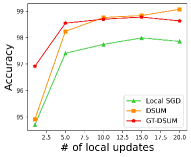
(a) LeNet over MNIST

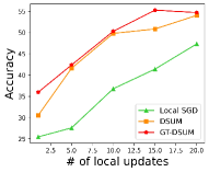
(b) CNN over EMNIST

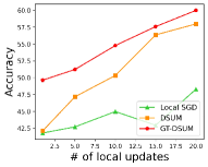
(c) LeNet over CIFAR10

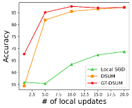
(d) RNN over AG NEWS

Figure 1: Impact on the number of local updates $K$ on the convergence when momentum $\beta=0.9$ under the non-IID $=1$ case.

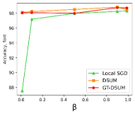
(a) LeNet over MNIST

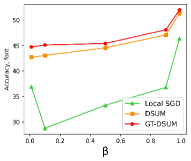
(b) CNN over EMNIST

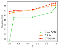
(c) LeNet over CIFAR10

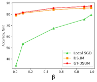
(d) RNN over AG NEWS

Figure 2: Impact on the momentum $\beta$ on the convergence when the number of local update $K=10$ under the non-IID $=1$ case.

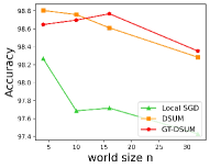
(a) LeNet over MNIST

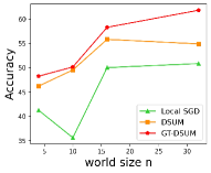
(b) CNN over EMNIST

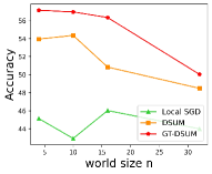
(c) LeNet over CIFAR10

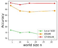
(d) RNN over AG NEWS

Figure 3: Impact on the momentum world size on the convergence when the number of local update $K=10$ under the non-IID $=1$ case.

Effect of local update. The number of local updates $K$ is one of the most important parameters since it influences the final model generalization and training time. As usual, the number of $K$ is set less than $20$ Reddi et al. (2020); Qu et al. (2022). Hence, we present the comparison with $K\in\left\{1,5,10,15,20\right\}$. We make two observations from the results in Figure 1. Firstly, our algorithms have better performance than Local SGD w/ momentum regardless $K$. For CIFAR10 and AG NEWS, shown in Figure 1(c), 1(d), we observe that GT-DSUM always keep competitive when the number of local updates increases. Among them, it improves accuracy $53.8\%$ than Local SGD w/ momentum when $K=5$. Secondly, we can find see that the workers may not guarantee to improve the model generalization substantially by increasing the number of local updates $K$. Besides, all benchmarks perform worst when $K=1$, while when $K$ is too large, performance may be degraded because workers’ local models drift too far apart in distributed optimizations Qu et al. (2022).

Effect of $\beta$. The momentum term $\beta$ is further investigated via grid search on the set $\left\{0,01,0.1,0.5,0.9,0.99\right\}$ as different strategies for handling algorithms. The third set of simulations evaluates the performance of model accuracy on different $\beta$, which are depicted in Figure 2. We have a key observation from those results. Regardless of datasets or models, evaluation results with a greater $\beta$ (e.g., 0.9, 0.99) trend to outperform with a smaller one (e.g., 0.01, 0.1). In addition, it can be observed that the testing accuracy monotonically increases with $\beta$ on CIFAR10 and AG NEWS. We note that GT-DSUM reaches a higher model accuracy compared with Local SGD w/ momentum when $\beta$ is increasing. Among all tasks, it improves test accuracy up to $56.8\%$ than Local SGD w/ momentum.

Sensitivity of $\alpha$. One of the most important parameters $\alpha$ is varying from $0$ to $15$ to analyze its influence on the convergence performance. Two observations are as follows according to Table 2. Firstly, we note that different optimal values of $\alpha$ are always found when D-SUM is evaluated on various datasets with the same level of data heterogeneity (e.g., non-IID $=1$). It is hard and time-consuming to determine the optimum $\alpha$ due to different characteristics of datasets and models. Secondly, as $\alpha$ increases, GT-DSUM makes a significant degradation on model performance. This phenomenon verifies the analysis detailed in Remark 2, which indicates that GT-DSUM requires a stricter constraint on $\alpha$ than D-SUM to ensure model validity. Empirically, there is still a gap between the vulnerable property of $\alpha$ to the momentum-based optimizer and the robustness endowing with a superior performance.

Scalability. We finally train on different numbers of workers compared with Local SGD w/ momentum when non-IID $=1$. We evaluate this by extending the scale by adjusting the number of devices $n$ training on $4$, $10$, $16$, and $32$ workers. Results are shown in Figure 3. When the number of participating workers increases, the advantage of our schemes is readily apparent since our method GT-DSUM consistently reaches a higher model accuracy compared to the Local SGD w/ momentum in this non-IID case.

4 Conclusion

In this paper, we propose a unified momentum-based paradigm UMP with two algorithms D-SUM and GT-DSUM. The former obtains good model generalization, dealing with the validity under non-convex cases, while the latter is further developed by applying the GT technique to eliminate the negative impact of heterogeneous data. By deriving the convergence of general non-convex settings, these algorithms achieve competitive performance closely related to a critical parameter $\alpha$. Extensive experimental results show our UMP leads to at most $57.6\%$ increase in improvement of accuracy.

Appendix A Prerequisite

For giving the theoretical analysis of the convergence results of all proposed algorithms, we first present some preliminary facts as follows:

• Fact 1: For any random vector $\mathbf{a}$, it holds for $\mathbb{E}\left\|\mathbf{a}\right\|^{2}=\mathbb{E}\left\|\mathbf{a}-\mathbb{E}\left[\mathbf{a}\right]\right\|^{2}+\left\|\mathbb{E}\left[\mathbf{a}\right]\right\|^{2}$.

• Fact 2: For any $a>0$, we have $\pm\left\langle\mathbf{a},\mathbf{b}\right\rangle\leq\frac{1}{2a}\left\|\mathbf{a}\right\|^{2}+\frac{a}{2}\left\|\mathbf{b}\right\|^{2}$.

• Fact 3: $\left\langle\mathbf{a},\mathbf{b}\right\rangle=\frac{1}{2}\left\|\mathbf{a}\right\|^{2}+\frac{1}{2}\left\|\mathbf{b}\right\|^{2}-\frac{1}{2}\left\|\mathbf{a}-\mathbf{b}\right\|^{2}$.

• Fact 4: For given two vectors $\mathbf{a}$ and $\mathbf{b},\forall a>0$, we have $\left\|\mathbf{a}+\mathbf{b}\right\|^{2}\leq(1+a)\left\|\mathbf{a}\right\|^{2}+(1+\frac{1}{a})\left\|\mathbf{b}\right\|^{2}$.

• Fact 5: For arbitrary set of $n$ vectors $\left\{\mathbf{a}_{i}\right\}_{i=1}^{n}$, we have $\left\|\sum_{i=1}^{n}\mathbf{a}_{i}\right\|^{2}\leq n\sum_{i=1}^{n}\left\|\mathbf{a}_{i}\right\|^{2}$.

• Fact 6: Suppose $\left\{b_{i}\right\}_{i=1}^{n}$, and $\left\{\mathbf{a}_{i}\right\}_{i=1}^{n}$ are a set of non-negative scalars and vectors, respectively. We define $s=\sum_{i=1}^{n}b_{i}$. Then according to Jensen’s inequality, we have $\left\|\sum_{i=1}^{n}b_{i}\mathbf{a}_{i}\right\|^{2}=s^{2}\left\|\sum_{i=1}^{n}\frac{b_{i}}{s}\mathbf{a}_{i}\right\|^{2}\leq s^{2}\cdot\sum_{i=1}^{n}\frac{b_{i}}{s}\left\|\mathbf{a}_{i}\right\|^{2}=s\cdot\sum_{i=1}^{n}b_{i}\left\|\mathbf{a}_{i}\right\|^{2}$.

The inequalities of Fact 4 also hold for the sum of two matrices $\mathbf{A},\mathbf{B}$ in Frobenius norm.

Proposition 2.

One step of gossip averaging with the mixing matrix $\mathbf{W}$ defined in the Definition 1 preserves the averaging of the iterates, i.e., $\mathbf{XW}\frac{\mathbf{11}^{\top}}{n}=\mathbf{X}\frac{\mathbf{11}^{\top}}{n}$.

Note our schemes have the following observation on the role of momentum, we now state a basic lemma:

Lemma 1.

Let introduce an auxiliary variable $\mathbf{y}_{i}^{(t),\tau}=\frac{\beta}{1-\beta}\left(\mathbf{x}_{i}^{(t),\tau}-\mathbf{v}_{i}^{(t),\tau}\right)$, we define $\mathbf{z}_{i}^{(t),\tau}\triangleq\mathbf{x}_{i}^{(t),\tau}+\mathbf{y}_{i}^{(t),\tau}$ and $\mathbf{c}_{i}^{(t),\tau}\triangleq\frac{1-\beta}{\beta}\mathbf{y}_{i}^{(t),\tau}$. Then we have

$$\mathbf{z}_{i}^{(t),\tau+1}=\mathbf{z}_{i}^{(t),\tau}-\frac{\eta}{1-\beta}\mathbf{g}_{i}^{(t),\tau}$$ (9)

and

$$\mathbf{c}_{i}^{(t),\tau+1}=\beta\mathbf{c}_{i}^{(t),\tau}+\left(\alpha-\alpha\beta-1\right)\eta\mathbf{g}_{i}^{(t),\tau}.$$ (10)

Proof.

For (9), starting from the definition of $\mathbf{v}_{i}^{(t),\tau}$ in (7),

$$\mathbf{z}_{i}^{(t),\tau+1} =\frac{1}{1-\beta}\mathbf{x}_{i}^{(t),\tau+1}-\frac{\beta}{1-\beta}\left(\mathbf{x}_{i}^{(t),\tau}-\alpha\eta\mathbf{g}_{i}^{(t),\tau}\right)$$

$$=\mathbf{x}_{i}^{(t),\tau}+\frac{\beta}{1-\beta}\left(\mathbf{x}_{i}^{(t),\tau}-\mathbf{x}_{i}^{(t),\tau-1}+\alpha\eta\mathbf{g}_{i}^{(t),\tau-1}\right)-\frac{\eta}{1-\beta}\mathbf{g}_{i}^{(t),\tau}$$

$$=\mathbf{x}_{i}^{(t),\tau}+\mathbf{y}_{i}^{(t),\tau}-\frac{\eta}{1-\beta}\mathbf{g}_{i}^{(t),\tau}.$$

Similarly for (10),

$$\mathbf{c}_{i}^{(t),\tau+1} =\mathbf{x}^{(t),\tau}-\eta\mathbf{g}_{i}^{(t),\tau}-\mathbf{x}_{i}^{(t),\tau}+\alpha\eta\mathbf{g}_{i}^{(t),\tau}+\beta\left(\mathbf{x}^{(t),\tau}-\alpha\eta\mathbf{g}_{i}^{(t),\tau}-\mathbf{x}^{(t),\tau-1}+\alpha\eta\mathbf{g}_{i}^{(t),\tau-1}\right)$$ (11)

$$=\beta\left(\mathbf{x}_{i}^{(t),\tau}-\mathbf{v}_{i}^{(t),\tau}\right)+\left(\alpha-\alpha\beta-1\right)\eta\mathbf{g}_{i}^{(t),\tau}.$$

∎

Appendix B Proof of D-SUM

Since the smoothness of $f$, it follows that

$$\mathbb{E}_{t,\tau}f(\bar{\mathbf{z}}^{(t),\tau+1})-f(\bar{\mathbf{z}}^{(t),\tau}) \leq-\frac{\eta}{1-\beta}\left\langle\nabla f(\bar{\mathbf{z}}^{(t),\tau}),\mathbb{E}_{t,\tau}\left[\bar{\mathbf{g}}^{(t),\tau}\right]\right\rangle+\frac{\eta^{2}L}{2(1-\beta)^{2}}\mathbb{E}_{t,\tau}\left\|\bar{\mathbf{g}}^{(t),\tau}\right\|^{2},$$ (12)

where $\mathbb{E}_{t,\tau}$ denotes a conditional expectation over the randomness in the $\tau$-th local updates under epoch $t$, conditioned on all past random variables. According to the described factors , on the right hand side for (12):

$$-\left\langle\nabla f(\bar{\mathbf{z}}^{(t),\tau}),\mathbb{E}_{t,\tau}\left[\bar{\mathbf{g}}^{(t),\tau}\right]\right\rangle$$ (13)

$$\quad\overset{(a)}{\leq}\frac{1}{2a}\left\|\nabla f(\bar{\mathbf{z}}^{(t),\tau})-\nabla f(\bar{\mathbf{x}}^{(t),\tau})\right\|^{2}-\frac{1-a}{2}\left\|\mathbb{E}_{t,\tau}\left[\bar{\mathbf{g}}^{(t),\tau}\right]\right\|^{2}-\frac{1}{2}\left\|\nabla f(\bar{\mathbf{x}}^{(t),\tau})\right\|^{2}+\frac{1}{2}\left\|\nabla f(\bar{\mathbf{x}}^{(t),\tau})-\mathbb{E}_{t,\tau}\left[\bar{\mathbf{g}}^{(t),\tau}\right]\right\|^{2}$$

$$\quad\overset{(b)}{\leq}\frac{L^{2}}{2a}\left\|\bar{\mathbf{z}}^{(t),\tau}-\bar{\mathbf{x}}^{(t),\tau}\right\|^{2}-\frac{1-a}{2}\left\|\mathbb{E}_{t,\tau}\left[\bar{\mathbf{g}}^{(t),\tau}\right]\right\|^{2}-\frac{1}{2}\left\|\nabla f(\bar{\mathbf{x}}^{(t),\tau})\right\|^{2}+\frac{1}{2}\left\|\nabla f(\bar{\mathbf{x}}^{(t),\tau})-\mathbb{E}_{t,\tau}\left[\bar{\mathbf{g}}^{(t),\tau}\right]\right\|^{2},$$

where $(a)$ follows from the combination of Fact 2 and Fact 3; $(b)$ follows by the smoothness in Assumption 1. Since we assume that for any $i$ in the initial stage $\mathbf{x}_{i}^{(0)}=\mathbf{v}_{i}^{(0)}=\mathbf{0}$, based on the definition of $\mathbf{z}^{(t),\tau}$, and $\mathbf{y}^{(t),\tau}$, it can be shown by averaging

$$\left\|\bar{\mathbf{z}}^{(t),\tau}-\bar{\mathbf{x}}^{(t),\tau}\right\|^{2}=\frac{\beta^{2}}{(1-\beta)^{2}}\|\underset{\bar{\mathbf{c}}^{(t),\tau}}{\underbrace{\bar{\mathbf{x}}^{(t),\tau}-\bar{\mathbf{v}}^{(t),\tau}}}\|^{2}.$$ (14)

Applying the recursion of (10) in Lemma 1,

$$\left\|\bar{\mathbf{z}}^{(t),\tau}-\bar{\mathbf{x}}^{(t),\tau}\right\|^{2} \overset{(a)}{=}\left\|\bar{\mathbf{z}}^{l}-\bar{\mathbf{x}}^{l}\right\|^{2}$$ (15)

$$\overset{(b)}{=}\frac{\beta^{2}\hat{\eta}^{2}s^{2}}{(1-\beta)^{2}}\left\|\sum_{j=0}^{l-1}\frac{\beta^{l-1-j}}{s}\bar{\mathbf{g}}^{j}\right\|^{2}$$

$$\overset{(c)}{\leq}\frac{\beta^{2}\hat{\eta}^{2}s^{2}}{(1-\beta)^{2}}\sum_{j=0}^{l-1}\frac{\beta^{l-1-j}}{s}\left\|\bar{\mathbf{g}}^{j}\right\|^{2}$$

$$\overset{(d)}{\leq}\frac{\beta^{2}\hat{\eta}^{2}}{(1-\beta)^{3}}\sum_{j=0}^{l-1}\beta^{l-1-j}\left\|\bar{\mathbf{g}}^{j}\right\|^{2},$$

where we omit the aspects of epoch (i.e., $t$), local updates (i.e., $\tau$) and replace them with a more general term: iteration (i.e., $l$) in $(a)$; we define $s=\sum_{j=0}^{l-1}\beta^{l-1-j}$ in $(b)$; $(c)$ follows by the Fact 6 and Jensen’s inequality; $(d)$ follows because $s=\frac{1-\beta^{l}}{1-\beta}<\frac{1}{1-\beta}$ since $\beta\in[0,1)$. Substituting (15) into (13), and we set $a=\frac{1}{2}$, which yields

$$-\left\langle\nabla f(\bar{\mathbf{z}}^{(t),\tau}),\mathbb{E}_{t,\tau}\left[\bar{\mathbf{g}}^{(t),\tau}\right]\right\rangle$$ (16)

$$\quad\leq\frac{1}{2}\left\|\nabla f(\bar{\mathbf{x}}^{(t),\tau})-\mathbb{E}_{t,\tau}\left[\bar{\mathbf{g}}^{(t),\tau}\right]\right\|^{2}+\frac{\beta^{2}\hat{\eta}^{2}L^{2}}{(1-\beta)^{3}}\sum_{j=0}^{l-1}\beta^{l-1-j}\left\|\bar{\mathbf{g}}^{l}\right\|^{2}-\frac{1}{2}\left\|\nabla f(\bar{\mathbf{x}}^{(t),\tau})\right\|^{2}-\frac{1}{4}\left\|\mathbb{E}_{t,\tau}\left[\bar{\mathbf{g}}^{(t),\tau}\right]\right\|^{2}.$$

Moreover, for the second term in (12), we apply the identified Fact 1 for any vector and Assumption 2, then

$$\mathbb{E}_{t,\tau}\left[\|\bar{\mathbf{g}}^{t,\tau}\|^{2}\right]\leq\left\|\mathbb{E}_{t,\tau}[\bar{\mathbf{g}}^{t,\tau}]\right\|^{2}+\frac{\sigma^{2}}{n}$$ (17)

Then plug (16) and the above inequality into (12),

$$\mathbb{E}_{t,\tau}f(\bar{\mathbf{z}}^{(t),\tau+1})-f(\bar{\mathbf{z}}^{(t),\tau}) \leq\frac{\tilde{\eta}^{2}\sigma^{2}L}{2n}+\left(\frac{\tilde{\eta}^{2}L}{2}-\frac{\tilde{\eta}}{4}\right)\left\|\mathbb{E}_{t,\tau}\left[\bar{\mathbf{g}}^{(t),\tau}\right]\right\|^{2}-\frac{\tilde{\eta}}{2}\left\|\nabla f(\bar{\mathbf{x}}^{(t),\tau})\right\|^{2}$$ (18)

$$\quad+\frac{\tilde{\eta}}{2}\left\|\nabla f(\bar{\mathbf{x}}^{(t),\tau})-\mathbb{E}_{t,\tau}\left[\bar{\mathbf{g}}^{(t),\tau}\right]\right\|^{2}+\frac{\beta^{2}\hat{\eta}^{2}L^{2}}{(1-\beta)^{3}}\sum_{j=0}^{l-1}\beta^{l-1-j}\left\|\bar{\mathbf{g}}^{j}\right\|^{2},$$

where $\tilde{\eta}=\frac{\eta}{1-\beta}$. Taking the total expectation, and summing from $\tau=0$ to $K-1$, we have

$$\mathbb{E}\left[f(\bar{\mathbf{z}}^{(t),K})-f(\bar{\mathbf{z}}^{(t),0})\right] =\mathbb{E}\left[f(\bar{\mathbf{z}}^{(t+1),0})-f(\bar{\mathbf{z}}^{(t),0})\right]$$ (19)

$$\leq-\frac{\tilde{\eta}}{2}\sum_{\tau=0}^{K-1}\mathbb{E}\left\|\nabla f(\bar{\mathbf{x}}^{(t),\tau})\right\|^{2}+\left(\frac{\tilde{\eta}^{2}L}{2}-\frac{\tilde{\eta}}{4}\right)\sum_{\tau=0}^{K-1}\mathbb{E}\left\|\mathbb{E}_{t,\tau}\left[\bar{\mathbf{g}}^{(t),\tau}\right]\right\|^{2}$$

$$\quad+\frac{\tilde{\eta}}{2}\sum_{\tau=0}^{K-1}\mathbb{E}\left\|\nabla f(\bar{\mathbf{x}}^{(t),\tau})-\mathbb{E}_{t,\tau}\left[\bar{\mathbf{g}}^{(t),\tau}\right]\right\|^{2}+\frac{\tilde{\eta}^{2}K\sigma^{2}L}{2n}$$

$$\quad+\frac{\beta^{2}\hat{\eta}^{2}L^{2}}{(1-\beta)^{3}}\sum_{\tau=0}^{K-1}\mathbb{E}\left[\sum_{j=0}^{l-1}\beta^{l-1-j}\left\|\bar{\mathbf{g}}^{j}\right\|^{2}\right].$$

Summing from $t=0$ to $T-1$ and dividing both side by $KT$,

$$\frac{1}{KT}\mathbb{E}\left[f(\bar{\mathbf{z}}^{(T),0})-f(\bar{\mathbf{z}}^{(0),0})\right] \leq-\frac{\tilde{\eta}}{2KT}\sum_{t=0}^{T-1}\sum_{\tau=0}^{K-1}\mathbb{E}\left\|\nabla f(\bar{\mathbf{x}}^{(t),\tau})\right\|^{2}+\frac{\tilde{\eta}^{2}\sigma^{2}L}{2n}$$ (20)

$$\quad+\left(\frac{\tilde{\eta}^{2}L}{2KT}-\frac{\tilde{\eta}}{4KT}\right)\underset{T_{1}}{\underbrace{\sum_{t=0}^{T-1}\sum_{\tau=0}^{K-1}\mathbb{E}\left\|\mathbb{E}_{t,\tau}\left[\bar{\mathbf{g}}^{(t),\tau}\right]\right\|^{2}}}$$

$$\quad+\frac{\tilde{\eta}}{2KT}\underset{T_{2}}{\underbrace{\sum_{t=0}^{T-1}\sum_{\tau=0}^{K-1}\mathbb{E}\left\|\nabla f(\bar{\mathbf{x}}^{(t),\tau})-\mathbb{E}_{t,\tau}\left[\bar{\mathbf{g}}^{(t),\tau}\right]\right\|^{2}}}$$

$$\quad+\frac{\beta^{2}\hat{\eta}^{2}L^{2}}{(1-\beta)^{3}KT}\underset{T_{3}}{\underbrace{\sum_{l=1}^{KT-1}\mathbb{E}\left[\sum_{j=0}^{l-1}\beta^{l-1-j}\left\|\bar{\mathbf{g}}^{j}\right\|^{2}\right]}}.$$

We now bound the upper bound of $T_{1}$:

$$\sum_{t=0}^{T-1}\sum_{\tau=0}^{K-1}\mathbb{E}\left\|\mathbb{E}_{t,\tau}\left[\bar{\mathbf{g}}^{(t),\tau}\right]\right\|^{2} =\sum_{t=0}^{T-1}\sum_{\tau=0}^{K-1}\mathbb{E}\left\|\mathbb{E}_{t,\tau}\left[\bar{\mathbf{g}}^{(t),\tau}\right]\pm\bar{\mathbf{g}}^{(t),\tau}\right\|^{2}$$ (21)

$$\overset{(a)}{\leq}2\sum_{t=0}^{T-1}\sum_{\tau=0}^{K-1}\mathbb{E}\left\|\mathbb{E}_{t,\tau}\left[\bar{\mathbf{g}}^{(t),\tau}\right]-\bar{\mathbf{g}}^{(t),\tau}\right\|^{2}+2\sum_{t=0}^{T-1}\sum_{\tau=0}^{K-1}\mathbb{E}\left\|\bar{\mathbf{g}}^{(t),\tau}\right\|^{2}$$

$$\overset{(b)}{\leq}\frac{2KT\sigma^{2}}{n}+2\sum_{t=0}^{T-1}\sum_{\tau=0}^{K-1}\mathbb{E}\left\|\bar{\mathbf{g}}^{(t),\tau}\right\|^{2},$$

where $(a)$ follows because of the Fact 4 by setting $a=1$; $(b)$ follows from the Assumption 2. Then we estimate the $T_{2}$:

$$\sum_{t=0}^{T-1}\sum_{\tau=0}^{K-1}\mathbb{E}\left\|\nabla f(\bar{\mathbf{x}}^{(t),\tau})-\mathbb{E}_{t,\tau}\left[\bar{\mathbf{g}}^{(t),\tau}\right]\right\|^{2} =\sum_{t=0}^{T-1}\sum_{\tau=0}^{K-1}\mathbb{E}\left\|\frac{1}{n}\sum_{i=1}^{n}\nabla f(\bar{\mathbf{x}}^{(t),\tau})-\frac{1}{n}\sum_{i=1}^{n}\nabla f_{i}(\mathbf{x}_{i}^{(t),\tau})\right\|^{2}$$ (22)

$$\overset{(a)}{\leq}\frac{1}{n^{2}}\sum_{t=0}^{T-1}\sum_{\tau=0}^{K-1}\sum_{i=1}^{n}\mathbb{E}\left\|\nabla f(\bar{\mathbf{x}}^{(t),\tau})-\nabla f_{i}(\mathbf{x}_{i}^{(t),\tau})\pm\nabla f_{i}(\bar{\mathbf{x}}^{(t),\tau})\right\|^{2}$$

$$\overset{(b)}{\leq}\frac{2}{n^{2}}\sum_{t=0}^{T-1}\sum_{\tau=0}^{K-1}\sum_{i=1}^{n}\left(\mathbb{E}\left\|\nabla f(\bar{\mathbf{x}}^{(t),\tau})-\nabla f_{i}(\bar{\mathbf{x}}^{(t),\tau})\right\|^{2}+\mathbb{E}\left\|\nabla f_{i}(\bar{\mathbf{x}}^{(t),\tau})-\nabla f_{i}(\mathbf{x}_{i}^{(t),\tau})\right\|^{2}\right)$$

$$\overset{(c)}{\leq}\frac{2KT\zeta^{2}}{n}+\frac{2L^{2}}{n^{2}}\sum_{t=0}^{T-1}\sum_{\tau=0}^{K-1}\sum_{i=1}^{n}\mathbb{E}\left\|\bar{\mathbf{x}}^{(t),\tau}-\mathbf{x}_{i}^{(t),\tau}\right\|^{2},$$

where $(a)$ follows from the complexity of $\left\|\cdot\right\|^{2}$ and Jensen’s inequality; $(b)$ follows by the Fact 4 ; $(c)$ follows by applying $\frac{1}{n}\sum_{i=1}^{n}\mathbb{E}\left\|\nabla f_{i}(\mathbf{x})-\nabla f(\mathbf{x})\right\|^{2}\leq\zeta^{2}$ in Assumption 2. Finally, we bound the term $T_{3}$:

$$\sum_{l=1}^{KT-1}\mathbb{E}\left[\sum_{j=0}^{l-1}\beta^{l-1-j}\left\|\bar{\mathbf{g}}^{j}\right\|^{2}\right] \leq\sum_{j=0}^{KT-2}\mathbb{E}\left[\left\|\bar{\mathbf{g}}^{j}\right\|^{2}\sum_{u=j+1}^{KT-1}\beta^{u-1-j}\right]$$ (23)

$$\overset{(a)}{\leq}\frac{1}{1-\beta}\sum_{j=0}^{KT-2}\mathbb{E}\left\|\bar{\mathbf{g}}^{j}\right\|^{2}$$

$$\leq\frac{1}{1-\beta}\sum_{j=0}^{KT-1}\mathbb{E}\left\|\bar{\mathbf{g}}^{j}\right\|^{2},$$

where $(a)$ follows by noting that $\sum_{u=j+1}^{TK-1}\beta^{u-1-j}=\frac{1-\beta^{TK-1-j}}{1-\beta}\leq\frac{1}{1-\beta}$. Substitute (21), (22), and (23) into (20), which yields

$$\frac{1}{KT}\mathbb{E}\left[f(\bar{\mathbf{z}}^{(T),0})-f(\bar{\mathbf{z}}^{(0),0})\right] \leq-\frac{\tilde{\eta}}{2KT}\sum_{t=0}^{T-1}\sum_{\tau=0}^{K-1}\mathbb{E}\left\|\nabla f(\bar{\mathbf{x}}^{(t),\tau})\right\|^{2}+\frac{\tilde{\eta}^{2}\sigma^{2}L}{2n}+\left(\frac{\tilde{\eta}^{2}L}{KT}-\frac{\tilde{\eta}}{2KT}\right)\sum_{t=0}^{T-1}\sum_{\tau=0}^{K-1}\mathbb{E}\left\|\bar{\mathbf{g}}^{(t),\tau}\right\|^{2}$$ (24)

$$\quad\quad+\frac{\tilde{\eta}L^{2}}{KTn^{2}}\sum_{t=0}^{T-1}\sum_{\tau=0}^{K-1}\sum_{i=1}^{n}\mathbb{E}\left\|\bar{\mathbf{x}}^{(t),\tau}-\mathbf{x}_{i}^{(t),\tau}\right\|^{2}+\frac{\beta^{2}\hat{\eta}^{2}L^{2}}{(1-\beta)^{4}KT}\sum_{j=0}^{KT-1}\mathbb{E}\left\|\bar{\mathbf{g}}^{j}\right\|^{2}$$

$$\quad\quad+\frac{\tilde{\eta}\zeta^{2}}{n}+\frac{\tilde{\eta}\sigma^{2}}{2n}\left(3\tilde{\eta}L-1\right).$$

Using that $\sum_{i=1}^{n}\left\|\mathbf{a}_{i}\right\|^{2}=\left\|\mathbf{A}\right\|_{F}^{2}$ where $\mathbf{A}:=\left[\mathbf{a}_{1},\cdots,\mathbf{a}_{n}\right]$, we now try to bound the consensus error between the nodes’ parameters and its averaging. We first reiterate the update scheme of (7) in a matrix form regardless of epoch $t$ and local update $\tau$ and denote $l$ as the index of update iteration:

$$\mathbf{X}^{(l+1)}=\mathbf{X}^{(l)}-\eta\mathbf{G}^{(l)}+\beta\left(\mathbf{X}^{(l)}-\alpha\eta\mathbf{G}^{(l)}-\mathbf{X}^{(l-1)}+\alpha\eta\mathbf{G}^{(l-1)}\right).$$ (25)

For averaged parameters which are performed model averaging across all nodes, we can also simply the updates since $\mathbf{W}$ is doubly stochastic, which is described as follows:

$$\bar{\mathbf{x}}^{(l+1)}=\bar{\mathbf{x}}^{(l)}-\eta\bar{\mathbf{g}}^{(l)}+\beta\left(\bar{\mathbf{x}}^{(l)}-\alpha\eta\bar{\mathbf{g}}^{(l)}-\bar{\mathbf{x}}^{(l-1)}+\alpha\eta\bar{\mathbf{g}}^{(l-1)}\right).$$ (26)

According to the above two equations, we have

$$\frac{1}{n}\mathbb{E}\left\|\mathbf{X}^{(l+1)}-\bar{\mathbf{X}}^{(l+1)}\right\|_{F}^{2} =\frac{1}{n}\mathbb{E}\left\|\mathbf{X}^{(l)}-\eta\mathbf{G}^{(l)}+\beta\left(\mathbf{X}^{(l)}-\alpha\eta\mathbf{G}^{(l)}-\mathbf{X}^{(l-1)}+\alpha\eta\mathbf{G}^{(l-1)}\right)\right.$$ (27)

$$\quad\quad\quad\quad\left.-\left(\bar{\mathbf{X}}^{(l)}-\eta\bar{\mathbf{G}}^{(l)}+\beta\left(\bar{\mathbf{X}}^{(l)}-\alpha\eta\bar{\mathbf{G}}^{(l)}-\bar{\mathbf{X}}^{(l-1)}+\alpha\eta\bar{\mathbf{G}}^{(l-1)}\right)\right)\right\|_{F}^{2}$$

$$\overset{(a)}{\leq}\frac{1-\rho}{n}\mathbb{E}\left\|\left(1+\beta\right)\left(\mathbf{X}^{(l)}-\bar{\mathbf{X}}^{(l)}\right)-\beta\left(\mathbf{X}^{(l-1)}-\bar{\mathbf{X}}^{(l-1)}\right)-\left(1+\alpha\beta\right)\eta\left(\mathbf{G}^{(l)}-\bar{\mathbf{G}}^{(l)}\right)\right.$$

$$\quad\quad\quad\quad\left.+\alpha\beta\eta\left(\mathbf{G}^{(l-1)}-\bar{\mathbf{G}}^{(l-1)}\right)\right\|_{F}^{2}$$

$$\overset{(b)}{\leq}\frac{1-\rho}{n}\mathbb{E}\left\|\left(1+\beta\right)\left(\mathbf{X}^{(l)}-\bar{\mathbf{X}}^{(l)}\right)-\beta\left(\mathbf{X}^{(l-1)}-\bar{\mathbf{X}}^{(l-1)}\right)-\left(1+\alpha\beta\right)\eta\left(\mathbb{E}\left[\mathbf{G}^{(l)}\right]-\mathbb{E}\left[\bar{\mathbf{G}}^{(l)}\right]\right)\right.$$

$$\quad\quad\quad\quad\left.+\alpha\beta\eta\left(\mathbb{E}\left[\mathbf{G}^{(l-1)}\right]-\mathbb{E}\left[\bar{\mathbf{G}}^{(l-1)}\right]\right)\right\|_{F}^{2}+\underset{:=\Delta}{\underbrace{4\left(1-\rho\right)\left(1+2\alpha\beta+2\alpha^{2}\beta^{2}\right)\eta^{2}\sigma^{2}}}$$

$$\overset{(c)}{\leq}\frac{2(1-\rho)}{n}\mathbb{E}\left\|\left(1+\beta\right)\left(\mathbf{X}^{(l)}-\bar{\mathbf{X}}^{(l)}\right)-\left(1+\alpha\beta\right)\eta\left(\mathbb{E}\left[\mathbf{G}^{(l)}\right]-\mathbb{E}\left[\bar{\mathbf{G}}^{(l)}\right]\right)\right\|_{F}^{2}$$

$$\quad\quad+\frac{2(1-\rho)}{n}\mathbb{E}\left\|\beta\left(\mathbf{X}^{(l-1)}-\bar{\mathbf{X}}^{(l-1)}\right)-\alpha\beta\eta\left(\mathbb{E}\left[\mathbf{G}^{(l-1)}\right]-\mathbb{E}\left[\bar{\mathbf{G}}^{(l-1)}\right]\right)\right\|_{F}^{2}+\Delta,$$

where $(a)$ follows by applying Assumption 4; $(b)$ follows because we add the expectation term of $\mathbf{G}$ and $\bar{\mathbf{G}}$, so that $\mathbf{G}-\bar{\mathbf{G}}=\left(\mathbf{G}-\mathbb{E}\left[\mathbf{G}\right]\right)-\left(\bar{\mathbf{G}}-\mathbb{E}\left[\bar{\mathbf{G}}\right]\right)+\left(\mathbb{E}\left[\mathbf{G}\right]-\mathbb{E}\left[\bar{\mathbf{G}}\right]\right)$, which satisfies the condition of Assumption 2 generalizing the constant $\Delta$; $(c)$ follows from the Fact 4 by setting $a=1$. Here we use the contractivity of the matrix $\mathbf{W}$ and Young’s inequality. We can further proceed as

$$\frac{1}{n}\mathbb{E}\left\|\mathbf{X}^{(l+1)}-\bar{\mathbf{X}}^{(l+1)}\right\|_{F}^{2}$$ (28)

$$\overset{(a)}{\leq}\frac{2(1-\rho)(1+\beta)^{2}}{n}\left(1+\frac{\rho}{2}\right)\mathbb{E}\left\|\mathbf{X}^{(l)}-\bar{\mathbf{X}}^{(l)}\right\|_{F}^{2}+\frac{2(1-\rho)(1+\alpha\beta)^{2}\eta^{2}}{n}\left(1+\frac{2}{\rho}\right)\mathbb{E}\left\|\mathbb{E}\left[\mathbf{G}^{(l)}\right]-\mathbb{E}\left[\bar{\mathbf{G}}^{(l)}\right]\right\|_{F}^{2}$$

$$\quad+\frac{2(1-\rho)\beta^{2}}{n}\left(1+\frac{\rho}{2}\right)\mathbb{E}\left\|\mathbf{X}^{(l-1)}-\bar{\mathbf{X}}^{(l-1)}\right\|_{F}^{2}+\frac{2(1-\rho)}{n}\alpha^{2}\beta^{2}\eta^{2}\left(1+\frac{2}{\rho}\right)\mathbb{E}\left\|\mathbb{E}\left[\mathbf{G}^{(l-1)}\right]-\mathbb{E}\left[\bar{\mathbf{G}}^{(l-1)}\right]\right\|_{F}^{2}+\Delta$$

$$\leq\frac{2(1-\rho)(1+\beta)^{2}}{n}\left(1+\frac{\rho}{2}\right)\mathbb{E}\left\|\mathbf{X}^{(l)}-\bar{\mathbf{X}}^{(l)}\right\|_{F}^{2}+\frac{2(1-\rho)(1+\alpha\beta)^{2}\eta^{2}}{n}\left(1+\frac{2}{\rho}\right)\mathbb{E}\left\|\mathbb{E}\left[\mathbf{G}^{(l)}\right]-\nabla f(\bar{\mathbf{X}}^{l})\right\|_{F}^{2}$$

$$\quad+\frac{2(1-\rho)\beta^{2}}{n}\left(1+\frac{\rho}{2}\right)\mathbb{E}\left\|\mathbf{X}^{(l-1)}-\bar{\mathbf{X}}^{(l-1)}\right\|_{F}^{2}+\frac{2(1-\rho)}{n}\alpha^{2}\beta^{2}\eta^{2}\left(1+\frac{2}{\rho}\right)\mathbb{E}\left\|\mathbb{E}\left[\mathbf{G}^{(l-1)}\right]-\nabla f(\bar{\mathbf{X}}^{l-1})\right\|_{F}^{2}+\Delta$$

$$=\frac{2(1-\rho)(1+\beta)^{2}}{n}\left(1+\frac{\rho}{2}\right)\mathbb{E}\left\|\mathbf{X}^{(l)}-\bar{\mathbf{X}}^{(l)}\right\|_{F}^{2}+\frac{2(1-\rho)(1+\alpha\beta)^{2}\eta^{2}}{n}\left(1+\frac{2}{\rho}\right)\sum_{i=1}^{n}\mathbb{E}\left\|\nabla f_{i}(\mathbf{x}_{i}^{(l)})\pm\nabla f_{i}(\bar{\mathbf{x}}^{(l)})-\nabla f(\bar{\mathbf{x}}^{(l)})\right\|^{2}+\Delta$$

$$\quad+\frac{2(1-\rho)\beta^{2}}{n}\left(1+\frac{\rho}{2}\right)\mathbb{E}\left\|\mathbf{X}^{(l-1)}-\bar{\mathbf{X}}^{(l-1)}\right\|_{F}^{2}+\frac{2(1-\rho)}{n}\alpha^{2}\beta^{2}\eta^{2}\left(1+\frac{2}{\rho}\right)\sum_{i=1}^{n}\mathbb{E}\left\|\nabla f_{i}(\mathbf{x}_{i}^{(l-1)})\pm\nabla f_{i}(\bar{\mathbf{x}}^{(l-1)})-\nabla f(\bar{\mathbf{x}}^{(l-1)})\right\|^{2}$$

$$\overset{(b)}{\leq}\frac{2(1-\frac{\rho}{2})}{n}\left(1+\beta\right)^{2}\left\|\mathbf{X}^{(l)}-\bar{\mathbf{X}}^{(l)}\right\|_{F}^{2}+\frac{12\eta^{2}L^{2}}{\rho n}\left(1+\alpha\beta\right)^{2}\sum_{i=1}^{n}\mathbb{E}\left\|\mathbf{x}_{i}^{(l)}-\bar{\mathbf{x}}^{(l)}\right\|^{2}+\frac{12\eta^{2}(1+\alpha\beta)^{2}\zeta^{2}}{\rho}$$

$$\quad+\frac{2(1-\frac{\rho}{2})\beta^{2}}{n}\mathbb{E}\left\|\mathbf{X}^{(l-1)}-\bar{\mathbf{X}}^{(l-1)}\right\|_{F}^{2}+\frac{12\eta^{2}L^{2}}{\rho n}\alpha^{2}\beta^{2}\sum_{i=1}^{n}\mathbb{E}\left\|\mathbf{x}_{i}^{(l-1)}-\bar{\mathbf{x}}^{(l-1)}\right\|^{2}+\frac{12\eta^{2}\alpha^{2}\beta^{2}\zeta^{2}}{\rho}+\Delta,$$

where $(a)$ follows by applying the Fact 4 and sets $a=\frac{\rho}{2}$; $(b)$ follows because positive $\rho\leq 1$, and using Fact 4 as well as Assumption 2. By choosing the learning rate $\eta\leq\frac{\rho}{5L}$ ensures that $6\eta^{2}L^{2}\leq\frac{\rho^{2}}{4}$, we have two cases since $a\geq 0$

• Case one: $\alpha\in\left[0,1\right)$, we define $\hat{\beta}=1+\beta$, then

  $$\frac{1}{n}\mathbb{E}\left\|\mathbf{X}^{(l+1)}-\bar{\mathbf{X}}^{(l+1)}\right\|_{F}^{2} \leq\frac{2\hat{\beta}^{2}\left(1-\frac{\rho}{4}\right)}{n}\mathbb{E}\left\|\mathbf{X}^{(l)}-\bar{\mathbf{X}}^{(l)}\right\|_{F}^{2}+\frac{2\hat{\beta}^{2}\left(1-\frac{\rho}{4}\right)}{n}\mathbb{E}\left\|\mathbf{X}^{(l-1)}-\bar{\mathbf{X}}^{(l-1)}\right\|_{F}^{2}+\frac{24\eta^{2}\hat{\beta}^{2}\zeta^{2}}{\rho}+\Delta.$$

• Case two: $\alpha\in\left[1,\infty\right)$, we define $\tilde{\beta}=1+\alpha\beta$, just replace $\hat{\beta}$ term by $\tilde{\beta}$.

Here we denote $\beta_{0}\triangleq\max\left\{\hat{\beta},\tilde{\beta}\right\}$. Since $\mathbf{x}_{i}^{(0)}=\bar{\mathbf{x}}^{(0)}=\mathbf{x}_{0}$, we get $\frac{1}{n}\mathbb{E}\|\mathbf{X}^{(0)}-\bar{\mathbf{X}}^{(0)}\|_{F}^{2}=\mathbf{0}$. Furthermore, we can easily obtain $\frac{1}{n}\mathbb{E}\|\mathbf{X}^{(1)}-\bar{\mathbf{X}}^{(1)}\|_{F}^{2}=24\eta^{2}\beta_{0}^{2}\zeta^{2}/\rho+\Delta$. We observe that when $l\geq 1$, $\frac{1}{n}\mathbb{E}\|\mathbf{X}^{(l)}-\bar{\mathbf{X}}^{(l)}\|_{F}^{2}\leq\frac{C_{1}l}{n\left(1-Q_{1}\right)},$ where we denote $Q_{1}=2\beta_{0}^{2}(1-\frac{\rho}{4})$ ensuring that $Q_{1}<1$, and $C_{1}=24\eta^{2}\beta_{0}^{2}\zeta^{2}/\rho+\Delta$. Substituting the above inequality into (24), for any $\bar{\mathbf{g}}$, $\mathbb{E}\left\|\bar{\mathbf{g}}\right\|^{2}\leq\frac{G^{2}}{n}$ by Assumption 3, and $\bar{\mathbf{z}}^{(0)}=\bar{\mathbf{x}}^{(0)}=\mathbf{x}_{0}$ by definition, rearranging terms yields the Theorem 1.

Appendix C Proof of GT-DSUM

Next, we provide a rigorous proof of GT-DSUM under non-convexity. Here we consider a special case where $K=1$ with a fixed consensus matrix. Then we construct the matrix form of Algorithm 2 as follows:

$$\mathbf{M}^{(t)}=\lambda\mathbf{G}^{(t)}+(1-\lambda)\mathbf{Y}^{(t)}$$ (29)

$$\mathbf{X}^{(t+1)}=\mathbf{W}\left(\left(1+\beta\right)\mathbf{X}^{(t)}-\beta\mathbf{W}\mathbf{X}^{(t-1)}-\left(1+\alpha\beta\right)\eta\mathbf{M}^{(t)}+\alpha\beta\eta\mathbf{W}\mathbf{M}^{(t-1)}\right)$$

$$\mathbf{Y}^{(t+1)}=\mathbf{W}\left(\mathbf{Y}^{(t)}+\frac{2\mathbf{X}^{(t)}-\mathbf{X}^{(t+1)}-\mathbf{X}^{(t-1)}}{\eta}\right).$$

Proof sketch. we try to bound the consensus distance (Lemma 2) between the worker’s parameters and its averaging. During this step, we perform a propagation step which brings the parameters of the workers closer to each other. Moreover, we also perform additional gradient tracking (Lemma 3) and their accumulation steps (Lemma 4) which move the distance away from each other. After that, we could immediately apply Lemma 4 into the the single-step update progress in (45).

Lemma 2 (Consensus distance change).

Given above assumptions in Section 2, let $\beta_{0}=\max\left\{1+\alpha\beta,1+\beta\right\}$, and the update rule generated by (29) using learning rate satisfy $\eta\leq\frac{\rho}{12\lambda L}$ when $t\geq 1$,

$$\frac{1}{n}\mathbb{E}\left\|\mathbf{X}^{(t+1)}-\bar{\mathbf{X}}^{(t+1)}\right\|_{F}^{2} \leq\frac{2\left(1-\frac{\rho}{4}\right)\beta_{0}^{2}}{n}\mathbb{E}\left\|\mathbf{X}^{(t)}-\bar{\mathbf{X}}^{(t)}\right\|_{F}^{2}+\frac{2\left(1-\frac{\rho}{4}\right)\left(\beta_{0}-1\right)^{2}}{n}\mathbb{E}\left\|\mathbf{X}^{(t-1)}-\bar{\mathbf{X}}^{(t-1)}\right\|_{F}^{2}$$

$$\quad+\frac{\rho\left(1-\frac{\rho}{2}\right)\left(1+\alpha\beta\right)^{2}\left(1-\lambda\right)^{2}}{12\lambda^{2}L^{2}n}\mathbb{E}\left\|\mathbf{Y}^{(t)}-\bar{\mathbf{Y}}^{(t)}\right\|_{F}^{2}+\frac{\rho\left(1-\frac{\rho}{2}\right)\alpha^{2}\beta^{2}\left(1-\lambda\right)^{2}}{12\lambda^{2}L^{2}n}\mathbb{E}\left\|\mathbf{Y}^{(t-1)}-\bar{\mathbf{Y}}^{(t-1)}\right\|_{F}^{2}$$

$$\quad+\frac{\rho\left(1-\frac{\rho}{2}\right)}{nL^{2}}\left(1+\alpha\beta\right)^{2}\left(\sigma^{2}+\zeta^{2}\right).$$

Proof.

Starting from (29) and all consensus matrices satisfy Proposition 2, we have

$$\frac{1}{n}\mathbb{E}\left\|\mathbf{X}^{(t+1)}-\bar{\mathbf{X}}^{(t+1)}\right\|_{F}^{2} \overset{(a)}{\leq}\frac{1-\rho}{n}\mathbb{E}\left\|\left(1+\beta\right)\left(\mathbf{X}^{(t)}-\bar{\mathbf{X}}^{(t)}\right)-\beta\left(\mathbf{WX}^{(t-1)}-\bar{\mathbf{X}}^{(t-1)}\right)-(1+\alpha\beta)\eta\left(\mathbf{M}^{(t)}-\bar{\mathbf{M}}^{(t)}\right)\right.$$ (30)

$$\quad\quad\left.+\alpha\beta\eta\left(\mathbf{WM}^{(t-1)}-\bar{\mathbf{M}}^{(t-1)}\right)\right\|_{F}^{2}$$

$$\overset{(b)}{\leq}\frac{1-\rho}{n}\left(1+\frac{\rho}{2}\right)\mathbb{E}\left\|\left(1+\beta\right)\left(\mathbf{X}^{(t)}-\bar{\mathbf{X}}^{(t)}\right)-\beta\left(\mathbf{WX}^{(t-1)}-\bar{\mathbf{X}}^{(t-1)}\right)\right\|_{F}^{2}$$

$$\quad+\frac{1-\rho}{n}\left(1+\frac{2}{\rho}\right)\mathbb{E}\left\|(1+\alpha\beta)\eta\left(\mathbf{M}^{(t)}-\bar{\mathbf{M}}^{(t)}\right)-\alpha\beta\eta\left(\mathbf{WX}^{(t-1)}-\bar{\mathbf{X}}^{(t-1)}\right)\right\|_{F}^{2}$$

$$\overset{(c)}{\leq}\frac{2(1-\rho)(1+\beta)^{2}}{n}\left(1+\frac{\rho}{2}\right)\mathbb{E}\left\|\mathbf{X}^{(t)}-\bar{\mathbf{X}}^{(t)}\right\|_{F}^{2}+\frac{2(1-\rho)^{2}\beta^{2}}{n}\left(1+\frac{2}{\rho}\right)\mathbb{E}\left\|\mathbf{X}^{(t-1)}-\bar{\mathbf{X}}^{(t-1)}\right\|_{F}^{2}$$

$$\quad+\frac{2(1-\rho)(1+\alpha\beta)^{2}\eta^{2}}{n}\left(1+\frac{\rho}{2}\right)\mathbb{E}\left\|\mathbf{M}^{(t)}-\bar{\mathbf{M}}^{(t)}\right\|_{F}^{2}$$

$$\quad+\frac{2(1-\rho)^{2}\alpha^{2}\beta^{2}\eta^{2}}{n}\left(1+\frac{2}{\rho}\right)\mathbb{E}\left\|\mathbf{M}^{(t-1)}-\bar{\mathbf{M}}^{(t-1)}\right\|_{F}^{2},$$

where $(a)$ follows by applying Assumption 4; $(b)$, $(c)$ follows by the Fact 4 by choosing $\rho/2$, and $1$ respectively. Then we try to bound the distance between $\mathbf{M}^{(t)}$ and $\bar{\mathbf{M}}^{(t)}$,

$$\frac{1}{n}\mathbb{E}\left\|\mathbf{M}^{(t)}-\bar{\mathbf{M}}^{(t)}\right\|_{F}^{2} \overset{(a)}{=}\frac{1}{n}\mathbb{E}\left\|\lambda\left(\mathbf{G}^{(t)}-\bar{\mathbf{G}}^{(t)}\right)+\left(1-\lambda\right)\left(\mathbf{Y}^{(t)}-\bar{\mathbf{Y}}^{(t)}\right)\right\|_{F}^{2}$$ (31)

$$\overset{(b)}{\leq}\frac{2\lambda^{2}}{n}\mathbb{E}\left\|\mathbf{G}^{(t)}-\bar{\mathbf{G}}^{(t)}\right\|_{F}^{2}+\frac{2(1-\lambda)^{2}}{n}\mathbb{E}\left\|\mathbf{Y}^{(t)}-\bar{\mathbf{Y}}^{(t)}\right\|_{F}^{2}$$

$$=\frac{2\lambda^{2}}{n}\mathbb{E}\left\|\mathbf{G}^{(t)}\pm\mathbb{E}_{t}\left[\mathbf{G}^{(t)}\right]-\bar{\mathbf{G}}^{(t)}\pm\mathbb{E}_{t}\left[\bar{\mathbf{G}}^{(t)}\right]\right\|_{F}^{2}+\frac{2(1-\lambda)^{2}}{n}\mathbb{E}\left\|\mathbf{Y}^{(t)}-\bar{\mathbf{Y}}^{(t)}\right\|_{F}^{2}$$

$$\overset{(c)}{\leq}12\lambda^{2}\sigma^{2}+\frac{6\lambda^{2}}{n}\mathbb{E}\left\|\mathbb{E}_{t}\left[\mathbf{G}^{(t)}\right]-\mathbb{E}_{t}\left[\bar{\mathbf{G}}^{(t)}\right]\right\|_{F}^{2}+\frac{2(1-\lambda)^{2}}{n}\mathbb{E}\left\|\mathbf{Y}^{(t)}-\bar{\mathbf{Y}}^{(t)}\right\|_{F}^{2}$$

$$\leq\frac{6\lambda^{2}}{n}\sum_{i=1}^{n}\mathbb{E}\left\|\nabla f_{i}(\mathbf{x}_{i}^{(t)})\pm\nabla f_{i}(\bar{\mathbf{x}}^{(t)})-\nabla f(\bar{\mathbf{x}}^{(t)})\right\|^{2}+12\lambda^{2}\sigma^{2}+\frac{2(1-\lambda)^{2}}{n}\mathbb{E}\left\|\mathbf{Y}^{(t)}-\bar{\mathbf{Y}}^{(t)}\right\|_{F}^{2}$$

$$\overset{(d)}{\leq}\frac{12\lambda^{2}L^{2}}{n}\sum_{i=1}^{n}\mathbb{E}\left\|\mathbf{x}_{i}^{(t)}-\bar{\mathbf{x}}^{(t)}\right\|^{2}+12\lambda^{2}\left(\sigma^{2}+\zeta^{2}\right)+\frac{2(1-\lambda)^{2}}{n}\mathbb{E}\left\|\mathbf{Y}^{(t)}-\bar{\mathbf{Y}}^{(t)}\right\|_{F}^{2},$$

where $(a)$ follows from (29); $(b)$ follows by applying the Fact 4; $(c)$ follows by Fact 5 with the vector set $\left\{\mathbf{G}-\mathbb{E}\left[\mathbf{G}\right],\mathbb{E}\left[\bar{\mathbf{G}}\right]-\bar{\mathbf{G}},\mathbb{E}\left[\mathbf{G}\right]-\mathbb{E}\left[\bar{\mathbf{G}}\right]\right\}$; $(d)$ follows from the Fact 4 and Assumption 2. Since the positive scalar $\rho\leq 1$, substitute (31) into (30) on the condition that $\eta\leq\frac{\rho}{12\lambda L}$ ensures that $36\lambda^{2}L^{2}\eta^{2}\leq\rho^{2}/4$, completing the proof. ∎

Lemma 3 (Gradient tracker distance change).

Given the assumptions in Section 2, when $t\geq 1$, let the learning rate satisfy $\eta\leq\min\left\{\frac{3+\beta}{2\sqrt{3}\lambda L(1+\alpha\beta)},\frac{1+\beta}{2\sqrt{3}\lambda L\alpha\beta}\right\}$ and follows from the assumption of hyperparameter that $(1+\alpha\beta)(1-\lambda)\leq\frac{1}{2\sqrt{2}}$, which yields

$$\frac{1}{n}\mathbb{E}\left\|\mathbf{Y}^{(t+1)}-\bar{\mathbf{Y}}^{(t+1)}\right\|_{F}^{2} \leq\frac{16(1-\rho)(3+\beta)^{2}}{n\eta^{2}}\mathbb{E}\left\|\mathbf{X}^{(t)}-\bar{\mathbf{X}}^{(t)}\right\|_{F}^{2}+\frac{16(1-\rho)(1+\beta)^{2}}{n\eta^{2}}\mathbb{E}\left\|\mathbf{X}^{(t-1)}-\bar{\mathbf{X}}^{(t-1)}\right\|_{F}^{2}$$

$$\quad\quad+\frac{4(1-\rho)}{n}\mathbb{E}\left\|\mathbf{Y}^{(t)}-\bar{\mathbf{Y}}^{(t)}\right\|_{F}^{2}+\frac{2(1-\rho)}{n}\mathbb{E}\left\|\mathbf{Y}^{(t-1)}-\bar{\mathbf{Y}}^{(t-1)}\right\|_{F}^{2}$$

$$\quad\quad+\frac{192\lambda^{2}}{n}(1-\rho)(1+\alpha\beta)^{2}(\sigma^{2}+\zeta^{2}).$$

Proof.

According to the update scheme in (29), we can get

$$\mathbf{X}^{(t)}-\mathbf{X}^{(t+1)}=\left(\mathbf{I}-\left(1+\beta\right)\mathbf{W}\right)\mathbf{X}^{(t)}+\beta\mathbf{W}^{2}\mathbf{X}^{(t-1)}+\left(1+\alpha\beta\right)\eta\mathbf{WM}^{(t)}-\alpha\beta\eta\mathbf{W}^{2}\mathbf{M}^{(t-1)},$$ (32)

and

$$2\mathbf{X}^{(t)}-\mathbf{X}^{(t+1)}-\mathbf{X}^{(t-1)}=\left(2\mathbf{I}-\left(1+\beta\right)\mathbf{W}\right)\mathbf{X}^{(t)}+\left(\beta\mathbf{W}^{2}-\mathbf{I}\right)\mathbf{X}^{(t-1)}+\left(1+\alpha\beta\right)\eta\mathbf{WM}^{(t)}-\alpha\beta\eta\mathbf{W}^{2}\mathbf{M}^{(t-1)}.$$ (33)

Then, based on (33) and (29), we have

$$\frac{1}{n}\mathbb{E}\left\|\mathbf{Y}^{(t+1)}-\bar{\mathbf{Y}}^{(t+1)}\right\|_{F}^{2} \leq\frac{2(1-\rho)}{n}\mathbb{E}\left\|\frac{2\mathbf{I}-(1+\beta)\mathbf{W}}{\eta}\left(\mathbf{X}^{(t)}-\bar{\mathbf{X}}^{(t)}\right)+\frac{\beta\mathbf{W}^{2}-\mathbf{I}}{\eta}\left(\mathbf{X}^{(t-1)}-\bar{\mathbf{X}}^{(t-1)}\right)\right.$$ (34)

$$\left.\quad+(1+\alpha\beta)\mathbf{W}\left(\mathbf{M}^{(t)}-\bar{\mathbf{M}}^{(t)}\right)-\alpha\beta\mathbf{W}^{2}\left(\mathbf{M}^{(t-1)}-\bar{\mathbf{M}}^{(t-1)}\right)\right\|_{F}^{2}+\frac{2(1-\rho)}{n}\mathbb{E}\left\|\mathbf{Y}^{(t)}-\bar{\mathbf{Y}}^{(t)}\right\|_{F}^{2},$$

The inequality holds for Assumption 4 and Fact 4. Since $\mathbf{W}\prec\mathbf{I}$, $-\mathbf{I}\prec\mathbf{W}$ as well as the product of two doubly stochastic matrices is still doubly stochastic, we have $2\mathbf{I}-(1+\beta)\mathbf{W}\prec(3+\beta)\mathbf{I}$; $\beta\mathbf{W}^{2}-\mathbf{I}\prec(\beta+1)\mathbf{W}^{2}\prec(\beta+1)\mathbf{I}$, we can continue

$$\frac{1}{n}\mathbb{E}\left\|\mathbf{Y}^{(t+1)}-\bar{\mathbf{Y}}^{(t+1)}\right\|_{F}^{2} \leq\frac{8(1-\rho)(3+\beta)^{2}}{n\eta^{2}}\mathbb{E}\left\|\mathbf{X}^{(t)}-\bar{\mathbf{X}}^{(t)}\right\|_{F}^{2}+\frac{8(1-\rho)(1+\beta)^{2}}{n\eta^{2}}\mathbf{E}\left\|\mathbf{X}^{(t-1)}-\bar{\mathbf{X}}^{(t-1)}\right\|_{F}^{2}$$ (35)

$$\quad\quad+\frac{8(1-\rho)(1+\alpha\beta)^{2}}{n}\mathbb{E}\left\|\mathbf{M}^{(t)}-\bar{\mathbf{M}}^{(t)}\right\|_{F}^{2}+\frac{8(1-\rho)\alpha^{2}\beta^{2}}{n}\mathbf{E}\left\|\mathbf{M}^{(t-1)}-\bar{\mathbf{M}}^{(t-1)}\right\|_{F}^{2}$$

$$\quad\quad+\frac{2(1-\rho)}{n}\mathbb{E}\left\|\mathbf{Y}^{(t)}-\bar{\mathbf{Y}}^{(t)}\right\|_{F}^{2},$$

where the inequality follows by applying the basic inequality $\left\|\sum_{i=1}^{j}\mathbf{A}_{i}\right\|_{F}^{2}\leq j\sum_{i=1}^{j}\left\|\mathbf{A}_{i}\right\|_{F}^{2}$ for matrices of the same dimension with $j=4$. Plug (31) into(35) under the condition that $(\mathit{i})$ $\eta\leq\frac{3+\beta}{2\sqrt{3}\lambda L(1+\alpha\beta)}$; $(\mathit{ii})$ $\eta\leq\frac{1+\beta}{2\sqrt{3}\lambda L\alpha\beta}$; $(\mathit{iii})$ $(1+\alpha\beta)(1-\lambda)\leq\frac{1}{2\sqrt{2}}$ for ease of presentation. ∎

Lemma 4 (Distance step improvement).

When $t\geq 1$, using learning rate $\eta\geq\max\left\{\frac{2\sqrt{2}(3+\beta)}{\beta_{0}},\frac{2\sqrt{2}(1+\beta)}{\beta_{0}-1}\right\}$ and $\rho\leq\frac{48\lambda^{2}L^{2}}{(1-\lambda)^{2}}$, satisfy

$$\frac{1}{n}\mathbb{E}\left\|\mathbf{X}^{(t+1)}-\bar{\mathbf{X}}^{(t+1)}\right\|_{F}^{2}+\frac{1}{n}\mathbb{E}\left\|\mathbf{Y}^{(t+1)}-\bar{\mathbf{Y}}^{(t+1)}\right\|_{F}^{2}$$

$$\quad\quad\leq\frac{4\beta_{0}^{2}\left(1-\frac{\rho}{4}\right)}{n}\mathbb{E}\left\|\mathbf{X}^{(t)}-\bar{\mathbf{X}}^{(t)}\right\|_{F}^{2}+\frac{4\beta_{0}^{2}\left(1-\frac{\rho}{4}\right)}{n}\mathbb{E}\left\|\mathbf{X}^{(t-1)}-\bar{\mathbf{X}}^{(t-1)}\right\|_{F}^{2}+\frac{8(1-\rho)(1+\alpha\beta)^{2}}{n}\mathbb{E}\left\|\mathbf{Y}^{(t)}-\bar{\mathbf{Y}}^{(t)}\right\|_{F}^{2}$$

$$\quad\quad\quad+\frac{8(1-\rho)(1+\alpha\beta)^{2}}{n}\mathbb{E}\left\|\mathbf{Y}^{(t-1)}-\bar{\mathbf{Y}}^{(t-1)}\right\|_{F}^{2}+\frac{\beta_{0}^{2}\left(1-\frac{\rho}{2}\right)}{nL^{2}}(\sigma^{2}+\zeta^{2})(192\lambda^{2}L^{2}+\rho).$$

Proof.

Adding the results of Lemma 2 and 3 gives the result following from our assumption of learning rate $\eta$ and the hyperparameters $\rho,\lambda,L$. ∎

We now state our convergence results for GT-DSUM in Algorithm 2. Similar to proof process of Theorem 1, with the smoothness of $f$,

$$\mathbb{E}f(\bar{\mathbf{z}}^{(t+1)}) \leq\mathbb{E}f(\bar{\mathbf{z}}^{(t)})+\tilde{\eta}L^{2}\underset{T_{1}}{\underbrace{\mathbb{E}\left\|\bar{\mathbf{z}}^{(t)}-\bar{\mathbf{x}}^{(t)}\right\|^{2}}}+\underset{T_{2}}{\underbrace{\left(\frac{\tilde{\eta}^{2}L}{2}-\frac{\tilde{\eta}}{4}\right)\mathbb{E}\left\|\bar{\mathbf{m}}^{(t)}\right\|^{2}}}-\frac{\tilde{\eta}}{2}\mathbb{E}\left\|\nabla f(\bar{\mathbf{x}}^{(t)})\right\|^{2}+\frac{\tilde{\eta}}{2}\underset{T_{3}}{\underbrace{\mathbb{E}\left\|\nabla f(\bar{\mathbf{x}}^{(t)})-\bar{\mathbf{m}}^{(t)}\right\|^{2}}},$$ (36)

where $\tilde{\eta}=\frac{\eta}{1-\beta}$. For term $T_{1}$, we adopt the same derivation process as (15), which is also suitable for the circumstance with no multiple local updates, indicating that

$$\left\|\bar{\mathbf{z}}^{(t)}-\bar{\mathbf{x}}^{(t)}\right\|^{2}\leq\frac{\beta^{2}\hat{\eta}^{2}}{\left(1-\beta\right)^{3}}\sum_{l=0}^{t-1}\beta^{t-1-l}\left\|\bar{\mathbf{m}}^{(l)}\right\|^{2},$$ (37)

where $\hat{\eta}=((1-\beta)\alpha-1)\eta$. We can further obtain that

$$\mathbb{E}\left\|\bar{\mathbf{m}}^{(t)}\right\|^{2} \overset{(a)}{=}\mathbb{E}\left\|\lambda\bar{\mathbf{g}}^{(t)}+\left(1-\lambda\right)\bar{\mathbf{y}}^{(t)}\right\|^{2}$$ (38)

$$\overset{(b)}{\leq}\mathbb{E}\left\|\bar{\mathbf{g}}^{(t)}+\bar{\mathbf{y}}^{(t)}\right\|^{2}$$

$$=\mathbb{E}\left\|\bar{\mathbf{g}}^{(t)}\pm\frac{1}{n}\sum_{i=1}^{n}\nabla f_{i}(\mathbf{x}_{i}^{(t)})+\bar{\mathbf{y}}^{(t)}\right\|^{2}$$

$$\overset{(c)}{\leq}2\underset{T_{4}}{\underbrace{\mathbb{E}\left\|\bar{\mathbf{g}}^{(t)}+\frac{1}{n}\sum_{i=1}^{n}\nabla f_{i}(\mathbf{x}_{i}^{(t)})\right\|^{2}}}+2\underset{T_{5}}{\underbrace{\mathbb{E}\left\|\bar{\mathbf{y}}^{(t)}-\frac{1}{n}\sum_{i=1}^{n}\nabla f_{i}(\mathbf{x}_{i}^{(t)})\right\|^{2}}},$$

where $(a)$ follows from (29) by model averaging; we omit the coefficients in $(b)$; $(c)$ follows by applying the Fact 4. For $T_{4}$,

$$T_{4} \overset{(a)}{=}\mathbb{E}\left\|\frac{2}{n}\sum_{i=1}^{n}\nabla F_{i}(\mathbf{x}_{i}^{(t)},\xi_{i}^{(t)})+\frac{1}{n}\sum_{i=1}^{n}\nabla f_{i}(\mathbf{x}_{i}^{(t)})-\frac{1}{n}\sum_{i=1}^{n}\nabla F_{i}(\mathbf{x}_{i}^{(t)},\xi_{i}^{(t)})\right\|^{2}$$ (39)

$$\overset{(b)}{\leq}\frac{8}{n^{2}}\sum_{i=1}^{n}\mathbb{E}\left\|\nabla F_{i}(\mathbf{x}_{i}^{(t)},\xi_{i}^{(t)})\right\|^{2}+\frac{2}{n^{2}}\sum_{i=1}^{n}\mathbb{E}\left\|\nabla f_{i}(\mathbf{x}_{i}^{(t)})-F_{i}(\mathbf{x}_{i}^{(t)},\xi_{i}^{(t)})\right\|^{2}$$

$$\overset{(c)}{\leq}\frac{8G^{2}}{n}+\frac{2\sigma^{2}}{n},$$

where $(a)$ follows the definition of $\bar{\mathbf{g}}_{i}$; $(b)$ follows by the Jensen’s inequality and the Fact 4; and $(c)$ follows because Assumption 2 and 3. Estimate $T_{5}$,

$$T_{5} \overset{(a)}{=}\mathbb{E}\left\|\frac{1}{n}\sum_{i=1}^{n}\mathbf{y}_{i}^{(t)}-\frac{1}{n}\sum_{i=1}^{n}\nabla f_{i}(\mathbf{x}_{i}^{(t)})\right\|^{2}$$ (40)

$$=\mathbb{E}\left\|\frac{1}{n}\sum_{i=1}^{n}\left(\mathbf{y}_{i}^{(t)}-\frac{1}{n}\sum_{j=1}^{n}\nabla f_{j}(\mathbf{x}_{i}^{(t)})\right)+\frac{1}{n^{2}}\sum_{i=1}^{n}\sum_{j=1}^{n}\left(\nabla f_{j}(\mathbf{x}_{i}^{(t)})-\nabla f(\mathbf{x}_{i}^{(t)})\right)+\frac{1}{n^{2}}\sum_{i=1}^{n}\sum_{j=1}^{n}\left(\nabla f(\mathbf{x}_{i}^{(t)})-\nabla f_{i}(\mathbf{x}_{i}^{(t)})\right)\right\|^{2}$$

$$\overset{(b)}{\leq}\frac{3}{n}\sum_{i=1}^{n}\mathbb{E}\left\|\mathbf{y}_{i}^{(t)}-\frac{1}{n}\sum_{j=1}^{n}\nabla f_{j}(\mathbf{x}_{i}^{(t)})\right\|^{2}+\frac{3}{n^{4}}\sum_{i=1}^{n}\sum_{j=1}^{n}\mathbb{E}\left\|\nabla f_{j}(\mathbf{x}_{i}^{(t)})-\nabla f(\mathbf{x}_{i}^{(t)})\right\|^{2}+\frac{3}{n^{4}}\sum_{i=1}^{n}\sum_{j=1}^{n}\mathbb{E}\left\|\nabla f(\mathbf{x}_{i}^{(t)})-\nabla f_{i}(\mathbf{x}_{i}^{(t)})\right\|^{2}$$

$$\overset{(c)}{\leq}3\epsilon^{2}+\frac{6\zeta^{2}}{n^{2}},$$

where $(a)$ follows because $\bar{\mathbf{y}}^{(t)}=\frac{1}{n}\sum_{i=1}^{n}\mathbf{y}_{i}^{(t)}$; $(b)$ follows by applying the Fact 5; $(c)$ follows by the Proposition 1 and Assumption 2. Substituting (37), (38), (39), and (40) into the $T_{1}$ in (36), which yields

$$T_{1}\leq\frac{\beta^{2}\hat{\eta}^{2}}{(1-\beta)^{3}}\sum_{l=0}^{t-1}\beta^{t-1-l}\left(\frac{16G^{2}}{n}+\frac{4\sigma^{2}}{n}+\frac{12\zeta^{2}}{n^{2}}+6\epsilon^{2}\right).$$ (41)

We can omit $T_{2}$ in (36) on the assumption that $\eta\leq\frac{1-\beta}{2L}$ ensures that $\frac{\tilde{\eta}^{2}L}{2}-\frac{\tilde{\eta}}{4}<0$. Then we estimate the bound of $T_{3}$ in (36),

$$\mathbb{E}\left\|\nabla f(\bar{\mathbf{x}}^{(t)})-\bar{\mathbf{m}}^{(t)}\right\|^{2} \overset{(a)}{=}\mathbb{E}\left\|\lambda\left(\nabla f(\bar{\mathbf{x}}^{(t)})-\bar{\mathbf{g}}^{(t)}\right)+\left(1-\lambda\right)\left(\nabla f(\bar{\mathbf{x}}^{(t)})-\bar{\mathbf{y}}^{(t)}\right)\right\|^{2}$$ (42)

$$\overset{(b)}{\leq}2\lambda^{2}\mathbb{E}\left\|\nabla f(\bar{\mathbf{x}}^{(t)})-\bar{\mathbf{g}}^{(t)}\right\|^{2}+2\left(1-\lambda\right)^{2}\mathbb{E}\left\|\nabla f(\bar{\mathbf{x}}^{(t)})-\bar{\mathbf{y}}^{(t)}\right\|^{2}$$

$$=2\lambda^{2}\mathbb{E}\left\|\frac{1}{n}\sum_{i=1}^{n}\left(\nabla f(\bar{\mathbf{x}}^{(t)})\pm\nabla f_{i}(\mathbf{x}_{i}^{(t)})-\nabla F_{i}(\mathbf{x}_{i}^{(t)},\xi_{i}^{(t)})\right)\right\|^{2}+2\left(1-\lambda\right)^{2}\mathbb{E}\left\|\nabla f(\bar{\mathbf{x}}^{(t)})-\bar{\mathbf{y}}^{(t)}\right\|^{2}$$

$$\overset{(c)}{\leq}\frac{4\lambda^{2}}{n^{2}}\sum_{i=1}^{n}\mathbb{E}\left\|\nabla f(\bar{\mathbf{x}}^{(t)})-\nabla f_{i}(\mathbf{x}_{i}^{(t)})\right\|^{2}+\frac{4\lambda^{2}\sigma^{2}}{n}+2\left(1-\lambda\right)^{2}\mathbb{E}\left\|\nabla f(\bar{\mathbf{x}}^{(t)})-\bar{\mathbf{y}}^{(t)}\right\|^{2}$$

$$=\frac{4\lambda^{2}}{n^{2}}\sum_{i=1}^{n}\mathbb{E}\left\|\nabla f(\bar{\mathbf{x}}^{(t)})\pm\nabla f(\mathbf{x}_{i}^{(t)})-\nabla f_{i}(\mathbf{x}_{i}^{(t)})\right\|^{2}+\frac{4\lambda^{2}\sigma^{2}}{n}+2\left(1-\lambda\right)^{2}\mathbb{E}\left\|\nabla f(\bar{\mathbf{x}}^{(t)})-\bar{\mathbf{y}}^{(t)}\right\|^{2}$$

$$\overset{(d)}{\leq}\frac{8L^{2}\lambda^{2}}{n^{2}}\sum_{i=1}^{n}\left\|\bar{\mathbf{x}}^{(t)}-\mathbf{\mathbf{x}}_{i}^{(t)}\right\|^{2}+\frac{4\lambda^{2}}{n}\left(\sigma^{2}+2\zeta^{2}\right)+2\left(1-\lambda\right)^{2}\underset{T_{6}}{\underbrace{\mathbb{E}\left\|\nabla f(\bar{\mathbf{x}}^{(t)})-\bar{\mathbf{y}}^{(t)}\right\|^{2}}},$$

where $(a)$ is follows by the definition of $\bar{\mathbf{m}}^{(t)}$; $(b)$ follows because of the Fact 4; $(c)$ and $(d)$ follow by applying the Fact 4, Jensen’s inequality and Assumption 2. For $T_{6}$, we can estimate as follows

$$T_{6} =\mathbb{E}\left\|\frac{1}{n}\sum_{i=1}^{n}\nabla f(\bar{\mathbf{x}}^{(t)})\pm\frac{1}{n}\sum_{i=1}^{n}\nabla f(\mathbf{x}_{i}^{(t)})-\bar{\mathbf{y}}^{(t)}\right\|^{2}$$ (43)

$$\overset{(a)}{\leq}\frac{2}{n^{2}}\sum_{i=1}^{n}\mathbb{E}\left\|\nabla f(\bar{\mathbf{x}}^{(t)})-\nabla f(\mathbf{x}_{i}^{(t)})\right\|^{2}+2\mathbb{E}\left\|\frac{1}{n}\sum_{i=1}^{n}\nabla f(\mathbf{x}_{i}^{(t)})-\frac{1}{n}\sum_{i=1}^{n}\mathbf{y}_{i}^{(t)}\right\|^{2}$$

$$\overset{(b)}{\leq}\frac{2L^{2}}{n^{2}}\sum_{i=1}^{n}\mathbb{E}\left\|\bar{\mathbf{x}}^{(t)}-\mathbf{x}_{i}^{(t)}\right\|^{2}+2\mathbb{E}\left\|\frac{1}{n^{2}}\sum_{j=1}^{n}\sum_{i=1}^{n}\nabla f(\mathbf{x}_{i}^{(t)})\pm\frac{1}{n^{2}}\sum_{j=1}^{n}\sum_{i=1}^{n}\nabla f_{j}(\mathbf{x}_{i}^{(t)})-\frac{1}{n}\sum_{i=1}^{n}\mathbf{y}_{i}^{(t)}\right\|^{2}$$

$$\overset{(c)}{\leq}\frac{2L^{2}}{n^{2}}\sum_{i=1}^{n}\mathbb{E}\left\|\bar{\mathbf{x}}^{(t)}-\mathbf{x}_{i}^{(t)}\right\|^{2}+\frac{2}{n^{2}}\sum_{i=1}^{n}\left(\frac{2}{n^{2}}\sum_{j=1}^{n}\mathbb{E}\left\|\nabla f(\mathbf{x}_{i}^{(t)})-\nabla f_{j}(\mathbf{x}_{i}^{(t)})\right\|^{2}+2\mathbb{E}\left\|\frac{1}{n}\sum_{j=1}^{n}\nabla f_{j}(\mathbf{x}_{i}^{(t)})-\mathbf{y}_{i}^{(t)}\right\|^{2}\right)$$

$$\overset{(d)}{\leq}\frac{2L^{2}}{n^{2}}\sum_{i=1}^{n}\mathbb{E}\left\|\bar{\mathbf{x}}^{(t)}-\mathbf{x}_{i}^{(t)}\right\|^{2}+\frac{4\zeta^{2}}{n^{2}}+4\epsilon^{2},$$

where $(a)$ follows from the Fact 4; $(b)$ follows because the Assumption 1 for the first term on the right hand of the inequality; $(c)$ follows by applying the Fact 4 with Jensen’s inequality; $(d)$ follows because the Assumption 2 and Proposition 1. Plugging (43) into (42) yields

$$T_{3}\leq\left(\frac{8L^{2}\lambda^{2}}{n^{2}}+\frac{4L^{2}\left(1-\lambda\right)^{2}}{n^{2}}\right)\mathbb{E}\left\|\bar{\mathbf{X}}^{(t)}-\mathbf{X}^{(t)}\right\|_{F}^{2}+\frac{4\lambda^{2}\sigma^{2}+16\zeta^{2}}{n}+8(1-\lambda)^{2}\epsilon^{2}.$$ (44)

Plugging (41) and (44) into (36), which yields

$$\mathbb{E}f(\bar{\mathbf{z}}^{(t+1)}) \leq\mathbb{E}f(\bar{\mathbf{z}}^{(t)})+\frac{\beta^{2}\hat{\eta}^{2}\tilde{\eta}L^{2}}{(1-\beta)^{3}}\sum_{l=0}^{t-1}\beta^{t-1-l}\left(\frac{16G^{2}}{n}+\frac{4\sigma^{2}}{n}+\frac{12\zeta^{2}}{n^{2}}+6\epsilon^{2}\right)-\frac{\tilde{\eta}}{2}\mathbb{E}\left\|\nabla f(\bar{\mathbf{x}}^{(t)})\right\|^{2}+\frac{6L^{2}\tilde{\eta}}{n^{2}}\mathbb{E}\left\|\bar{\mathbf{X}}^{(t)}-\mathbf{X}^{(t)}\right\|_{F}^{2}$$ (45)

$$\quad+\frac{2\tilde{\eta}\lambda^{2}\sigma^{2}+8\tilde{\eta}\zeta^{2}}{n}+4\tilde{\eta}(1-\lambda)^{2}\epsilon^{2}$$

$$\leq\mathbb{E}f(\bar{\mathbf{z}}^{(t)})+\frac{\beta^{2}\hat{\eta}^{2}\tilde{\eta}L^{2}}{(1-\beta)^{4}}\left(\frac{16G^{2}}{n}+\frac{4\sigma^{2}}{n}+\frac{12\zeta^{2}}{n}+6\epsilon^{2}\right)-\frac{\tilde{\eta}}{2}\mathbb{E}\left\|\nabla f(\bar{\mathbf{x}}^{(t)})\right\|^{2}+\frac{2\tilde{\eta}\lambda^{2}\sigma^{2}+8\tilde{\eta}\zeta^{2}}{n}+4\tilde{\eta}(1-\lambda)^{2}\epsilon^{2}$$

$$\quad+\frac{6L^{2}\tilde{\eta}}{n^{2}}\left(\mathbb{E}\left\|\bar{\mathbf{X}}^{(t)}-\mathbf{X}^{(t)}\right\|_{F}^{2}+\mathbb{E}\left\|\bar{\mathbf{Y}}^{(t)}-\mathbf{Y}^{(t)}\right\|_{F}^{2}\right),$$

the last inequality holds because $\sum_{l=0}^{t-1}\beta^{t-1-l}\leq\frac{1}{1-\beta}$, and we add the non-negative term $\mathbb{E}\left\|\bar{\mathbf{Y}}^{(t)}-\mathbf{Y}^{(t)}\right\|_{F}^{2}$.

Proposition 3.

Let $\left\{V_{t}\right\}_{t\geq 0}$ be a non-negative sequence and $C_{2}\geq 0$ be some constant such that $\forall t\geq 1,V_{t+1}\leq Q_{2}V_{t}+Q_{2}V_{t-1}+C_{2}$, where $Q_{2}\in(0,1)$. Then the following inequality holds if $T\geq 1$,

$$V_{t+1} \leq Q_{2}V_{t}+Q_{2}V_{t-1}+C_{2}$$ (46)

$$\leq Q_{2}V_{t}+V_{t-1}+C_{2}$$

$$\leq Q_{2}^{2}V_{t-1}+(Q_{2}V_{t-2}+V_{t-1})+(Q_{2}+1)C_{2}$$

$$\dots$$

$$\leq Q_{2}^{t}V_{1}+\sum_{l=0}^{t-1}Q_{2}^{t-1-l}V_{l}+C_{2}\sum_{l=0}^{t-1}Q_{2}^{l}.$$

Summing $t$ over from $0$ to $T-1$,

$$\sum_{t=0}^{T-1}V_{t} =V_{0}+V_{1}+\sum_{t=2}^{T-1}V_{t}$$ (47)

$$\leq V_{0}+V_{1}+V_{1}\sum_{t=2}^{T-1}Q_{2}^{t-1}+\sum_{t=2}^{T-1}\sum_{l=0}^{t-2}Q_{2}^{t-2-l}V_{l}+C_{2}\sum_{t=2}^{T-1}\sum_{l=0}^{t-2}Q_{2}^{l}$$

$$\leq V_{0}+V_{1}+V_{1}\sum_{t=0}^{\infty}Q_{2}^{t}+\sum_{t=0}^{T-1}\sum_{l=0}^{\infty}Q_{2}^{l}V_{l}+C_{2}\sum_{t=0}^{T-1}\sum_{l=0}^{\infty}Q_{2}^{l}$$

$$\leq V_{0}+\frac{(2-Q_{2})V_{1}}{1-Q_{2}}+\frac{TV_{\max}}{1-Q_{2}}+\frac{C_{2}T}{1-Q_{2}},$$

where $V_{\max}=\max_{0\leq t\leq T-1}\left\{V_{t}\right\}$.

Summing (45) over $t$ from $0$ to $T-1$, then dividing both sides by $2/\tilde{\eta}$ and rearranging terms. Finally, applying Lemma 4 to Proposition 3. Concretely, we consider $C_{2}=\frac{\beta_{0}^{2}\left(1-\frac{\rho}{2}\right)}{L^{2}}(\sigma^{2}+\zeta^{2})(192\lambda^{2}L^{2}+\rho)$, $V_{t}\triangleq\mathbb{E}\left\|\mathbf{X}^{(t)}-\bar{\mathbf{X}}^{(t)}\right\|_{F}^{2}+\mathbb{E}\left\|\mathbf{Y}^{(t)}-\bar{\mathbf{Y}}^{(t)}\right\|_{F}^{2}$, $Q_{2}\triangleq\min\left\{4\beta_{0}^{2}\left(1-\frac{\rho}{4}\right),8(1-\rho)(1+\alpha\beta)^{2}\right\}$ ensuring that $\left\{\begin{matrix}\begin{aligned} &4\beta_{0}^{2}\left(1-\frac{\rho}{4}\right)<1\\ &8(1-\rho)(1+\alpha\beta)^{2}<1\end{aligned}\end{matrix}\right.$. Since $\mathbf{x}_{i}^{(0)}=\bar{\mathbf{x}}^{(0)}=\mathbf{0}$, and $\mathbb{E}\left\|\mathbf{Y}^{(0)}-\bar{\mathbf{Y}}^{(0)}\right\|_{F}^{2}=\mathbb{E}\left\|\mathbf{G}^{(0)}-\bar{\mathbf{G}}^{(0)}\right\|_{F}^{2}\leq\frac{6L^{2}}{n}\mathbb{E}\left\|\mathbf{X}^{(0)}-\bar{\mathbf{X}}^{(0)}\right\|+6(\zeta^{2}+\sigma^{2})=6(\zeta^{2}+\sigma^{2})$, thus $V_{0}\leq Q_{3}=6(\zeta^{2}+\sigma^{2})$. Furthermore, we assume that $\forall i,\mathbf{x}_{i}^{(-1)}=\mathbf{y}_{i}^{(-1)}=\mathbf{0}$, which is extended at an initial stage (i.e., $t=0$) for Lemma 2, (3), and (4), thus $V_{1}\leq Q_{4}=\beta_{0}^{2}\left(1-\frac{\rho}{2}\right)(\sigma^{2}+\zeta^{2})\left(48+\frac{\rho}{L^{2}}+192\lambda^{2}\right)$. The proof is completed.

Appendix D Experimental Setup

D.1 Dataset and Model Description

MNIST is a 10-class handwritten digits image classification dataset with $70,000$ $28$ $\times$ $28$ examples, $60,000$ of which are training datasets, the remaining $10,000$ are test datasets. Its extended version, EMNIST consists of images of digits and upper and lower case English characters, which includes $62$ total classes. CIFAR10 is labeled subsets of the 80 million images dataset, sharing the same $60,000$ input images with $10$ unique labels. For NLP, AG NEWS is a 4-class classification dataset on categorized news articles, containing $120,000$ training samples and $7,600$ testing samples. An overall description is given in Table 3.

Table 3: Datasets and Models

Dataset	Task	Training samples	Testing samples	Classes	Model
MNIST LeCun et al. [1998]	Handwritten character recognition (CV)	$60,000$	$10,000$	$10$	LeNet described in Table 4
EMNIST Cohen et al. [2017]	Handwritten character recognition (CV)	$731,668$	$82,587$	$62$	CNN described in Table 5
CIFAR10 Krizhevsky et al. [2009]	Image classification (CV)	$50,000$	$10,000$	$10$	LeNet described in Table 4
AG NEWS Zhang et al. [2015]	Text classification (NLP)	$120,000$	$7,600$	$4$	RNN described in Table 6

Table 4: LeNet model on MNIST and CIFAR10.

Layer	Output Shape	Hyperparameters	Activation
Conv2d	$(28,28,6)$	kernel size $=5$	ReLU
MaxPool2d	$(14,14,6)$	pool size $=2$
Con2d	$(10,10,16)$	kernel size $=5$	ReLU
MaxPool2d	$(5,5,16)$	pool size $=2$
Flatten	$400$
Dense	$120$
Dense	$84$
Dropout	$84$	$p=0.5$
Dense	$10$

Table 5: CNN model on EMNIST.

Layer	Output Shape	Hyperparameters	Activation
Conv2d	$(26,26,32)$	kernel size $=3$, strides $=1$
Conv2d	$(24,24,64)$	kernel size $=3$, strides $=1$	ReLU
MaxPool2d	$(12,12,64)$	pool size $=2$
Dropout	$(12,12,64)$	$p=0.25$
Flatten	$9,216$
Dense	$128$
Dropout	$128$	$p=0.5$
Dense	$62$		softmax

Table 6: RNN model on AG NEWS.

Layer	Hyperparameters
EmbeddingBag	embeddings $=95,812$, dimension $=64$
Dense	in_features $=64$, out_features $=4$
Dropout	$p=0.5$

Appendix E Addtional Evaluations

E.1 Model Generalization

Figure 4, 5, 6 and 7 present the experimental results on the model training process for different benchmarks. We note that the superiority of our proposed methods is better reflected in the convergence acceleration. For example, both D-SUM and GT-DSUM require about $50$ epochs to reach convergence for LeNet over MNIST, which reduces the number of training epochs by $40\%$. Switching to large datasets, i.e., CIFAR10 and AG NEWS, our proposed algorithms converge faster than other baselines with respect to the training epochs.

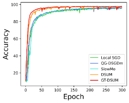
(a) non-IID $=0.1$

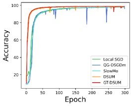
(b) non-IID $=1$

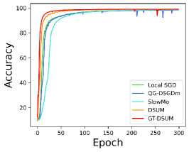
(c) non-IID $=10$

Figure 4: Testing accuracy for various tasks training on LeNet over MNIST.

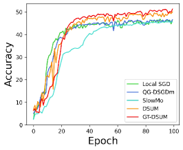
(a) non-IID $=0.1$

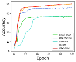
(b) non-IID $=1$

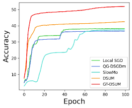
(c) non-IID $=10$

Figure 5: Testing accuracy for various tasks training on CNN over EMNIST.

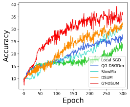
(a) non-IID $=0.1$

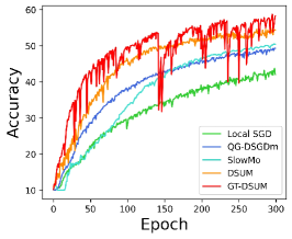
(b) non-IID $=1$

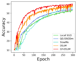
(c) non-IID $=10$

Figure 6: Testing accuracy for various tasks training on LeNet over CIFAR10.

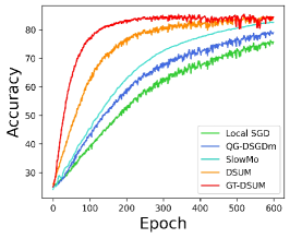
(a) non-IID $=0.1$

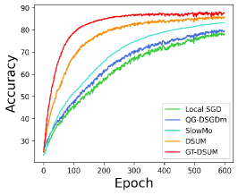
(b) non-IID $=1$

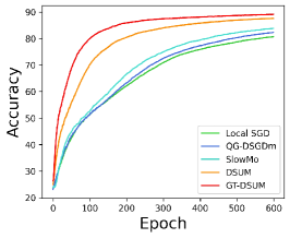
(c) non-IID $=10$

Figure 7: Testing accuracy for various tasks training on RNN over AG NEWS.

References

• Cohen et al. [2017] Gregory Cohen, Saeed Afshar, Jonathan Tapson, and Andre Van Schaik. EMNIST: Extending mnist to handwritten letters. 2017 international joint conference on neural networks (IJCNN), pages 2921–2926, 2017.
• Cutkosky and Mehta [2020] Ashok Cutkosky and Harsh Mehta. Momentum improves normalized SGD. International Conference on Machine Learning, pages 2260–2268, 2020.
• Deng and Gao [2021] Qi Deng and Wenzhi Gao. Minibatch and momentum model-based methods for stochastic weakly convex optimization. Advances in Neural Information Processing Systems, 34, 2021.
• Di Lorenzo and Scutari [2016] Paolo Di Lorenzo and Gesualdo Scutari. Next: In-network nonconvex optimization. IEEE Transactions on Signal and Information Processing over Networks, 2(2):120–136, 2016.
• Esfandiari et al. [2021] Yasaman Esfandiari, Sin Yong Tan, Zhanhong Jiang, Aditya Balu, Ethan Herron, Chinmay Hegde, and Soumik Sarkar. Cross-gradient aggregation for decentralized learning from non-IID data. International Conference on Machine Learning, pages 3036–3046, 2021.
• Fang et al. [2018] Cong Fang, Chris Junchi Li, Zhouchen Lin, and Tong Zhang. Spider: Near-optimal non-convex optimization via stochastic path-integrated differential estimator. Advances in Neural Information Processing Systems, 31, 2018.
• Ghadimi et al. [2015] Euhanna Ghadimi, Hamid Reza Feyzmahdavian, and Mikael Johansson. Global convergence of the heavy-ball method for convex optimization. 2015 European control conference (ECC), pages 310–315, 2015.
• Han and Gao [2021] Andi Han and Junbin Gao. Riemannian stochastic recursive momentum method for non-convex optimization. International Joint Conference on Artificial Intelligence, 2021.
• Hsieh et al. [2020] Kevin Hsieh, Amar Phanishayee, Onur Mutlu, and Phillip Gibbons. The non-IID data quagmire of decentralized machine learning. International Conference on Machine Learning, pages 4387–4398, 2020.
• Karimireddy et al. [2020] Sai Praneeth Karimireddy, Satyen Kale, Mehryar Mohri, Sashank Reddi, Sebastian Stich, and Ananda Theertha Suresh. SCAFFOLD: Stochastic controlled averaging for federated learning. International Conference on Machine Learning, pages 5132–5143, 2020.
• Kingma and Ba [2015] Diederik P. Kingma and Jimmy Ba. Adam: A method for stochastic optimization. 2015.
• Koloskova et al. [2019] Anastasia Koloskova, Sebastian Stich, and Martin Jaggi. Decentralized stochastic optimization and gossip algorithms with compressed communication. International Conference on Machine Learning, pages 3478–3487, 2019.
• Koloskova et al. [2020] Anastasia Koloskova, Nicolas Loizou, Sadra Boreiri, Martin Jaggi, and Sebastian Stich. A unified theory of decentralized SGD with changing topology and local updates. International Conference on Machine Learning, pages 5381–5393, 2020.
• Koloskova et al. [2021] Anastasiia Koloskova, Tao Lin, and Sebastian U Stich. An improved analysis of gradient tracking for decentralized machine learning. Advances in Neural Information Processing Systems, 34, 2021.
• Krizhevsky et al. [2009] Alex Krizhevsky, Geoffrey Hinton, et al. Learning multiple layers of features from tiny images. 2009.
• LeCun et al. [1998] Yann LeCun, Léon Bottou, Yoshua Bengio, and Patrick Haffner. Gradient-based learning applied to document recognition. Proceedings of the IEEE, 86(11):2278–2324, 1998.
• Lian et al. [2017] Xiangru Lian, Ce Zhang, Huan Zhang, Cho-Jui Hsieh, Wei Zhang, and Ji Liu. Can decentralized algorithms outperform centralized algorithms? A case study for decentralized parallel stochastic gradient descent. Advances in Neural Information Processing Systems, 30, 2017.
• Lin et al. [2021] Tao Lin, Sai Praneeth Karimireddy, Sebastian U Stich, and Martin Jaggi. Quasi-global momentum: accelerating decentralized deep learning on heterogeneous data. International Conference on Machine Learning, pages 6654–6665, 2021.
• Mai and Johansson [2020] Vien Mai and Mikael Johansson. Convergence of a stochastic gradient method with momentum for non-smooth non-convex optimization. International Conference on Machine Learning, pages 6630–6639, 2020.
• Moritz et al. [2018] Philipp Moritz, Robert Nishihara, Stephanie Wang, Alexey Tumanov, Richard Liaw, Eric Liang, Melih Elibol, Zongheng Yang, William Paul, Michael I. Jordan, and Ion Stoica. Ray: A distributed framework for emerging ai applications. Proceedings of the 13th USENIX Conference on Operating Systems Design and Implementation, page 561–577, 2018.
• Nesterov [1983] Yurii E Nesterov. A method for solving the convex programming problem with convergence rate $o(1/k^{2})$. Dokl. akad. nauk Sssr, 269:543–547, 1983.
• Polyak [1964] Boris T Polyak. Some methods of speeding up the convergence of iteration methods. Ussr computational mathematics and mathematical physics, 4(5):1–17, 1964.
• Qu et al. [2022] Zhe Qu, Xingyu Li, LuZhuo Duan, Rui, Yao Liu, and Bo Tang. Generalized federated learning via sharpness aware minimization. International Conference on Machine Learning, 2022.
• Reddi et al. [2020] Sashank J Reddi, Zachary Charles, Manzil Zaheer, Zachary Garrett, Keith Rush, Jakub Konečnỳ, Sanjiv Kumar, and Hugh Brendan McMahan. Adaptive federated optimization. International Conference on Learning Representations, 2020.
• Shang et al. [2022] Xinyi Shang, Yang Lu, Gang Huang, and Hanzi Wang. Federated learning on heterogeneous and long-tailed data via classifier re-training with federated features. International Joint Conference on Artificial Intelligence, pages 2218–2224, 2022.
• Stich [2018] Sebastian U Stich. Local SGD converges fast and communicates little. International Conference on Learning Representations, 2018.
• Tao et al. [2021] Wei Tao, Sheng Long, Gaowei Wu, and Qing Tao. The role of momentum parameters in the optimal convergence of adaptive Polyak’s Heavy-ball methods. 9th International Conference on Learning Representations, ICLR, 2021.
• Tao et al. [2022] Youming Tao, Yulian Wu, Xiuzhen Cheng, and Di Wang. Private stochastic convex optimization and sparse learning with heavy-tailed data revisited. International Joint Conference on Artificial Intelligence, 2022.
• Wan et al. [2022] Wei Wan, Shengshan Hu, Jianrong Lu, Leo Yu Zhang, Hai Jin, and Yuanyuan He. Shielding federated learning: Robust aggregation with adaptive client selection. International Joint Conference on Artificial Intelligence, 2022.
• Wang et al. [2020] Jianyu Wang, Vinayak Tantia, Nicolas Ballas, and Michael G. Rabbat. Slowmo: Improving communication-efficient distributed SGD with slow momentum. 8th International Conference on Learning Representations, ICLR, 2020.
• Xin et al. [2021a] Ran Xin, Usman Khan, and Soummya Kar. A hybrid variance-reduced method for decentralized stochastic non-convex optimization. International Conference on Machine Learning, pages 11459–11469, 2021.
• Xin et al. [2021b] Ran Xin, Usman A Khan, and Soummya Kar. An improved convergence analysis for decentralized online stochastic non-convex optimization. IEEE Transactions on Signal Processing, 69:1842–1858, 2021.
• Xu et al. [2021] Hang Xu, Chen-Yu Ho, Ahmed M. Abdelmoniem, Aritra Dutta, EH Bergou, Konstantinos Karatsenidis, Marco Canini, and Panos Kalnis. GRACE: A compressed communication framework for distributed machine learning. In Proc. of 41st IEEE Int. Conf. Distributed Computing Systems (ICDCS), 2021.
• Yan et al. [2018] Yan Yan, Tianbao Yang, Zhe Li, Qihang Lin, and Yi Yang. A unified analysis of stochastic momentum methods for deep learning. Proceedings of the 27th International Joint Conference on Artificial Intelligence, pages 2955–2961, 2018.
• Yu et al. [2019] Hao Yu, Rong Jin, and Sen Yang. On the linear speedup analysis of communication efficient momentum SGD for distributed non-convex optimization. International Conference on Machine Learning, pages 7184–7193, 2019.
• Zhang et al. [2015] Xiang Zhang, Junbo Zhao, and Yann LeCun. Character-level convolutional networks for text classification. Advances in neural information processing systems, 28, 2015.
• Zhang et al. [2022] Hong Zhang, Ji Liu, Juncheng Jia, Yang Zhou, Huaiyu Dai, and Dejing Dou. FedDUAP: Federated learning with dynamic update and adaptive pruning using shared data on the server. International Joint Conference on Artificial Intelligence, 2022.